asphalt materials characterization in … · final contract report asphalt materials...

ASPHALT MATERIALS CHARACTERIZATION

IN SUPPORT OF IMPLEMENTATION

OF THE PROPOSED MECHANISTIC-EMPIRICAL

PAVEMENT DESIGN GUIDE

FINALCONTRACT REPORT

VTRC 07-CR10

http://www.virginiadot.org/vtrc/main/online_reports/pdf/07-cr10.pdf

GERARDO W. FLINTSCH, Ph.D., P.E.Director, Center for Sustainable Transportation Infrastructure

VTTI, Virginia Tech

AMARA LOULIZI, Ph.D., P.E.Research Scientist, CSTI

VTTI, Virginia Tech

STACEY D. DIEFENDERFERResearch Scientist

Virginia Transportation Research Council

KHALED A. GALAL, Ph.D.Research Scientist


BRIAN K. DIEFENDERFER, Ph.D.Research Scientist


http://www.virginiadot.org/vtrc/main/online_reports/pdf/07-cr10.pdf

borrego

Typewritten Text

Copyright by the Virginia Center for Transportation Innovation and Research. Gerardo W. Flintsch, Amara Loulizi, Stacey D. Diefenderfer, Khaled A. Galal, and Brian K. Diefenderfer. “Asphalt Materials Characterization in Support of Implementation of the Proposed Mechanistic-Empirical Pavement Design Guide,” Virginia Transportation Research Council 530 Edgemont Road Charlottesville, VA 22903, Report No. VTRC 07-CR10, Jan. 2007.

borrego

Typewritten Text

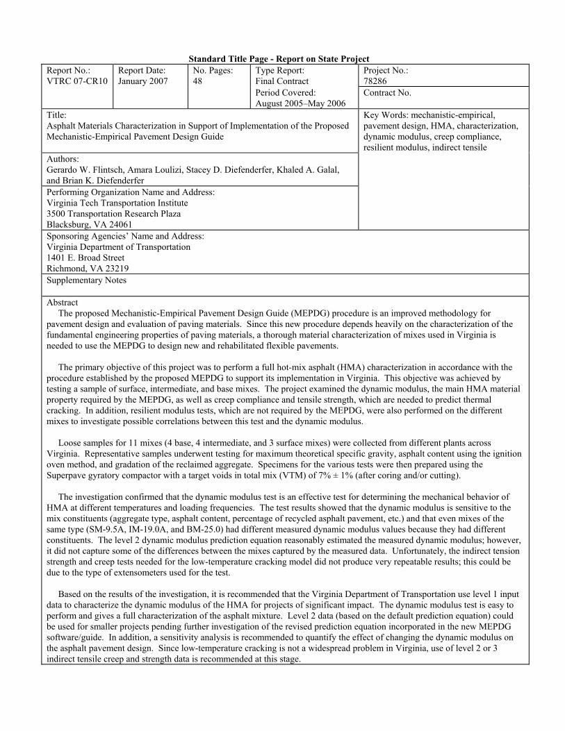
Standard Title Page - Report on State Project Report No.: VTRC 07-CR10

Report Date: January 2007

No. Pages: 48

Type Report: Final Contract

Project No.: 78286

Period Covered: August 2005–May 2006

Contract No.

Title: Asphalt Materials Characterization in Support of Implementation of the Proposed Mechanistic-Empirical Pavement Design Guide

Key Words: mechanistic-empirical, pavement design, HMA, characterization, dynamic modulus, creep compliance, resilient modulus, indirect tensile

Authors: Gerardo W. Flintsch, Amara Loulizi, Stacey D. Diefenderfer, Khaled A. Galal, and Brian K. Diefenderfer

Performing Organization Name and Address: Virginia Tech Transportation Institute 3500 Transportation Research Plaza Blacksburg, VA 24061

Sponsoring Agencies’ Name and Address: Virginia Department of Transportation 1401 E. Broad Street Richmond, VA 23219 Supplementary Notes Abstract The proposed Mechanistic-Empirical Pavement Design Guide (MEPDG) procedure is an improved methodology for pavement design and evaluation of paving materials. Since this new procedure depends heavily on the characterization of the fundamental engineering properties of paving materials, a thorough material characterization of mixes used in Virginia is needed to use the MEPDG to design new and rehabilitated flexible pavements. The primary objective of this project was to perform a full hot-mix asphalt (HMA) characterization in accordance with the procedure established by the proposed MEPDG to support its implementation in Virginia. This objective was achieved by testing a sample of surface, intermediate, and base mixes. The project examined the dynamic modulus, the main HMA material property required by the MEPDG, as well as creep compliance and tensile strength, which are needed to predict thermal cracking. In addition, resilient modulus tests, which are not required by the MEPDG, were also performed on the different mixes to investigate possible correlations between this test and the dynamic modulus. Loose samples for 11 mixes (4 base, 4 intermediate, and 3 surface mixes) were collected from different plants across Virginia. Representative samples underwent testing for maximum theoretical specific gravity, asphalt content using the ignition oven method, and gradation of the reclaimed aggregate. Specimens for the various tests were then prepared using the Superpave gyratory compactor with a target voids in total mix (VTM) of 7% ± 1% (after coring and/or cutting). The investigation confirmed that the dynamic modulus test is an effective test for determining the mechanical behavior of HMA at different temperatures and loading frequencies. The test results showed that the dynamic modulus is sensitive to the mix constituents (aggregate type, asphalt content, percentage of recycled asphalt pavement, etc.) and that even mixes of the same type (SM-9.5A, IM-19.0A, and BM-25.0) had different measured dynamic modulus values because they had different constituents. The level 2 dynamic modulus prediction equation reasonably estimated the measured dynamic modulus; however, it did not capture some of the differences between the mixes captured by the measured data. Unfortunately, the indirect tension strength and creep tests needed for the low-temperature cracking model did not produce very repeatable results; this could be due to the type of extensometers used for the test. Based on the results of the investigation, it is recommended that the Virginia Department of Transportation use level 1 input data to characterize the dynamic modulus of the HMA for projects of significant impact. The dynamic modulus test is easy to perform and gives a full characterization of the asphalt mixture. Level 2 data (based on the default prediction equation) could be used for smaller projects pending further investigation of the revised prediction equation incorporated in the new MEPDG software/guide. In addition, a sensitivity analysis is recommended to quantify the effect of changing the dynamic modulus on the asphalt pavement design. Since low-temperature cracking is not a widespread problem in Virginia, use of level 2 or 3 indirect tensile creep and strength data is recommended at this stage.

FINAL CONTRACT REPORT

ASPHALT MATERIALS CHARACTERIZATION IN SUPPORT OF IMPLEMENTATION OF THE PROPOSED MECHANISTIC-EMPIRICAL


Gerardo W. Flintsch, Ph.D., P.E. Director, Center for Sustainable Transportation Infrastructure, VTTI, Virginia Tech

Amara Loulizi, Ph.D., P.E.

Research Scientist, CSTI, VTTI, Virginia Tech

Stacey D. Diefenderfer Research Scientist, Virginia Transportation Research Council

Khaled A. Galal, Ph.D.

Research Scientist, Virginia Transportation Research Council

Brian K. Diefenderfer, Ph.D. Research Scientist, Virginia Transportation Research Council

Project Manager Stacey D. Diefenderfer, Virginia Transportation Research Council

Contract Research Sponsored by the Virginia Transportation Research Council

Virginia Transportation Research Council (A partnership of the Virginia Department of Transportation

and the University of Virginia since 1948)

Charlottesville, Virginia

January 2007 VTRC 07-CR10

ii

NOTICE

The project that is the subject of this report was done under contract for the Virginia Department of Transportation, Virginia Transportation Research Council. The contents of this report reflect the views of the authors, who are responsible for the facts and the accuracy of the data presented herein. The contents do not necessarily reflect the official views or policies of the Virginia Department of Transportation, the Commonwealth Transportation Board, or the Federal Highway Administration. This report does not constitute a standard, specification, or regulation. Each contract report is peer reviewed and accepted for publication by Research Council staff with expertise in related technical areas. Final editing and proofreading of the report are performed by the contractor.

Copyright 2007 by the Commonwealth of Virginia. All rights reserved.

iii

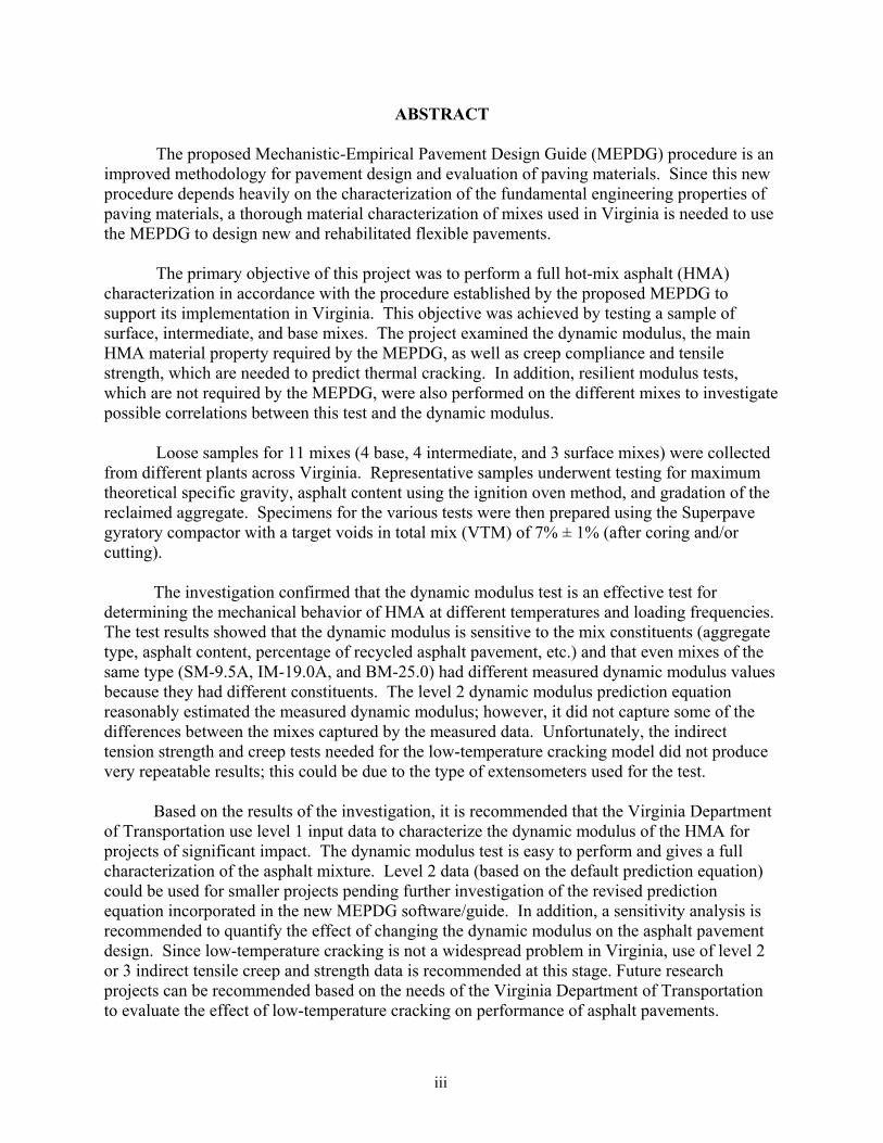
ABSTRACT

The proposed Mechanistic-Empirical Pavement Design Guide (MEPDG) procedure is an improved methodology for pavement design and evaluation of paving materials. Since this new procedure depends heavily on the characterization of the fundamental engineering properties of paving materials, a thorough material characterization of mixes used in Virginia is needed to use the MEPDG to design new and rehabilitated flexible pavements.

The primary objective of this project was to perform a full hot-mix asphalt (HMA)

characterization in accordance with the procedure established by the proposed MEPDG to support its implementation in Virginia. This objective was achieved by testing a sample of surface, intermediate, and base mixes. The project examined the dynamic modulus, the main HMA material property required by the MEPDG, as well as creep compliance and tensile strength, which are needed to predict thermal cracking. In addition, resilient modulus tests, which are not required by the MEPDG, were also performed on the different mixes to investigate possible correlations between this test and the dynamic modulus.

Loose samples for 11 mixes (4 base, 4 intermediate, and 3 surface mixes) were collected

from different plants across Virginia. Representative samples underwent testing for maximum theoretical specific gravity, asphalt content using the ignition oven method, and gradation of the reclaimed aggregate. Specimens for the various tests were then prepared using the Superpave gyratory compactor with a target voids in total mix (VTM) of 7% ± 1% (after coring and/or cutting).

The investigation confirmed that the dynamic modulus test is an effective test for determining the mechanical behavior of HMA at different temperatures and loading frequencies. The test results showed that the dynamic modulus is sensitive to the mix constituents (aggregate type, asphalt content, percentage of recycled asphalt pavement, etc.) and that even mixes of the same type (SM-9.5A, IM-19.0A, and BM-25.0) had different measured dynamic modulus values because they had different constituents. The level 2 dynamic modulus prediction equation reasonably estimated the measured dynamic modulus; however, it did not capture some of the differences between the mixes captured by the measured data. Unfortunately, the indirect tension strength and creep tests needed for the low-temperature cracking model did not produce very repeatable results; this could be due to the type of extensometers used for the test.

Based on the results of the investigation, it is recommended that the Virginia Department

of Transportation use level 1 input data to characterize the dynamic modulus of the HMA for projects of significant impact. The dynamic modulus test is easy to perform and gives a full characterization of the asphalt mixture. Level 2 data (based on the default prediction equation) could be used for smaller projects pending further investigation of the revised prediction equation incorporated in the new MEPDG software/guide. In addition, a sensitivity analysis is recommended to quantify the effect of changing the dynamic modulus on the asphalt pavement design. Since low-temperature cracking is not a widespread problem in Virginia, use of level 2 or 3 indirect tensile creep and strength data is recommended at this stage. Future research projects can be recommended based on the needs of the Virginia Department of Transportation to evaluate the effect of low-temperature cracking on performance of asphalt pavements.

FINAL CONTRACT REPORT

ASPHALT MATERIALS CHARACTERIZATION IN SUPPORT OF IMPLEMENTATION OF THE PROPOSED MECHANISTIC-EMPIRICAL


Gerardo W. Flintsch, Ph.D., P.E. Director, Center for Sustainable Transportation Infrastructure, VTTI, Virginia Tech

Amara Loulizi, Ph.D., P.E.

Research Scientist, CSTI, VTTI, Virginia Tech

Stacey D. Diefenderfer Research Scientist, Virginia Transportation Research Council

Khaled A. Galal, Ph.D.

Research Scientist, Virginia Transportation Research Council

Brian K. Diefenderfer, Ph.D. Research Scientist, Virginia Transportation Research Council

INTRODUCTION

The proposed Mechanistic-Empirical Pavement Design Guide (MEPDG) procedure, introduced in NCHRP Project 1-37A (NCHRP, 2004), is an improved methodology for pavement design and evaluation of paving materials. Unlike currently used empirical pavement design methods, this new procedure depends heavily on the characterization of the fundamental engineering properties of paving materials. For asphaltic materials, the term material characterization can be defined as the measurements and the analysis of the asphaltic material response to load and deformation at different loading rates or temperatures (i.e., environmental conditions). Implementation of the MEPDG in Virginia is expected to improve the efficiency of pavement designs, provide better capability for prediction of pavement lifetime maintenance needs, and strengthen Virginia’s position as a leading state in emerging technology.

Use of the proposed MEPDG for the design of asphalt pavements requires a

comprehensive characterization of the materials typically used in Virginia pavements. The MEPDG identifies and incorporates several fundamental properties and tests for asphalt mixtures and binders. The data required for asphalt mixtures include indirect tensile strength, creep compliance, and dynamic modulus. The required asphalt binder properties include the complex shear modulus and associated phase angle. General asphalt mixture properties include asphalt binder content, aggregate gradation, and volumetric properties. These material characteristics are also necessary to calibrate the proposed MEPDG for use with materials used in Virginia pavements. Accurate knowledge of these characteristics and calibration of the design guide will improve the efficiency and reliability of future asphalt pavement designs for new construction and rehabilitation in Virginia.

2

PURPOSE AND SCOPE

A thorough material characterization of hot-mix asphalt (HMA) mixes used in Virginia is needed to use the proposed MEPDG to design new and rehabilitated flexible pavements. These tests would provide level 1 input for the HMA material properties as required for the highest-priority flexible pavement designs. In addition, even for the level 2 input, the equations relating volumetric properties to the required mechanical properties need to be validated and possibly calibrated for the mixes used in Virginia. Level 3 designs require catalogued properties of the typical mixes used in Virginia, which are set as default values for the pavement designer.

Therefore, the primary objective of this project was to perform a full HMA material

characterization in accordance with the procedure established by the proposed MEPDG in order to support the implementation of mechanistic-empirical pavement design procedures in Virginia. This objective was achieved by testing a sample of HMA used in Virginia as surface, intermediate, and base mixes. Dynamic modulus and creep compliance temperatures were measured at the recommended temperatures and frequencies for 11 typical mixes.

In addition, resilient modulus tests, which are not required by the MEPDG, were also

performed on the different mixes in order to investigate possible correlations between this test and the dynamic modulus. The resilient modulus is used with the AASHTO 1993 pavement design method currently used in VDOT and for pavement analysis using multilayer linear elastic analysis software (e.g., ELSYM5) to calculate stresses and strains in the pavement.

METHODS AND MATERIALS

The main HMA material property required by the MEPDG is the dynamic modulus. Additional properties, namely the creep compliance and the tensile strength, are needed to predict thermal cracking. The dynamic modulus test was performed in accordance with AASHTO TP62-03. Five testing temperatures were used: 10°F, 30°F, 70°F, 100°F, and 130°F. Six testing frequencies, 0.1 Hz, 0.5 Hz, 1 Hz, 5 Hz, 10 Hz, and 25 Hz, were used at each temperature. Three specimens per mix were tested. Each specimen was first tested at the lowest temperature with all six frequencies from highest to lowest. The procedure was then repeated at consecutively higher temperatures until the sequence had been completed for all specimens. The creep test was performed in accordance with AASHTO T322-03. The three standard testing temperatures were used: −4°F, 14°F, and 32°F. At each temperature, a static load was applied for 100 seconds. Two specimens per mix were tested. The same specimens were then used to determine the mix tensile strength at 14°F. The resilient modulus test was performed in accordance with ASTM D4123 at the following three testing temperatures: 41°F, 77°F, and 104°F. Two specimens per mix were tested.

This study used 11 mixes. In total, 33 specimens were tested for dynamic modulus, 22

for creep compliance and tensile strength, and 22 for resilient modulus. The following section describes the 11 mixes and discusses the procedures used for preparing the specimens.

3

Specimen Preparation and Volumetric Analysis Loose samples for 11 mixes were collected from different plants across the

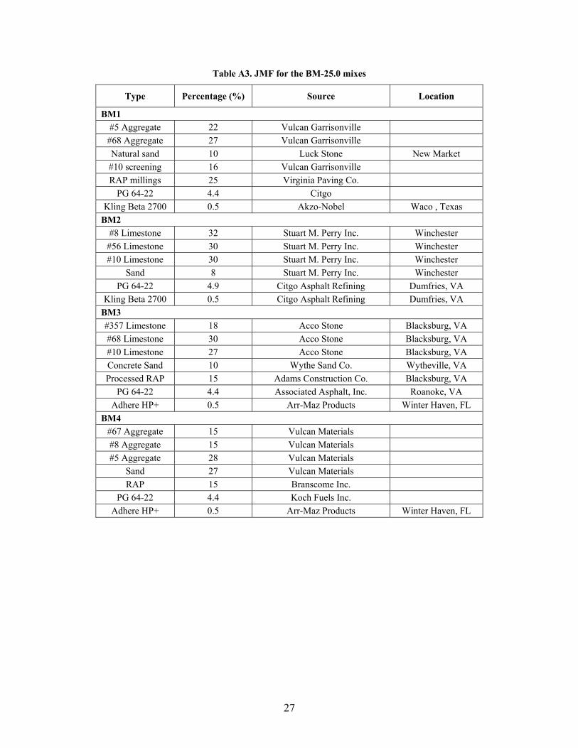
Commonwealth of Virginia. The mixes consisted of 4 base mixes (BM-25.0), 4 intermediate mixes (IM-19.0A), and 3 surface mixes (SM-9.5A). The mixes were labeled depending on their mix type (BM, IM, and SM) and were numbered randomly. The labels for the different mixes and the plants where they were collected are presented in Table 1. The job-mix formulas (JMF) for all the mixes are presented in Tables A1 to A3 in Appendix A.

Table 1. Labels and plant locations of mixes

Mix Type Label Contractor Location SM1 VA Paving Corp. Stafford SM2 ADAMS Rockydale SM-9.5A SM3 Superior Paving Warrenton IM1 APAC Occoquan IM2 Branscome Norfolk IM3 Adams Lowmoor IM-19.0A

IM4 B&S Contracting Augusta BM1 VA Paving Corp. Stafford BM2 Stuart M. Perry Winchester BM3 Adams Blacksburg BM-25.0

BM4 Branscome Norfolk Once the mixes were collected, representative samples were used to perform the

following tests: maximum theoretical specific gravity (Gmm) in accordance with AASHTO T209, asphalt content using the ignition method, and gradation of the reclaimed aggregate in accordance with AASHTO T27. Each of these tests was performed on four samples. Results of the individual tests are presented in Tables B1 to B11 in Appendix B. Table 2, Table 3, and Table 4 show the average properties for the SM-9.5A, IM-19.0A, and BM-25.0 mixes, respectively. The values that did not pass the acceptance range are shaded in gray. Although some properties were outside of the acceptance range, no mixture failed to the extent that they were removed and replaced.

Table 2. Asphalt content, Gmm, and aggregate gradation for the SM-9.5A mixes

SM1 SM2 SM3 Avg. JMF Avg. JMF Avg. JMF

Asp. Ct. (%) 4.93 5.3 ± 0.3 5.91 5.9 ± 0.3 6.32 5.6 ± 0.3 Gmm 2.630 2.626 2.648 2.618 2.596 2.599

Gradation Sieve opening, mm

(No.) %

Passing Acceptance

Range %

Passing Acceptance

Range %

Passing Acceptance

Range 12.5 (1/2) 97.4 100 100.0 99-100 99.2 99-100 9.5 (3/8) 89.9 89-97 96.3 92-100 91.4 89-97 4.75 (#4) 57.2 56-64 57.1 56-64 55.8 55-63 2.36 (#8) 37.9 36-44 37.6 37-45 39.5 36-44

1.18 (#16) 27.9 - 28.1 - 30.0 - 0.6 (#30) 19.4 - 20.2 - 21.5 - 0.3 (#50) 10.9 - 12.8 - 13.4 -

0.15 (#100) 6.8 - 8.5 - 9.1 - 0.075 (#200) 5.0 4-6 6.3 4.9-6.9 6.3 4.7-6.7

4

Table 3. Asphalt content, Gmm, and aggregate gradation for the IM-19.0A mixes IM1 IM2 IM3 IM4 Avg. JMF Avg. JMF Avg. JMF Avg. JMF

Asphalt content (%) 5.26 4.6 ± 0.3 4.52 4.6 ± 0.3 4.89 4.9 ± 0.3 5.43 5.5 ± 0.3

Gmm 2.477 2.504 2.513 2.500 2.523 2.524 2.486 2.502 Gradation

Sieve opening, mm (No.)

% Passing

Accept. Range

% Passing

Accept. Range

% Passing

Accept. Range

% Passing

Accept. Range

25 (1) 100.0 100 100.0 100 100.0 100 100.0 100 19 (3/4) 100.0 92-100 97.6 92-100 96.4 92-100 98.8 92-100

12.5 (1/2) 95.8 84-92 84.6 80-88 79.8 76-84 85.3 82-90 9.5 (3/8) 87.5 - 73.3 - 69.5 - 75.4 - 4.75 (#4) 53.0 - 41.5 - 45.6 - 58.5 - 2.36 (#8) 37.7 29-37 29.8 29-37 30.4 28-36 40.0 26-34 1.18 (#16) 29.4 - 24.2 - 21.1 - 30.3 - 0.6 (#30) 21.8 - 18.1 - 15.4 - 23.4 - 0.3 (#50) 14.5 - 11.5 - 10.4 - 14.4 -

0.15 (#100) 9.9 - 6.6 - 7.2 - 8.0 - 0.075 (#200) 6.6 4-6 3.8 3.4-5.4 5.5 4-6 5.9 4-6

Table 4. Asphalt content, Gmm, and aggregate gradation for BM-25.0 mixes

BM1 BM2 BM3 BM4 Avg. JMF Avg. JMF Avg. JMF Avg. JMF

Asphalt content (%) 4.62 4.4 ± 0.3 4.86 4.9 ± 0.3 3.91 4.4 ± 0.3 4.51 4.4 ± 0.3

Gmm 2.691 2.668 2.509 2.515 2.640 2.605 2.516 2.525 Gradation


% Passing

Accept. Range

% Passing

Accept. Range

% Passing

Accept. Range

% Passing

Accept. Range

37.5 (1.5) 100.0 100 100.0 100 100.0 100 100.0 100 25 (1) 99.2 92-100 84.1 90-98 97.3 90-98 100.0 92-100

19 (3/4) 94.4 82-90 73.8 73-81 87.6 82-90 95.5 81-89 12.5 (1/2) 75.9 - 69.6 - 73.3 - 82.5 - 9.5 (3/8) 66.0 - 66.6 - 64.8 - 70.6 - 4.75 (#4) 46.3 - 42.9 - 48.0 - 41.1 - 2.36 (#8) 31.3 26-34 26.5 25-33 24.2 25-33 30.3 33-41 1.18 (#16) 23.0 - 17.0 - 17.1 - 24.7 - 0.6 (#30) 16.6 - 11.4 - 13.1 - 18.2 - 0.3 (#50) 10.6 - 8.2 - 8.9 - 11.0 -

0.15 (#100) 7.4 - 6.5 - 7.1 - 6.2 - 0.075 (#200) 5.4 3-5 5.5 3.6-5.6 6.1 4-6 3.9 3.2-5.2

5

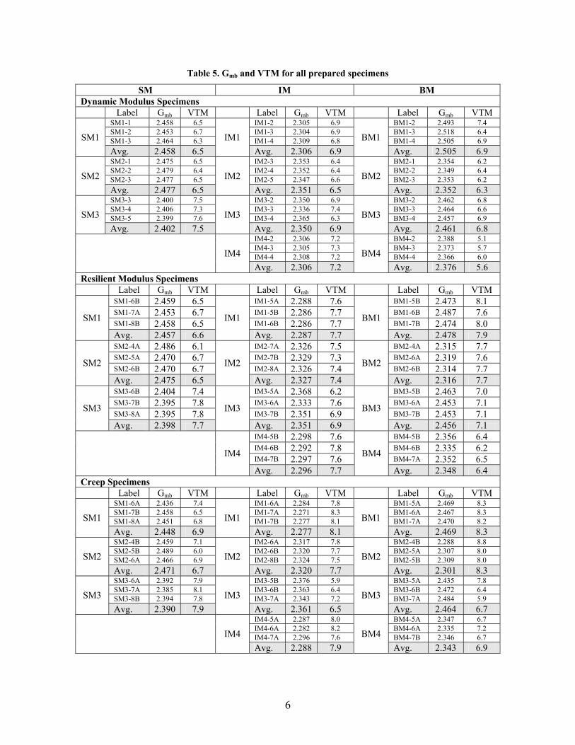
Once the Gmm, asphalt content, and aggregate gradation of the mixes were determined, the Superpave gyratory compactor was used to prepare the specimens for testing. A target voids in total mix (VTM) of 7% ± 1% was intended for all the specimens (after coring and/or cutting), which is approximately the air void content of newly constructed pavements in Virginia. Several trial specimens per mix were prepared before achieving the correct mix weight. The prepared gyratory specimen was 6 inches in diameter by 7 inches in height, thus, the number of gyrations was left variable to achieve the specified height of 7 inches. The prepared gyratory specimen was cut to 6 inches in thickness and cored to 4 inches in diameter to get the specimen for dynamic modulus testing.

For the resilient modulus and creep specimens, the ends (top and bottom 0.5 inch) of the

gyratory specimen were removed, and then the top and bottom 1.5 inches were cut to obtain two specimens. The final dimensions of the specimens were 6 inches in diameter and 1.5 inches in thickness. Figure 1 shows a typical specimen for dynamic modulus and for the resilient modulus or creep tests. The bulk specific gravity (Gmb) of all produced specimens was measured using the AASHTO T166 procedure. Table 5 presents the measured Gmb and calculated VTM for all specimens prepared for the dynamic modulus, resilient modulus, and creep tests. The table shows that most prepared specimens met the VTM requirements of 7% ± 1% except for the dynamic modulus specimens for BM4. For this mix, decreasing the weight of mix placed in the gyratory to produce higher voids resulted in samples that broke after extraction from the gyratory machine. The first sample that held together provided a dynamic modulus specimen with a VTM of 5.1% as shown in Table 5. In addition, a few specimens had a VTM slightly above 8.0%.

Figure 1. Typical specimens for (a) dynamic modulus and (b) resilient modulus and creep test

(a) (b)

6

Table 5. Gmb and VTM for all prepared specimens

SM IM BM Dynamic Modulus Specimens

Label Gmb VTM Label Gmb VTM Label Gmb VTM SM1-1 2.458 6.5 IM1-2 2.305 6.9 BM1-2 2.493 7.4 SM1-2 2.453 6.7 IM1-3 2.304 6.9 BM1-3 2.518 6.4 SM1-3 2.464 6.3 IM1-4 2.309 6.8 BM1-4 2.505 6.9 SM1 Avg. 2.458 6.5

IM1 Avg. 2.306 6.9

BM1 Avg. 2.505 6.9

SM2-1 2.475 6.5 IM2-3 2.353 6.4 BM2-1 2.354 6.2 SM2-2 2.479 6.4 IM2-4 2.352 6.4 BM2-2 2.349 6.4 SM2-3 2.477 6.5 IM2-5 2.347 6.6 BM2-3 2.353 6.2 SM2 Avg. 2.477 6.5

IM2 Avg. 2.351 6.5

BM2 Avg. 2.352 6.3

SM3-3 2.400 7.5 IM3-2 2.350 6.9 BM3-2 2.462 6.8 SM3-4 2.406 7.3 IM3-3 2.336 7.4 BM3-3 2.464 6.6 SM3-5 2.399 7.6 IM3-4 2.365 6.3 BM3-4 2.457 6.9 SM3 Avg. 2.402 7.5

IM3 Avg. 2.350 6.9

BM3 Avg. 2.461 6.8

IM4-2 2.306 7.2 BM4-2 2.388 5.1 IM4-3 2.305 7.3 BM4-3 2.373 5.7 IM4-4 2.308 7.2 BM4-4 2.366 6.0 IM4 Avg. 2.306 7.2

BM4 Avg. 2.376 5.6

Resilient Modulus Specimens Label Gmb VTM Label Gmb VTM Label Gmb VTM

SM1-6B 2.459 6.5 IM1-5A 2.288 7.6 BM1-5B 2.473 8.1 SM1-7A 2.453 6.7 IM1-5B 2.286 7.7 BM1-6B 2.487 7.6 SM1-8B 2.458 6.5 IM1-6B 2.286 7.7 BM1-7B 2.474 8.0 SM1

Avg. 2.457 6.6

IM1

Avg. 2.287 7.7

BM1

Avg. 2.478 7.9 SM2-4A 2.486 6.1 IM2-7A 2.326 7.5 BM2-4A 2.315 7.7 SM2-5A 2.470 6.7 IM2-7B 2.329 7.3 BM2-6A 2.319 7.6 SM2-6B 2.470 6.7 IM2-8A 2.326 7.4 BM2-6B 2.314 7.7 SM2

Avg. 2.475 6.5

IM2

Avg. 2.327 7.4

BM2

Avg. 2.316 7.7 SM3-6B 2.404 7.4 IM3-5A 2.368 6.2 BM3-5B 2.463 7.0 SM3-7B 2.395 7.8 IM3-6A 2.333 7.6 BM3-6A 2.453 7.1 SM3-8A 2.395 7.8 IM3-7B 2.351 6.9 BM3-7B 2.453 7.1 SM3

Avg. 2.398 7.7

IM3

Avg. 2.351 6.9

BM3

Avg. 2.456 7.1 IM4-5B 2.298 7.6 BM4-5B 2.356 6.4 IM4-6B 2.292 7.8 BM4-6B 2.335 6.2 IM4-7B 2.297 7.6 BM4-7A 2.352 6.5 IM4

Avg. 2.296 7.7

BM4

Avg. 2.348 6.4 Creep Specimens

Label Gmb VTM Label Gmb VTM Label Gmb VTM SM1-6A 2.436 7.4 IM1-6A 2.284 7.8 BM1-5A 2.469 8.3 SM1-7B 2.458 6.5 IM1-7A 2.271 8.3 BM1-6A 2.467 8.3 SM1-8A 2.451 6.8 IM1-7B 2.277 8.1 BM1-7A 2.470 8.2 SM1 Avg. 2.448 6.9

IM1 Avg. 2.277 8.1

BM1 Avg. 2.469 8.3

SM2-4B 2.459 7.1 IM2-6A 2.317 7.8 BM2-4B 2.288 8.8 SM2-5B 2.489 6.0 IM2-6B 2.320 7.7 BM2-5A 2.307 8.0 SM2-6A 2.466 6.9 IM2-8B 2.324 7.5 BM2-5B 2.309 8.0 SM2 Avg. 2.471 6.7

IM2 Avg. 2.320 7.7

BM2 Avg. 2.301 8.3

SM3-6A 2.392 7.9 IM3-5B 2.376 5.9 BM3-5A 2.435 7.8 SM3-7A 2.385 8.1 IM3-6B 2.363 6.4 BM3-6B 2.472 6.4 SM3-8B 2.394 7.8 IM3-7A 2.343 7.2 BM3-7A 2.484 5.9 SM3 Avg. 2.390 7.9

IM3 Avg. 2.361 6.5

BM3 Avg. 2.464 6.7

IM4-5A 2.287 8.0 BM4-5A 2.347 6.7 IM4-6A 2.282 8.2 BM4-6A 2.335 7.2 IM4-7A 2.296 7.6 BM4-7B 2.346 6.7 IM4 Avg. 2.288 7.9

BM4 Avg. 2.343 6.9

7

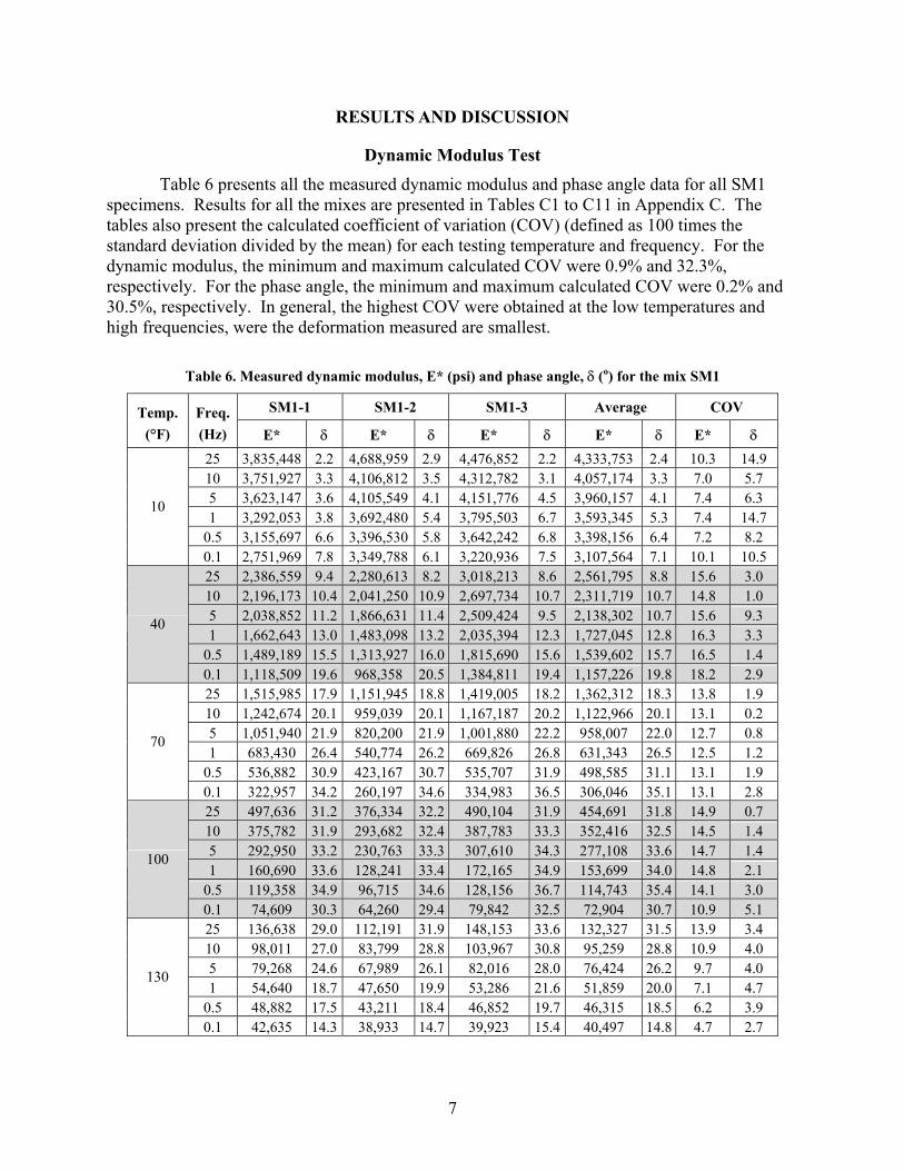
RESULTS AND DISCUSSION

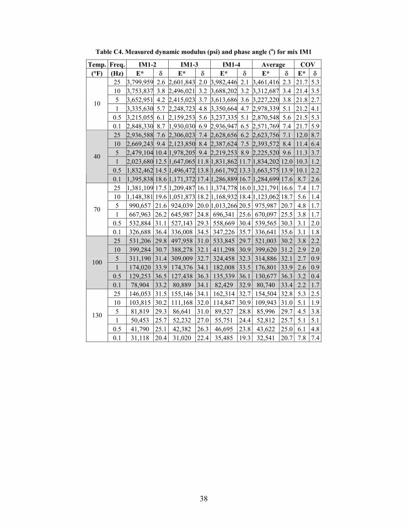
Dynamic Modulus Test Table 6 presents all the measured dynamic modulus and phase angle data for all SM1 specimens. Results for all the mixes are presented in Tables C1 to C11 in Appendix C. The tables also present the calculated coefficient of variation (COV) (defined as 100 times the standard deviation divided by the mean) for each testing temperature and frequency. For the dynamic modulus, the minimum and maximum calculated COV were 0.9% and 32.3%, respectively. For the phase angle, the minimum and maximum calculated COV were 0.2% and 30.5%, respectively. In general, the highest COV were obtained at the low temperatures and high frequencies, were the deformation measured are smallest.

Table 6. Measured dynamic modulus, E* (psi) and phase angle, δ (o) for the mix SM1

SM1-1 SM1-2 SM1-3 Average COV Temp. (°F)

Freq. (Hz) E* δ E* δ E* δ E* δ E* δ

25 3,835,448 2.2 4,688,959 2.9 4,476,852 2.2 4,333,753 2.4 10.3 14.9 10 3,751,927 3.3 4,106,812 3.5 4,312,782 3.1 4,057,174 3.3 7.0 5.7 5 3,623,147 3.6 4,105,549 4.1 4,151,776 4.5 3,960,157 4.1 7.4 6.3 1 3,292,053 3.8 3,692,480 5.4 3,795,503 6.7 3,593,345 5.3 7.4 14.7

0.5 3,155,697 6.6 3,396,530 5.8 3,642,242 6.8 3,398,156 6.4 7.2 8.2

10

0.1 2,751,969 7.8 3,349,788 6.1 3,220,936 7.5 3,107,564 7.1 10.1 10.5 25 2,386,559 9.4 2,280,613 8.2 3,018,213 8.6 2,561,795 8.8 15.6 3.0 10 2,196,173 10.4 2,041,250 10.9 2,697,734 10.7 2,311,719 10.7 14.8 1.0 5 2,038,852 11.2 1,866,631 11.4 2,509,424 9.5 2,138,302 10.7 15.6 9.3 1 1,662,643 13.0 1,483,098 13.2 2,035,394 12.3 1,727,045 12.8 16.3 3.3

0.5 1,489,189 15.5 1,313,927 16.0 1,815,690 15.6 1,539,602 15.7 16.5 1.4

40

0.1 1,118,509 19.6 968,358 20.5 1,384,811 19.4 1,157,226 19.8 18.2 2.9 25 1,515,985 17.9 1,151,945 18.8 1,419,005 18.2 1,362,312 18.3 13.8 1.9 10 1,242,674 20.1 959,039 20.1 1,167,187 20.2 1,122,966 20.1 13.1 0.2 5 1,051,940 21.9 820,200 21.9 1,001,880 22.2 958,007 22.0 12.7 0.8 1 683,430 26.4 540,774 26.2 669,826 26.8 631,343 26.5 12.5 1.2

0.5 536,882 30.9 423,167 30.7 535,707 31.9 498,585 31.1 13.1 1.9

70

0.1 322,957 34.2 260,197 34.6 334,983 36.5 306,046 35.1 13.1 2.8 25 497,636 31.2 376,334 32.2 490,104 31.9 454,691 31.8 14.9 0.7 10 375,782 31.9 293,682 32.4 387,783 33.3 352,416 32.5 14.5 1.4 5 292,950 33.2 230,763 33.3 307,610 34.3 277,108 33.6 14.7 1.4 1 160,690 33.6 128,241 33.4 172,165 34.9 153,699 34.0 14.8 2.1

0.5 119,358 34.9 96,715 34.6 128,156 36.7 114,743 35.4 14.1 3.0

100

0.1 74,609 30.3 64,260 29.4 79,842 32.5 72,904 30.7 10.9 5.1 25 136,638 29.0 112,191 31.9 148,153 33.6 132,327 31.5 13.9 3.4 10 98,011 27.0 83,799 28.8 103,967 30.8 95,259 28.8 10.9 4.0 5 79,268 24.6 67,989 26.1 82,016 28.0 76,424 26.2 9.7 4.0 1 54,640 18.7 47,650 19.9 53,286 21.6 51,859 20.0 7.1 4.7

0.5 48,882 17.5 43,211 18.4 46,852 19.7 46,315 18.5 6.2 3.9

130

0.1 42,635 14.3 38,933 14.7 39,923 15.4 40,497 14.8 4.7 2.7

8

Figure 2 shows the average measured dynamic modulus for mix SM1 as a function of frequency for each testing temperature. As expected, under a constant loading frequency, the magnitude of the dynamic modulus decreases with an increase in temperature; under a constant testing temperature, the magnitude of the dynamic modulus increases with an increase in the frequency. Figure 3 shows the measured phase angle results for the same mix.

1.E+04

1.E+05

1.E+06

1.E+07

0.01 0.1 1 10 100

Frequency (Hz)

|E*|

(psi

)

10°F 40°F 70°F 100°F 130°F

Figure 2. Dynamic modulus results for mix SM1

0

5

10

15

20

25

30

35

40

0.01 0.1 1 10 100

Frequency (Hz)

Phas

e an

gle

(°)

10°F 40°F 70°F 100°F 130°F

Figure 3. Phase angle results for mix SM1

9

Figure 3 shows that the phase angle decreases as the frequency increases at temperatures of 10°F, 40°F, and 70°F. However, at 100°F and 130°F, the behavior of the phase angle as a function of frequency is more complex. At 100°F, the phase angle seems to increase up to frequencies of 0.5 Hz, and then it starts to decrease as frequency increases. At 130°F, the phase angle increases with an increase in frequency. The complex behavior of the phase angle at higher temperatures or at lower frequencies could be attributed to the predominant effect of the aggregate interlock. This is in agreement with the findings of other researchers and previous testing in Virginia that reported that the elastic behavior of the aggregate dictates the response of the specimen at high temperatures and low frequencies (Flintsch et al., 2006; Clyne et al., 2003). Similar behavior was found for all other tested mixes.

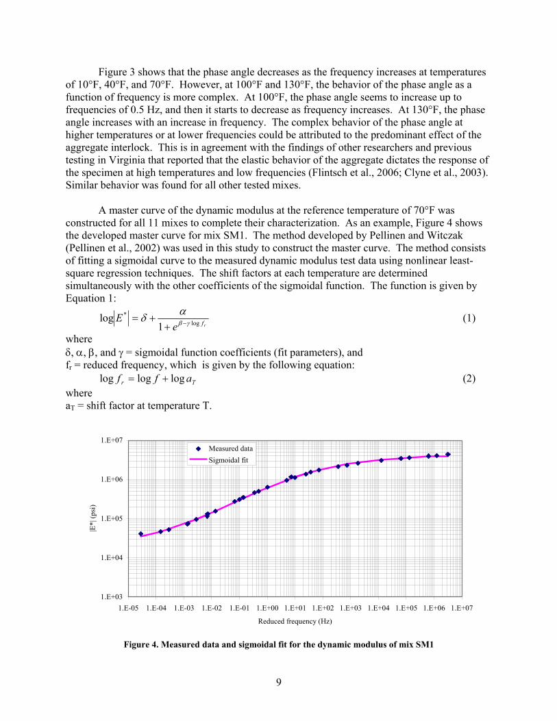
A master curve of the dynamic modulus at the reference temperature of 70°F was

constructed for all 11 mixes to complete their characterization. As an example, Figure 4 shows the developed master curve for mix SM1. The method developed by Pellinen and Witczak (Pellinen et al., 2002) was used in this study to construct the master curve. The method consists of fitting a sigmoidal curve to the measured dynamic modulus test data using nonlinear least-square regression techniques. The shift factors at each temperature are determined simultaneously with the other coefficients of the sigmoidal function. The function is given by Equation 1:

rfe

E log*

1log γβ

αδ −++= (1)

where δ, α, β, and γ = sigmoidal function coefficients (fit parameters), and fr = reduced frequency, which is given by the following equation: Tr aff logloglog += (2) where aT = shift factor at temperature T.

1.E+03

1.E+04

1.E+05

1.E+06

1.E+07

1.E-05 1.E-04 1.E-03 1.E-02 1.E-01 1.E+00 1.E+01 1.E+02 1.E+03 1.E+04 1.E+05 1.E+06 1.E+07

Reduced frequency (Hz)

|E*|

(psi

)

Measured dataSigmoidal fit

Figure 4. Measured data and sigmoidal fit for the dynamic modulus of mix SM1

10

The statistical software package SAS was used for the nonlinear regression analysis. Table 7 shows all the obtained sigmoidal function parameters and shift factors for all the mixes investigated. The parameters shown in Table 7 were used to construct and plot the master curves for all mixes in the frequency range of 10-5 Hz to 105 Hz. Figure 5 shows the developed master curves for all SM-9.5A mixes. From this plot, it is clear that mix SM3 exhibits the lowest dynamic modulus values at all frequencies. This can probably be explained by this mix having the highest asphalt content (6.3% as compared to 4.9% for mix SM1 and 5.9% for mix SM2) and on average 1% more voids than the other two mixes (see Table 5).

Table 7. Parameters of the measured dynamic modulus master curve for all mixes

Mix δ α β γ log(a10) log(a40) log(a70) log(a100) log(a130) SM1 4.23182 2.40375 -0.61155 0.5469 5.10729 1.86113 0 -1.86687 -3.5458 SM2 4.24358 2.34206 -0.52756 0.58509 4.60873 2.11614 0 -1.82198 -3.55407 SM3 3.96225 2.6038 -0.34476 0.5124 4.602 2.01282 0 -1.895 -3.47021 IM1 3.97617 2.59338 -0.89432 0.52568 4.55627 2.16329 0 -1.77346 -3.38386 IM2 4.1861 2.29254 -0.72547 0.57337 3.9556 2.03623 0 -1.77381 -3.36705 IM3 4.24285 2.41566 -0.7367 0.54358 4.99791 2.30204 0 -1.90961 -3.55711 IM4 4.25741 2.28306 -0.59524 0.63026 4.19403 2.34806 0 -1.899 -3.49271 BM1 4.10766 2.54327 -0.73887 0.49758 5.44215 2.03195 0 -1.93304 -3.51238 BM2 4.4979 2.2097 0.0689 0.55623 5.15319 2.20943 0 -1.85075 -3.44955 BM3 4.32085 2.33782 -1.14008 0.58795 4.9248 1.83275 0 -1.99614 -3.72051 BM4 4.07489 2.57073 -0.6343 0.51438 4.70522 2.18674 0 -1.85243 -3.43843

1.E+04

1.E+05

1.E+06

1.E+07

1.E-05 1.E-04 1.E-03 1.E-02 1.E-01 1.E+00 1.E+01 1.E+02 1.E+03 1.E+04 1.E+05

Reduced Frequency (Hz)

|E*|

(psi

)

SM1 SM2SM3

Figure 5. Dynamic modulus master curves for all SM-9.5A mixes

Figure 6 shows the developed master curves for all IM-19.0A mixes. This figure shows

that all the investigated IM mixes have similar dynamic modulus values at all frequencies, with mix IM3 having slightly higher values than the others.

11

1.E+04

1.E+05

1.E+06

1.E+07

1.E-05 1.E-04 1.E-03 1.E-02 1.E-01 1.E+00 1.E+01 1.E+02 1.E+03 1.E+04 1.E+05


|E*|

(psi

)IM1 IM2IM3 IM4

Figure 6. Dynamic modulus master curves for all IM-19.0A mixes

For the BM-25.0 mixes (Figure 7), mix BM3 exhibits the highest dynamic modulus

values at all frequencies while mix BM2 has the lowest dynamic modulus values at all frequencies. Mix BM3 has the lowest asphalt content (3.9%) while mix BM2 has the highest asphalt content (4.9%).

1.E+04

1.E+05

1.E+06

1.E+07

1.E-05 1.E-04 1.E-03 1.E-02 1.E-01 1.E+00 1.E+01 1.E+02 1.E+03 1.E+04 1.E+05


|E*|

(psi

)

BM1 BM2BM3 BM4

Figure 7. Dynamic modulus master curves for all BM-25.0 mixes

12

In addition, even though the JMF for mix BM2 reported the use the same binder than in the other BM mixes, the handling of the mix gave the impression that a different binder was used during production. The appearance of BM2 straight out of the box showed that the binder had concentrated in the bottom and had created what appeared to be splash marks on the box from where the material had been sampled. The mix was hard to compact, and after compaction the specimen remained spongy for a couple of hours with some small particles actually falling from the specimen. This abnormal behavior could also have been due to the absence of RAP in this mix.

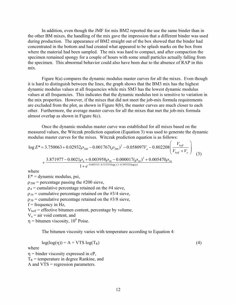
Figure 8(a) compares the dynamic modulus master curves for all the mixes. Even though

it is hard to distinguish between the lines, the graph shows that the BM3 mix has the highest dynamic modulus values at all frequencies while mix SM3 has the lowest dynamic modulus values at all frequencies. This indicates that the dynamic modulus test is sensitive to variation in the mix properties. However, if the mixes that did not meet the job-mix formula requirements are excluded from the plot, as shown in Figure 8(b), the master curves are much closer to each other. Furthermore, the average master curves for all the mixes that met the job-mix formula almost overlap as shown in Figure 8(c).

Once the dynamic modulus master curve was established for all mixes based on the

measured values, the Witczak prediction equation (Equation 3) was used to generate the dynamic modulus master curves for the mixes. Witczak prediction equation is as follows:

2200 200

24 38 38 34

0.603313 0.313351log( ) 0.393532log( )

log * 3.750063 0.02932 0.001767( ) 0.058097 0.802208

3.871977 0.0021 0.003958 0.000017( ) 0.0054701

beffa

beff a

f

VE V

V V

e η

ρ ρ

ρ ρ ρ ρ− − −

= + − − − +

− + − ++

+

(3)

where E* = dynamic modulus, psi, ρ200 = percentage passing the #200 sieve, ρ4 = cumulative percentage retained on the #4 sieve, ρ34 = cumulative percentage retained on the #3/4 sieve, ρ38 = cumulative percentage retained on the #3/8 sieve, f = frequency in Hz, Vbeff = effective bitumen content, percentage by volume, Va = air void content, and η = bitumen viscosity, 106 Poise.

The bitumen viscosity varies with temperature according to Equation 4: log(log(η)) = A + VTS log(TR) (4) where η = binder viscosity expressed in cP, TR = temperature in degree Rankine, and A and VTS = regression parameters.

13

1.E+04

1.E+05

1.E+06

1.E+07

1.E-05 1.E-04 1.E-03 1.E-02 1.E-01 1.E+00 1.E+01 1.E+02 1.E+03 1.E+04 1.E+05Reduced frequency (Hz)

|E*|

(psi

)

BM1 BM2 BM3 BM4

IM1 IM2 IM3 IM4

SM1 SM2 SM3

(a)

1.E+04

1.E+05

1.E+06

1.E+07


|E*|

(psi

)

BM1 BM2 BM4

IM2 IM3 IM4

SM1 SM2

(b)

1.E+04

1.E+05

1.E+06

1.E+07


|E*|

(psi

)

BM IM SM

(c)

Figure 8. Dynamic modulus master curves for (a) All mixes; (b) Excluding those that did not meet binder content specifications; and (c) Averages for those mixes meeting specifications

14

For this investigation, the default values suggested by the proposed MEPDG for a PG64-22 binder were used for all mixes. These default values are 10.98 for A and −3.68 for VTS. The sigmoidal function parameters and the shift factors were then determined for all the mixes and are presented in Table 8. The shift factors and the β and γ parameters are the same for all the mixes because the same values for A and VTS were used for all the mixes. This is a limitation since the master curve equation is sensitive to these parameters. It is recommended that these values be determined for each mix in future work rather than using the default values.

Table 8. Parameters of the predicted dynamic modulus master curve for all mixes

Mix δ α β γ log(a10) log(a40) log(a70) log(a100) log(a130) SM1 2.83869 3.81814 -0.99969 0.31361 4.29643 2.70454 0 -2.07415 -3.68771 SM2 2.83284 3.79412 -0.99969 0.31361 4.29643 2.70454 0 -2.07415 -3.68771 SM3 2.77352 3.80975 -0.99969 0.31361 4.29643 2.70454 0 -2.07415 -3.68771 IM1 2.8342 3.8179 -0.99969 0.31361 4.29643 2.70454 0 -2.07415 -3.68771 IM2 2.81245 3.8536 -0.99969 0.31361 4.29643 2.70454 0 -2.07415 -3.68771 IM3 2.81465 3.8801 -0.99969 0.31361 4.29643 2.70454 0 -2.07415 -3.68771 IM4 2.82705 3.87624 -0.99969 0.31361 4.29643 2.70454 0 -2.07415 -3.68771 BM1 2.80894 3.90252 -0.99969 0.31361 4.29643 2.70454 0 -2.07415 -3.68771 BM2 2.88335 4.00631 -0.99969 0.31361 4.29643 2.70454 0 -2.07415 -3.68771 BM3 2.87954 3.9466 -0.99969 0.31361 4.29643 2.70454 0 -2.07415 -3.68771 BM4 2.83202 3.87235 -0.99969 0.31361 4.29643 2.70454 0 -2.07415 -3.68771

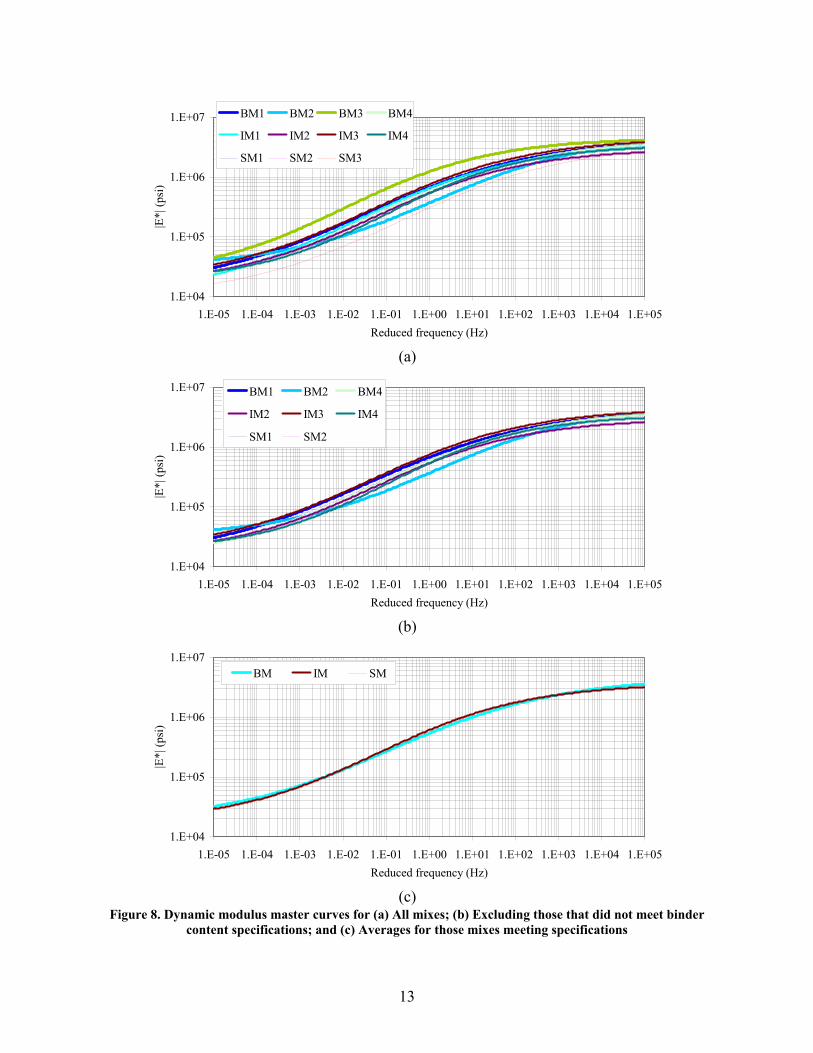
Figure 9 compares the measured and predicted master curves for mix SM1. For this

particular mix, the Witczak prediction equation underestimates the dynamic modulus at all frequencies; as shown by Figure 10, the ratio of the predicted to measured dynamic modulus varies between 0.5 and 0.9. This ratio varies from mix to mix. Table 9 presents the minimum and maximum values for this ratio for each mix. Since the predicted and measure values are close, level 2 input may be used with a reasonable degree of reliability.

1.E+04

1.E+05

1.E+06

1.E+07

1.E-05 1.E-04 1.E-03 1.E-02 1.E-01 1.E+00 1.E+01 1.E+02 1.E+03 1.E+04 1.E+05


|E*|

(psi

)

Measured Predicted

Figure 9. Measured and predicted dynamic modulus master curves for mix SM1

15

0

0.1

0.2

0.3

0.4

0.5

0.6

0.7

0.8

0.9

1

1.E-05 1.E-04 1.E-03 1.E-02 1.E-01 1.E+00 1.E+01 1.E+02 1.E+03 1.E+04 1.E+05

Reduced frequency (Hz)

|E*|

(pre

dict

ed) /

|E*|

(mea

sure

d)

Figure 10. Ratio of predicted to measured dynamic modulus for mix SM1

Table 9. Minimum and maximum values for the ratio of the predicted to measured dynamic modulus

Ratio SM1 SM2 SM3 IM1 IM2 IM3 IM4 BM1 BM2 BM3 BM4 Min. 0.54 0.58 0.75 0.60 0.60 0.48 0.64 0.54 0.52 0.45 0.68 Max. 0.90 1.07 1.56 0.90 1.01 0.75 1.24 0.80 1.90 0.84 1.05

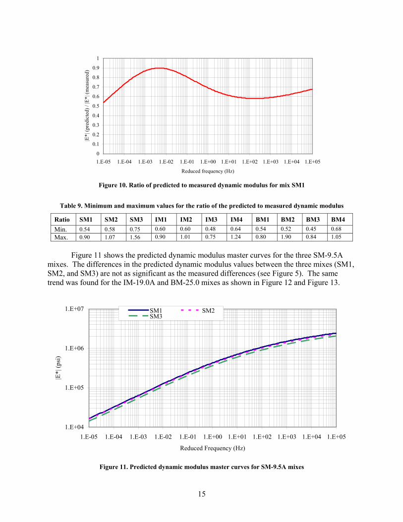
Figure 11 shows the predicted dynamic modulus master curves for the three SM-9.5A

mixes. The differences in the predicted dynamic modulus values between the three mixes (SM1, SM2, and SM3) are not as significant as the measured differences (see Figure 5). The same trend was found for the IM-19.0A and BM-25.0 mixes as shown in Figure 12 and Figure 13.

1.E+04

1.E+05

1.E+06

1.E+07

1.E-05 1.E-04 1.E-03 1.E-02 1.E-01 1.E+00 1.E+01 1.E+02 1.E+03 1.E+04 1.E+05


|E*|

(psi

)

SM1 SM2SM3

Figure 11. Predicted dynamic modulus master curves for SM-9.5A mixes

16

1.E+04

1.E+05

1.E+06

1.E+07

1.E-05 1.E-04 1.E-03 1.E-02 1.E-01 1.E+00 1.E+01 1.E+02 1.E+03 1.E+04 1.E+05


|E*|

(psi

)IM1 IM2

IM3 IM4

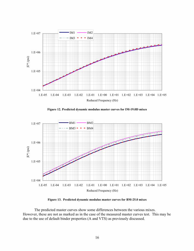
Figure 12. Predicted dynamic modulus master curves for IM-19.0D mixes

1.E+04

1.E+05

1.E+06

1.E+07

1.E-05 1.E-04 1.E-03 1.E-02 1.E-01 1.E+00 1.E+01 1.E+02 1.E+03 1.E+04 1.E+05


|E*|

(psi

)

BM1 BM2

BM3 BM4

Figure 13. Predicted dynamic modulus master curves for BM-25.0 mixes

The predicted master curves show some differences between the various mixes.

However, these are not as marked as in the case of the measured master curves test. This may be due to the use of default binder properties (A and VTS) as previously discussed.

17

Creep Test

The creep test results were used only in the low-temperature cracking model. In this project a master curve at a reference temperature of 32°F was determined for each tested specimen, and a power model was fit to the data to determine the slope parameter, m, which is required to compute several fracture (crack propagation) parameters in the fracture model of the MEPDG. The power model is defined by the following equation:

m

r 0 1 rD(t ) = D D t+ (4) where D(tr) = the creep compliance at the reduced time tr and D0, D1, and m = the power model parameters.

Figure 14 shows the developed master curve and its power model fit for specimen BM1-5A. It is important to note that several difficulties were encountered during the creep test. The data were not repeatable between specimens of the same mix, as can be seen in the obtained m values shown in Table 10. These problems are suspected to be due to the effect of the very low test temperature on the type of extensometers used. It is notable that five extensometers were damaged during the low-temperature creep tests. More problems were also encountered with mix BM2 as only one specimen could be tested. The other two prepared specimens broke during the testing.

0.01

0.1

1

0.001 0.01 0.1 1 10 100

Reduced Time (sec)

Com

plia

nce

(1/G

Pa)

Measured dataModel

Figure 14. Creep compliance master curve and power model fit for specimen BM1-5A

18

Table 10. m-parameter for all tested specimens

Mix Label m-value Mix Label m-value Mix Label m-value SM1-6A 0.45566 IM1-6A 0.37085 BM1-5A 0.37065 SM1-7B 0.19337 IM1-7A 0.43889 BM1-7A 0.33526 SM1

Avg. 0.324515 IM1

Avg. 0.40487 BM1

Avg. 0.352955 SM2-6A 0.36777 IM2-6A 0.34614 BM2-5B 0.46935 SM2-4B 0.52053 IM2-6B 0.29375 SM2

Avg. 0.44415 IM2

Avg. 0.319945 BM2

Avg. 0.46935 SM3-7A 0.7344 IM3-6B 0.19798 BM3-5A 0.37385 SM3-8B 0.40476 IM3-7A 0.34905 BM3-6B 0.18151 SM3

Avg. 0.56958 IM3

Avg. 0.273515 BM3

Avg. 0.27768 IM4-5A 0.35881 BM4-5A 0.21 IM4-6A 0.30452 BM4-6A 0.20983

IM4 Avg. 0.331665

BM4 Avg. 0.209915

Indirect Tensile Strength Test

The IDT strength at 14°F is also used in the low-temperature cracking model. The IDT tests for this investigation were conducted in the same specimens used for the creep test. Table 11 presents the results for all tested specimens.

Table 11. IDT strength results for all the mixes (ksi)

Mix Label Strength Mix Label Strength Mix Label Strength

SM1-6A 475 IM1-6A 420 BM1-5A 470

SM1-7B 499 IM1-7B 404 BM1-7A 392 SM1

Average 487

IM1

Average 412

BM1

Average 431

SM2-4B 477 IM2-6A 384 BM2-5B 354

SM2-5B 579 IM2-8B 424 SM2

Average 528

IM2

Average 404

BM2

Average 354

SM3-6A 409 IM3-6B 472 BM3-5A 479

SM3-7A 387 IM3-7A 463 BM2-6B 479 SM3

Average 398

IM3

Average 467

BM3

Average 479

IM4-6A 397 BM4-5A 415 IM4-7A 491 BM4-7B 367

IM4

Average 444

BM4

Average 393

19

Resilient Modulus Test

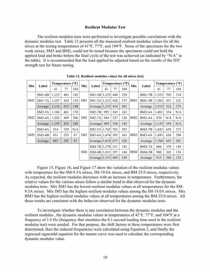
The resilient modulus tests were performed to investigate possible correlations with the dynamic modulus test. Table 12 presents all the measured resilient modulus values for all the mixes at the testing temperatures of 41°F, 77°F, and 104°F. Some of the specimens for the two weak mixes, SM3 and BM2, could not be tested because the specimens could not hold the applied load and broke before the final cycle of the test was achieved (as indicated by “N/A” in the table). It is recommended that the load applied be adjusted based on the results of the IDT strength test for future testing.

Table 12. Resilient modulus values for all mixes (ksi)

Temperature (°F) Temperature (°F) Temperature (°F)Mix Label

41 77 104 Mix Label

41 77 104 Mix Label

41 77 104

SM1-6B 1,125 401 142 IM1-5B 1,235 448 229 BM1-7B 1,523 592 318

SM1-7A 1,107 424 154 IM1-5A 1,231 420 173 BM1-5B 1,502 451 232 SM1

Average 1,116 412 148

IM1

Average 1,233 434 201

BM1

Average 1,513 522 275

SM2-5A 1,186 461 170 IM2-7B 995 345 163 BM2-6A 1,401 354 N/A

SM2-4A 1,203 449 206 IM2-7A 944 327 126 BM2-4A 870 N/A N/A SM2

Average 1,195 455 188

IM2

Average 969 336 145

BM2

Average 1,135 354 N/A

SM3-8A 914 329 N/A IM3-5A 1,765 762 293 BM3-7B 1,843 654 272

SM3-6B 851 255 87 IM3-6A 1,474 593 363 BM3-6A 1,693 656 290 SM3

Average 883 292 87

IM3

Average 1,619 677 328

BM3

Average 1,768 655 281

IM4-7B 1,270 531 143 BM4-7A 866 370 149 IM4-6B 1,031 397 144 BM4-5B 960 365 154 IM4

Average 1,151 464 144

BM4

Average 913 368 152

Figure 15, Figure 16, and Figure 17 show the variation of the resilient modulus values with temperature for the SM-9.5A mixes, IM-19.0A mixes, and BM-25.0 mixes, respectively. As expected, the resilient modulus decreases with an increase in temperature. Furthermore, the relative values for the various mixes follow a similar trend to that observed for the dynamic modulus tests. Mix SM3 has the lowest resilient modulus values at all temperatures for the SM-9.5A mixes. Mix IM3 has the highest resilient modulus values among the IM-19.0A mixes. Mix BM3 has the highest resilient modulus values at all temperatures among the BM-25.0 mixes. All these results are consistent with the behavior observed for the dynamic modulus tests. To investigate whether there is any correlation between the dynamic modulus and the resilient modulus , the dynamic modulus values at temperatures of 41°F, 77°F, and 104°F at a frequency of 1.6 Hz (frequency that simulates the 0.1-second loading time used in the resilient modulus test) were needed. For that purpose, the shift factors at these temperatures were first determined, then the reduced frequencies were calculated using Equation 2, and finally the regressed sigmoidal equation for the master curve was used to calculate the corresponding dynamic modulus value.

20

0

200

400

600

800

1000

1200

1400

40 50 60 70 80 90 100 110

Temperature (°F)

Res

ilien

t mod

ulus

(ksi

)SM1 SM2 SM3

Figure 15. Resilient modulus versus temperature for the SM-9.5A mixes

0

200

400

600

800

1000

1200

1400

1600

1800

40 50 60 70 80 90 100 110

Temperature (°F)

Res

ilien

t mod

ulus

(ksi

)

IM1 IM2 IM3 IM4

Figure 16. Resilient modulus versus temperature for the IM-19.0A mixes

21

0

200

400

600

800

1000

1200

1400

1600

1800

2000

40 50 60 70 80 90 100 110

Temperature (°F)

Res

ilien

t mod

ulus

(ksi

)BM1 BM2 BM3 BM4

Figure 17. Resilient modulus versus temperature for the BM-25.0 mixes

Figure 18 shows the resilient modulus versus the dynamic modulus for all mixes. This

figure shows that at low temperatures (high modulus values), the dynamic modulus is larger than the resilient modulus values, while at high temperatures (low modulus values), the values are closer to each other. The plots suggest that the relationship may not be linear and could possibly be mix dependent.

y = 1.53xR2 = 0.94

0

500

1000

1500

2000

2500

3000

0 500 1000 1500 2000 2500 3000

Resilient Modulus (ksi)

Dyn

amic

Mod

ulus

(ksi

)

Figure 18. Resilient modulus versus dynamic modulus for all mixes

22

To determine if there was a clear trend with temperature, the ratio of the dynamic modulus to the resilient modulus for all mixes was determined at all temperatures. Table 13 summarizes the values of this ratio. On average, the dynamic modulus value is 1.62 times the resilient modulus value at 41°F, 1.12 times the resilient modulus value at 77°F, and 0.88 times the resilient modulus value at 104°F. Furthermore, the ratio appears to be mix dependent.

These results suggest that if the resilient modulus values are used at low temperatures, the

prediction of the low-temperature cracking may be underestimated; if the resilient modulus values are used at high temperatures, the rutting prediction may also be underestimated.

Table 13. Ratio of dynamic modulus to resilient modulus for all mixes

Temperature (°F) Mix 41 77 104

SM1 1.80 0.90 0.65 SM2 1.53 0.78 0.46 SM3 1.41 0.95 1.04 IM1 1.60 1.56 1.23 IM2 1.58 1.40 1.00 IM3 1.51 0.93 0.55 IM4 1.70 1.22 1.27 BM1 1.43 0.98 0.58 BM2 1.44 0.70 N/A BM3 1.69 1.42 0.92 BM4 2.17 1.44 1.13

Average 1.62 1.12 0.88

FINDINGS

• As expected, under a constant loading frequency, the magnitude of the dynamic modulus decreases with an increase in temperature; under a constant testing temperature, the magnitude of the dynamic modulus increases with an increase in the frequency.

• The phase angle decreases as the frequency increases at testing temperatures of 10°F, 40°F, and 70°F. At 100°F, the phase angle seems to increase up to frequencies of 0.5 Hz, and then it starts to decrease with an increase in frequency. At 130°F, the phase angle increases with an increase in frequency.

• A sigmoidal function can be used for modeling the dynamic modulus data with very good statistical fit.

• Mixes of the same type (SM-9.5A, IM-19.0A, and BM-25.0) had different measured dynamic modulus values because they had different constituents (aggregate type, asphalt content, percentage RAP, etc.).

• The level 2 dynamic modulus prediction (Witczak) equation reasonably estimated the measured dynamic modulus. For all mixes, the ratio of the predicted to the measured

23

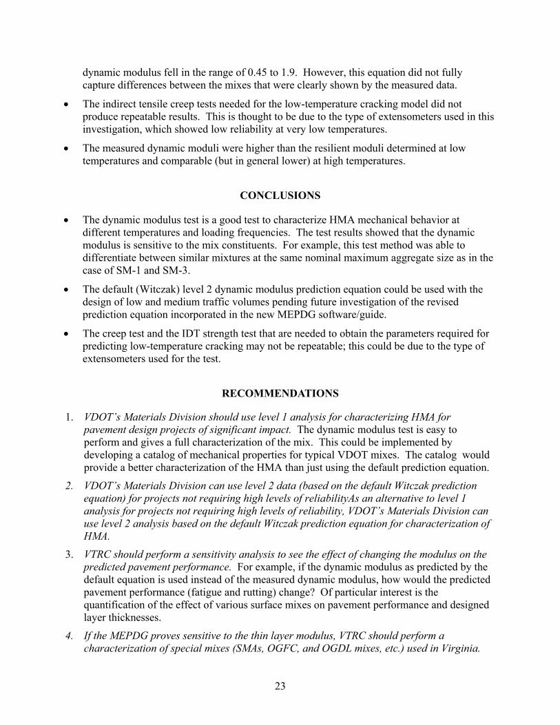
dynamic modulus fell in the range of 0.45 to 1.9. However, this equation did not fully capture differences between the mixes that were clearly shown by the measured data.

• The indirect tensile creep tests needed for the low-temperature cracking model did not produce repeatable results. This is thought to be due to the type of extensometers used in this investigation, which showed low reliability at very low temperatures.

• The measured dynamic moduli were higher than the resilient moduli determined at low temperatures and comparable (but in general lower) at high temperatures.

CONCLUSIONS

• The dynamic modulus test is a good test to characterize HMA mechanical behavior at different temperatures and loading frequencies. The test results showed that the dynamic modulus is sensitive to the mix constituents. For example, this test method was able to differentiate between similar mixtures at the same nominal maximum aggregate size as in the case of SM-1 and SM-3.

• The default (Witczak) level 2 dynamic modulus prediction equation could be used with the design of low and medium traffic volumes pending future investigation of the revised prediction equation incorporated in the new MEPDG software/guide.

• The creep test and the IDT strength test that are needed to obtain the parameters required for predicting low-temperature cracking may not be repeatable; this could be due to the type of extensometers used for the test.

RECOMMENDATIONS

1. VDOT’s Materials Division should use level 1 analysis for characterizing HMA for pavement design projects of significant impact. The dynamic modulus test is easy to perform and gives a full characterization of the mix. This could be implemented by developing a catalog of mechanical properties for typical VDOT mixes. The catalog would provide a better characterization of the HMA than just using the default prediction equation.

2. VDOT’s Materials Division can use level 2 data (based on the default Witczak prediction equation) for projects not requiring high levels of reliabilityAs an alternative to level 1 analysis for projects not requiring high levels of reliability, VDOT’s Materials Division can use level 2 analysis based on the default Witczak prediction equation for characterization of HMA.

3. VTRC should perform a sensitivity analysis to see the effect of changing the modulus on the predicted pavement performance. For example, if the dynamic modulus as predicted by the default equation is used instead of the measured dynamic modulus, how would the predicted pavement performance (fatigue and rutting) change? Of particular interest is the quantification of the effect of various surface mixes on pavement performance and designed layer thicknesses.

4. If the MEPDG proves sensitive to the thin layer modulus, VTRC should perform a characterization of special mixes (SMAs, OGFC, and OGDL mixes, etc.) used in Virginia.

24

COSTS AND BENEFITS ASSESSMENT

The results of this study directly support implementation efforts currently underway to initiate statewide usage of the proposed MEPDG. The characterization findings provide necessary inputs for the design guide. Use of the design guide is expected to improve the efficiency of asphalt pavement designs and result in more accurate predictions of maintenance and rehabilitation needs over the life of the asphalt pavement. This will allow for more economical scheduling practices to optimize maintenance strategies. Cost savings of these efficiencies cannot be directly calculated at this time, as they must be determined at either the project or network level; such determination is beyond the scope of this study. However, these savings are expected to be significant when applied to the almost 58,000 miles of roadways that are maintained by VDOT considerable mileage of HMA-surfaced pavements that are maintained by VDOT. .

ACKNOWLEDGMENTS

The authors acknowledge the contribution of the following individuals to the successful completion of the project: Troy Deeds, VTRC; Billy Hobbs, Samer Katicha, and Zheng Wu, VTTI; and the project review panel: Bill Maupin, VTRC; Mohamed Elfino, Mourad Bouhajja, and Haroon Shami, VDOT; Richard Schreck, Virginia Asphalt Association; and Lorenzo Casanova, Federal Highway Administration.

REFERENCES

Clyne, T.R., Li, X., Marasteanu, M.O., and Skok, E.L. Dynamic and Resilient Modulus of MN DOT Asphalt Mixtures. MN/RC-2003-09. Minnesota Department of Transportation, Minneapolis, 2003.

Federal Highway Administration Design Guide Implementation Team, American Association of State Highways and Transportation Officials. AASHTO TP62-03, Asphalt Material Properties: AC Mixture Inputs—Mix Stiffness, Workshop on Materials Input for Mechanistic-Empirical Pavement Design. Thornburg, VA, 2005.

Flintsch, G.W., Al-Qadi, I.L., Loulizi, A., and Mokarem, D. Laboratory Tests for Hot-Mix Asphalt Characterization in Virginia. VTRC 05-CR22. Virginia Transportation Research Council, Charlottesville, 2005.

Pellinen, T.K., and Witczak, M.W. Stress Dependent Master Curve Construction for Dynamic Modulus. Journal of the Association of Asphalt Paving Technologists, Vol. 71, 2002, pp. 281-309.

25

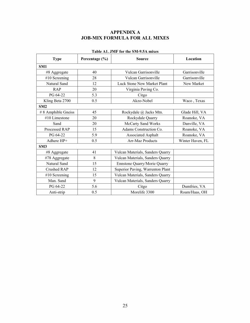
APPENDIX A JOB-MIX FORMULA FOR ALL MIXES

Table A1. JMF for the SM-9.5A mixes

Type Percentage (%) Source Location

SM1 #8 Aggregate 40 Vulcan Garrisonville Garrisonville #10 Screening 28 Vulcan Garrisonville Garrisonville Natural Sand 12 Luck Stone New Market Plant New Market

RAP 20 Virginia Paving Co. PG 64-22 5.3 Citgo

Kling Beta 2700 0.5 Akzo-Nobel Waco , Texas SM2 # 8 Amphible Gneiss 45 Rockydale @ Jacks Mtn. Glade Hill, VA

#10 Limestone 20 Rockydale Quarry Roanoke, VA Sand 20 McCarty Sand Works Danville, VA

Processed RAP 15 Adams Construction Co. Roanoke, VA PG 64-22 5.9 Associated Asphalt Roanoke, VA

Adhere HP+ 0.5 Arr-Maz Products Winter Haven, FL SM3

#8 Aggregate 41 Vulcan Materials, Sanders Quarry #78 Aggregate 8 Vulcan Materials, Sanders Quarry Natural Sand 15 Ennstone Quarry/Morie Quarry Crushed RAP 12 Superior Paving, Warrenton Plant #10 Screening 15 Vulcan Materials, Sanders Quarry

Man. Sand 9 Vulcan Materials, Sanders Quarry PG 64-22 5.6 Citgo Dumfries, VA Anti-strip 0.5 Morelife 3300 Roam/Haas, OH

26

Table A2. JMF for the IM-19.0 mixes


IM1 #8 Aggregate 21 Vulcan Materials Lorton, VA #68 Aggregate 30 Vulcan Materials Lorton, VA

Man. Sand 19 Vulcan Materials Lorton, VA Natural Sand 10 Mid Atlantic King George, VA

½-inch Recl. RAP 20 APAC, Inc. Occoquan, VA PG 64-22 4.6 Citgo Dumfries, VA

Adhere HP+ 0.5 Arr-Maz Products Winter Haven, FL IM2

#67 Aggregate 35 Vulcan Materials #8 Aggregate 25 Vulcan Materials

Sand 20 Vulcan Materials RAP 20 Branscome

PG 64-22 4.6 Kock Fuels Inc. Adhere HP+ 0.3 Arr-Maz Products Winter Haven, FL

IM3 #68 Limestone 50 Boxley Rich Patch, VA #10 Limestone 25 Boxley Rich Patch, VA

Sand 5 Brett Aggregates Inc. Stuart Draft, VA Processed RAP 20 Adams Construction Co. Lowmoore, VA

PG 64-22 4.9 Associated Asphalt, Inc. Roanoke, VA Adhere HP+ 0.5 Arr-Maz Products Winter Haven, FL

IM4 #68 Limestone 47 Luck Stone Staunton, VA #8 Limestone 10 Luck Stone Staunton, VA

#10 Limestone 32 Luck Stone Staunton, VA Sand 10 DM Conner Stuarts Drafts, VA Lime 1 Greer Lime Riverton, WV

PG 64-22 5.5 Associated Asphalt Roanoke, VA

27

Table A3. JMF for the BM-25.0 mixes


BM1 #5 Aggregate 22 Vulcan Garrisonville #68 Aggregate 27 Vulcan Garrisonville Natural sand 10 Luck Stone New Market

#10 screening 16 Vulcan Garrisonville RAP millings 25 Virginia Paving Co.

PG 64-22 4.4 Citgo Kling Beta 2700 0.5 Akzo-Nobel Waco , Texas

BM2 #8 Limestone 32 Stuart M. Perry Inc. Winchester

#56 Limestone 30 Stuart M. Perry Inc. Winchester #10 Limestone 30 Stuart M. Perry Inc. Winchester

Sand 8 Stuart M. Perry Inc. Winchester PG 64-22 4.9 Citgo Asphalt Refining Dumfries, VA

Kling Beta 2700 0.5 Citgo Asphalt Refining Dumfries, VA BM3 #357 Limestone 18 Acco Stone Blacksburg, VA #68 Limestone 30 Acco Stone Blacksburg, VA #10 Limestone 27 Acco Stone Blacksburg, VA Concrete Sand 10 Wythe Sand Co. Wytheville, VA Processed RAP 15 Adams Construction Co. Blacksburg, VA

PG 64-22 4.4 Associated Asphalt, Inc. Roanoke, VA Adhere HP+ 0.5 Arr-Maz Products Winter Haven, FL

BM4 #67 Aggregate 15 Vulcan Materials #8 Aggregate 15 Vulcan Materials #5 Aggregate 28 Vulcan Materials

Sand 27 Vulcan Materials RAP 15 Branscome Inc.

PG 64-22 4.4 Koch Fuels Inc. Adhere HP+ 0.5 Arr-Maz Products Winter Haven, FL

29

APPENDIX B ASPHALT CONTENT, Gmm, AND GRADATION FOR ALL MIXES

Table B1. Asphalt content, Gmm, and aggregate gradation for SM1 Sample 1 Sample 2 Sample 3 Sample 4 Average JMF* Acceptance

Asphalt content (%) 4.99 4.84 5.06 4.82 4.93 5.3 5.0-5.6 Gmm 2.635 2.633 2.630 2.622 2.630 2.626

Gradation Acceptance range*


% Passing Sample 1

% Passing Sample 2

% Passing Sample 3

% Passing Sample 4

% Passing Avg. Lower

limit Upper limit

12.5 (1/2) 96.6 97.3 97.8 97.9 97.4 - 100 9.5 (3/8) 886 88.7 91.5 90.6 89.9 89 97 4.75 (#4) 55.6 55.7 59.5 57.1 57.2 56 64 2.36 (#8) 37.3 37.1 39.2 37.8 37.9 36 44

1.18 (#16) 27.6 27.4 28.6 27.8 27.9 - - 0.6 (#30) 19.2 19.1 19.9 19.4 19.4 - - 0.3 (#50) 10.8 10.7 11.2 10.9 10.9 - -

0.15 (#100) 6.7 6.7 7.1 6.8 6.8 - - 0.075 (#200) 4.9 4.9 5.2 5.0 5.0 4 6

*Reported from the JMF sheet

Table B2. Asphalt content, Gmm, and aggregate gradation for SM2

Sample 1 Sample 2 Sample 3 Sample 4 Average JMF* Acceptance Asphalt content (%) 5.98 6.01 5.85 5.79 5.91 5.9 5.6-6.2

Gmm 2.669 2.632 2.642 2.651 2.648 2.618 Gradation

Acceptance range* Sieve opening, mm

(No.) % Passing Sample 1

% Passing Sample 2

% Passing Sample 3

% Passing Sample 4


limit Upper limit

12.5 (1/2) 100.0 100.0 100.0 100.0 100.0 99 100 9.5 (3/8) 94.5 96.9 96.7 97.1 96.3 92 100 4.75 (#4) 53.9 58.1 59.2 57.5 57.1 56 64 2.36 (#8) 36.0 38.0 38.7 37.7 37.6 37 45

1.18 (#16) 27.4 28.2 28.8 28.3 28.1 - - 0.6 (#30) 19.8 20.1 20.7 20.3 20.2 - - 0.3 (#50) 12.7 12.5 13.1 12.8 12.8 - -

0.15 (#100) 8.6 8.2 8.7 8.5 8.5 - - 0.075 (#200) 6.5 5.8 6.4 6.3 6.3 4.9 6.9


30

Table B3. Asphalt content, Gmm, and aggregate gradation for SM3


Gmm 2.597 2.593 2.591 2.605 2.596 2.599 Gradation



% Passing Sample 2

% Passing Sample 3

% Passing Sample 4


limit Upper limit

12.5 (1/2) 99.5 99.7 99.2 98.5 99.2 99 100 9.5 (3/8) 91.1 90.3 92.8 91.6 91.4 89 97 4.75 (#4) 55.2 55.8 57.3 54.8 55.8 55 63 2.36 (#8) 39.4 39.9 40.4 38.5 39.5 36 44

1.18 (#16) 29.8 30.1 30.7 29.4 30.0 - - 0.6 (#30) 21.3 21.5 21.9 21.0 21.5 - - 0.3 (#50) 13.3 13.5 13.7 13.2 13.4 - -

0.15 (#100) 9.0 9.2 9.2 9.0 9.1 - - 0.075 (#200) 6.1 6.3 6.4 6.3 6.3 4.7 6.7


Table B4. Asphalt content, Gmm, and aggregate gradation for IM1


Gmm 2.480 2.482 2.468 2.477 2.477 2.504 Gradation



% Passing Sample 2

% Passing Sample 3

% Passing Sample 4


limit Upper limit

25 (1) 100.0 100.0 100.0 100.0 100.0 - 100 19 (3/4) 100.0 100.0 100.0 100.0 100.0 92 100

12.5 (1/2) 97.1 94.9 96.0 95.0 95.8 84 92 9.5 (3/8) 88.0 86.9 88.3 86.9 87.5 - - 4.75 (#4) 53.5 53.9 54.4 50.4 53.0 - - 2.36 (#8) 37.7 38.3 38.5 36.5 37.7 29 37

1.18 (#16) 29.4 29.7 29.8 28.6 29.4 - - 0.6 (#30) 21.9 22.0 22.0 21.4 21.8 - - 0.3 (#50) 14.5 14.7 14.6 14.3 14.5 - -

0.15 (#100) 9.8 10.0 9.8 9.8 9.9 - - 0.075 (#200) 6.5 6.8 6.6 6.7 6.6 4.0 6.0


31



Gmm 2.512 2.510 2.511 2.521 2.513 2.500 Gradation



% Passing Sample 2

% Passing Sample 3

% Passing Sample 4


limit Upper limit

25 (1) 100.0 100.0 100.0 100.0 100.0 - 100 19 (3/4) 100.0 97.8 95.0 97.7 97.6 92 100

12.5 (1/2) 85.4 86.0 82.6 84.3 84.6 80 88 9.5 (3/8) 74.2 73.9 70.9 74.1 73.3 - - 4.75 (#4) 41.8 40.7 41.1 42.2 41.5 - - 2.36 (#8) 29.8 29.3 29.9 30.0 29.8 29 37

1.18 (#16) 24.4 24.0 24.2 24.4 24.2 - - 0.6 (#30) 18.3 18.0 18.0 18.3 18.1 - - 0.3 (#50) 11.6 11.4 11.4 11.6 11.5 - -

0.15 (#100) 6.7 6.5 6.5 6.7 6.6 - - 0.075 (#200) 3.9 3.7 3.8 3.9 3.8 3.4 5.4




Gmm 2.533 2.516 2.523 2.523 2.524 Gradation



% Passing Sample 2

% Passing Sample 3

% Passing Sample 4


limit Upper limit

25 (1) 100.0 100.0 100.0 100.0 100.0 - 100 19 (3/4) 96.3 97.4 93.7 98.3 96.4 92 100

12.5 (1/2) 75.6 83.3 79.8 80.6 79.8 76 84 9.5 (3/8) 66.3 73.9 69.0 68.6 69.5 - - 4.75 (#4) 42.7 48.7 45.5 45.6 45.6 - - 2.36 (#8) 28.7 32.3 30.4 30.1 30.4 28 36

1.18 (#16) 20.1 22.2 21.2 21.0 21.1 - - 0.6 (#30) 14.7 16.2 15.5 15.4 15.4 - - 0.3 (#50) 10.0 10.9 10.5 10.4 10.4 - -

0.15 (#100) 7.0 7.5 7.3 7.2 7.2 - - 0.075 (#200) 5.3 5.6 5.5 5.4 5.5 4.0 6.0


32



Gmm 2.489 2.489 2.486 2.481 2.486 2.502 Gradation



% Passing Sample 2

% Passing Sample 3

% Passing Sample 4


limit Upper limit

25 (1) 100.0 100.0 100.0 100.0 100.0 - 100 19 (3/4) 98.6 98.3 98.1 100.0 98.8 92 100

12.5 (1/2) 85.0 85.6 83.4 87.1 85.3 82 90 9.5 (3/8) 75.8 74.7 72.8 78.3 75.4 - - 4.75 (#4) 57.8 58.2 56.6 61.5 58.5 - - 2.36 (#8) 39.4 39.6 39.1 41.9 40.0 26 34

1.18 (#16) 30.0 30.1 29.7 31.4 30.3 - - 0.6 (#30) 23.2 23.3 23.0 24.2 23.4 - - 0.3 (#50) 14.3 14.3 14.1 14.7 14.4 - -

0.15 (#100) 8.1 8.0 7.9 8.2 8.0 - - 0.075 (#200) 6.0 5.9 5.8 6.0 5.9 4.0 6.0


Table B8. Asphalt content, Gmm, and aggregate gradation for BM1


Gmm 2.690 2.692 2.698 2.685 2.691 2.668 Gradation



% Passing Sample 2

% Passing Sample 3

% Passing Sample 4


limit Upper limit

37.5 (1.5) 100.0 100.0 100.0 100.0 100.0 100 25 (1) 100.0 100.0 98.5 98.2 99.2 92 100

19 (3/4) 95.3 97.4 92.3 92.6 94.4 82 90 12.5 (1/2) 77.9 76.8 72.2 76.7 75.9 - - 9.5 (3/8) 67.8 65.6 62.8 67.7 66.0 - - 4.75 (#4) 47.9 46.4 43.6 47.2 46.3 - - 2.36 (#8) 32.3 31.5 29.7 31.9 31.3 26 34

1.18 (#16) 23.5 23.2 22.0 23.4 23.0 - - 0.6 (#30) 16.9 16.6 15.9 16.8 16.6 - - 0.3 (#50) 10.8 10.6 10.2 10.8 10.6 - -

0.15 (#100) 7.5 7.3 7.1 7.5 7.4 - - 0.075 (#200) 5.6 5.4 5.2 5.6 5.4 3.0 5.0


33



Gmm 2.493 2.522 2.504 2.519 2.509 2.515 Gradation



% Passing Sample 2

% Passing Sample 3

% Passing Sample 4


limit Upper limit

37.5 (1.5) 100.0 100.0 100.0 100.0 100.0 100 25 (1) 82.5 83.7 82.4 87.8 84.1 90 98

19 (3/4) 73.6 71.4 75.4 74.9 73.8 73 81 12.5 (1/2) 71.2 66.1 70.8 70.4 69.6 - - 9.5 (3/8) 67.8 63.8 67.5 67.5 66.6 - - 4.75 (#4) 43.5 41.5 44.2 42.5 42.9 - - 2.36 (#8) 26.8 25.7 27.2 26.3 26.5 25 33

1.18 (#16) 17.3 16.3 17.6 16.8 17.0 - - 0.6 (#30) 11.6 10.9 11.9 11.2 11.4 - - 0.3 (#50) 8.4 7.8 8.6 8.0 8.2 - -

0.15 (#100) 6.7 6.2 7.0 6.3 6.5 - - 0.075 (#200) 5.5 5.2 5.9 5.2 5.5 3.6 5.6




Gmm 2.646 2.638 2.645 2.631 2.640 2.605 Gradation



% Passing Sample 2

% Passing Sample 3

% Passing Sample 4


limit Upper limit

37.5 (1.5) 100.0 100.0 100.0 100.0 100.0 100 25 (1) 95.8 100.0 96.2 97.2 97.3 90 98

19 (3/4) 87.4 87.6 86.7 88.8 87.6 82 90 12.5 (1/2) 72.6 72.9 72.1 75.7 73.3 - - 9.5 (3/8) 64.6 63.7 62.4 68.3 64.8 - - 4.75 (#4) 46.1 47.3 47.6 50.9 48.0 - - 2.36 (#8) 23.6 24.2 23.5 25.4 24.2 25 33

1.18 (#16) 16.8 17.2 16.8 17.8 17.1 - - 0.6 (#30) 12.9 13.1 13.0 13.6 13.1 - - 0.3 (#50) 8.7 8.8 8.8 9.2 8.9 - -

0.15 (#100) 7.0 7.0 7.0 7.3 7.1 - - 0.075 (#200) 6.0 6.0 6.0 6.3 6.1 4.0 6.0


34



Gmm 2.506 2.514 2.520 2.525 2.516 2.525 Gradation



% Passing Sample 2

% Passing Sample 3

% Passing Sample 4


limit Upper limit

37.5 (1.5) 100.0 100.0 100.0 100.0 100.0 100 25 (1) 100.0 100.0 100.0 100.0 100.0 92 100

19 (3/4) 95.5 96.1 95.6 94.6 95.5 81 89 12.5 (1/2) 85.0 80.8 82.7 81.4 82.5 - - 9.5 (3/8) 73.2 68.7 70.5 69.8 70.6 - - 4.75 (#4) 42.4 40.9 41.5 39.6 41.1 - - 2.36 (#8) 31.2 30.2 30.7 29.3 30.3 33 41

1.18 (#16) 25.2 24.6 24.8 24.0 24.7 - - 0.6 (#30) 18.5 18.1 18.2 17.9 18.2 - - 0.3 (#50) 11.1 10.9 10.9 10.9 11.0 - -

0.15 (#100) 6.3 6.2 6.2 6.3 6.2 - - 0.075 (#200) 3.9 3.8 3.8 4.0 3.9 3.2 5.2


35

APPENDIX C MEASURED DYNAMIC MODULUS RESULTS

Table C1. Measured dynamic modulus (psi) and phase angle (o) for mix SM1

Temp. Freq. SM1-1 SM1-2 SM1-3 Average COV (°F) (Hz) E* δ E* δ E* δ E* δ E* δ

25 3,835,448 2.2 4,688,959 2.9 4,476,852 2.2 4,333,753 2.4 10.3 14.9 10 3,751,927 3.3 4,106,812 3.5 4,312,782 3.1 4,057,174 3.3 7.0 5.7 5 3,623,147 3.6 4,105,549 4.1 4,151,776 4.5 3,960,157 4.1 7.4 6.3 1 3,292,053 3.8 3,692,480 5.4 3,795,503 6.7 3,593,345 5.3 7.4 14.7

0.5 3,155,697 6.6 3,396,530 5.8 3,642,242 6.8 3,398,156 6.4 7.2 8.2

10

0.1 2,751,969 7.8 3,349,788 6.1 3,220,936 7.5 3,107,564 7.1 10.1 10.5 25 2,386,559 9.4 2,280,613 8.2 3,018,213 8.6 2,561,795 8.8 15.6 3.0 10 2,196,173 10.4 2,041,250 10.9 2,697,734 10.7 2,311,719 10.7 14.8 1.0 5 2,038,852 11.2 1,866,631 11.4 2,509,424 9.5 2,138,302 10.7 15.6 9.3 1 1,662,643 13.0 1,483,098 13.2 2,035,394 12.3 1,727,045 12.8 16.3 3.3

0.5 1,489,189 15.5 1,313,927 16.0 1,815,690 15.6 1,539,602 15.7 16.5 1.4

40

0.1 1,118,509 19.6 968,358 20.5 1,384,811 19.4 1,157,226 19.8 18.2 2.9 25 1,515,985 17.9 1,151,945 18.8 1,419,005 18.2 1,362,312 18.3 13.8 1.9 10 1,242,674 20.1 959,039 20.1 1,167,187 20.2 1,122,966 20.1 13.1 0.2 5 1,051,940 21.9 820,200 21.9 1,001,880 22.2 958,007 22.0 12.7 0.8 1 683,430 26.4 540,774 26.2 669,826 26.8 631,343 26.5 12.5 1.2

0.5 536,882 30.9 423,167 30.7 535,707 31.9 498,585 31.1 13.1 1.9

70

0.1 322,957 34.2 260,197 34.6 334,983 36.5 306,046 35.1 13.1 2.8 25 497,636 31.2 376,334 32.2 490,104 31.9 454,691 31.8 14.9 0.7 10 375,782 31.9 293,682 32.4 387,783 33.3 352,416 32.5 14.5 1.4 5 292,950 33.2 230,763 33.3 307,610 34.3 277,108 33.6 14.7 1.4 1 160,690 33.6 128,241 33.4 172,165 34.9 153,699 34.0 14.8 2.1

0.5 119,358 34.9 96,715 34.6 128,156 36.7 114,743 35.4 14.1 3.0

100

0.1 74,609 30.3 64,260 29.4 79,842 32.5 72,904 30.7 10.9 5.1 25 136,638 29.0 112,191 31.9 148,153 33.6 132,327 31.5 13.9 3.4 10 98,011 27.0 83,799 28.8 103,967 30.8 95,259 28.8 10.9 4.0 5 79,268 24.6 67,989 26.1 82,016 28.0 76,424 26.2 9.7 4.0 1 54,640 18.7 47,650 19.9 53,286 21.6 51,859 20.0 7.1 4.7

0.5 48,882 17.5 43,211 18.4 46,852 19.7 46,315 18.5 6.2 3.9

130

0.1 42,635 14.3 38,933 14.7 39,923 15.4 40,497 14.8 4.7 2.7

36



25 3,361,675 2.7 3,853,492 2.2 3,900,886 2.5 3,705,351 2.5 8.1 7.4 10 3,119,653 3.5 3,605,338 4.1 3,776,419 3.6 3,500,470 3.7 9.7 7.6 5 2,975,516 4.2 3,440,721 4.8 3,673,327 3.9 3,363,188 4.3 10.6 10.9 1 2,891,353 5.8 3,201,201 5.9 3,303,212 4.8 3,131,922 5.5 6.8 9.8

0.5 2,835,376 6.5 3,053,679 6.4 3,274,504 5.5 3,054,520 6.2 7.2 7.6

10

0.1 2,377,251 8.6 2,717,761 6.8 2,717,750 7.8 2,604,254 7.7 7.5 7.4 25 2,692,772 7.9 2,733,359 7.0 2,391,087 7.3 2,605,739 7.4 7.2 2.8 10 2,435,325 8.8 2,473,170 10.7 2,139,470 9.9 2,349,322 9.8 7.8 5.1 5 2,206,687 11.7 2,273,719 10.9 1,986,331 11.2 2,155,579 11.2 7.0 1.9 1 1,788,554 14.5 1,830,099 14.8 1,586,363 14.0 1,735,005 14.5 7.5 2.8

0.5 1,584,017 16.8 1,604,446 17.9 1,423,560 18.0 1,537,341 17.6 6.4 1.3

40

0.1 1,145,724 23.2 1,203,918 21.9 1,042,206 21.8 1,130,616 22.3 7.2 1.2 25 1,245,189 19.4 1,202,700 19.3 1,143,550 19.8 1,197,146 19.5 4.3 1.4 10 1,008,604 21.9 997,219 22.0 939,208 22.1 981,677 22.0 3.8 0.4 5 851,962 24.4 851,258 24.1 794,911 24.3 832,710 24.3 3.9 0.5 1 546,002 29.6 552,658 29.4 512,563 29.6 537,074 29.6 4.0 0.4

0.5 421,218 34.6 430,229 34.7 398,904 34.9 416,784 34.8 3.9 0.2

70

0.1 250,352 38.1 259,003 37.8 239,780 38.1 249,712 38.0 3.9 0.5 25 369,309 33.4 375,195 34.3 447,021 33.7 397,175 33.8 10.9 0.9 10 268,965 33.5 280,337 34.5 325,518 33.9 291,607 34.0 10.3 1.0 5 204,861 34.0 215,984 34.5 249,150 34.1 223,332 34.2 10.3 0.6 1 112,268 31.6 118,099 32.2 137,892 31.8 122,753 31.9 10.9 0.7

0.5 87,110 31.8 91,483 32.1 108,427 31.5 95,673 31.8 11.8 0.9

100

0.1 57,925 26.3 59,823 26.4 74,060 25.7 63,936 26.1 13.8 1.3 25 98,187 29.4 118,232 27.8 93,799 29.7 103,406 28.9 12.6 3.3 10 73,442 25.8 86,912 25.5 68,876 26.9 76,410 26.1 12.3 2.6 5 60,440 23.6 70,988 23.4 56,187 24.4 62,538 23.8 12.2 2.2 1 43,126 18.4 49,601 18.9 38,936 19.4 43,888 18.9 12.2 1.5

0.5 38,922 17.4 44,204 18.1 34,144 18.3 39,090 17.9 12.9 0.9

130

0.1 34,194 15.3 37,633 16.4 28,866 15.4 33,564 15.7 13.2 3.2

37



25 2,983,947 3.3 3,159,968 3.5 3,212,086 3.7 3,118,667 3.5 3.8 4.2 10 2,774,559 4.9 3,044,689 4.9 3,077,795 5.4 2,965,681 5.1 5.6 4.9 5 2,645,241 6.0 2,914,124 5.6 2,954,835 6.1 2,838,067 5.9 5.9 3.9 1 2,336,639 7.7 2,580,539 7.1 2,608,025 7.7 2,508,401 7.5 6.0 4.4

0.5 2,189,525 8.7 2,443,996 8.6 2,459,759 8.8 2,364,427 8.7 6.4 1.1

10

0.1 1,839,427 11.4 2,069,365 10.3 2,087,677 11.3 1,998,823 11.0 6.9 4.5 25 1,745,398 10.4 1,938,607 10.8 1,886,781 10.9 1,856,929 10.7 5.4 0.8 10 1,537,887 13.4 1,694,713 11.8 1,656,442 12.7 1,629,681 12.6 5.0 4.0 5 1,379,286 16.0 1,521,620 13.5 1,499,349 14.6 1,466,752 14.7 5.2 4.5 1 1,015,539 19.8 1,167,131 17.7 1,132,291 18.3 1,104,987 18.6 7.2 2.5

0.5 864,401 22.7 1,006,109 21.1 970,848 22.1 947,119 22.0 7.8 2.6

40

0.1 580,466 29.2 682,960 26.4 659,131 27.8 640,852 27.8 8.4 2.9 25 754,173 25.0 815,983 22.6 792,607 24.9 787,588 24.2 4.0 4.9 10 596,386 27.4 650,060 25.1 630,115 26.0 625,520 26.2 4.3 2.2 5 488,170 29.4 535,729 27.1 515,923 28.0 513,274 28.1 4.7 2.1 1 293,147 32.9 325,934 31.4 311,024 31.7 310,035 32.0 5.3 1.0

0.5 221,368 36.9 247,073 35.2 237,512 35.7 235,317 36.0 5.5 1.0

70

0.1 134,660 36.5 150,171 35.3 144,582 34.9 143,138 35.6 5.5 1.0 25 190,047 32.6 223,707 31.5 238,863 33.2 217,539 32.4 11.5 2.6 10 136,541 31.3 156,512 31.1 170,240 31.7 154,431 31.4 11.0 1.0 5 107,558 30.3 122,935 30.5 131,664 30.7 120,719 30.5 10.1 0.3 1 64,815 26.2 73,274 27.3 77,425 26.7 71,838 26.7 8.9 1.2

0.5 52,956 25.5 58,729 27.3 62,641 26.1 58,109 26.3 8.4 2.5

100

0.1 38,697 21.7 41,710 23.4 45,375 22.1 41,927 22.4 8.0 3.0 25 64,192 24.3 70,470 27.9 70,362 27.1 68,341 26.4 5.3 2.9 10 48,012 22.3 51,133 24.3 51,209 23.0 50,118 23.2 3.6 2.9 5 38,509 21.2 42,767 22.6 42,418 21.5 41,232 21.8 5.7 2.5 1 27,409 17.8 28,355 19.2 30,054 17.1 28,606 18.0 4.7 5.7

0.5 23,437 19.0 24,216 19.2 26,723 17.3 24,792 18.5 6.9 5.2

130

0.1 18,070 16.8 18,920 16.9 22,475 15.2 19,822 16.3 11.8 5.1

38

Table C4. Measured dynamic modulus (psi) and phase angle (o) for mix IM1

Temp. Freq. IM1-2 IM1-3 IM1-4 Average COV (°F) (Hz) E* δ E* δ E* δ E* δ E* δ

25 3,799,959 2.6 2,601,843 2.0 3,982,446 2.1 3,461,416 2.3 21.7 5.3 10 3,753,837 3.8 2,496,021 3.2 3,688,202 3.2 3,312,687 3.4 21.4 3.5 5 3,652,951 4.2 2,415,023 3.7 3,613,686 3.6 3,227,220 3.8 21.8 2.7 1 3,335,630 5.7 2,248,723 4.8 3,350,664 4.7 2,978,339 5.1 21.2 4.1

0.5 3,215,055 6.1 2,159,253 5.6 3,237,335 5.1 2,870,548 5.6 21.5 5.3

10

0.1 2,848,330 8.7 1,930,030 6.9 2,936,947 6.5 2,571,769 7.4 21.7 5.9 25 2,936,588 7.6 2,306,023 7.4 2,628,656 6.2 2,623,756 7.1 12.0 8.7 10 2,669,243 9.4 2,123,850 8.4 2,387,624 7.5 2,393,572 8.4 11.4 6.4 5 2,479,104 10.4 1,978,205 9.4 2,219,253 8.9 2,225,520 9.6 11.3 3.7 1 2,023,680 12.5 1,647,065 11.8 1,831,862 11.7 1,834,202 12.0 10.3 1.2

0.5 1,832,462 14.5 1,496,472 13.8 1,661,792 13.3 1,663,575 13.9 10.1 2.2

40

0.1 1,395,838 18.6 1,171,372 17.4 1,286,889 16.7 1,284,699 17.6 8.7 2.6 25 1,381,109 17.5 1,209,487 16.1 1,374,778 16.0 1,321,791 16.6 7.4 1.7 10 1,148,381 19.6 1,051,873 18.2 1,168,932 18.4 1,123,062 18.7 5.6 1.4 5 990,657 21.6 924,039 20.0 1,013,266 20.5 975,987 20.7 4.8 1.7 1 667,963 26.2 645,987 24.8 696,341 25.6 670,097 25.5 3.8 1.7

0.5 532,884 31.1 527,143 29.3 558,669 30.4 539,565 30.3 3.1 2.0

70

0.1 326,688 36.4 336,008 34.5 347,226 35.7 336,641 35.6 3.1 1.8 25 531,206 29.8 497,958 31.0 533,845 29.7 521,003 30.2 3.8 2.2 10 399,284 30.7 388,278 32.1 411,298 30.9 399,620 31.2 2.9 2.0 5 311,190 31.4 309,009 32.7 324,458 32.3 314,886 32.1 2.7 0.9 1 174,020 33.9 174,376 34.1 182,008 33.5 176,801 33.9 2.6 0.9

0.5 129,253 36.5 127,438 36.3 135,339 36.1 130,677 36.3 3.2 0.4

100

0.1 78,904 33.2 80,889 34.1 82,429 32.9 80,740 33.4 2.2 1.7 25 146,053 31.5 155,146 34.1 162,314 32.7 154,504 32.8 5.3 2.5 10 103,815 30.2 111,168 32.0 114,847 30.9 109,943 31.0 5.1 1.9 5 81,819 29.3 86,641 31.0 89,527 28.8 85,996 29.7 4.5 3.8 1 50,453 25.7 52,232 27.0 55,751 24.4 52,812 25.7 5.1 5.1

0.5 41,790 25.1 42,382 26.3 46,695 23.8 43,622 25.0 6.1 4.8

130

0.1 31,118 20.4 31,020 22.4 35,485 19.3 32,541 20.7 7.8 7.4

39



25 2,605,963 1.9 3,033,936 1.6 2,806,081 1.8 2,815,327 1.8 7.6 6.1 10 2,447,338 3.3 2,843,993 3.9 2,636,216 3.6 2,642,516 3.6 7.5 5.1 5 2,358,315 3.9 2,728,723 4.4 2,538,667 4.5 2,541,902 4.3 7.3 2.4 1 2,152,103 4.9 2,481,817 5.4 2,300,639 5.8 2,311,520 5.4 7.1 4.1

0.5 2,046,140 6.3 2,357,737 6.4 2,192,267 6.4 2,198,715 6.4 7.1 0.4

10

0.1 1,814,534 8.0 2,102,922 8.1 1,949,646 8.1 1,955,701 8.1 7.4 0.3 25 2,128,822 6.9 2,079,287 8.0 2,283,495 8.4 2,163,868 7.7 4.9 4.2 10 1,953,805 9.3 1,883,446 9.4 2,068,485 9.4 1,968,579 9.4 4.7 0.3 5 1,805,862 10.7 1,745,094 10.9 1,923,983 10.5 1,824,980 10.7 5.0 1.5 1 1,477,836 13.6 1,426,612 13.6 1,557,069 13.3 1,487,172 13.5 4.4 1.2

0.5 1,326,630 16.0 1,282,367 16.0 1,402,179 15.8 1,337,059 15.9 4.5 0.6

40

0.1 1,005,749 20.5 989,641 21.0 1,060,961 20.6 1,018,784 20.7 3.7 1.0 25 1,164,844 17.7 1,039,816 17.9 1,159,003 17.7 1,121,221 17.8 6.3 0.6 10 981,247 20.6 892,251 19.5 990,120 20.2 954,540 20.1 5.7 1.8 5 838,401 22.7 772,477 21.4 851,263 22.4 820,714 22.2 5.1 2.3 1 556,741 27.5 526,349 25.9 564,424 27.6 549,171 27.0 3.7 3.1

0.5 438,200 32.0 419,561 30.7 442,962 32.5 433,575 31.7 2.9 2.9

70

0.1 273,853 34.6 266,525 34.0 275,763 35.8 272,047 34.8 1.8 2.5 25 431,713 29.4 408,029 29.7 427,375 30.5 422,372 29.9 3.0 1.5 10 325,805 30.1 310,328 29.9 329,354 31.1 321,829 30.3 3.1 2.0 5 257,763 31.1 245,458 30.6 257,528 32.3 253,583 31.3 2.8 2.8 1 149,487 30.3 140,355 30.1 145,038 31.9 144,960 30.8 3.2 3.0

0.5 116,629 31.2 106,821 31.2 110,680 33.3 111,376 31.9 4.4 3.4

100

0.1 77,841 27.3 70,007 27.3 70,706 28.5 72,851 27.7 6.0 2.2 25 131,571 29.7 131,743 28.7 138,224 31.0 133,846 29.8 2.8 3.9 10 95,559 27.4 94,123 27.2 95,565 29.1 95,082 27.9 0.9 3.4 5 75,952 25.1 74,372 25.6 75,673 27.6 75,332 26.1 1.1 3.9 1 52,245 19.6 49,839 20.7 48,044 22.4 50,043 20.9 4.2 4.3

0.5 46,451 18.6 43,082 19.4 40,782 21.4 43,438 19.8 6.6 5.4

130

0.1 37,988 15.8 36,192 15.2 31,357 18.3 35,179 16.4 9.7 9.5

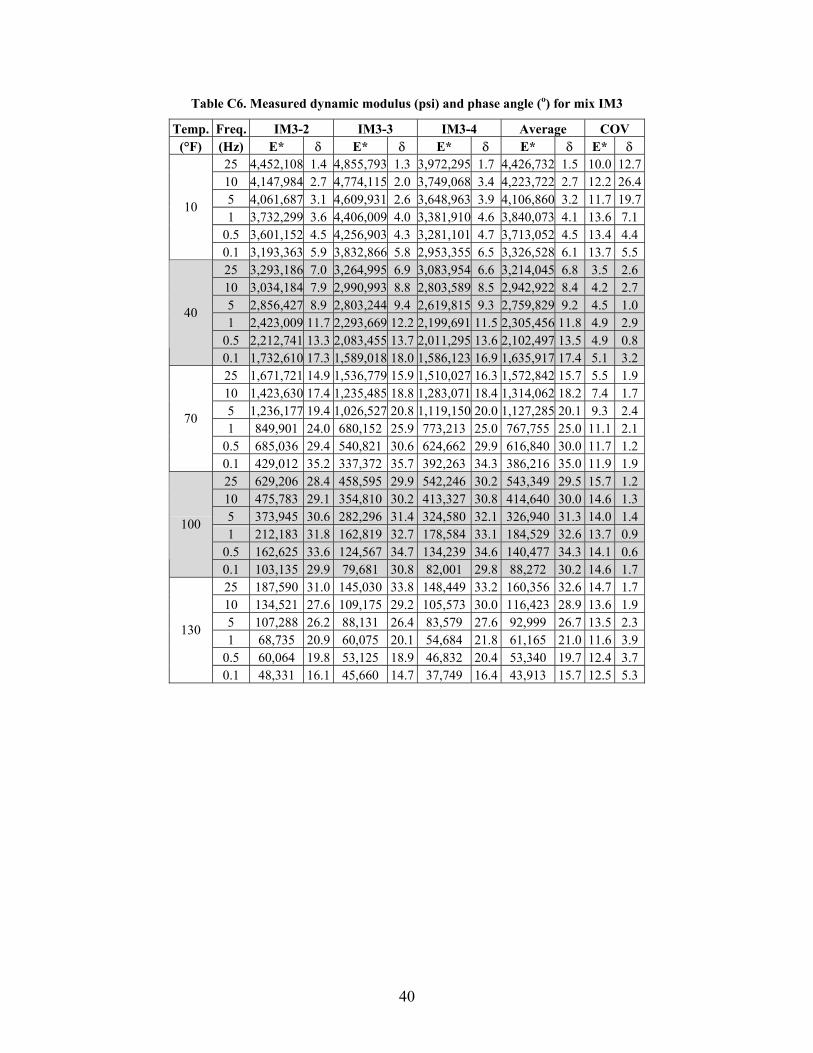
40



25 4,452,108 1.4 4,855,793 1.3 3,972,295 1.7 4,426,732 1.5 10.0 12.7 10 4,147,984 2.7 4,774,115 2.0 3,749,068 3.4 4,223,722 2.7 12.2 26.4 5 4,061,687 3.1 4,609,931 2.6 3,648,963 3.9 4,106,860 3.2 11.7 19.7 1 3,732,299 3.6 4,406,009 4.0 3,381,910 4.6 3,840,073 4.1 13.6 7.1

0.5 3,601,152 4.5 4,256,903 4.3 3,281,101 4.7 3,713,052 4.5 13.4 4.4

10

0.1 3,193,363 5.9 3,832,866 5.8 2,953,355 6.5 3,326,528 6.1 13.7 5.5 25 3,293,186 7.0 3,264,995 6.9 3,083,954 6.6 3,214,045 6.8 3.5 2.6 10 3,034,184 7.9 2,990,993 8.8 2,803,589 8.5 2,942,922 8.4 4.2 2.7 5 2,856,427 8.9 2,803,244 9.4 2,619,815 9.3 2,759,829 9.2 4.5 1.0 1 2,423,009 11.7 2,293,669 12.2 2,199,691 11.5 2,305,456 11.8 4.9 2.9

0.5 2,212,741 13.3 2,083,455 13.7 2,011,295 13.6 2,102,497 13.5 4.9 0.8

40

0.1 1,732,610 17.3 1,589,018 18.0 1,586,123 16.9 1,635,917 17.4 5.1 3.2 25 1,671,721 14.9 1,536,779 15.9 1,510,027 16.3 1,572,842 15.7 5.5 1.9 10 1,423,630 17.4 1,235,485 18.8 1,283,071 18.4 1,314,062 18.2 7.4 1.7 5 1,236,177 19.4 1,026,527 20.8 1,119,150 20.0 1,127,285 20.1 9.3 2.4 1 849,901 24.0 680,152 25.9 773,213 25.0 767,755 25.0 11.1 2.1

0.5 685,036 29.4 540,821 30.6 624,662 29.9 616,840 30.0 11.7 1.2

70

0.1 429,012 35.2 337,372 35.7 392,263 34.3 386,216 35.0 11.9 1.9 25 629,206 28.4 458,595 29.9 542,246 30.2 543,349 29.5 15.7 1.2 10 475,783 29.1 354,810 30.2 413,327 30.8 414,640 30.0 14.6 1.3 5 373,945 30.6 282,296 31.4 324,580 32.1 326,940 31.3 14.0 1.4 1 212,183 31.8 162,819 32.7 178,584 33.1 184,529 32.6 13.7 0.9

0.5 162,625 33.6 124,567 34.7 134,239 34.6 140,477 34.3 14.1 0.6

100

0.1 103,135 29.9 79,681 30.8 82,001 29.8 88,272 30.2 14.6 1.7 25 187,590 31.0 145,030 33.8 148,449 33.2 160,356 32.6 14.7 1.7 10 134,521 27.6 109,175 29.2 105,573 30.0 116,423 28.9 13.6 1.9 5 107,288 26.2 88,131 26.4 83,579 27.6 92,999 26.7 13.5 2.3 1 68,735 20.9 60,075 20.1 54,684 21.8 61,165 21.0 11.6 3.9

0.5 60,064 19.8 53,125 18.9 46,832 20.4 53,340 19.7 12.4 3.7

130

0.1 48,331 16.1 45,660 14.7 37,749 16.4 43,913 15.7 12.5 5.3

41



25 2,657,970 2.3 2,812,233 2.7 4,580,072 1.7 3,350,092 2.2 31.9 22.9 10 2,475,741 3.6 2,644,419 4.1 4,164,395 3.1 3,094,851 3.6 30.1 13.7 5 2,419,100 4.0 2,567,555 4.2 4,045,120 4.1 3,010,592 4.1 29.9 1.8 1 2,233,736 4.8 2,407,288 5.2 3,709,436 4.7 2,783,487 4.9 29.0 5.9

0.5 2,143,259 5.7 2,322,889 5.8 3,573,326 5.7 2,679,825 5.7 29.1 1.2

10

0.1 1,925,529 7.5 2,105,238 7.3 3,390,296 7.5 2,473,688 7.4 32.3 1.3 25 2,643,782 5.4 2,429,997 8.2 3,321,266 4.5 2,798,348 6.0 16.6 30.5 10 2,407,619 8.9 2,214,430 9.9 2,965,105 8.0 2,529,051 8.9 15.4 10.7 5 2,232,901 10.4 2,044,376 10.9 2,731,903 9.2 2,336,393 10.2 15.2 8.1 1 1,833,855 13.3 1,667,274 13.6 2,211,338 12.6 1,904,156 13.1 14.6 3.7

0.5 1,651,763 15.3 1,507,748 16.4 1,975,491 15.0 1,711,667 15.6 14.0 4.4

40

0.1 1,237,071 20.6 1,125,176 21.5 1,466,763 19.4 1,276,337 20.5 13.6 5.1 25 1,285,329 18.1 1,141,262 19.3 1,240,421 18.5 1,222,337 18.6 6.0 2.1 10 1,073,681 20.4 940,392 21.4 1,009,489 21.4 1,007,854 21.0 6.6 1.0 5 912,361 22.4 799,226 23.9 857,114 23.5 856,234 23.3 6.6 1.4 1 586,279 28.4 512,119 29.6 554,227 28.7 550,875 28.9 6.8 1.5

0.5 457,702 34.0 395,819 34.7 432,541 33.5 428,687 34.1 7.3 1.6

70

0.1 264,301 37.6 232,494 38.1 259,250 37.3 252,015 37.6 6.8 1.0 25 392,634 33.2 320,708 33.3 416,349 32.6 376,564 33.0 13.2 1.1 10 284,060 33.4 229,886 33.5 303,165 33.6 272,370 33.5 14.0 0.1 5 216,991 33.7 174,849 33.6 228,749 34.3 206,863 33.9 13.7 1.1 1 120,020 31.5 95,694 30.8 122,776 33.2 112,830 31.8 13.2 3.9

0.5 93,060 31.3 74,265 30.2 92,747 33.2 86,691 31.6 12.4 4.8

100

0.1 62,819 25.4 50,296 24.1 60,531 27.4 57,882 25.6 11.5 6.4 25 106,757 27.8 88,874 29.6 118,890 30.3 104,840 29.2 14.4 1.8 10 77,808 24.6 62,763 26.3 83,239 27.7 74,603 26.2 14.2 3.3 5 63,655 22.4 50,928 23.7 66,665 25.3 60,416 23.8 13.8 3.8 1 46,059 17.2 36,741 17.9 45,635 19.7 42,812 18.3 12.3 5.0

0.5 40,996 16.4 32,916 17.3 39,905 18.9 37,939 17.5 11.6 4.8

130

0.1 34,751 14.3 28,956 14.9 33,278 16.5 32,328 15.2 9.3 5.6

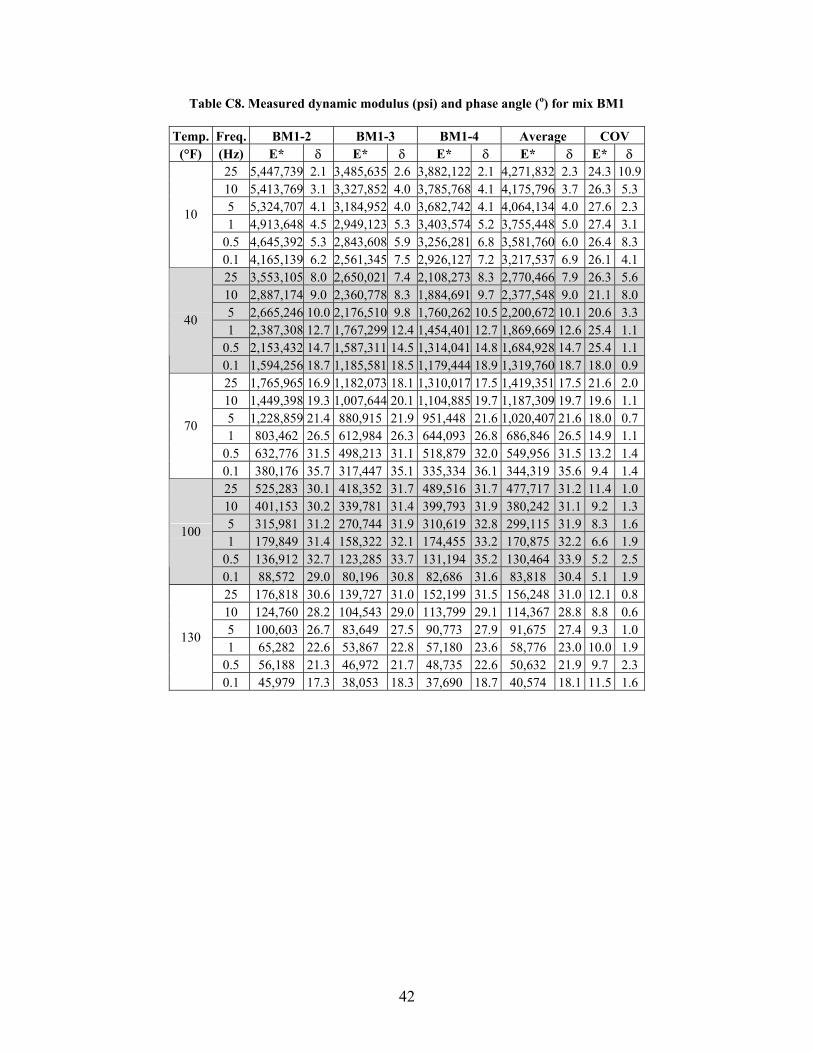
42

Table C8. Measured dynamic modulus (psi) and phase angle (o) for mix BM1

Temp. Freq. BM1-2 BM1-3 BM1-4 Average COV (°F) (Hz) E* δ E* δ E* δ E* δ E* δ

25 5,447,739 2.1 3,485,635 2.6 3,882,122 2.1 4,271,832 2.3 24.3 10.9 10 5,413,769 3.1 3,327,852 4.0 3,785,768 4.1 4,175,796 3.7 26.3 5.3 5 5,324,707 4.1 3,184,952 4.0 3,682,742 4.1 4,064,134 4.0 27.6 2.3 1 4,913,648 4.5 2,949,123 5.3 3,403,574 5.2 3,755,448 5.0 27.4 3.1

0.5 4,645,392 5.3 2,843,608 5.9 3,256,281 6.8 3,581,760 6.0 26.4 8.3

10

0.1 4,165,139 6.2 2,561,345 7.5 2,926,127 7.2 3,217,537 6.9 26.1 4.1 25 3,553,105 8.0 2,650,021 7.4 2,108,273 8.3 2,770,466 7.9 26.3 5.6 10 2,887,174 9.0 2,360,778 8.3 1,884,691 9.7 2,377,548 9.0 21.1 8.0 5 2,665,246 10.0 2,176,510 9.8 1,760,262 10.5 2,200,672 10.1 20.6 3.3 1 2,387,308 12.7 1,767,299 12.4 1,454,401 12.7 1,869,669 12.6 25.4 1.1

0.5 2,153,432 14.7 1,587,311 14.5 1,314,041 14.8 1,684,928 14.7 25.4 1.1

40

0.1 1,594,256 18.7 1,185,581 18.5 1,179,444 18.9 1,319,760 18.7 18.0 0.9 25 1,765,965 16.9 1,182,073 18.1 1,310,017 17.5 1,419,351 17.5 21.6 2.0 10 1,449,398 19.3 1,007,644 20.1 1,104,885 19.7 1,187,309 19.7 19.6 1.1 5 1,228,859 21.4 880,915 21.9 951,448 21.6 1,020,407 21.6 18.0 0.7 1 803,462 26.5 612,984 26.3 644,093 26.8 686,846 26.5 14.9 1.1

0.5 632,776 31.5 498,213 31.1 518,879 32.0 549,956 31.5 13.2 1.4

70

0.1 380,176 35.7 317,447 35.1 335,334 36.1 344,319 35.6 9.4 1.4 25 525,283 30.1 418,352 31.7 489,516 31.7 477,717 31.2 11.4 1.0 10 401,153 30.2 339,781 31.4 399,793 31.9 380,242 31.1 9.2 1.3 5 315,981 31.2 270,744 31.9 310,619 32.8 299,115 31.9 8.3 1.6 1 179,849 31.4 158,322 32.1 174,455 33.2 170,875 32.2 6.6 1.9

0.5 136,912 32.7 123,285 33.7 131,194 35.2 130,464 33.9 5.2 2.5

100

0.1 88,572 29.0 80,196 30.8 82,686 31.6 83,818 30.4 5.1 1.9 25 176,818 30.6 139,727 31.0 152,199 31.5 156,248 31.0 12.1 0.8 10 124,760 28.2 104,543 29.0 113,799 29.1 114,367 28.8 8.8 0.6 5 100,603 26.7 83,649 27.5 90,773 27.9 91,675 27.4 9.3 1.0 1 65,282 22.6 53,867 22.8 57,180 23.6 58,776 23.0 10.0 1.9

0.5 56,188 21.3 46,972 21.7 48,735 22.6 50,632 21.9 9.7 2.3

130

0.1 45,979 17.3 38,053 18.3 37,690 18.7 40,574 18.1 11.5 1.6

43



25 4,651,571 2.1 4,714,695 2.3 4,267,176 3.0 4,544,481 2.5 5.3 15.2 10 4,518,000 5.1 4,526,405 4.5 4,190,307 5.4 4,411,571 5.0 4.3 9.7 5 4,367,265 5.8 4,342,129 5.2 4,021,055 5.5 4,243,483 5.5 4.5 3.1 1 3,858,460 6.5 4,074,193 5.8 3,633,689 8.0 3,855,447 6.8 5.7 16.5

0.5 3,685,568 7.6 3,873,692 7.7 3,401,185 8.6 3,653,482 8.0 6.5 5.4

10

0.1 3,170,742 9.9 3,319,661 9.8 2,534,385 10.6 3,008,263 10.1 13.9 3.8 25 2,549,444 8.7 2,656,520 10.1 2,428,547 9.7 2,544,837 9.5 4.5 3.1 10 2,213,821 12.0 2,342,522 10.9 2,130,873 12.4 2,229,072 11.7 4.8 6.4 5 2,003,846 13.9 2,150,109 13.9 1,959,750 13.6 2,037,902 13.8 4.9 1.0 1 1,524,369 17.1 1,623,750 17.3 1,495,662 17.2 1,547,927 17.2 4.3 0.3

0.5 1,294,042 20.4 1,379,798 20.7 1,259,423 22.2 1,311,087 21.1 4.7 3.8

40

0.1 870,244 27.2 919,171 28.5 846,866 28.5 878,760 28.1 4.2 0.9 25 911,738 24.2 921,885 23.0 971,132 23.2 934,918 23.5 3.4 1.0 10 727,513 25.9 725,356 25.6 782,963 24.7 745,277 25.4 4.4 1.8 5 599,049 27.9 590,919 27.6 654,171 26.4 614,713 27.3 5.6 2.4 1 365,923 31.5 356,618 31.6 404,076 30.2 375,539 31.1 6.7 2.3

0.5 284,493 35.5 273,293 35.5 313,885 34.0 290,557 35.0 7.2 2.1

70

0.1 177,334 35.4 167,309 35.6 198,888 35.2 181,177 35.4 8.9 0.6 25 263,263 32.2 268,881 32.2 312,267 29.8 281,470 31.4 9.5 4.0 10 191,351 30.2 200,622 29.4 228,510 28.7 206,827 29.4 9.4 1.5 5 152,247 28.5 160,347 27.7 183,511 26.8 165,368 27.7 9.8 1.8 1 97,052 23.4 104,271 22.7 120,186 21.7 107,170 22.6 11.0 2.4

0.5 82,578 22.4 89,528 21.6 104,784 20.1 92,297 21.4 12.3 3.7

100

0.1 64,200 18.8 70,283 18.0 87,139 16.1 73,874 17.6 16.1 5.6 25 85,700 24.1 101,687 28.9 130,659 21.7 106,016 24.9 21.5 14.5 10 69,581 21.1 76,132 24.5 99,583 17.9 81,765 21.2 19.3 15.6 5 59,519 19.4 65,951 20.6 86,538 15.4 70,669 18.4 20.0 14.3 1 44,679 15.6 56,015 15.2 71,538 10.5 57,411 13.8 23.5 17.7

0.5 39,750 16.2 52,816 16.2 68,337 10.5 53,635 14.3 26.7 20.3

130

0.1 31,541 16.7 45,642 18.3 66,560 14.8 47,915 16.6 36.8 10.5

44



25 3,905,150 1.0 4,500,290 1.2 5,846,646 0.7 4,750,695 1.0 20.9 25.8 10 3,700,068 2.8 4,299,523 2.9 5,799,677 2.8 4,599,756 2.8 23.5 2.3 5 3,611,326 3.0 4,166,157 3.2 5,656,177 3.0 4,477,887 3.1 23.6 4.4 1 3,378,276 4.0 3,879,639 4.3 5,246,119 4.4 4,168,011 4.2 23.2 2.1

0.5 3,278,735 4.5 3,721,678 4.6 5,089,470 4.6 4,029,961 4.6 23.4 0.9

10

0.1 3,034,728 5.4 3,383,135 5.6 4,565,363 6.0 3,661,075 5.6 21.9 3.4 25 3,326,260 6.1 2,918,242 7.0 3,740,895 5.9 3,328,466 6.3 12.4 8.2 10 3,132,914 7.6 2,694,654 8.3 3,467,443 7.1 3,098,337 7.6 12.5 8.0 5 2,962,230 8.3 2,552,201 9.0 3,266,949 7.6 2,927,127 8.3 12.3 8.4 1 2,512,802 10.7 2,169,892 11.4 2,792,918 9.5 2,491,871 10.5 12.5 8.8

0.5 2,786,871 12.3 1,979,919 12.9 3,065,746 11.4 2,610,845 12.2 21.6 6.1

40

0.1 2,219,083 15.6 1,581,851 16.9 2,401,845 14.4 2,067,593 15.6 20.8 7.9 25 2,478,302 14.6 2,451,896 16.4 2,118,546 14.6 2,349,581 15.2 8.5 6.1 10 2,154,928 16.1 2,131,138 18.0 1,812,104 16.7 2,032,723 16.9 9.4 4.0 5 1,890,333 17.8 1,873,017 19.9 1,590,944 18.7 1,784,765 18.8 9.4 3.6 1 1,324,571 23.4 1,303,774 25.0 1,114,390 23.9 1,247,578 24.1 9.3 2.4

0.5 1,074,409 28.5 1,061,624 30.1 909,894 29.0 1,015,309 29.2 9.0 2.0

70

0.1 675,622 35.0 655,186 34.6 580,895 34.7 637,234 34.7 7.8 0.2 25 949,573 27.0 756,416 27.9 889,094 27.7 865,027 27.5 11.4 0.7 10 719,699 29.0 577,747 29.2 666,049 29.1 654,499 29.1 11.0 0.2 5 575,496 30.9 455,777 31.2 530,107 31.1 520,460 31.1 11.6 0.2 1 326,092 34.0 256,419 32.8 301,151 32.7 294,554 33.2 12.0 0.8

0.5 244,189 37.4 193,379 35.2 228,570 34.9 222,046 35.8 11.7 1.3

100

0.1 147,025 36.0 115,953 32.0 144,868 32.3 135,949 33.4 12.8 2.3 25 255,963 33.0 196,535 34.4 257,083 31.4 236,527 32.9 14.6 4.5 10 180,644 31.0 141,720 31.3 179,485 30.0 167,283 30.7 13.2 2.2 5 141,426 29.3 111,404 29.4 141,275 28.1 131,368 28.9 13.2 2.2 1 86,980 25.2 70,200 23.3 90,302 23.1 82,494 23.9 13.1 1.6

0.5 72,547 24.5 59,844 22.0 75,484 21.7 69,292 22.7 12.0 2.4

130

0.1 55,925 20.7 47,528 16.5 57,005 17.7 53,486 18.3 9.7 4.9

45



25 3,540,046 2.1 3,842,694 1.4 4,707,724 1.9 4,030,155 1.8 15.0 15.4 10 3,368,617 3.8 3,577,179 3.6 4,544,577 3.9 3,830,124 3.8 16.4 4.9 5 3,263,571 4.4 3,451,583 4.1 4,392,572 4.6 3,702,575 4.3 16.3 6.4 1 2,981,059 5.6 3,147,331 5.4 3,949,895 5.9 3,359,428 5.6 15.4 4.7

0.5 2,840,533 6.6 2,999,772 6.5 3,772,071 6.9 3,204,125 6.7 15.6 2.9

10

0.1 2,543,403 8.1 2,642,462 7.9 3,333,092 8.9 2,839,652 8.3 15.1 5.6 25 2,721,273 7.1 2,507,241 7.8 3,041,786 8.3 2,756,767 7.8 9.8 4.0 10 2,479,387 8.5 2,264,334 9.9 2,745,971 9.5 2,496,564 9.3 9.7 3.4 5 2,287,170 10.2 2,087,871 11.5 2,530,745 10.9 2,301,929 10.9 9.6 3.2 1 1,846,520 13.3 1,663,513 14.7 2,018,162 13.7 1,842,732 13.9 9.6 4.1

0.5 1,653,696 16.0 1,476,546 17.5 1,796,165 16.2 1,642,136 16.5 9.8 4.1

40

0.1 1,227,941 21.3 1,088,847 22.7 1,318,185 20.7 1,211,658 21.6 9.5 4.5 25 1,228,439 20.4 1,197,603 20.5 1,333,620 18.6 1,253,220 19.8 5.7 4.9 10 1,027,762 22.1 1,002,541 21.9 1,115,483 20.7 1,048,595 21.6 5.7 2.8 5 874,549 24.3 857,984 24.0 950,821 22.8 894,451 23.7 5.5 2.8 1 565,797 29.0 557,965 28.6 630,825 27.5 584,862 28.4 6.8 2.0

0.5 438,742 33.8 432,133 33.3 497,287 32.3 456,054 33.1 7.9 1.6

70

0.1 266,331 35.6 264,959 36.2 307,673 35.4 279,654 35.7 8.7 1.1 25 392,481 30.5 333,837 31.9 521,892 29.8 416,070 30.7 23.1 3.3 10 293,821 31.3 263,456 32.2 399,434 29.7 318,904 31.1 22.4 3.9 5 229,641 31.7 206,954 32.5 314,677 31.0 250,424 31.7 22.7 2.4 1 130,671 29.8 116,785 31.2 178,562 31.4 142,006 30.8 22.8 1.0

0.5 100,790 30.0 89,973 32.1 134,823 32.9 108,528 31.7 21.6 2.0

100

0.1 67,640 25.1 58,320 27.3 85,374 29.0 70,445 27.1 19.5 3.8 25 119,647 29.8 112,410 31.0 158,656 30.5 130,238 30.4 19.1 0.9 10 86,973 26.6 79,318 28.8 112,840 28.4 93,043 27.9 18.9 1.5 5 70,839 24.5 62,337 27.2 89,867 26.9 74,348 26.2 19.0 2.0 1 47,882 19.5 40,235 22.7 58,469 22.3 48,862 21.5 18.7 2.8

0.5 41,575 18.8 34,007 22.6 49,814 21.8 41,799 21.1 18.9 3.6

130

0.1 33,536 15.9 26,082 18.5 39,175 19.3 32,931 17.9 19.9 4.0

asphalt materials characterization in … · final contract report asphalt materials...

Documents