asolutionmanualandnotesfor: the elements of …€¦ · asolutionmanualandnotesfor: the elements of...
TRANSCRIPT

A Solution Manual and Notes for:
The Elements of Statistical Learningby Jerome Friedman, Trevor Hastie,
and Robert Tibshirani
John L. Weatherwax∗
David Epstein†
5 March 2018
Introduction
The Elements of Statistical Learning is an influential and widely studied book in the fieldsof machine learning, statistical inference, and pattern recognition. It is a standard recom-mended text in many graduate courses on these topics. It is also very challenging, particularlyif one faces it without the support of teachers who are expert in the subject matter. Forvarious reasons, both authors of these notes felt the need to understand the book well, andtherefore to produce notes on the text when we found the text difficult at first reading,and answers to the exercises. Gaining understanding is time-consuming and intellectuallydemanding, so it seemed sensible to record our efforts in LaTeX, and make it available onthe web to other readers. A valuable by-product of writing up mathematical material, isthat often one finds gaps and errors in what one has written.
Now it is well-known in all branches of learning, but in particular in mathematical learning,that the way to learn is to do, rather than to read. It is all too common to read throughsome material, convince oneself that one understands it well, but then find oneself at seawhen trying to apply it in even a slightly different situation. Moreover, material understoodonly at a shallow level is easily forgotten.
It is therefore our strong recommendation that readers of the book should not look at ourresponses to any of the exercises before making a substantial effort to understand it withoutthis aid. Any time spent in this way, even if it ends without success, will make our solutions
∗[email protected]†[email protected]
1

easier to understand and more memorable. Quite likely you will find better solutions thanthose provided here—let us know when you do!
As far as teachers of courses based on the text are concerned, our notes may be regarded asa disadvantage, because it may be felt that the exercises in the book can no longer be usedas a source of homework or questions for tests and examinations. This is a slight conflictof interest between teachers of courses on the one hand, and independent learners on theother hand. Finding ourselves in the ranks of the independent learners, the position we takeis hardly surprising. Teachers of courses might benefit by comparing their own solutionswith ours, as might students in classes and independent learners. If you, the reader, finda problem difficult and become stuck, our notes might enable you to unstick yourself. Inaddition, there is a myriad of materials on any of the topics this book covers. A search for“statistical learning theory” on Google (as of 1 January 2010) gave over 4 million hits. Thepossible disadvantage of not being able to use the book’s problems in an academic courseis not really such a large one. Obtaining additional supplementary problems at the rightlevel for an academic course is simply a matter of a visit to the library, or a little time spentsurfing the net. And, of course, although one is not supposed to say this, teachers of coursescan also get stuck.
Acknowledgments
We are hoping that people will find errors, offer insightful suggestions, and generally improvethe understanding of the text, the exercises and of our notes, and that they write to us aboutthis. We will incorporate additions that we think are helpful. Our plan is to gradually addmaterial as we work through the book. Comments and criticisms are always welcome. Specialthanks to (most recent comments are listed first): Nicola Doninelli, Mark-Jan Nederhof forsolutions in Chapter 5. Dan Wang for his bug report in the AdaBoost code, Liuzhou Zhuofor his comments on Exercise 3.25 and Ruchi Dhiman for his comments on Chapter 4.
We use the numbering found in the on-line (second edition) version of this text. The firstedition should be similar but may have some differences.
2

Chapter 2 (Overview of Supervised Learning)
Statistical Decision Theory
We assume a linear model: that is we assume y = f(x) + ε, where ε is a random variablewith mean 0 and variance σ2, and f(x) = xTβ. Our expected predicted error (EPE) underthe squared error loss is
EPE(β) =
∫(y − xTβ)2Pr(dx, dy) . (1)
We regard this expression as a function of β, a column vector of length p + 1. In order tofind the value of β for which it is minimized, we equate to zero the vector derivative withrespect to β. We have
∂EPE
∂β=
∫2 (y − xTβ) (−1)xPr(dx, dy) = −2
∫(y − xTβ)xPr(dx, dy) . (2)
Now this expression has two parts. The first has integrand yx and the second has integrand(xTβ)x.
Before proceeding, we make a quick general remark about matrices. Suppose that A, B andC are matrices of size 1× p matrix, p× 1 and q × 1 respectively, where p and q are positiveintegers. Then AB can be regarded as a scalar, and we have (AB)C = C(AB), each of theseexpressions meaning that each component of C is multiplied by the scalar AB. If q > 1,the expressions BC, A(BC) and ABC are meaningless, and we must avoid writing them.On the other hand, CAB is meaningful as a product of three matrices, and the result is theq × 1 matrix (AB)C = C(AB) = CAB. In our situation we obtain (xTβ)x = xxTβ.
From ∂EPE/∂β = 0 we deduce
E[yx]− E[xxTβ] = 0 (3)
for the particular value of β that minimizes the EPE. Since this value of β is a constant, itcan be taken out of the expectation to give
β = E[xxT ]−1E[yx] , (4)
which gives Equation 2.16 in the book.
We now discuss some points around Equations 2.26 and 2.27. We have
β = (XTX)−1XTy = (XTX)−1XT (Xβ + ε) = β + (XTX)−1XT ε.
Soy0 = xT
0 β = xT0 β + xT
0 (XTX)−1XT ε. (5)
This immediately gives
y0 = xT0 β +
N∑
i=1
ℓi(x0)εi
3

where ℓi(x0) is the i-th element of the N -dimensional column vector X(XTX)−1x0, as statedat the bottom of page 24 of the book.
We now consider Equations 2.27 and 2.28. The variation is over all training sets T , and overall values of y0, while keeping x0 fixed. Note that x0 and y0 are chosen independently of Tand so the expectations commute: Ey0|x0ET = ET Ey0|x0. Also ET = EXEY|X .
We write y0 − y0 as the sum of three terms(y0 − xT
0 β)− (y0 − ET (y0))−
(ET (y0)− xT
0 β)= U1 − U2 − U3. (6)
In order to prove Equations 2.27 and 2.28, we need to square the expression in Equation 6and then apply various expectation operators. First we consider the properties of each ofthe three terms, Ui in Equation 6. We have Ey0|x0U1 = 0 and ET U1 = U1ET . Despite thenotation, y0 does not involve y0. So Ey0|x0U2 = U2Ey0|x0 and clearly ET U2 = 0. Equation 5gives
U3 = ET (y0)− xT0 β = xT
0 EX
((XTX)−1XTEY|X ε
)= 0 (7)
since the expectation of the length N vector ε is zero. This shows that the bias U3 is zero.
We now square the remaining part of Equation 6 and then then apply Ey0|x0ET . The cross-
term U1U2 gives zero, since Ey0|x0(U1U2) = U2Ey0|x0(U1) = 0. (This works in the same wayif ET replaces Ey0|x0
.)
We are left with two squared terms, and the definition of variance enables us to deal imme-diately with the first of these: Ey0|x0ET U
21 = Var(y0|x0) = σ2. It remains to deal with the
term ET (y0 − ET y0)2 = VarT (y0) in Equation 2.27. Since the bias U3 = 0, we know that
ET y0 = xT0 β.
If m is the 1× 1-matrix with entry µ, then mmT is the 1× 1-matrix with enty µ2. It followsfrom Equation 5 that the variance term in which we are interested is equal to
ET
(xT0 (X
TX)−1XT εεTX(XTX)−1x0
).
Since ET = EXEY|X , and the expectation of εεT is σ2IN , this is equal to
σ2xT0ET
((XTX)−1
)x0 = σ2xT
0EX
((XTX/N
)−1)x0/N. (8)
We suppose, as stated by the authors, that the mean of the distribution giving rise to Xand x0 is zero. For large N , XTX/N is then approximately equal to Cov(X) = Cov(x0),the p × p-matrix-variance-covariance matrix relating the p components of a typical samplevector x—as far as EX is concerned, this is a constant. Applying Ex0 to Equation 8 as inEquation 2.28, we obtain (approximately)
σ2Ex0
(xT0Cov(X)−1x0
)/N = σ2Ex0
(trace
(xT0Cov(X)−1x0
))/N
= σ2Ex0
(trace
(Cov(X)−1x0x
T0
))/N
= σ2trace(Cov(X)−1Cov(x0)
)/N
= σ2trace(Ip)/N
= σ2p/N.
(9)
4

This completes our discussion of Equations 2.27 and 2.28.
Notes on Local Methods in High Dimensions
The most common error metric used to compare different predictions of the true (but un-known) mapping function value f(x0) is the mean square error (MSE). The unknown in theabove discussion is the specific function mapping function f(·) which can be obtained viadifferent methods many of which are discussed in the book. In supervised learning to helpwith the construction of an appropriate prediction y0 we have access to a set of “trainingsamples” that contains the notion of randomness in that these points are not under completecontrol of the experimenter. One could ask the question as to how much square error at ourpredicted input point x0 will have on average when we consider all possible training sets T .We can compute, by inserting the “expected value of the predictor obtained over all trainingsets”, ET (y0) into the definition of quadratic (MSE) error as
MSE(x0) = ET [f(x0)− y0]2
= ET [y0 − ET (y0) + ET (y0)− f(x0)]2
= ET [(y0 − ET (y0))2 + 2(y0 −ET (y0))(ET (y0)− f(x0)) + (ET (y0)− f(x0))
2]
= ET [(y0 − ET (y0))2] + (ET (y0)− f(x0))
2 .
Where we have expanded the quadratic, distributed the expectation across all terms, andnoted that the middle term vanishes since it is equal to
ET [2(y0 −ET (y0))(ET (y0)− f(x0))] = 0 ,
because ET (y0)− ET (y0) = 0. and we are left with
MSE(x0) = ET [(y0 −ET (y0))2] + (ET (y0)− f(x0))
2 . (10)
The first term in the above expression ET [(y0−ET (y0))2] is the variance of our estimator y0
and the second term (ET (y0) − f(x0))2 is the bias (squared) of our estimator. This notion
of variance and bias with respect to our estimate y0 is to be understood relative to possibletraining sets, T , and the specific computational method used in computing the estimate y0given that training set.
Exercise Solutions
Ex. 2.1 (target coding)
The authors have suppressed the context here, making the question a little mysterious. Forexample, why use the notation y instead of simply y? We imagine that the background issomething like the following. We have some input data x. Some algorithm assigns to x theprobability yk that x is a member of the k-th class. This would explain why we are told toassume that the sum of the yk is equal to one. (But, if that reason is valid, then we should
5

also have been told that each yk ≥ 0.) In fact, neither of these two assumptions is necessaryto provide an answer to the question. The hyphen in K-classes seems to be a misprint, andshould be omitted.
We restate the question, clarifying it, but distancing it even further from its origins. LetK > 0 be an integer. For each k with 1 ≤ k ≤ K, let tk be the K-dimensional vector thathas 1 in the k-th position and 0 elsewhere. Then, for any K-dimensional vector y, the k forwhich yk is largest coincides with the k for which tk is nearest to y.
By expanding the quadratic we find that
argmink||y − tk|| = argmink||y − tk||2
= argmink
K∑
i=1
(yi − (tk)i)2
= argmink
K∑
i=1
((yi)
2 − 2yi(tk)i + (tk)i2)
= argmink
K∑
i=1
(−2yi(tk)i + (tk)i
2) ,
since the sum∑K
i=1 yi2 is the same for all classes k. Notice that, for each k, the sum∑K
k=1 (tk)i2 = 1. Also
∑yi(tk)i = yk. This means that
argmink||y − tk|| = argmink (−2yk + 1)
= argmink(−2yk)
= argmaxkyk .
Ex. 2.2 (the oracle revealed)
For this problem one is supposed to regard the points pi and qi below as fixed. If one doesnot do this, and instead averages over possible choices, then since the controlling points are(1,0) and (0,1), and all probabilities are otherwise symmetric between these points when oneintegrates out all the variation, the answer must be that the boundary is the perpendicularbisector of the interval joining these two points.
The simulation draws 10 points p1, . . . , p10 ∈ R2 fromN
([10
], I2
)and 10 points q1, . . . , q10 ∈
R2 from N
([01
], I2
). The formula for the Bayes decision boundary is given by equating
likelihoods. We get an equation in the unknown z ∈ R2, giving a curve in the plane:
∑
i
exp(−5‖pi − z‖2/2) =∑
j
exp(−5‖qj − z‖2/2) .
6

In this solution, the boundary is given as the equation of equality between the two proba-bilities, with the pi and qj constant and fixed by previously performed sampling. Each timeone re-samples the pi and qj , one obtains a different Bayes decision boundary.
Ex. 2.3 (the median distance to the origin)
We denote the N -tuple of data points by (x1, . . . , xN). Let ri = ‖xi‖. Let U(A) be the setof all N -tuples with A < r1 < . . . < rN < 1. Ignoring subsets of measure zero, the set of allN -tuples is the disjoint union of the N ! different subsets obtained from U(0) by permutingthe indexing set (1, . . . , N). We will look for A > 0 such that the measure of U(A) is halfthe measure of U(0). The same A will work for each of our N ! disjoint subsets, and willtherefore give the median for the distance of the smallest xi from the origin.
We want to find A such that∫
U(A)
dx1 . . . dxN =1
2
∫
U(0)
dx1 . . . dxN .
We convert to spherical coordinates. Since the coordinate in the unit sphere Sp−1 contributesthe same constant on each side of the equality, obtaining
∫
A<r1<...<rN<1
rp−11 . . . rp−1
N dr1 . . . drn =1
2
∫
0<r1<...<rN<1
rp−11 . . . rp−1
N dr1 . . . drn.
We change coordinates to si = rpi , and the equality becomes
∫
Ap<s1<...<sN<1
ds1 . . . dsn =1
2
∫
0<s1<...<sN<1
ds1 . . . dsn.
In the left-hand integral, we change coordinates to
t0 = s1 − Ap, t1 = s2 − s1, . . . , tN−1 = sN − sN−1, tN = 1− sN .
The Jacobian (omitting t0 which is a redundant variable) is a triangular matrix with −1entries down the diagonal. The absolute value of its determinant, used in the change ofvariable formula for integration, is therefore equal to 1.
The region over which we integrate is
N∑
i=0
ti = 1−Ap, with each ti > 0,
which is an N -dimensional simplex scaled down by a factor (1−Ap). The right-hand integralis dealt with in the same way, setting A = 0. Since the region of integration is N -dimensional,the measure is multiplied by (1 − Ap)N . We solve for A by solving (1 − Ap)N = 1/2. Weobtain A = (1− 2−1/N )1/p, as required.
7

Ex. 2.4 (projections aTx are distributed as normal N(0, 1))
The main point is that∑ ‖xi‖2 is invariant under the orthogonal group. As a consequence
the standard normal distribution exists on any finite dimensional inner product space (byfixing an orthonormal basis). Further, if Rp is written as the orthogonal sum of two vectorsubspaces, then the product of standard normal distributions on each of the subspaces givesthe standard normal distribution on R
p. Everything else follows from this.
The on-line edition is correct except that√10 ≈ 3.162278. So, the figure given should be
3.2 instead of 3.1. Note that the version of this question posed in the first edition makesincorrect claims. The first edition talks of the “center of the training points” and the on-lineedition talks of the “origin”. The answers are very different. This is shown up best by takingonly one training point.
Ex. 2.5 (the expected prediction error under least squares)
Part (a): In order to discuss Equation (2.27), we go back to (2.26) on page 24. We havey = Xβ + ε, where y and ε are N × 1, X is N × p, and β is p× 1. Hence
β = (XTX)−1XTy = β + (XTX)−1XT ε.
SinceX and ε are independent variables, ET (ε) = 0 and ET (εT ε) = σ2IN , we have ET (β) = β
andVarT (β) = ET (β
Tβ)− ET (β)ET (βT ) = (XTX)−1σ2.
Now we prove (2.27) on page 26. Note that y0 is constant for the distribution T . Note alsothat, if x0 is held constant, y0 = xT
0 β does not depend on y0 and so the same is true forET (y0) and VarT (y0). Let u = Ey0|x0
(y0) = xT0 β. Then
ET
((y0 − y0)
2)=(y20 − u2
)+(ET (y
20)− (ET y0)
2)+((ET y0)
2 − 2y0ET y0 + u2).
ThereforeEy0|x0ET
((y0 − y0)
2)= Var(y0|x0) + VarT (y0) + (ET (y0)− u)2 .
We haveET (y0) = xT
0ET (β) = xT0 β = u.
Part (b): If A is a p×q matrix and B is a q×p matrix, then it is standard that trace(AB) =trace(BA). Note that x0 is p×1 andX is N×p, so that xT
0 (XTX)−1x0 is 1×1 and is therefore
equal to its own trace. Therefore Ex0
(xT0 (X
TX)−1x0
)= trace
(Ex0(x0x
T0 (X
TX)−1))which
is approximately equal to σ2σ−2trace(Ip)/N = p/N .
8

Ex. 2.6 (repeated measurements)
To search for parameter θ using least squares one seeks to minimize
RSS(θ) =
N∑
k=1
(yk − fθ(xk))2 , (11)
as a function of θ. If there are repeated independent variables xi then this prescription isequivalent to a weighted least squares problem as we now show. The motivation for thisdiscussion is that often experimentally one would like to get an accurate estimate of theerror ε in the model
y = f(x) + ε .
One way to do this is to perform many experiments, observing the different values of yproduced by the data generating process when the same value of x is produced for eachexperiment. If ε = 0 we would expect the results of each of these experiments to be thesame. Let Nu be the number of unique inputs x, that is, the number of distinct inputs afterdiscarding duplicates. Assume that if the ith unique x value gives rise to ni potentiallydifferent y values. With this notation we can write the RSS(θ) above as
RSS(θ) =Nu∑
i=1
ni∑
j=1
(yij − fθ(xi))2 .
Here yij is the jth response 1 ≤ j ≤ ni to the ith unique input. Expanding the quadratic inthe above expression we have
RSS(θ) =
Nu∑
i=1
ni∑
j=1
(yij2 − 2fθ(xi)yij + fθ(xi)
2)
=Nu∑
i=1
ni
(1
ni
ni∑
j=1
yij2 − 2
nifθ(xi)
(ni∑
j=1
yij
)+ fθ(xi)
2
).
Let’s define yi ≡ 1ni
∑ni
j=1 yij, the average of all responses y resulting from the same input xi.Using this definition and completing the square we have
RSS(θ) =Nu∑
i=1
ni(yi − fθ(xi))2 +
Nu∑
i=1
ni∑
j=1
yij2 −
Nu∑
i=1
niy2i (12)
Once the measurements are received the sample points y are fixed and do not change. Thusminimizing Equation 11 with respect to θ is equivalent to minimizing Equation 12 withoutthe term
∑Nu
i=1
∑ni
j=1 yij2 −∑Nu
i=1 niy2i . This motivates the minimization of
RSS(θ) =
Nu∑
i=1
ni(yi − fθ(xi))2 .
This later problem is known a weighted least squares since each repeated input vector xi isto fit the value of yi (the average of output values) and each residual error is weighted byhow many times the measurement of xi was taken. It is a reduced problem since the numberof points we are working with is now Nu < N .
9

Ex. 2.7 (forms for linear regression and k-nearest neighbor regression)
To simplify this problem lets begin in the case of simple linear regression where there is onlyone response y and one predictor x. Then the standard definitions of y and X state that
yT = (y1, . . . , yn), and XT =
[1 · · · 1x1 · · · xn
].
Part (a): Let’s first consider linear regression. We use (2.2) and (2.6), but we avoid just
copying the formulas blindly. We have β =(XTX
)−1XTy, and then set
f(x0) = [x0 1]β = [x0 1](XTX
)−1XTy.
In terms of the notation of the question,
ℓi(x0;X ) = [x0 1](XTX
)−1[
1xi
]
for each i with 1 ≤ i ≤ n.
More explicitly, XTX =
[n
∑xi∑
xi
∑x2i
]which has determinant (n−1)
∑i x
2i−2n
∑i<j xixj .
This allows us to calculate(XTX
)−1and ℓi(x0;X ) even more explicitly if we really want to.
In the case of k-nearest neighbor regression ℓi(x0;X ) is equal to 1/k if xi is one of the nearestk points and 0 otherwise.
Part (b): Here X is fixed, and Y varies. Also x0 and f(x0) are fixed. So
EY|X
((f(x0)− f(x0)
)2)= f(x0)
2 − 2.f(x0).EY|X
(f(x0)
)+ EY|X
((f(x0)
)2)
=(f(x0)− EY|X
(f(x0)
))2+ EY|X
((f(x0)
)2)−(EY|X
(f(x0)
))2
= (bias)2 +Var(f(x0))
Part (c): The calculation goes the same way as in (b), except that both X and Y vary.Once again x0 and f(x0) are constant.
EX ,Y
((f(x0)− f(x0)
)2)= f(x0)
2 − 2.f(x0).EX ,Y
(f(x0)
)+ EX ,Y
((f(x0)
)2)
=(f(x0)− EX ,Y
(f(x0)
))2+ EX ,Y
((f(x0)
)2)−(EX ,Y
(f(x0)
))2
= (bias)2 +Var(f(x0))
The terms in (b) can be evaluated in terms of the ℓi(x0;X ) and the distribution of εi. We
10

need only evaluate EY|X
(f(x0)
)=∑
ℓi(x0;X )f(xi) and
EY|X
((f(x0)
)2)=
∑
i,j
ℓi(x0;X )ℓj(x0;X )E ((f(xi) + εi) (f(xj) + εj))
=∑
i,j
ℓi(x0;X )ℓj(x0;X )f(xi)f(xj) +∑
i
σ2ℓi(x0;X )2.
The terms in (c) can be evaluated in terms of EX ,Y
(f(x0)
)and EX ,Y
((f(x0)
)2). This
means multiplying the expressions just obtained by
h(x1) . . . h(xn)dx1 . . . dxn
and then integrating. Even if h and f are known explicitly, it is optimistic to think thatclosed formulas might result in the case of linear regression. In this case, we have gone asfar as is reasonable to go.
In the case of k-nearest-neighbor regression, we can go a bit further. Let
U(a, b, c) = x : |x− c| ≥ max(|a− c|, |b− c|) ,
and let A(a, b, c) =∫U(a,b,c)
h(x) dx. Then A(a, b, c) is the probability of lying further from
c than either a or b. Consider the event F (X ) where x1 < . . . < xk and, when i > k,xi ∈ U(x1, xk, x0). There are n!/(n− k)! disjoint events obtained by permuting the indices,and their union covers all possibilities for X , as we see by starting with the k elements of Xthat are nearest to x0.
We have
EX ,Y
(f(x0)
)=
n!
(n− k)!
∫
x1<···<xk
h(x1) . . . h(xk).A(x1, xk, x0)n−k
k∑
i=1
f(xi)
kdx1 . . . dxk
and
EX ,Y
((f(x0)
)2)=
n!
(n− k)!
∫
x1<···<xk
h(x1) . . . h(xk) . . .
. . . A(x1, xk, x0)n−k
(∑
1≤i,j≤k
f(xi)f(xj)
k2+
σ2
k
)dx1 . . . dxk
We have not answered Ex. 2.7(d) (on-line edition) as it doesn’t seem to us to mean anything.In particular, the word Establish should mean some kind of formal deduction, and we don’tthink anything like that is available.
11

Ex. 2.8 (classifying 2’s and 3’s)
This problem was implemented in R , a programming language for statistical computations,in the file Ex2.8.R. The program takes a few minutes to run. The results of running thisprogram are given by
Training error on linear regression = 0.099
Proportion of training errors on the digit 2 = 0.404
Proportion of training errors on the digit 3 = 0.397
Test error on linear regression = 0.218
Proportion of test errors on the digit 2 = 0.364
Proportion of test errors on the digit 3 = 0.367
End of linear regression
======================
Now we look at nearest neighbour regression.
First the training error:
nhd F% training error
1 0 0
3 0.504 0.014
5 0.576 0.018
7 0.648 0.022
15 0.936 0.033
Test errors:
nhd F% test error
1 2.473 0.099
3 3.022 0.092
5 3.022 0.091
7 3.297 0.094
15 3.846 0.107
Note that linear regression is hopeless on this problem, partly, we think, because the pixelsfor different samples do not align properly. What is unexpected is that the linear regressiondoes better on the test data than on the training data.
Nearest neighbor results are quite reasonable. The training error results are reduced by thefact that there is one direct hit. Note how the amount of error creeps up as the number ofneighbors is increased.
12

Ex. 2.9 (the average training error is smaller than the testing error)
The expectation of the test term 1M
∑(yi − βTxi
)2is equal to the expectation of
(y1 − βTx1
)2,
and is therefore independent of M . We take M = N , and then decrease the test expressionon replacing β with a value of β that minimizes the expression. Now the expectations ofthe two terms are equal. This proves the result. Note that we may have to use the Moore-Penrose pseudo-inverse of XTX , if the rank of X is less than p. This is not a continuousfunction of X , but it is measurable, which is all we need.
13
Chapter 3 (Linear Methods for Regression)
Notes on the Text
Linear Regression Models and Least Squares
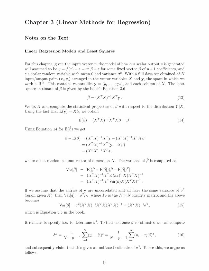
For this chapter, given the input vector x, the model of how our scalar output y is generatedwill assumed to be y = f(x) + ε = xTβ + ε for some fixed vector β of p+ 1 coefficients, andε a scalar random variable with mean 0 and variance σ2. With a full data set obtained of Ninput/output pairs (xi, yi) arranged in the vector variables X and y, the space in which wework is RN . This contains vectors like y = (y1, . . . , yN), and each column of X . The leastsquares estimate of β is given by the book’s Equation 3.6
β = (XTX)−1XTy . (13)
We fix X and compute the statistical properties of β with respect to the distribution Y |X .Using the fact that E(y) = Xβ, we obtain
E(β) = (XTX)−1XTXβ = β . (14)
Using Equation 14 for E(β) we get
β − E(β) = (XTX)−1XTy − (XTX)−1XTXβ
= (XTX)−1XT (y −Xβ)
= (XTX)−1XTε,
where ε is a random column vector of dimension N . The variance of β is computed as
Var[β] = E[(β − E[β])(β − E[β])T ]
= (XTX)−1XTE (εε)T X(XTX)−1
= (XTX)−1XTVar(ε)X(XTX)−1 .
If we assume that the entries of y are uncorrelated and all have the same variance of σ2
(again given X), then Var[ε] = σ2IN , where IN is the N ×N identity matrix and the abovebecomes
Var[β] = σ2(XTX)−1XTX(XTX)−1 = (XTX)−1σ2 , (15)
which is Equation 3.8 in the book.
It remains to specify how to determine σ2. To that end once β is estimated we can compute
σ2 =1
N − p− 1
N∑
i=1
(yi − yi)2 =
1
N − p− 1
N∑
i=1
(yi − xTi β)
2 , (16)
and subsequently claim that this gives an unbiased estimate of σ2. To see this, we argue asfollows.
14

Recall that we assume that each coordinate of the vector y is independent, and distributedas a normal random variable, centered at 0, with variance σ2. Since these N samples areindependent in the sense of probability, the probability measure of the vector y ∈ R
N is theproduct of these, denoted by N (0, σ2IN). This density has the following form
p(u) =1
(√2πσ
)N exp
(−u2
1 + . . .+ u2N
2σ2
),
where the ui are the coordinates of u and u ∈ RN . Now any orthonormal transformation of
RN preserves
∑Ni=1 u
2i . This means that the pdf is also invariant under any orthogonal trans-
formation keeping 0 fixed. Note that any function of u1, . . . , uk is probability independentof any function of uk+1, . . . , uN . Suppose that R
N = V ⊕W is an orthogonal decomposition,where V has dimension k and W has dimension N − k. Let v1, . . . , vk be coordinate func-tions associated to an orthonormal basis of V and let wk+1, . . . , wN be coordinate functionsassociated to an orthonormal basis of W . The invariance under orthogonal transformationsnow shows that the induced probability measure on V is N (0, σ2Ik). In particular the squareof the distance from 0 in V has distribution χ2
k. (However, this discussion does not appealto any properties of the χ2 distributions, so the previous sentence could have been omittedwithout disturbing the proof of Equation 3.8.)
If x is the standard variable in N (0, σ2), then E(x2) = σ2. It follows that the distancesquared from 0 in V ,
∑ki=1 v
2i , has expectation kσ2. We now use the fact that in ordinary
least squares y is the orthogonal projection of y onto the column space of X as a subspaceof RN . Under our assumption of the independence of the columns of X this later space hasdimension p+1. In the notation above y ∈ V with V the column space of X and y− y ∈ W ,where W is the orthogonal complement of the column space of X . Because y ∈ R
N and Vis of dimension p + 1, we know that W has dimension N − p − 1 and y − y is a randomvector in W with distribution N (0, σ2IN−p−1). The sum of squares of the N components
of y − y is the square of the distance in W to the origin. Therefore∑N
i=1 (yi − yi)2 has
expectation (N − p − 1)σ2. From Equation 16 we see that E(σ2) = σ2. This proves thebook’s Equation 3.8, which was stated in the book without proof.
Notes on the Prostate Cancer Example
In the R script duplicate table 3 1 N 2.R we provide explicit code that duplicates thenumerical results found in Table 3.1 and Table 3.2 using the above formulas for ordinaryleast squares. In addition, in that same function we then use the R function lm to verifythe same numeric values. Using the R package xtable we can display these correlations inTable 1. Next in Table 2 we present the results we obtained for the coefficients of the ordinaryleast squares fit. Notice that these coefficients are slightly different than the ones presentedin the book. These numerical values, generated from the formulas above, agree very closelywith the ones generated by the R command lm. I’m not sure where the discrepancy with thebook lies. Once this linear model is fit we can then apply it to the testing data and observehow well we do. When we do that we compute the expected squared prediction error (ESPE)
15

lcavol lweight age lbph svi lcp gleason pgg45lcavol 1.000 0.300 0.286 0.063 0.593 0.692 0.426 0.483
lweight 0.300 1.000 0.317 0.437 0.181 0.157 0.024 0.074age 0.286 0.317 1.000 0.287 0.129 0.173 0.366 0.276lbph 0.063 0.437 0.287 1.000 -0.139 -0.089 0.033 -0.030svi 0.593 0.181 0.129 -0.139 1.000 0.671 0.307 0.481lcp 0.692 0.157 0.173 -0.089 0.671 1.000 0.476 0.663
gleason 0.426 0.024 0.366 0.033 0.307 0.476 1.000 0.757pgg45 0.483 0.074 0.276 -0.030 0.481 0.663 0.757 1.000
Table 1: Duplication of the values from Table 3.1 from the book. These numbers exactlymatch those given in the book.
Term Coefficients Std Error Z Score1 (Intercept) 2.45 0.09 28.182 lcavol 0.72 0.13 5.373 lweight 0.29 0.11 2.754 age -0.14 0.10 -1.405 lbph 0.21 0.10 2.066 svi 0.31 0.13 2.477 lcp -0.29 0.15 -1.878 gleason -0.02 0.14 -0.159 pgg45 0.28 0.16 1.74
Table 2: Duplicated results for the books Table 3.2. These coefficients are slightly differentthan the ones presented in the book.
loss over the testing data points to be
ESPE ≈ 1
Ntest
Ntest∑
i=1
(yi − yi)2 = 0.521274 .
This value is relatively close the corresponding value presented in Table 3.3 of the book whichprovides a summary of many of the linear techniques presented in this chapter of 0.521. Tocompute the standard error of this estimate we use the formula
se(ESPE)2 =1
Ntest
Var(Y − Y) =1
Ntest
(1
Ntest − 1
Ntest∑
i=1
(yi − yi)2
).
This result expresses the idea that if the pointwise error has a variance of σ2 then the averageof Ntest such things (by the central limit theorem) has a variance given by σ2/Ntest. Usingthis we compute the standard error given by 0.1787240, which is relatively close from theresult presented in the book of 0.179.
16

Notes on the Gauss-Markov Theorem
Let θ be an estimator of the fixed, non-random parameter θ. So θ is a function of data.Since the data is (normally) random, θ is a random variable. We define the mean-square-error (MSE) of our estimator δ by
MSE(θ) := E((θ − θ)2
).
We can expand the quadratic (θ − θ)2 to get
(θ − θ)2 = (θ − E(θ) + E(θ)− θ)2
= (θ − E(θ))2 + 2(θ − E(θ))(E(θ)− θ) + (E(θ)− θ)2 .
Taking the expectation of this and remembering that θ is non random we have
MSE(θ − θ)2 = E(θ − θ)2
= Var(θ) + 2(E(θ)− E(θ))(E(θ)− θ) + (E(θ)− θ)2
= Var(θ) + (E(θ)− θ)2 , (17)
which is the book’s Equation 3.20.
At the end of this section the book shows that the expected quadratic error in the predictionunder the model f(·) can be broken down into two parts as
E(Y0 − f(x0))2 = σ2 +MSE(f(x0)) .
The first error component σ2 is unrelated to what model is used to describe our data. Itcannot be reduced for it exists in the true data generation process. The second source oferror corresponding to the term MSE(f(x0)) represents the error in the model and is undercontrol of the statistician (or the person doing the data modeling). Thus, based on the aboveexpression, if we minimize the MSE of our estimator f(x0) we are effectively minimizing theexpected (quadratic) prediction error which is our ultimate goal anyway. In this book wewill explore methods that minimize the mean square error. By using Equation 17 the meansquare error can be broken down into two terms: a model variance term and a model biassquared term. We will explore methods that seek to keep the total contribution of these twoterms as small as possible by explicitly considering the trade-offs that come from methodsthat might increase one of the terms while decreasing the other.
Multiple Regression from Simple Univariate Regression
As stated in the text we begin with a univariate regression model with no intercept i.e. noβ0 term as
Y = Xβ + ǫ .
The ordinary least square estimate of β are given by the normal equations or
β = (XTX)−1XTY .
17

Now since we are regressing a model with no intercept the matrix X is only a column matrixand the products XTX and XTY are scalars
(XTX)−1 = (N∑
i=1
x2i )
−1 and XTY =N∑
i=1
xiyi ,
so the least squares estimate of β is therefore given by
β =
∑Ni=1 xiyi∑Ni=1 x
2i
=xTy
xTx. (18)
Which is equation 3.24 in the book. The residuals ri of any model are defined in the standardway and for this model become ri = yi − xiβ.
When we attempt to take this example from p = 1 to higher dimensions, lets assume thatthe columns of our data matrix X are orthogonal that is we assume that 〈xT
j xk〉 = xTj xk = 0,
for all j 6= k then the outer product in the normal equations becomes quite simple
XTX =
xT1
xT2...xTp
[x1 x2 · · · xp
]
=
xT1 x1 xT
1 x2 · · · xT1 xp
xT2 x1 xT
2 x2 · · · xT2 xp
...... · · · ...
xTp x1 xT
p x2 · · · xTp xp
=
xT1 x1 0 · · · 00 xT
2 x2 · · · 0...
... · · · ...0 0 · · · xT
p xp
= D .
So using this, the estimate for β becomes
β = D−1(XTY ) = D−1
xT1 y
xT2 y...
xTp y
=
xT1 y
xT1 x1
xT2 y
xT2 x2
...xTp y
xTp xp
.
And each beta is obtained as in the univariate case (see Equation 18). Thus when the featurevectors are orthogonal they have no effect on each other.
Because orthogonal inputs xj have a variety of nice properties it will be advantageous to studyhow to obtain them. A method that indicates how they can be obtained can be demonstratedby considering regression onto a single intercept β0 and a single “slope” coefficient β1 thatis our model is of the given form
Y = β0 + β1X + ǫ .
When we compute the least squares solution for β0 and β1 we find (with some simple ma-nipulations)
β1 =n∑
xtyt − (∑
xt)(∑
yt)
n∑
x2t − (
∑xt)2
=
∑xtyt − x(
∑yt)∑
x2t − 1
n(∑
xt)2
=〈x− x1,y〉∑x2t − 1
n(∑
xt)2.
18

See [1] and the accompanying notes for this text where the above expression is explicitlyderived from first principles. Alternatively one can follow the steps above. We can write thedenominator of the above expression for β1 as 〈x− x1,x− x1〉. That this is true can be seenby expanding this expression
〈x− x1,x− x1〉 = xTx− x(xT1)− x(1Tx) + x2n
= xTx− nx2 − nx2 + nx2
= xTx− 1
n(∑
xt)2 .
Which in matrix notation is given by
β1 =〈x− x1,y〉
〈x− x1,x− x1〉 , (19)
or equation 3.26 in the book. Thus we see that obtaining an estimate of the second coefficientβ1 is really two one-dimensional regressions followed in succession. We first regress x onto1 and obtain the residual z = x − x1. We next regress y onto this residual z. The directextension of these ideas results in Algorithm 3.1: Regression by Successive Orthogonalizationor Gram-Schmidt for multiple regression.
Another way to view Algorithm 3.1 is to take our design matrix X , form an orthogonalbasis by performing the Gram-Schmidt orthogonilization procedure (learned in introductorylinear algebra classes) on its column vectors, and ending with an orthogonal basis zipi=1.Then using this basis linear regression can be done simply as in the univariate case by bycomputing the inner products of y with zp as
βp =〈zp,y〉〈zp, zp〉
, (20)
which is the books equation 3.28. Then with these coefficients we can compute predictionsat a given value of x by first computing the coefficient of x in terms of the basis zipi=1 (aszTp x) and then evaluating
f(x) =
p∑
i=0
βi(zTi x) .
From Equation 20 we can derive the variance of βp that is stated in the book. We find
Var(βp) = Var
(zTp y
〈zp, zp〉
)=
zTp Var(y)zp
〈zp, zp〉2=
zTp (σ2I)zp
〈zp, zp〉2
=σ2
〈zp, zp〉,
which is the books equation 3.29.
As stated earlier Algorithm 3.1 is known as the Gram-Schmidt procedure for multiple re-gression and it has a nice matrix representation that can be useful for deriving results thatdemonstrate the properties of linear regression. To demonstrate some of these, note that wecan write the Gram-Schmidt result in matrix form using the QR decomposition as
X = QR . (21)
19

In this decomposition Q is a N × (p + 1) matrix with orthonormal columns and R is a(p + 1)× (p+ 1) upper triangular matrix. In this representation the ordinary least squares(OLS) estimate for β can be written as
β = (XTX)−1XTy
= (RTQTQR)−1RTQTy
= (RTR)−1RTQTy
= R−1R−TRTQTy
= R−1QTy , (22)
which is the books equation 3.32. Using the above expression for β the fitted value y can bewritten as
y = Xβ = QRR−1QTy = QQTy , (23)
which is the books equation 3.33. This last equation expresses the fact in ordinary leastsquares we obtain our fitted vector y by first computing the coefficients of y in terms of thebasis spanned by the columns of Q (these coefficients are given by the vector QTy). We nextconstruct y using these numbers as the coefficients of the column vectors in Q (this is theproduct QQTy).
Notes on best-subset selection
While not applicable for larger problems it can be instructive to observe how best-subset se-lection could be done in practice for small problems. In the R script duplicate figure 3 5.R
we provide code that duplicates the numerical results found in Figure 3.5 from the book.The results from running this script are presented in Figure 1 . It should be noted that ingenerating this data we did not apply cross validation to selecting the value k that shouldbe used for the optimal sized subset to use for prediction accuracy. Cross validation of thistechnique is considered in a later section where 10 fold cross validation is used to estimatethe complexity parameter (k in this case) with the “one-standard-error” rule.
Notes on various linear prediction methods applied to the prostate data set
In this subsection we present numerical results that duplicate the linear predictive methodsdiscussed in the book. One thing to note about the implementation of methods is that manyof these methods “standardize” their predictors and/or subtract the mean from the responsebefore applying any subsequent techniques. Often this is just done once over the entireset of “training data” and then forgotten. For some of the methods and the subsequentresults presented here I choose do this scaling as part of the cross validation routine. Thus incomputing the cross validation (CV) errors I would keep the variables in their raw (unscaled)form, perform scaling on the training portion of the cross validation data, apply this scalingto the testing portion of the CV data and then run our algorithm on the scaled CV trainingdata. This should not result in a huge difference between the “scale and forget” method but
20

0 2 4 6 8
020
4060
8010
0
Subset Size k
Res
idua
l Sum
−of−
Squa
res
Figure 1: Duplication of the books Figure 3.5 using the code duplicate figure 3 5.R. Thisplot matches quite well qualitatively and quantitatively the corresponding one presented inthe book.
I wanted to mention this point in case anyone reads the provided code for the all subsetsand ridge regression methods.
In duplicating the all-subsets and ridge regression results in this section we wrote our own R
code to perform the given calculations. For ridge regression an alternative approach wouldhave been to use the R function lm.ridge found in the MASS package. In duplicating thelasso results in this section we use the R package glmnet [5], provided by the authors andlinked from the books web site. An interesting fact about the glmnet package is that forthe parameter settings α = 0 the elastic net penalization framework ignores the L1 (lasso)penalty on β and the formulation becomes equivalent to an L2 (ridge) penalty on β. Thisparameter setting would allow one to use the glmnet package to do ridge-regression if desired.Finally, for the remaining two regression methods: principal component regression (PCR)and partial least squares regression (PLSR) we have used the R package pls [7], which is apackage tailored to perform these two types of regressions.
As a guide to what R functions perform what coding to produce the above plots and table
21

Term LS Best Subset Ridge Lasso PCR PLS(Intercept) 2.452 2.452 2.452 2.452 2.452 2.452
lcavol 0.716 0.779 0.432 0.558 0.570 0.436lweight 0.293 0.352 0.252 0.183 0.323 0.360
age -0.143 -0.045 -0.153 -0.021lbph 0.212 0.168 0.216 0.243svi 0.310 0.235 0.088 0.322 0.259lcp -0.289 0.005 -0.050 0.085
gleason -0.021 0.042 0.228 0.006pgg45 0.277 0.134 -0.063 0.084
Test Error 0.521 0.492 0.492 0.484 0.448 0.536Std Error 0.178 0.143 0.161 0.166 0.104 0.149
Table 3: Duplicated results for the books Table 3.3. These coefficients are slightly differentthan the ones presented in the book but still show the representative ideas.
entries we have:
• The least squares (LS) results are obtained in the script duplicate table 3 1 N 2.R.
• The best subset results are obtained using the script dup OSE all subset.R.
• The ridge regression results are obtained using the script dup OSE ridge regression.R.
• The lasso results are obtained using the script dup OSE lasso.R.
• The PCR and PLS results are obtained using the script dup OSE PCR N PLSR.R.
We duplicate figure 3.7 from the book in Figure 2. We also duplicate table 3.3 from thebook in Table 3. There are some slight differences in the plots presented in Figure 2, seethe caption for that figure for some of the differences. There are also numerical differencesbetween the values presented in Table 3, but the general argument made in the book stillholds true. The idea that should be taken away is that all linear methods presented inthis chapter (with the exception of PLS) produce a linear model that outperforms the leastsquares model. This is important since it is a way for the applied statistician to make furtherimprovements in his application domain.
Notes on various shrinkage methods
After presenting ordinary least squares the book follows with a discussion on subset sectiontechniques: best-subset selection, forward- and backwards-stepwise selection, and forward-stagewise regression. The book’s concluding observation is that if it were possible best-subsetselection would be the optimal technique and should be used in every problem. The bookpresents two reasons (computational and statistical) why it is not possible to use best-subset
22

selection in many cases of practical interest. For most problems the computational reason isoverpowering since if we can’t even compute all of the subsets it will not be practical to usethis algorithm on applied problems. The difficulty with best-subset selection is that it is adiscrete procedure and there are too many required subsets to search over. The developmentof the various shrinkage method presented next attempt to overcome this combinatorialexplosion of best-subset by converting the discrete problem into a continuous one. Thecontinuous problems then turn out to be much simpler to solve. An example like this ofa technique we will study is ridge regression. Ridge regression constrains the sum of thesquares of the estimated coefficients βi (except for β0 which is dealt with separately) to beless than a threshold t. The effect of this constraint is to hopefully “zero out” the same βi
that would have been excluded by a best-subset selection procedure. If one wanted to mimicthe result of best-subset selection and truly wanted a fixed number, say M , of non-zerocoefficients βi, one could always simply zero the p−M smallest in magnitude βi coefficientsand then redo the ordinary least squares fit with the retained coefficients. In fact in Table 3.3we see that best-subset selection selected two predictors lcavol and lweight as predictors.If instead we had taken the ridge regression result and kept only the two features with thelargest values of |βi| we would have obtained the same two feature subset. While theseare certainly only heuristic arguments hopefully they will make understanding the followingmethods discussed below easier.
Notes on ridge regression
In this subsection of these notes we derive some of the results presented in the book. If wecompute the singular value decomposition (SVD) of the N × p centered data matrix X as
X = UDV T , (24)
where U is a N × p matrix with orthonormal columns that span the column space of X , Vis a p×p orthogonal matrix, and D is a p×p diagonal matrix with elements dj ordered suchthat d1 ≥ d2 ≥ · · · dp ≥ 0. From this representation of X we can derive a simple expressionfor XTX . We find that
XTX = V DUTUDV T = V D2V T . (25)
Using this expression we can compute the least squares fitted values yls = Xβ ls as
yls = Xβ ls = UDV T (V D2V T )−1V DUTy
= UDV T (V −TD−2V −1)V DUTy
= UUTy (26)
=
p∑
j=1
uj(uTj y) , (27)
where we have written this last equation in a form that we can directly compare to anexpression we will derive for ridge regression (specifically the books equation 3.47). Tocompare how the fitted values y obtained in ridge regression compare with ordinary leastsquares we next consider the SVD expression for βridge. In the same way as for least squares
23

we find
βridge = (XTX + λI)−1XTy (28)
= (V D2V T + λV V T )−1V DUTy
= (V (D2 + λI)V T )−1V DUTy
= V (D2 + λI)−1DUTy . (29)
Using this we can compute the product yridge = Xβridge. As in the above case for leastsquares we find
yridge = Xβridge = UD(D2 + λI)−1DUTy . (30)
Now note that in this last expression D(D2+λI)−1 is a diagonal matrix with elements given
byd2j
d2j+λand the vector UTy is the coordinates of the vector y in the basis spanned by the
p-columns of U . Thus writing the expression given by Equation 30 by summing columns weobtain
yridge = Xβridge =
p∑
j=1
uj
(d2j
d2j + λ
)uTj y . (31)
Note that this result is similar to that found in Equation 27 derived for ordinary least squares
regression but in ridge-regression the inner products uTj y are now scaled by the factors
d2jd2j+λ
.
Notes on the effective degrees of freedom df(λ)
The definition of the effective degrees of freedom df(λ) in ridge regression is given by
df(λ) = tr[X(XTX + λI)−1XT ] . (32)
Using the results in the SVD derivation of the expression Xβridge, namely Equation 30 butwithout the y factor, we find the eigenvector/eigenvalue decomposition of the matrix insidethe trace operation above given by
X(XTX + λI)−1XT = UD(D2 + λI)−1DUT .
From this expression the eigenvalues of X(XTX + λI)−1XT must be given by the elementsd2j
d2j+λ. Since the trace of a matrix can be shown to equal the sum of its eigenvalues we have
that
df(λ) = tr[X(XTX + λI)−1XT ]
= tr[UD(D2 + λI)−1DUT ]
=
p∑
j=1
d2jd2j + λ
, (33)
which is the books equation 3.50.
24

One important consequence of this expression is that we can use it to determine the valuesof λ for which to use when applying cross validation. For example, the book discusses howto obtain the estimate of y when using ridge regression and it is given by Equation 30 butno mention of the numerical values of λ we should use in this expression to guarantee thatwe have accurate coverage of all possible regularized linear models. The approach taken ingenerating the ridge regression results in Figures 2 and 8 is to consider df in Equation 33 afunction of λ. As such we set df(λ) = k for k = 1, 2, · · · , p representing all of the possiblevalues for the degree of freedom. We then use Newton’s root finding method to solve for λin the expression
p∑
i=1
d2jd2j + λ
= k .
To implement this root finding procedure recall that dj in the above expression are given bythe SVD of the data matrix X as expressed in Equation 24. Thus we define a function d(λ)given by
d(λ) =
p∑
i=1
d2jd2j + λ
− k , (34)
and we want λ such that d(λ) = 0. We use Newton’s algorithm for this where we iterategiven a starting value of λ0
λn+1 = λn −d(λn)
d′(λn).
Thus we need the derivative of d(λ) which is given by
d′(λ) = −p∑
i=1
d2j(d2j + λ)2
,
and an initial guess for λ0. Since we are really looking for p values of λ (one for each value ofk) we will start by solving the problems for k = p, p− 1, p− 2, · · · , 1. When k = p the valueof λ that solves df(λ) = p is seen to be λ = 0. For each subsequent value of k we use theestimate of λ found in the previous Newton solve as the initial guess for the current Newtonsolve. This procedure is implemented in the R code opt lambda ridge.R.
Notes on the lasso
When we run the code discussed on Page 20 for computing the lasso coefficients with theglmnet software we can also construct the profile of the βi coefficients as the value of λchanges. When we do this for the prostate data set we obtain Figure 4. This plot agreesquite well with the one presented in the book.
Notes on the three Bayes estimates: subset selection, ridge, and lasso
This would be a good spot for Davids discussion on the various reformulations of the con-strained minimization problem for β stating the two formulations and arguing their equiva-lence.
25

Below are just some notes scraped together over various emails discussing some facts that Ifelt were worth proving/discussing/understanding better:
λ is allowed to range over (0,∞) and all the solutions are different. But s is only allowed torange over an interval (0, something finite). If s is increased further the constrained solutionis equal to the unconstrained solution. That’s why I object to them saying there is a one-to-one correspondence. It’s really a one-to-one correspondence between the positive reals anda finite interval of positive numbers.
I’m assuming by s above you mean the same thing the book does s = t/∑p
1 |βj |q where q isthe ”power’ in the Lq regularization term. See the section 3.4.3 in the book) . Thus q = 1for lasso and q = 2 for ridge. So basically as the unconstrained solution is the least squaresone as then all estimated betas approach the least square betas. In that case the largestvalue for s is 1, so we actually know the value of the largest value of s. For values of s largerthan this we will obtain the least squares solution.
The one-to-one correspondence could be easily worked out by a computer program in anyspecific case. I don’t believe there is a nice formula.
Notes on Least Angle Regression (LAR)
To derive a better connection between Algorithm 3.2 (a few steps of Least Angle Regression)and the notation on the general LAR step “k” that is presented in this section that followsthis algorithm I found it helpful to perform the first few steps of this algorithm by hand andexplicitly writing out what each variable was. In this way we can move from the specificnotation to the more general expression.
• Standardize all predictors to have a zero mean and unit variance. Begin with allregression coefficients at zero i.e. β1 = β2 = · · · = βp = 0. The first residual will ber = y − y, since with all βj = 0 and standardized predictors the constant coefficientβ0 = y.
• Set k = 1 and begin start the k-th step. Since all values of βj are zero the first residualis r1 = y− y. Find the predictor xj that is most correlated with this residual r1. Thenas we begin this k = 1 step we have the active step given by A1 = xj and the activecoefficients given by βA1 = [0].
• Move βj from its initial value of 0 and in the direction
δ1 = (XTA1XA1)
−1XTA1r1 =
xTj r1
xTj xj
= xTj r1 .
Note that the term xTj xj in the denominator is not present since xT
j xj = 1 as allvariables are normalized to have unit variance. The path taken by the elements in βA1
can be parametrized by
βA1(α) ≡ βA1 + αδ1 = 0 + αxTj r1 = (xT
j r1)α for 0 ≤ α ≤ 1 .
26

This path of the coefficients βA1(α) will produce a path of fitted values given by
f1(α) = XA1βA1(α) = (xTj r1)αxj ,
and a residual of
r(α) = y − y − α(xTj r1)xj = r1 − α(xT
j r1)xj .
Now at this point xj itself has a correlation with this residual as α varies given by
xTj (r1 − α(xT
j r1)xj) = xTj r1 − α(xT
j r1) = (1− α)xTj r1 .
When α = 0 this is the maximum value of xTj r1 and when α = 1 this is the value 0.
All other features (like xk) have a correlation with this residual given by
xTk (r1 − α(xT
j r1)xj) = xTk r1 − α(xT
j r1)xTk xj .
Notes on degrees-of-freedom formula for LAR and the Lasso
From the books definition of the degrees-of-freedom of
df(y) =1
σ2
N∑
i=1
cov(yi, y) . (35)
We will derive the quoted expressions for df(y) under ordinary least squares regression andridge regression. We begin by evaluating cov(yi, y) under ordinary least squares. We firstrelate this scalar expression into a vector inner product expression as
cov(yi, yi) = cov(eTi y, eTi y) = eTi cov(y, y)ei .
Now for ordinary least squares regression we have y = Xβ ls = X(XTX)−1XTy, so that theabove expression for cov(y, y) becomes
cov(y, y) = X(XTX)−1XT cov(y, y) = σ2X(XTX)−1XT ,
since cov(y, y) = σ2I. Thus
cov(yi, yi) = σ2eTi X(XTX)−1XTei = σ2(XTei)(XTX)−1(XT ei) .
Note that the product XT ei = xi the ith samples feature vector for 1 ≤ i ≤ N and we havecov(yi, yi) = σ2xT
i (XTX)−1xi, which when we sum for i = 1 to N and divide by σ2 gives
df(y) =N∑
i=1
xTi (X
TX)−1xi
=
N∑
i=1
tr(xTi (X
TX)−1xi)
=N∑
i=1
tr(xixTi (X
TX)−1)
= tr
((N∑
i=1
xixTi
)(XTX)−1
).
27

Note that this sum above can be written as
N∑
i=1
xixTi =
[x1 x2 · · · xN
]
xT1
xT2...xTN
= XTX .
Thus when there are k predictors we get
df(y) = tr((XTX)(XTX)−1
)= tr(Ik×k) = k ,
the claimed result for ordinary least squares.
To do the same thing for ridge regression we can use Equation 28 to show
y = Xβridge = X(XTX + λI)−1XTy .
so thatcov(y, y) = X(XTX + λI)−1XT cov(y, y) = σ2X(XTX + λI)−1XT .
Again we can compute the scalar result
cov(yi, yi) = σ2(XT ei)T (XTX + λI)−1(XT ei) = σ2xT
i (XTX + λI)−1xi .
Then summing for i = 1, 2, · · · , N and dividing by σ2 to get
df(y) =
N∑
i=1
tr(xix
Ti (X
TX + λI)−1)
= tr(XTX(XTX + λI)−1
)
= tr(X(XTX + λI)−1XT
),
which is the books equation 3.50 providing an expression for the degrees of freedom for ridgeregression.
Methods Using Derived Input Directions: Principal Components Regression
Since the linear method of principal components regression (PCR) produced some of the bestresults (see Table 3) as far as the prostate data set it seemed useful to derive this algorithmin greater detail here in these notes. The discussion in the text is rather brief in this sectionwe bring the various pieces of the text together and present the complete algorithm in onelocation. In general PCR is parametrized by M for 0 ≤ M ≤ p (the number of principalcomponents to include). The values of M = 0 imply a prediction based on the mean of theresponse y and when M = p using PCR we duplicate the ordinary least squares solution (seeExercise 3.13 Page 41). The value of M used in an application is can be selected by crossvalidation (see Figure 2). One could imaging a computational algorithm such that given avalue of M would only compute the M principal components needed and no others. Sincemost general purpose eigenvector/eigenvalue code actually produces the entire eigensystemwhen supplied a given matrix the algorithm below computes all of the possible principalcomponent regressions (for 0 ≤ M ≤ p) in one step. The PCR algorithm is then given bythe following algorithmic steps:
28

• Standardize the predictor variables xi for i = 1, 2, . . . , p to have mean zero and varianceone. Demean the response y.
• Given the design matrix X compute the product XTX .
• Compute the eigendecomposition of XTX as
XTX = V D2V T .
The columns of V are denoted vm and the diagonal elements of D are denoted dm.
• Compute the vectors zm defined as zm = Xvm for m = 1, 2, . . . , p.
• Using these vectors zm compute the regression coefficients θm given by
θm =< zm, y >
< zm, zm >.
Note that we don’t need to explicitly compute the inner product < zm, zm > for eachm directly since using the eigendecomposition XTX = V D2V T computed above thisis equal to
zTmzm = vTmXTXvm = vTmV D2V Tvm = (V Tvm)
TD2(V Tvm) = eTmD2em = d2m ,
where em is a vector of all zeros with a one in the mth spot.
• Given a value of M for 0 ≤ M ≤ p, the values of θm, and zm the PCR estimate of y isgiven by
ypcr(M) = y1+
M∑
m=1
θmzm .
While the value of βpcr(M) which can be used for future predictions is given by
βpcr(M) =
M∑
m=1
θmvm .
This algorithm is implemented in the R function pcr wwx.R, and cross validation using thismethod is implemented in the function cv pcr wwx.R. A driver program that duplicates theresults from dup OSE PCR N PLSR.R is implemented in pcr wwx run.R. This version of thePCR algorithm was written to ease transformation from R to a more traditional programminglanguage like C++.
Note that the R package pcr [7] will implement this linear method and maybe more suitablefor general use since it allows input via R formula objects and has significantly more options.
29

Notes on Incremental Forward Stagewise Regression
Since the Lasso appears to be a strong linear method that is discussed quite heavily in thebook it would be nice to have some code to run that uses this method on a given problemof interest. There is the R package glmnet which solves a combined L2 and L1 constrainedminimization problem but if a person is programming in a language other than R you wouldhave to write your own L1 minimization routine. This later task is relatively complicated.Fortunately from the discussion in the text one can get the performance benefit of a lassotype algorithm but using a much simpler computational algorithm: Incremental ForwardStagewise Regression. To verify that we understood this algorithm we first implemented itin the R function IFSR.R. One interesting thing about this algorithm is that the version givenin the parametrized it based on ǫ, but provides no numerical details on how to specify thisvalue. In addition, once ǫ has been specified we need to develop an appropriate stoppingcriterion. The book suggested to run the code until the residuals are uncorrelated withall of the predictors. In the version originally implemented the algorithm was allowed toloop until the largest correlation between the residual r and each feature xj is smaller thana given threshold. One then has to pick the value of this threshold. Initially the value Iselected was too large in that the p value cor(xj , r) never got small enough. I then addeda maximum number of iterations to perform where in each iteration we step an amount ǫin the j component of β. Again one needs to now specify a step size ǫ and a maximumnumber of iterations Nmax. If ǫ is taken very small then one will need to increase the valueof Nmax. If ǫ is taken large one will need to decrease Nmax. While not difficult to modifythese parameters and look at the profile plots of β for a single example it seemed useful tohave a nice way of automatically determining ǫ given an value of Ntest. To do that I foundthat the simple heuristic of
ǫ =||βLS||11.5Nmax
. (36)
gives a nice way to specify ǫ in terms of Nmax. Here ||βLS||1 is the one norm of the leastsquares solution for β given by Equation 13. The motivation for this expression is thatthis algorithm starts at the value β = 0 and takes “steps” of “size” ǫ towards βLS. If we
want a maximum of Nmax steps then we should take ǫ of size ||βLS||1Nmax
so that we get thereat the last step. The factor of 1.5 is to make the values of ǫ we use for stepping somewhatsmaller. Another nice benefit of this approach is that the amount of computation for thisalgorithm then scales as O(Nmax) so depending on problem size one can pick a value of Nmax
that is reasonable as far as the required computational time. It is then easy to estimatethe computational time if this algorithm was run with 2Nmax. It seems more difficult to dothat if the value of ǫ is given a priori and instead we are asked estimate the time to run thealgorithm with ǫ
2.
30
Exercise Solutions
Ex. 3.1 (the F -statistic is equivalent to the square of the Z-score)
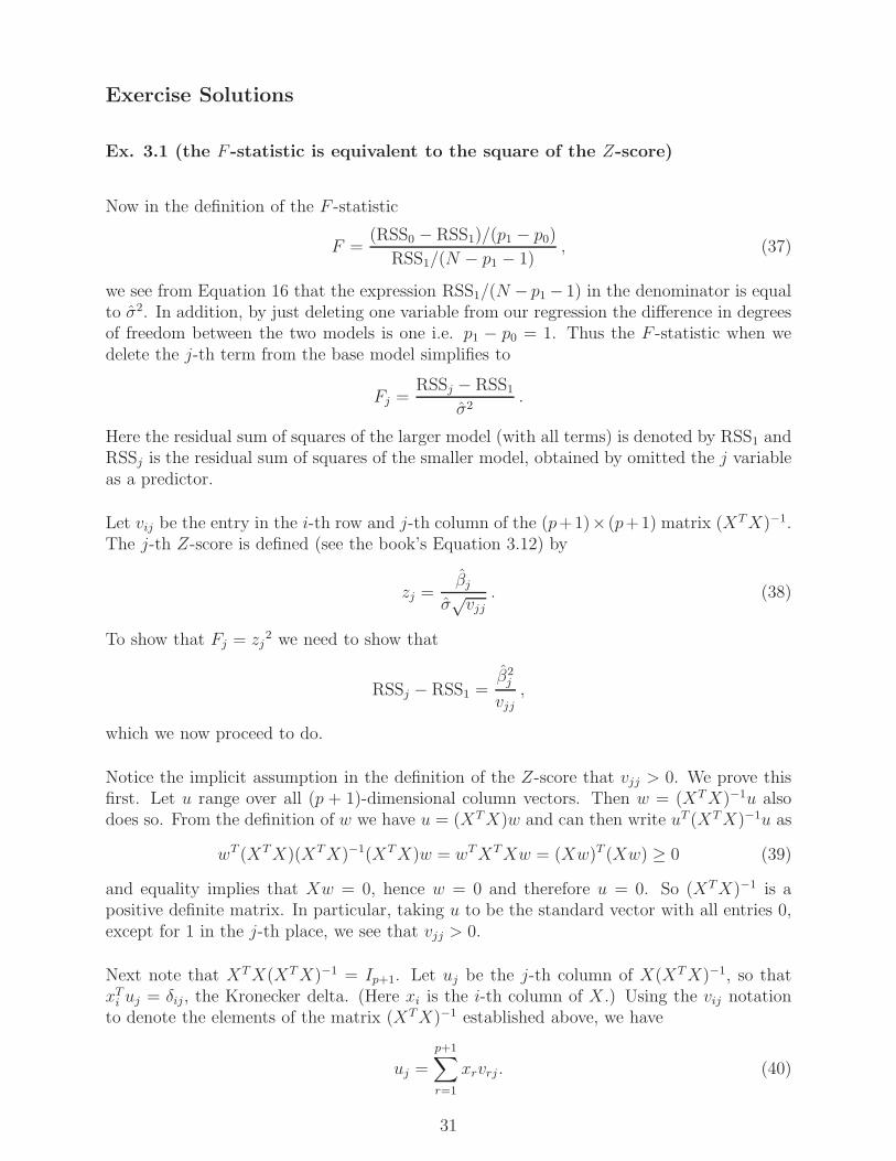
Now in the definition of the F -statistic
F =(RSS0 − RSS1)/(p1 − p0)
RSS1/(N − p1 − 1), (37)
we see from Equation 16 that the expression RSS1/(N − p1 − 1) in the denominator is equalto σ2. In addition, by just deleting one variable from our regression the difference in degreesof freedom between the two models is one i.e. p1 − p0 = 1. Thus the F -statistic when wedelete the j-th term from the base model simplifies to
Fj =RSSj − RSS1
σ2.
Here the residual sum of squares of the larger model (with all terms) is denoted by RSS1 andRSSj is the residual sum of squares of the smaller model, obtained by omitted the j variableas a predictor.
Let vij be the entry in the i-th row and j-th column of the (p+1)× (p+1) matrix (XTX)−1.The j-th Z-score is defined (see the book’s Equation 3.12) by
zj =βj
σ√vjj
. (38)
To show that Fj = zj2 we need to show that
RSSj − RSS1 =β2j
vjj,
which we now proceed to do.
Notice the implicit assumption in the definition of the Z-score that vjj > 0. We prove thisfirst. Let u range over all (p + 1)-dimensional column vectors. Then w = (XTX)−1u alsodoes so. From the definition of w we have u = (XTX)w and can then write uT (XTX)−1u as
wT (XTX)(XTX)−1(XTX)w = wTXTXw = (Xw)T (Xw) ≥ 0 (39)
and equality implies that Xw = 0, hence w = 0 and therefore u = 0. So (XTX)−1 is apositive definite matrix. In particular, taking u to be the standard vector with all entries 0,except for 1 in the j-th place, we see that vjj > 0.
Next note that XTX(XTX)−1 = Ip+1. Let uj be the j-th column of X(XTX)−1, so thatxTi uj = δij, the Kronecker delta. (Here xi is the i-th column of X .) Using the vij notation
to denote the elements of the matrix (XTX)−1 established above, we have
uj =
p+1∑
r=1
xrvrj . (40)
31

We have seen that, for i 6= j, uj/vjj is orthogonal to xi, and the coefficient of xj in uj/vjj is1. Permuting the columns of X so that the j-th column comes last, we see that uj/vjj = zj(see Algorithm 3.1). By Equation 40,
‖uj‖2 = uTj uj =
p+1∑
r=1
vrjxTr uj =
p+1∑
r=1
vrjδrj = vjj.
Then
‖zj‖2 =‖uj‖2v2jj
= vjj/v2jj =
1
vjj. (41)
Now zj/‖zj‖ is a unit vector orthogonal to x1, . . . , xj−1, xj+1, . . . , xp+1. So
RSSj − RSS1 = 〈y, zj/‖zj‖〉2
=
( 〈y, zj〉〈zj, zj〉
)2
‖zj‖2
= β2j /vjj,
where the final equality follows from Equation 41 and the book’s Equation 3.28.
Ex. 3.2 (confidence intervals on a cubic equation)
In this exercise, we fix a value for the column vector β = (β0, β1, β2, β3)T and examine
random deviations from the curve
y = β0 + β1x+ β2x2 + β3x
3.
For a given value of x, the value of y is randomized by adding a normally distributed variablewith mean 0 and variance 1. For each x, we have a row vector x = (1, x, x2, x3). We fix Nvalues of x. (In Figure 6 we have taken 40 values, evenly spaced over the chosen domain[−2, 2].) We arrange the corresponding values of x in an N × 4-matrix, which we call X , asin the text. Also we denote by y the corresponding N × 1 column vector, with independent
entries. The standard least squares estimate of β is given by β =(XTX
)−1XTy. We now
compute a 95% confidence region around this cubic in two different ways.
In the first method, we find, for each x, a 95% confidence interval for the one-dimensionalrandom variable u = x.β. Now y is a normally distributed random variable, and thereforeso is β = (XTX)−1XTy. Therefore, using the linearity of E,
Var(u) = E(xββTxT
)− E
(xβ).E(βTxT
)= xVar(β)xT = x
(XTX
)−1xT .
This is the variance of a normally distributed one-dimensional variable, centered at x.β, andthe 95% confidence interval can be calculated as usual as 1.96 times the square root of thevariance.
32

In the second method, β is a 4-dimensional normally distributed variable, centered at β, with
4× 4 variance matrix(XTX
)−1. We need to take a 95% confidence region in 4-dimensional
space. We will sample points β from the boundary of this confidence region, and, for eachsuch sample, we draw the corresponding cubic in green in Figure 6 on page 59. To see whatto do, take the Cholesky decomposition UTU = XTX , where U is upper triangular. Then(UT )−1
(XTX
)U−1 = I4, where I4 is the 4×4-identity matrix. Uβ is a normally distributed
4-dimensional variable, centered at Uβ, with variance matrix
Var(Uβ) = E(UββTUT
)− E
(Uβ).E(βTUT
)= U
(XTX
)−1UT = I4
It is convenient to define the random variable γ = β − β ∈ R4, so that Uγ is a standard
normally distributed 4-dimensional variable, centered at 0.
Using the R function qchisq, we find r2, such that the ball B centered at 0 in R4 of radius
r has χ24-mass equal to 0.95, and let ∂B be the boundary of this ball. Now Uγ ∈ ∂B if and
only if its euclidean length squared is equal to r2. This means
r2 = ‖Uγ‖2 = γTUTUγ = γTXTXβ.
Given an arbitrary point α ∈ R4, we obtain β in the boundary of the confidence region by
first dividing by the square root of γTXTXγ and then adding the result to β.
Note that the Cholesky decomposition was used only for the theory, not for the purposes ofcalculation. The theory could equally well have been proved using the fact that every realpositive definite matrix has a real positive definite square root.
Our results for one particular value of β are shown in Figure 6 on page 59.
Ex. 3.3 (the Gauss-Markov theorem)
(a) Let b be a column vector of length N , and let E(bT y) = αTβ. Here b is fixed, and theequality is supposed true for all values of β. A further assumption is that X is not random.Since E(bT y) = bTXβ, we have bTX = αT . We have
Var(αT β) = αT (XTX)−1α = bTX(XTX)−1XT b,
and Var(bT y) = bT b. So we need to prove X(XTX)−1XT IN .
To see this, write X = QR where Q has orthonormal columns and is N × p, and R is p× pupper triangular with strictly positive entries on the diagonal. Then XTX = RTQTQR =RTR. Therefore X(XTX)−1XT = QR(RTR)−1RTQT = QQT . Let [QQ1] be an orthogonalN ×N matrix. Therefore
IN =[Q Q1
].
[QT
QT1
]= QQT +Q1Q
T1 .
Since Q1QT1 is positive semidefinite, the result follows.
33

(b) Let C be a constant p × N matrix, and let Cy be an estimator of β. We write C =(XTX)−1XT + D. Then E(Cy) =
((XTX)−1XT +D
)Xβ. This is equal to β for all β if
and only if DX = 0. We have Var(Cy) = CCTσ2, Using DX = 0 and XTDT = 0, we find
CCT =((XTX)−1XT +D
) ((XTX)−1XT +D
)T
= (XTX)−1 +DDT
= Var(β)σ−2 +DDT .
The result follows since DDT is a positive semidefinite p× p-matrix.
(a) again. Here is another approach to (a) that follows (b), the proof for matrices. Let c be alength N row vector and let cy be an estimator of αTβ. We write c = αT
((XTX)−1XT
)+d.
Then E(cy) = αTβ + dXβ. This is equal to αTβ for all β if and only if dX = 0. We haveVar(cy) = ccTσ2, Using dX = 0 and XTdT = 0, we find
ccT =(αT((XTX)−1XT
)+ d).(αT((XTX)−1XT
)+ d)T
= αT (XTX)−1α+ ddT
The result follows since ddT is a non-negative number.
Ex. 3.4 (the vector of least squares coefficients from Gram-Schmidt)
The values of βi can be computed by using Equation 22, where Q and R are computed fromthe Gram-Schmidt procedure on X . As we compute the columns of the matrix Q in theGram-Schmidt procedure we can evaluate qTj y for each column qj of Q, and fill in the jthelement of the vector QTy. After the matrices Q and R are computed one can then solve
Rβ = QTy . (42)
for β to derive the entire set of coefficients. This is simple to do since R is upper triangularand is performed with back-substitution, first solving for βp+1, then βp, then βp−1, and on
until β0. A componentwise version of backwards substitution is presented in almost everylinear algebra text.
Note: I don’t see a way to compute βi at the same time as one is computing the columns ofQ. That is, as one pass of the Gram-Schmidt algorithm. It seems one needs to othogonalizeX first then solve Equation 42 for β.
Ex. 3.5 (an equivalent problem to ridge regression)
Consider that the ridge expression problem can be written as (by inserting zero as xj − xj)
N∑
i=1
(yi − β0 −
p∑
j=1
xjβj −p∑
j=1
(xij − xj)βj
)2
+ λ
p∑
j=1
β2j . (43)
34

From this we see that by defining “centered” values of β as
βc0 = β0 +
p∑
j=1
xjβj
βcj = βi i = 1, 2, . . . , p ,
that the above can be recast as
N∑
i=1
(yi − βc
0 −p∑
j=1
(xij − xj)βcj
)2
+ λ
p∑
j=1
βcj2
The equivalence of the minimization results from the fact that if βi minimize its respectivefunctional the βc
i ’s will do the same.
A heuristic understanding of this procedure can be obtained by recognizing that by shiftingthe xi’s to have zero mean we have translated all points to the origin. As such only the“intercept” of the data or β0 is modified the “slope’s” or βc
j for i = 1, 2, . . . , p are notmodified.
We compute the value of βc0 in the above expression by setting the derivative with respect
to this variable equal to zero (a consequence of the expression being at a minimum). Weobtain
N∑
i=1
(yi − βc
0 −p∑
j=1
(xij − xj) βj
)= 0,
which implies βc0 = y, the average of the yi. The same argument above can be used to
show that the minimization required for the lasso can be written in the same way (with βcj2
replaced by |βcj |). The intercept in the centered case continues to be y.
Ex. 3.6 (the ridge regression estimate)
Note: I used the notion in original problem in [6] that has τ 2 rather than τ as the varianceof the prior. Now from Bayes’ rule we have
p(β|D) ∝ p(D|β)p(β) (44)
= N (y −Xβ, σ2I)N (0, τ 2I) (45)
Now from this expression we calculate
log(p(β|D)) = log(p(D|β)) + log(p(β)) (46)
= C − 1
2
(y −Xβ)T (y −Xβ)
σ2− 1
2
βTβ
τ 2(47)
here the constant C is independent of β. The mode and the mean of this distribution (withrespect to β) is the argument that maximizes this expression and is given by
β = ArgMin(−2σ2 log(p(β|D)) = ArgMin((y −Xβ)T (y −Xβ) +σ2
τ 2βTβ) (48)
35

Since this is the equivalent to Equation 3.43 page 60 in [6] with the substitution λ = σ2
τ2we
have the requested equivalence.
Exs3.6 and 3.7 These two questions are almost the same; unfortunately they are bothsomewhat wrong, and in more than one way. This also means that the second-last paragraphon page 64 and the second paragraph on page 611 are both wrong. The main problem is thatβ0 is does not appear in the penalty term of the ridge expression, but it does appear in theprior for β. . In Exercise 3.6, β has variance denoted by τ , whereas the variance is denotedby τ 2 in Exercise 3.7. We will use τ 2 throughout, which is also the usage on page 64.
With X = (x1, . . . , xp) fixed, Bayes’ Law states that p(y|β).p(β) = p(β|y).p(y). So, theposterior probability satisfies
p(β|y) ∝ p(y|β).p(β),where p denotes the pdf and where the constant of proportionality does not involve β. Wehave
p(β) = C1 exp
(−‖β‖2
2τ 2
)
and
p(y|β) = C2 exp
(−‖y −Xβ‖2
2σ2
)
for appropriate constants C1 and C2. It follows that, for a suitable constant C3,
p(β|y) = C3 exp
(−‖y −Xβ‖2 + (σ2/τ 2).‖β‖2
2σ2
)(49)
defines a distribution for β given y, which is in fact a normal distribution, though notcentered at 0 and with different variances in different directions.
We look at the special case where p = 0, in which case the penalty term disappears andridge regression is identical with ordinary linear regression. We further simplify by takingN = 1, and σ = τ = 1. The ridge estimate for β0 is then
argminβ
(β0 − y1)
2= y1.
The posterior pdf is given by
p(β0|y1) = C4 exp
(−(y1 − β0)
2 + β20
2
)= C5 exp
(−(β0 −
y12
)2),
which has mean, mode and median equal to y1/2, NOT the same as the ridge estimatey1. Since the integral of the pdf with respect to β0(for fixed y1) is equal to 1, we see thatC5 = 1/
√2π. Therefore the log-posterior is equal to
− log(2π)/2 +(β0 −
y12
)= − log(2π)/2 + (β0 − y1)
2
To retrieve a reasonable connection between ridge regression and the log-posterior, we needto restrict to problems where β0 = 0. In that case, the claim of Exercise 3.6 that the ridgeestimate is equal to the mean (or the mode) of the posterior distribution becomes true.
36

We set λ = σ2/τ 2. From Equation 49 on page 36 for the posterior distribution of β, we findthat the minus log-posterior is not proportional to
N∑
i=1
(yi −
p∑
j=1
xijβj
)2
+ λ
p∑
j=1
β2j
as claimed, because the term log(C3) has been omitted.
Ex. 3.8 (when is the QR decomposition equivalent to the SV D decomposition)
This exercise is true if X has rank p + 1, and is false otherwise. Let X = QR, whereQ = (q0, . . . , qp) is N × (p + 1) with orthonormal columns, and R is upper triangular withstrictly positive diagonal entries. We write the entries of R as rkj in the k-th row and j-thcolumn, where 0 ≤ k, j ≤ p. Let e be the length N column matrix consisting entirely ofones. Then e = r00q0. We deduce that all the entries of q0 are equal. Since ‖q0‖ = 1 andr00 > 0, we see that q0 = e/
√N and that r00 =
√N . The columns of Q form a basis for the
column-space of X . Therefore the columns of Q2 form a basis for the orthogonal complementof e in the column-space of X . For 1 ≤ j ≤ p, we have
qj =
N∑
i=1
qij/N = eT .qj/N = qT0 .qj/√N = 0.
Let X = (e, x1, . . . , xp) = QR. Then xj =∑j
k=0 rkjqk, and so xj = r0j/√N . We have
xje = r0jq0, and so xj − xje =
p∑
k=1
rkjqk. (50)
Let R2 be the lower right p× p submatrix of R. Then
R =
(√N
√N(x1, . . . , xp)
0 R2
).
Using Equation 50 above, we have
Q2R2 = X = UDV T . (51)
Since X is assumed to have rank p+ 1, DV T is a non-singular p× p matrix. It follows thatU , X and Q2 have the same column space.
We assume that, by “up to sign flips”, the authors mean that the columns (as opposed tothe rows) of Q2 and U are the same, up to sign. In this case, multiplying Equation 51 byQT
2 , we see that R2 = D1DV T , where D1 is a diagonal matrix with entries ±1. Since V is anorthogonal matrix, R2 has orthogonal rows. Also R2 has strictly positive diagonal entries. It
37

follows that R2 is a diagonal matrix, and so the columns of X are orthogonal to each other.Therefore V is also diagonal, and the entries must all be ±1.
Now let’s look at the converse, where we suppose that X has orthogonal columns. Sincethe QR decomposition is unique (see ???), we see that the QR decomposition of X = Q2R2,where R2 is diagonal with strictly positive entries. This is also an SVD, with U = Q2 andV = Ip. However, it is not true that U = Q2 for every SVD. Suppose, for example X = Inis the identity matrix. Then Q2 = R2 = In, and we can take U = V to be any orthogonalmatrix of the right size.
Ex. 3.9 (using the QR decomposition for fast forward-stepwise selection)
If we fit an ordinary least squares linear model with q terms then the QR decompositionof X1 or the equation X1 = QR and Equation 23 expresses y as a sum of q columns of Q.Thus y is the span of the columns of Q. Since Q is related to X1 by the Gram-Schmidtorthogonilization process y is also in the span of the q columns of X1. By properties of leastsquare estimates the residual r = y − y is in the orthogonal complement of the columns ofboth Q and X1. To pick the next column xj of the p − q possible choices to add next, theone we should pick should be the column that had the largest projection in the direction ofr. Thus we want to pick xj that is most parallel with r to add next. Thus pick j∗ such that
j∗ = argminj
|xTj r|
||xj||,
This xj will reduce the residual sum of squares the most.
Note: I don’t see explicitly why we need the QR algorithm in this expression.
Let X1 = QR be the QR decomposition, and let zi be the i-th column of Q (1 ≤ i ≤ q). SoQTQ = Iq and R is upper triangular with strictly positive diagonal entries. The collectionz1, . . . , zq is an orthonormal basis of C0, the column space of X1. C0 is also the columnspace of Q. Let y be the orthogonal projection of the N -dimensional vector y to C0.
For each j (q < j ≤ p), let Cj be the subspace of RN spanned by C0 and xj , the (j − q)-thcolumn of X2. We define
uj = xj −q∑
i=1
(zTi xj)zi and (52)
vj = uj/‖uj‖ (53)
and so z1, . . . , zq, vj is an orthonormal basis of Cj. Now yj = y+(vTj y)vj is the orthogonalprojection of y to Cj, and so the residual sum of squares decreases by (vTj y)
2 if y is replaced
by yj. It follows that the best variable to include is the k-th, where k = argmaxq<j≤p
∣∣vTj y∣∣.
We then set zq+1 = vk.
Note that, during the computation, we need to know zTi xj for all i and j (1 ≤ i ≤ qand q < j ≤ p. We have therefore done already completed of the computation necessary
38

to include yet another variable in our Stepwise Forward Linear Regression. So this seemsreasonably efficient, and we know of no more efficient algorithm (but there may be a moreefficient algorithm that we don’t know about).
Ex. 3.10 (using the z-scores for fast backwards stepwise regression)
The F -statistic
F =(RSS0 − RSS1)/(p1 − p0)
RSS1/(N − p1 − 1),
when we drop a single term from the larger model (with residual sum of squares given byRSS1) we will have p1 − p0 = 1, since the change in the degrees of freedom between thetwo models is only one. In this case when we drop the j-th term from the regression theF -statistic simplifies slightly and becomes
Fj =RSSj − RSS1
RSS1/(N − p1 − 1).
This is a scaled version (scaled by the division of the expression RSS1/(N − p1 − 1)) ofthe increase in the residual sum of squares we observe when we drop the j-th term. FromExercise 3.1 this expression is equal to z2j the square of the j-th z-score
zj =βj
σ√vj
.
Thus by picking the index j∗ that is associated with the smallest z-score and then deletingthat variable from our regression we will be selecting the variable xj∗ that when deleted fromthe model will increase the residual sum of squares the least.
Ex. 3.11 (multivariate linear regression with different Σi)
The question refers to the book’s Equations 3.39 and 3.40. To recall the notation, thefollowing variables refer to matrices of the given sizes: Y size N ×K, X size N × (p+ 1),B size (p+ 1)×K. Equation 3.38 gives the sum of squares as
RSS(B) = tr[(Y −XB)(Y −XB)T
].
In the book, the two factors are written in the other order. We are using the fact thattr(UV ) = tr(V U) for any matrices U and V , provided both products make sense.
To prove Equation 3.39, we equate to zero the derivative of RSS(B) with respect to B.Using the fact that the trace of a square matrix is equal to the trace of its transpose, we seethat this condition on the derivative is equivalent to the condition that, for all (p + 1)×Kmatrices A, we have
tr((XA)T (Y −XB)) = 0.
39

Let A be equal to zero, except for a 1 in row j and column k. The condition becomes∑i xij (yik −
∑s xisbsk) = 0, for each j and k. But this is the condition XT (Y −XB) = 0.
Multiplying on the left by the inverse of XTX, we obtain Equation 3.39.
In order to deal with the situation of Equation 3.40, we rewrite it as
RSS(B,Σ) = tr[(Y −XB)Σ−1(Y −XB)T
].
As a positive definite symmetric matrix, Σ−1 has a positive definite symmetric square root,which we denote by S, a K × K matrix. We replace Y by YS and B by BS. Thisreduces us to the previous case, which, by Equation 3.39, gives a minimum value whenBS = (XTX)−1XTYS, and we multiply on the right by S−1 to obtain the usual formula(Equation 3.39) for B.
Now suppose that the correlations Σi vary from one sample to the next. We will not gointo the question of how to estimate these correlations, which seems to be possible onlyunder some additional assumptions. Instead we assume that these correlations are known.Then there is no closed formula like Equation 3.39 for B. However the corresponding sumof squares is, in general, a positive definite quadratic form whose variables are the entries ofB. The argmin is therefore easy to find, using the specific values of X, Y. This can be doneeither with a computer program or analytically by diagonalizing the quadratic form.
Ex. 3.12 (ordinary least squares to implement ridge regression)
Consider the input centered data matrix X (of size pxp) and the output data vector Y bothappended (to produce the new variables X and Y ) as follows
X =
[X√λIpxp
](54)
and
Y =
[Y
Opx1
](55)
with Ipxp and Opxp the pxp identity and px1 zero column respectively. The the classic leastsquares solution to this new problem is given by
βLS = (XT X)−1XT Y (56)
Performing the block matrix multiplications required by this expression we see that
XT X =[XT
√λIpxp
] [ X√λIpxp
]= XTX + λIpxp (57)
and
XT Y =[XT
√λ] [ Y
Opx1
]= XTY (58)
Thus equation 56 becomesβLS = (XTX + λIpxp)
−1XTY (59)
40

This expression we recognize as the solution to the regularized least squares proving theequivalence.
In a slightly different direction, but perhaps related, I was thinking of sending an email tothe authors with some comments on some of the questions. For example, I think 3.7 (online)is incorrect, as there should be an additive constant as well as a multiplicative constant.The question is of course almost the same as 3.6, except for the spurious change from τto τ 2. There are sometimes questions that involve some mind-reading by the reader. Forexample, I don’t like the word ”characterize” in 3.5. According to the dictionary, this means”describe the distinctive character of”. Mind-reading is required. Another bugbear is theword ”Establish” in the online Exercise 2.7(d). And there aren’t two cases, there are at leastfour (nearest neighbour, linear, unconditional, conditional on keeping X fixed, more if k isallowed to vary.) And do they mean a relationship between a squared bias and variance ineach of these four cases?
Ex. 3.13 (principal component regression)
Recall that principal component regression (PCR) using M components, estimates coeffi-cients θm, based on the top M largest variance principal component vectors zm. As such ithas a expression given by
ypcr(M) = y1 +
M∑
m=1
θmzm (60)
= y1 +XM∑
m=1
θmvm ,
using the fact that zm = Xvm and writing the fitted value under PCR as a function of thenumber of retained components M . The above can be written in matrix form involving thedata matrix as
ypcr(M) =[1 X
] [ y∑Mm=1 θmvm
].
We can write this as the matrix[1 X
]times a vector βpcr if we take this later vector as
βpcr(M) =
[y∑M
m=1 θmvm
]. (61)
This is the same as the books equation 3.62 when we restrict to just the last p elements ofβpcr. It can be shown (for example in [10]) that for multiple linear regression models theestimated regression coefficients in the vector β can be split into two parts a scalar β0 anda p× 1 vector β∗ as
β =
[β0
β∗
].
In addition the coefficient β0 can be shown to be related to β∗ as
β0 = y − β∗x ,
41

where y is the scalar mean of the response vector y and x is the p × 1 vector where eachcomponent hold the mean of a predictor say xi. Since from Equation 61 we see that β0 = yand can conclude that in principal component regression x = 0 or that the input predictorvariables are standardized.
To evaluate βpcr(M) when M = p recall that in principal component regression the vectorsvm are from the SVD of the matrix X given by X = UDV T . This later expression isequivalent to XV = UD from which if we equate the columns of the matrices on both sideswe get
Xv1 = d1u1
Xv2 = d2u2
...
Xvp = dpup .
Since the vectors zm are given by zm = Xvm for 1 ≤ m ≤ M ≤ p, by the above we have thevectors zm in terms of the vectors um as zm = dmum. Since for this problem we are to showthat when M = p the estimate βpcr(M) above becomes the least squares estimate β ls it ishelpful to see what this later estimate looks like interms of the SVD matrices U , D, and V .Recognizing that when λ = 0 the ridge regression estimate for β is equal to the least squaresestimate (when λ = 0 we have no λ||β||22 ridge penalty term) we can use Equation 29 toobtain
β ls = βridge(λ = 0) = V D−2DUT y = V D−1UTy . (62)
We now see if we can transform βpcr(p) into this expression. We have
βpcr(p) =
p∑
m=1
θmvm = V
θ1θ2...
θp
= V
<z1,y><z1,z1><z2,y><z2,z2>
...<zp,y><zp,zp>
.
Using zm = dmum derived above we have
< zm, zm >= d2m < um, um >= d2m ,
since the vectors um are assumed to be orthonormal. Also < zm, y >= dm < um, y >, so theestimate for βpcr(p) becomes
βpcr(p) = V
<u1,y>d1
<u2,y>d2...
<up,y>dp
= V D−1UT y ,
which by Equation 62 equals β ls as we were to show.
42

Ex. 3.14 (when the inputs are orthogonal PLS stops after m = 1 step)
Observe that in Algorithm 3.3 on partial least squares (PLS) if on any given step m wecompute that φmj = 0 for all j then it follows that the algorithm must stop. For thisproblem when the xj ’s are orthonormal we will explicitly walk through the first step of the
algorithm by hand and show that φ2j = 0 for all 1 ≤ j ≤ p.
Note that the xj ’s to be orthogonal means that xTi xj = 0 for all i 6= j. Following each step
of Algorithm 3.3 and starting with m = 1 we have
(a) We have that z1 is given by
z1 =
p∑
j=1
φ1jx(0)j with φ1j =< x
(0)j , y > .
(b) Next we compute θ1 =<z1,y><z1,z1>
. The denominator in the above fraction is given by
< z1, z1 > = 〈p∑
j=1
φ1jx(0)j ,
p∑
j=1
φ1jx(0)j 〉 =
p∑
j=1
p∑
j′=1
φ1jφ1j′〈x(0)j , x
(0)j′ 〉
=
p∑
j=1
p∑
j′=1
φ1jφ1j′δjj′ =
p∑
j=1
φ21j ,
since the vectors x(0)j are orthogonal. The numerator in the above expression for θ1 is
given by
< z1, y >=
p∑
j=1
φ1j < x(0)j , y >=
p∑
j=1
φ21j ,
and thus we have θ1 = 1.
(c) Next we find y(1) given by
y(1) = y(0) + z1 = y(0) +
p∑
j=1
φ1jx(0)j .
(d) Next we compute x(1)j for each value of j = 1, 2, . . . , p using
x(1)j = x
(0)j − < z1, x
(0)j >
< z1, z1 >z1 .
Since the vectors x(0)j are orthogonal the inner product in the numerator above becomes
< z1, x(0)k >=
p∑
j=1
φ1j < x(0)j , x
(0)k >= φ1k .
43

Using this result x(1)j becomes
x(1)j = x
(0)j − φ1j∑p
j=1 φ21j
z1
= x(0)j −
(φ1j∑pj=1 φ
21j
)p∑
j=1
φ1jx(0)j .
Having finished the first loop of Algorithm 3.3 we let m = 2 and compute φ2j to get
φ2j = < x(1)j , y >=< x
(0)j , y > −
(φ1j∑pj=1 φ
21j
)p∑
j=1
φ21j
= 0 .
Thus as discussed at the beginning of this problem since φ2j = 0 the algorithm must stop.
Ex. 3.15 (PLS seeks directions that have high variance and high correlation)
This problem has not yet been worked.
Ex. 3.16 (explicit expressions for βj when the features are orthonormal)
When the predictors are orthonormal XTX = I and the ordinary least squared estimate ofβ is given by
β = XTY . (63)
In best-subset selection we will take the top M predictors that result in the smallest residualsum of squares. Since the columns of X are orthonormal we can construct a basis for R
N
by using the first p columns of X and then extending these with N − p linearly independentadditional orthonormal vectors. The Gram-Schmidt procedure guarantees that we can dothis. Thus in this extended basis we can write y as
y =
p∑
j=1
βjxj +
N∑
j=p+1
γjxj . (64)
Where βj equal the components of β in Equation 63, xj are the extended basis vectorsrequired to span R
N , and γj are the coefficients of y with respect to these extended basisvectors. Then if we seek to approximate y with a subset of size M as in best subset selectionour y can be written as y =
∑pj=1 Ij βjxj , with Ij = 1 if we keep the predictor xj and zero
44

otherwise. Now since all the vectors xj and xj are orthonormal we have
||y − y||22 = ||y −Xβ||22 =∣∣∣∣∣
∣∣∣∣∣
p∑
j=1
βj(1− Ij)xj +
N∑
j=p+1
γjxj
∣∣∣∣∣
∣∣∣∣∣
2
2
=
p∑
j=1
β2j (1− Ij)
2 ||xj||22 +N∑
j=p+1
γj2 ||xj||22
=
p∑
j=1
β2j (1− Ij)
2 +N∑
j=p+1
γj2 .
Thus to minimize ||y − y||22 we would pick the M values of Ij to be equal to one that have
the largest β2j values. This is equivalent to sorting the values |βj| and picking the indices of
the largest M of these to have Ij = 1. All other indices j would be taken to have Ij = 0.Using an indicator function this is equivalent to the expression
βj
best−subset= βjI[rank(|βj|) ≤ M ] . (65)
For ridge regression, since X has orthonormal columns we have
βridge = (XTX + λI)−1XTy
= (I + λI)−1XTy =1
1 + λXTy
=1
1 + λβ ls ,
which is the desired expression.
For the lasso regression procedure we pick the values of βj to minimize
RSS(β) = (y −Xβ)T (y −Xβ) + λ
p∑
j=1
|βj | .
Expanding y as y =∑p
j=1 βjxj and with y expressed again as in Equation 64 we have thatRSS(β) in this case becomes
RSS(β) =
∣∣∣∣∣
∣∣∣∣∣
p∑
j=1
(βj − βj)xj +N∑
j=p+1
γjxj
∣∣∣∣∣
∣∣∣∣∣
2
2
+ λ
p∑
j=1
|βj|
=
p∑
j=1
(βj − βj)2 +
N∑
j=p+1
γ2j + λ
p∑
j=1
|βj |
=
p∑
j=1
(βj − βj)2 + λ|βj|+
N∑
j=p+1
γ2j .
We can minimize this expression for each value of βj for 1 ≤ j ≤ p independently. Thus ourvector problem becomes that of solving p scalar minimization problems all of which look like
β∗ = argminβ
(β − β)2 + λ|β|
. (66)
45

In this expression β and λ are assumed fixed. This expression can be represented as the sumof two terms (β − β)2 and λ|β|. The first expression (β − β)2 is symmetric about the leastsquares estimate β while the second expression is symmetric about β = 0. To get an ideaof what this objective function looks like we take some representative values of β and λ andplot of the sum of these two functions we get the plots in Figure 7.
Then the objective function F (β) in Equation 66 we want to minimize is
F (β) =
(β − β)2 − λβ when β < 0
(β − β)2 + λβ when β > 0.
To find the minimum of this function take the derivative with respect to β and set the resultequal to zero and solve for β. We find the derivative of F (β) given by
F ′(β) =
2(β − β)− λ β < 0
2(β − β) + λ β > 0.
When we set F ′(β) equal to zero we get two possible solutions for β given by
β = +λ2+ β and β < 0
β = −λ2+ β and β > 0
.
Note: I want this to be equal to the desired expression but I seem to be off by a factor of1/2... did I do something wrong?
Ex. 3.17 (linear methods on the spam data set)
For this problem we were asked to apply various linear methods to predict whether or not apiece of email is spam or not. This is very similar to the example presented in the book onthe prostate data set. We implemented each of the various methods: Ordinary Least Squares(OLS), ridge regression, the lasso (a regression that imposes an L1 penalty on the vector ofleast squares coefficient β), principal component regression (PCR), and partial least squares(PLS). As a guide to what R functions perform what computations and produce the aboveplots and table entries we have:
• The least squares (LS) results are obtained in the script spam OLS.R.
• The ridge regression results are obtained using the script spam ridge.R.
• The lasso results are obtained using the script spam lasso.R.
• The PCR and PLS results are obtained using the script spam PCR N PLSR.R.
Each of these script generates one of the plots given in Figure 8 Note that since the spamdata set has so many predictor variables (57) it is not possible (with the code written for theprostate data set) to perform an exhaustive search over all possible subsets of size 1 ≤ k ≤ 57
46

as in performed in dup OSE all subset.R for the prostate data set. One could drop somevariables from the spam data to produce a smaller set of variables and then run such anexhaustive search procedure if desired. The fact that we can run the other routines on thisproblem is an argument for their value. When the above codes are run we obtain Table 4comparing their performance.
LS Ridge Lasso PCR PLSTest Error 0.121 0.117 0.123 0.123 0.119Std Error 0.007 0.004 0.007 0.007 0.005
Table 4: Duplicated results for the books Table 3.3 but applied to the spam data set. Notethat ridge regression and partial least squares outperforms ordinary least squares.
Ex. 3.18 (conjugate gradient methods)
The conjugate gradient method is an algorithm that can be adapted to find the minimumof nonlinear functions [8]. It also provides a way to solve certain linear algebraic equationsof the type Ax = b by formulating them as a minimization problem. Since the least squaressolution β is given by the solution of a quadratic minimization problem given by
β = argminβRSS(β) = argminβ(y −Xβ)T (y −Xβ) . (67)
which has the explicit solution given by the normal equations or
(XTX)β = XTY . (68)
One of the properties of the conjugate gradient algorithm is that when it is used to solveAx = b where x is an p× 1 vector it will terminate with the exact solution after p iterations.Thus during is operation we get a sequence of p approximate values of the solution vector x.
One obvious way to use the conjugate gradient algorithm to derive refined estimates of βthe least squared solution is to use this algorithm to solve the normal Equations 68. Thusafter finishing each iteration of the conjugate gradient algorithm we have a new approximatevalue of β(m) for m = 1, 2, · · · , p and when m = p this estimate β(p) corresponds to the leastsquares solution. The value of m is a model selection parameter and can be selected bycross validation. To derive the algorithm just described one would then need to specify theconjugate gradient algorithm so that it was explicitly solving the normal Equations 68.
Warning: The problem with the statements just given is that while viewing the conjugategradient algorithm as a iterative algorithm to compute β seems to be a reasonable algorithm,the algorithm given in the book for partial least squares does not seem to be computingiterative estimates for βLS but instead each iteration seems to be computing an improvedestimates of y. While these two related as y(m) = Xβ(m), I don’t see how to modify the partialleast squares algorithm presented in the book into one that is approximating β. If anyonesees a simple way to do this or knows of a paper/book that describes this transformationplease let the authors know.
47

Ex. 3.19 (increasing norm with decreasing λ)
To begin with we will use Equation 29 to compute ||βridge||22. We find
||βridge||22 = yTUD(D2 + λI)−1V TV (D2 + λI)−1DUT y
= yTUD(D2 + λI)−2DUTy
= (UT y)T [D(D2 + λI)−2D](UTy) .
The matrix in the middle of the above is a diagonal matrix with elementsd2j
(d2j+λ)2. Thus
||βridge||22 =p∑
i=1
d2j(UTy)j
2
(d2j + λ)2.
Where (UT y)j is the jth component of the vector UT y. As λ → 0 we see that the fractiond2j
(d2j+λ)2increases, and because ||βridge||22 is made up of sum of such terms, it too must increase
as λ → 0.
To determine if the same properties hold For the lasso, note that in both ridge-regressionand the lasso can be represented as the minimization problem
β = argminβ
N∑
i=1
(yi − β0 −
p∑
j=1
xijβj
)2 (69)
subject to∑
j
|βj|q ≤ t .
When q = 1 we have the lasso and when q = 2 we have ridge-regression. This form of theproblem is equivalent to the Lagrangian from given by
β = argminβ
N∑
i=1
(yi − β0 −
p∑
j=1
xijβj
)2
+ λ
p∑
j=1
|βj|q
. (70)
Because as λ → 0 the value of∑ |βj|q needs to increase to have the product λ
∑ |βj|qstay constant and have the same error minimum value in Equation 70. Thus there is aninverse relationship between λ and t in the two problem formulations, in that as λ decreasest increases and vice versa. Thus the same behavior of t and
∑j |βj|q with decreasing λ will
show itself in the lasso. This same conclusion can also be obtained by considering several ofthe other properties of the lasso
• The explicit formula for the coefficients βj estimated by the lasso when the features
are orthogonal is given. In that case it equals sign(βj)(|βj |−λ)+. From this expression
we see that as we decrease λ we increase the value of βj, and correspondingly the norm
of the vector β.
48

• In the books figure 3.11 since smaller λ (i.e. larger t values) correspond to largerneighborhoods about the origin and correspondingly an lasso based estimate for βthat gets closer to β and correspondingly gets larger in magnitude.
• Numerical solutions for the lasso estimates of β for the prostate data set are presentedin figure 3.10 as a function of s = t
∑p1 |βj |
. We see that as t increases more and more βj
become “active” or non-zero. Correspondingly the norm increases.
Ex. 3.20
This problem has not been worked.
Ex. 3.21
This problem has not been worked.
Ex. 3.22
This problem has not been worked.
Ex. 3.23 ((XTX)−1XT r keeps the correlations tied and decreasing)
Part (a): Now in the expression 1N|〈xj , y − u(α)〉|, the function u(α) is a “scaled least
squares solution” and takes the form u(α) = αXβ where β is given by the least squaressolution or Equation 13. Because of this 1
N|〈xj, y − u(α)〉| is the absolute value of the jth
component of
1
NXT (y − u(α)) =
1
NXT (y − αX(XTX)−1XTy)
=1
N(XTy − αXTy)
=1
N(1− α)XTy . (71)
Since in this problem we are told that the absolute value of each element of XTy is equalto Nλ we have from the above that
∣∣ 1NXT (y − u(α))
∣∣ = (1− α)λ, or looking at the jth rowand taking absolute values of this expression we conclude that
1
N|〈xj, y − u(α)〉| = (1− α)λ , (72)
for j = 1, 2, . . . , p as we were to show. In words, the magnitude of the projections of xj onto
the residual y − u(α) = y − αXβ is the same for every value of j.
49

Part (b): The correlations (not covariances) would be given by
〈xj ,y−u(α)〉
N(〈xj ,xj〉
N
)1/2 (〈y−u(α),y−u(α)〉
N
)1/2 =(1− α)λ
(〈y−u(α),y−u(α)〉
N
)1/2,
using the result from Part (a).
To finish this exercise we next need to evaluate the expression 〈y − u(α), y − u(α)〉 in thedenominator above. As a first step we have
〈y − αXβ, y − αXβ〉 = yTy − αyTXβ − αβTXTy + α2βT (XTXβ) .
Now recall the normal equations for linear regression
XT (y −Xβ) = 0 or XTXβ = XTy .
Using this we can write
〈y − αXβ, y − αXβ〉 = yTy − 2αyTXβ + α2yTXβ
= yTy + α(α− 2)yTXβ .
If α = 1 the left-hand-side is the RSS. This means that
RSS = yTy − yTXβ so yTXβ = yTy −RSS .
Using this we have that
〈y − αXβ, y − αXβ〉 = yTy + α(α− 2)(yTy −RSS)
= (1− α)2yTy + α(2− α)RSS .
As y has a mean zero and a standard deviation of one means that 1NyTy = 1 so the above
becomes1
N〈y − αXβ, y − αXβ〉 = (1− α)2 +
α(α− 2)
NRSS .
Putting this expression into the above gives the desired expression.
Part (c): From the given expression derived in Part (a) and (b) one sees that when α = 0we have λ(0) = λ, when α = 1 we have that λ(1) = 0, where all correlations are tied anddecrease from λ to zero as α moves from 0 to 1.
Ex. 3.24 (LAR directions)
From the definition of the LAR direction vector uk, we see that
XTAkuk = XT
Ak(XAk
δk)
= XTAkXAk
(XTAkXAk
)−1XTAkrk
= XTAkrk .
50

Since the cosign of the angle of uk with each predictor xj in Ak is given byxTj u
||xj|| ||u||=
xTj u
||u||
each element of the vector XTAkuk corresponds to a cosign of an angle between a predictor
xj and the vector uk. Since the procedure for LAR adds the predictor xj′ exactly when theabsolute value of xT
j′r equals that of xTj r for all predictors xj in Ak, the direction uk makes
an equal angle with all predictors in Ak.
Ex. 3.25 (LAR look-ahead)
To start this exercise I’ll present a simple overview of LAR regression (see also Page 26 foranother such discussion).
At step k we have k predictors in the model (the elements in Ak) with an initial coefficientvector βAk
. In that coefficient vector, one element will be zero corresponding to the predictorwe just added to our model. We will smoothly update the coefficients of our model until wedecide to add the next predictor. We update the coefficients according to
βAk(α) = βAk
+ αδk , (73)
with α sliding between α = 0 and α = 1, and with δk is the least-angle direction at step kgiven by
δk = (XTAkXAk
)−1XTAkrk . (74)
The residuals for each α are then given by
rk+1(α) = y −XAkβAk
(α) . (75)
Notice that we have denoted the above residual as rk+1 which will be the starting residualsfor the next step once we have determined the LARs step length α.
From Exercise 3.23 the magnitude of the correlation between the predictors in Ak and theabove residual rk+1(α), is constant and decreases as α moves from zero to one. Lets denotethe signed correlation with a predictor xa in the active set as ca(α) = xT
a rk+1(α). Notionallywe will increase α from zero to one and “stop” with a value of α∗ where 0 < α∗ < 1 whenthe new residual given by Equation 75 has the same absolute correlation with one of thepredictors not in the active set.
A different way to describe this is the following. As we change α from zero to one for α ≈ 0the absolute correlation of rk+1(α) with all of the predictors in Ak will be the same. Forall predictors not in Ak the absolute correlation will be less than this constant value. Ifxb is a predictor not in Ak then this means that |xT
b rk+1(α)| < |ca(α)| for all b /∈ Ak anda ∈ Ak. We “stop” at the value of α = α∗ when one of the predictors not in Ak has anabsolute correlation equal to the value |c(α∗)|. The variable xb that has this largest absolutecorrelation will be the next variable added to form the set Ak+1 and the process continued.
With this background we are ready to solve this problem. What we want to do is determinewhich variable next enters the active set (to form Ak+1) and what the value of α∗ is where
51

that happens. To do that we will algebraically describe the above procedure and show howto compute the two requested items. Let xa be any of the predictors in the active set Ak
and xb be one of the p− k predictors not in the set Ak. Then from the discussion above andExercise 3.23 the magnitude of the correlation between xa and rk+1(α) will be the same forall predictors xa in the active set Ak. This means that
ca(α) = xTa rk+1(α) = xT
a (y −XAkβAk
(α))
= xTa (y −XAk
βAk− αXAk
δk)
= xTa rk − αxT
aXAkδk ,
will have the same magnitude for all a ∈ Ak. Next consider the correlation of xb withrk+1(α). In the same was as above we will find
cb(α) = xTb rk − αxT
b XAkδk .
We now consider what would need to be true if the predictor xb was to be the next predictoradded. If it was the next one added then we would have
|c(α)| = maxb
(|xTb rk+1(α)|) , (76)
when α = α∗ the stopping value. Another way to say this is that xb would be the predictorwith the largest absolute correlation among all of the predictors not in Ak. We will now turnthis procedure around and ask the question if predictor xb was to be the next one addedwhat would be the value of α. In this case we would need to have
|c(α)| = |xTb rk+1(α)| .
Now depending on the sign of c(α) and xTb rk+1(α) we can consider the different possible
values for the absolute values and would find that either
α =xTb rk − xT
a rkxTb XAk
δk − xTaXAk
δkor
α =xTb rk + xT
a rkxTb XAk
δk + xTaXAk
δk.
Here xa is any predictor in XAk(they will all have the same correlations with the residuals)
and everything on the right-hand-side is known at this step. Only one of these expressionswill give a value for α that is in the range 0 < α < 1. Lets call this value αb as it dependson the bth predictor. The steps of the algorithm are then clear. We compute αb for all ofthe b predictors not in Ak. Given that value of α = αb we can compute the right-hand-sideof Equation 76 and select the value of b that gives the largest correlation. This will be thenext variable added and the corresponding α at which it occurs.
Ex. 3.26 (forward stepwise regression vs. LAR)
Warning: I was unable to solve this problem. If anyone sees a way to solve it please let meknow.
52

Ex. 3.27 (Lasso and LAR)
Warning: I was unable to solve this problem. If anyone sees a way to solve it please let meknow.
Ex. 3.28-3.29 ()
These problems have not yet been worked.
Ex. 3.30 (solving the elastic net optimization problem with the lasso)
For this problem note that if we augment X with a multiple of the p× p identity to get
X =
[XγI
],
then Xβ =
[Xβγβ
]. If we next augment y with p zero values as
y =
[y0
].
Then we have
||y − Xβ||22 =∣∣∣∣∣∣∣∣[y −Xβ
γβ
]∣∣∣∣∣∣∣∣2
2
= ||y −Xβ||22 + γ2||β||22 . (77)
Now in the this augmented space a lasso problem for β is
β = argminβ
(||y − Xβ||22 + λ||β||1
).
Writing this using Equation 77 we get in the original variables the following
β = argminβ
(||y −Xβ||22 + γ2||β||22 + λ||β||1
).
To make this match the requested expression we take γ2 = λα or γ =√λα, and λ = λ(1−α).
Thus to solve the requested minimization problem given y, X , λ and α perform the followingsteps
• Augment y with p additional zeros to get y =
[y0
].
• Augment X with the multiple of the p×p identity matrix√λαI to get X =
[X√λαI
].
53

• Set λ = λ(1− α).
• Solve the lasso minimization problem with input y, X , and λ.
The solution β is the desired solution to the entire problem.
54

0 2 4 6 8
0.51.0
1.5
subset size (p)
expe
cted s
quare
d pred
iction
error
(ESP
E)
0 2 4 6 8
0.51.0
1.5
degrees of freedom
expe
cted s
quare
d pred
iction
error
(ESP
E)
−6 −5 −4 −3 −2 −1 0
0.60.8
1.01.2
1.41.6
log(Lambda)
Mean
Squa
red Er
ror
8 8 8 8 8 7 7 7 7 7 7 7 7 6 5 5 5 5 5 3 3 1 1 1
0 2 4 6 8
0.51.0
1.5
degrees of freedom
expe
cted s
quare
d pred
iction
error
(ESP
E)
0 2 4 6 8
0.51.0
1.5
degrees of freedom
expe
cted s
quare
d pred
iction
error
(ESP
E)
Figure 2: Numerical duplication of the books Figure 3.7. Estimated prediction error curvesand their standard errors for various linear methods. From top to bottom, left to rightthe methods displayed are: Best-Subset Selection, Ridge Regression, The Lasso, PrincipalComponents Regression (PCR), and Partial Least Squares (PLS). The lasso results lookdifferent than that presented in the book since we present the default plot result using theglmnet plot command. In addition, the PCR and PLS results don’t return cross validationresults for the case of no predictors (predicting with the constant mean y only). These laterresults should duplicate the first point in the best-subset selection.
55
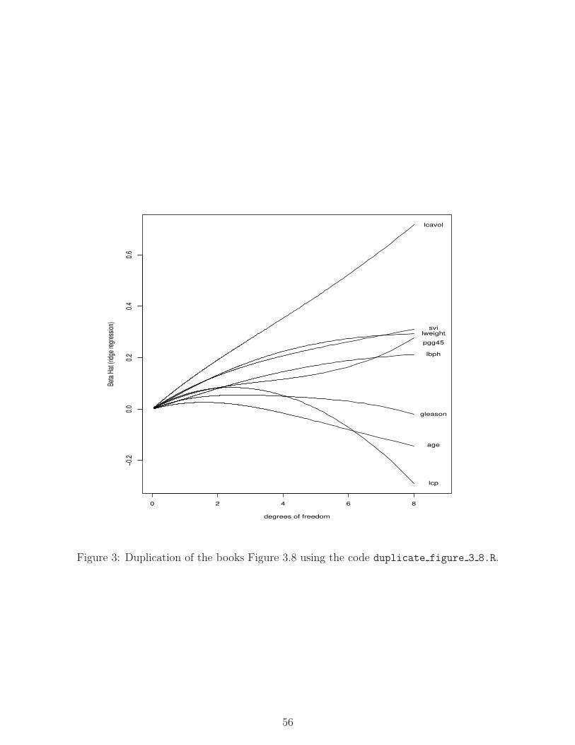
0 2 4 6 8
−0.2
0.0
0.2
0.4
0.6
degrees of freedom
Beta
Hat
(rid
ge re
gres
sion
)
lcavol
lweight
age
lbph
svi
lcp
gleason
pgg45
Figure 3: Duplication of the books Figure 3.8 using the code duplicate figure 3 8.R.
56

0.0 0.5 1.0 1.5 2.0
−0.2
0.0
0.2
0.4
0.6
L1 Norm
Coe
ffici
ents
0 2 5 7 7
Figure 4: Duplication of the books Figure 3.10 using the code dup OSE lasso.R. This plotmatches quite well qualitatively and quantitatively the corresponding one presented in thebook.
57

50 100 150 200 250
−0.2
0.0
0.2
0.4
0.6
Iteration
Coe
ffici
ents
lcavol
lweight
age
lbph
svi
lcp
gleason
pgg45
0 500 1000 1500 2000 2500
−0.2
0.0
0.2
0.4
0.6
Iteration
Coe
ffici
ents
lcavol
lweight
age
lbph
svi
lcp
gleason
pgg45
Figure 5: Numerical duplication of the books Figure 3.19. Left: Using the IncrementalForward Stagewise Regression (IFSR) with ǫ = 0.01 and 250 iterations of the algorithm.Right: IFSR with ǫ = 0.001 and 2500 iterations. With ǫ this small the curves are so smooththey approximate the lasso paths quite well.
58

−2 −1 0 1 2
−5
05
s
accura
te.y
Figure 6: The middle black curve is the curvey = 1.3965849 + 1.9407724x− 0.1215529x2 + 0.1535441x3.
The two red curves come from the upper and lower limits of the 95% confidence interval,taken separately at each value of x. The green curves are the result of sampling values fromthe boundary of the 4-dimensional 95% confidence region for values of β, as determined bythe χ2
4 distribution, and then drawing the corresponding curve. Note that the green curvesdo not lie entirely between the red curves.
59

−15 −10 −5 0 5 10 15
010
020
030
040
0
xx
(xx
− be
taH
at)^
2 +
lam
bda
* abs
(xx)
−15 −10 −5 0 5 10 15
050
100
150
200
250
300
xx
(xx
− be
taH
at)^
2 +
lam
bda
* abs
(xx)
−15 −10 −5 0 5 10 15
010
020
030
040
0
xx
(xx
− be
taH
at)^
2 +
lam
bda
* abs
(xx)
−15 −10 −5 0 5 10 15
050
100
150
200
250
300
xx
(xx
− be
taH
at)^
2 +
lam
bda
* abs
(xx)
Figure 7: Plots of (β − β)2 + λ|β| for various values of β and λ.Upper Left: For β = −5.0 and λ = 1.0. The minimum appears to be at β = −5.0.Upper Right: For β = −1.0 and λ = 5.0. The minimum appears to be at β = 0.0.Lower Left: For β = 5.0 and λ = 1.0. The minimum appears to be at β = 5.0.Lower Right: For β = 1.0 and λ = 5.0. The minimum appears to be at β = 0.0.
60

0 10 20 30 40 50
0.15
0.20
0.25
0.30
degrees of freedom
expe
cted s
quare
d pred
iction
error
(ESP
E)
−8 −7 −6 −5 −4 −3 −20.1
20.1
40.1
60.1
80.2
00.2
20.2
4
log(Lambda)
Mean
Squa
red Er
ror
56 56 55 55 55 54 52 51 48 44 40 34 26 24 15 8 5 1
0 10 20 30 40 50
0.15
0.20
0.25
0.30
degrees of freedom
expe
cted s
quare
d pred
iction
error
(ESP
E)
0 10 20 30 40 50
0.15
0.20
0.25
0.30
degrees of freedom
expe
cted s
quare
d pred
iction
error
(ESP
E)
Figure 8: Estimated prediction error curves and their standard errors for various linearmethods applied to the spam data set. From top to bottom, left to right the methodsdisplayed are: Ridge Regression, The Lasso, Principal Components Regression (PCR), andPartial Least Squares (PLS). The lasso results look different than that presented in thebook since we present the default plot result using the glmnet plot command. In addition,the PCR and PLS results don’t return cross validation results for the case of no predictors(predicting with the constant mean y only).
61

Chapter 4 (Linear Methods for Classification)
Notes on the Text
Notes on using LDA as a dimensionality reduction technique
In the R code dup fig 4.4.R we duplicate the results in the book where we project the voweldata set into a two dimensional space. When we run the above R code we get the resultshown in Figure 9. This result looks very much like the result presented in the book.
1 2 3 4
−5−4
−3−2
−10
Coordinate 1 for Training Data
Coo
rdin
ate
2 fo
r Tra
inin
g D
ata
Figure 9: Duplication of the books Figure 4.4 using the code dup fig 4 4.R.
Notes on Linear Discriminant Analysis
In this subsection of the book there were comments on a two class method for classificationthat was claimed to work quite well in practice. This novel method is based on an observation
62

made during the derivation of LDA in that the cut classification threshold point or the scalarvalue of the expression
1
2µT2 Σ
−1µ2 −1
2µT1 Σ
−1µ1 + log
(N1
N
)− log
(N2
N
), (78)
is only Bayes optimal when the two class conditional densities are Gaussian and have thesame covariance matrix. Thus the conclusion suggested by the authors is that one mightbe able to improve classification by specifying a different value for this cut point. In the R
function entitled two class LDA with optimal cut point.R we follow that suggestion anddetermine the cut point that minimizes the classification error rate over the training set. Wedo this by explicitly enumerating several possible cut points and evaluating the in-sampleerror rate of each parametrized classifier1. To determine the range of cut point to search forthis minimum over, we first estimate the common covariance matrix Σ, and the two classmeans µ1 and µ2 in the normal ways and then tabulate (over all of the training samples x)the left-hand-side of the book’s equation 4.11 or
xT Σ−1(µ2 − µ1) . (79)
Given the range of this expression we can sample cut points a number of times betweenthe minimum and maximum given value, classify the points with the given cut point andestimating the resulting classifier error rate. The above code then returns the cut pointthreshold that produces the minimum error rate over the in-sample data. This code is exer-cised using the R script two class LDA with optimal cut point run.R where we performpairwise classification on two vowels. While the book claimed that this method is often su-perior to direct use of LDA running the above script seems to indicate that the two methodsare very comparable. Running a pairwise comparison between the optimal cut point methodshows that it is only better then LDA 0.29 of the time. Additional tests on different datasets is certainly needed.
Regularized Discriminant Analysis
Some R code for performing regularized discriminant analysis can be found in rda.R. Thiscode is exercised (on the vowel data) in the R code dup fig 4 7.R which duplicates the plotgiven in the book. When that script is run we get
[1] "Min test error rate= 0.478355; alpha= 0.969697"
and the plot shown in Figure 10. This plot matches well with the one given in the book. Inaddition, we can shrink Σ towards a scalar and consider the more general three term model
Σk(α, γ) = αΣk + (1− α)(γΣ + (1− γ)σ2I) .
With this form for Σk we can again run a grid search over the parameters α and γ andselect values that optimize out of sample performance. When we do that (at the bottom ofthe dup fig 4 7.R) we get
1A better algorithm but one that requires more computation would be to specify the classification pointand estimate the error rate using leave-one-out cross-validation.
63

0.0 0.2 0.4 0.6 0.8 1.0
0.0
0.1
0.2
0.3
0.4
0.5
0.6
Duplication of Figure 4.7
alpha
erro
r rat
e
Figure 10: Duplication of the books Figure 4.7 using the code dup fig 4 7.R.
[1] "Min test error rate= 0.439394; alpha= 0.767677; gamma= 0.050505"
Notes on duplication of Table 4.1
In this dup table 4 1.R we call various R functions created to duplicate the results in thebook from Table 4.1. This code uses the R routine linear regression indicator matrix.R
which does classification based on linear regression (as presented in the introduction to thischapter). When we run that code we get results given by
64

Technique Training Test
[1] " Linear Regression: 0.477273; 0.666667"
[1] " Linear Discriminant Analysis (LDA): 0.316288; 0.556277"
[1] " Quadratic Discriminant Analysis (QDA): 0.011364; 0.528139"
[1] " Logistic Regression: 0.221591; 0.512987"
These results agree well with the ones given in the book.
Notes on Reduced-Rank Linear Discriminant Analysis
1 2 3 4
01
23
45
6
Coordinate 1 for Training Data
Coo
rdin
ate
2 fo
r Tra
inin
g D
ata
Figure 11: Duplication of the coordinate 1 - 7 projection found in the books Figure 4.8.
In this section of these notes we implement the reduced-rank linear discriminant analysis inthe R code reduced rank LDA.R. Using this code in the R code dup fig 4 8.R we can thenduplicate the projections presented in figure 4.8 from the book. When we run that code weget the plot given in Figure 11. This plot matches the results in the book quite well. In theR code dup fig 4.10.R we have code that duplicates figure 4.10 from the book. When thatcode is run we get the plot shown in Figure 12.
65

2 4 6 8 10
0.3
0.4
0.5
0.6
0.7
Dimension
Mis
clas
sific
atio
n ra
te
Figure 12: Duplication of the books Figure 4.10.
Logistic Regression
From the given specification of logistic regression we have
log
(Pr(G = 1|X = x)
Pr(G = K|X = x)
)= β10 + βT
1 x
log
(Pr(G = 2|X = x)
Pr(G = K|X = x)
)= β20 + βT
2 x
... (80)
log
(Pr(G = K − 1|X = x)
Pr(G = K|X = x)
)= β(K−1)0 + βT
K−1x .
The reason for starting with expressions of this form will become more clear when we look atthe log-likelihood that results when we use the multinomial distribution for the distributionsatisfied over the class of each sample once the probabilities Pr(G = k|X = x) are specified.Before we discuss that, however, lets manipulate the Equations 80 above by taking the theexponential of both sides and multiplying everything by Pr(G = K|X = x). When we do
66
this we find that these equations transform into
Pr(G = 1|X = x) = Pr(G = K|X = x) exp(β10 + βT1 x)
Pr(G = 2|X = x) = Pr(G = K|X = x) exp(β20 + βT2 x)
... (81)
Pr(G = K − 1|X = x) = Pr(G = K|X = x) exp(β(K−1)0 + βT(K−1)x) .
Adding the value of Pr(G = K|X = x) to both sides of the sum of all of the above equationsand enforcing the constraint that
∑l Pr(G = l|X = x) = 1, we find
Pr(G = K|X = x)
(1 +
K−1∑
l=1
exp(βl0 + βTl x)
)= 1 .
On solving for Pr(G = K|X = x) we find
Pr(G = K|X = x) =1
1 +∑K−1
l=1 exp(βl0 + βTl x)
. (82)
When we put this expression in the proceeding K − 1 in Equations 81 we find
Pr(G = k|X = x) =exp(βk0 + βT
k x)
1 +∑K−1
l=1 exp(βl0 + βTl x)
, (83)
which are equations 4.18 in the book.
Fitting Logistic Regression
In the case where we have only two classes, for the ith sample given the feature vectorX = xi the probability of that this sample comes from either of the two classes is givenby the two values of the posterior probabilities. That is given xi the probability we arelooking at a sample from the first class is Pr(G = 1|X = x), and from the second class isPr(G = 2|X = x) = 1 − Pr(G = 1|X = x). If for each sample xi for i = 1, 2, · · · , N inour training set we include with the measurement vector xi a “coding” variable denoted yi,that takes the value 1 if the ith item comes from the first class and is zero otherwise wecan succinctly represent the probability that xi is a member of its class with the followingnotation
pgi(xi) = Pr(G = 1|X = xi)yiPr(G = 2|X = x)1−yi . (84)
Since only one of the values yi or 1 − yi will in fact be non-zero. Using this notation givenan entire data set of measurements and their class encoding xi, yi the total likelihood ofthis data set is given by
L =N∏
i=1
pgi(xi) ,
the log-likelihood for this set of data is then given by taking the logarithm of this expressionas
l =
N∑
i=1
log(pgi(xi)) .
67

When we put in the expression for pgi(xi) defined in Equation 84 we obtain
l =
N∑
i=1
yi log(pgi(xi)) + (1− yi) log(1− pgi(xi))
=
N∑
i=1
y log
(pgi(xi)
1− pgi(xi)
)+ log(1− pgi(xi))
If we now use Equations 80 to express the log-posterior odds in terms of the parameters wedesire to estimate β we see that
log
(pgi(xi)
1− pgi(xi)
)= β10 + βT
1 = βTx ,
and
log(1− pgi(xi)) =1
1 + eβTx.
Here we have extended the definition of the vector x to include a constant value of one to dealnaturally with the constant value term β10. Thus in terms of β the log-likelihood becomes
l(β) =N∑
i=1
(yiβ
Txi − log(1 + eβT xi)).
Now to maximize the log-likelihood over our parameters β we need to take the derivative ofl with respect to β. We find
∂l(β)
∂β=
N∑
i=1
(yixi −
eβT xi
1 + eβT xixi
).
Since p(xi) =eβ
T xi
1+eβT xi
the score (or derivative of l with respect to β) becomes
∂l(β)
∂β=
N∑
i=1
xi(yi − p(xi)) . (85)
The score is a column vector and the Hessian or second derivative is a matrix. We candenote this notationally by taking the derivative ∂
∂βT of the score column vector (note the
transpose). We find
∂l(β)
∂β∂βT=
N∑
i=1
−xi
(∂p(xi)
∂βT
).
This expression in the summation is a row vector and is given by
∂p(xi)
∂βT=
eβT xi
1 + eβT xixTi − (eβ
Txi)2
(1 + eβT xi)2xTi = p(xi)(1− p(xi))x
Ti .
Thus we get
∂l(β)
∂β∂βT= −
N∑
i=1
xixTi p(xi)(1− p(xi)) , (86)
for the Hessian.
68

Notes on the South African heart disease data
In this dup table 4 2.R we call various R functions created to duplicate the results in thebook from Table 4.2. This gives a result that matches the books result quite well. Next inthe R code dup table 4 3.R we duplicate the results found in Table 4.3 in the book. Weuse the R function step to systematically remove predictors from the heart disease modelto end with the model chd ~ tobacco + ldl + famhist + age. After this model is foundthe step function tries to remove the remaining variables one at a time as can seen from thestep output
Step: AIC=495.44
chd ~ tobacco + ldl + famhist + age
Df Deviance AIC
<none> 485.44 495.44
- ldl 1 495.39 503.39
- tobacco 1 496.18 504.18
- famhist 1 502.82 510.82
- age 1 507.24 515.24
This shows that removing each of the three variables one at a time produces models thathave a larger Akaike information criterion (AIC) (and deviance) vs. the model above whereAIC = 495.44. Running the summary command on the resulting model gives
> summary(stepped_model)
Call:
glm(formula = chd ~ tobacco + ldl + famhist + age, family = binomial(),
data = SAheart)
Deviance Residuals:
Min 1Q Median 3Q Max
-1.7559 -0.8632 -0.4545 0.9457 2.4904
Coefficients:
Estimate Std. Error z value Pr(>|z|)
(Intercept) -4.204275 0.498315 -8.437 < 2e-16 ***
tobacco 0.080701 0.025514 3.163 0.00156 **
ldl 0.167584 0.054189 3.093 0.00198 **
famhistPresent 0.924117 0.223178 4.141 3.46e-05 ***
age 0.044042 0.009743 4.521 6.17e-06 ***
These results match well with the ones given in the book.
69

Notes on Optimal Separating Hyperplanes
For the Lagrange (primal) function to be minimized with respect to β and β0 given by
LP =1
2||β||2 −
N∑
i=1
αi[yi(xTi β + β0)− 1] , (87)
we have derivatives (set equal to zero) given by
∂Lp
∂β= β −
N∑
i=1
αiyixi = 0 (88)
∂Lp
∂β0= 0−
N∑
i=1
αiyi = 0 . (89)
Note that by expanding we can write Lp as
Lp =1
2||β||2 −
N∑
i=1
αiyixTi β − β0
N∑
i=1
αiyi +
N∑
i=1
αi .
From Equation 89 the third term in the above expression for Lp is zero. Using Equation 88to solve for β we find that the first term in the above expression for Lp is
||β||2 = βTβ =
(N∑
i=1
αiyixTi
)(N∑
j=1
αjyjxj
)=
N∑
i=1
N∑
j=1
αiαjyiyjxTi xj ,
and that the second terms in the expression for Lp is
N∑
i=1
αiyixTi β =
N∑
i=1
αiyixTi
(N∑
j=1
αjyjxj
)=
N∑
i=1
N∑
j=1
αiαjyiyjxTi xj .
Thus with these two substitutions the expression for Lp becomes (we now call this LD)
LD =N∑
i=1
αi −1
2
N∑
i=1
N∑
j=1
αiαjyiyjxTi xj . (90)
Exercise Solutions
Ex. 4.1 (a constrained maximization problem)
To solve constrained maximization or minimization problems we want to use the idea ofLagrangian multipliers. Define the Lagrangian L as
L(a;λ) = aTBa+ λ(aTWa− 1) .
70

Here λ is the Lagrange multiplier. Taking the a derivative of this expression and setting itequal to zeros gives
∂L(a;λ)∂a
= 2Ba+ λ(2Wa) = 0 .
This last equation is equivalent to
Ba + λWa = 0 ,
or multiplying by W−1 on both sides and moving the expression with B to the left hand sidegives the
W−1Ba = λa ,
Notice this is a standard eigenvalue problem, in that the solution vectors a must be aneigenvector of the matrix W−1B and λ is its corresponding eigenvalue. From the form of theobjective function we seek to maximize we would select a to be the eigenvector correspondingto the maximum eigenvalue.
Ex. 4.2 (two-class classification)
Part (a): Under zero-one classification loss, for each class ωk the Bayes’ discriminant func-tions δk(x) take the following form
δk(x) = ln(p(x|ωk)) + ln(πk) . (91)
If our conditional density p(x|ωk) is given by a multidimensional normal then its functionform is given by
p(x|ωk) = N (x;µk,Σk) ≡1
(2π)p/2|Σk|1/2exp
−1
2(x− µk)
TΣ−1k (x− µk)
. (92)
Taking the logarithm of this expression as required by Equation 91 we find
ln(p(x|ωk)) = −1
2(x− µk)
TΣ−1k (x− µk)−
p
2ln(2π)− 1
2ln(|Σk|) ,
so that our discriminant function in the case when p(x|ωk) is a multidimensional Gaussianis given by
δk(x) = −1
2(x− µk)
TΣ−1k (x− µk)−
p
2ln(2π)− 1
2ln(|Σk|) + ln(πk) . (93)
We will now consider some specializations of this expression for various possible values ofΣk and how these assumptions modify the expressions for δk(x). Since linear discriminantanalysis (LDA) corresponds to the case of equal covariance matrices our decision boundaries(given by Equation 93), but with equal covariances (Σk = Σ). For decision purposes we candrop the two terms −p
2ln(2π)− 1
2ln(|Σ|) and use a discriminant δk(x) given by
δk(x) = −1
2(x− µk)
TΣ−1(x− µk) + ln(πk) .
71

Expanding the quadratic in the above expression we get
δk(x) = −1
2
(xTΣ−1x− xTΣ−1µk − µT
kΣ−1x+ µT
kΣ−1µk
)+ ln(πk) .
Since xTΣ−1x is a common term with the same value in all discriminant functions we candrop it and just consider the discriminant given by
δk(x) =1
2xTΣ−1µk +
1
2µTkΣ
−1x− 1
2µTkΣ
−1µk + ln(πk) .
Since xTΣ−1µk is a scalar, its value is equal to the value of its transpose so
xTΣ−1µk =(xTΣ−1µk
)T= µT
k (Σ−1)Tx = µT
kΣ−1x ,
since Σ−1 is symmetric. Thus the two linear terms in the above combine and we are left with
δk(x) = xTΣ−1µk −1
2µTkΣ
−1µk + ln(πk) . (94)
Next we can estimate πk from data using πi =Ni
Nfor i = 1, 2 and we pick class 2 as the
classification outcome if δ2(x) > δ1(x) (and class 1 otherwise). This inequality can be writtenas
xTΣ−1µ2 −1
2µT2Σ
−1µ2 + ln(N2
N) > xTΣ−1µ1 −
1
2µT1Σ
−1µ1 + ln(N1
N) .
or moving all the x terms to one side
xTΣ−1(µ2 − µ1) >1
2µT1Σ
−1µ2 −1
2µT1Σ
−1µ1 + ln(N1
N)− ln(
N2
N) ,
as we were to show.
Part (b): To minimize the expression∑N
i=1(yi − β0 − βTxi)2 over (β0, β)
′ we know that the
solution (β0, β)′ must satisfy the normal equations which in this case is given by
XTX
[β0
β
]= XTy .
Our normal equations have a block matrix XTX on the left-hand-side given by
[1 1 · · · 1 1 1 · · · 1x1 x2 · · · xN1 xN1+1 xN1+2 · · · xN1+N2
]
1 xT1
1 xT2
...1 xT
N1
1 xTN1+1
1 xTN1+2
...1 xT
N1+N2
.
When we take the product of these two matrices we find
[N
∑Ni=1 x
Ti∑N
i=1 xi
∑Ni=1 xix
Ti
]. (95)
72

For the case where we code our response as − NN1
for the first class and + NN2
for the second
class (where N = N1 +N2), the right-hand-side or XTy of the normal equations becomes
[1 1 · · · 1 1 1 · · · 1x1 x2 · · · xN1 xN1+1 xN1+2 · · · xN1+N2
]
−N/N1
−N/N1...
−N/N1
N/N2
N/N2...
N/N2
.
When we take the product of these two matrices we get
N1
(− N
N1
)+N2
(NN2
)
(∑N1
i=1 xi
)(− N
N1
)+(∑N
i=N1+1 xi
)(NN2
)
=
[0
−Nµ1 +Nµ2
].
Note that we can simplify the (1, 2) and the (2, 1) elements in the block coefficient matrixXTX in Equation 95 by introducing the class specific means (denoted by µ1 and µ2) as
N∑
i=1
xi =
N1∑
i=1
xi +
N∑
i=N1+1
xi = N1µ1 +N2µ2 ,
Also if we pool all of the samples for this two class problem (K = 2) together we can estimatethe pooled covariance matrix Σ (see the section in the book on linear discriminant analysis)as
Σ =1
N −K
K∑
k=1
∑
i:gi=k
(xi − µk)(xi − µk)T .
When K = 2 this is
Σ =1
N − 2
[∑
i:gi=1
(xi − µ1)(xi − µ1)T +
∑
i:gi=2
(xi − µ2)(xi − µ2)T
]
=1
N − 2
[∑
i:gi=1
xixTi −N1µ1µ
T1 +
∑
i:gi=1
xixTi −N2µ2µ
T2
].
From which we see that the sum∑N
i=1 xixTi found in the (2, 2) element in the matrix from
Equation 95 can be written as
N∑
i=1
xixTi = (N − 2)Σ +N1µ1µ
T1 +N2µ2µ
T2 .
Now that we have evaluated both sides of the normal equations we can write them downagain as a linear system. We get
[N N1µ
T1 +N2µ
T2
N1µ1 +N2µ2 (N − 2)Σ +N1µ1µT1 +N2µ2µ
T2
] [β0
β
]=
[0
−Nµ1 +Nµ2
]. (96)
73

In more detail we can write out the first equation in the above system as
Nβ0 + (N1µT1 +N2µ
T2 )β = 0 ,
or solving for β0, in terms of β, we get
β0 =
(−N1
NµT1 − N2
NµT2
)β . (97)
When we put this value of β0 into the second equation in Equation 96 we find the totalequation for β then looks like
(N1µ1 +N2µ2)
(−N1
NµT1 − N2
NµT2
)β +
((N − 2)Σ +N1µ1µ
T1 +N2µ2µ
T2
)β = N(µ2 − µ1) .
Consider the terms that are outer products of the vectors µi (namely terms like µiµTj ) we
see that taken together they look like
Outer Product Terms = −N21
Nµ1µ
T1 − 2N1N2
Nµ1µ
T2 − N2
2
Nµ2µ
T2 +N1µ1µ
T2 +N2µ2µ
T2
=
(−N2
1
N+N1
)µ1µ
T1 − 2N1N2
Nµ1µ
T2 +
(−N2
2
N+N2
)µ2µ
T2
=N1
N(−N1 +N)µ1µ
T1 − 2N1N2
Nµ1µ
T2 +
N2
N(−N2 +N)µ2µ
T2
=N1N2
Nµ1µ
T1 − 2N1N2
Nµ1µ
T2 +
N2N1
Nµ2µ
T2
=N1N2
N(µ1µ
T1 − 2µ1µ2 − µ2µ2) =
N1N2
N(µ1 − µ2)(µ1 − µ2)
T .
Here we have used the fact that N1 +N2 = N . If we introduce the matrix ΣB as
ΣB ≡ (µ2 − µ1)(µ2 − µ1)T , (98)
we get that the equation for β looks like[(N − 2)Σ +
N1N2
NΣB
]β = N(µ2 − µ1) , (99)
as we were to show.
Part (c): Note that ΣBβ is (µ2 − µ1)(µ2 − µ1)Tβ, and the product (µ2 − µ1)
Tβ is a scalar.Therefore the vector direction of ΣBβ is given by µ2 − µ1. Thus in Equation 99 as both theright-hand-side and the term N1N2
NΣB are in the direction of µ2 − µ1 the solution β must be
in the direction (i.e. proportional to) Σ−1(µ2 − µ1).
Ex. 4.4 (multidimensional logistic regression)
In the case of K > 2 classes, in the same way as discussed in the section on fitting a logisticregression model, for each sample point with a given measurement vector x (here we are
74

implicitly considering one of the samples from our training set) we will associate a positioncoded response vector variable y of size K−1 where the l-th component of y is equal to oneif this sample is drawn from the l-th class and zero otherwise. That is
yi =
1 x is from class l and i = l0 otherwise
.
With this notation, the likelihood that this particular measured vector x is from its knownclass can be written as
py(x) = Pr(G = 1|X = x)y1Pr(G = 2|X = x)y2 · · ·Pr(G = K − 1|X = x)yK−1
× (1− Pr(G = 1|X = x)− Pr(G = 2|X = x)− · · · − Pr(G = K − 1|X = x))1−∑
K−1
l=1yl . (100)
Since this expression is for one data point the log-likelihood for an entire data set will begiven by
l =
N∑
i=1
log(pyi(xi)) .
Using the Equation 100 in the above expression we find log(py(x)) for any given trainingpair (xi,yi) is given by
log(py(x)) = y1 log(Pr(G = 1|X = x)) + y2 log(Pr(G = 2|X = x)) + · · ·+ yK−1 log(Pr(G = K − 1|X = x))
+ (1− y1 − y2 − · · · − yK−1) log(Pr(G = K|X = x))
= log(Pr(G = K|X = x))
+ y1 log
(Pr(G = 1|X = x)
Pr(G = K|X = x)
)+ y2 log
(Pr(G = 2|X = x)
Pr(G = K|X = x)
)+ · · ·+ yK−1 log
(Pr(G = K − 1|X = x)
Pr(G = K|X = x)
)
= log(Pr(G = K|X = x)) + y1(β01 + βT1 x) + y2(β02 + βT
2 x) + · · ·+ yK−1(β(K−1)0 + βTK−1x) .
The total log-likelihood is then given by summing the above expression over all data points
l(θ) =
N∑
i=1
[K−1∑
l=1
yilβTl xi + log(Pr(G = k|X = xi))
].
• Here xi is the ith vector sample 1 ≤ i ≤ N with a leading one prepended and so is oflength p+ 1.
• yil is the lth component of the ith response vector i.e. if the sample xi came from classl when 1 ≤ l ≤ K − 1 the lth element of yi is one and all the other elements are zero.If xi is a sample from class K then all elements of the vector yi are zero.
• βl is a vector of coefficients for the lth class 1 ≤ l ≤ K − 1 with the leading β0l
prepended and thus is of length p+ 1.
• Pr(G = k|X = xi) is the a posteriori probability that xi comes from class G = K andis given in terms of the parameters βlK−1
l=1 as
Pr(G = k|X = xi) =1
1 +∑K−1
l=1 exp(βTl xi)
.
75

• The total parameter set that we need to solve for of θ can be thought of as the “stacked”vector of β’s or
θ ≡
β1
β2...
βK−2
βK−1
,
this is a vector of size (K − 1)(p+ 1). Since each sub vector βl has p+ 1 components.
Using the expression for Pr(G = k|X = xi) the expression for l(θ) can be written as
l(θ) =
N∑
i=1
[K−1∑
l=1
yilβTl xi − log
(1 +
K−1∑
l=1
exp(βTl xi)
)].
Once we have the objective function l(θ) defined we can develop an algorithm to maximizeit l(θ) as a function of θ. To develop a procedure for this maximization we will use theNewton-Raphson algorithm in terms of θ (which is a block column vector in β) as
θnew = θold −(∂2l(θ)
∂θ∂θT
)−1∂l(θ)
∂θ. (101)
We need to evaluate the derivatives in the Newton-Raphson method. We will do this inblock form (which is the same way that θ is constructed). The expression ∂l(θ)
∂θis a block
vector with blocks given by the derivatives of l(θ) with respect to βl or
∂l(θ)
∂βl=
N∑
i=1
yilxi −exp(βT
l xi)
1 +∑K−1
l′=1 exp(βTl′ xi)
xi
=N∑
i=1
(yil − Pr(G = l|X = xi))xi .
The argument of the summation above are each column vectors of dimension p + 1 (since
the vectors xi are) and we to create the full vector ∂l(θ)∂θ
we would stack the K − 1 vectorsabove (one for each of l in 1 ≤ l ≤ K − 1) on top of each other. That is we form the full
gradient vector ∂l(θ)∂θ
as
∂l(θ)
∂θ=
∂l∂β1∂l∂β2
...∂l
∂βK−1
.
If we write the above βl derivative as two terms as
∂l(θ)
∂βl=
N∑
i=1
yilxi −N∑
i=1
Pr(G = l|X = xi)xi , (102)
76

and introduce the N × 1 column vectors tl and pl for 1 ≤ l ≤ K − 1 as
tl =
y1,ly2,l...
yN,l
and pl =
Pr(G = l|X = x1)Pr(G = l|X = x2)
...Pr(G = l|X = xN)
.
With these definitions we can then write ∂l(θ)∂βl
as
XT tl −XTpl = XT (tl − pl) .
The above can be verified by writing out components of the above products. When we stackthese vectors to form the full derivative we find
∂l(θ)
∂θ=
XT (t1 − p1)XT (t2 − p2)
...XT (tK−1 − pK−1)
=
XT 0 · · · 00 XT · · · 0...
.... . .
...0 0 · · · XT
t1 − p1
t2 − p2...
tK−1 − pK−1
. (103)
We see the appearance of a (K − 1)× (K − 1) block diagonal matrix with blocks given bythe (p+ 1)×N matrix XT . Lets denote this matrix by XT or
XT ≡
XT 0 · · · 00 XT · · · 0...
.... . .
...0 0 · · · XT
,
which we see is a (K − 1)(p+ 1)× (K − 1)N dimensioned matrix.
Next we have to evaluate the second derivative of l(θ). As we did when we evaluated the
first derivative we will evaluate this expression in block form. From the expression for ∂l(θ)∂βl
given in Equation 102 we have that
∂2l(θ)
∂βl∂βTl′= −
N∑
i=1
∂ Pr(G = l|X = xi)
∂βTl′
xi .
The above derivative on the right-hand-side depends on whether l = l′ or not. The casewhere l 6= l′ is slightly easier to compute and the derivative of Pr(G = l|X = xi) withrespect to βT
l′ in that case is
∂ Pr(G = l|X = xi)
∂βTl′
= Pr(G = l|X = xi) Pr(G = l′|X = xi)xTi .
From this we have that the block off-diagonal second derivative terms are given by
∂2l(θ)
∂βl∂βTl′= −
N∑
i=1
Pr(G = l|X = xi) Pr(G = l′|X = xi)xTi xi for l 6= l′ . (104)
77

Note that the right-hand-side of this expression evaluates to a (p + 1)× (p + 1) matrix (asit should). If l = l′ we find the derivative of Pr(G = l|X = xi) with respect to βT
l′ given by
∂ Pr(G = l|X = xi)
∂βTl′
=∂
∂βTl′
(eβl′xi
1 +∑K−1
l′′=1 eβl′xi
)
=eβl′xi
1 +∑K−1
l′′=1 eβl′xi
xi −eβl′xi
(1 +∑K−1
l′′=1 eβl′xi)2
eβl′xixi
= Pr(G = l′|X = xi)xi − Pr(G = l′|X = xi)2xi
= Pr(G = l′|X = xi)(1− Pr(G = l′|X = xi))xi .
From this we have that the block diagonal second derivative terms are given by
∂2l(θ)
∂βl∂βTl
= −N∑
i=1
Pr(G = l|X = xi)(1− Pr(G = l|X = xi))xTi xi . (105)
The right-hand-side of the above again evaluates to a (p+ 1)× (p+ 1) matrix. To computethe full Hessian we will assemble the block pieces (computed above) and form the full matrixas
∂2l(θ)
∂θ∂θT=
∂2l∂β1∂βT
1
∂2l∂βl∂β
T2
· · · ∂2l∂βl∂β
TK−1
∂2l∂β2∂βT
1
∂2l∂β2∂βT
2· · · ∂2l
∂β2∂βTK−1
......
. . ....
∂2l∂βK−1∂β
T1
∂2l∂βK−1∂β
T2
· · · ∂2l∂βK−1∂β
TK−1
.
As we did in the case of the first derivative of l(θ) we will write the second derivative of l(θ)in matrix notation. To do this, we first introduce K − 1, N × N diagonal matrices Ql for1 ≤ l ≤ K − 1 with diagonal elements given by Pr(G = l|X = xi)(1 − Pr(G = l|X = xi))where 1 ≤ i ≤ N . Then with these definitions we can write Equation 105 in matrix form by
∂2l(θ)
∂βl∂βTl
= −XTQlX .
We next introduce K − 1, N × N diagonal matrices Rl for 1 ≤ l ≤ K − 1 with diagonalelements given by Pr(G = l|X = xi) where 1 ≤ i ≤ N . Then with these definitions we canwrite Equation 104 in matrix form by
∂2l(θ)
∂βl∂βTl
= −XTRlRl′X .
With these definitions we get that the Hessian can be written as
∂2l(θ)
∂θ∂θT=
−XTQ1X −XTR1R2X · · · −XTR1RK−1X−XTR2R1X −XTQ2X · · · −XTR2RK−1X
.... . .
...−XTRK−1R1X −XTRK−1R2X · · · −XTQK−1X
This is a block (K − 1) × (K − 1) matrix with each block matrix of size (p + 1) × (p + 1)giving a total matrix size of (K − 1)(p+ 1)× (K − 1)(p+ 1). We can introduce the matrix
78

XT by writing the above Hessian as
∂2l(θ)
∂θ∂θT= −
XT 0 · · · 00 XT · · · 0...
.... . .
...0 0 · · · XT
Q1 R1R2 · · · R1RK−1
R2R1 Q2 · · · R2RK−1...
. . ....
RK−1R1 RK−1R2 · · · QK−1
X 0 · · · 00 X · · · 0...
.... . .
...0 0 · · · X
.
Define the non-diagonal matrix W as
W ≡
Q1 R1R2 · · · R1RK−1
R2R1 Q2 · · · R2RK−1...
. . ....
RK−1R1 RK−1R2 · · · QK−1
,
and we have∂2l(θ)
∂θ∂θT= −XTWX . (106)
Using Equation 103 and 106 we can write the Newton-Raphson method 101 for θ in matrixform in the same way as was done in the text for the two-class case. Namely we find
θnew = θold +(XTWX
)−1
XT
t1 − p1
t2 − p2...
tK−1 − pK−1
=(XTWX
)−1
XTW
Xθold +W−1
t1 − p1
t2 − p2...
tK−1 − pK−1
.
This shows that θnew is the solution of a non-diagonal weighted least squares problem witha response z given by
z ≡ Xθold +W−1
t1 − p1
t2 − p2...
tK−1 − pK−1
.
The fact that the weight matrix W is non-diagonal means that there are not efficient algo-rithms for solving the weighted least squares algorithm. In this case it is better perhaps toform the matrices above and to numerically adjust θ using the above matrix products start-ing at some initial value. Alternatively, another multidimensional optimization algorithmcould be used (rather than Newton-Raphson) for example the conjugate-gradient or Powell’smethod to find the optimal θ.
79

Ex. 4.6 (proving the convergence of the perceptron algorithm)
Part (a): By definition, if the points are separable then there exists a vector β such that
βTx∗i > 0 when yi = +1 and
βTx∗i < 0 when yi = −1 ,
for all i = 1, 2, · · · , N . This is equivalent to the expression that yiβTx∗
i > 0 for all i.Equivalently we can divide this expression by ||x∗
i || (a positive number) to get
yiβT zi > 0 ,
for all i. Since each one of these N values of yiβTzi is positive let m > 0 be the smallest
value of this product observed over all our training set. Thus by definition of m we have
yiβT zi ≥ m,
for all i. When we divide both sides of this inequality by this positive value of m we get
yi
(1
mβ
)T
zi ≥ 1 .
If we define βsep ≡ 1mβ we have shown that yiβ
Tsepzi ≥ 1 for all i.
Part (b): From βnew = βold + yizi we have that
βnew − βsep = βold − βsep + yizi .
When we square this result we get
||βnew − βsep||2 = ||βold − βsep||2 + y2i ||zi||2 + 2yi(βold − βsep)T zi .
Since yi = ±1 and ||zi||2 = 1 we have that y2i ||zi||2 = 1 for the second term on the right-hand-side. Note that the third term on the right-hand-side is given by
2(yiβToldzi − yiβ
Tsepzi) .
Since the “point” yi, zi was misclassified by the vector βold we have yiβToldzi < 0 (if it was
positive we would have classified it correctly). Since βsep is the vector that can correctlyclassify all points we have yiβ
Tsepzi ≥ 1. With these two facts we can write
2(yiβToldzi − yiβ
Tsepzi) ≤ 2(0− 1) = −2 .
Thus we have just shown that
||βnew − βsep||2 ≤ ||βold − βsep||2 + 1− 2 = ||βold − βsep||2 − 1 .
Thus we can drive any initial vector βstart to βsep in at most ||βstart − βsep||2 steps.
Ex. 4.9 (classification of the vowel data set)
See the notes on the text on Page 64 where a comparison of various classification methodson the vowel data set was done.
80

Chapter 5 (Basis Expansions and Regularization)
Notes on the Text
There is a nice chapter on using B-splines in the R language for regression problems in thebook [11]. There are several regression examples using real data and a discussion of thevarious decisions that need to be made when using splines for regression. The chapter alsoprovides explicit R code (and discussions) demonstrating how to solve a variety of appliedregression problems using splines.
Notes on piecewise polynomials and splines
If the basis functions hm(X) are local piecewise constants i.e. if
h1(X) = I(X < ξ1) , h2(X) = I(ξ1 ≤ X < ξ2) , h3(X) = I(ξ2 ≤ X) ,
and taking our approximation to f(X) of
f(X) ≈3∑
m=1
βmhm(X) ,
then the coefficients βm are given by solving the minimization problem
β = ArgMinβ
∣∣∣∣∣
∣∣∣∣∣f(X)−3∑
m=1
βmhm(X)
∣∣∣∣∣
∣∣∣∣∣
2
= ArgMinβ
∫ (f(x)−
3∑
m=1
βmhm(X)
)2
dX
= ArgMinβ
(∫ ξ1
ξL
(f(X)− β1)2dX +
∫ ξ2
ξ1
(f(X)− β2)2dX +
∫ ξR
ξ2
(f(X)− β3)2dX
).
Here ξL and ξR are the left and right end points of the functions domain. Since the above isa sum of three positive independent (with respect to βm) terms we can minimize the totalsum by minimizing each one independently. For example, we pick β1 that minimizes the firstterm by taking the derivative of that term with respect to β1, and setting the result equalto zero and solving for β1. We would have
d
dβ1
∫ ξ1
ξL
(f(X)− β1)2dX = 2
∫ ξ1
ξL
(f(X)− β1)dX = 0 .
When we solving this for β1 we get
β1 =1
ξ1 − ξL
∫ ξ1
ξL
f(X)dX = Y 1 ,
as claimed by the book. The other minimizations over β2 and β3 are done in the same way.
81

Note on R programming with splines
If one is working in the R language, much of the complexity of coding splines has already beendone by using the bs command (for B-splines) or the ns command (for natural splines). Forexample, if one has data in the vector X the following given various spline approximationsthat could be used as a first modeling attempt
• bs(x,degree=1,df=1) gives a single linear fit over the entire domain of X
• bs(x,degree=1,df=2) gives two linear fits with a break point at the median of thedata in X
• bs(x,degree=1,df=3) gives three linear fits separated at the 1/3 and 2/3 percentilepoints of the date
• bs(x,degree=2,df=2) gives a single quadratic fit over the entire domain
• bs(x,degree=2,df=3) gives two quadratic fits with a break point at the median ofthe data X
• bs(x,degree=2,df=4) gives three quadratic fits with a break points at the 1/3 and2/3 percentile points of the date
The way to reason about the values passed to each of the arguments of the bs functionsis that the degree argument is the degree of the polynomial that will be fit in each regionand that additional df values (above the minimum necessary) inserts additional polynomialsinto the domain. For example, to use linear fits requires degree=1 polynomials. Then thevalue of df must be at least one (for the slope) thus each additional value for df introducesa new region in which a line is fit. To use quadratic polynomials we use degree=2 and thendf must be larger than 2. As an example, in the R command dup fig 5 1.R we perform thesuggested fittings above on the function
Y = cos(X) + 0.3n .
where n ∼ N(0, 1). When that command is run we get the plots shown in Figure 13.
Notes on the South African Heart Disease Example
In the R code dup table 5 1.R we have code that duplicates logistic regression using theSouth African heart disease data. When we run that code we first fit a logistic regressionmodel and then use the R function step1 to experiment with removing various terms. Theoutput from this command gives
> drop1( m, scope=form, test="Chisq", data=SAheart )
Single term deletions
82

0 2 4 6 8 10 12
−1
.0−
0.5
0.0
0.5
1.0
x
y
0 2 4 6 8 10 12
−1
.0−
0.5
0.0
0.5
1.0
x
y
0 2 4 6 8 10 12
−1
.0−
0.5
0.0
0.5
1.0
x
y
0 2 4 6 8 10 12
−1
.0−
0.5
0.0
0.5
1.0
x
y
0 2 4 6 8 10 12
−1
.0−
0.5
0.0
0.5
1.0
x
y
0 2 4 6 8 10 12
−1
.0−
0.5
0.0
0.5
1.0
x
y
Figure 13: Piecewise regression using B-splines. The first row shows three linear models,while the second row shows three quadratic models.
83

0 50 100 150 200 250
05
10
15
20
25
Frequency
Log−
peri
odogra
m
0 50 100 150 200 250
−0.4
−0.2
0.0
0.2
0.4
Frequency
Logis
tic R
egre
ssio
n C
oeffic
ients
Figure 14: Duplication of plots in Figure 5.5 from the book.
Model:
chd ~ ns(sbp, df = 4) + ns(tobacco, df = 4) + ns(ldl, df = 4) +
famhist + ns(obesity, df = 4) + ns(alcohol, df = 4) + ns(age,
df = 4)
Df Deviance AIC LRT Pr(Chi)
<none> 457.63 509.63
ns(sbp, df = 4) 4 466.77 510.77 9.1429 0.0576257 .
ns(tobacco, df = 4) 4 469.61 513.61 11.9753 0.0175355 *
ns(ldl, df = 4) 4 470.90 514.90 13.2710 0.0100249 *
famhist 1 478.76 528.76 21.1319 4.287e-06 ***
ns(obesity, df = 4) 4 465.41 509.41 7.7749 0.1001811
ns(alcohol, df = 4) 4 458.09 502.09 0.4562 0.9776262
ns(age, df = 4) 4 480.37 524.37 22.7414 0.0001426 ***
These numbers match well with the ones given in the book.
Notes on the phoneme classification example
In the R code dup fig 5 5.R we duplicate some of the plots shown in the book. When werun that script we get the two plots shown in Figure 14. The error rate of the “raw” logisticregression classifier (without any smoothing) gives for training and testing
84

[1] "err_rate_train= 0.093114; err_rate_test= 0.24374"
These numbers are not that different for the ones given in the book. If we train a quadraticdiscriminant classifier on these two phonemes we get
[1] "err_rate_train= 0.000000; err_rate_test= 0.33941"
Finally, just to compare algorithms performance, we can fit (using cross validation) a regu-larized discriminant analysis model where we find
[1] "err_rate_train= 0.075781; err_rate_test= 0.19590"
the optimal parameters found were α = 0.1111111 and γ = 0.7474747. While this testingerror rate is not as good as the regularized result the book gives 0.158 regularized discriminantanalysis gives the best result of the three classifiers tested.
Notes on the bone mineral density (smoothing splines example)
In the R code dup fig 5 6.R we duplicate some of the plots shown in the book. When werun that script we get the two plots shown in Figure 15. This plot uses the R commandsmooth.spline.
Exercise Solutions
Ex. 5.1 (contributed by Mark-Jan Nederhof)
We can represent a cubic spline in two ways:
1. By the truncated power basis functions in (5.3).
2. By a collection of cubic functions, separated at the knots, such that in each knot, therelevant pair of functions has identical function values, and identical first and secondderivatives.
For this exercise we need to show that we can represent a function by (1) if and only ifwe can represent it by (2). The proof therefore distinguishes two directions. Here we onlyconsider the case of a single knot ξ. The proof is easily extended to having any number ofknots.
85

10 15 20 25
−0.05
0.00
0.05
0.10
0.15
0.20
Age
spnb
md
Figure 15: Duplication of plot in Figure 5.6 from the book.
We will use that for f(x) = (x−ξ)3 = x3−3ξx2+3ξ2x−ξ3, we have f(ξ) = f ′(ξ) = f ′′(ξ) = 0.Further, (x− ξ)3+ = 0 for x < ξ and (x− ξ)3+ = (x− ξ)3 for x ≥ ξ.
In the direction (1) → (2).
Consider h(x) = ax3 + bx2 + cx+ d+ e(x− ξ)3+. Now define:
h1(x) = ax3 + bx2 + cx+ d
h2(x) = ax3 + bx2 + cx+ d+ e(x− ξ)3
By expanding (x − ξ)3 = f(x) as cubic polynomial as above we immediately see that h2 isa cubic polynomial. Furthermore, h(x) = h1(x) for x < ξ, h(x) = h2(x) for x ≥ ξ, h2(ξ) =h1(ξ) + f(ξ) = h1(ξ), h
′2(ξ) = h′
1(ξ) + f ′(ξ) = h′1(ξ), and h′′
2(ξ) = h′′1(ξ) + f ′′(ξ) = h′′
1(ξ), asrequired.
In the direction (2) → (1).
Consider:
h(x) = h1(x) = a1x3 + b1x
2 + c1x+ d1 if x < ξ
h(x) = h2(x) = a2x3 + b2x
2 + c2x+ d2 if x ≥ ξ
such that h1(ξ) = h2(ξ), h′1(ξ) = h′
2(ξ), h′′1(ξ) = h′′
2(ξ), or in other words:
a1ξ3 + b1ξ
2 + c1ξ + d1 = a2ξ3 + b2ξ
2 + c2ξ + d2
3a1ξ2 + 2b1ξ + c1 = 3a2ξ
2 + 2b2ξ + c2
6a1ξ + 2b1 = 6a2ξ + 2b2
86

which means:
b2 − b1 = −3(a2 − a1)ξ
c2 − c1 = −3(a2 − a1)ξ2 − 2(b2 − b1)ξ =
= −3(a2 − a1)ξ2 + 6(a2 − a1)ξ
2 = 3(a2 − a1)ξ2
d2 − d1 = −(a2 − a1)ξ3 − (b2 − b1)ξ
2 − (c2 − c1)ξ =
= −(a2 − a1)ξ3 + 3(a2 − a1)ξ
3 − 3(a2 − a1)ξ3 = −(a2 − a1)ξ
3
Now let h(x) = h1(x) + (a2 − a1)(x− ξ)3+. If x < ξ then h(x) = h1(x) and if x ≥ ξ then:
h(x) = a1x3 + b1x
2 + c1x+ d1+
(a2 − a1)x3 − 3(a2 − a1)ξx
2 + 3(a2 − a1)ξ2x− (a2 − a1)ξ
3
= a1x3 + b1x
2 + c1x+ d1 + (a2 − a1)x3 + (b2 − b1)x
2 + (c2 − c1)x+ (d2 − d1)
= a2x3 + b2x
2 + c2x+ d2 = h2(x)
as required.
Ex. 5.2 (contributed by Mark-Jan Nederhof)
Part (a): We prove by induction Bi,m(x) = 0 for x /∈ [τi, τi+m).
Base for m = 1. By (5.77) Bi,1(x) = 0 for x /∈ [τi, τi+1).
Step from m − 1 to m. Suppose Bi,m−1(x) = 0 for x /∈ [τi, τi+m−1) and Bi+1,m−1(x) = 0 forx /∈ [τi+1, τi+1+m−1) = [τi+1, τi+m), then by (5.78) Bi,m(x) = 0 for x /∈ [τi, τi+m).
Part (b): We prove by induction Bi,m(x) > 0 for x ∈ (τi, τi+m).
Base for m = 1. By (5.77) Bi,1(x) > 0 for x ∈ (τi, τi+1).
Step from m − 1 to m. Suppose Bi,m−1(x) > 0 for x ∈ (τi, τi+m−1) and Bi+1,m−1(x) > 0 for
x ∈ (τi+1, τi+m). Notex−τi
τi+m−1−τi> 0 for x ∈ (τi, τi+m−1) and
τi+m−xτi+m−τi+1
> 0 for x ∈ (τi+1, τi+m).
Therefore by (5.78), Bi,m(x) > 0 for x ∈ (τi, τi+m).
Part (c): We prove by induction∑i
j=i−m+1Bj,m(x) = 1 for x ∈ [τi, τi+1).
Base for m = 1. This is immediate by (5.77).
Step from m− 1 to m. Suppose∑i
j=i−mBj,m−1(x) = 1 for x ∈ [τi, τi+1). By (5.78):
i∑
j=i−m+1
Bj,m(x) =i∑
j=i−m+1
[x− τj
τj+m−1 − τjBj,m−1(x) +
τj+m − x
τj+m − τj+1
Bj+1,m−1(x)
]
From (a), we know Bi−m+1,m−1(x) = 0 and Bi+1,m−1(x) = 0 for x ∈ [τi, τi+1). This meansthat for j = i −m + 1, the first term in the right-hand side above is 0, and for j = i, the
87

second term in the right-hand side is 0. For i−m ≤ j ≤ i, we combine the second term forj − 1 with the first term for j, to obtain:
i∑
j=i−m
[τj−1+m − x
τj−1+m − τj+
x− τjτj+m−1 − τj
]Bj,m−1(x) =
i∑
j=i−m
Bj,m−1(x) = 1
Part (d): Again easy induction suffices. For the base, (5.77) is piecewise polynomial of order0, and for the inductive step, (5.78) increases the order by 1, for each polynomial betweentwo consecutive knots, through the multiplication with x in the respective numerators.
Part (e): The claimed result does not seem to be true unless τi+1 = τi + 1, for all i, whichis known as a cardinal B-spline. In particular,
∫Bi,1(x)dx = τi+1− τi, and therefore Bi,1 can
be seen as a probability distribution if and only if τi+1 = τi + 1.
With cardinal B-splines in mind, let us define B1(x) = 1 if x ∈ [0, 1) and B1(x) = 0 otherwise.
For m > 1, we define Bm(x) =∫Bm−1(x− y)B1(y)dy =
∫ 1
0Bm−1(x− y)dy. This makes Bm
a convolution of m uniform random variables.
Let B′m denote the derivative of Bm as usual. For m ≤ 2 we will only consider the derivatives
in values of x that are not integers. Note that ∂∂yBm−1(x− y) = −B′
m−1(x− y) and thereforeby Leibniz’s integral rule:
B′m(x) =
∫ 1
0
B′m−1(x− y)dy = [−Bm−1(x− y)]10 = Bm−1(x)− Bm−1(x− 1)
It can be easily verified that:
B2(x) =
x for x ∈ [0, 1)2− x for x ∈ [1, 2)0 otherwise
(See also Figure 5.20 in the book.) This means:
B′2(x) =
1 for x ∈ (0, 1)−1 for x ∈ (1, 2)0 otherwise
Now we will prove by induction:
xB′m(x) = (m− 1)Bm(x)−mBm−1(x− 1) for m ≥ 2
Base for m = 2. We verify:
xB′2(x) =
x = B2(x)− 2B1(x− 1) = x− 2 · 0 for x ∈ (0, 1)−x = B2(x)− 2B1(x− 1) = 2− x− 2 · 1 for x ∈ (1, 2)0 otherwise
88

Step from m− 1 to m > 2. We have:
xB′m(x) =
∫ 1
0
xB′m−1(x− y)dy =
∫ 1
0
(x− y)B′m−1(x− y)dy +
∫ 1
0
yB′m−1(x− y)dy
Now use the inductive hypothesis on the first term in the right-hand side and integration byparts on the second term, to obtain:
∫ 1
0
(m− 2)Bm−1(x− y)− (m− 1)Bm−2(x− y − 1)dy+
[−yBm−1(x− y)]10 +
∫ 1
0
Bm−1(x− y)dy =
(m− 2)Bm(x)− (m− 1)Bm−1(x− 1)− Bm−1(x− 1) + Bm(x) =
(m− 1)Bm(x)−mBm−1(x− 1)
which completes the proof by induction.
We combine this with an earlier observation to give:
(m− 1)Bm(x)−mBm−1(x− 1) = xB′m(x) = xBm−1(x)− xBm−1(x− 1)
and hence:
Bm(x) =x
m− 1Bm−1(x) +
m− x
m− 1Bm−1(x− 1)
This is seen to be the same recurrence as (5.78) once we realize that Bi+1,m−1(x) = Bi,m−1(x−1) in the case of cardinal B-splines, that is, if τi+1 = τi + 1 for every i.
Ex. 5.4 (contributed by Mark-Jan Nederhof)
First we show (5.71). For x < ξ1, f(x) =∑3
j=0 βjxj and because f should be linear there,
we have β3 = 0 and β2 = 0. Similarly, for x ≥ ξK , f(x) =∑3
j=0 βjxj +∑K
k=1 θk(x− ξk)3 and
because f should be linear there, and because (x − ξk)3 = x3 − 3ξx2 + 3ξ2x − ξ3, we have
β3 +∑K
k=1 θk = 0 and β2 +∑K
k=1−3ξkθk = 0, which imply∑K
k=1 θk = 0 and∑K
k=1 ξkθk = 0.
To complete the exercise, we need to show that the following two ways of defining naturalcubic splines are equivalent:
1. By the basis in (5.4), with the definition in (5.5).
2. By the truncated power series representation in (5.70), with the natural boundaryconditions in (5.71).
In the direction (1) ⇒ (2). It is immediate that a function described using the basis in (5.4)can also be written in the form (5.70). What remains is to show that the natural boundary
89

conditions of (5.71) are satisfied. For x < ξ1, all Nk+2(x) are 0, so the function is linear. Forx ≥ ξK and k ≤ K − 2, Nk+2(x) evaluates to:
(x3 − 3ξkx2 + 3ξ2kx− ξ3k)− (x3 − 3ξKx
2 + 3ξ2Kx− ξ3K)
ξK − ξk−
(x3 − 3ξK−1x2 + 3ξ2K−1x− ξ3K−1)− (x3 − 3ξKx
2 + 3ξ2Kx− ξ3K)
ξK − ξK−1=
(−3ξk + 3ξK)
ξK − ξkx2 − (−3ξK−1 + 3ξK)
ξK − ξK−1x2 + C1x+ C0 = C1x+ C0
for constants C1 and C0, so that once more the function is linear.
In the direction (2) ⇒ (1). Assume a function is written as in (5.70) and (5.71). Then for thebasis in (5.4), the corresponding coefficient of Nk+2(x) is (ξK −ξk)θk for each k ≤ K−2, andobviously the coefficients of N1(x) and N2(x) are β0 and β1. Let us verify that we therebyobtain the same function, looking only at the coefficients of the Nk+2(x):
K−2∑
k=1
(ξK − ξk)θk
[(x− ξk)
3+ − (x− ξK)
3+
ξK − ξk− (x− ξK−1)
3+ − (x− ξK)
3+
ξK − ξK−1
]=
K−2∑
k=1
θk(x− ξk)3+ −
K−2∑
k=1
θk(x− ξK)3+−
1
ξK − ξK−1
[K−2∑
k=1
ξKθk −K−2∑
k=1
ξkθk
][(x− ξK−1)
3+ − (x− ξK)
3+
]
Now we make use of (5.71), in particular∑K−2
k=1 θk = −θK−1 − θK and∑K−2
k=1 ξkθk =−ξK−1θK−1 − ξKθK and obtain:
K−2∑
k=1
θk(x− ξk)3+ + (θK−1 + θK)(x− ξK)
3+−
1
ξK − ξK−1[−ξKθK−1 − ξKθK + ξK−1θK−1 + ξKθK ]
[(x− ξK−1)
3+ − (x− ξK)
3+
]=
K−2∑
k=1
θk(x− ξk)3+ + (θK−1 + θK)(x− ξK)
3+−
−ξKθK−1 + ξK−1θK−1
ξK − ξK−1
[(x− ξK−1)
3+ − (x− ξK)
3+
]=
K−2∑
k=1
θk(x− ξk)3+ + θK−1(x− ξK)
3+ + θK(x− ξK)
3+ + θK−1(x− ξK−1)
3+ − θK−1(x− ξK)
3+ =
K∑
k=1
θk(x− ξk)3+
as required.
90

Ex. 5.7 (contributed by Mark-Jan Nederhof)
Part (a): Using integration by parts:∫ b
a
g′′(x)h′′(x)dx = [g′′(x)h′(x)]ba −∫ b
a
g′′′(x)h′(x)dx
The first term on the right-hand side is 0 as g′′(a) = g′′(b) = 0. For the second term notethat g′′′(x) = 0 for x < x1 and for x ≥ xN . We break up the remaining interval into thepieces between consecutive knots, and once more apply integration by parts:
−N−1∑
i=1
∫ xi+1
xi
g′′′(x)h′(x)dx = −N−1∑
i=1
[g′′′(x)h(x)]xi+1xi
+
N−1∑
i=1
∫ xi+1
xi
g(4)(x)h(x)dx
The first term on the right-hand side is 0 as h(xi) = 0 for all i. The second term is 0 as well,as g(4)(x) = 0 for all x, since g is piecewise cubic.
Part (b): Using the result from (a):∫ b
a
g′′(t)2dt =
∫ b
a
(g′′(t) + h′′(t))2dt
=
∫ b
a
g′′(t)2dt+
∫ b
a
h′′(t)2dt+ 2
∫ b
a
g′′(t)h′′(t)dt
=
∫ b
a
g′′(t)2dt+
∫ b
a
h′′(t)2dt
Hence∫ b
ag′′(t)2dt ≥
∫ b
ag′′(t)2dt. Equality holds if and only if h′′(t) = 0 for all t ∈ [a, b],
which means h is linear in [a, b], and because h(xi) = 0 for all i and N ≥ 2, also h(t) = 0 forall t ∈ [a, b].
Part (c): Consider a minimizer f1. We can construct a natural cubic spline f2 with thesame function values in knots xi as f1, and therefore
∑i(yi − f1(xi))) =
∑i(yi − f2(xi))).
Because of minimality of f1 and because of (b), λ∫ b
af ′′1 (t)
2dt = λ∫ b
af ′′2 (t)
2dt and therebyf1 = f2.
Ex. 5.9 (deriving the Reinsch form)
GivenSλ = N(NTN + λΩN)
−1NT ,
when N is invertible then we have
Sλ = (N−T (NTN + λΩN )N−1)−1
= (N−TNTNN−1 + λN−TΩNN−1)−1
= (I + λN−TΩNN−1)−1 ,
so K ≡ N−TΩNN−1.
91

Chapter 6 (Kernel Smoothing Methods)
Ex. 6.1 (contributed by Mark-Jan Nederhof)
The Gaussian kernel is:
Kλ(x0, x) =1√2πλ
exp(−(x− x0)2
2λ2) (107)
We know the Gaussian kernel is differentiable, and therefore (6.2) with Kλ as above isdifferentiable. (One could use the quotient rule of differentiation to spell this out.)
For the Epanechnikov kernel, the above argument no longer works. In particular, for |t| = 1,i.e. for |x− x0| = λ > 0, we have d
dx0t2 = −2(x− x0) 6= 0.
For k-nearest neighborhoods an additional problem is that hk(x0) is not differentiable. Tosee this, take k+1 consecutive xi. Without loss of generality, assume these are x1, . . . , xk+1.Let x =
x1+xk+1
2. Now limx0↑x
ddx0
hk(x0) = 1, while limx0↓xd
dx0hk(x0) = −1.
Incidentally, the tri-cube kernel is differentiable, as D′(t) = 3(−3t2)(1− |t|3)2 for |t| ≤ 1, sofor |t| = 1 we have D′(t) = 0.
92
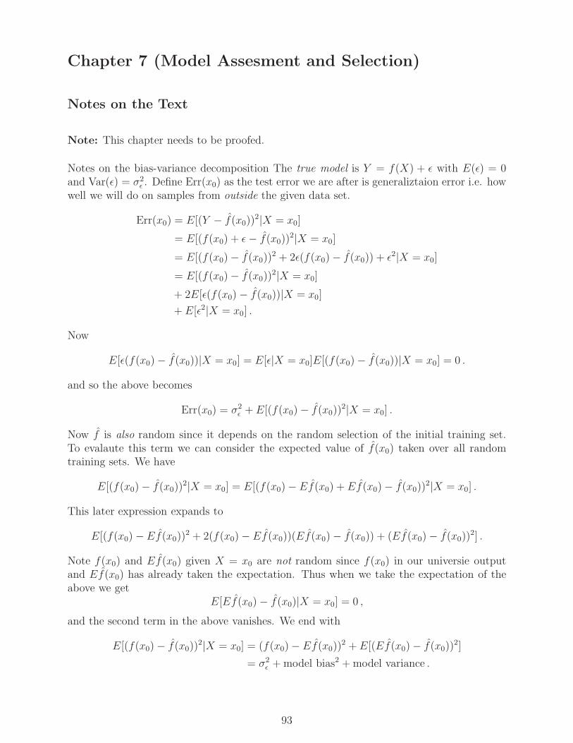
Chapter 7 (Model Assesment and Selection)
Notes on the Text
Note: This chapter needs to be proofed.
Notes on the bias-variance decomposition The true model is Y = f(X) + ǫ with E(ǫ) = 0and Var(ǫ) = σ2
ǫ . Define Err(x0) as the test error we are after is generaliztaion error i.e. howwell we will do on samples from outside the given data set.
Err(x0) = E[(Y − f(x0))2|X = x0]
= E[(f(x0) + ǫ− f(x0))2|X = x0]
= E[(f(x0)− f(x0))2 + 2ǫ(f(x0)− f(x0)) + ǫ2|X = x0]
= E[(f(x0)− f(x0))2|X = x0]
+ 2E[ǫ(f(x0)− f(x0))|X = x0]
+ E[ǫ2|X = x0] .
Now
E[ǫ(f(x0)− f(x0))|X = x0] = E[ǫ|X = x0]E[(f(x0)− f(x0))|X = x0] = 0 .
and so the above becomes
Err(x0) = σ2ǫ + E[(f(x0)− f(x0))
2|X = x0] .
Now f is also random since it depends on the random selection of the initial training set.To evalaute this term we can consider the expected value of f(x0) taken over all randomtraining sets. We have
E[(f(x0)− f(x0))2|X = x0] = E[(f(x0)− Ef(x0) + Ef(x0)− f(x0))
2|X = x0] .
This later expression expands to
E[(f(x0)−Ef(x0))2 + 2(f(x0)− Ef(x0))(Ef(x0)− f(x0)) + (Ef(x0)− f(x0))
2] .
Note f(x0) and Ef(x0) given X = x0 are not random since f(x0) in our universie outputand Ef(x0) has already taken the expectation. Thus when we take the expectation of theabove we get
E[Ef(x0)− f(x0)|X = x0] = 0 ,
and the second term in the above vanishes. We end with
E[(f(x0)− f(x0))2|X = x0] = (f(x0)− Ef(x0))
2 + E[(Ef(x0)− f(x0))2]
= σ2ǫ +model bias2 +model variance .
93

Y = f(X) + ǫ Var(ǫ) = σ2ǫ
Err(x0) = E[(Y − f(x0))2|X = x0]
= E[(f(x) + ǫ− f(x0))2|X = x0]
= E[(f(x)− f(x0) + ǫ)2|X = x0]
= E[(f(x0)− Ef(x0) + Ef(x0)− f(x0) + ǫ)2]
= E[(f(x0)− Ef(x0))2 + 2(f(x0)−Ef(x0))(Ef(x0)− f(x0)) + (Ef(x0)− f(x0))
2 + ǫ2]
We take the expectation over possible Y values via ǫ variabliligy and possible training setsthat go into constants of f(x0). Note that all E[(·)ǫ] = E[(·)]E[ǫ] = 0. The middle termsvanishes since E[f(x0)− Ef(x0)] = 0.
Introduce E[f(x0)] expected value over all training sets predicition using the median
For k nearest neighbor
f(x0) =1
k
k∑
l=1
f(x(l))
≈ 1
k
k∑
l=1
(f(x0) + ε(l)) = f(x0) +1
k
k∑
l=1
ε(l) .
Now the variance of the estimate f(x0) comes from the 1k
∑kl=1 ε(k) random term. Taking
the variance of this summation we have
1
k2
k∑
l=1
Var(ε(l)) =1
k2kVar(ε)
1
kσ2ε . (108)
Which is the equation in the book.
fp(x) = βTx we have
Err(x0) = E[(Y − fp(x0))2|X = x0]
= σ2ε + [f(x0)−Efp(x0)]
2 + ||h(x0||2σ2ε .
fp(x0) = xT0 (X
TX)−1XTy where y is random since y = y0 + ε
1
N
∑Err(x0) = σ2
ε +1
N
N∑
i=1
[f(xi)−Ef(xi)]2 +
p
Nσ2ε . (109)
94

Chapter 10 (Boosting and Additive Trees)
Notes on the Text
Notes on the Sample Classification Data
For AdaBoost.M1 the books suggests using a “toy” ten-dimensional data set where theindividual elements X1, X2, · · · , X10 of the vector X are standard independent Gaussianrandom draws and the classification labels (taken from −1,+1) are assigned as
Y =
+1 if
∑10j=1X
2j > χ2
10(0.5)
−1 otherwise.
Here χ210(0.5) is the median of a chi-squared random variable with 10 degrees of freedom.
In [2] it is stated that the Xi are standard independent Gaussian and their 10 values aresquared and then summed one gets a chi-squared random variable (by definition) with 10degrees of freedom. Thus the threshold chosen of χ2
10(0.5) since it is the median will splitthe data generated exactly (in the limit of infinite samples) into two equal sets. Thus whenwe ask for N samples we approximately equal number of N
2of samples in each class and
it is a good way to generate testing data. Code to generate data from this toy problemin Matlab is given by the function gen data pt b.m and in the R language in the functiongen eq 10 2 data.R.
Notes on duplicated Figure 10.2
See the R code dup fig 10 2.R where we use the R package gbm do duplicate the booksFigure 10.2. That package has an option (distribution=’adaboost’) that will performgradient boosting to minimize the exponential adaboost loss function. Since this packagedoes gradient boosting (a more general form of boosting) to get the results from the bookone needs to set the learning rate to be 1. When that code is run we get the results given inFigure 16, which matches quite well the similar plot given in the text. For a “home grown”Matlab implementation of AdaBoost see the problem on Page 103.
Notes on Why Exponential Loss
From the text and Equation 111 we have
f ∗(x) = argminf(x)EY |x(e−Y f(x)) =
1
2log
(Pr(Y = +1|x)Pr(Y = −1|x)
)
Solving the above for Pr(Y = +1|x) in terms of f ∗(x) we first write the above as
Pr(Y = +1|x)1− Pr(Y = +1|x) = e2f
∗(x) ,
95
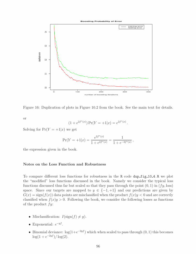
0 100 200 300 400
0.00.1
0.20.3
0.4
Boosting Probability of Error
number of boosting iterations
classi
fication
error
training errortesting error
Figure 16: Duplication of plots in Figure 10.2 from the book. See the main text for details.
or(1 + e2f
∗(x)) Pr(Y = +1|x) = e2f∗(x) .
Solving for Pr(Y = +1|x) we get
Pr(Y = +1|x) = e2f∗(x)
1 + e2f∗(x)=
1
1 + e−2f∗(x),
the expression given in the book.
Notes on the Loss Function and Robustness
To compare different loss functions for robustness in the R code dup fig 10 4.R we plotthe “modified” loss functions discussed in the book. Namely we consider the typical lossfunctions discussed thus far but scaled so that they pass through the point (0, 1) in (fy, loss)space. Since our targets are mapped to y ∈ −1,+1 and our predictions are given byG(x) = sign(f(x)) data points are misclassified when the product f(x)y < 0 and are correctlyclassified when f(x)y > 0. Following the book, we consider the following losses as functionsof the product fy:
• Misclassification: I(sign(f) 6= y).
• Exponential: e−yf .
• Binomial deviance: log(1+e−2yf ) which when scaled to pass through (0, 1) this becomeslog(1 + e−2yf )/ log(2).
96

• Squared error: (y − f)2 when scaled to pass through (0, 1) this becomes 1y2(1 − yf)2.
Note that we can drop the factor 1y2
since y ∈ −1,+1.
• Support vector (1− yf)+.
When we run the above R script we get the plot shown in Figure 17. Note that all curvesbut the one for binomial deviance (the orange curve) seem to be at their correct locations.There must be something wrong since the location of the binomial deviance curve in this plotwould indicate that binomial deviance is less robust to outlying classification examples thanis exponential loss (the cyan curve). This follows from the fact that the binomial deviancecurve lies above the exponential loss curve when yf < 0 indicating greater relative penaltyapplied when using the binomial deviance as a loss for incorrectly classified samples. This isin contrast to what the book states. There must be an error in this discussion but I’m notsure where it is. I’ve tried to “scale” the binomial functional form of log(1 + e−2yf ) by:
• Shifting the function along the fy axis
• Shifting the function along the loss axis
• Scaling the function by dividing by log(2)
and none of the resulting plots match the ones given in the book. Note that all of the abovetransformations pass through the point (0, 1). You can view the other plots by uncommentinglines in the dup fig 10 4.R script. If anyone sees a problem with my logic or knows what Iam doing incorrectly please contact me. For quadratic loss
f ∗(x) = argminf(x)EY |x(Y − f(x))2 = E(Y |x) ,
where the last step is via the Gauss Markov theorem (namely that the minimizer of thesquared error is the conditional expectation). Since the mapping for Y takes the form Y ∈−1,+1 we can evaluate the above expectation explicitly using the definition of expectation
E(Y |x) = +1Pr(Y = +1|x)− Pr(Y = −1|x)= +1Pr(Y = +1|x)− (1− Pr(Y = +1|x))= 2Pr(Y = +1|x)− 1 . (110)
Notes on Duplicating the Spam Data Example
See the R code dup spam classification.R where we use the R package gbm do duplicatethe books Spam data example. Following the documentation for the package gbm I selectedshrinkage=0.005 (a value be between 0.01 and 0.001), interaction.depth=1, cv.folds=5,and n.trees=50000 boosting trees to get estimate of the learning curves associated withthe gbm method applied to this data set. After training when one then calls the functiongbm.perf one gets the plot shown in Figure 18 (left) and the fact that the best number
97

−2 −1 0 1 2
0.00.5
1.01.5
2.02.5
3.0
y f
loss
Figure 17: An attempted duplication of plots in Figure 10.4 from the book. See the maintext for details.
of boosting trees is 10563. The error rate with this tree is 5.14%. This is a bit largerthan the numbers reported in the book but still in the same ballpark. If we retrain withinteraction.depth=3 we get the learning curve given in Figure 18 (right). The optimalnumber of boosting trees in this case 7417, also given a smaller testing error of 4.75%. TheR routine summary can be use to plot a relative importance graph. When we do that we getthe plot shown in Figure 19.
While the labeling of the above plot is not as good in the books we can print the first twentymost important words (in the order from most important to less important) to find
> most_important_words[1:20]
[1] "$" "!"
[3] "remove" "free"
[5] "hp" "your"
[7] "capital_run_length_average" "capital_run_length_longest"
[9] "george" "capital_run_length_total"
[11] "edu" "money"
[13] "our" "you"
[15] "internet" "1999"
[17] "will" "email"
[19] "re" "receive"
This ordering of words that are most important for the classification task agrees very wellwith the ones presented in the book.
98

0 10000 20000 30000 40000 50000
0.2
0.4
0.6
0.8
1.0
1.2
Iteration
Bern
oulli
devi
ance
0 10000 20000 30000 40000 50000
0.0
0.2
0.4
0.6
0.8
1.0
1.2
Iteration
Bern
oulli
devi
ance
Figure 18: Left: The learning curves of the gbm method on the spam data wheninteraction.depth=1. Note that after we have performed enough boosting iterations westeadily decrease the loss in sample (the black curve) while the loss out-of-sample staysnearly constant. Right: The learning curves of the gbm method on the spam data wheninteraction.depth=3. In this case as we perform learning by using more boosts we startto perform worse on the testing data set. This indicates that we are overfitting and learning(memorizing) the training data set. We should stop learning at the point where the errorwhen using the cross validation data set starts to increase i.e. the location of the minimumof the green curve. Note that the y-axis between the two plots are not the same.
99

$fre
ege
orge
our
1999
reme
eting
over
allord
erhp
lrep
ortcre
dit85
labs
415
0 20 40 60 80 100
Figure 19: A plot of the relative importance of the various words in the spam classificationexample using the R code summary(gbm).
Notes on Duplicating the Boosting with Different Sized Trees Example
See the R code dup fig 10 9.R where we use the R package gbm do duplicate the plot in thebook on comparing boosting with different sized trees. I could not get the gbm package toperform boosting with 100 node trees due to memory problems in the gbm package. I thinkthe book was using the MART package to do these plots and thus might have been able toperform boosting with these larger trees. The largest tree size I could boost with using gbm
was around 20. When I run the above script, I get the plot shown in Figure 20. This plotshows that AdaBoost and stumps seem to perform best on this problem in that they haveout of sample learning curves that continue to improve as we perform boosting iterations.Gradient boosting with 10 vs. 20 nodes seems to show qualitatively different behaviour. The10 node boosting algorithm seems to seem to be overfitting as we continue boosting, whileboosting with 20 node trees does not show this behaviour.
Exercise Solutions
Ex. 10.1 (deriving the β update equation)
From the book we have that for a fixed β the solution Gm(x) is given by
Gm = ArgMinG
N∑
i=1
w(m)i I(yi 6= G(xi)) ,
100

0 100 200 300 400
0.00.1
0.20.3
0.4
Boosting Probability of Error
number of boosting iterations
classi
fication
error
AdaBoostStumps10 Node20 Node
Figure 20: An attempted duplication of the Figure 10.9 from the book. The book’s learningcurve for AdaBoost does not perform as well as the result shown here.
which states that we should select our classifier Gm such that Gm(xi) = yi for the largest
weights w(m)i values, effectively “nulling” these values out. Now in AdaBoost this is done
by selecting the training samples according to a discrete distribution w(m)i specified on the
training data. Since Gm(x) is then specifically trained using these samples we expect thatit will correctly classify many of these points. Thus lets select the Gm(x) that appropriatelyminimizes the above expression. Once this Gm(x) has been selected we now seek to minimizeour exponential error with respect to the β parameter.
Then by considering Eq. 10.11 (rather than the recommended expression) with the derivedGm we have
(eβ − e−β)N∑
i=1
w(m)i I(yi 6= Gm(xi)) + e−β
N∑
i=1
w(m)i
Then to minimize this expression with respect to β, we will take the derivative with respectto β, set the resulting expression equal to zero and solve for β. The derivative (and settingour expression equal to zero) we find that
(eβ + e−β)N∑
i=1
w(m)i I(yi 6= Gm(xi))− e−β
N∑
i=1
w(m)i = 0 .
To facilitate solving for β we will multiply the expression above by eβ to give
(e2β + 1)
N∑
i=1
w(m)i I(yi 6= Gm(xi))−
N∑
i=1
w(m)i = 0 .
so that e2β is given by
e2β =
∑Ni=1w
(m)i −∑N
i=1w(m)i I(yi 6= Gm(xi))∑N
i=1w(m)i I(yi 6= Gm(xi))
.
101

Following the text we can define the error at the m-th stage (errm) as
errm =
∑Ni=1w
(m)i I(yi 6= Gm(xi))∑N
i=1w(m)i
,
so that in terms of this expression e2β becomes
e2β =1
errm− 1 =
1− errmerrm
.
Finally we have that β is given by
β =1
2log
(1− errmerrm
),
which is the expression Eq. 10.12 as desired.
Ex. 10.2 (minimize the AdaBoost loss)
We want to find f ∗(x) such that
f ∗(x) = argminf(x)EY |x(e−Y f(x)) .
To find f(x), we take the derivative of the above objective function with respect to f(x),set the resulting expression equal to zero, and solve for f(x). This procedure would give theequation
∂
∂fEY |x(e
−Y f(x)) = EY |x(−Y e−Y f(x)) = 0 .
Now evaluating the above expectation when our targets are Y = ±1 gives
−(−1)e−(−1)f(x)Pr(Y = −1|x)− 1(+1)e−f(x)Pr(Y = +1|x) = 0 .
Multiplying the above by ef(x) gives
e2f(x)Pr(Y = −1|x)− Pr(Y = +1|x) = 0 ,
or
e2f(x) =Pr(Y = +1|x)Pr(Y = −1|x) ,
or solving for f(x) we get
f(x) =1
2log
(Pr(Y = +1|x)Pr(Y = −1|x)
). (111)
the expression we were to show.
102

0 50 100 150 200 250 300 350 4000.1
0.15
0.2
0.25
0.3
0.35
0.4
0.45
0.5
training errtesting err
Figure 21: A duplication of the Figure 10.2 from the book.
Ex. 10.4 (Implementing AdaBoost with trees)
Part (a): Please see the web site for a suite of codes that implement AdaBoost with trees.These codes were written by Kelly Wallenstein under my guidance.
Part (b): Please see the Figure 21 for a plot of the training and test error using the provideAdaBoost Matlab code and the suggested data set. We see that the resulting plot looks verymuch like the on presented in Figure 10.2 of the book helping to verify that the algorithmis implemented correctly.
Part (c): I found that the algorithm proceeded to run for as long as I was able to wait.For example, Figure 21 has 800 boosting iterations which took about an hour train and testwith the Matlab code. As the number of boosting iterations increased I did not notice anysignificant rise in the test error. This was one of the purported advantages of the AdaBoostalgorithm.
Ex. 10.5 (Zhu’s multiclass exponential loss function)
Part (a): We want to find the vector function f ∗(x) such that
f ∗(x) = argminf(x)EY |x[L(Y, f)] = argminf(x)EY |x
[exp
(− 1
KY Tf
)],
103

and where the components of f(x) satisfy the constraint∑K
k=1 fk(x) = 0. To do this we willintroduce the Lagrangian L defined as
L(f ;λ) ≡ EY |x
[exp
(− 1
KY Tf
)]− λ
(K∑
k=1
fk − 0
).
Before applying the theory of continuous optimization to find the optima of L we will firstevaluate the expectation
E ≡ EY |x
[exp
(− 1
KY Tf
)].
Note that by expanding the inner products the above expectation can be written as
EY |x
[exp
(− 1
K(Y1f1 + Y2f2 + · · ·+ YK−1fK−1 + YKfK
)].
We then seek to evaluate the above expression by using the law of the unconscious statistician
E[f(X)] ≡∑
f(xi)p(xi) .
In the case we will evaluate the above under the encoding for the vector Y given by
Yk =
1 k = c
− 1K−1
k 6= c.
This states that when the true class of our sample x is from the class c, the response vectorY under this encoding has a value of 1 in the c-th component and the value − 1
K−1in all
other components. Using this we get the conditional expectation given by
E = exp
− 1
K
(− 1
K − 1f1(x) + f2(x) + · · ·+ fK−1(x) + fK(x)
)Prob(c = 1|x)
+ exp
− 1
K
(f1(x)−
1
K − 1f2(x) + · · ·+ fK−1(x) + fK(x)
)Prob(c = 2|x)
...
+ exp
− 1
K
(f1(x) + f2(x) + · · · − 1
K − 1fK−1(x) + fK(x)
)Prob(c = K − 1|x)
+ exp
− 1
K
(f1(x) + f2(x) + · · ·+ fK−1(x)−
1
K − 1fK(x)
)Prob(c = K|x) .
Now in the exponential arguments in each of the terms above by using the relationship
− 1
K − 1=
K − 1−K
K − 1= 1− 1
K − 1,
we can write the above as
E = exp
− 1
K
(f1(x) + f2(x) + · · ·+ fK−1(x) + fK(x)−
K
K − 1f1(x)
)Prob(c = 1|x)
+ exp
− 1
K
(f1(x) + f2(x) + · · ·+ fK−1(x) + fK(x)−
K
K − 1f2(x)
)Prob(c = 2|x)
...
+ exp
− 1
K
(f1(x) + f2(x) + · · ·+ fK−1(x) + fK(x)−
K
K − 1fK−1(x)
)Prob(c = K − 1|x)
+ exp
− 1
K
(f1(x) + f2(x) + · · ·+ fK−1(x) + fK(x)−
K
K − 1fK(x)
)Prob(c = K|x) .
104

Using the constraint is∑K
k′=1 fk′(x) = 0 the above simplifies to
E = exp
1
K − 1f1(x)
Prob(c = 1|x) + exp
1
K − 1f2(x)
Prob(c = 2|x)
...
+ exp
1
K − 1fK−1(x)
Prob(c = K − 1|x) + exp
1
K − 1fK(x)
Prob(c = K|x) .
Then to find the vector f(x), we take the derivative of the Lagrangian objective function Lwith respect to each component fk(x) (and the Lagrangian multiplier λ), set the resultingexpressions equal to zero, and solve the resulting system of equations for fk(x). Recall thatto get the full function form for L we need to add −λ
∑Kk=1 fk to E . With this the derivative
with respect to fk(x) of our Lagrangian gives
∂L∂fk
=∂E∂fk
− λ =1
K − 1exp
1
K − 1fk(x)
Prob(c = k|x)− λ , (112)
for 1 ≤ k ≤ K. The derivative of the Lagrangian with respect to λ gives back the constrainequation
∑Kk′=1 fk′(x) = 0. To solve these equations we will solve each of Equation 112 for
fk(x) in terms of λ and then put these equations back into the constraint that all fk mustsum to zero. We find that fk(x) in terms of λ is given by
fk(x) = −(K − 1) log
( −(K − 1)λ
Prob(c = k|x)
),
orfk(x) = −(K − 1) log(Prob(c = k|x))− (K − 1) log(−(K − 1)λ) . (113)
Enforcing that this expression must sum to zero means that
(K − 1)
K∑
k′=1
log(Prob(c = k′|x))−K(K − 1) log(−(K − 1)λ) = 0 .
If we divide by (K − 1)K we get
log(−(K − 1)λ) =1
K
K∑
k′=1
log(Prob(c = k′|x)) ,
or solving for λ we get
λ = − 1
K − 1exp
(1
K
K∑
k′=1
log(Prob(c = k′|x)))
.
When we put this expression for λ in Equation 113 we get
fk(x) = (K − 1) log(Prob(c = k|x))− K − 1
K
K∑
k′=1
log(Prob(c = k′|x))
= (K − 1)
(log(Prob(c = k|x))− 1
K
K∑
k′=1
log(Prob(c = k′|x))
,
105

for 1 ≤ k ≤ K. We can view the above as K equations for the K unknowns Prob(c = k|x).To find these probabilities in terms of fk(x) we first write the above as
1
K − 1fk(x) = log(Prob(c = k|x)) + log
[
K∏
k′=1
Prob(c = k′|x)]−1/K
.
From this we can solve for Prob(c = k|x) to get
Prob(c = k|x) =[
K∏
k′=1
Prob(c = k′|x)]1/K
efk(x)
K−1 . (114)
If we sum both sides of this equation from k′ = 1 to k′ = K the left-hand-side must sum toone, the term in brackets is constant with respect to the summation index, and we get
1 =
[K∏
k′=1
Prob(c = k′|x)]1/K K∑
k′=1
efk′
(x)
K−1 .
Using this expression we can solve for the term in brackets to find
[K∏
k′=1
Prob(c = k′|x)]1/K
=1
∑Kk′=1 e
fk′
(x)
K−1
.
Using this expression in Equation 114 we get
Prob(c = k|x) = efk(x)
K−1
∑Kk′=1 e
fk′
(x)
K−1
,
one of the desired expressions.
Ex. 10.7 (the optimal offset γjm)
We want to find the optimal constants γjm in each region of the tree. We have
γjm = argminγjm
∑
xi∈Rjm
L(yi, fm−1(xi) + γjm)
= argminγjm
∑
xi∈Rjm
e−yifm−1(xi)−yiγjm since we assume exponential loss
= argminγjm
∑
xi∈Rjm
w(m)i e−yiγjm since w
(m)i ≡ e−yifm−1(xi) .
Define a function of γjm by
F (γjm) ≡∑
xi∈Rjm
w(m)i e−yiγjm ,
106

then to find the minimum of this we solve
F ′(γjm) =∑
xi∈Rjm
w(m)i e−yiγjm(−yi) = 0 .
We can write the above summation in two parts by introducing indicator functions. Whenwe use these the above equation can be written as
−∑
xi∈Rjm
w(m)i e−γjmI(yi = +1) +
∑
xi∈Rjm
w(m)i eγjmI(yi = −1) = 0 .
Notice that eγjm in the sums above are independent of the summation index. Next multiplythe above equation by eγjm to get
e2γjm∑
xi∈Rjm
w(m)i I(yi = −1) =
∑
xi∈Rjm
w(m)i I(yi = +1) ,
or solving for γjm we find
γjm =1
2log
(∑xi∈Rjm
w(m)i I(yi = +1)
∑xi∈Rjm
w(m)i I(yi = −1)
).
Note that in the above I have a factor of 1/2 that the book does not have. Note also that afactor of 1/2 appears in a similar calculation that results in Equation 111. I wonder if thismissing 1/2 in the book might be a typo. If anyone sees anything wrong with what I havedone please contact me.
Ex. 10.8
Part (a): Note that if we approximate the class conditional probabilities using
pk(x) =efk(x)
∑Kl=1 e
fl(x), (115)
then pk(x) > 0 and∑K
k=1 pk(x) = 1 as required for a probability model. Note that asspecified there is redundancy in this model since we can add an arbitrary function h(x)to each function fk(x) and the value of pk(x) does not change. Thus we will impose theconstraint that
∑Kl=1 fl(x) = 0 to eliminate this redundancy. For this problem we are asked
to consider the log-likelihood (which is the negative multinomial deviance) and is specifiedin the book. For a single training example the log-likelihood is given by
L(y, p(x)) =
K∑
k=1
I(y = Gk) log(pk(x)) =
K∑
k=1
I(y = Gk)fk(x)− log
(K∑
l=1
efl(x)
). (116)
Part (b): If in the region R we want to increment fk(x) by some amount γk we shouldconsider the total log-likelihood over all samples in the region R and the total log-likelihoodthen becomes (using the encoding of y specified)
LL ≡∑
xi∈R
K∑
k=1
yikfk(xi)−∑
xi∈R
log
(K∑
l=1
efl(xi)
).
107

When we increment fk(x) by γk our log-likelihood becomes
LL(γ) =∑
xi∈R
K∑
k=1
yik(fk(xi) + γk)−∑
xi∈R
log
(K∑
l=1
efl(xi)+γl
).
As we are going to use Newton’s algorithm to find the maximum of the log-likelihood (orthe minimum of the deviance) with respect to the K − 1 values γk (the Kth value is takento be zero) we will need to evaluate the first and second derivatives of LL with respect tothese variables. We find
∂
∂γkLL(γ) =
∑
xi∈R
yik −∑
xi∈R
(efk(xi)+γk
∑Kl=1 e
fl(xi)+γl
),
for 1 ≤ k ≤ K− 1. Next we need to take the derivative of the above with respect to γk′. Wehave two cases to consider, when k′ = k and when k′ 6= k. We find when k′ 6= k that
∂2
∂γk∂γk′LL(γ) = −
∑
xi∈R
efk(x)+γkefk′ (x)+γk′
(∑Kl=1 e
fl(xi)+γl
)2 ,
and when k′ = k that
∂2
∂γk∂γkLL(γ) =
∑
xi∈R
− e2fk(x)+2γk
(∑Kl=1 e
fl(xi)+γl
)2 +efk(x)+γk
(∑Kl=1 e
fl(xi)+γl
)
,
One step of Newton’s method will start with a value for γ0 and update to get γ1 using
γ1 = γ0 −[∂2LL(γ)
∂γk∂γk′
]−1∂LL(γ)
∂γk.
If we start our Newton iterations with γ0 = 0 then the gradient and the Hessian simplify.We find
∂
∂γkLL(γ = 0) =
∑
xi∈R
yik −∑
xi∈R
pik =∑
xi∈R
(yik − pik)
∂2
∂γk∂γk′LL(γ = 0) = −
∑
xi∈R
pikpik′ for k′ 6= k
∂2
∂γk∂γkLL(γ = 0) =
∑
xi∈R
(−p2ik + pik) for k′ = k .
Here we have defined pik = efk(xi)∑K
l=1 fl(xi). If we assume that the Hessian is diagonal the the
matrix inverse becomes a sequence of scalar inverses, and our first Newton iterations become
γ1k =
∑xi∈R
(yik − pik)∑xi∈R
pik(1− pik),
for 1 ≤ k ≤ K − 1.
108

Part (c): The above update will produce values of γ1k that do not sum to zero as our original
functions fk(x) do. I’m not sure how to argue using symmetry for the formula given in thebook. It is easy to show that the formula suggested does satisfy the desired requirementthat
∑Kk=1 γk = 0 by simply summing each of the terms. If you assume that the form for the
normalized gammas, i.e. γk, is an affine function of first Newton update γ1k namely
γk = aγ1k + b ,
then to make sure that γk sums to zero requires that
K∑
k=1
γk = aK∑
k=1
γ1k + bK = 0 so b = − a
K
K∑
k=1
γ1k .
Thus we have shown that
γk = a
[γ1k −
1
K
K∑
k=1
γ1k
],
but I’m not sure how to argue for the expression given in the book for a. If anyone knowsan argument for why the given expression is a good one to use please contact me.
109

Chapter 14 (Unsupervised Learning)
Notes on the Text
Notes on Unsupervised as Supervised Learning
I believe there is a slight typo in this section of the book or at least the results they presentare valid for the case where we duplicate (using the proposed density g0(x) exactly the samenumber of cases as we are presented with originally, that is N0 = N . If we do actually onlygenerate N0 6= N cases from g0(x) then defining w = N
N0+Nand w0 = N0
N0+Nthe density of
points x should be given by the two component mixture model
f(x) = wg(x) + w0g0(x) .
Then the expression for µ(x) = E(Y |x) is given by
µ(x) = E(Y |x) = 0P (Y = 0|x) + 1P (Y = 1|x) = P (Y = 1|x)
=P (x|Y = 1)P (Y = 1)
P (x)=
g(x)w
wg(x) + w0g0(x)
=g(x)
g(x) +(w0
w
)g0(x)
.
Note this equals the result in the book if N0 = N .
Notes on Object Dissimilarity
From the definition of dj of
dj =1
N2
N∑
i=1
N∑
i′=1
(xij − xi′j)2 ,
we can transform this to an expression relating dj to the variance of xj . To do this we firstexpand the quadratic in the double summation and write dj as
dj =1
N2
N∑
i=1
N∑
i′=1
(x2ij − 2xi′jxij + x2
i′j)
=1
N2
N∑
i=1
N∑
i′=1
x2ij −
2
N2(N2x2
j ) +1
N2
N∑
i=1
N∑
i′=1
x2i′j
=1
N
N∑
i=1
x2ij − 2x2
j +1
N
N∑
i′=1
x2i′j .
110

To continue, recall that if X is a random variable with N samples xi then one can show that
Var(X) =1
N
N∑
i=1
xi2 −
(1
N
N∑
i=1
xi
)2
=1
N
N∑
i=1
xi2 − x2 ,
so that1
N
N∑
i=1
x2i = Var(X) + x2 .
Thus using this we see that dj can be written as
dj = Var(xj) + xj − 2x2j +Var(xj) + xj = 2Var(xj) , (117)
as claimed in the books equation 14.27.
Notes on the k-means algorithm
Recall the definition of W (C)
W (C) =1
2
K∑
k=1
∑
C(i)=k
∑
C(i′)=k
||xi − xi′ ||2 , (118)
then since||xi − xi′ ||2 = (xi − xi′)
T (xi − xi′) = xTi xi − 2xT
i xi′ + xTi′xi′ ,
then we can write∑
C(i′)=k ||xi − xi′ ||2 as
∑
C(i′)=k
(xTi xi − 2xT
i xi′ + xTi′xi′) = Nkx
Ti xi − 2xT
i (Nkxk) +∑
C(i′)=k
xTi′xi′ .
Next perform the summation of this expression over the points xi such that C(i) = k to get
Nk
∑
C(i)=k
xTi xi − 2(Nkxk)
T (Nkxk) +Nk
∑
C(i′)=k
xTi′xi′ = 2Nk
∑
C(i)=k
xTi xi −Nkx
Tk xk
. (119)
We would like to show that the expression in brackets is equal to∑
C(i)=k ||xi − xk||2. To dothat we next consider
∑
C(i)=k
||xi − xk||2 =∑
C(i)=k
(xTi xi − 2xT
i xk + xTk x)
=∑
C(i)=k
xTi xi − 2(Nkxk)
T xk +NkxTk xk
=∑
C(i)=k
xTi xi −Nkx
Tk xk ,
111

so they are equal. Putting∑
C(i)=k ||xi − xk||2 where the expression in brackets is in Equa-tion 119, and then into Equation 118 we find
W (C) =
K∑
k=1
Nk
∑
C(i)=k
||xi − xk||2 , (120)
which is the books equation 14.31.
The book also claims that the solution m to the following minimization problem
argminm
∑
i∈S
||xi −m||2
is xS or the mean over the points in the set S. This can be shown by defining f(m) ≡∑i∈S ||xi−m||2 taking the derivative with respect to m, setting the result equal to zero and
then solving for m. Recalling that
∂
∂m(xi −m)TA(xi −m) = −(A + AT )(xi −m) ,
so ∂∂m
∑i∈S ||xi −m||2 is given by
−2∑
i∈S
(xi −m) .
When we set this expression equal to zero and solve for m we have∑
i∈S
xi =∑
i∈S
m = |S|m,
or
m =1
|S|∑
i∈S
xi = xS ,
showing the claimed result. Here we have denoted |S| the number of points in the set S.
Exercise Solutions
Ex. 14.1 (the weighted Euclidean distance)
Consider the expression for d(w)e (xi, x
′i). We see that
d(w)e (xi, x
′i) =
∑pl=1wl(xil − xi′l)
2
∑pl=1wl
=
p∑
l=1
(wl∑pl=1wl
)(xil − xi′l)
2 .
Define sl =wl∑pl=1 wl
then the above can be written as
d(w)e (xi, x
′i) =
p∑
l=1
(√slxil −
√slxi′l)
2 .
112

If we define vectors zi with components given by
zil = xil
√sl = xil
(wl∑pl=1wl
)1/2
,
then the above shows that d(w)e (xi, x
′i) is equal to de(zi, z
′i) as we were to show.
Ex. 14.2 (k-means as the EM algorithm)
Part 1: The likelihood function for the data set xiNi=1 is given by
N∏
i=1
g(xi) =
N∏
i=1
(K∑
k=1
πkgk(x)
).
The loglikelihood is then given by
N∑
i=1
log
(K∑
k=1
πkgk(x)
).
Ex. 14.5 (k-means and the SOM algorithm on some semi-spherical data)
Since the R programming envionment provides a function for k-means (called kmean) and afunction for Kohonen’s self-organizing maps (called SOM) we will use these functions to studythis problem.
Ex. 14.6 (k-means and the SOM algorithm on the tumor microarray data)
Ex. 14.7 (PC minimization)
We want to find µ and Vq that minimize
N∑
i=1
||xi − µ− Vqλi||2 . (121)
We take the derivative with respect to µ, set the result equal to zero, and solve for µ. Wefind this derivative given by
∂
∂µ
(N∑
i=1
(xi − µ− Vqλi)T (xi − µ− Vqλi)
)=
N∑
i=1
−2(xi − µ− Vqλi) .
113

Setting this equal to zero and solving for µ we find
µ = x− Vq
(1
N
N∑
i=1
λi
), (122)
where x = 1N
∑Ni=1 xi. Next we take the derivative of Equation 121, with respect to λi, set
the result equal to zero and then solve for λi. To do this we write the sum in Equation 121as
N∑
i=1
[(xi − µ)T − 2(xi − µ)TVqλi + λTi V
Tq Vqλi] .
From which we see that taking, the ∂∂λi
derivative of this expression and setting the resultequal to zero is given by
−2((xi − µ)TVq)T ++(V T
q Vq + V Tq Vq)λi = 0 ,
orV Tq (xi − µ) = V T
q Vqλi = λi , (123)
since V Tq Vq = Ip. When we put this value of λi into Equation 122 to get
µ = x− VqVTq (x− µ) .
Thus µ must satisfyVqV
Tq (x− µ) = x− µ ,
or(I − VqV
Tq )(x− µ) = 0 .
Now I − VqVTq is the orthogonal projection onto the subspace spanned by the columns of Vq
thus µ = x+ h, where h is an arbitray p dimensional vector in the subspace spanned by Vq.Since Vq has a rank of q the vector h is selected from an p− q dimensional space (the spacespanned by the orthogonal complement of the columns of Vq). If we take h = 0 then µ = xand we get
λi = V Tq (xi − x) ,
from Equation 123.
Ex. 14.8 (the procrustes transformation)
For the Procrustes transformation we want to evaluate
argminµ,R||X2 − (X1R + 1µT )||F . (124)
This has the same solution when we square the same norm as above
argminµ,R||X2 − (X1R + 1µT )||2F .
When we use the fact that ||X||2F = trace(XTX) we see that the above norm equals
trace((X2 −X1R− 1µT )T (X2 −X1R− 1µT )) .
114

To minimize this expression with respect to µ and R we next expand the quadratic in theabove expression as follows
((X2 −X1R)− 1µT )T ((X2 −X1R)− 1µT ) = ((X2 −X1R)T − µ1T )((X2 −X1R)− 1µT )
= (X2 −X1R)T (X2 −X1R)
− (X2 −X1R)T1µT − µ1T (X2 −X1R)
+ µ1T1µT . (125)
Note that when dealing with scalar inner products the terms linear in µ are equal to eachother and therefore double. In this case these two terms (X2−X1R)T1µT and µ1T (X2−X1R)are matrices and are not nessisarily equal to each other. Note that some of the expressionsin the above simplify. We have 1T1 = N and
1TX2 = NxT2 ,
where xT2 is the columnwise mean of the matrix X2 i.e.
xT2 =
[1
N
N∑
i=1
(X2)i1,1
N
N∑
i=1
(X2)i2
]
In the same way 1TX1 = Nx1, where xT1 is the columnwise mean of X1. Recalling that
our objective function to minimize is the trace of the four terms in Equation 125 abovewe can minimize this expression by taking the µ derivative, setting the result equal to zeroand solving for µ. To take the derivative of the trace of Equation 125 we need to useEquations 133, 132, and 135 to get
−(X2 −X1R)T1− (X2 −X1R)T1+ 2Nµ .
Setting this equal to zero and solving for µ gives
µ =1
N(XT
2 − RTXT1 )1 = x2 −RT x1 . (126)
Note: that this somewhat different than the result in the book where the R appears withoutthe transpose. If anyone sees an error in my calculations please let me know. Using thisresult we see that our minimization argument in Equation 124 now becomes
X2 −X1R − 1µT = X2 −X1R− 1(xT2 − xT
1R)
= X2 − 1xT2 − (X1 − 1xT
1 )R
= X2 − X1R ,
where we have introduced the mean reduced matrices Xi as defined in the book. Using thisexpression in Equation 124 and expanding the quadratic as before the minimization problemwe are trying to solve becomes
argminRtrace(XT2 X2 − XT
2 X1R −RT XT1 X2 +RT XT
1 X1R) .
To minimize this we take the derivative with respect to R, set the result equal to zero, andsolve for R. Taking this derivative and using Equations 131, 134, and 135 we get
−XT1 X2 − XT
1 X2 + 2XT1 X1R = 0 .
115

when we solve for R we getR = (XT
1 X1)−1(XT
1 X2) . (127)
Warning: this result is different that what is claimed in the book and I don’t see how tomake the two the same. If anyone knows how to make the results equivalent please let meknow. One piece of the puzzel is that R is supposted to be orthogonal. I have not explicitlyenforeced this constraint in any way. I think I need to modify the above minimization toadd the constraint that RTR = I.
This problem is discussed in greater detail in [9].
116

0 500 1000 1500 2000 2500
0.040
0.045
0.050
0.055
0.060
0.065
0.070
seq(1, n_trees)
rf_tes
t_erro
r
Random ForestGradient Boosting (5 Node)
Figure 22: A duplication of the books Figure 15.1, comparing random forests with gradientboosting on the “spam” data.
Chapter 15 (Random Forests)
Notes on the Text
Duplicating Figure 15.1 (classification performance on the spam data)
In the R script dup fig 15 1.R we duplicate the results from the books Figure 15.1 comparingthe classification performance of random forests and gradient boosting on the “spam” data.When that script is run it generates the results given in Figure 22. This plot is qualitativelythe same as given in the book. My random forest test error rate seems more variable thanthe one that the book presents. The general conclusion presented in the book still seems tohold in that the gradient boosting algorithm seems to reach a lower error rate than randomforest algorithm.
Duplicating Figure 15.2 (classification of the nested spheres data)
In the R script dup fig 15 2.R we duplicate the results from the books Figure 15.2 comparingrandom forests with gradient boosting on the “nested spheres” data. When that script isrun it generates the results given in Figure 23. This plot looks quantitatively very similarto the one given in the book.
117

test error rate
learnin
g meth
od
GBM−1
GBM−6
RF−1
RF−3
0.06 0.08 0.10 0.12 0.14 0.16
Figure 23: A duplication of the books Figure 15.2, comparing random forests with gradientboosting on the “nested spheres” data.
Exercise Solutions
Ex. 15.1 (the variance of the mean of correlated samples)
We are told to assume that xi ∼ N(m, σ2) for all i and that xi and xj are correlated with acorrelation coefficient of ρ. We first compute some expectation of powers of xi. First recallfrom probability that the variance in terms of the moments is given by
E[X2] = Var(X) + E[X ]2 .
Next the definition of the correlation coefficient ρ we have that
1
σ2E[(xi −m)(xj −m)] = ρ > 0 .
We can expand the above expectation to get
E[xixj ] = ρσ2 +m2 .
Thus we now have shown that
E[xi] = m
E[xixj ] =
ρσ2 +m2 i 6= jσ2 +m2 i = j
.
The variance of the estimate of the mean is now given by
Var
(1
B
∑xi
)=
1
B2Var
(∑xi
)=
1
B2
[E
[(∑xi
)2]− E
[∑xi
]2]
118

The second expectation is easy to evaluate
E[∑
xi
]=∑
E[xi] = Bm .
For the first expectation note that
(n∑
i=1
xi
)2
=∑
i,j
xixj .
Thus we have
E
[(∑xi
)2]=∑
i,j
E[xixj] = BE[x2i ] + (B2 −B)E[xixj ]
= B(σ2 +m2) +B(B − 1)(ρσ2 +m2)
= Bσ2 +B2ρσ2 − Bρm2 +B2m2 .
With this expression we can now compute Var(1B
∑xi
)and find
Var
(1
B
∑xi
)=
σ2
B+ ρσ2 − ρσ2
B= ρσ2 +
1− ρ
Bσ2 . (128)
Which matches the expression in the book.
119

A Appendix
A.1 Matrix and Vector Derivatives
In this section of the appendix we enumerate several matrix and vector derivatives that areused in the previous document. We begin with some derivatives of scalar forms
∂xTa
∂x=
aTx
∂x= a (129)
∂xTBx
∂x= (B+BT )x . (130)
Next we present some derivatives involving traces. We have
∂
∂Xtrace(AX) = AT (131)
∂
∂Xtrace(XA) = AT (132)
∂
∂Xtrace(AXT ) = A (133)
∂
∂Xtrace(XTA) = A (134)
∂
∂Xtrace(XTAX) = (A+AT )X . (135)
Derivations of expressions of this form are derived in [3, 4].
120

References
[1] B. Abraham and J. Ledolter. Statistical Methods for Forecasting. Wiley, Toronto, 1983.
[2] M. H. DeGroot. Optimal Statistical Decisions. 2004.
[3] P. A. Devijver and J. Kittler. Pattern recognition: A statistical approach. Prentice Hall,1982.
[4] P. S. Dwyer and M. S. Macphail. Symbolic matrix derivatives. Annals of MathematicalStatistics, 19(4):517–534, 1948.
[5] J. H. Friedman, T. Hastie, and R. Tibshirani. Regularization paths for generalized linearmodels via coordinate descent. Journal of Statistical Software, 33(1):1–22, 12 2009.
[6] T. Hastie, R. Tibshirani, and J. Friedman. The Elements of Statistical Learning.Springer, New York, 2001.
[7] B.-H. Mevik and R. Wehrens. The pls package: Principal component and partial leastsquares regression in R. Journal of Statistical Software, 18(2):1–24, 1 2007.
[8] J. Nocedal and S. J. Wright. Numerical Optimization. Springer, August 2000.
[9] P. Schnemann. A generalized solution of the orthogonal procrustes problem. Psychome-trika, 31(1):1–10, 1966.
[10] S. Weisberg. Applied Linear Regression. Wiley, New York, 1985.
[11] D. Wright and K. London. Modern regression techniques using R: a practical guide forstudents and researchers. SAGE, 2009.
121