asian global value chain upgradation: comparing …
TRANSCRIPT

ASIAN GLOBAL VALUE CHAIN UPGRADATION: COMPARING
TECHNOLOGY & TRADE PERFORMANCE
Indian Institute of Foreign Trade
Working Paper No. EC-21-07 March 2021
Kashika Arora
Areej A. Siddiqui

No. EC-21-07
Working Paper Series
Aim
The main aim of the working paper series of IIFT is to help faculty members share their research
findings with professional colleagues in the pre-publication stage.
Submission
All faculty members of IIFT are eligible to submit working papers. Additionally, any scholar who has
presented her/his paper in any of the IIFT campuses in a seminar/conference will also be eligible to
submit the paper as a working paper of IIFT.
Review Process
All working papers are refereed
Copyright Issues
The copyright of the paper remains with the author(s).
Keys to the first two digits of the working paper numbers
GM: General Management
MA: Marketing Management
FI: Finance
IT: Information and Technology
QT: Quantitative Techniques
EC: Economics
LD: Trade Logistics and Documentation
Disclaimer
Views expressed in this working paper are those of the authors and not necessarily that of IIFT.
Printed and published by
Indian Institute of Foreign Trade
Delhi Centre
IIFT Bhawan, B-21, Qutab Institutional Area, New Delhi – 110016
Kolkata Centre
1583 Madurdaha, Chowbagha Road,
Ward No 108, Borough XII, Kolkata 700107
Contact

ASIAN GLOBAL VALUE CHAIN UPGRADATION: COMPARING
TECHNOLOGY AND TRADE PERFORMANCE
Kashika Arora
Research Scholar, Indian Institute of Foreign Trade, New Delhi
Areej A. Siddiqui
Assistant Professor, Indian Institute of Foreign Trade, New Delhi
March 2021
JEL Classification: F14, O14, O19, O31
Keywords: Trade, global value chains (GVCs), technological capabilities, developing
countries, panel data.
Abstract
This paper aims at determining how technological capabilities interact with trade and global
value chains (GVCs) participation to aid in the upgradation process. By constructing a panel
data set and analysing through FGLS modelling, we observe trade performance of 14
developing countries from 2000 to 2018. It is found that technological capabilities determine
the initial structure of local firms in trade and GVCs and they also deliberate the extent to which
local firms in developing countries manage to leverage knowledge flows and move into
activities of greater technological complexity in accordance with their existing comparative
advantages. The results point to the critical role of national learning variables impacting
countries’ performance over time measured by manufacturing value added. While emerging
economies have synergistic relationships between variables explaining technological
capabilities and trade and GVC performance, however, certain innate country effects have also
their role to play.
ASIAN GLOBAL VALUE CHAIN UPGRADATION: COMPARING TECHNOLOGY
AND TRADE PERFORMANCE
I. Introduction
The contention to learn and innovate are the key determinants of growth and competitiveness
of nations. A large number of aspects impact the competitiveness and growth of businesses and
in turn nations. The path of learning and innovation as per various research has been identified
as learning by exporting and spill over effects of investments (Barba Navaretti & Venables,
2004). In recent years a more integrated approach in terms of developing international linkages
and hence learning and accessing technological know-how and innovation through the global
value chain (GVC) has come to the fore (Altenburg, 2006; Gereffi, 1994, 1999; Gereffi &
Kaplinsky, 2001; Giuliani et al., 2018; Kaplinsky, 2000; Humphrey & Schmitz, 2002a, b). The
opportunity to generate value by acquiring knowledge and technology by learning from and
interacting with other value chain actors in an integrated production process (e.g. Hausmann,
2014) has rendered the participation in GVC very important. For instance, East Asian centric
studies have indicated that local firms learnt through GVCs and had sector and nation-wide
effects (Estevadeordal et al., 2013; Feenstra & Hamilton, 2006; Lee, 2013). While in other
studies for developing economies, the difficulties in upgrading have been highlighted (Baffes,
2006; Gereffi, 1999; Gibbon & Ponte, 2005; Ponte, 2002). The unbundling of tasks and
business functions relating to value chains might have opened opportunities for developing
countries to engage in global markets without having to develop complete products or value
chains (Escaith et al., 2014; OECD, 2013).
In case of developing nations, the GVC theory explains transnational inter-firm linkages and
development of technological capability (Bell & Pavitt, 1992, 1995; Dahlman et al., 1987;
Evenson & Westphal, 1995; Katz, 1987; Lall, 1987, 1992, 2001; Pack & Westphal, 1986;
Pietrobelli, 1997, 1998). In such time of high integration and globalisation, it is important to
analyse the role of technological capability in innovation and growth of industries and nations
(Morrison et al., 2008). In the previous studies, the understanding of upgrading in analysing
the GVC approach has been missing (Bell & Albu, 1999). It has also been seen that
circumstances in which GVCs maybe beneficial for firms, sectors, nations have also not been
explored (De Marchi et al., 2015). Although, GVCs are mostly formulated for products and
services with continuous forecasted demand but the firms which usually participate in GVCs
are those with higher comparative advantages. In terms of localisation technology, it is seen
that it is dependent on in country factors, evolves in nations with diversified production
structures and participation by firms with comparative advantage. And, GVCs do assist in
identifying, utilising and developing these local technological capabilities.
Trade in parts and components (P&C) has grown much faster than trade in final goods as
intermediate products cross-national borders multiple times during the production process
(Hummels et al, 2001, Baldwin and Lopez-Gonzalez, 2013). The technological change has
allowed in the last two decades a fragmentation of production that was not possible before. In
certain industries, such as electronics and automobiles, this technological change has made it
possible to sub-divide the production process into discrete stages. In such industries,
fragmentation of production process into smaller and more specialised components allows
firms to locate parts of production in countries which intensively use resources that are
available at lower costs. But, the main reason why firms can fragment their production is that
trade costs have significantly decreased. Transport and communication costs have decreased
due to technological advances such as the container or the Internet. But, obviously as described
by Jones and Kierzkowski (2001), the level of fragmentation depends on a trade-off between
lower production costs and higher transactions/co-ordination costs. Thus, an optimal level of
fragmentation needs to be ascertained.
In the present paper an attempt has been made to assess the beneficial effects of GVCs in terms
of enhancing manufacturing value added for the countries. The approach is to examine the
effects from the perspective of learning, innovation and technological capabilities. The main
objective of this paper is to illustrate how country-specific trade patterns and technological
capability indicators determine the changes in the manufacturing value added of the countries.
This throws light on the country-wise innovative capabilities leading to virtuous circles and
explaining the patterns of international convergence or divergence along with factors like trade
performance, per capita income and the rate of growth. The main mechanism of change over
time appears to consist of a process of innovation and diffusion of diverse better techniques
and products among different countries. However, we try to link manufacturing value added
with global value addition leading to formation of global value chains where international trade
dynamics from one that operates predominantly at the level of countries, to one between firms,
where each firm adds value in a sequential fashion or trades in intermediate products that
operate as inputs to final products elsewhere globally (Flento & Ponte, 2017; Sturgeon & Ponte,
2014) interacts to benefit from knowledge and learning opportunities opened up by GVCs.
Countries have been able to use access to GVCs to upgrade their technological capabilities; but
the inferences can differ based on the countries/ sectors in question. Thus, it is the technological
position of a particular industry vis-à-vis the technological position of that same industry
abroad (the technology gap) that is crucial in explaining international competitiveness and trade
performance. The section two of this paper discusses the relationship between GVCs,
upgrading, technological capabilities and economic development, focussing on the key
variables important for this investigation. In continuation the technology orientation of the
countries is explained. The third section discusses about the data and model specification by
listing the variables and the hypothesis development. The fourth section provides empirical
analysis and results. We acknowledge that trade in intermediate products is not the same as
GVC participation; however, this approach is used to (a) understand the interaction among
local learning variables, the development of technological capabilities to export in different
sectors, and the ability of countries to leverage these knowledge flows from integration into
trade and GVCs, and (b) to cover major developing countries to derive broader results on how
and under what circumstances trade and GVCs can lead to learning and upgrading. And finally,
section five draws out conclusions.

II. Understanding the linkages between Technological capabilities and GVCs for
Economic development
To innovate and develop, it is important to access knowledge in terms of human skills, R&D
and technology support and financing risks of innovation. The required support enables
continuous product improvements and movement into sectors with similar or higher
technological complexity and thus enabling the sectors to create manufacturing value added. If
the sectors are able to adapt and deepen the technological capabilities, then it will lead to
upgradation of quality, exploring new sectors and thus increasing efficiencies and finally,
integrating into GVCs (Cassen & Lall, 1996, p. 331). Thus, evolution to trade especially export
by a nation depends equally on domestic and international technological progress through
collaborations or competitions (Lall 2000). And this existing export capacities indicate the
involvement in GVCs and deepening of technological capabilities in trade and thus leading to
innovations.
The role of GVCs in upgrading has to be effectively analysed across various countries.
Developing countries have options of integrating into prevalent trading patterns by horizontally
or vertically into sectors with similar technology intensity or into technological intensive
sectors respectively. In the existing literature, the upgradation of GVCs has been merely in the
context of governance. The studies indicate towards the kind of relationship in the GVC and
their impact on development. GVCs have led to market access, acquisition of production
capabilities, distribution of gains and policy changes in GVCs and related results (Humphrey
and Schmitz, 2001). The upgradation of GVCs can be due to process, product, functional and
inter chain upgrading leading to movement in associated GVCs (Humphrey and Schmitz, 2000,
Bazan & Navas-Aleman, 2004, Pietrobelli & Rabelloti, 2011). As per the classical economists’
views on GVCs, the neoclassical approach indicates towards the importance of learning and
technological capabilities (Nelson & Winter 1982). Technological capabilities are specific to
firms, skills and experience. Firms also have difference in absorptive capacity which lead to
differences in learning and innovation (Cohen & Levinthal, 1990; Breschi et al., 2000; Nelson
& Winter, 1982). Learning and diversifying structures of exports through GVCs have been
critical for developing countries to engage and adopt technology and innovation. Although a
significant heterogeneity can be seen in the share of domestic value added embodied in exports
of different countries. For example, natural resource-rich countries such as Russia and Brazil
tend to have higher (lower) domestic (foreign) value added in their exports. But even advanced
economies such as the United States and Japan draw on larger domestic markets for
intermediates and thus, engage in more technologically advanced activities.
Although, mapping of technological intensity from industries to trade sectors maybe imperfect
as products which belong to a high-technology industry do not necessarily have only high-
technology content and likewise some products in industries of lower technology intensity may
incorporate a high degree of technological sophistication. This is why study has considered
UNCTAD list of manufacturing goods by degree of manufacturing groups1 (SITC Rev3) which
is taken from Trade and Development Report (TDR) 2002. This group takes into account;
labour intensive and resource-intensive manufacturers, low-skill and technology-intensive
1 https://unctadstat.unctad.org/en/Classifications/DimSitcRev3Products_Tdr_Hierarchy.pdf

manufactures, medium-skill and technology-intensive manufactures and high-skill and
technology-intensive manufactures.
While high-income countries are deindustrializing across the manufacturing sector, the
changing composition of production and export baskets show some evidence of the “flying
geese” paradigm—moving from labour-intensive to higher-skill manufactured goods—among
upper middle- income industrializers. Few lower-income countries (developing countries) have
a revealed comparative advantage in anything but labour-intensive tradables or commodity-
based regional processing, although not all have even passed these thresholds. For this paper,
a comparative scenario among developing countries is undertaken to capture the effects of trade
and technology on the manufacturing value addition. The countries selected are from
UNCTAD list of developing and developed countries, which are BRICS and other south and
east Asian countries and one Latin American country totalling to fourteen countries in all.
III. Data and Model specification
The empirical analysis uses the variables on manufacturing value added, exports and imports
of countries in different technological sectors, and variables that proxy for learning over time.
These variables are derived from theoretical underpinnings of innovation studies, which argue
that (a) technological learning in countries is the result of the process of accumulating
capabilities, both embodied in machinery and equipment and in people in the form of tacit
know-how and skills and (b) such capabilities shape the ability of local firms to engage in
collaborations of the kind that lead to upgrading (see among others, Lall, 1992, 2004).
However, targeting specific “sophisticated” products or production stages is the preferred
strategy for “moving up the value chain”.
Manufacturing value added (MVA) measured as the net output of country i after adding up all
outputs and subtracting intermediate inputs that are invested into production in current USD.
This variable is divided by GDP to control for country-size effects. This is the dependant
variable. The explanatory variables used in the model are those on trade in manufactured goods
classified into technological-intensive categories using the UNCTAD definition of
manufacturing groups and those on learning, proxied through variables such as patents of
residents, scientific and technological publications and research and development expenditure.
These variables show the strength of local institutions for building technological capabilities
that reinforce the ability of firms to create more complex products in other sectors by accessing
knowledge in GVCs.
I. Trade in manufactured goods: exports and imports
After normalising by dividing them by total manufacturing exports and imports and
controlling for country-size effects, the variables are:
a) Resource-intensive and low- skill technological manufactures
These manufactures call for relatively simple and unsophisticated skills and capital
equipments. Labour costs (wages) are the major element in competitiveness. This category is
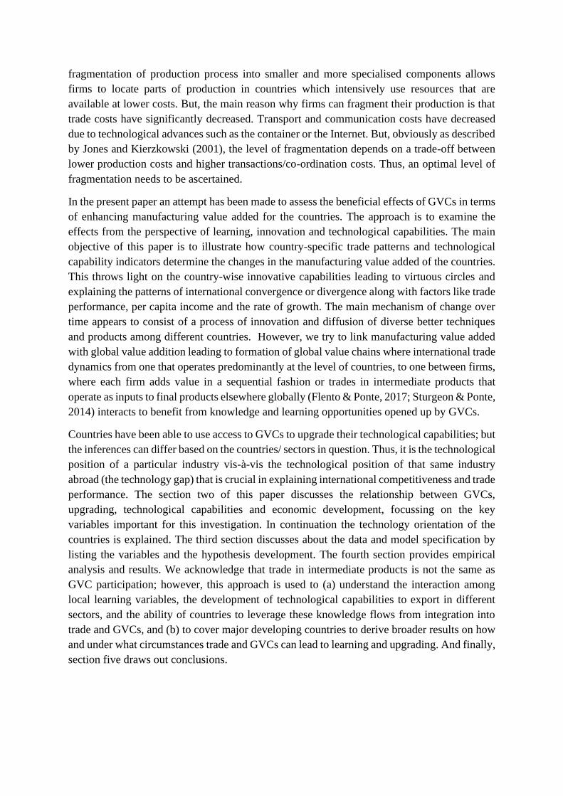
divided into: (a) labour-intensive and resource-intensive low manufactures: textile, leather,
garment and footwear (L1), and (b) low-skill and technology-intensive manufactures: base
metals (L2).
b) Medium-skill technological manufactures
These manufactures are the core of industrial activity in developed economies, and call for
capital intensity and economies of scale, along with sophisticated technological skills that can
be applied to short to medium-term product and process technologies. They imply moderately
high levels of R&D, advanced skills need and lengthy learning periods, and strong backward
and forward linkages, including learning linkages. This category is divided into: medium-skill
and technology-intensive manufactures: medium skill electronics (M2), medium-skill: Parts
and components for electrical and electronic goods (M3), and, medium-skill: Other, excluding
electronics: automobile machinery and engineering goods(M4).
c) High-skill technological manufactures
These manufactures are mostly at the frontier of the field, impute higher levels of R&D
investments, with prime emphasis on design, and new product and process capabilities.
Engaging in such manufacturing requires highly sophisticated technology infrastructures,
specialised technical skills and advanced R&D capabilities with the ability to compete globally.
This category is divided into: high-skill: electronics (excluding parts and components) (H2);
and high-skill: parts and components for electrical and electronic goods other (H3), and high-
skill: other, excluding electronics: automobiles and machinery (H4).
II. Learning variables
a) Patents by residents
Collected from the WDI database, this variable denotes the number of patents by residents,
implying domestic inventions and R&D capacity. This variable is log transformed to control
for skewness.
b) R&D expenditure
Collected from the WDI database, this variable contains R&D expenditure as a percentage of
GDP. This variable has been divided by GDP to control for country-size effects.
c) Scientific publications
Collected from the WDI database, this variable denotes the number of scientific publications
in technical journals. This variable was is transformed to control for skewness.
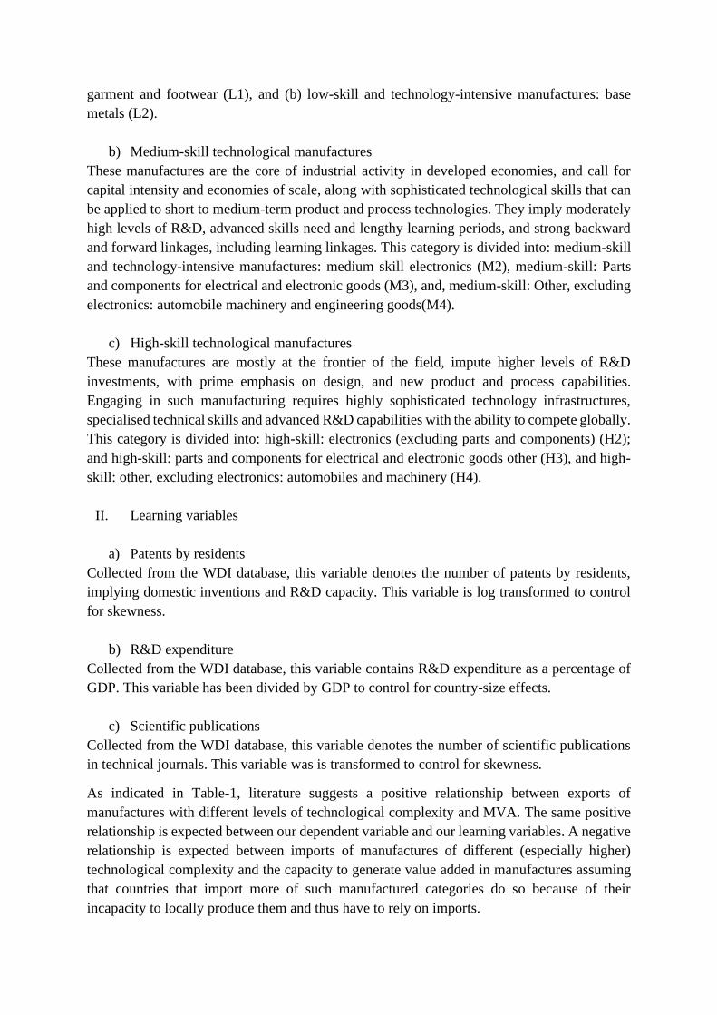
As indicated in Table-1, literature suggests a positive relationship between exports of
manufactures with different levels of technological complexity and MVA. The same positive
relationship is expected between our dependent variable and our learning variables. A negative
relationship is expected between imports of manufactures of different (especially higher)
technological complexity and the capacity to generate value added in manufactures assuming
that countries that import more of such manufactured categories do so because of their
incapacity to locally produce them and thus have to rely on imports.
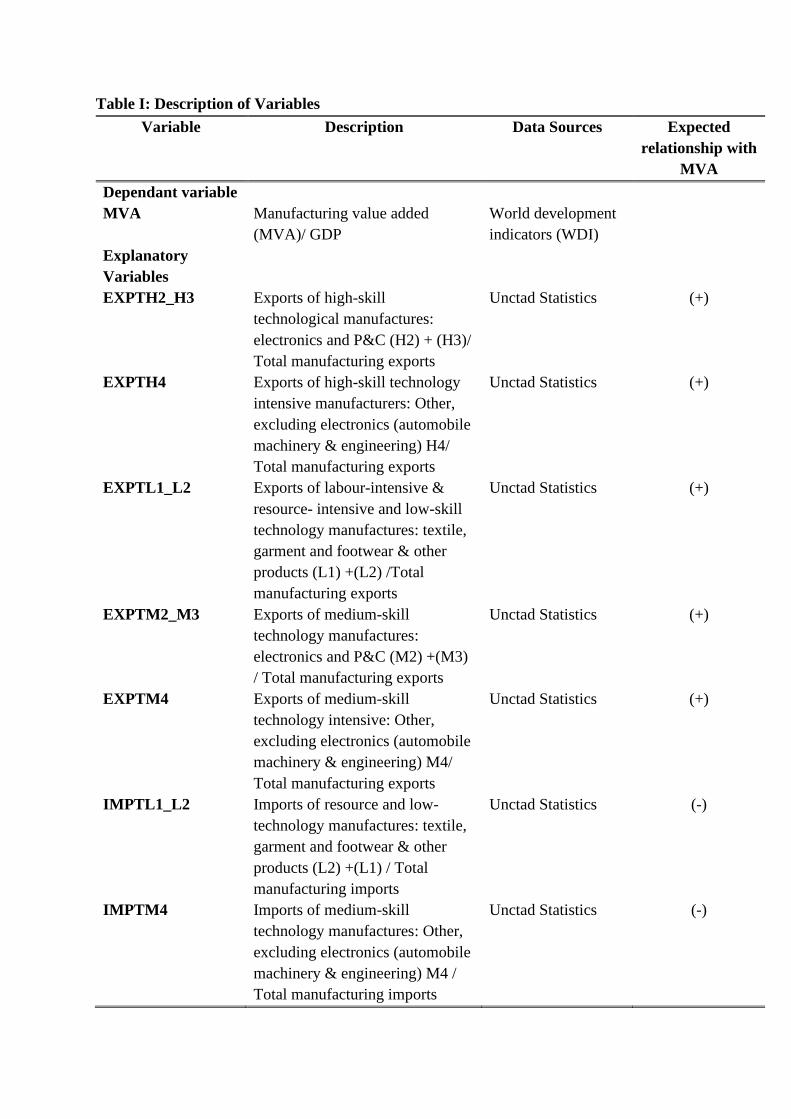
Table I: Description of Variables
Variable Description Data Sources Expected
relationship with
MVA
Dependant variable
MVA Manufacturing value added
(MVA)/ GDP
World development
indicators (WDI)
Explanatory
Variables
EXPTH2_H3 Exports of high-skill
technological manufactures:
electronics and P&C (H2) + (H3)/
Total manufacturing exports
Unctad Statistics (+)
EXPTH4 Exports of high-skill technology
intensive manufacturers: Other,
excluding electronics (automobile
machinery & engineering) H4/
Total manufacturing exports
Unctad Statistics (+)
EXPTL1_L2 Exports of labour-intensive &
resource- intensive and low-skill
technology manufactures: textile,
garment and footwear & other
products (L1) +(L2) /Total
manufacturing exports
Unctad Statistics (+)
EXPTM2_M3 Exports of medium-skill
technology manufactures:
electronics and P&C (M2) +(M3)
/ Total manufacturing exports
Unctad Statistics (+)
EXPTM4 Exports of medium-skill
technology intensive: Other,
excluding electronics (automobile
machinery & engineering) M4/
Total manufacturing exports
Unctad Statistics (+)
IMPTL1_L2 Imports of resource and low-
technology manufactures: textile,
garment and footwear & other
products (L2) +(L1) / Total
manufacturing imports
Unctad Statistics (-)
IMPTM4 Imports of medium-skill
technology manufactures: Other,
excluding electronics (automobile
machinery & engineering) M4 /
Total manufacturing imports
Unctad Statistics (-)

IMPTH4 Imports of high-skill technology
intensive: Other, excluding
electronics (automobile
machinery & engineering) H4/
Total manufacturing imports
Unctad Statistics (-)
PATENTSRES Log of patents by residents World development
indicators (WDI)
(+)
R_DEXP R&D expenditure / GDP World development
indicators (WDI)
(+)
The study takes into account a dataset of 14 developing countries from UNCTAD list of
developing countries, considered as cross sections. These countries provide a comparative
perspective to India when it comes to manufacturing sector for all these variables and panel
data regression is run for nineteen years, from 2000 to 2018 to draw conclusions on how and
which learning variables impact the technological export categories in which countries export
over time.
The data set comprises of time and spatial components therefore giving rise to panel data
structure. Based on the above theoretical discussion, the model can be written as:
MVAit = β0 + β1 EXPH1_H2it + β2 EXPH4it + β3 EXPL1_L2it + β4 EXPM2_M3it + β5 EXPM4it
+ β6 IMPH4it + β7 IMPL1_L2it + β8 IMPM4it + β9 R_DEXPit + β10 PATENTSRESit + Ɛit ……...
(Equation 1),
Considering the description of the variables from table-1, MVAit is predicted or expected value
of manufacturing value added for country i in year t as a percentage of GDP. β0 is the value of
MVAit when all independent variables are equal to zero in year t. β1it to β5it are the estimated
regression coefficients for export variables with expected positive signs for all the years.
EXPH1_H2, EXPH4, EXPL1_L2, EXPM2_M3it and EXPM4it are the values of manufacturing
export variables with different levels of technological intensity for country i in year t as a
percentage of total manufacturing exports. Β6it to β8it are the estimated regression coefficients
for import variables with expected negative signs for all the years. IMPH4it, IMPL1_L2it and
IMPM4it are the values of manufacturing import variables with different levels of technological
intensity country i in year t as a percentage of total manufacturing imports. R_DEXPit and
PATENTSRESit are the values of learning variables for country i in year t with Β9it and β10it as
regression coefficients with expected positive signs for all years and countries. And Ɛit are the
errors of the regression equation.
During the regression, several data points are located far outside the mean of the group. To
identify these data points, which are observations with large residuals that affect the dependent-
variable value in an unusual form, we first calculate the leverage by standardising the predictor
variable to a mean equal to zero and a standard deviation equal to one. The transformation of
a row score X is then done by using the following formula:
Xstandardised = (X – μ) / σ ……... (Equation 2),

where μ = the mean and σ = the standard deviation.
Given that our variables are related to each other, it is important to test for multicollinearity. A
Variation Inflation Factor (VIF) test is used to quantify the extent to which the variance is
inflated and that helps us detect multicollinearity. VIFk helps to estimate the inflation factor for
the variance of estimated coefficient bk. That is to say,
VIFk = 1/1 − 𝑅𝑘2……... (Equation 3),
where 𝑅𝑘2 is the R2 value obtained by regressing the kth predictor on the remaining predictors.
We accept that if the VIF is larger than 8 it implies severe multicollinearity issues and thus it
is removed from the analysis.
IV. Methodology, empirical results and discussions
1. Descriptive statistics and correlations
The model being multivariable, it is deliberated to take standardised version of the variables as
it puts variables on the same scale and minimises correlation among them while aiding in
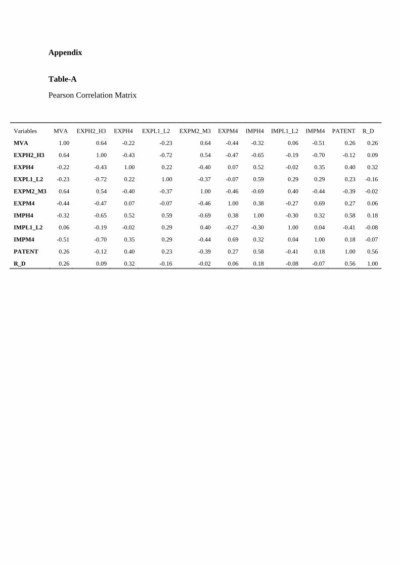
estimating the variables. Table-A of appendix section, presents the Pearson product-moment
correlation coefficient, which measures the direction and strength of the relationships between
any two continuous variables. Since we are only interested in the correlation between the
explanatory variables and dependent variable, the correlations among explanatory variables are
not discussed here. The signs of the Pearson correlation coefficients, r, with respect to
dependent variable (value added in manufacturing) are positive, indicating a positive
correlation among these variables, except for export and import of H4, export and import of
M4, and export of L1+L2 which present negative correlations. This indicates that higher values
of these variables are associated with lower levels of value added in manufacturing. Higher
values amongst the rest of the variables are associated with greater levels of value added in
manufacturing. This holds for all the years under consideration from 2000 to 2018.
Table-B shows a large correlation2 between the dependent variable and exports of H2+H3 and
exports of M2+M3. A moderate correlation3 between the dependent variable and exports of
M4 is also observed, however the rest of the variables present a smaller level of correlation4
with value added in manufacturing. Expecting relationships between the variables used in the
regression, the multicollinearity test is run with all the variables in our sample before
proceeding with the analysis. The results indicate high levels of multicollinearity among certain
variables which would affect the results of the regression if included. This is the case
particularly with imports of high skill and technology-intensive manufactures (H2+H3) which
is highly correlated with exports of resource-intensive and low-skill and technology-intensive
(L1+L2), exports of high skill and technology-intensive manufactures (H2+H3) and imports of
medium-skill and technology-intensive manufactures (M2+M3). Even variable publications is
highly correlated with patent and import of high-skill and technology intensive imports (H4).
2 | r | > 0.5 3 0.3 < | r | < 0.5 4 0.1<||r|<0.3
Therefore, the variables; import of H2+H3, import of M2+M3 and scientific publications are
removed from the analysis.
2. Unit root test
Testing for stationarity in panel data models is also per se a matter of interest but it seems fairly
intuitive that, within the general class of models where heterogeneity is restricted to an
individual fixed effect, the times series behaviour of an individual variable should often be well
approximated either as an autoregressive process with a small positive coefficient and large
fixed effects or as an autoregressive process with a near-unit root and almost negligible
individual fixed effects. Both alternatives can be nested in a single model and trying to assess
the properties of the available tests in a realistic setting is therefore of practical importance,
Hall-Mairesse (2002).
Since panel data has time-series element, unit root test is required for testing stationarity in
panel data as results will be spurious if data doesn't satisfy the stationarity assumption implicit
in most tests. Tests such as Levin-Lin-Chu test which is considered to be the ADF equivalent
for panel data can be used. Recently, there has been a heightened development of panel-based
unit root tests (Hadri, 1999; Breitung, 2000; Choi, 2001; Levin et al. 2002; Im et al. 2003;
Breitung and Das, 2005). These studies have shown that the panel unit root tests are less likely
to be subject to Type II error and as such are more powerful than tests based on times series
data. By running a balanced panel data, panel unit root test is performed.
Due to the nature of the dataset, Fisher-type Augment Dickey Fuller (ADF) tests as presented
by Choi (2001) is employed. The ADF specification equation can be written as:
Δyit = ρi yi, t-1 + z’it ɣi + vit
where i=1…...N, t=1……. T, and vit denote the stationary error term of the i th member in
period t, respectively. yit refers to the variable being tested, z’it represents with panel-specific
means, time trends, or nothing depending on the options specified. If zit=1, then z’it ɣi will
denote fixed-effects. On the other hand, a trend scenario can be specified where z’it= (1, t) such
that z’it ɣi represents fixed-effects and linear time trends.
In testing for panel-data unit roots, Fisher-type tests conduct the unit-root tests for each panel
individually and then combine the p-values from these tests to produce an overall test (an
approach used mostly in meta-analysis). Note that in this context, a unit-root test on each of
our panel units i is separately performed and then their combined p-values are used to construct
a Fisher-type test to investigate whether or not the series exhibit a unit-root. The null hypothesis
in this case is HO: ρi=1 for all i versus the alternative hypothesis of Ha: ρi<0 for some i.
From the Fisher-Type ADF unit root tests the results are presented in Table-3. As can be seen,
the variables are stationary at level.

Table II: Panel unit root test
Panel
Unit
Root
Test
MVA EXPH2_H3 EXPH4 EXPL1_L2 EXPM2_M3 EXPM4 IMPH4 IMPL1_L2 IMPM4 PATENT R_D
ADF -
Fisher
Chi-
square
0.01* 0.00** 0.02* 0.00** 0.01* 0.00** 0.03* 0.00** 0.02* 0.00** 0.01*
∗∗, ∗∗∗ Significance at the 1% & 5% level
Thus, the variables being stationary at level, the data is checked for fixed or random effects.
3. Panel data modelling
Considering equation 4 as the base, after cleaning the data and checking its quality and getting
a strong impression of presence of fixed and/or random effects, the Hausman specification test
(Hausman, 1978) is used. If the null hypothesis that the individual effects are uncorrelated with
the other regressors is not rejected, a random effect model is favoured over its fixed counterpart.
But, in our case the null hypothesis is rejected and the model favours fixed effects model.
The cross-sectional dependence is one of the most important diagnostics that a researcher
should investigate before performing a panel data analysis. In this context, the Breusch and
Pagan (1980) LM test and Pesaran (2004) CD test, were utilized. The problem of cross-
sectional dependence arises if n individuals in sample are no longer independently drawn
observations but affect each other’s outcomes. For example, this can result from the fact that
we look at a set of neighbouring countries, which are usually highly interconnected. Findings
in Table 4 illustrate that the null of “no cross-sectional dependence” is rejected even at 1%
level of significance. Therefore, there is a need to proceed with tests and estimation techniques
that can take account of cross-sectional dependence.
Table III: Residual Cross-Section Dependence Test before using weights
Null hypothesis: No cross-section dependence (correlation) in
residuals
Test Statistic d.f. Prob.
Breusch-Pagan LM 391.7554 91 0
Pesaran CD -2.31639 0.0105
The most appropriate and classic model of error cross-sectional dependence in econometrics is
the Seemingly Unrelated Regressions (SUR) approach, due to Zellner (1962). The SUR
approach leads to a feasible GLS estimator, in which OLS is used at first-stage for each

individual-specific equation to obtain consistent estimates of the parameters. Using cross-
section SUR weights, EViews estimates a feasible GLS specification correcting for
heteroskedasticity and contemporaneous correlation. Thus, the findings from table-5 suggests
that the null hypothesis can’t be rejected at even at 1% level of significance.
Table IV: Residual Cross-Section Dependence Test after using weights
Null hypothesis: No cross-section dependence
(correlation) in weighted residuals
Test Statistic d.f. Prob.
Breusch-Pagan LM 10.78383 91 1
Pesaran CD -0.763476
0.4452
So, now least square dummy variable (LSDV) is applied to capture the fixed effects in the
model. It provides a good way to understand fixed effects. The country effects taken as cross
sections and sectoral effects taken as explanatory variables on manufacturing value added
considered as dependant variable are checked.
The standard fixed effects model:
Yit = αi + X’itβ + Ɛit, ……... (Equation 7),
With t = 1……T time periods and i = 1……. N cross-sectional units.
• The αi contain the omitted variables, constant over time, for every unit i.
• The αi are called the fixed effects, and induce unobserved heterogeneity in the model.
• The X’it are the observed part of the heterogeneity. The Ɛit contain the remaining omitted
variables.
Here, testing for unobserved heterogeneity is done through dummy variables.
Rewriting the model as
Yit = α1𝐷𝑖1 +……………...+an𝐷𝑖
1 + X’itβ + Ɛit, (Equation 8),
With 𝐷𝑖𝑗 = 1 if i = j and zero if i ≠ j
However, the core difference between fixed and/or random effect model lies in the role of
dummy variables as a parameter estimate of a dummy variable belongs to intercept in a fixed
effect model and to an error component in a random effect model. A fixed group effect model
examines individual differences in intercepts, assuming the same slopes and constant variance
across individual (group and entity), (Baltagi, 2005; Bourbonnais, 2009).
Taking the LSDV model where dummy variables for the countries are considered as cross
sections, the further checking if these dummies are jointly significantly different from zero
with wald statistics is carried out (results are presented in table-7). The analysis considers 14
developing countries namely, Brazil (DB), China(DC), South Korea(DK), Russia(DR),

India(DI), Mexico(DX), Indonesia(DN), Philippines(DP), Singapore(DS), Thailand(DT),
Malaysia(DM), Vietnam(DV), Turkey(DY) and South Africa(DA) and within brackets are
their respective dummy names used in the panel regression with information from year 2000
to 2018.
Table V: Panel data analysis
Dependent Variable: MVA
Method: Panel EGLS (Cross-section SUR)
Sample: 2000 2018
Periods included: 19
Cross-sections included: 14
Total panel (balanced) observations: 266
Linear estimation after one-step weighting matrix
Variable Coefficient Std. Error t-Statistic Prob.
EXPH2_H3 1.041620 0.022904 45.47682 0.0000*
EXPH4 0.162856 0.007097 22.94622 0.0000*
EXPL1_L2 0.565015 0.020231 27.92775 0.0000*
EXPM2_M3 0.150187 0.015149 9.913911 0.0000*
EXPM4 0.367874 0.011838 31.07654 0.0000*
IMPH4 0.019854 0.002879 6.896926 0.0000*
IMPL1_L2 0.131041 0.005978 21.91933 0.0000*
IMPM4 -0.018772 0.002914 -6.440997 0.0000*
R_D -0.037771 0.002889 -13.07325 0.0000*
PATENT 0.328974 0.051991 6.327545 0.0000*
DA -0.088682 0.003974 -22.31699 0.0000*
DB -0.468930 0.018847 -24.88142 0.0000*
DC 0.249109 0.021628 11.51815 0.0000*
DK 0.087813 0.006909 12.71036 0.0000*
DM -0.004057 0.006973 -0.581793 0.5612
DN -0.016317 0.007810 -2.089309 0.0377**
DP -0.116982 0.005883 -19.88313 0.0000*
DR -0.060822 0.005860 -10.37849 0.0000*
DS -0.015409 0.005015 -3.072694 0.0024*
DT 0.019475 0.009156 2.126966 0.0344**
DV -0.139864 0.008608 -16.24736 0.0000*
DX -0.100802 0.004899 -20.57692 0.0000*
DY -0.102921 0.004291 -23.98519 0.0000*
C 0.003648 0.004059 0.898783 0.3697
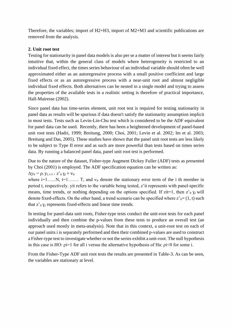
Weighted Statistics
Root MSE 0.947189 R-squared 0.999368
Mean dependent var -57.59948 Adjusted R-squared 0.999308
S.D. dependent var 99.33502 S.E. of regression 0.993047
Sum squared resid 238.6464 F-statistic 16647.71
Durbin-Watson stat 1.717784 Prob(F-statistic) 0.000000
Unweighted Statistics
R-squared 0.932682 Mean dependent var -0.290902
Sum squared resid 1.082225 Durbin-Watson stat 0.330647
The findings suggest a synergistic relationship between the opportunities for upgrading
presented by GVCs and local technological capabilities being developed. We find that in the
case of those countries that use trade and GVC participation to develop a diversified
technological base, their increased ability to generate MVA and outperform is parallelly shaped
by a number of in-country institutional factors that help them to continuously learn and develop
technological capabilities that benefit them. From table-6 above, after correcting for serial
correlation by using SUR weights, the LSDV fixed effects is performed. The weighted statistics
R2 has improved along with Durbin-Watson value. The impact of explanatory variables on
MVA has come out to be significant, but the signs of the variables throw some light on their
relationship. The import category of medium technology involving automobile and machinery
engineering products (M4) shows a negative relationship with value added in manufacturing
for all countries in our sample. This indicates that developing countries importing this type of
products demonstrated lower MVA in a significant level over time, suggesting that it might be
both the result of, and leading to, lower learning and capabilities formation in the local
economies. These results are supported by other studies (see Morrison et al., 2008, WIPR,
2017, Gibbon & Ponte, 2005), that suggest that as countries acquire more and more ready
products, particularly those products with high content of engineering skills and technology,
they do not present significant learning and technological upgrading possibilities and also
eliminate several local firms actively engaged in producing such products, thereby inducing
deskilling.
The analysis shows that from all the different learning variables, only patents by residents had
a significant and positive relationship with value added in manufacturing for all the countries
and years. However, the surprise comes from sign of expenditure on R&D, this only indicates
that developing countries could rather import R&D intensive technologies to increase their
manufacturing value addition and technological capabilities further. This aspect particularly
hints at reaping the benefits from spill overs and through learning. The import of sophisticated
goods (be it capital or other intermediate products) and inward foreign direct investment (FDI)
flows leading to technological spillovers/dissemination have benefited different manufacturing
sectors in many countries. The various sources from which technological learning can take
place, correspond to multiple learning interaction effects taking place (1) within the firm
(learning by doing), (2) between the firm and the environment (learning by exporting and a
firm’s absorptive capacity to acquire intra- and inter-industry learning spillovers) where
learning from exporting has been found to be more pronounced for firms that belong to an

industry which has high exposure to foreign firms (Greenaway and Kneller, 2008), are younger,
or have a greater exposure to export markets (Kraay, 1999; Castellani, 2002). And, lastly (3)
external to the firm (intra- and inter-industrial learning spillovers mediated by institutions).
Finally, we check for individual country effects and if they are significantly different then there
is unobserved heterogeneity. Checking from the Wald statistics (Wald test of coefficient
restrictions) from the table-7, we reject the null hypothesis at 1% level of significance in favour
of alternative hypothesis that the dummy variables are significantly different from zero. By
adding dummy for each country, we are estimating pure effect of explanatory variables on
MVA. Thus, each dummy is absorbing the effects particular to each country. Taking the base
category as India, we try and compare each country with it. Apart from China, South Korea
and Thailand, all other countries have MVA less than India. The average MVA difference
among countries can be seen through their coefficients, signs and significance. Sorting these
countries from highest coefficient to lowest, China, South Korea, Thailand, India and Malaysia
are the top five countries with their underlying characteristics that are informative about MVA
apart from the variables considered for each country impacting MVA. These country effects
highlight the differences in policy orientation, institutional mechanisms and the ability to
technologically converge with superior countries so as to gain in the maximum possible way
from the existing comparative advantage.
Table IV: Wald test result
Test Statistic Value Df Probability
F-statistic 460.9983 (14, 228) 0
Chi-square 6453.977 14 0
Null Hypothesis:
C(11)=C(12)=C(13)=C(14)=C(15)=C(16)=
C(17)=C(18)=C(19)=C(20)=C(21)=C(22)=C(23)=C(24)=0
V. Conclusion
The manufacturing sector’s role in supporting economic growth and development has been
underpinned by a range of characteristics with the potential for spill overs and dynamic
productivity gains: scale, tradability, innovation, learning by doing, and job creation. Relying
on manufacturing exports has been the mode of escape from under-development for many East
Asian Countries. Starting with relatively low-skilled manufacturing, mainly textiles and
clothing. These countries then diversified into more sophisticated manufacturing involving
high tech-low value items like electronics and automobiles-- an idea behind technological
catch-up that earned the reputation of quality, standard, and value for price in the international
market.
This relationship between technology and trade for developing countries still favors low
technology industries. However, owing to the growing trade fragmentation process in the last
decades, exports of high-tech electronic products is mostly done by low-income countries that

instead of introducing innovation to product development, the manufacturing process is
confined mainly to assemble and test final products. But, in the case of India, (Athukorala and
Menon (2010)), show that India is a minor player in global production networks and vertical
specialisation-based trade. The trend and pattern of overall trade of different technology-
intensive categories for different countries show that India, China, Turkey and Vietnam are the
exceptions with higher AAGR in comparison to other countries in every technology-intensive
category. Also, having maximum structural changes in export of resource intensive category
(measured by Lawrence index) which majorly comprises of textile and apparels, these countries
show that their exports still being concentrated in this category, are now diversifying more in
the MSI and HSI categories (captured by trade margins). This presents the potential
opportunities provided by participating in GVCs and reaping the benefits of integration with
world production process.
The empirical analysis also points to the same conclusion where both the EXPL1_L2 and
EXPH2_H3 come out significant with positive signs and also with higher coefficient values
for all developing countries from 2000 to 2018 associated with MVA. This stresses in
specialising by countries according to their comparative advantages and integrating with the
production of network products. Also, the developing countries display a greater local
manufacturing value added in the automobile sector captured by EXPM4. Assessing the
developments in conjunction with technological capability variables, only patents of residents
was a significant factor leading to increase in manufacturing value added.
Among all the countries, China’s exceeding performance can be explained by its consistent
investments into learning, export capabilities and export surplus leading to its current global
position in trade. Here even India, Malaysia, Thailand and South Korea can be pitted against
each other in terms of country characteristics which are not fixed but innate to a manufacturing
subsector, but vary across countries and over time. Finally, our analysis focuses on the critical
role of national learning variables in accounting for how countries trade and participate in
GVCs. We conclude that upgrading in and through trade and GVCs can be understood at best
with the combined association of these phenomenon with technological capabilities.
References
• Altenburg, T. (2006). Governance patterns in value chains and their development impact. The
European Journal of Development Research, 18(4), 498-521.
• Athukorala, P. C., & Menon, J. (2010). Global Production Sharing, Trade Patterns and
Determinants of Trade Flows (No. 2010-06).
• Baffes, J. (2006). Restructuring Uganda’s Coffee Industry: Why Going Back to the Basics
Matters. World Bank Policy Research Working Paper. The World Bank. Washington, D.C.
• Baldwin, R., & Lopez‐Gonzalez, J. (2015). Supply‐chain trade: A portrait of global patterns
and several testable hypotheses. The World Economy, 38(11), 1682-1721.
• Baltagi, B. H. (2005). Econometric Analysis of Panel Data, John Wiley&Sons Ltd. West
Sussex, England.
• Barba Navaretti, G., & Venables, A. J. (2004). Host country effects: conceptual framework and
the evidence. Multinational Firms in the World Economy. Princeton University Press, Princeton
and Oxford, 151-182.
• Bazan, L., & Navas-Aleman, L. (2004). The Underground Revolution in the Sinos Valley: A
comparison of Upgrading in global and national value chain. In H. Schmitz (Ed.), Local
Entreprises in the Global Economy: Edward Elgar Publishing.
• Bell, M., & Albu, M. (1999). Knowledge Systems and Technological Dynamism in Industrial
Clusters in Developing Countries. World Development, 27(9), 1715-1734.
• Bell, M., & Pavitt, K. (1992). Accumulating technological capability in developing countries.
The World Bank Economic Review, 6(suppl_1), 257-281.
• Bell, M., & Pavitt, K. (1995). The development of technological capabilities. Trade, technology
and international competitiveness, 22(4831), 69-101.
• Breitung, J. (2000) The Local Power of Some Unit Root Tests for Panel Data. Advances in
Econometrics
• Breitung, J., & Das, S. (2005). Panel unit root tests under cross‐sectional dependence. Statistica
Neerlandica, 59(4), 414-433.
• Breschi, S., Malerba, F., & Orsenigo, L. (2000). Technological regimes and Schumpeterian
patterns of innovation. The economic journal, 110(463), 388-410.
• Breusch, T. S., & Pagan, A. R. (1980). The Lagrange multiplier test and its applications to
model specification in econometrics. The review of economic studies, 47(1), 239-253.
• Cassen, R., & Lall, S. (1996). Lessons of East Asian development. Journal of the Japanese and
International Economies, 10(3), 326-334.
• Castellani, D. (2002). Export behavior and productivity growth: Evidence from Italian
manufacturing firms. Weltwirtschaftliches Archiv, 138(4), 605-628.
• Choi, In. (2001). Unit Root Tests for Panel Data. Journal of International Money and Finance.
20. 249-272.
• Cohen, W. M., & Levinthal, D. A. (1990). Absorptive capacity: A new perspective on learning
and innovation. Administrative science quarterly, 128-152.
• Dahlman, C. J., Ross-Larson, B., & Westphal, L. E. (1987). Managing technological
development: lessons from the newly industrializing countries. World development, 15(6), 759-
775.
• De Marchi, V., Giuliani, E., & Rabelloti, R. (2015). Local innovation and global value chains
in developing countries. UNU-MERIT Working Paper Series. UNU-MERIT. Maastricht
• De Marchi, V., Giuliani, E., & Rabellotti, R. (2018). Do global value chains offer developing
countries learning and innovation opportunities? The European Journal of Development
Research, 30(3), 389-407.
• Escaith, H, N Lindenberg, and S Miroudot (2010) “International Supply Chains and Trade
Elasticity in Times of Global Crisis,” WTO Staff Working Paper ERSD201008
• Estevadeordal, A., Blyde, J., Harris, J., & Volpe, C. (2013). Global Value Chains and Rules of
Origin. E15 initiative. Strengthening the Global Trade System. International Centre for Trade
and Sustainable Development (ICTSD) and World Economic Forum
• Evenson, R. E., & Westphal, L. E. (1995). Technological change and technology strategy.
Handbook of development economics, 3, 2209-2299.
• Feenstra, R. C., & Hamilton, G. G. (2006). Emergent Economies, Divergent Paths: Economic
Organization and International Trade in South Korea and Taiwan (Vol. 29).
• Flento, D., & Ponte, S. (2017). Least-Developed Countries in a World of Global Value Chains:
Are WTO Trade Negotiations Helping? World Development, 94, 366-374.
• Gereffi, G. (1994). 1994: The organization of buyer-driven global commodity chains: how US
retailers shape overseas production networks. In Gereffi, G. and Korzeniewicz, M., editors,
Commodity chains and global capitalism, Westport, CT: Greenwood Press, 95-122.
• Gereffi, G. (1999). International trade and industrial upgrading in the apparel commodity chain.
Journal of International Economics, 48(1), 37-70.
• Gereffi, G., & Kaplinsky, R. (2001). Introduction: Globalisation, value chains and
development. IDS bulletin, 32(3), 1-8.
• Gibbon, P., & Ponte, S. (2005). Trading down: Africa, Value Chains, And The Global
Economy. Philadelphia: Temple University Press.
• Greenaway, D., & Kneller, R. (2008). Exporting, productivity and agglomeration. European
economic review, 52(5), 919-939.
• Hadri, K. (1999). Testing the null hypothesis of stationarity against the alternative of a unit root
in panel data with serially correlated errors (No. 1999_05).
• Hall, B. H., & Mairesse, J. (2009). Measuring corporate R&D returns. Presentation to the
Knowledge for Growth Expert Group, Directorate General for Research, European
Commission, Brussels, January.
• Hummels, D., Ishii, J., & Yi, K. M. (2001). The nature and growth of vertical specialization in
world trade. Journal of international Economics, 54(1), 75-96.
• Humphrey, J., & Schmitz*, H. (2001). Governance in global value chains. IDS bulletin, 32(3),
19-29.
• Humphrey, J., & Schmitz, H. (2000). Governance and Upgrading. Linking Industrial Cluster
and Global Value Chain Research. Brighton: Institute of Development Studies.
• Im, K. S., Pesaran, M. H., & Shin, Y. (2003). Testing for unit roots in heterogeneous panels.
Journal of econometrics, 115(1), 53-74.
• Jones, R. W., & Kierzkowski, H. (2001). Horizontal aspects of vertical fragmentation. In Global
production and trade in East Asia (pp. 33-51). Springer, Boston, MA.
• Kaplinsky, R. (2000). Globalisation and unequalisation: what can be learned from value chain
analysis? Journal of development studies, 37(2), 117-146.
• Katz, J. M. (Ed.). (1987). Technology generation in Latin American manufacturing industries.
Springer.
• Kraay, A. (1999). Exports and economic performance: Evidence from a panel of Chinese
enterprises. Revue d’Economie du Developpement, 1(2), 183-207.
• Lall, S. (1987). Learning to industrialize: the acquisition of technological capability by India.
Springer.
• Lall, S. (1992). Technological capabilities and industrialization. World development, 20(2),
165-186.
• Lall, S. (2001). Competitiveness, technology and skills. Books.
• Lall, S. (2004). Reinventing Industrial Strategy: The Role of Government Policy in Building
Industrial Competitiveness. G-24 Discussion Paper Series. UNCTAD. New York and Geneva.
• Lee, K. (2013). Schumpeterian Analysis of Economic Catch-up: Knowledge, Path-creation and
Middle-Income Trap. Cambridge, Mass: Cambridge University Press.
• Levin, A., Lin, C. F., & Chu, C. S. J. (2002). Unit root tests in panel data: asymptotic and finite-
sample properties. Journal of econometrics, 108(1), 1-24.
• Markusen, J. R., & Venables, A. J. (1999). Foreign direct investment as a catalyst for industrial
development. European economic review, 43(2), 335-356.
• Morrison, A., Pietrobelli, C., & Rabellotti, R. (2008). Global value chains and technological
capabilities: a framework to study learning and innovation in developing countries. Oxford
development studies, 36(1), 39-58.
• Nelson, R. R., & Winter, S. G. (1982). The Schumpeterian tradeoff revisited. The American
Economic Review, 72(1), 114-132.
• Pesaran, M. H. (2004). General diagnostic tests for cross section dependence in panels.
• Pietrobelli, C. (1997). On the theory of technological capabilities and developing countries'
dynamic comparative advantage in manufactures. Rivista Internazionale di Scienze
Economiche e Commerciali, 44, 313-338.
• Pietrobelli, C. (1998). Industry, Competitiveness and Technological Capabilities in Chile: A
New Tiger from Latin America? Springer.
• Pietrobelli, C., & Rabelloti, R. (2011). Global Value Chains Meet Innovation Systems: Are
There Learning Opportunities for Developing Countries? World Development, 39(7), 1261-
1269.
• Ponte, S. (2002). The 'Latte Revolution'? Regulation, Markets and Consumption in the Global
Coffee Chain. World Development, 30(7), 1099-1122.
• Sturgeon, T., & Ponte, S. (2014). Explaining governance in global value chains: A modular
theory-building effort. Review of International Political Economy, 21(1), 195-223.
• Vallejo, B. (2010). Learning and Innovation under Changing Market Conditions. The Auto
Parts Industry in Mexico. (Ph.D. in the Economics and Policy Studies of Technical Change),
Maastricht University, Maastricht, The Netherlands.
• "World Intellectual Property Report 2017: Intangible Capital in Global Value Chains" (WIPR
2017), WIPO.
• Zellner, A. (1962). An efficient method of estimating seemingly unrelated regressions and tests
for aggregation bias. Journal of the American statistical Association, 57(298), 348-368.
Appendix
Table-A
Pearson Correlation Matrix
Variables MVA EXPH2_H3 EXPH4 EXPL1_L2 EXPM2_M3 EXPM4 IMPH4 IMPL1_L2 IMPM4 PATENT R_D
MVA 1.00 0.64 -0.22 -0.23 0.64 -0.44 -0.32 0.06 -0.51 0.26 0.26
EXPH2_H3 0.64 1.00 -0.43 -0.72 0.54 -0.47 -0.65 -0.19 -0.70 -0.12 0.09
EXPH4 -0.22 -0.43 1.00 0.22 -0.40 0.07 0.52 -0.02 0.35 0.40 0.32
EXPL1_L2 -0.23 -0.72 0.22 1.00 -0.37 -0.07 0.59 0.29 0.29 0.23 -0.16
EXPM2_M3 0.64 0.54 -0.40 -0.37 1.00 -0.46 -0.69 0.40 -0.44 -0.39 -0.02
EXPM4 -0.44 -0.47 0.07 -0.07 -0.46 1.00 0.38 -0.27 0.69 0.27 0.06
IMPH4 -0.32 -0.65 0.52 0.59 -0.69 0.38 1.00 -0.30 0.32 0.58 0.18
IMPL1_L2 0.06 -0.19 -0.02 0.29 0.40 -0.27 -0.30 1.00 0.04 -0.41 -0.08
IMPM4 -0.51 -0.70 0.35 0.29 -0.44 0.69 0.32 0.04 1.00 0.18 -0.07
PATENT 0.26 -0.12 0.40 0.23 -0.39 0.27 0.58 -0.41 0.18 1.00 0.56
R_D 0.26 0.09 0.32 -0.16 -0.02 0.06 0.18 -0.08 -0.07 0.56 1.00