asia and pacific commission on agricultural · pdf fileasia and pacific commission on...
TRANSCRIPT

RAP/APCAS/14/13.2
1
Asia and Pacific Commission on
Agricultural Statistics
Twenty-fifth Session
Vientiane, Lao PDR, 18-21 February 2014
Agenda Item 13
Recent advancements in Agricultural Economic Statistics – Price and Investment domains
Contributed by: FAO Statistics Division
1. Price Statistics - Introduction
The 2007 food price crisis, with its implications for food security, underlined the
importance in improving the monitoring of agriculture and food price transmissions across the
value-chain. Though FAO is the main provider of internationally comparable data on agricultural
producer prices, the need to better monitor agriculture food price transmissions requires it expand
its previous work on agricultural prices in four key directions. These include: 1) improve the
coverage, frequency and timeliness of price statistics to measure farm to fork food and agriculture
prices; 2) improve dissemination and awareness of FAO price data by accompanying new data
releases with statistical analysis; 3) develop, evaluate and disseminate a new set of derived
indicators to better capture and monitor price dynamics, transmission and volatility; and 4)
consolidate and disseminate these price datasets and indicators in price profiles to provide quick
and easy access to price information for different geographic groupings.
This paper presents and describes the data currently collected on agricultural and food
prices, the new dissemination strategy, and new indicators and price profiles currently under
development. It also solicits discussion and advise from APCAS member countries on how to
January 2014 E

RAP/APCAS/14/13.2
2
improve underlying country-level data, and how FAO can best provide relevant and timely price
information and analytical products to member countries.
2. Setting the context – Key Uses of Price Statistics
Agricultural prices influence public and private decisions related to the type and volume of
agricultural policy and production, be it made by national governments, farmers and other agri-
businesses, or international organizations.
National governments use agriculture price data to develop, monitor and evaluate food price
subsidies as well as other agriculture support policies; to identify intra-country and international
comparative advantage in the type and composition of agricultural production; and to identify
population groups at risk as a result of price volatility or disruptions in the agriculture value-
chain. Price data is also used to estimate the value of agricultural output, intermediate inputs, and
agricultural value added, in both real and nominal terms, which in turn provides data essential for
productivity analysis.
Farmers and agri-businesses use price information to inform decisions about agricultural
production and composition; use and purchase of intermediate inputs, including feed, fertilizers,
labour and machinery; and borrowing, farm management and investment decisions.
International organizations use agricultural price data for similar analytical and policy
purposes as national governments. For their purposes, standardization in the methodologies
behind data collection helps ensure that cross-country comparisons are able to identify differences
in policies, environment, production, and productivity, and are not an artefact of differences in
definitions or the manner in which data are collected, estimated or disseminated1.
3. Current and planned work on Prices
a. Producer prices
FAO provides annual country-level data on producer prices for primary crop and livestock
products dating back to 19912; monthly producer prices beginning January 2010; and annual
producer price indexes (PPIs) for 1999 to 2011. FAO’s producer price database has the largest
coverage of producer prices in the world, with a coverage of approximately 150 countries and
about 200 commodities, representing roughly 97 percent of the world’s value of agricultural
production at 2004-2006 international dollar prices. Absolute producer prices are available in
local currency, standard local currency and US dollars, with continuous efforts made to expand
country coverage and improve data quality.
1 More details available in “Farm and input prices: collection and compilation”, FAO, 1980.
2 An older database (“Producer Price Archive”), with historical data from 1966 to 1990 is also available on
FAOSTAT. This database is not anymore maintained and updated.

RAP/APCAS/14/13.2
3
Producer prices, collected annually through a price questionnaire, refer to prices received by
farmers, known as “farm gate” or first-point-of-sale prices, when farmers participate in their
capacity as sellers of their own products. To maximize international comparability, countries are
requested to remain as close as possible to this concept. However, due to differences in data
collection infrastructure and capacity, countries do vary from this concept by collecting, instead,
wholesale or local market prices. While these may be good proxies of farm-gate prices when the
marketing chain is very limited, they tend to be poorer proxies in economies where transport and
commercial margins constitute a significant share of the final product price. At the far extreme,
some countries report retail prices, which are typically very poor proxies for producer prices.
As FAO begins work on Cost of Production statistics and the Economic Accounts of
Agriculture (EAA), the proximity of price data to the producer price concept will become
increasingly important. Producer prices are an essential input into both statistical activities, and
both are used by policy makers to evaluate comparative advantage within their country and
against major competitors, in identifying productivity enhancing inputs, and in establishing
agricultural support policies.
b. Consumer prices, and regional and global price indexes
To extend statistical coverage of agricultural price statistics and better investigate price
transmission, in 2011 FAO began to disseminate country-level data on Consumer Price Indices
(CPI), using data compiled by the International Labour Organization (ILO), for the food and all-
items index, for about 140 countries3. Since August 2013, FAO also began publishing regional
and global food CPIs4. These indicators, compiled quarterly for FAO regions, add to the set of
regional indices from other data domains, such as production and trade. In the near future, these
set will be further enhanced with the addition of regional and global PPIs.
Such aggregate indicators help identify common trends across regions as well as country-
level differences, and the drivers behind both. They can also serve to identify leading indicators
of phenomenon such as food price hikes and food insecurity. For example, a comparison of the
historical trend in the FAO Food Price Index (FPI) against the global food CPI suggests the FPI is
a leading indicator of future consumer food price inflation, though the transmission is lagged,
incomplete and varies considerably across regions (Figure 1 and Section 4.c).
3 Some countries provide indices for urban or local areas only and a very limited number also provide categorical
disaggregation (low income vs. high income households, etc). 4 The data and corresponding analysis can be found in: www.fao.org/economic/ess/ess-economic/cpi/en/. Among
other organizations that produce regional Food CPIs, the ILO, the OECD and Eurostat’s indices have a more limited
regional disaggregation or country coverage. Furthermore, while all these organizations use GDP weights to
aggregate country data, FAO uses weights based on country population, which is best adapted to keep focus on food
security.

RAP/APCAS/14/13.2
4
Figure 1: The FPI as a leading indicator of the global food CPI5
In moving forward, these food CPIs will be complemented by regional and global PPIs.
Still under discussion are two important methodological questions: 1) the choice of weights
(population, GDP or other); and whether or not to produce global and regional PPIs at the
commodity level.
c. Mobile data collection and the AMIS project
Under a project to strengthen Agricultural Market Information Systems (AMIS), FAO is
developing a market monitor to track current and expected future trends in international markets.
The project will develop and adapt data and analysis tools, for use at the global and country level,
in sharing, analyzing and disseminating international and national data on market prices, as well
as crop production forecasts and food stock estimates. This, in turn, can help governments and
policy makers detect abnormal situations in agriculture markets, and monitor and evaluate impacts
such as futures exchanges, price transmission, and food security.
One component of the AMIS project includes the use of digital and geo-referenced
technologies, such as smart phones and mobile applications, to improve food price data collection.
The use of digital mobile technology exploits the opportunity for real time data, and the use of
ICT technology helps cost-effectively improve the speed of data collection, validation,
processing, analysis and dissemination. Another component of AMIS includes strengthening of
FAO’s existing on-line GIEWS Food Price Data and Analysis Tool, to monitor basic staple food
prices in 82 countries and conduct analysis of different data series in both nominal and real terms.
Bangladesh, India and Nigeria are among the country-level partners piloting this project.
5 The different scales on the left magnifies the food CPI to demonstrate the leading indicator aspect of the FPI; use of
the same scale on the right demonstrates that FPI volatility is mitigated at the consumer level.
-40%
-20%
0%
20%
40%
60%
0%
5%
10%
15%
20%
20
01
20
02
20
03
20
04
20
05
20
06
20
07
20
08
20
09
20
10
20
11
20
12
20
13
FAO Global Food CPI
FAO Food Price Index (right scale)
-40%
-20%
0%
20%
40%
60%
20
01
20
02
20
03
20
04
20
05
20
06
20
07
20
08
20
09
20
10
20
11
20
12
20
13
FAO Global Food CPI
FAO Food Price Index

RAP/APCAS/14/13.2
5
d. Price transmission and price volatility indicators
The understanding of how and to what extent price changes are transmitted from
international to national markets (horizontal transmission) and along agricultural and food value-
chains (vertical transmission) helps assess the exposition and vulnerability of market actors and
consumers to price shocks. Quantification of vertical price transmission provides a measure of
the size and speed of the pass-through of a price shock (producer level) to consumers (retail
level). For horizontal price transmission, it provides a measure of the impact of a change in
international prices on domestic prices (wholesale or retail level).
Price volatility indicators, on the other hand, matter both because they provide a statistical
measure of price variability in agricultural and food markets, an indicator of prevailing market
conditions, and a signal of the need for specific types of policy intervention. At the
upstream/producer level, a high level of price volatility may indicate that commodity supply is
insufficient to cover demand and/or that producers are exposed to price fluctuations in agricultural
inputs (e.g. fuel, feed, etc.), which are transmitted to output prices. At the downstream/retail
level, price volatility may be caused by a high rate of transmission of producer or international
commodity prices to the retail level, possibly reflecting short value-chains. High price volatility
can have several adverse impacts: lower levels of investment by producers uncertain about future
revenues; less adaption of consumption behavior by consumers facing unclear price signals; and
reduced effectiveness of agriculture and food policy interventions including price supports,
strategic stocks, and regulation of commodity derivatives markets. The extent to which variability
in producer prices is transmitted to food consumer prices essentially depends on the length of the
value-chain, on the market power of each actors of the chain, on the nature of the demand for that
commodity or product and on the existence of possible substitutes.
FAO is currently developing, testing and evaluating price transmission coefficients and
price volatility indicators, based on a limited set of commodities and countries. These indicators
would be first available at country-level, and then extend to higher levels of geography.
These price transmission indicators, developed using econometric models, show price
transmission is lowest in developed economies characterized by extended food value-chains and a
high share of processed products in households’ food baskets. Over the long term, North America
and Europe see only 30% of price increases of primary products on international markets
transmitted to domestic consumer food prices; while the price transmission is 50% in Latin

RAP/APCAS/14/13.2
6
America and Asia, and almost complete in Eastern and Western Africa. For Eastern Africa, more
than 10% of the shock is passed-on after 4 months, and 20% after 8 months (Figure 2).

RAP/APCAS/14/13.2
7
Figure 2: Response of regional food CPIs to a 1% shock in the FAO FPI
While these results suggest that price transmission is intrinsically linked to the
characteristics of food value-chains and to the composition of food baskets, which is confirmed by
other studies, they should be interpreted with caution for the following reasons. First, policy
interventions - such as minimum or maximum purchase prices, export or import restrictions, and
production and consumption subsidies - alter the degree of pass-through and may result in
weakened transmission or inconclusive estimates. Second, these results measure price
transmission between a limited number of internationally traded commodities and average food
consumer prices at the regional level, and these may differ for specific countries and/or specific
commodities. Third, the transmission does not yet take into account some important explanatory
variables, such as food import dependency, region-specific food commodity baskets, or structural
breaks in price co-movements. Fourth, more robust estimation of vertical price transmission
suffers from the lack of available data across the value-chain, which requires a sufficient number
of price quotations at the producer, wholesale and retail levels for the same or similar commodity;
while horizontal transmission is best estimated for specific markets at the local level, where
information is seldom available.6
Price volatility indicators, still under discussion, should capture the magnitude of consumer
prices change overtime, giving equal weight to increases and decreases. These indicators can be
standard statistical measures of observed volatility or dispersion (i.e. standard deviation, range,
interquartile range, or median of absolute deviations from the median); or from the modeling of
the volatility process (example in Box 1).
6 Faminow, M.S. and Bruce L. Benson. Spatial Economics: Implications for Food Market Response to Retail Price
Reporting. Journal of Consumer Affairs, V19:1, pp 1-19, 1985.
0%
20%
40%
60%
80%
100%
120%
140%
0 10 20 30 40 50 60 70
Lon
g-te
rm t
ran
smis
sio
n e
last
icit
y
Number of months needed to reach 20% transmission
South-Eastern Asia
Western Africa
Southern Africa
North America Europe
North AfricaSouthern Asia
Central AmericaSouth America
Eastern Africa
SLOW + LOW TRANSMISSION
FAST + HIGH TRANSMISSION
SLOW + HIGH
TRANSMISSION
FAST + LOW
TRANSMISSION

RAP/APCAS/14/13.2
8
Box 1: Volatility indicators based on the modeling of the volatility process
The price of a commodity or a group of commodities at one point in time can be decomposed into
its expected mean given the information available up to the preceding period and a random term.
This random term represents the unexpected shocks that affect prices and, in the case of
commodity prices in particular, are likely to be correlated over time. These so-called GARCH
processes (Generalized Autoregressive Conditional Heteroscedasticity) can be reproduced by
setting and estimating the structure of this autocorrelation. In its simplest version, this approach
can be expressed mathematically by:
[1],
[2].
where and are independently and identically distributed random terms and the conditional
standard error.
The coefficients of equation [2] are generally determined by Maximum Likelihood Estimation
(MLE), after setting initial values for the conditional variance. The conditional variance is then
estimated iteratively over the whole period.
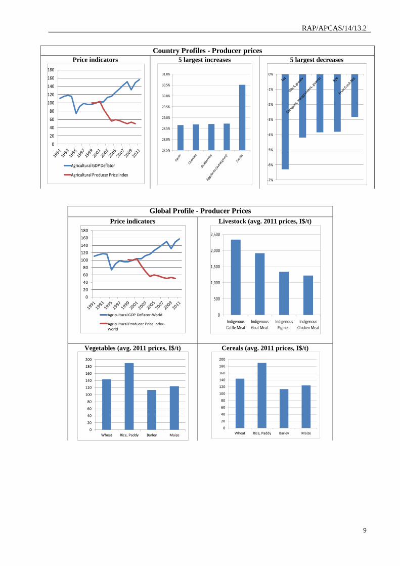
e. Price profiles and other analytical products
FAO has begun quarterly dissemination of regional and global food CPIs accompanied by a
statistical analysis and media release to promote awareness of its new data series. As FAO
progressively expands its price data and indicators, it plans to integrate and present them in
country, regional and global price profiles. Country profiles would show country specific
information on producer prices (absolute levels and indices), consumer prices (indices) and price
transmission coefficients; while regional and global profiles would present regional and global
PPIs and food CPIs, and average price levels for select commodities. Some possible mock-ups
are provided below, for discussion.
RAP/APCAS/14/13.2
9
Country Profiles - Producer prices
Price indicators
5 largest increases
5 largest decreases
Global Profile - Producer Prices
Price indicators
Livestock (avg. 2011 prices, I$/t)
Vegetables (avg. 2011 prices, I$/t)
Cereals (avg. 2011 prices, I$/t)
0
20
40
60
80
100
120
140
160
180
Agricultural GDP Deflator
Agricultural Producer Price Index
27.5%
28.0%
28.5%
29.0%
29.5%
30.0%
30.5%
31.0%
-7%
-6%
-5%
-4%
-3%
-2%
-1%
0%
0
20
40
60
80
100
120
140
160
180
Agricultural GDP Deflator-World
Agricultural Producer Price Index-World
0
500
1,000
1,500
2,000
2,500
Indigenous Cattle Meat
Indigenous Goat Meat
Indigenous Pigmeat
Indigenous Chicken Meat
0
20
40
60
80
100
120
140
160
180
200
Wheat Rice, Paddy Barley Maize
0
20
40
60
80
100
120
140
160
180
200
Wheat Rice, Paddy Barley Maize

RAP/APCAS/14/13.2
10
4. Investment Statistics - Introduction
Raising agricultural productivity is critical to increasing the real incomes necessary for
better access to food7. In turn, increasing capital stock per worker, often known as the capital-
labour ratio, or degree of capital intensity, is a critical to increasing agricultural productivity. In
many instances, the income gap between high-income and low-income countries has widened as a
result of low capital-labour ratios in low-income countries. This reflects both the higher relative
costs of capital compared to labour in low-income countries, but more importantly, weaker credit
markets that make it more difficult for agricultural producers to finance capital investments.
As shown in Figure 2, developing countries exhibit a strong positive correlation between
investment in agriculture, as measured by capital accumulation, and hunger reduction, measured
by the World Food Summit (WFS) goal to eradicate hunger and reduce the number of
undernourished. The graph shows that all countries with the largest setback vis-à-vis the WFS
goal, except DPR Korea, had a negative annual growth rate in Agricultural Capital Stock (ACS)
per worker in agriculture for 1990-2005, while the opposite occurred in countries with the greatest
progress towards the WFS goal.
Figure 2: Annual rates of ACS growth (1990-2005): best and worst performing countries
Source: Von Cramon-Taubadel et al. (2009)
To support analysis of ACS, and its’ associated sources of investment financing, FAO
Statistics Division (ESS) is developing a new and more robust methodology to measure ACS , a
new global Investment Dataset comprised of five main elements - Credit to Agriculture,
Government Expenditures on Agriculture, Official Development Assistance to Agriculture,
7 For a review of the magnitude of, trends in, and data gaps pertaining to investment in agriculture, see ESA Working
Paper No.11-19 Financial Resource Flows to Agriculture (http://www.fao.org/docrep/015/an108e/an108e00.pdf) and
the 2012 State of Food and Agriculture (http://www.fao.org/publications/sofa/en/)

RAP/APCAS/14/13.2
11
Foreign Direct Investment in Agriculture, and Foreign Remittances, and country-level profiles on
both growth in agricultural capital stock and its financing sources. A key feature of this initiative
is the harmonization of FAO work with that of other international organizations that are
compiling relevant datasets, as presented in the following sections. The FAOSTAT’s framework
of agricultural investment flows is illustrated in the following hierarchical chart.
Figure 1. FAOSTAT’s Agricultural Investment Data Framework8
5. Current and planned work on Investment
a. AGRICULTURAL CAPITAL STOCK
FAO’s previous database on ACS was based on FAOSTAT’s physical inventories, which
included the following components: land development, plantation crops, machinery and
equipments, livestock, and structures for livestock. These data excluded the forestry and fishery
subsectors and greenhouse production structures, mainly due to lack of information. The more
significant problem in the ACS database, however, came from limitations in the underlying data
sources, much of which was found in agricultural machinery and equipment data, the
methodology of which is currently being reviewed.
To build a more robust global ACS database, the Statistics Division of FAO (ESS) will
develop a methodology based on national accounts information, and draw on national accounts
data and estimates compiled by the UN Statistics Division and the OECD. To estimate capital
stock data for the agriculture, forestry and fisheries sectors from a national accounts perspective,
it will use country-level data and estimates of the following variables: value-added, gross output,
gross fixed capital formation (GFCF), capital stock, employment and labour compensation. As a
result, the revised methodology would enable FAO to better estimate agricultural capital stock
8 This framework could be further expanded by including other financing sources as Tax Expenditures (Marginal Tax
Revenue Forgone) in Public Domestic or Savings and Firm Product Financing in Private Domestic.
Agricultural Capital Formation (ACF)
ACFt = ACSt – ACSt-1
Domestic Flows
Private Domestic
Credit, Private Equities,
Remittances
Public Domestic
Government Expenditure
Foreign Flows
Private Foreign
Foreign Direct Investment
Foreign Remittances
Public Foreign
ODA + Other Official Flows
RAP/APCAS/14/13.2
12
encompassing agriculture, forestry, and fishing activities more broadly, and thereby enabling
better analysis of productivity and investment financing in the broad agricultural sector.
In addition to improving data on capital stock/physical investment, ESS is also expanding its
coverage of sources of investment financing, looking at both public and private sources, as well as
domestic and foreign sources, as outlined in Figure 1. This is a critical first step in assessing how
the composition of financing sources impacts total investment in agriculture, as well as investment
across different sizes and types of agricultural producers.
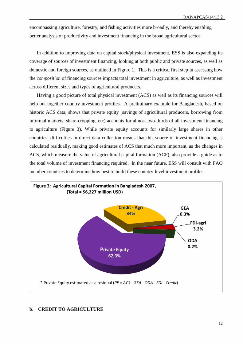
Having a good picture of total physical investment (ACS) as well as its financing sources will
help put together country investment profiles. A preliminary example for Bangladesh, based on
historic ACS data, shows that private equity (savings of agricultural producers, borrowing from
informal markets, share-cropping, etc) accounts for almost two-thirds of all investment financing
to agriculture (Figure 3). While private equity accounts for similarly large shares in other
countries, difficulties in direct data collection means that this source of investment financing is
calculated residually, making good estimates of ACS that much more important, as the changes in
ACS, which measure the value of agricultural capital formation (ACF), also provide a guide as to
the total volume of investment financing required. In the near future, ESS will consult with FAO
member countries to determine how best to build these country-level investment profiles.
b. CREDIT TO AGRICULTURE
GEA 0.3%
FDI-agri 3.2%
ODA 0.2%
Private Equity
62.3%
Credit - Agri 34%
Figure 3: Agricultural Capital Formation in Bangladesh 2007, (Total = $6,227 million USD)
* Private Equity estimated as a residual (PE = ACS - GEA - ODA - FDI - Credit)

RAP/APCAS/14/13.2
13
The extent to which formal private sector credit markets provide investment financing has a
direct and positive correlation with growth in agricultural capital stock, and in turn, with
agricultural productivity growth. This occurs because financial institutions in formal credit
markets are better able to diversify and absorb risks across time, across borrowers, and across
sectors, thereby lowering financing costs to borrowers, and better allocating savings. This source
of financing is of particularly importance in sectors, such as agriculture, where producers face
high risks not only in terms of the timing between the need to finance investments and the
realization of income to repay loans, but also from the significant supply-side uncertainties that
arise from climate and weather conditions (droughts, floods, etc), price volatility of their output,
and the impact of pests and disease, which affect the volume and quality of their output.
Data on formal credit extended to agriculture ― including finance to corporations and firms
for onward financing to farmers, agricultural cooperatives and agri-related businesses ― is
generally available through monetary and financial statistics. This data, which serves as a
benchmark indicator of formal domestic private sector investment activity, is being developed by
FAO’s Statistics Division into a comprehensive credit to agriculture dataset, harvesting official
data from Central Banks websites. Data challenges exist for countries that lack legislative
reporting requirements for this type of data, or where reported data lack the necessary level of
sector detail. Across all countries, a significant challenge also exists in differentiating agricultural
loans for investment purposes, and those for consumption purposes.
c. GOVERNMENT EXPENDITURES ON AGRICULTURE
Although the private sector mobilizes most investment financing in agriculture, the public
sector ― general government units and public (financial and nonfinancial) corporations ― also
plays a role. The efficiency of these expenditures, whether measured in relation to agricultural
GDP, to total government outlays, or the agricultural labour force, remains a key element of the
overall policy mix. Well targeted government expenditures can create a conducive environment
for private investment (economic incentives) and can ensure sufficient availability of public goods
(basic rural infrastructure and market openness), particularly when these investments address
market failures.
The share of government expenditures on agriculture (GEA) is not related in any simple way
to the size of the agricultural sector, and depends inter alia on the overall importance given to
economic functions in governments’ budgets. By bringing together the data on agriculture's shares
in GDP and overall government expenditure we can construct an "agricultural orientation index"
by dividing the agricultural expenditure share of total government expenditures by the agriculture

RAP/APCAS/14/13.2
14
share of GDP, which reflects the relative importance that government places on its agricultural
sector. In Bangladesh, for example, the agriculture share of GDP was significantly higher than
the agricultural share of government expenditures (Figure 4), leading to an agricultural orientation
index up to 5% from 2001 to 1007, rising steadily to 15% in 2011 following the food price crisis.
Despite the need for comprehensive time series data on government expenditures on
agriculture and rural development, such data remain scarce. To address this gap and ensure
comparable data aligned with international standards, ESS, in collaboration with the IMF
Statistics Department, developed a Government Expenditures on Agriculture questionnaire based
on the Government Finance Statistics Manual, 2001 (GFSM 2001) methodology. ESS launched
this questionnaire globally in 2012, requesting additional detail on the agriculture subsectors of
agriculture, forestry and fisheries, as well as data on environmental protection. The questionnaire
also looks for additional detail on recurrent and capital expenditures, in order to proxy the amount
of expenditures allocated for investment. The second annual global data collection is currently
underway.
.
d. OFFICIAL DEVELOPMENT ASSISTANCE TO AGRICULTURE
Official Development Assistance to Agriculture (ODA) from major bilateral and multilateral
donors is an important complement to domestic sources of agricultural financing. To obtain this
data, ESS harvests data from the OECD’s Creditor Reporting System (CRS), which records ODA
-0.10
0.00
0.10
0.20
0.30
0.40
0.50
0.60
0%
5%
10%
15%
20%
25%
30%
35%
2001 2002 2003 2004 2005 2006 2007 2008 2009 2010 2011
Figure 4: Government Expenditure on Agriculture - Bangladesh
GEA as % of Total Government Outlays (Left Axis)
Agriculture Value Added as % of GDP (Left Axis)
Agricultural Orientation Index (Right Axis)

RAP/APCAS/14/13.2
15
and Other Official Flows (OOF) at the project level. By extracting the subset of the data relevant
for agriculture, rural development and food security, ESS is able to obtain necessary data without
creating duplication across international organizations, or imposing additional response burden on
countries. Where data gaps exist, ESS will work with the OECD to identify and address these
gaps. The first comprehensive ODA to agriculture data will be available in FAOSTAT in the near
future.
e. FOREIGN DIRECT INVESTMENT
A fourth source of agricultural investment financing comes from foreign direct investment
(FDI). A host of factors, including spikes in food and fuel prices, a desire by countries dependent
on food imports to secure food supplies in the face of uncertainty, and speculation on land and
commodity price increases, recently prompted a sharp increase in investment involving significant
use of agricultural land, water, and forested areas in developing and transition countries. In the
coming year, ESS will work with data from UNCTAD to develop a database on FDI to
agriculture, and examine data gaps and challenges, along with strategies to address them.
f. FOREIGN REMITTANCES
A fifth source of investment financing comes from foreign remittances, or the money sent to
home countries by migrants. Last October the World Bank estimated that developing countries
would receive $414 billion US in foreign remittances in 2013, an increase of 6.3% over the
previous year. To put this in perspective, foreign remittances to Tajikstan would account for half
of its GDP, and for three times the FDI to India, which received $71 billion in remittances. As
such, foreign remittances are important due to their size, but also because they act as an automatic
economic stabilizer, rising in value when domestic currency weakens. A challenge that faces ESS
in including this source of investment financing is the determination of the share goes towards
financing agriculture, and the subset that finances agricultural investment.
6. INVITATIONS TO APCAS MEMBER COUNTRIES
APCAS member countries are requested to provide comments and feedback on these existing and
new lines of work, and suggestions on improvements and opportunities for collaboration in the
domains of price and investment statistics.
Questions, inputs and advice can be e-mailed to Ms. Dubey ([email protected]),
Franck Cachia ([email protected]) or Fabiana Cerasa ([email protected])