ashrae research project report 1635-rp library/technical resources/covid-19/ashra… · figure 2-5....

ASHRAE Research Project Report 1635-RP

SIMPLIFIED PROCEDURE FOR CALCULATING EXHAUST/INTAKE SEPARATION DISTANCES

Approval: January 2016

Contractor: CPP, Inc. 2400 Midpoint Drive, Suite 190 Fort Collins, CO 80525 Principal Investigator: Ronald L. Petersen Authors: Jared Ritter, Anthony Bova, John Carter

Author Affiliations, Wind Engineering and Air Quality Consultants, CPP, Inc.

Sponsoring Committee: TC - Ventilation Requirements & Infiltration

Co-Sponsoring Committee: N/A Co-Sponsoring Organizations: N/A

Shaping Tomorrow’s Built Environment Today

©2012 ASHRAE www.ashrae.org. This material may not be copied nor distributed in either paper or digital form without ASHRAE’s permission. Requests for this report should be directed to the ASHRAE Manager of Research and Technical Services.

http://www.ashrae.org/

FINAL REPORT

SIMPLIFIED PROCEDURE FOR CALCULATING

EXHAUST/INTAKE SEPARATION DISTANCES

AMERICAN SOCIETY OF HEATING, REFRIGERATING, AND AIR-

CONDITIONING ENGINEERS, INC.

RESEARCH PROJECT 1635-TRP CPP Project 7499

Prepared for:

The American Society of Heating, Refrigerating,

and Air-Conditioning Engineers, Inc.

1791 Tullie Circle

Atlanta, Georgia 30329

Prepared by:

Ronald L. Petersen, PhD, CCM, FASHRAE

Jared Ritter

Anthony Bova

John C. Carter, MS, MASHRAE

23 September 2015

iii

EXECUTIVE SUMMARY

This research was sponsored by ASHRAE Technical Committee (TC) 4.3. The purpose of

this Research Project is to provide a simple, yet accurate procedure for calculating the minimum

distance required between the outlet of an exhaust system and the outdoor air intake to a

ventilation system to avoid re-entrainment of exhaust gases. The new procedure addresses the

technical deficiencies in the simplified equations and tables that are currently in Standard 62.1-

2013 Ventilation for Acceptable Indoor Air Quality and model building codes. This new

procedure makes use of the knowledge provided in Chapter 45 of the 2015 ASHRAE

Handbook—Applications, and was tested against various physical modeling and full-scale

studies.

The study demonstrated that the new method is more accurate than the existing Standard 62.1

equation which under-predicts and over-predicts observed dilution more frequently than the new

method. In addition, the new method accounts for the following additional important variables:

stack height, wind speed and hidden versus visible intakes. The new method also has theoretically

justified procedures for addressing heated exhaust, louvered exhaust, capped heated exhaust and

horizontal exhaust that is pointed away from the intake.

Included in the report are recommendations and documentation regarding minimum dilution

factors for Class 1-4, wood burning kitchen, boiler, vehicle, emergency generator and cooling

tower type exhaust.

v

TABLE OF CONTENTS

EXECUTIVE SUMMARY ............................................................................................................ iii

TABLE OF CONTENTS ................................................................................................................. v

LIST OF FIGURES ....................................................................................................................... vii

LIST OF TABLES .......................................................................................................................... ix

1. INTRODUCTION ..................................................................................................................... 1

2. REVIEW AND EVALUATION OF STANDARD 62.1 EQUATION ..................................... 4 2.1 General ................................................................................................................................ 4 2.2 Background on Standard 62.1-2013 Equation ..................................................................... 4 2.3 Evaluation of Existing Standard 62.1 Equation .................................................................. 5 2.4 Dilution Databases .............................................................................................................. 8

2.4.1 Database 1 – Wilson and Chui, 1994 ......................................................................... 8 2.4.2 Database 2 – Wilson and Lamb, 1994 ...................................................................... 11 2.4.3 Database 3 – ASHRAE Research Project 805, Petersen, et.al, 1997 ....................... 12 2.4.4 Database 4 – Hajra and Stathopoulos, 2012 ............................................................. 16 2.4.5 Database 5 – Schulman and Scire, 1991 .................................................................. 18

2.5 Dilution Equation Performance Metrics ............................................................................ 20 2.6 Evaluation of Standard 62.1 Equation Against Databases 1 and 2 ................................... 21

3. DEVELOPMENT AND EVALUATION OF NEW STANDARD 62.1 EQUATION ........... 25 3.1 New Equation Development.............................................................................................. 25

3.1.1 New Equation 1 Development (New1) .................................................................... 25 3.1.2 New Equation 2 Development (New2) .................................................................... 28 3.1.3 New Equation 3 Development .................................................................................. 29 3.1.4 New Equation 4 Development .................................................................................. 31

4. EVALUATION OF 62.1 EQUATION AND NEW EQUATIONS ........................................ 33 4.1 ASHRAE Research Project (RP) 805 – 0 Degree Wind Direction (Petersen, et al.,

1997) .................................................................................................................................. 33 4.2 ASHRAE Research Project 805 , 45 Degree Wind Direction (Petersen, et al., 1997) ...... 34 4.3 Hajra and Stathopoulos (2012) .......................................................................................... 36 4.4 Schulman and Scire (1991) ............................................................................................... 38 4.5 Sidewall (Hidden) Intakes ................................................................................................. 40

5. DEVELOPMENT OF REFINED DILUTION FACTORS ..................................................... 42 5.1 Background and Objective ................................................................................................ 42 5.2 General Factors to Consider ............................................................................................. 44 5.3 Recommended Dilution Factors ........................................................................................ 46

5.3.1 Combustion Type Sources ........................................................................................ 46 5.3.1.1 General ....................................................................................................... 46 5.3.1.2 Diesel generators and diesel vehicles ......................................................... 48 5.3.1.3 Light duty gas vehicles .............................................................................. 48 5.3.1.4 Boilers ........................................................................................................ 50

5.3.2 Kitchen ..................................................................................................................... 51

vi

5.3.3 Cooling Tower .......................................................................................................... 52 5.3.4 Toilet ........................................................................................................................ 52

5.4 Summary of Recommended Values and Discussion ......................................................... 54

6. UPDATED SEPARATION DISTANCE METHODOLOGY ................................................ 56 6.1 Calculated Separation Distances (General and Regulatory Procedure) ............................ 56 6.2 General Equation and Method ........................................................................................... 56 6.3 Special Cases ..................................................................................................................... 61

6.3.1 Horizontal Exhaust ................................................................................................... 61 6.3.2 Upblast and Downblast Exhaust ............................................................................... 61 6.3.3 Hidden Intakes .......................................................................................................... 62 6.3.4 Heated Exhaust ......................................................................................................... 63 6.3.5 Capped Heated Exhaust ............................................................................................ 64

6.4 Example Calculations ........................................................................................................ 66 6.4.1 Class 1 Exhaust ........................................................................................................ 66 6.4.2 Class 2 Exhaust ........................................................................................................ 67 6.4.3 Class 3 Exhaust ........................................................................................................ 68 6.4.4 Class 4 Exhaust ........................................................................................................ 69 6.4.5 Boiler Exhaust (Capped and Heated) ....................................................................... 70

7. CONCLUSIONS ..................................................................................................................... 71

8. REFERENCES ........................................................................................................................ 73

vii

LIST OF FIGURES

Figure 2-1. Building models with intake sampling areas shown shaded from Wilson and Chiu

(1994). ...................................................................................................................................... 10

Figure 2-2. Typical predicted versus observed dilution results from Wilson and Chiu (1994). ... 10

Figure 2-3. Full-scale building configuration from Wilson and Lamb (1994). .............................. 11

Figure 2-4. Predicted and observed dilution versus normalized distance from Wilson and

Lamb (1994). ........................................................................................................................... 12

Figure 2-5. Test building and rooftop receptor layout used for the ASHRAE RP 805

Evaluation, Petersen, et.al. (1997). .......................................................................................... 14

Figure 2-6. Drawing showing observed dilution versus string distance from ASHRAE RP

805 – 0 degree data, Petersen, et.al (1997). ............................................................................. 15

Figure 2-7. Drawing showing observed dilution versus string distance from ASHRAE RP

805 – 45 degree data, Petersen, et.al (1997). ........................................................................... 16

Figure 2-8. Drawing showing building, exhaust and receptor configuration from Hajra and

Stathopoulos (2012). ................................................................................................................ 17

Figure 2-9. Drawing showing observed dilution versus string distance from Hajra and

Stathopoulos (2012). ................................................................................................................ 18

Figure 2-10. Test building and rooftop receptor layout used for the Schulman and Scire

Database (1991). ...................................................................................................................... 19

Figure 2-11. Drawing showing observed dilution versus string distance from Schulman and

Scire (1991). ............................................................................................................................. 20

Figure 2-12. Predicted minimum dilution versus dimensionless sting distance using Standard

62.1 equation and other more accurate equations. ................................................................... 22

Figure 3-1. Comparison of New Equation 1 predictions versus Wilson and Chui and Wilson

and Lamb. ................................................................................................................................ 28

Figure 3-2. Comparison of New Equation 2 predictions versus Wilson and Chui and Wilson

and Lamb. ................................................................................................................................ 29

Figure 3-3. Comparison of New3 predictions versus Wilson and Chui and Wilson and Lamb. .... 30

Figure 3-4. Comparison of New1, New2 and New3 predictions versus Wilson and Lamb. .......... 31

Figure 3-5. Comparison of New4 with New1, New2 and New3 .................................................. 32

Figure 4-1. Comparison of New1, New2 and New4 predictions versus ASHRAE RP 805 - 0

degree wind direction. .............................................................................................................. 34


degree wind direction. .............................................................................................................. 35

Figure 4-3. Ratio of predicted (ASHRAE 62.1) to observed dilution versus string distance

using Hajra and Stathopoulos (2012) database – all data, i=0.1527. ....................................... 37

Figure 4-4. Ratio of predicted (ASHRAE 62.1) to observed dilution versus string distance

using Hajra and Stathopoulos (2012) database – all data, i=0.175. ......................................... 38

CPP, Inc. viii Project 7499

viii

Figure 4-5. Ratio of predicted (Standard 62.1) to observed dilution versus string distance

using Schulman and Scire (1991) database. ............................................................................. 39

Figure 4-6. Comparison of New1, New2 and New4 predictions versus ASHRAE RP 805 and

Schulman - hidden intake data. ................................................................................................ 41

Figure 6-1. Diagram showing how to calculate string distance, L. In the figure L = L1+L2+L3 .. 59

Figure 6-2 Typical Upblast Exhaust ............................................................................................... 61

ix

LIST OF TABLES

Table 2-1. Tables F-1 and F-2 From Standard 62.1-2013. ............................................................... 4

Table 2-2. Example Calculations Using Standard 62.1-2013 Method. ............................................ 5

Table 2-3. Building and exhaust flow configurations from Wilson and Chiu, 1994 ........................ 9

Table 4-1. Comparison of New Equation predictions versus ASHRAE RP 805 – 0 degree

data. .......................................................................................................................................... 33

Table 4-2. Comparison of New Equation predictions versus ASHRAE RP 805 – 45 degree

data. .......................................................................................................................................... 35

Table 4-3. Comparison of Standard 62.1 and New3 predictions versus Hajra data – i=0.1527 ..... 36

Table 4-4. Comparison of Standard 62.1 and New3 predictions versus Hajra data – i=0.175 ....... 37

Table 4-5. Comparison of Standard 62.1 and New4 predictions versus Schulman data ................ 39

Table 4-6. Comparison of New Equation predictions versus ASHRAE Research Project 805 –

Hidden Intake Data .................................................................................................................. 41

Table 5-1 Minimum Separation Distances and Dilution Factors From Standard 62.1 ................. 44

Table 5-2. Summary of Minimum Separation Distances and Dilution Criteria From Standard

62-1989R. As indicated, an equation was used to calculate the minimum separation

distance based on the Minimum Dilution Factor. Distances were not specified. ................... 44

Table 5-3. Health and Odor Thresholds for Combustion Equipment ............................................. 47

Table 5-4. Minimum dilution factor calculation for light duty gasoline vehicles .......................... 49

Table 5-5. Calculation of Dilution Targets for Boiler Exhaust. ..................................................... 50

Table 5-6. Odor detection thresholds reported for methanethiol. ................................................... 53

Table 5-7. Summary of Toilet Exhaust Odor Study Results .......................................................... 54

Table 5-8. Summary of Recommended Minimum Dilution Factors, DF ....................................... 55

Table 6-1 Example Spreadsheet for Use in Calculating Separation Distances ............................. 60

Table 6-2. Class 1 Exhaust Example Calculation ........................................................................... 66



Table 6-5. Class 4 Exhaust Example Calculation .......................................................................... 69

Table 6-6. Boiler Exhaust Example Calculation ............................................................................ 70

1

1. INTRODUCTION

Currently ASHRAE Standard 62.1-2013 (Standard 62.1) has air intake minimum separations

distances, L, specified for various types of exhaust sources in Table 5-1 of the Standard. The

minimum separation distance is defined as the shortest “stretched string” distance from the

closest point of the outlet opening to the closest point of the outdoor air intake opening or

operable window, skylight, or door opening, along a trajectory as if a string were stretched

between them. Other codes and standards (e.g., 2012 Uniform Mechanical Code, U.S., Building

Codes, Uniform Plumbing Code) also specify minimum separation distances, all of which appear

to be “rule of thumb” based with 3 to 10 ft (1 to3 m) being the magic number for most exhaust

types. The separation distances can be both far too lenient and far too restrictive, depending on

the type of exhaust and exhaust and intake configurations.

Both code and Standard 62.1 requirements are overly simplistic and fail to account for

significant variables such as the exhaust airflow rate, the enhanced mixing caused by high

exhaust discharge velocity, the orientation of the discharge, or the height of the exhaust relative to

intake. Standard 62.1 also includes an informative Appendix F that outlines a procedure to

account for exhaust air flow rate and velocity to achieve target dilution levels. The appendix is

not mandatory but given as an example of how to use analytical techniques to show that

separation distances other than those in Table 5-1 are acceptable.

The purpose of this Research Project is to provide a simple, yet accurate procedure for

calculating the minimum distance required between the outlet of an exhaust system and the

outdoor air intake to a ventilation system to avoid re-entrainment of exhaust gases. The procedure

addresses the technical deficiencies in the simplified equations and tables that are currently in

Standard 62.1. This new procedure makes use of the knowledge provided in Chapter 45 of the

2015 ASHRAE Handbook—Applications, and various wind tunnel and full-scale studies

discussed herein.

The updated methodology is suitable for standard HVAC engineering practice and has as

independent variables: exhaust outlet velocity; exhaust air volumetric flow rate; exhaust outlet

configuration (capped/uncapped) and position relative to intake orientation and position; desired

dilution ratio; and ambient wind speed. The current Appendix F method includes some of these

factors but does not include variable wind speed, stack height, or hidden intake reduction factors.

The method discussed herein takes into account all of these variables.

CPP, Inc. 2 Project 7499

The research started out with an objective to develop two new procedures from existing and

new research with the following characteristics:

• Procedure 1.

o A general procedure suitable for standard HVAC engineering practice that has as

independent variables: exhaust outlet velocity; exhaust air volumetric flow rate;

exhaust outlet configuration (capped/uncapped/horizontal/louvered) and position

(vertical separation distance); exhaust direction; desired dilution ratio; hidden

intakes (building sidewall), and ambient wind speed.

o Other factors, such as location relative to walls and edge of building, geometry of

the exhaust discharge and inlets, etc., are reduced to fixed assumptions that are

reasonable yet somewhat conservative.

• Procedure 2.

o A regulatory procedure suitable for Standard 62.1, Standard 62.2, and model

building codes that has as independent variables only exhaust outlet velocity,

exhaust air volumetric flow rate, desired dilution ratio, and a simple way to

account for orientation relative to the inlet.

o All other variables will be reduced to fixed assumptions that are reasonable yet

conservative.

o This procedure consists of tabulated distances for various classes of exhaust.

In the end, one simple procedure was developed that met the overall objectives of the study

and is appropriate for the following exhaust types.

• Toilet exhaust from rain-capped vents or dome exhaust fans

• Grease and other kitchen fan exhausts

• Combustion flues and vents with either forced or natural draft discharge in horizontal or

vertical direction, with and without flue caps (this includes diesel generators)

• Diesel vehicle emissions

• Building exhaust at indoor air temperature through louvered or hooded vents

• Plumbing vents

• Cooling towers

The method does not address:

• Laboratory and industrial ventilation process exhausts


• Large, industrial sized combustion flues and stacks

• Packaged units that have integral exhaust and intake locations

A secondary objective of this project is to address dilution targets, a necessary parameter for

calculating the separation distance calculation. Accordingly, minimum dilution factors were

reviewed and updated for various types of exhausts as appropriate, especially those with known

emissions and health impacts such as combustion exhaust.

The following sections provide a review of the Standard 62.1 equation, discussion of data

bases that were used to test and compare the Standard 62.1 equation and new equations,

development of a new equation, an evaluation of the new and Standard 62.1 equations against

observations, development of minimum dilution values, and a section discussing the updated new

methodology.

4

2. REVIEW AND EVALUATION OF STANDARD 62.1 EQUATION

2.1 GENERAL

This section provides background information on the existing Standard 62.1-2013 equation

(hereafter referred to as 62.1 equation), a description of dilution databases that will be used to

evaluate the 62.1 equation and future equation, and an evaluation of the 62.1 equation against the

database.

2.2 BACKGROUND ON STANDARD 62.1-2013 EQUATION

The following discussion illustrates some of the problems with the current Standard 62.1

methodology. Appendix F of Standard 62.1 provides the following tables for Class 3 and Class 4

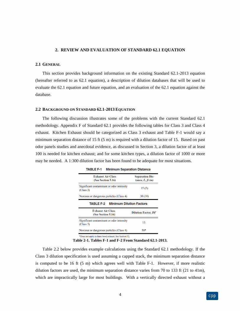
exhaust. Kitchen Exhaust should be categorized as Class 3 exhaust and Table F-1 would say a

minimum separation distance of 15 ft (5 m) is required with a dilution factor of 15. Based on past

odor panels studies and anecdotal evidence, as discussed in Section 3, a dilution factor of at least

100 is needed for kitchen exhaust; and for some kitchen types, a dilution factor of 1000 or more

may be needed. A 1:300 dilution factor has been found to be adequate for most situations.

Table 2-1. Tables F-1 and F-2 From Standard 62.1-2013.

Table 2.2 below provides example calculations using the Standard 62.1 methodology. If the

Class 3 dilution specification is used assuming a capped stack, the minimum separation distance

is computed to be 16 ft (5 m) which agrees well with Table F-1. However, if more realistic

dilution factors are used, the minimum separation distance varies from 70 to 133 ft (21 to 41m),

which are impractically large for most buildings. With a vertically directed exhaust without a


cap, the separation distances decrease and vary from 6 to 123 ft (2 to 38 m). These results point

out several problems with the current method for kitchen exhaust:

Table 2-2. Example Calculations Using Standard 62.1-2013 Method.

the specified minimum separation distance in Table F-1 will not ensure the intake is

protected from odors for most kitchen exhaust (e.g., capped or low exit velocity);

If a vertically directed exhaust is used with a short stack, the Appendix F method will

allow the intake to be very close to the exhaust, a poor design from an odor perspective

since a higher wind condition may result in no plume rise and direct plume impact on the

intake;

The method does not account for stack height. For a tall stack and vertically directed

exhaust, the best intake location will be close to the stack versus farther away directly in

conflict with the Table 1 results.

The method does not account for the added dilution, except in the form of the string

distance, if the intake and exhaust are blocked by a screen wall.

The method does not allow for increased dilution if the intake is on a building sidewall

due to the increased turbulence.

2.3 EVALUATION OF EXISTING STANDARD 62.1 EQUATION

The development of the 62.1 equation can be found in Appendix N of the August 1996 Public

Review Draft of the ASHRAE Standard 62, which will be referred to as 62-1989R. The equation

development begins with the minimum dilution equation (Dmin) found in the 1993 ASHRAE

Handbook, Fundamentals, Chapter 14 and Wilson and Lamb (1994).

𝐷𝑚𝑖𝑛 = [𝐷𝑜0.5 + 𝐷𝑠

0.5]2 (2.1)

Table 1. Example Minimum Separation Distance Results Based on Appendix F

Case Dilution

Factor

Exhaust Flow

cfm

Dischange

Velocity

fpm

Separation

Distance

ft

Capped Stack

Appendix F 15 2000 0 16

CPP's recommended value 300 2000 0 70

Grill/Range Hood

- Odor Panel Results 570 2000 0 96

Rotisserie Exhaust


Heated Vertically Directed with no Cap, Unheated

Appendix F 15 2000 1000 6

CPP's recommended value 300 2000 1000 60

Grill/Range Hood


Rotisserie Exhaust



where:

𝐷𝑜 = 1 + 𝐶1𝛽 (𝑉𝑒

𝑈𝐻 )

2 (2.2)

𝐷𝑠 = 𝛽1 (𝑆2𝑈𝐻

𝑄𝑒 ) (2.3)

Do represents the initial jet dilution and Ds represents the dilution that occurs versus

separation distance. 62-1989R states that the constant C1 ranges from 1.6 to 7, β1 (C2 in 62-

1989R) ranges from 0.0625 to 0.25, S is the “stretched string” distance measured along a

trajectory, UH is the wind speed at the roof level, Ve is the discharge velocity, Qe is the volume

flow rate, and β is a factor that relates the nature of discharge outlet. β equals 1 for the vertical

discharge and 0 for a capped (or downward) discharge.

To develop the Standard 62.1 equation, equations 2.1, 2.2 and 2.3 were first rearranged to

solve for S (L in the Standard 62.1 Equation) which results in.

𝑆 = [𝑄𝑒

𝛽1𝑈𝐻]

0.5[𝐷0.5 − (1 + 𝐶1𝛽 (

𝑉𝑒

𝑈𝐻)

2)

0.5

] (2.4)

The equation is then simplified by assuming (62-1989R):

the 1 term insignificant,

Ve = 0 for capped or non-vertical stacks,

UH = 2.5 m/s (500 fpm) average wind speed,

C1 = 1.7 (on the low end of the range, giving less credit for dilution due to discharge

velocity which tends to increase the separation distance), and

β1 = 0.25 (on the high end of the range, giving maximum credit for dilution due to

separation, and tends to reduce separation distance, and is non-conservative),

The Standard 62.1 equation then results, or

𝑆 = 0.09 𝑄𝑒0.5 [𝐷0.5 −

𝑉𝑒

400 ] (in feet) (2.5)

𝑆 = 0.04 𝑄𝑒0.5 [𝐷0.5 −

𝑉𝑒

2 ] (in meters) (2.6)

where


Qe = exhaust air volume, cfm (L/s).

D = dilution factor for the exhaust type of concern.

Ve = exhaust air discharge velocity, fpm (m/s).

Ve is positive when the exhaust is directed away from the outside air intake at a

direction that is greater than 45° from the direction of a line drawn from the closest

exhaust point the edge of the intake;

Ve has a negative value when the exhaust is directed toward the intake bounded by

lines drawn from the closest exhaust point the edge of the intake; and

Ve is set to zero for other exhaust air directions regardless of actual velocity. Ve is

also set to 0 for vents from gravity (atmospheric) fuel-fired appliances, plumbing

vents, and other non-powered exhausts, or if the exhaust discharge is covered by a

cap or other device that dissipates the exhaust airstream.

For hot gas exhausts such as combustion products, an effective additional 500 fpm

(2.5 m/s) upward velocity is added to the actual discharge velocity if the exhaust

stream is aimed directly upward and unimpeded by devices such as flue caps or

louvers.

Equation 2.6 has the following problems in addition to those discussed in Section 2.1:

The equation in only valid for a flush vents and does not account for stack height or

height difference between the stack and air intake.

Even though an exit velocity term is included, it does not adequately account for high

velocity exhaust systems. The velocity term is accounts for the added dilution due to

a higher exit velocity but does not account for the added plume rise.

The assumed value for the constants C1 or 1.7, while conservative, is not supported

by the research. According to Wilson and Chiu (1994) and ASHRAE (1993, 1997),

values of 7 and 13 are more appropriate.

The assumed value for the constant β1 of 0.25 is non- conservative and is not

supported by the research. According to Wilson and Chiu and ASHRAE

(1993,1997), values ranging from 0.04 to 0.08 are more appropriate.

For vertical stacks, a wind speed higher than 2.5 m/s (500 fpm) may be critical

because plume rise will decrease as wind speed increases, while at low wind speed

the plume rise will be very large.


For flush vents and capped stacks, a wind speed lower than 2.5 m/s (500 fpm) will

most likely be the critical case. Speeds as low as 1 m/s (200 fpm) can occur a

significant fraction of the time.

Setting Ve equal to a negative number when the exhaust is directed away from the

intake, while intuitively correct, cannot be derived from the original equation used to

develop the Standard 62.1 approach.

To evaluate the Standard 62.1 equation, the equation will be rearranged so dilution can be

predicted for comparison with the dilution values recorded in the databases discussed in Section

2.4. The re-arranged equation is provided below.

𝐷 = (11.1 𝑆

𝑄𝑒0.5 +

𝑉𝑒

400 )

2 (IP)

(2.7)

𝐷 = (25 𝑆

𝑄𝑒0.5 +

𝑉𝑒

2 )

2 (SI)

Overall, this section has shown some of the problems with the current Standard 62.1 equation

and confirms the need for an improved equation.

2.4 DILUTION DATABASES

During this task, existing wind tunnel and full-scale data were assembled and reviewed. Only

those wind tunnel databases that meet the criteria outlined in EPA’s Guideline for Fluid Modeling

of Atmospheric Diffusion (Snyder, 1981) were be used in this study. Some of the important

criteria that were considered are as follows:

A boundary-layer wind profile representative of the atmosphere was established.

The approach turbulence profile was representative of the atmosphere.

Reynolds number independent flow was established

Once the relevant databases were selected, the data were entered into an excel spreadsheet in

a form that will expedite comparisons with Appendix F equations and the other numerical

methods that are developed in Section 3. The following sub-sections discuss each database.

2.4.1 Database 1 – Wilson and Chui, 1994

The following summarizes the important aspects of this database.


1:500 and 1:2000 scale model tests were conducted.

Building Reynolds numbers exceeded 104 to meet Reynolds number independence

criterion of Snyder (1981).

A wind power law exponent of 0.25 was established and wind speeds at building height

of 5.9 to 12.1 m/s (1200 to 2400 fpm) were set.

Eleven model building configurations were tested at six different exhaust momentum

velocity ratios as shown in Table 2-3 and Figure 2-1 below.

Exhaust parameters: flush circular vent with exhaust density ratio varying from 0.14 to

0.38. Momentum ratios varied from 0.8 to 1.5.

Building height to width ratios varied from 1 to 12.

Wilson and Chiu (1994) showed that Equations 2.1, 2.2 and 2.3 above with β1 = 0.625 and C1

= 7 provided a lower bound to the observed dilution values for several building configurations.

This database will not be used directly to evaluate the performance of the new equation rather the

predicted lower bound using Equations 2.1, 2.2 and 2.3 with recommended constants will be used

as a lower bound prediction for comparison purposes.

Table 2-3. Building and exhaust flow configurations from Wilson and Chiu, 1994

Figure 2-2 shows a typical comparison of predicted (Equations 2.1, 2.2 and 2.3) and observed

dilution versus normalized distance. As can be seen the predicted values using equations 2.1, 2.2

and 2.3) provide a lower bound estimate of the observed dilution.


Figure 2-1. Building models with intake sampling areas shown shaded from Wilson and Chiu

(1994).

Figure 2-2. Typical predicted versus observed dilution results from Wilson and Chiu (1994).


2.4.2 Database 2 – Wilson and Lamb, 1994

This is a very unique database in that it is based on a full-scale study that was conducted

using tracer gas released from stacks and exhaust vents on Washington State University

chemistry laboratory buildings “Fulmer” and “Annex”, shown in Figure 2-3. While the database

is based on laboratory exhaust stacks, the results are valid for any type exhaust.

Figure 2-3. Full-scale building configuration from Wilson and Lamb (1994).

The following summarizes the important aspects of this database.

Each test took place on a different day between January 14 and March 11, 1994.

Hourly meteorological data (wind speed, wind direction, temperature and σθ) were

collected from an 8 m (26.25 ft) mast erected on the penthouse roof on the Annex

Building. This represents the tallest point of the test buildings, which minimizes building

wake effects. Wind speeds during the testing period varied from 2.2 to 8.1 m/s (440 to

1600 fpm). Crosswind turbulence indicated by σθ ranged from 6.5 to 24.8 degrees.

Tracer gas dilution measurements were carried out by releasing sulfur hexafluoride (SF6)

from the uncapped fume hood exhaust vents and collecting four sequential hourly

average air samples from 44 locations. The distances ranged from S=5 m (16.4 ft) to S=

270 m (886 ft). Sufficient data was collected to ensure that the minimum dilution could

be documented.

Stack heights ranged from 0 to 3.66 m (0 to 12 ft) and average velocity ratios, M, ranged

from 0.83 to 8.3.


Figure 2-4 below shows the overall results from the study. The figure shows that equations

2.1, 2.2 and 2.3 with β1= 0.04 and C1 = 13 provide a lower bound estimate of dilution when

compared to observations. Again, this confirms the validity of these equations for flush vents

with low plume rise. As with Wilson and Chui (1994), this database will not be used directly to

evaluate the performance of the new equation; rather the predicted lower bound using equations

2.1., 2.2. and 2.3 with the recommended constants from this study will be used as a 2nd

lower

bound prediction for comparison purposes.

Figure 2-4. Predicted and observed dilution versus normalized distance from Wilson and

Lamb (1994).

2.4.3 Database 3 – ASHRAE Research Project 805, Petersen, et.al, 1997

This study was initially commissioned in 1997 as an ASHRAE research project to determine

the influence of architectural screens on exhaust dilution. Wind tunnel experiments were

performed with generic building geometry in order to generate a database of concentrations to

document the effects of several screen wall configurations. Baseline exhaust concentrations

obtained without the presence of a screen wall were also included in the wind tunnel assessment.


The following summarizes the important aspects of this database:

1:50 scale model tests were conducted in the Cermak Peterka Petersen boundary layer

wind tunnel with velocity profile power law exponent of 0.28.

Building Reynolds Number >11,000 to meet Reynolds Number independence criterion of

Snyder (1981).

Concentration data for various different exhaust configurations:

o Building measurements 50’ x 100’ x 50’ (15.2m x 30.48m x 15.2m) (H x W x L)

o Stack heights (hs): 0, 1, 3, 5, 7, 12 ft (0, 0.3, 0.9, 1.5, 2.1, 3.7 m)

o Volumetric flow rate of 500 cfm (0.24 m3/s), 5000 cfm (2.4 m

3/s), 20,000 cfm

(9.43 m3/s)

o Exhaust momentum ratios (M=Ve/UH): ranging from ~1 to 4

o Receptors were placed on rooftop and leeward walls.

o Wind azimuths: 0, 45 and 90 degrees

o Reference wind speed of Uref = 3.7 m/s (728 fpm) and 11.1 m/s (2185 fpm) in the

wind tunnel

For this study, data were only used for results obtained in the wind tunnel for cases with no

screen wall on the test building. Only data collected at receptor locations on the test building were

used, and no downwind or off-building exhaust concentrations were considered. Data for multiple

stack heights, multiple momentum ratios, and wind azimuths of 0 and 45 degrees were considered

in this evaluation. The testing configuration is illustrated in Figure 2-5.


Figure 2-5. Test building and rooftop receptor layout used for the ASHRAE RP 805 Evaluation,

Petersen, et.al. (1997).

Concentration measurement data from the original wind tunnel study were entered in

tablature format into a spreadsheet. Plots of the measured dilution values versus string distance

are provided in Figure 2-6 and Figure 2-7.


Figure 2-6. Drawing showing observed dilution versus string distance from ASHRAE RP 805 –

0 degree data, Petersen, et.al (1997).

Figure 2-6 above shows that the observed dilution increases as stack height is increased.

Similar trends are observed for stacks with similar momentum ratios (e.g. M=1.2 and M=1.9).

For the 0 degree orientation, the furthest rooftop receptor location was located approximately

15 m (49 ft) from the stack. Data taken at distances greater than 15 m (49 ft) indicates

concentrations obtained at a receptor in a “sidewall” location. As expected, a noticeable increase

in dilution is observed at sidewall receptor locations.

1

10

100

1000

10000

100000

1000000

0.00 2.00 4.00 6.00 8.00 10.00 12.00 14.00 16.00 18.00 20.00

Dilu

tio

n

String Distance, S [m]

ASHRAE RP 805 - Dilution Data - (All Data) - 0 degrees 500 cfm, hs=0 ft, M=0.9

500 cfm, has=1 ft, M=0.9

500 cfm, hs=3 ft, M=0.9

500 cfm, hs=7 ft, M=0.9

500 cfm, hs=12 ft, M=0.9

5000 cfm, hs=1 ft, M=3.5

5000 cfm- hs=3 ft, M=3.5

5000 cfm- hs=7 ft, M=3.5

5000 cfm- hs=12 ft, M=3.5

500 cfm, has=0 ft, M=0.3

500 cfm, has=1 ft, M=0.3

500 cfm, has=3 ft, M=0.3

500 cfm, has=7 ft, M=0.3

500 cfm, has=12 ft, M=0.3

5000 cfm, hs=0 ft, M=1.2

5000 cfm, hs= 1 ft, M=1.2

5000 cfm, hs=3 ft, M=1.2

5000 cfm, hs=7 ft, M=1.2

5000 cfm, hs=12 ft, M=1.2

20000 cfm, hs=0 ft, M=1.9

20000 cfm, hs=1 ft, M=1.9

20000 cfm, hs=3 ft, M=1.9

20000 cfm, hs=7 ft, M=1.9

20000 cfm, hs=12 ft, M=1.9


Figure 2-7. Drawing showing observed dilution versus string distance from ASHRAE RP 805 –

45 degree data, Petersen, et.al (1997).

Similar to the 0 degree data, Figure 2-7 shows the most significant increases in dilution occur

with increases vertical stack height. Increases in dilution are also observed for cases with higher

momentum ratios (i.e., M>3). For the 45 degree data set, the furthest rooftop receptor location is

located approximately 13 m (42.7 ft) from the stack. Receptors at a distance greater than 13 m

(42.7 ft) were located on the leeward wall of the building (sidewall receptors). As expected,

dilution values were observed to increase at the sidewall intake locations.

2.4.4 Database 4 – Hajra and Stathopoulos, 2012

This study was performed to determine the impact of pollutant re-entrainment affecting

downstream buildings of different geometries. However, a baseline configuration without

downstream buildings was also evaluated. Receptors were placed on rooftop, windward, and

leeward walls.


1

10

100

1000

10000

100000

1000000

0.00 5.00 10.00 15.00 20.00

Dilu

tio

n


ASHRAE RP 805 - Dilution Data - (All Data) - 45 degrees 500 cfm, hs=0 ft, M=0.9

500 cfm, hs=1 ft, M=0.9

500 cfm, hs=3 ft, M=0.9

500 cfm, hs=7 ft, M=0.9

500 cfm, hs=12 ft, M=0.9

5000 cfm, hs=0 ft, M=3.5

5000 cfm, hs=1 ft, M=3.5

5000 cfm, hs=3 ft, M=3.5

5000 cfm, hs=7 ft, M=3.5

5000 cfm, hs=12 ft, M=3.5

20000 cfm, hs=0 ft, M=5.6

20000 cfm, hs=1 ft, M=5.6

20000 cfm, hs=3 ft, M=5.6

500 cfm, hs=0 ft, M=0.3

500 cfm, hs=1 ft, M=0.3

500 cfm, hs=3 ft, M=0.3

500 cfm, hs=3 ft, M=0.3

500 cfm, hs=7 ft, M=0.3

500 cfm, hs=12 ft, M=0.3

5000 cfm, hs=0 ft, M=1.2

5000 cfm, hs=1 ft, M=1.2

5000 cfm, hs=3 ft, M=1.2

5000 cfm, hs=7 ft, M=1.2

5000 cfm, hs=12 ft, M=1.2

20000 cfm, hs=0 ft, M=1.9

20000 cfm, hs=1 ft, M=1.9

20000 cfm, hs=3 ft, M=1.9

20000 cfm, hs=7 ft, M=1.9

20000 cfm, hs=12 ft, M=1.9


1:200 scale model tests were conducted in the Concordia University boundary layer wind

tunnel (12.2 m long (40 ft) with a 3.2 m2 cross-section (34.4 ft

2)).

Power law exponent of 0.31 with wind speed at building height UH of 6.2 m/s (1220 fpm)

in the wind tunnel

Building Reynolds Number >11,000 to meet Reynolds Number independence criterion of

Snyder (1981).


o Stack heights (hs): 1, 3, 5 m (3.28 ft, 9.84 ft, 16.4 ft)

o Exhaust momentum ratios (M=Ve/UH): 1, 2, 3

o Wind azimuths: 0 and 45 degrees

For this evaluation, concentration data for the low-rise building model configuration were

used. Data from the configurations with multiple buildings were not used, which included several

downwind buildings of various size and distance from the test building. Configuration 1 was

considered for this database, as illustrated in Figure 2-8, and has H:W:L characteristics of

15m:50m:50m (49.2 ft:164 ft:164 ft).

For the purposes of this evaluation, data were used for the lowest stack heights (i.e., hs=1 m

(3.28 ft) and hs=3 m (9.84ft)). Only exhaust momentum ratios of M=1 were considered. These are

the cases of most interest since they apply directly to the ASHRAE 62.1 equation.

Figure 2-8. Drawing showing building, exhaust and receptor configuration from Hajra

and Stathopoulos (2012).

Concentration measurement data was extracted from the database plots using a plot digitizer

and entered in tablature format into a spreadsheet. Plots of the measured dilution values versus

string distance for each configuration considered for this study are provided in Figure 2-9.


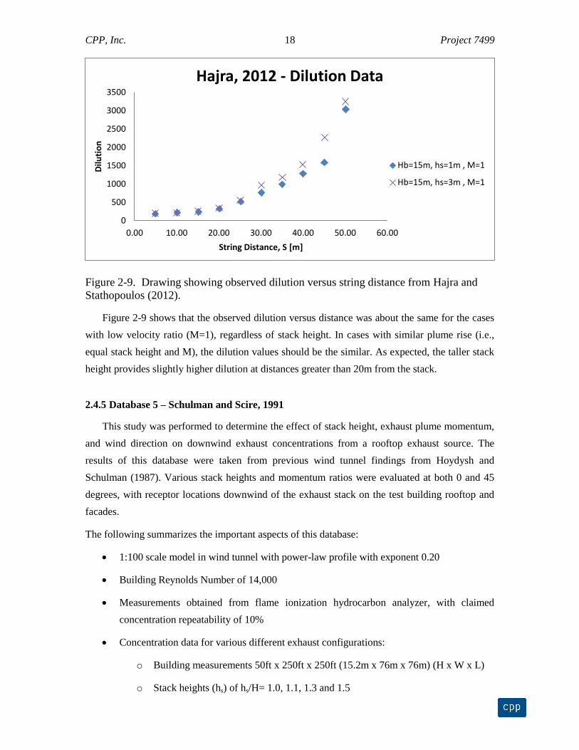
Figure 2-9. Drawing showing observed dilution versus string distance from Hajra and

Stathopoulos (2012).

Figure 2-9 shows that the observed dilution versus distance was about the same for the cases

with low velocity ratio (M=1), regardless of stack height. In cases with similar plume rise (i.e.,

equal stack height and M), the dilution values should be the similar. As expected, the taller stack

height provides slightly higher dilution at distances greater than 20m from the stack.

2.4.5 Database 5 – Schulman and Scire, 1991

This study was performed to determine the effect of stack height, exhaust plume momentum,

and wind direction on downwind exhaust concentrations from a rooftop exhaust source. The

results of this database were taken from previous wind tunnel findings from Hoydysh and

Schulman (1987). Various stack heights and momentum ratios were evaluated at both 0 and 45

degrees, with receptor locations downwind of the exhaust stack on the test building rooftop and

facades.


1:100 scale model in wind tunnel with power-law profile with exponent 0.20

Building Reynolds Number of 14,000

Measurements obtained from flame ionization hydrocarbon analyzer, with claimed

concentration repeatability of 10%


o Building measurements 50ft x 250ft x 250ft (15.2m x 76m x 76m) (H x W x L)

o Stack heights (hs) of hs/H= 1.0, 1.1, 1.3 and 1.5

0

500

1000

1500

2000

2500

3000

3500

0.00 10.00 20.00 30.00 40.00 50.00 60.00

Dilu

tio

n


Hajra, 2012 - Dilution Data

Hb=15m, hs=1m , M=1

Hb=15m, hs=3m , M=1


o Exhaust momentum ratios of (M= Ve/UH) of 1.0, 1.1, 3.0 and 5.0

o Receptors on rooftop and leeward walls, in direct line downwind of stack

o Wind azimuths of 0 and 45 deg

o Reference wind speed of 1.37 m/s (270 fpm)

For this study, only stack heights of hs/H = 1 and 1.1 were considered, as they are the stack

heights Standard 62.1 is most likely to be applied. Dilution values from this database were used

for azimuths of 0 deg and 45 deg at both rooftop and hidden receptors. The testing configuration

is illustrated below, in Figure 2-10.

Figure 2-10. Test building and rooftop receptor layout used for the Schulman and Scire Database

(1991).

Concentration measurement data was extracted from the database plots using a plot digitizer and

entered in tablature format into a spreadsheet. Plots of the measured dilution values versus string

distance for each configuration considered for this study are provided in Figure 2-11.


Figure 2-11. Drawing showing observed dilution versus string distance from Schulman

and Scire (1991).

The figure above shows a solid line as a “base-line case,” with each color representing a stack

height and azimuth. The various symbols are increases in exhaust stack momentum ratios. As

expected, increased dilution occurs with increased stack height and increases momentum ratio.

The abrupt increase in dilution represents a transition from a rooftop to hidden intake, and occurs

at approximately 40 m (131ft) for 0 deg azimuth, approximately 50 m (164ft) for 45 deg azimuth.

2.5 DILUTION EQUATION PERFORMANCE METRICS

When evaluating models for measurements and predictions pair in spaced and time, such as

for this evaluation, the following model performance measures are often used (Hanna et al.,

2004):

𝐹𝐵 = 2 [𝐷𝑜−𝐷𝑝

𝐷𝑜+𝐷𝑝] (2-1)

𝑀𝐺 = 𝑒𝑥𝑝[ln 𝐷0 − ln 𝐷𝑝] (2-2)

𝑁𝑀𝑆𝐸 = [[𝐷0−𝐷𝑝]

2

𝐷𝑜𝐷𝑝] (2-3)

𝑉𝐺 = 𝑒𝑥𝑝 [(ln 𝐷0 − ln 𝐷𝑝)2

] (2-4)

where


Dp: model prediction of dilution,

Do: observed dilution, and

overbar: average over the date set.

All four performance measures are calculated and considered together, since each measure

has pros and cons. For example, the linear measures FB and NMSE can be overly influenced by

infrequently occurring high observed and/or predicted concentrations, whereas the logarithmic

measures MH and VG may provide a more balanced treatment of extreme high values.

A perfect model would have FB, NMSE, MG, and VG = 0.0. For this evaluation, the

preferred model will have FB and MG ≤ 0 (predictions greater than observations) and the

smallest NMSE and VG. These statistics were initially used but were found to provide little

useful information since a conservative model is desired, or one that will under-predict dilution

most of the time. Hence, more relevant statistics were developed. The ratio, R, of predicted to

observed dilution was computed and percent time that the ratio met the following criteria was

computed.

% time R > 1.5 (percent time dilution predictions are a factor of 1.5 or more higher than

observed): the best model will have a low percentage.

0.5 ≤ % time R ≤ 1.5 (percent time dilution predictions are between a factor of 0.5 low to

1.5 high): the best model will have a high percentage.

0.5≤ % time R ≤ 1 (percent time dilution predictions are between a factor of 0.5 low to

perfect agreement): the best model will have a high percentage.

Another performance measure is a scatter plot of predicted divided by observed dilution (R)

with a one-to-one line. Again, the ideal model will have almost all predicted dilution values equal

to the observed dilution with a few values greater than observed and most values less than

observed. The goal is that the new equation over and underpredicts less than the current Standard

62.1 equation which would indicate that the new equation is more accurate.

2.6 EVALUATION OF STANDARD 62.1 EQUATION AGAINST DATABASES 1 AND 2

The following sections discuss the evaluation the Standard 62.1 equation against databases 1

and 2 (Wilson and Chiu, 1994 and Wilson and Lamb, 1994). The evaluation of the 62.1 equation

against all databases is discussed in Section 3.

Actual data from the Wilson and Chiu (1994) and Wilson and Lamb (1994) databases was not

obtained but the equations developed from those databases did bound the measured data and

provide a standard from which to evaluate the 62.1 equation discussed in Section 2.3. Figure 2-12

shows the predicted minimum dilution using the 62.1 equation (equation 2.7 in Section 2.3)


versus normalized string distance compared with predictions obtained using equations 2.1, 2.2

and 2.3 with Ve/UH (M) = 3.3 per Wilson and Lamb (1994) and using the following:

Set C1 = 7.0 and β1 = 0.0625 as recommended by Wilson and Chiu (1994);

Set C1 = 13.0 and β1 = 0.059 as recommended in ASHRAE, 1997); and

Set C1 = 13.0 and β1 = 0.04 as recommended by Wilson and Lamb, 1994.

These constants were found to bound all observed dilution values in Wilson and Lamb (1994)

and Wilson and Chiu (1991) and should be considered the most conservative. Inspection of

Figure 2-12 shows that all three previous minimum dilution equations produced similar results for

normalized distances, ξ, greater than about 20, while the Wilson and &Chiu (1994) equation

provided the lowed dilution estimates for ξ < 20

Figure 2-12. Predicted minimum dilution versus dimensionless sting distance using Standard

62.1 equation and other more accurate equations.


Figure 2-12 shows that the 62.1 equation is very conservative (underestimates minimum

dilution) for ξ <10 and tends to be non-conservative for ξ >10. This result confirms that the 62.1

equation needs improvement.

25

3. DEVELOPMENT AND EVALUATION OF NEW STANDARD 62.1 EQUATION

3.1 NEW EQUATION DEVELOPMENT

Four different minimum dilution equations are developed in the sections below followed by

and an evaluation of the equations against the Wilson and Chiu and Wilson and Lamb equations

discussed above and a comparison with predictions using the 62.1 equation.

3.1.1 New Equation 1 Development (New1)

A new general equation was developed using the method outlined below. First, start with the

basic Gaussian dispersion equation from the 2015 ASHRAE Handbook HVAC Applications

Chapter 45 (slightly modified) as follows:

)()(2

exp4

2

2

2ETTermlExponentiaxNETTermlExponentiaNon

h

dV

U = sD

z

p

ee

zyH

(3-1)

Next, the equation can be simplified using the following identities or approximations:

σy = σz ≈ (i2 s

2 + σo

2)

0.5

Qe = πVe de2/4

i = the average lateral (iy) and vertical turbulence (iz) intensity (assume the plume is

symmetrical for simplification purposes)

σo2 = de

2 (0.125 βM + 0.911 βM

2 +0.25), from ASHRAE 2007

Next, the non-exponential term (NET) can be written as:

𝑁𝐸𝑇 =𝜋𝑈𝐻

𝑄𝑒[𝑖2𝑠2 + 𝑑𝑒

2(0.125𝛽𝑀 + 0.911𝛽𝑀2 + 0.25)] (3-2)

which can also be written as,


𝑄𝑒(𝑖2𝑠2) +

4

𝑀𝑑𝑒2 𝑑𝑒

2(0.125𝛽𝑀 + 0.911𝛽𝑀2 + 0.25 ) (3-3a)

or simplifying,


𝑄𝑒𝑖2𝑠2 + 0.5𝛽 + 3.64𝛽𝑀 +

1

𝑀= 𝐴𝑠2 + 𝐵 (3-3b)

where

26

𝐴 =𝜋𝑖2𝑈𝐻

𝑄𝑒; 𝐵 = 0.5𝛽 + 3.64𝛽𝑀 +

1

𝑀 (3-4)

For a capped stack the B term above poses a problem since the M term is effectively 0, and B

would be become becomes undefined. Hence, for capped stacks B can be computed as follows.

𝐵 =0.785 𝑑𝑒

2𝑈𝐻

𝑄𝑒 (3-5)

The first term on left hand side is identical to equation 2.2 with 𝛽 = 0.071 instead 𝜋𝑖2.

Now consider the plume rise, ET, term:

𝐸𝑇 = 𝑒𝑥𝑝 (ℎ𝑝

2

2𝜎𝑧2) = 1 + (

ℎ𝑝2

2 𝜎𝑧2) +

1

2!(

ℎ𝑝2

2 𝜎𝑧2)

2

+1

3!(

ℎ𝑝2

2 𝜎𝑧2)

3

+ 𝐻𝑖𝑔ℎ𝑒𝑟 𝑂𝑟𝑑𝑒𝑟 𝑇𝑒𝑟𝑚s (3-6)

First, the plume rise needs to be approximated as follows:

ℎ𝑝 = ℎ𝑠 + ℎ𝑓 ≈ ℎ𝑠 + 𝜆 𝑑𝑒 𝑀 (3-7)

then

𝐸𝑇 = ≤ 1 + ({ℎ𝑠+𝜆 𝑑𝑒 𝑀}2

2 𝑖2𝑠2 ) (3-8)

which is still conservative (will underestimate dilution). An early approximation to final plume

(ASHRAE, 2007) had 𝜆 = 3.0 which will be the value used in this work.

Expanding,

𝐸𝑇 ≤ 1 + 1

2 𝑖2𝑠2{ℎ𝑠

2 + 2 𝜆 ℎ𝑠 𝑑𝑒 𝑀 + 𝜆2 𝑑𝑒2𝑀2} = 1 +

𝐶

𝑠2 (3-9)

where

𝐶 = 1

2 𝑖2{ℎ𝑠

2 + 2 𝜆 𝛽ℎ𝑠 𝑑𝑒 𝑀 + 𝜆2 𝛽𝑑𝑒2𝑀2} (3-10)

Combining the NET and ET terms results in

𝐷(𝑠) = (𝐴𝑠2 + 𝐵) (1 + 𝐶

𝑠2) = (𝐴𝑠2 + 𝐵 + 𝐴𝐶 +𝐵𝐶

𝑠2 ) (3-11)

𝐷𝑠2 = (𝐴𝑠4 + (𝐵 + 𝐴𝐶)𝑠2 + 𝐵𝐶 ) (3-12)

or

0 = (𝐴𝑠4 + (𝐵 + 𝐴𝐶 − 𝐷)𝑠2 + 𝐵𝐶 ) = 𝐴𝑠4 + (𝐸)𝑠2 + 𝐵𝐶 (3-13)

which is a form of the Quadratic Equation from which S can be solved for as follows:

27

𝑆21 =

−𝐸+ (𝐸2−4𝐴𝐵𝐶)0.5

2𝐴 𝑆2

2 = −𝐸− (𝐸2−4𝐴𝐵𝐶)

0.5

2𝐴 (3-14)

where

𝐸 = 𝐵 + 𝐴𝐶 − 𝐷 (3-15)

All dilution values between S1 and S2 will exceed the minimum dilution value and the safe

separation distances are outside that zone. New1 will compute minimum separation distances that

will account for all important variables (i.e., stack height, wind speed, exit velocity, and dilution

criteria).

New1 was then tested against the W&C and W&L equations and an “i” value of 0.153 was

determined that provided a best fit with W&C for 20<ξ,<1,000. Figure 3-1 shows that New1

dilution estimates versus those obtained using W&C and W&L with the graph from Wilson and

Lamb, 1994 alongside that includes the measured data. The figures show that New1 does provide

a lower bound for the observed dilution values for normalized distance, ξ, > 20 and also shows

that dilution starts to increase when you get closer to the stack. This is the effect of the plume

rise which was not included in the previous equations. However for ξ < 10, the New1 equation

might not be conservative since the measured dilution value at ξ ~ 10 appears to be lower than the

New1 prediction. Overall the results for New1 are encouraging but two alternate equations are

discussed below.

28

Figure 3-1. Comparison of New Equation 1 predictions versus Wilson and Chui and Wilson and

Lamb.

3.1.2 New Equation 2 Development (New2)

A 2nd

equation, New2, was developed in very similar manner as discussed in Section 3.1.1.

The only difference is that σo = 0.35 de as specified in ASHRAE (2011). With this definition,


𝑄𝑒[𝑖2𝑠2 + 0.123𝑑𝑒

2] (3-16)

or simplifying,


𝑄𝑒(𝑖2𝑠2) +

0.385𝑈𝐻𝑑𝑒2

𝑄𝑒= 𝐴𝑠2 + 𝐵 (3-17)

where “A” is the same as defined above and,

𝐵 =0.385 𝑑𝑒

2𝑈𝐻

𝑄𝑒 (3-18)

The ET term in section 3.1.1 does not change which means all equations are the same except for

“B” above.

Figure 3-2 below, again with i = 0.153 and λ = 3.0, shows New2 dilution estimates versus those

obtained using Wilson and Chui and Wilson and Lamb with the graph from Wilson and Lamb

alongside. The figure shows that New2 provides a better lower bound fit for all normalized

29

distances than New1 (see Figure 3.1). Based on this comparison, New2 is the preferred equation

for more detailed evaluation.

Figure 3-2. Comparison of New Equation 2 predictions versus Wilson and Chui and Wilson and

Lamb.

3.1.3 New Equation 3 Development

A 3rd

equation, New3, was developed in very similar manner as discussed in Section 3.1.2.

The only difference is in the exponential term, ET, where the vertical turbulence intensity, iz, is

used instead of i, as developed below.

𝐸𝑇 = ≤ 1 + (ℎ𝑠

2

2 𝑖𝑧2𝑠2) (3-19)

where iz is equal to 0.5 times the longitudinal turbulence intensity, ix, from Snyder (1981) Since i

= (iy+iz)/2 which from Snyder (1981) is equal to (0.75 ix + 0.5 iz)/2, it can be shown that iy = 0.8

i. Substituting into the equation above results in

𝐸𝑇 = ≤ 1 + ({ℎ𝑠+𝜆 𝑑𝑒 𝑀}2

2 (0.8 𝑖)2𝑠2 ) = ({ℎ𝑠+𝜆 𝑑𝑒 𝑀}2

1.28 𝑖2𝑠2 ) (3-20)

which means that C is now defined as:

30

𝐶 = 1

1.28 𝑖2{ℎ𝑠

2 + 2 𝜆 𝛽ℎ𝑠 𝑑𝑒 𝑀 + 𝜆2 𝛽𝑑𝑒2𝑀2} (3-21)

The NET term in section 3.1.2 does not change, which means all equations are the same except

for “C” above.

Figure 3.3 below, again with i = 0.153 and λ = 3.0, shows New3 dilution estimates versus those

obtained using Wilson and Chui and Wilson and Lamb with the graph from Wilson and Lamb

alongside. The figure shows that New3 provides a better lower bound fit for all normalized

distances than New1 (Figure 3.1) and similar agreement as New2 (Figure 3.2). Based on this

comparison and the fact that the vertical turbulence is accounted for more realistically, New3 was

initially considered the preferred equation for more detailed evaluation.

Figure 3.4 compares dilution estimates using all three equations and shows that New3 provides

dilution estimates that are in between New1 and New2 for small normalized distances. These

equations will be evaluated in more detail in the next Section.

Figure 3-3. Comparison of New3 predictions versus Wilson and Chui and Wilson and Lamb.

31

Figure 3-4. Comparison of New1, New2 and New3 predictions versus Wilson and Lamb.

3.1.4 New Equation 4 Development

A 4th equation, New4, was developed in very similar manner as discussed in Section

3.1.3. The only difference is that B is set equal to zero to add more simplification. Then

𝐿21 = 0 and 𝐿2

2 = −𝐸

𝐴= −

(𝐴𝐶−𝐷)

𝐴= −𝐶 +

𝐷

𝐴

where

𝐴 =0.0735𝑈𝐻

𝑄𝑒 (3-22)

𝐶 = 1

1.28 𝑖2{ℎ𝑠

2 + 2 𝜆 𝛽ℎ𝑠 𝑑𝑒 𝑀 + 𝜆2 𝛽𝑑𝑒2𝑀2} = 33.4{ℎ𝑠

2 + 6 𝛽ℎ𝑠 𝑑𝑒 𝑀 + 9 𝛽𝑑𝑒2𝑀2}

(3-23)

substituting

𝑀 = 4𝑄𝑒/(𝜋𝑑𝑒2𝑈𝐻) (3-24)

𝐶 = 33.37 {ℎ𝑠2 + 6 𝛽ℎ𝑠

𝑑𝑒 4𝑄𝑒

(𝜋𝑑𝑒2𝑈𝐻)

+ 9 𝛽𝑑𝑒2 [

4𝑄𝑒

(𝜋𝑑𝑒2𝑈𝐻)

]2

} (3-25)

32

Then

𝐿 = − 33.37 {ℎ𝑠2 + 24 𝛽ℎ𝑠

𝑄𝑒

(𝜋𝑑𝑒𝑈𝐻)+ 144 𝛽 [

𝑄𝑒

(𝜋𝑑𝑒𝑈𝐻)]

2} +

𝐷 𝑄𝑒

0.073 𝑈𝐻= − {33.37 ℎ𝑠

2 + 254.9 𝛽ℎ𝑠𝑄𝑒

(𝑑𝑒𝑈𝐻)+

486.9 𝛽 [𝑄𝑒

(𝑑𝑒𝑈𝐻)]

2} + 13.6 𝐷𝑄𝑒/𝑈𝐻 (3-26)

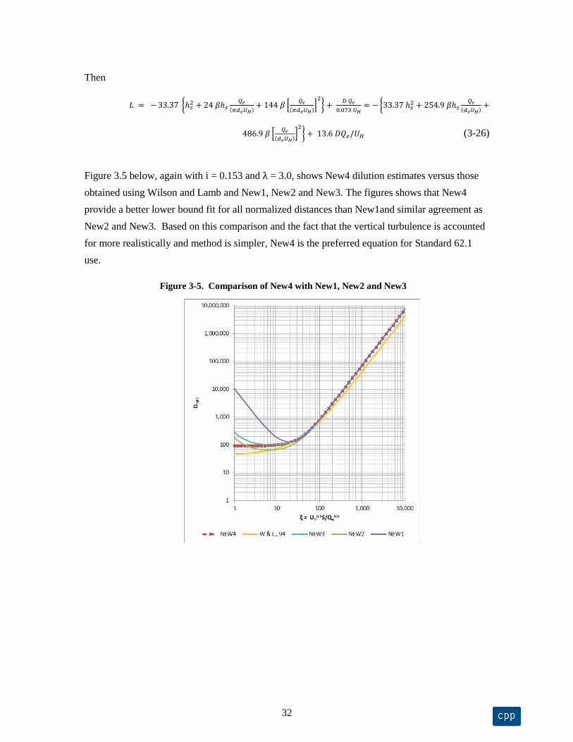
Figure 3.5 below, again with i = 0.153 and λ = 3.0, shows New4 dilution estimates versus those

obtained using Wilson and Lamb and New1, New2 and New3. The figures shows that New4

provide a better lower bound fit for all normalized distances than New1and similar agreement as

New2 and New3. Based on this comparison and the fact that the vertical turbulence is accounted

for more realistically and method is simpler, New4 is the preferred equation for Standard 62.1

use.

Figure 3-5. Comparison of New4 with New1, New2 and New3

33

4. EVALUATION OF 62.1 EQUATION AND NEW EQUATIONS

4.1 ASHRAE RESEARCH PROJECT (RP) 805 – 0 DEGREE WIND DIRECTION (PETERSEN, ET

AL., 1997)

Figure 4-1 shows scatter plots of predicted versus observed dilution for the existing Standard

62.1 equation and the New1, New2 and New4 equations. Note that a scatter plot for New3 is not

included as it was very similar to New2. The figure clearly shows that Standard 62.1 and New1

over predict dilution for certain cases (points shown above the solid black line), while New2 and

New4 provide overall better performance. Orange solid lines indicate predicted dilution +/- a

factor of 10 and the blue solid lines indicate +/- a factor of 3.

Table 4-1 shows the statistical quantities used to evaluate the model performance. The table

shows that New3 and New4 are an improvement over the current Standard 62.1 equation for the

following reasons:

smaller percentage of R values greater than 1.5 (less overprediction);

greater percentage of R values between 0.5 and 1.0 (less underprediction)

greater percentage of R values between 0.5 and 1.5 (more frequent predictions that

have a reasonable degree of uncertainty)

Table 4-1. Comparison of New Equation predictions versus ASHRAE RP 805 – 0 degree data.

Dp/Do = R Standard 62.1 New1 New2 New3 New4

% >1.5 3.9% 4.9% 0.5% 1.0% 0.3%

0.5<R<1 9.3% 15.1% 16.2% 16.4% 17.4%

0.5<R<1.5 17.5% 19.8% 17.5% 20.8% 20.8%

Yellow shading indicates best performance.

34


degree wind direction.

4.2 ASHRAE RESEARCH PROJECT 805 , 45 DEGREE WIND DIRECTION (PETERSEN, ET AL.,

1997)

Similar to Section 4.1, Table 4-2 and Figure 4-2 (below) compare predicted dilution values

for Standard 62.1 and the new equations. The data and metrics shown in this section reflect the 45

degree data taken from the ASHRAE RP 805 data set. It can be seen than the best prediction of

dilution come from the New2 and New4 equations for both the 0 degree and 45 degree data set.


shows that New2, New 3 and New4 are an improvement over the current Standard 62.1 equation

for the following reasons:

smaller percentage of R values greater than 1.5 (less overprediction);

greater percentage of R values between 0.5 and 1.0 (less underprediction)


have a reasonable degree of uncertainty).

35

Table 4-2. Comparison of New Equation predictions versus ASHRAE RP 805 – 45 degree data.


%>1.5 9.4% 17.9% 3.6% 7.6% 6.2%

0.5<R<1 8.0% 10.7% 12.9% 13.4% 12.5%

0.5<R<1.5 15.2% 19.6% 21.4% 22.8% 21.9%



degree wind direction.

The ASHRAE RP 805 database provided by far the most extensive data set, and was used as

the primary data set for the evaluation of the new equations. Based on inspection of Figure 4-1

and Figure 4-2, it can be seen that equations New2 and New4 provide the best predicted

concentrations, while conservatively bounding the dilution estimates. These equations are very

similar; however, equation New4 is theoretically sound and simpler to use, and is therefore

preferred for Standard 62.1 use. Equation New4 has been compared against several other data

sets, which are discussed in the following sections.

36

4.3 HAJRA AND STATHOPOULOS (2012)

Figure 4-3 shows scatter plots of predicted versus observed dilution for existing Standard

62.1 equation and the New1, New2 and New4 equations (New3 not shown as the result was

similar to New2). The orange solid lines indicate predicted dilution +/- a factor of 10 and the blue

solid lines indicate +/- a factor of 3.The figure shows that Standard 62.1 has fairly good

performance for this database and shows similar performance as the new methods. It should be

noted that for this database, a sub-set of the data was used, which included data for a low stack

height (1m, 3m) (3.28 ft, 9.84 ft) and low velocity ratio (M=1). Exhaust stacks with these

characteristics are of most interest in the implementation of Standard 62.1 and for which the

Standard 62.1 equation should perform the best, as it does.


shows that New 3 and New4 provide similar results as the current Standard 62.1 equation for the

following reasons:

same percentage of R values greater than 1.5 (minimal overprediction);

similar percentage of R values between 0.5 and 1.0 (similar underprediction)



Table 4-3. Comparison of Standard 62.1 and New3 predictions versus Hajra data – i=0.1527


>1.5 0.0% 0.0% 0.0% 0.0% 0.0%

0.5<R<1 50% 35% 40% 45% 45%

0.5<R<1.5 50% 40% 40% 60% 60%


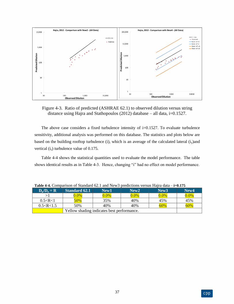
37

Figure 4-3. Ratio of predicted (ASHRAE 62.1) to observed dilution versus string

distance using Hajra and Stathopoulos (2012) database – all data, i=0.1527.

The above case considers a fixed turbulence intensity of i=0.1527. To evaluate turbulence

sensitivity, additional analysis was performed on this database. The statistics and plots below are

based on the building rooftop turbulence (i), which is an average of the calculated lateral (iy)and

vertical (iz) turbulence value of 0.175.


shows identical results as in Table 4-3. Hence, changing “i” had no effect on model performance.

Table 4-4. Comparison of Standard 62.1 and New3 predictions versus Hajra data – i=0.175


>1 0.0% 0.0% 0.0% 0.0% 0.0%

0.5<R<1 50% 35% 40% 45% 45%

0.5<R<1.5 50% 40% 40% 60% 60%


38

Figure 4-4. Ratio of predicted (ASHRAE 62.1) to observed dilution versus string

distance using Hajra and Stathopoulos (2012) database – all data, i=0.175.

Comparing Figure 4-3 and Figure 4-4, it can be seen that there is only a slight difference in

the predicted dilution values. Due to the slight variation that is observed, all databases were

evaluated with initially specified turbulence intensity of 0.1527.

4.4 SCHULMAN AND SCIRE (1991)

Figure 4-4 shows scatter plots of predicted versus observed dilution for existing Standard

62.1 equation and the New4 equation. The figure shows that New4 performs significantly better

than Standard 62.1. New4 predicts dilution more accurately, and provides a much better bound to

the data, and covers many more cases without over-predicting dilution. One case where New4

over-predicts dilution is for a case where the wind approaches the building at a 45 degree angle,

with the stack operating at a low velocity ratio (M). It should be noted that Standard 62.1 also

over-predicts dilution for this case. The over prediction in dilution results in a higher measured

39

exhaust concentration at the location, and may be due to building corner vortices and stack-tip

downwash. For such a case, Standard 62.1 over-predicts by nearly a factor of 10, while New4

over-predicts by approximately a factor of 3.


shows that New4 is an improvement over the current Standard 62.1 equation for the following

reasons:

much lower percentage of R values greater than 2.0 (significantly less

overprediction);

slightly lower percentage of R values between 0.5 and 1.0 (reasonable

underprediction); and

slightly lower percentage of R values between 0.5 and 1.5 (frequent predictions that


Table 4-5. Comparison of Standard 62.1 and New4 predictions versus Schulman data

Dp/Do = R Standard 62.1 New4

>2 33.1% 3.1%

0.5<R<1 25.2% 19.7%

0.5<R<1.5 32.3% 25.9%


Figure 4-5. Ratio of predicted (Standard 62.1) to observed dilution versus string distance

using Schulman and Scire (1991) database.

40

4.5 SIDEWALL (HIDDEN) INTAKES

Configurations when an intake is not in the line of sight of the exhaust should also be

considered. An example of such a configuration is a building with rooftop exhaust sources and

intakes located on the building façade. Such sidewall intakes are considered “hidden” from the

exhaust source. The 2015ASHRAE HVAC Application Handbook, Chapter 45, specifies that

dilution is enhanced by a least a factor two for a hidden intake which is discussed in more detail

in Section 6.3.3. Currently, Standard 62.1 does not have specific guidelines for such a case, other

than the slight benefit of increased “string distance.”

To account for hidden intakes, New4 dilution estimates are increased by a sidewall

concentration reduction factor of 2 (dilution increase factor), to account for the additional dilution

provided by the sidewall orientation. Table 4-6 and Figure 4-6 compare predicted values for

Standard 62.1 and New4 for cases where the intake is located along the building sidewall. The

two databases used for this evaluation are the ASHRAE RP 805 and the Schulman and Scire

(1991).


shows that New4 is an improvement over the current Standard 62.1 equation for the following

reasons:

equal or lower percentage of R values greater than 1.0 (less overprediction);

equal or greater percentage of R values between 0.5 and 1.0 (reasonable

underprediction); and

equal or greater percentage of R values between 0.1 and 1.0 (more frequent under

predictions that are within a factor of 10).

41

Table 4-6. Comparison of New Equation predictions versus ASHRAE Research Project 805 –

Hidden Intake Data

Dp/Do = R

ASHRAE Research Project

(Petersen, et.al. 1997) (Schulman and Scire, 1991)

Standard 62.1 New4 Standard 62.1 New4

> 1 0% 0% 33.3% 2.2%

0.5< R< 1.0 0% 0% 53.4% 55.6%

0.10 < R < 1.0 6.0% 8.3% 66.7% 97.8%


Figure 4-6. Comparison of New1, New2 and New4 predictions versus ASHRAE RP 805 and

Schulman - hidden intake data.

Figure 4-6 also shows that New4 with the factor of two sidewall dilution increase factor

generally provides better dilution predictions for sidewall receptors, with fewer predictions

varying greater than a factor of 10 from the measured dilution. In addition, based on the

Schulman database, Standard 62.1 has the potential to significantly over-predict dilution, which

can result in a potentially unsatisfactory design.

42

5. DEVELOPMENT OF REFINED DILUTION FACTORS

5.1 BACKGROUND AND OBJECTIVE

Table 5.1 provides a list of the minimum dilution factors provided in Standard 62.1 along

with the specified minimum separation distances. The table shows that dilution factors are only

provided for Class 3 and 4 exhaust, but the standard provides no basis for the criteria. Table 5.2

provides a summary of the minimum dilution factors from 62-1989R together with the minimum

separation distances. 62-1989R provides minimum dilution factors for Class 1 through 5 exhaust

but again no documentation was provided to support these factors. It should be noted that 62-

1989R provided no minimum separation distances for exhaust Classes 1-5 but the distances were

to be computed using the formula. This seems like a good approach since the distances will vary

with flow rate and exhaust velocity, and since the Standard 62.1 equation is rather simple.

Standard 62.1 just specifies one minimum distance for each exhaust class which is a problem as

discussed in Section 2.1 and demonstrated in Section 6.

Standard 62.1 provides the following definitions for the various air classifications.

Class 1: Air with low contaminant concentration, low sensory-irritation intensity, and

inoffensive odor.

Class 2: Air with moderate contaminant concentration, mild sensory-irritation

intensity, or mildly offensive odors. Class 2 air also includes air that is not

necessarily harmful or objectionable but that is inappropriate for transfer or

recirculation to spaces used for different purposes.

Class 3: Air with significant contaminant concentration, significant sensory-irritation

intensity, or offensive odor.

Class 4: Air with highly objectionable fumes or gases or with potentially dangerous

particles, bioaerosols, or gases, at concentrations high enough to be considered

harmful.

62-1989R provided similar definitions except for Class 4 and an added Class 5.

Class 4: Air drawn or vented from locations with noxious or toxic fumes or gases,

such as paint spray booths, garages, tunnels, kitchens (grease hood exhaust),

laboratories (filtered fume hood exhaust), chemical storage rooms, refrigerating

machinery rooms, natural gas and propane burning appliance vents, and soiled

laundry storage.

43

Class 5: Effluent of exhaust air having a high concentration of dangerous particles,

bioaerosols, or gases such as that from fuel burning appliance vents other than those

burning natural gas and propane, uncleaned fume hood exhaust, evaporative

condenser and cooling tower outlets (due to possible microbial contamination such as

Legionella the causative agent of Legionnaire’s Disease and Pontiac Fever).

Below is a typical listing of airstreams by class found in Standard 62.1-2013:

Class 1: arena, classroom, lecture hall, media center, computer lab, break room and

office space;

Class 2: auto repair room, locker room, kitchenettes, parking garage, toilet (private

and public), art class room, restaurant dining room, science laboratory, and

university/college laboratory;

Class 3: commercial kitchen hood other than grease, residential kitchen vented hood,

trash room, refrigerating machinery room, and daycare sickroom;

Class 4: commercial kitchen grease hood, paint spray booth, diazo printing

equipment discharge, chemical storage room, and laboratory hoods

Table 5.1 shows that plumbing vents have the same, or shorter, separation distance specified

as Class 2 air and hence will be treated as Class 2 air in this report.

Based on the above, the objective of this phase is to provide minimum dilution factors which

are based on sound scientific evidence, for many of the source types indicated in Table 5.1. The

following sections discuss the methodology and scientific evidence from which minimum

dilution factors are recommended.

44

Table 5-1 Minimum Separation Distances and Dilution Factors From Standard 62.1

5.2 GENERAL FACTORS TO CONSIDER

Developing minimum dilution factors (DF) is an important input for calculating minimum

separation distance, L. Dilution predictions by themselves are not useful for examining minimum

separation distances unless some minimum acceptable dilution, or design criterion, is specified.

This criterion will vary with source type and each source type may have a criterion that varies

depending upon such things as chemical utilization, chemical inventory, boiler or engine size, or

vehicle type or size. Standard 62.1-2013 currently defines only two minimum dilution factors: 15

for Class 3 exhaust and 50 for Class 4 exhaust. The method for obtaining the factors is not

described and, as shown below, are not reasonable for many sources with this classification.

An air quality “acceptability question” can be written:

𝐶𝑚𝑎𝑥,𝑝𝑟𝑒𝑑𝑖𝑐𝑡𝑒𝑑 < 𝐶ℎ𝑒𝑎𝑙𝑡ℎ,𝑜𝑑𝑜𝑟 (5-1)

where Cmax,predicted is the maximum predicted concentration at an air intake, Chealth is the health

limit concentration and Codor is the odor threshold concentration of any emitted chemical. When a

large number of potential chemicals are emitted from a pollutant source, it becomes operationally

ft mClass 2 air exhaust/relief outlet 10 3

Class 3 air exhaust/relief outlet 15 5 15

Class 4 air exhaust/relief outlet 30 10 50

Plumbing vents teminaing less than 3ft (1 m) above the level of the outdoor intake 10 3

Plumbing vents teminating at least 3ft (1 m) above the level of the outdoor intake 3 1

Vent, chimneys, and flues from combustion applicances and equipment (Note 3) 15 5

Garage entry, automobile loading area, or drive-in queue 15 5

Truck loading area or dock, bus parking/idling area 25 7.5

Driveway, street, or parking place 5 1.5

Thououghfare with high traffic volume 25 7.5

Roof, Landscaped grade, or other surface directl below intake 1 0.3

Garbage storage/pick-up area, dumpsters 15 5

Cooling tower intake or basin 15 5

Cooling tower exhaust 25 7.5

Minimum

Separation

Distance, L

Minimum

Dilution Factor,

DF

Object

ft m

Class 1 air exhaust/relief outlet Equation 5





ObjectMinimum Separation Distance, Minimum

Dilution Factor,

Table 5-2. Summary of Minimum Separation Distances and Dilution Criteria From Standard 62-

1989R. As indicated, an equation was used to calculate the minimum separation distance based on

the Minimum Dilution Factor. Distances were not specified.

45

simpler to recast the acceptability question by converting to dilution and then determining the

minimum dilution factor (DF) as follows:

𝐶𝑜 𝐶𝑚𝑎𝑥,𝑝𝑟𝑒𝑑𝑖𝑐𝑡𝑒𝑑⁄ > 𝐶𝑜 𝐶ℎ𝑒𝑎𝑙𝑡ℎ/𝑜𝑑𝑜𝑟⁄ = 𝐷𝑚𝑖𝑛(𝑝𝑟𝑒𝑑𝑖𝑐𝑡𝑒𝑑) > 𝐷𝑚𝑖𝑛,ℎ𝑒𝑎𝑙𝑡ℎ/𝑜𝑑𝑜𝑟 (5-2)

where

𝐷𝑚𝑖𝑛,ℎ𝑒𝑎𝑙𝑡ℎ/𝑜𝑑𝑜𝑟 = 𝑀𝑖𝑛𝑖𝑚𝑢𝑚 𝐷𝑖𝑙𝑢𝑡𝑖𝑜𝑛 𝐹𝑎𝑐𝑡𝑜𝑟 = 𝐷𝐹 (5-3)

The left side of Equation 5-2 is dependent on only external factors such as stack design,

receptor location, and atmospheric conditions. The right side of the equation is related to the

concentration of pollutant in exhaust stream and the health and/or odor threshold. Therefore,

highly toxic chemicals (small Chealth) with a low initial concentration may be of less concern than

a less toxic chemical with high initial concentration. The same holds true for odor thresholds.

Three pieces of information are needed to develop minimum dilution factors:

1) a list of the toxic or odorous substances that may be emitted, and

2) the health limits and odor thresholds for each emitted substance, and

3) the initial concentration of each substance in the exhaust stream.

It should be noted that the minimum dilution factors discussed below are derived from

occupational exposure limits, odor thresholds and estimated initial concentrations. The

occupational exposure limits are based on a mixture of guidelines, recommendations, and

regulatory limits from the ACGIH, OSHA or NIOSH. The limits provided by ACGIH and

NIOSH were developed as guidelines to assist in the control of health hazards, and are not

intended for use as legal standards. The limits provided by OSHA are regulatory limits on the

amount or concentration of an airborne substance that may be present in the workplace, and are

enforceable.

Defining minimum dilution factors for odors is often not simple. By itself, the concentration

of an odorous substance in air is not necessarily an indicator of the corresponding human

response. Other factors include the detection threshold, intensity (perceived strength), character

(sweet, grassy, etc.) and hedonic tone (offensiveness) of an odorant (ANSI/ASHRAE 2013).

Reviews of odor measurement techniques, and the factors that influence odor annoyance

thresholds, are available in Pullen (2007) and ANSI/ASHRAE (2013). In this report, we are

concerned with odor concentration only, and leave aside factors such as the frequency and

duration of an offending odor.

46

Below, we discuss dilution factors for odors that are typically unpleasant in hedonic tone (i.e.,

sense pleasure or displeasure), such as diesel or toilet odors, and odors that may be unpleasant

when out of context, such as kitchen odors that infiltrate an office space. Amoore (1985) provides

a “provisional rule” that an unpleasant odor will be at its annoyance threshold for 50% of people

when the concentration of the odorant is at 5 times its detectable level (i.e., 5 odor units (OU)).

This is also cited by Mahin (2001) who provides a table of off-site odor standards and guidelines

from around the world. We adopt this rule in our analysis when no other values were available.

Standards for U.S. locations are shown in Table 5.3 below.

The detection threshold of an odorant is typically defined as the concentration at which 50%

of people (often trained odor judges) are able to detect, though not necessarily identify, an odor.

Concentrations of odorants in air are sometimes given in units typically used in air quality, such

as ppmv, ppbv or μg/m3. However, these units are not easily applied to odorants comprising

chemical mixtures; therefore odorant concentration is often expressed in odor units (OU) (Nicell

2003). An odor unit signifies the number of dilutions, by non-odorous air, of a pure odorant until

it is at the detection threshold (ANSI/ASHRAE 2013, Pullen 2007, Nicell 2003). In other words,

an odorant concentration of 50 OU (or, equivalently, 50 OU/m3 in Europe) is at 50 times its

detection threshold. Equivalently, 50 dilutions-to-threshold (D/T) are needed to render the

odorant undetectable by 50% of people. These units are used interchangeably here.

The following paragraphs discuss the specific minimum dilution factors for different source

types.

5.3 RECOMMENDED DILUTION FACTORS

5.3.1 Combustion Type Sources

5.3.1.1 General

Health limits for combustion type sources are primarily related to the release of CO, NOx,

SO2 and particulate matter (PM). These chemicals may also be limiting for defining an odor

threshold for combustion equipment using natural gas; however, for diesel exhaust, the limiting

odor is a caused by a complex mixture of various chemicals and particulates.

Objection levels to various dilutions were obtained from Vanderheyden (1994) and

Cernansky (1983). Dilutions that produced a 20 percent objection level were used to quantify the

odor occurrences. At the 20 percent objection level, Vanderheyden (1994) indicates a dilution of

1:2000 is necessary to avoid odors. In an unpublished study by CPP of exhaust from a 2.5 MW

47

diesel generator, odor panel results gave a mean odor detection threshold of 2,830, which agrees

fairly well with the 1:2000 dilution value of Vanderheyden (1994).

After-market filters are available for some diesel combustion sources. These filters typically

reduce unburned hydrocarbons (the odorous exhaust components), by about 80%. If these filters

are installed, the 1:2000 dilution requirement stated above is reduced to a 1:400 dilution

requirement.

Table 5-3 provides a summary of the health and odor limits used to determine minimum

dilution factors for combustion type sources. National Ambient Air Quality Standards (NAAQS)

are also provided in the table for reference purposes but are only applicable at the property line

and beyond and will not be used to set minimum dilution factors. It should be noted that Table 5-

3 is not all inclusive as other countries and states have different standards or thresholds (e.g., for

CO, Health Canada has a 25 ppm threshold and California has a 20 ppm threshold; for NO2 the

California limit is 30 ppb).

To determine the minimum dilution factors, the initial concentrations of the pollutants in the

exhaust streams are needed and can be computed from emission rates often provided by the

manufacturer. For this evaluation, emission rates were obtained from EPA’s AP-42 Compilation

of Air Pollutant Emission Factors, Volume I, Stationary Sources Point and Area Sources (1995)

or from the Code of Federal Regulations (CFR, 2002).

Emission factors are provided for NOX but a conversion factor is needed to estimate the

Table 5-3. Health and Odor Thresholds for Combustion Equipment

Pollutant NAAQS (1-hr)2

Odor NAAQS Reference Odor Reference

(µg/m³) TWA STEL (µg/m³)

Combined Exhaust (dilution): 2,000Vanderheyden, M.D., D.S. Chadder, and A.E. Davies, “A

Novel Methodology for Predicting the Impact of Model

Sources on Air Quality,” presented at the 87th Annual Meeting

of the Air & Waste Management Association, June 1994.

CO - ACGIH(1) 43,200 NA 229,000

76 FR 54294, Aug 31,2011,

35 ppm 1-hour, once per year

NO - NIOSH(1) 30,000 90,000 657 Ruth, 1986, geometric mean of range 0.36 and 1.2 mg/m3

NO2 - NIOSH (1) 188 1,800 332

75 FR 6474, Feb 9, 2010,

100 ppb, 98th percentile of 1-

hr daily maximum

concentrations, average over 3

years

AIHA, Odor Thresholds, 2013, geometric mean of range

0.058 - 0.5 ppm (0.11-1.0 mg/m3)

SO2 - ACGIH(1) 196.5 13,000.0 3,755

75 FR 35520, June 22, 2010,

75 ppb 99th percentile of 1-

hour daily maximum

concentrations, average over 3

years

AIHA, Odor Thresholds, 2013,, gemometric mean of range

range of 0.33 - 8 ppm (0.87 - 21 mg/m3)

PM10 OSHA(1) 375.0 15,000.0 45,000.0

40 CFR part 50, 24 average

of 150 scaled to 1-hr using

0.4 scaling factor

PM2.5 OSHA(1) 88 5,000 15,000

40 CFR part 50, 24 average

of 35 scaled to 1-hr using 0.4

scaling factor

1) Only applies to Health Limits.

2) National Ambient Air Quality Standards (NAAQS) only apply off-site (at the property line and beyond)

Health (µg/m³)

48

emission rates for nitric oxide (NO) and nitrogen dioxide (NO2). For this study, a 75% conversion

factor was used to convert NOx to NO2 and a 25% conversion factor was used to convert NOx to

NO.

5.3.1.2 Diesel generators and diesel vehicles

For diesel generators and diesel vehicles, health and odor criteria based on chemical emission

rates are not limiting with regard to a minimum dilution factor, rather the odor due to the exhaust

mixture is limiting as discussed above. The recommended dilution factor is 2000 for unfiltered

diesel exhaust. If an 80% efficient odor filter is used, either on the exhaust or on the intake, the

minimum dilution factor would be 400. If a 90% efficient odor filter is used, either on the exhaust

or intake, the dilution factor would be 200.

5.3.1.3 Light duty gas vehicles

Table 5.4 shows the calculation of the minimum dilution factor for a single idling light duty

gas vehicle and for multiple idling gas vehicles. For both cases, the dilution factor is 47 (the

recommended value is 50). The single idling vehicle dilution factor is appropriate for garage

entry, automobile loading area or drive-in queue intake separation distance calculations. The

multiple idling vehicle case is provided so that criteria can be developed for parking garage

exhaust vents. If the exhaust vent flow is increased, the dilution criterion is computed as follows:

DFnew = DF * n where n is equal to the maximum number of vehicles idling times the exhaust

flow per vehicle divided by the fan exhaust flow. According to the California Mechanical Code,

the exhaust flow per active vehicle is 14,000 cfm (6.6 m3/s). Table 5.4 provides an example

calculation based on this exhaust flow per active vehicle. The table shows that very little

additional dilution is needed (i.e., a dilution target value of 0.3).

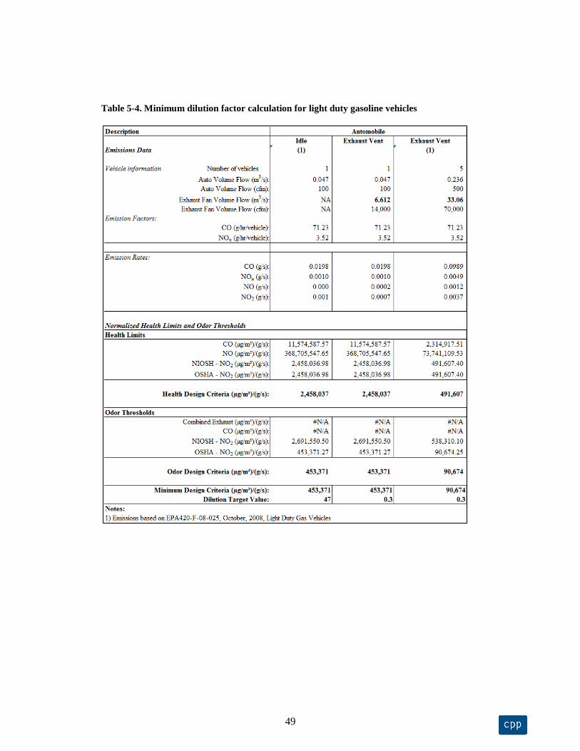
49

Table 5-4. Minimum dilution factor calculation for light duty gasoline vehicles

50

5.3.1.4 Boilers

Table 5.5 below shows the calculation of minimum dilution factor for boiler exhaust based on

the discussion in Section 5.3.1. Based on Table 5.5 the following equation can be used for

calculating the minimum dilution factor: DF = 2.8 x ppm NOx. For example, a boiler exhaust

with 10 ppm NOx would have a minimum dilution factor of 28.

Table 5-5. Calculation of Dilution Targets for Boiler Exhaust.

51

5.3.2 Kitchen

Commercial kitchen grease exhaust is regarded as Class 4 air (non-grease exhaust is regarded

as Class 3 air) in ANSI/ASHRAE Standard 62.1 (ANSI/ASHRAE, 2013). Section 5 of the

standard requires a minimum separation distance of 30 ft (10 m) between exhaust and any air

intakes, or 50 dilutions (see Table 5-1), for Class 4 air. Generally, health effects are not

considered for Kitchen exhaust as there are no published chemical emissions rates.

Abundant research exists on the composition and nature of odors and aromas resulting from

food production (e.g., Belitz 2009, Nicolay 2006, Grosch 2001), but much of it is not

immediately applicable to the definition of kitchen odor thresholds or dilution requirements. This

is due in part to the chemical nature of food aromas and odors, which comprise multiple

chemicals that have synergistic effects on human olfactory systems (Nicolay 2006). In other

words, odors produced by chemical mixtures may produce odor characteristics that are not

indicative of any single component. For example, methanethiol is a key odorant of flatus (see

section 5.3.4), but is also a key odorant in the aroma of french fries (Wagner 1998) and boiled

beef (Grosch 2001). An additional complication is that, like all odors, food odors have different

hedonic tones (levels of pleasantness or offensiveness) that influence the threshold at which an

odor becomes annoying. Fresh baked bread, for example, is given a hedonic score of 3.53 on

Dravnieks’ scale (the most pleasant odor being 4), while the odor of eggs is near neutral at 0.45,

and sauerkraut is slightly unpleasant with a score of -0.60 (Dravnieks, et al. 1984).

Unfortunately, there is a paucity of published data defining odor thresholds for typical

commercial restaurants. However, odor analysis of the exhaust from two restaurants, each

belonging to a different well-known fast-food chain, was performed by the IVL Swedish

Environmental Research Institute in the context of analyzing an air purification system (Peterson

2011, 2008). Bagged exhaust samples were taken from the rooftop ductwork of the restaurants

and analyzed by odor panels comprising trained members. Depending on sampling location

(within the duct work) and time of day, odor concentrations based on detection (not recognition)

in untreated exhaust ranged from about 1,500 to almost 3,400 OU/m3 between the two

restaurants.

Although the exhausts from only two different restaurants were sampled, we assume that

these are representative of the type of kitchen grease exhaust that is likely to initiate odor

complaints. In addition, the odor concentrations reported in above are of the same order and range

as unpublished data, obtained by CPP, indicating odor detection thresholds of 850 OU for a grill

exhaust, and 3,200 OU for a rotisserie exhaust, of a wood burning restaurant kitchen.

52

Assuming an annoyance threshold of 5 OU (Amoore 1985), and ignoring issues of hedonic

tone, the range of odor thresholds derived from Peterson (2011, 2008) results in a corresponding

range of about 300 to 700 dilutions to decrease the odor concentration of commercial kitchen

exhaust below the level of annoyance. Although much greater than the ANSI/ASHRAE standard

of 50 dilutions (62.1, 2013, Appendix F), these values accord with CPP’s experience regarding

effective dilutions for kitchen grease exhaust.

Based on these results, a 300 dilution factor will be recommended for commercial kitchen

exhaust and a dilution factor of 700 for wood burning kitchen exhaust.

5.3.3 Cooling Tower

The minimum dilution factor for cooling tower exhaust is based estimated emission rates for

various chemicals that are used to reduce and/or eliminate algae, bacterial and fungal growth as

well as reduced corrosion of equipment. These chemicals are also used to help avoid Legionella

(EPA, 1999). Vanderheyden and Schulyer, 1994 evaluated various chemicals in the cooling

towers exhaust and found that the worst case chemical was glutaraldehydes with an initial exhaust

concentration range of 140 to 4320 ug/m3 was observed. The NIOSH recommended exposure

limit (REL) is 800 ug/m3 and the ACHIH TLV is 200 ug/m3 which gives a dilution range of

about 5 to 20 using the highest observed initial exhaust concentration. Based on the range dilution

range of 5 to 20, a reasonable recommended value is 10.

5.3.4 Toilet

Exhaust from public and private toilets is regarded as class 2 air in ASHRAE standard 62.1-

2013. Such emissions are generally not harmful, but may be a source of odor annoyance or

nuisance if the exhaust is re-entrained into fresh air intakes that service areas used or other

purposes. The minimum separation distance between a single toilet exhaust and any outdoor air

intake is 10 ft (3 m) for class 2 air (ASHRAE 62.1).

There are several sources of odor that may be emitted from toilets and bathrooms, including

those of cleaning products, but human flatus is most often the cause of objectionable odors. Three

volatile sulfur compounds (VSCs)—hydrogen sulfide, methanethiol (methyl mercaptan) and

dimethyl sulfide—are largely responsible for odor arising from human feces and flatus

(Tangerman 2009, Suarez et al. 1998). Suarez et al. (1998) identified hydrogen sulfide as the

primary correlate for the odor of human flatus, but Tangerman (2009) notes that pinto beans were

added to the diets of the subjects in the Suarez et al. study, which may have influenced the

hydrogen sulfide content of the flatus. Measured concentrations of hydrogen sulfide differed

53

greatly between the Suarez and Tangerman studies, with mean values of 25.4 (±4.8) ppmv and

3.6 (±1.3) ppmv, respectively. In addition to this difference, Tangerman (2009) notes that

methanethiol has a stronger foul odor than hydrogen sulfide even when the concentration of

hydrogen sulfide is five times higher than that of methanethiol. Based on this and other evidence,

he concludes that methanethiol is mainly responsible for the objectionable odor of human flatus.

We assume that this conclusion is correct in the following analysis.

Odor thresholds of methanethiol reported in the literature range over several orders of

magnitude, from 0.01 ppbv to 42 ppbv. This range may reflect differences in the training, age and

natural sensitivities of odor panel members, as well as vagueness in the definition of an odor

threshold. There may also be confusion between reported perception thresholds, in which a smell

is merely perceived, and recognition thresholds, in which more than half of odor panel members

can identify the odor. Tangerman (2009) reports that the odor of methanethiol is perceivable at a

concentration of only 0.01 ppbv, and objectionable at 12 ppbv, though it is not clear how

“objectionable” is defined. The NRC (2013) predicts a “level of awareness” (i.e., a level at which

more than half of people will perceive “a distinct odor intensity”) of 1.9 ppbv for methanethiol.

Reported thresholds are given in Table 5-6. Note that the median of these threshold values (0.111

ppbv) is less influenced by the outlying values and is close to the value given by Van Doorn

(2002, as cited in NRC 2013). In the analysis below, we assume an annoyance threshold of five

times the detection threshold (Mahin 2001, Amoore 1985).

The volume of gas passed by healthy humans varies from 400 to 2400 ml per day and

emissions occur about 14 (±4) times per day (Levitt and Bond 1980). Suarez et al. (1998) report

Threshold (ppbv) Reference Cited in

41 Katz and Talbert 1930

0.990 Wilby 1969

0.015 Williams 1977

0.120 Van Doorn 2002

19 Nishida et al. 1979

0.102 Van Harreveld 2003

0.070 Nagata 2003

0.500 WEF 1995

0.010 Tangerman 2009 Tangerman 2009

0.020 Ruth 1986 (low value) Ruth 1986

NRC 2013

Pullen 2007

Table 5-6. Odor detection thresholds reported for methanethiol.

54

an average flatus emission volume of 107 (±8.1) ml, while Tangerman (2009) reports a somewhat

lower value of 84 (±16) ml. Average concentrations of methanethiol in flatus were statistically

identical in both studies, with values of 5.04 (±0.960) ppmv and 5.18 (±1.06) ppmv in Suarez et

al. (1998) and Tangerman (2009), respectively. Here, we assume an average emission volume of

100 ml with a methanethiol concentration of 5 ppmv per emission.

To estimate external dilutions required for restroom exhaust, we multiply the assumed

emission volume by a typical “safety factor” of five to give an emission volume of 500 ml per

stall. Though toilet stalls are obviously not airtight, the dimensions of a typical, non-ADA toilet

stall (3 ft x 5 ft x 6 ft) provide a reasonable volume scale (90 ft3 or 2.6 m

3) with which to estimate

dilution within the restroom space, and by which to normalize dilutions on a ‘per stall’ basis.

Table 5-7 provides estimates of interior dilutions, and the corresponding exhaust dilutions

required to obtain the annoyance threshold, based on the high and low annoyance threshold

values found in the studies referenced above. This calculation assumes the ASHRAE standard

(2013) ventilation rate of 70 CFM (0.033 m3/s) per urinal or water closet.

The minimum threshold value, combined with our assumptions of emission volume,

concentration and interior dilution volume, provides an upper limit of 20 exterior dilutions to

decrease the methanethiol concentration to an acceptable level (Table 5-7). However, the

geometric mean threshold value results in only 5.8 exterior dilutions, and, based on CPP’s

experience with restroom exhausts, is likely to be the most realistic value. Based on these results,

the 62-1989R Class 2 recommended dilution factor of 10 seems appropriate for toilet exhaust

which is classified as Class 2 exhaust in Standard 62.1 (2013).

5.4 SUMMARY OF RECOMMENDED VALUES AND DISCUSSION

Table 5-8 below provides a summary of the recommended minimum dilution factors for the

source types investigated as part of this research. The following discussion provides the basis for

the recommendations.

Table 5-7. Summary of Toilet Exhaust Odor Study Results

55

Class 1. This exhaust type is normally room air with minimal odors and no

hazardous air pollutants and therefore very little dilution of the exhaust stream is

needed. Standard 672-1989R specified minimum dilution factor of 5 which still

seems adequate, if not somewhat conservative.

Class 2. Of all the exhaust steams with this classification, toilet exhaust seems to be

the most potentially offensive one from an odor perspective. The recommended DF

value for this exhaust per the discussion in Section 5.3.4 is 10 which is the

recommended value and is the same value specified in Standard 61.1 (2013).

Class 3. No additional documentation was found regarding the appropriate dilution

factor for Class 3 exhaust. A reasonable assumption is to use the geometric mean

between the Class 2 and Class 4 dilution factors which are fairly well documented.

The geometric mean is approximately 50 and is the recommended value.

Class 4. The documentation for a minimum dilution factor of 300 for commercial

kitchen exhaust is fairly well documented as discussed in Section 0.

Table 5-8. Summary of Recommended Minimum Dilution Factors, DF

56

6. UPDATED SEPARATION DISTANCE METHODOLOGY

6.1 CALCULATED SEPARATION DISTANCES (GENERAL AND REGULATORY PROCEDURE)

The stated purpose of this research project is to provide a simple, yet accurate procedure for


outdoor air intake to a ventilation system to avoid re-entrainment of exhaust gases. Two new

procedures were originally thought to be needed. One a general procedure suitable for standard

HVAC engineering practice that has as independent variables: exhaust outlet velocity; exhaust air

volumetric flow rate; exhaust outlet configuration (capped/uncapped) and position (vertical

separation distance); desired dilution ratio; ambient wind speed; and exhaust direction. The

second method was to be a regulatory procedure suitable for Standard 62.1, Standard 62.2, and

model building codes that has as independent variables only exhaust outlet velocity, exhaust air

volumetric flow rate, desired dilution ratio, and a simple way to account for orientation relative to

the inlet. The recommended equation (New4), with the addition of “special cases” discussed in

the next section, meets both requirements. New4 accounts for all the important variables, yet is

simple enough to be used as a regulatory method.

The methodology for computing minimum separation distances using New4 along with

example calculations and additional documentation is found in the following sections.

6.2 GENERAL EQUATION AND METHOD

To compute the minimum separation distance, L, the following methodology should be

utilized, where L replaces S from Section 3. First, setup a spreadsheet as shown in Table 6-1.

Next, the values in yellow are input, and all other values are computed using the equations below.

The details on the special cases (i.e., horizontal exhaust pointed away from intake, upblast

exhaust, heated exhaust, hidden intake, and heated capped or louvered exhaust) are discussed in

Section 6.3.

The equations and method are provided below.

𝐹1 = 13.6𝐷𝑄𝑒

𝑈𝐻; (6-1)

𝐹2 = 33.37 ℎ𝑠2 + 254.9 𝛽

𝐵𝑓𝑎𝑐ℎ𝑠𝑄𝑒

𝑑𝑒𝑈𝐻+ 486.9 𝛽 [

𝐵𝑓𝑎𝑐𝑄𝑒

𝑑𝑒𝑈𝐻]

2 (6-2)

57

𝐵𝑓𝑎𝑐 = [1 + ( 1180800 (𝑇𝑠−𝑇𝑎)𝑇𝑠

𝑇𝑎2𝑈𝐻𝑉𝑒

)]0.5

(𝑆𝐼) (6-3)

𝐵𝑓𝑎𝑐 = [1 + ( 30.5 (𝑇𝑠−𝑇𝑎)𝑇𝑠


)]0.5

(I-P) (6-4)

𝐹𝑖𝑛𝑑 𝑚𝑎𝑥𝑖𝑚𝑢𝑚 𝑜𝑓 [𝐹1 − 𝐹2] 𝑏𝑦 𝑣𝑎𝑟𝑦𝑖𝑛𝑔 𝑈𝐻 𝑏𝑒𝑡𝑤𝑒𝑒𝑛 1.5 𝑚 𝑠⁄ 𝑎𝑛𝑑 10 𝑚 𝑠⁄

𝑖𝑓 𝑚𝑎𝑥[𝐹1 − 𝐹2] > 0; 𝐿 = [𝐹1 − 𝐹2]0.5 (6-5)

𝑖𝑓 𝑚𝑎𝑥[𝐹1 − 𝐹2] ≤ 0; 𝐿 = 0

where:

L = minimum separation (stretched string as shown in Figure 6-1) distance (m, ft);

UH = wind speed at stack top (m/s; fpm);

D = dilution factor (taken from Table 5-8);

Ts = exhaust temperature (K; R);

Ta = ambient temperature (K; R);

hs = stack height above the top the air intake (m; ft);

Qe = exhaust air volume flow rate (m3/s; cfm); for gravity vents, such as plumbing vents,

use an exhaust rate of 150 cfm (75 L/s); for flue vents from fuel-burning appliances,

assume a value of 250 cfm per million Btu/h (0.43 L/s per kW) of combustion input (or

obtain actual rates from the combustion appliance manufacturer;

de = exhaust diameter (m; ft); for rectangular exhaust (capped, horizontal or vertical), an

equivalent round stack diameter should be calculated using the following equation:

de,,eff = [Exhaust Area x 4/π]0.5

for louvered round or rectangular exhaust (capped, horizontal or vertical), an equivalent

round stack diameter should be calculated as follows:

de,eff = [Exhaust Area x Open Fraction x 4/π]0.5

;

for heated capped or horizontal (including louvered) exhaust, the exhaust diameter is the

actual or effective diameter multiplied by 10 as discussed in Section 6.3.5;

β = 1 for uncapped stacks and 0 for capped or horizontal (includes louvered) exhaust;

Section 6.3.1 discusses the method to treat horizontal exhaust pointed away from the

intake; for heated capped or horizontal exhaust, β = 1 and de and Qe are computed as

discussed in Section 6.3.5.

58

The following describes the calculations and information that is input into Table 6.1.

Row 1: The exhaust type first needs to be specified from Table 5-8 and then the

appropriate dilution factor from the table is input. For Class 1 exhaust, the

dilution factor is 5 which is the value in the table.

Row 2: If the intake is on a building sidewall or on the opposite side of a roof top

obstacle (hidden), the dilution factor can be decreased by a factor of 2 which is

then input into the table. If the intake is not hidden, the value should be set to 1.

More details are found in Section 6.3.3.

Row 3: If the exhaust is horizontal and pointed away from the intake as described in

Section 6.3.1, the dilution factor can decreased by an additional factor of 1.7 and

that value is input into the table. For all other cases, a value of 1 is input.

Row 4: The final dilution factor is computed by dividing the dilution factor in Row 1 by

the factors in Rows 2 and 3.

Row 5: The height of the stack above the top of the intake is input. For intakes on a

building sidewall or behind a roof-top obstacle, the height of the stack above the

roof or obstacle top where the intake is located should be used. If the intake, is

above the stack height, the height difference is negative and the stack height

input is also negative.

Row 6: For capped or horizontal exhaust (including louvered), a value of zero is entered;

For all other exhaust types including heated capped or horizontal exhaust pointed

away from the input, the value should be 1.0.

Row 7: The exhaust diameter is entered using the methods described above.

Row 8: The exhaust volume flow rate is entered.

Row 9: The exhaust temperature is entered. Unless the exhaust is heated, this

temperature should be the same as the ambient temperature.

Row 10: Enter the ambient temperature. A default value of 21.1 C (70 F) should typically

be used.

Row 11: The heated exhaust factor is computed using Equation 6-4 as discussed in detail

in Section 6.3.4.

Row 12: The exhaust velocity is computed using the equation in the table.

Row 13: F1 is computed using Equation 6-1.

Row 14: F2 is computed using Equation 6-2.

Row 15: For non-capped or heated horizontal exhaust and heated capped exhaust, the

wind speed is varied between 1.5 and 10 m/s (300 and 2000 fpm) and the

difference between F1 and F2 is maximized. If the maximum value is negative,

59

the minimum separation distance is zero. If the difference is positive, then the

initial separation distance is computed using Equation 6-5. For capped stacks or

horizontal exhaust not pointed away from the intake, a wind speed of 1.5 m/s

should be used. For horizontal exhaust pointed away from the intake the wind

speed should be set equal to the exit velocity (see Section 6.3.1).

Row 16: F1-F2 is computed.

Row 17: Linitial is computed using Equation 6.5

Row 18: Lfinal is the same as Linitial for all exhaust except horizontal exhaust that is

pointed away. For the latter case, Lfinal is computed using the equation in the

table as discussed in Section 6.3.1.

Figure 6-1. Diagram showing how to calculate string distance, L. In the figure L = L1+L2+L3

60

Table 6-1 Example Spreadsheet for Use in Calculating Separation Distances

61

6.3 SPECIAL CASES

6.3.1 Horizontal Exhaust

When an exhaust is pointed away from an intake and the wind is blowing toward the intake,

the exhaust travels some direction upwind and then turns around. The upwind distance traveled

depends upon the ratio of exhaust velocity to wind speed (velocity ratio). The plume is also

diluted as it travels upwind. For small velocity ratios, the exhaust turns around quickly (within

0.5de for a velocity ratio of 0.5) and for high velocity ratios, the plume travels upwind for a larger

distance (6de for a velocity ratio of 5). An integral plume model (Petersen, 1987) was used to

estimate the dilution and travel distance versus velocity ratio. From this analysis, the following

rules were developed when an exhaust is pointed away from an intake.

“Pointed away” includes cases where the direction of the exhaust is oriented 180

degrees away from the intake ± 45 degrees;

Set UH = Ve ;

Decrease the minimum dilution factor by a 1.7;

Decrease the separation distance by 1.75 de.

6.3.2 Upblast and Downblast Exhaust

For upblast exhaust (typically used for Kitchen exhaust), the effective exhaust velocity is

computed using the dimension “A” for de in the figure below and the exhaust volume flow rate

along with the following equation:

𝑉𝑒 = 𝑄𝑒

(𝜋𝑑𝑒2/4)⁄ (6-6)

Figure 6-2 Typical Upblast Exhaust

62

Downblast exhaust (e.g. “mushroom” exhausters) are treated the same as a capped exhaust

stack and input exhaust diameter is “A” in the figure above. If the downblast stack is heated, the

method in Section 6.3.5 can be used.

6.3.3 Hidden Intakes

A hidden intake is defined as one that cannot be seen if standing at the exhaust location.

Typically, hidden intakes are on building sidewalls or on the side of a large mechanical penthouse

or unit. The 2015ASHRAE HVAC Application Handbook, Chapter 45, specifies that dilution is

enhanced by a least a factor two for a hidden intake. Hence, for hidden intakes the minimum

Dilution Factors in Table 5-8 are divided 2.0. It should be noted that a hidden intake should meet

one of the following criteria: 1) be off the same roof as the exhaust and on a building sidewall; 2)

be on the same roof as the exhaust but on the other side of a significant obstruction.

A significant obstruction is defined as one that would increase the size the plume by at least a

factor of two which would result in a dilution increase of at least a factor of two. The minimum

obstruction height and width can estimated using initial plume spread estimates (σyo and σzo)

defined as follows:

𝜎𝑦𝑜 =𝑊

4.3; 𝜎𝑧𝑜 =

𝐻

2.15 (6-7)

The dilution increase can be used using the following equation:

𝐷𝑖𝑙𝑢𝑡𝑖𝑜𝑛 𝐼𝑛𝑐𝑟𝑒𝑎𝑠𝑒 𝑓𝑎𝑐𝑡𝑜𝑟 =(𝜎𝑦𝑜+ 𝜎𝑦)(𝜎𝑧𝑜+ 𝜎𝑧)

(𝜎𝑧 𝜎𝑦) (6-8)

where

𝜎𝑦 = 0.75 𝑖𝑥 𝑥; 𝜎𝑧 = 0.5 𝑖𝑥 𝑥 (6-9)

and ix is longitudinal turbulence intensity and x is the distance from stack to the windward side of

the barrier. A reasonable value for ix on a building roof is 0.35 and a reasonable maximum

downwind distance, x, for a barrier wall from a stack is 10 m (33 ft). This gives values of 2.4 and

1.6 m for σy and σz and an estimated dilution increase of about a factor of two for a wall that is 10

m (33ft) wide and 4.6 m high (15 ft) high. Therefore, a significant obstacle is defined as follows:

is located no farther than 10 m (33 ft) from the stack, and

has a vertical plane square footage of at least 46.5 m2 (500 ft

2), and

a height that is greater than one σz, or 1.6 m (5.2 ft), and

63

a width that is greater than two σy, or 4.8 m (16 ft).

Alternate larger dilution enhancement factors may be justified in some cases if additional

analysis is carried out using the method outline above for barriers and as outlined in Petersen et

al. (2002, 2004) for building sidewall intakes. Larger downwind distances for the barrier may also

be justified using the method outlined above.

6.3.4 Heated Exhaust

The general equation assumes plume buoyancy effects are not significant for plume rise.

Therefore some method needs to be developed to provide some plume rise enhancement for hot

exhaust. To develop the method, we need to start with the following plume rise equation due to

momentum and buoyancy (EPA, 1995, 2004):

∆ℎ = [𝑀𝑜 + 𝐵𝑜]1

3 = [(3 𝑇𝑎 𝑟2 𝑉𝑒

2𝑥

𝑇𝑠𝛽𝑈𝐻2 ) + (

3 𝑔(𝑇𝑠−𝑇𝑎) 𝑟2 𝑉𝑒𝑥2

2𝑇𝑎𝛽𝑈𝐻3 )]

1

3 (6-9)

where

𝑀𝑜 = Momentum Rise = (3 𝑇𝑎 𝑟2 𝑉𝑒

2𝑥

𝑇𝑠𝛽𝑈𝐻2 )

1/3

(6-10)

Bo = Buoyant Rise = (3 (𝑇𝑠−𝑇𝑎) 𝑟2 𝑉𝑒𝑥2

2𝑇𝑎𝛽𝑈𝐻3 )

1/3

(6-11)

and Ts = the exhaust temperature, Ta = ambient temperature, x = downwind distance; and r =

stack radius.

Since the new equation was developed assuming all plume rise is due to momentum, an

equivalent momentum, Mo,equivalent, needs to be computed that gives the same plume rise as

that due to momentum and buoyancy effect combined, or

𝑀𝑜, 𝑒𝑞𝑢𝑖𝑣𝑎𝑙𝑒𝑛𝑡 = [𝑀𝑜 + 𝐵𝑜] (6-12)

expanding,

(3 𝑇𝑎 𝑟2 𝑉𝑒,𝑏

2 𝑥

𝑇𝑠𝛽𝑈𝐻2 ) = (

3 𝑇𝑎 𝑟2 𝑉𝑒2𝑥

𝑇𝑠𝛽𝑈𝐻2 ) + (

3 𝑔(𝑇𝑠−𝑇𝑎) 𝑟2 𝑉𝑒𝑥2

2𝑇𝑎𝛽𝑈𝐻3 ) (6-13)

64

where Qe,b is the volume flow that gives the same momentum plume rise as that due to

momentum and buoyancy effects combined. First, solving for Ve,b, simplifying and setting x =

3.05 m (10 ft) and g = 9.8 m/s2(118080 ft/min

2), the following equations results:

(𝑉𝑒,𝑏2 ) = (𝑉𝑒

2) + ( 𝑔(𝑇𝑠−𝑇𝑎)𝑇𝑠 𝑉𝑒𝑥

2𝑇𝑎2𝑈𝐻

) (6-14)

Next, both sides of the equation are multiplied by stack area to obtain volume flow rate

and the following equation results:

(𝑄𝑒,𝑏) = 𝑄𝑒 [1 + ( 30.5 (𝑇𝑠−𝑇𝑎)𝑇𝑠


)]0.5

=𝑄𝑒 ∗ 𝐵𝑓𝑎𝑐 (SI) (6-15)

(𝑄𝑒,𝑏) = 𝑄𝑒 [1 + ( 1180800 (𝑇𝑠−𝑇𝑎)𝑇𝑠


)]0.5

=𝑄𝑒 ∗ 𝐵𝑓𝑎𝑐 (I-P) 6-16)

where Bfac is the correction factor for heated exhaust. The above equation shows Bfac is

highest for low winds and low exit velocities. It tends toward a value of 1 for high wind speeds

and high exit velocities.

Bfac only affects the final plume rise, hf in Equation 3.7 and hence the factor is only applied

to volume flow terms in Equation 6.2. For a simplified regulatory procedure, this term can be set

equal to 1.0.

6.3.5 Capped Heated Exhaust

Capped stacks that are heated will have still have plume rise due to buoyancy effects. To

account for this additional plume rise, a method similar to that recommended by U.S.

Environmental Protection Agency will be utilized (Brode, 2015). Brode (2015) suggested two

alternate methods:

Method 1: set the exit velocity (Ve) to 0.001 m/s and then adjust the stack diameter using

Equation 6-17 to maintain the actual flow rate and buoyancy of the plume.

𝑑𝑒 = (4 𝑄𝑒

𝜋𝑉𝑒⁄ )

0.5

(6-17)

Method 2: divide the exit velocity by 4 and multiply the diameter by 2 which also

maintains the actual volume flow rate.

65

Method 1 results in very large and unrealistic stack diameters and Method 2 results in

unreasonable high exit velocities for a capped stack. Hence, Method 3 will be utilized that

provides more reasonable exhaust diameters and exit velocities.

Method 3 (Recommended): multiply diameter by 10 and maintain the actual volume

flow rate which decreases the exit velocity by a factor of 100. This method results in

more reasonable exit velocities (much greater than 0.001 m/s) and exhaust diameters.

For this calculation β is set equal to 1. An example calculation is provided in Section 6.4.5.

66

6.4 EXAMPLE CALCULATIONS

6.4.1 Class 1 Exhaust

For this example, consider an 1000 ft2 (93 m

2) class room with 30 students. Standard 62.1

requires a minimum outdoor air flow of 30x10cfm + 1000x0.12 cfm/ft2 = 420 cfm (0.2 m

3/s). A

500 cfm (0.24 m3/s) capped exhaust is selected that is 3 ft (0.31 m) high with a 6 inches (0.15 m)

exhaust diameter. Table 6-2 below shows that the minimum separation distance is computed to be

9 ft (2.7 m). If the cap is removed, the minimum separation distance is 0 ft (0 m).

Table 6-2. Class 1 Exhaust Example Calculation

67


Assume this a toilet with four units which, according to Standard 62.1, require 50/70 cfm

(24/35 L/s) per unit. A 300 cfm (142 L/s) fan is selected with a 6 inch (0.15 m) exhaust diameter.

The exhaust height is 1 ft (0.31m) and is a capped stack (or a downblast mushroom exhauster).

The computed minimum separation distance shown in Table 6-3 is 10.2 ft ( 3.1 m). Without a

cap (or with an upblast exhaust fan), the separation distance is compute to be 0 ft (0 m).


68


For this example, consider a 10,000 ft2 (93 m

2) general manufacturing room with 100 people.

Standard 62.1 requires a minimum outdoor air flow of 100x10cfm + 10,000*0.18 cfm/ft2 = 2800

cfm (0.85 m3/s) which is the fan size selected. A 1 ft (0.31 m) vertical exhaust is selected with a

16 inches (0.41 m) exhaust diameter. Table 6-4 below shows that the minimum separation

distance is computed to be 10.4 ft (3.2 m). If the cap is added, the minimum separation distance

becomes unrealistically large at 80 ft (24.4 m).


69


This example will consider a commercial kitchen grease hood with an initial design as

follows: Upblast, “A” dimension in Figure 6-1 = 28 inches (0.71 m); flow = 2000 cfm (0.95

m3/s), stack height above intake = 27 inches (0.7 m). The first calculation shows that the

minimum separation distance is 147 ft (45 m) and an intake will need to be located closer than

that. An acceptable separation distance of 6.6 ft (2 m) was found by changing the design to:

utility fan, stack height = 9.5 ft (2.9 m), exhaust diameter = 14 inches (0.4 m), exhaust flow =

2000 cfm (0.95 m3/s). The calculations are provided below.


70

6.4.5 Boiler Exhaust (Capped and Heated)

A 4.5 MMBTU Boiler is being installed with the following specifications: NOx = 40 ppm,

exhaust flow = 1270 cfm (0.6 m3/s), diameter = 16 inches (0.406m), exhaust temperature = 300 F

(422K), exhaust height = 4 ft (1.2 m), and capped. Using Table 5-8, the minimum Dilution factor

is computed to be 40ppm x 2.8 =112. Using the capped heated exhaust method outlined in

Section 6.3.4, the minimum separation distance is computed to be 9.2 ft (2.8m). Note, the exit

diameter is multiplied by 10 which means the exit velocity is divided by 100. This accounts for

the cap and plume rise due to a hot exhaust.

Table 6-6. Boiler Exhaust Example Calculation

71

7. CONCLUSIONS

The purpose of this Research Project was to provide a simple, yet accurate procedure for


outdoor air intake to a ventilation system to avoid re-entrainment of exhaust gases. Accordingly, a

new procedure was developed that addresses the technical deficiencies in the simplified equations

and tables that are currently in Standard 62.1. The new procedure makes use of the knowledge

provided in Chapter 45 of the 2015 ASHRAE Handbook—Applications, and various wind tunnel

and full-scale studies discussed herein.

The updated methodology is suitable for standard HVAC engineering practice, and for

regulatory use suitable for Standard 62.1, Standard 62.2, and model building codes. The new

method has as independent variables: desired dilution factor; intake configuration relative to the

exhaust (hidden/pointed away); height above or below the intake; exhaust outlet configuration

(capped/uncapped/louvered); exhaust diameter (velocity); exhaust air volumetric flow rate;

exhaust temperature; ambient temperature and wind speed.

The updated method was tested against several databases (field and wind tunnel) which

demonstrated that the new method is more accurate than the existing Standard 62.1 equation in

that is underpredicts and overpredicts observed dilution less frequently. In addition, the new

method accounts for the following additional important variables: stack height, wind speed and

hidden versus visible intakes. The new method also has theoretically justified procedures for

addressing heated exhaust, louvered exhaust, capped heated exhaust and horizontal exhaust that is

pointed away from the intake.

Included in the report are recommendations and documentation regarding minimum dilution

factors for Class 1-4, wood burning kitchen, boiler, vehicle, emergency generator and cooling

tower type exhaust.

CPP, Inc. Project 7499

D-73

8. REFERENCES

Amoore, J.E. 1985. The perception of hydrogen sulfide odor in relation to setting an ambient

standard. Olfacto-Labs, Berkeley, CA: prepared for the CA Air Resources Board.

ANSI/ASHRAE. ASHRAE Fundamentals. American Society of Heating, Refrigerating and Air-

Conditioning Engineers, Inc., 1791 Tullie Circle, N.E., Atlanta, GA, 30329, 2013.

ANSI/ASHRAE. Ventilation for acceptable indoor air quality. ANSI/ASHRAE standard 62.1.

American Society of Heating, Refrigerating and Air-Conditioning Engineers, Inc., 1791

Tullie Circle, N.E., Atlanta, GA, 30329, 2013.

ANSIAIHA Standard Z9.5, Laboratory Ventilation, The American Industrial Hygiene

Association, 2012

ASHRAE Standard 62.1-2010, “Ventilation for Acceptable Indoor Air Quality” American

Society of Heating, Refrigerating and Air-Conditioning Engineers, Inc. Atlanta, GA

ASHRAE Handbook 1993 – Chapter 14 - Fundamentals; American Society of Heating,

Refrigerating and Air-Conditioning Engineers, Inc. Atlanta, GA

ASHRAE Handbook 1997 – Chapter 15 - Fundamentals; American Society of Heating,


ASHRAE Handbook 2015, Chapter 45 - HVAC Applications; American Society of Heating,


ASHRAE Handbook 2007, Chapter 44 - HVAC Applications; American Society of Heating,

Refrigerating and Air-Conditioning Engineers, Inc. Atlanta, GA.

Brode, R.W. 2015. Proposed updates to AERMOD modeling system. 11th Modeling Conference

Presentation, Research Triangle Park, NC. August 12, 2015. http://www.epa.gov/ttn/scram/11thmodconf/presentations/1-5_Proposed_Updates_AERMOD_System.pdf

Cernansky, N.P. 1983. Diesel exhaust odor and irritants: a review. Journal of the Air Pollution

Control Association, Vol. 33(2), pp. 97-104.

Cimorelli, A.J., S.G. Perry, A. Venkatram, J.C. Weil, R.J. Paine, R.B. Wilson, R.F. Lee, W.D.

Peters, and R.W. Brode. AERMOD. 2005. A Dispersion Model for Industrial Source

Applications. Part I: General Model Formulation and Boundary Layer Characterization.

Journal of Applied Meteorology, 44, 682-693. American Meteorological Society,

Boston, MA.

Dravnieks, A., T. Masurat, and R.A. Lamm. 1984. Hedonics of odors and odor descriptors.

Journal of the Air Pollution Control Association, Vol. 34 (7), pp. 752-755.

EPA. 2002. Health assessment document for diesel engine exhaust. Prepared by the National

Center for Environmental Assessment, Washington, DC, for the Office of Transportation

and Air Quality; EPA/600/8-90/057F.

EPA. 1995. User’s guide for the Industrial Source Complex (ISC3) dispersion models, vol. 2:

Description of model algorithms. U.S. Environmental Protection Agency, Research

Triangle Park, OAQPS, Research Triangle Park, NC.,EPA-454/B-95003B.

CPP, Inc. D-74 Project 7499

74

EPA, 1999. Legionella: Human Health Criteria Document, Office of Science and Technology,

Washington, DC, EPA-822-R-001, November, 1999.

EPA, 2004, AERMOD, Description of Model Formulation, U.S. Environmental Protection

Agency, Research Triangle Park, OAQPS, Research Triangle Park, NC., EPA-454/R-03-

004,

Grosch, W. 2001. Evaluation of the key odorants of foods by dilution experiments, aroma models

and omission. Chemical Senses, Vol. 26, pp. 533545.

Gupta, A. T. Stathopoulos and P. Saathoff,. 2012. Wind tunnel investigation of the downwash

effect of a rooftop structure on plume dispersion. Atmospheric Environment, Vol. 46. p

496-5

Gupta, A., 2009. Physical Modeling of the Downwash Effect of Rooftop Structure on Plume

Dispersion. Ph.D. Thesis, Concordia University, Montreal, Quebec, Canada.

Hanna, S.R., O.R. Hansen, S. Dharmavaram, 2004. FLACS CFD air quality model performance

evaluation with Kit Fox, MUST, Prairie Grass, and EMU observations, Atmospheric

Environment, Vol 38.

Hajra, B. T. Stathopoulos. 2011. The effect of upstream buildings on near-field pollutant

dispersion in the built environment. Atmospheric Environment. Vol. 45, pp.4930-4940

Hajra, B. T. Stathopoulos. 2012. A wind tunnel study of the effect of downstream buildings on

near-field pollutant dispersion. Building and Environment. Vol. 52, 19-31

Hoydysh, W.G., and L.L. Schulman. 1987 “Fluid Modeling Study of the Contamination of Fresh

Air Intakes From Rooftop Emissions,” Paper 87-82A.9, 80th Annual Meeting of APCA,

New York.

IAPMO/ANSI UMC 1-2012 Uniform Mechanical Code; International Association of Plumbing

and Mechanical Officials; Ontario, CA

Mahin, T.D. 2001. Comparison of different approaches used to regulate odours around the world.

Water Science and Technology, Vol. 44 (9), pp. 87–102.

Nicell, J.A. 2003. Expressions to relate population responses to odor concentration. Atmospheric

Environment, Vol. 37, pp. 4955-4964.

NRC. 2013. Acute exposure guideline levels for selected airborne chemicals. Vol. 15. National

Academies Press. ISBN 0-309-29122-4.

Pullen, J. 2007. Review of odor character and thresholds. Science Report SC030170/SR2.

Environment Agency, Bristol U.K. ISBN 978-1-84432-719-5.

Petersen, R.L., J.J. Carter, and M.A. Ratcliff (1997). The Influence of Architectural Screens on

Exhaust Dilution. ASHRAE 805-TRP, Final Report. 1997.

Petersen, R.L., M.A. Ratcliff, and J.J. Carter. 1999. Influence of architectural screens on rooftop

concentrations due to effluent from short stacks. ASHRAE Transactions 105(1).

Petersen, R.L. D. Banks, T. Scott and J.D. Reifschneider. 2007. The effect of ganging on

pollutant dispersion from building exhaust stacks. Final Report. ASHRAE RP 1167

Petersen, R.L., B.C. Cochran, and J.J. Carter. 2002. Specifying exhaust and intake systems.

ASHRAE Journal.

Petersen, R.L. and J.W. LeCompte. 2002. Exhaust contamination of hidden versus visible air

intakes. Final Report, ASHRAE RP-1168.


75

Petersen, R.L., J.J. Carter, and J.W. LeCompte. 2004. Exhaust contamination of hidden vs. visible

air intakes. ASHRAE Transactions, 110 (1)

Petersen, R.L., J.J. Carter, B.C. Cochran. 2005. Modeling exhaust dispersion for specifying

acceptable exhaust/intake designs. US EPA Laboratories for the 21st Century Best

Practices Guide, DOE/GO-102005-2104.

Petersen, R.L. and B.C. Cochran. 2008. Air quality modeling: Chapter 24A: Wind tunnel

modeling of pollutant dispersion. The EnviroComp Institue and Air and Waste

Management Association.

Petersen, R.L. 1987. Performance evaluation of integral and analytical plume rise algorithms,

JAPCA, Vol 37, No. 11, November.

Petersen, R.L. and J.D. Reifschneider. 2008. The effect of ganging on pollutant dispersion from

building exhaust stacks. ASHRAE Transactions 114 (1)

Peterson, K. 2011. Odour measurments in a kitchen exhaust duct at Burger King. Report U3117.

IVL Swedish Environmental Research Institute. Accessed online on 24 Nov, 2014, at

http://www.interzon.com/wp-content/uploads/2014/10/U3117-lukt-Burger-King-2010-

och-2011-2.pdf

Public Review Draft, ASHRAE Standard 62-1989R; American Society of Heating, Refrigerating

and Air-Conditioning Engineers, Inc. Atlanta, GA, August 1996

Roy, M.M., and Mustafi, N.N. 2001. Investigation of odorous components in the exhaust if DI

diesel engines. Proceedings of the 4th International Conference on Mechanical

Engineering, December 26-28, 2001, Dhaka, Bangladesh/pp. II 31-36.

Ruth, J.H. 1986. Odor Thresholds and Irritation Levels of Several Chemical Substances: A

Review. American Industrial Hygiene Association Journal. Vol. 47, pp. A142-A151.

Schulman, L.L and J.S. Scire. 1991. “The Effect of Stack Height, Exhaust Speed, and Wind

Direction on Concentrations From a Rooftop Stack,” ASHRAE Transactions, Vol. 97, Pt.

2.

Snyder, W. H., 1981. “Guideline for Fluid Modeling of Atmospheric Diffusion,” USEPA,

Environmental Sciences Research Laboratory, Office of Research and Development,

Research Triangle Park, North Carolina, Report No. EPA600/8–81–009.

Suarez, F.L., Springfield, J., Levitt, M.D. 1998. Identification of gases responsible for the odour

of Human flatus and evaluation of a device purported to reduce this odour. Gut. Vol. 43,

pp. 100-104.

Tangerman, A. 2009. Measurement and biological significance of the volatile sulfur compounds

hydrogen sulfide, methanethiol and dimethyl sulfide in various biological matrices.

Journal of Chromatography B. Vol. 877, pp. 3366-3377

Vanderheyden, M.D., D.S. Chadder, and A.E. Davies. 1994. "A novel methodology for predicting

the impact of model sources on air quality," presented at the 87th Annual Meeting of the

Air & Waste Management Association.

Vanderheyden, M.D., and G.D. Schuyler. 1994. Evaluation and quantification of the impact of

cooling tower emissions on indoor air quality, Paper #: OR-94-01-3, ASHRAE

Transactions.

Wagner, R.K, and Grosch, W. 1998. Key odorants of french fries. Journal of the American Oil

Chemists Society, Vol. 75 (10), pp. 1385-1392.

http://www.interzon.com/wp-content/uploads/2014/10/U3117-lukt-Burger-King-2010-och-2011-2.pdf

http://www.interzon.com/wp-content/uploads/2014/10/U3117-lukt-Burger-King-2010-och-2011-2.pdf


76

Wilson, D.J., I. Fabris, and M.Y. Ackerman. 1998a. Measuring adjacent building effects on

laboratory exhaust stack design. ASHRAE Transactions 104(2):1012-1028.

Wilson, D.J., I. Fabris, J. Chen, and M.Y. Ackerman. 1998b. Adjacent building effects on

laboratory fume hood exhaust stack design. Final Report, ASHRAE RP-897.

Wilson, D.J., B.K. Lamb. 1994. Dispersion of exhaust gases from roof-level stacks and vents on

laboratory building, Atmospheric Environment, Volume 28, Issue 19, Pages 3099-3111

Wilson, D.J., and E.H. Chui. 1994. Influence of building size on rooftop dispersion of exhaust

gas, Atmospheric Environment, Volume 28, No. 14, Pages 2325-2334

ashrae research project report 1635-rp library/technical resources/covid-19/ashra… · figure 2-5....

Documents