asemi-quantitativex

A semi-quantitative x-ray diffraction technique for estimation of smectite, illite, and kaoliniteby Roger W E Hopper

A thesis submitted in partial fulfillment of the requirements for the degree of MASTER OF SCIENCEin SoilsMontana State University© Copyright by Roger W E Hopper (1981)

Abstract:Two studies are reported.

I. An assessment of the major sources of error in the X-ray diffraction procedure was conducted using anested design and ANOVA for peak area and clay mineral composition. Clay separation, slidepreparation and slide positioning were significant sources of error.

II. Modifications of the factor method for semi-quantitative characterization of clay mineralcomposition by X-ray diffraction analysis were tested. Samples used in the study were from earlyTertiary aged sediments of the Fort Union Formation and associated soils in Southeastern Montana.Estimates of the total CEC of the clay-sized fraction were based on X-ray diffraction results. Theaccuracy of estimation for each modification was tested by linear regression comparing these estimateswith measured CEC values. Variation in measured CEC explained 90% of the variation in estimatedCEC, 92% of the variation in smectite composition, and 82% of the variation in kaolinite composition.Percent illite was compared with illite content estimated by total K analysis. Variation in measuredillite content accounted for 74% of the variation in estimated illite content.

A modification of the factor method is presented that provides relatively fast and reasonably accurateestimations of percent smectite, illite, and kaolinite for material that does not contain significantportions of vermiculite or chlorite.

STATEMENT OF PERMISSION TO COPY

In presenting this thesis in partial fulfillment of the requirements for an advanced

degree at Montana State University, I agree that the Library shall make it freely available

for inspection. I further agree that permission for extensive copying of this thesis for schol

arly purposes may be granted by my major professor, or, in his absence, by the Director of

Libraries. It is understood that any copying or publication of this thesis for financial gain

shall not be allowed without my written permission.

Signature_________________ „

not* / W

A SEMI-QUANTITATIVE X-RAY DIFFRACTION TECHNIQUE FOR ESTIMATION OF SMECTITE, !ELITE, AND KAOLINITE

by

ROGER W E HOPPER

A thesis submitted in partial fulfillment of the requirements for the degree

of

MASTER OF SCIENCE

in

Soils

Approved:

Chairperson, Gradpdm Committee

Head, Major Department

Graduate Dean

MONTANA STATE UNIVERSITY Bozeman, Montana

November, 1981

iii

ACKNOWLEDGMENT

The author wishes to express his gratitude to Dr. Murray G. Klages for providing:

suggestions, constructive criticism, and unfailing patience and support during the extended

time taken to complete this thesis.

In addition, appreciation is extended to Dr. Hayden Ferguson, Dr. Gerald Nielsen,

and Dr. Theodore Weaver for serving on the author’s graduate committee, for providing

needed assistance and for providing clear insights into the complicated interactions of our

natural environment.

The friendships made while at Montana State University helped create the perfect

atmosphere in which to study and work.

Finally, I must thank my wife, Glenna. Over the past four years she provided the

best combination of patience, support, logic and cajolery without which I might never have

completed this thesis.

I

VITA................................... .......... ............................................... .................................. ii

ACKNOWLEDGMENT............................................................................................. i .......... iu

TABLE OF CONTENTS......................................... ! ............................................................ iv

LIST OF TABLES.............................................. .............................................................. ...... vi

LIST OF FIGURES.............................. .......... ....................... ! .................................... .. . . ; ix

ABSTRACT.......................................................... x

INTRODUCTION...................................................... .........................................................., I

LITERATURE REVIEW..................................... ............./.Sample Dispersion and Particle Size Segregation . . . . .Sample Preparation and Presentation........................Quantitative Estimation of Clay Mineral Components,

MATERIALS AND METHODS --MAIN STUDY........... ........................................... 12Samples............................ 12Sample Preparation........................; ................... ..................................................... .... 12Total Potassium Determination.......................... 13Cation Exchange Capacity Determination................... 14X-ray Diffraction Analysis. ;■...................................................................................... 14Cation Exchange Capacity Estimation........... ......................... .................................... 19.Statistical Methods .............................................. ........................................... .. 20

MATERIALS AND METHODS-PRELIMINARY STUDY............. ..................... ............ 21

RESULTS AND DISCUSSION............................................................ : ..............................23I. Preliminary Study—Sources of Error in Laboratory Technique..................... ...... 23

Significant Main Effects in Determining Peak Area Over AllSoils T ested ................................ ........................... .............................. .............. 25-

Sources of Error in Determining Clay Mineral Composition Between Soils................................. ..................................................................... 26

. II. Main Study—Quantification ...................... ......................................................28Cation Exchange Capacity Estimation......................................... ................. 28Smectite Estim ation........................................... ............................................. . . . 3 6

TABLE OF CONTENTS

Page

m cn vi l>

V

Page

Illite Estim ation........................................................ . 4 2Models derived assuming 8.3% elemental K per unit cell i l l i te ........................43Models derived assuming 5.1% elemental K per unit cell i l l i te ........................47

Kaolinite Estimation............................................................................................. : 51

SUMMARY AND CONCLUSIONS................................ 57

LITERATURE CITED............................................................................................................. 61

APPENDIX 67

LIST OF TABLES

Table Page

1. Sample Identification and Description................. ................................................... 13

2. Percent of Total Variance for Main Effects on Peak Area for AllSoils Studied................................................................................................................... 24

3. Percent of Total Variance for Main Effects on the Determinationof Clay Mineral Composition Over All Soils Studied................................................37

4. Linear Regression Models of the Measured CEC on Estimated CEC ......................28.

5. Selected Linear Regression Models of Measured CEC on EstimatedCEC..................................................................... 29

6. Selected Linear Regression Models of Estimated CEC on MeasuredCEC........................................................................................................................... 32

7. Selected Linear Regression Models of Estimated Smectite Contenton Measured Cation Exchange Capacity......................................................................36

8. Selected Linear Regression Models of the Difference in Estimated and Measured Cation Exchange Capacity on Estimated SmectiteContent............................................................................................................................ 40

9. Selected Linear Regression Models of Estimated Illite Content on Measured Illite Content on Measured Illite Content (Assuming8.3% K per Unit Cell Illite). . . . ; ......................................... .................................... 43

10. Selected Linear Regression Models of Estimated Illite Content onMeasured Illite Content (Assuming 5.1% K per Unit Cell Illite).................................47

11. Selected Linear Regression Models of the Difference in Estimated and Measured Illite Contents on Estimated Illite Content (Assuming8.3% K per Unit Cell Illite) ................................ 48

12. Selected Linear Regression Models of Estimated Kaolinite Contenton Measured Cation Exchange Capacity..................................................................... 51

13. Selected Linear Regression Models of the Difference in Estimated and Measured Cation Exchange Capacity on Estimated KaoliniteContent............................................................... 53

vi

Table Page

14. ANOVA Tablfe (Over All Thr^e Soils T ested )...........................................................68

15. Peak Area Measurements (in2) for the Preliminary Study....................................... 69

16. Percent Clay Mineral Composition for the Preliminary Study. . . .......................... 75

17. ANOVA for Main Effects on the 17A Peak (MgEG) for All ThreeSoils Studied—Preliminary Study . . .............................................................................82

18. ANOVA for Main Effects on the IOA Peak (MgEG) for All ThreeSoils Studied-Preliminary S tu d y ................................................................. 82

19. ANOVA for Main Effects on the 14A Peak (MgEG) for All ThreeSoils Studied—Preliminary S tu d y ..................... 83

20. ANOVA for Main Effects on the 14A Peak (K350) for All ThreeSoils Studied—Preliminary S tu d y ............... 83

21. ANOVA for Main Effects on the 7A Peak (MgEG) for All ThreeSoils Studied—Preliminary S tu d y ............... 84

22. ANOVA for Main Effects on the 7A Peak (K350) for All ThreeSoils Studied—Preliminary S tu d y ................................................. 84

23. ANOVA for Main Effects on the 3.5A Peak (MgEG) for All SoilsStudied—Preliminary Study........................................................................................... 85

24. ANOVA for Main Effects on the 3.3A Peak (MgEG) for All ThreeSoils Studied—Preliminary S tu d y ..................... 85

25. ANOVA of Percent Smectite Composition for All Three SoilsStudied—Preliminary Study...................................................... 86

26. ANOVA of Percent Illite Composition for All Three Soils Studied-Preliminary Study........... ................................................. 86

27. ANOVA of Percent Vermiculite Composition for All Three SoilsStudied—Preliminary Study.......................................................... 87

28. ANOVA of Percent Chlorite Composition for All Three SoilsStudied-Preliminary Study................... 87

29. ANOVA of Percent Kaolinite Composition for All Three SoilsStudied—Preliminary Study............................................................ : ..........................88

vii

Table Page

30. ANOVA of Percent Quartz Composition for All Soils Studied—Preliminary Study................................................ 88

31. Complete Area Measurements (in2) for thd Main S tu d y ................................... 89

32. Complete Data Table for Modification IV ........................................................... 93

33: . Complete Data Table for Modification V ....................................... ......................... 95

34. Complete Data Table for Modification IX ..................................................; .............97

35. Complete Data Table for Modification X ........... ........................................................ 99

viii

LIST OF FIGURES

Figure Page

1. Peak Area Determination . .......................................................................................... 18

2. Linear Regression Model of Measured CEC on Estimated CEC forModification X .................................................................................................... .. 3 1

3. Linear Regression Model of Estimated CEC on Measured CEC forModification X ......................................... 34

4. Linear Regression Model of Estimated Smectite Content onMeasured Cation Exchange Capacity.......................... 37

5. Linear Regression Model of the Difference in Estimated and Measured Cation Exchange Capacity on Estimated SmectiteContent................................................................. 41

6. Linear Regression Model of Estimated Illite Content on MeasuredIllite Content (8.3% K) for Modification V ................................................................. 45

7. Linear Regression Model of Estimated Illite Content on MeasuredIllite Content (8.3% K) for Modification X ...............................................................46

8. Linear Regression Model of the Difference in Estimated and Measured Illite Content on Estimated Illite Content (assuming8.3% K per unit cell illite)..............................................................................................50

9. Linear Regression Model of Estimated Kaolinite Content ofMeasured Cation Exchange Capacity........................................... 54

10. Linear Regression Model of the Difference in Estimated and Measured Cation Exchange Capacity on Estimated Kaolinite Content...................................................................................; .................................... 56

ix

ABSTRACT

Two studies are reported.

I. An assessment of the major sources of error in the X-ray diffraction procedure was conducted using a nested design and ANOVA for peak area and clay mineral composition. Clay separation, slide preparation and slide positioning were significant sources of error.

II. Modifications of the factor method for semi-quantitative characterization of clay mineral composition by X-ray diffraction analysis were tested. Samples used in the study were from early Tertiary aged sediments of the Fort Union Formation and associated soils in Southeastern Montana. Estimates of the total CEC of the clay-sized fraction were based on X-ray diffraction results. The accuracy of estimation for each modification was tested by linear regression comparing these estimates with measured CEC values. Variation in measured CEC explained 90% of the variation in estimated CEC, 92% of the variation in smectite composition, and 82% of the variation in kaolihite composition. Percent illite was compared with illite content estimated by total K analysis. Variation in measured illite content accounted for 74% of the variation in estimated illite content.

A modification of the factor method is presented that provides relatively fast and reasonably accurate estimations of percent smectite, illite, and kaolinite for material that does not contain significant portions of vermiculite or chlorite.

INTRODUCTION

X-ray diffraction methods are central to studies of the clay fraction of soils with

the exception of those soils suspected to contain large amounts of amorphous material. A

study of the components of the clay fraction of soil must begin with the proper identifi

cation of the minerals present. Quantitative estimations of the clay mineral components

have applications to many disciplines.

Several methods have been employed to make quantitative estimations of clay

minerals in soil investigations. The factor method used in making the investigations reported

here has the advantages of being relatively rapid and precise. However, estimations obtained

are relative values. Consequently, the method has been referred to as semi-quantitative.

Few investigations report tests of the accuracy of quantitative estimations. McNeal [31]

used a combination of chemical and X-ray diffraction methods to make quantitative esti

mations of the mineralogy of arid and semi-arid land soils.

The objective of this study was to derive a relatively fast and reasonably accurate

method of determining clay mineral composition of soils and associated parent material for

application to large numbers of samples. Ten modifications of the factor method for semi-

quantitative characterization of clay mineral composition by X-ray diffraction analysis

were tested for accuracy and precision. Appropriate factors were determined. Estimations

of relative mineral composition and cation exchange capacity derived from X-ray diffraction

results were tested against cation exchange capacity values obtained by chemical methods.

Estimates of the percent illite derived from X-ray diffraction analysis were tested against

percent illite values obtained from total potassium analysis.

2

In addition an attempt was made to assess the major sources of error in the method

of X-ray diffraction analysis used in this study, and to identify the diffraction maxima that

may be measured with the greatest precision.

LITERATURE REVIEW

Quantitative applications are firmly based on sound theoretical considerations.

However, almost every procedural step in X-ray diffraction methods may be considered as

a potential source of error [16,43,32,39]. In this review of pertinent literature, an attempt

is made to briefly survey the major procedural steps in making quantitative clay mineral

estimations by X-ray diffraction methods. These steps may be identified as: (I) sample dis

persion and particle size segregation, (2) sample preparation and presentation, and (3)

quantitative estimation of clay mineral components.

Sample Disperson and Particle Size Segregation

Day [7], Kunze [27], Kittrick and Hope [23], Jackson [18] and Watson [53]

provide reviews of procedures applicable to sample dispersion. It is generally accepted that

cementing agents and free oxides and salts should be removed to some extent to aid in dis

persion. Apparent disagreement does exist, however, as to the severity of the pretreatment

required.

The procedures described by Jackson [18] are generally rigorous. It has been

demonstrated that less severe pretreatments are adequate to obtain satisfactory sample dis

persion and X-ray diffraction results [23]. Several authors have found that sample pretreat

ment can seriously affect apparent clay mineral composition. Harward, Theisen, and Evans

[17] compared the effects of several different dispersion methods. Generally, they found

that, although iron removal enhanced dispersion, it also resulted in significant differences

in apparent clay mineral composition. More rigorous iron removal and dispersion treatments

generally resulted in a greater number of clay minerals identified, however, this was also

dependent upon the soil itself.

4

The choice of the proper combination of pretreatment and dispersion methods

remains to the discretion of the investigator. A combination of methods might be most

worthwhile. While it is important to identify the maximum number of mineral components

present, it is also advantageous to use those methods which retain the real mineral as

semblages as they exist in situ [17].

Use of ultrasonic vibrations to obtain sample dispersion may eliminate need for

drastic pretreatment. Olmstead [37] found that sonic vibrations could be used in con

junction with chemical treatments to obtain stable dispersed suspensions of soil colloids.

However, his work was largely overlooked for almost thirty years. Recently Edwards and

Bremner [9,8] found, using soils having a wide range of characteristics, that sample dis

persion could be obtained with most soils using only distilled water, thus reducing both the

time involved in treating the sample and the possibility of destruction of natural mineral

structure. This work has been corroborated by Genrich and Bremner [12]. Vladimirov [52]

suggested the value of ultrasonic dispersion methods in studying highly calcareous soils

where chemical treatments disallow a particle size investigation of carbonate salts. Emerson

[10] found that sodium hexametaphosphate improved dispersion of soils particularly high

in organic matter or soluble salts. In most cases it has been reported that abrasion of miner

als is lower using ultrasonic methods than with either shaker or mixer methods of mechani

cal dispersion except in the case of biotite [9].

Particle size segregation may be obtained by settling or centrifugation [18]. Tan

ner and Jackson [48], in considering settling and centrifugation techniques, have pub

lished nomographs by which the sedimentation of particles having a particular effective

radius may be predicted according to time temperature, particle density and centrifuge

5

speed. Procedures employing density gradient centrifugation and heavy liquid techniques

have not received much attention in clay mineralogy as yet. Towe [51] suggested these

latter techniques while critically considering the use of the less-than-2-micron particle size

fraction in making typical clay mineral studies. Towe seriously questioned the ability of

current sedimentation and centrifuge techniques to yield accurate representative samples

of this size fraction based on inherent differences in particle density and settling times.

Sample Preparation and Presentation

Preferential orientation is rather easily obtained because of the shape of most

layer-silicate minerals. Orientation results in the enhancement of basal (OOl) diffraction

maxima and thus permits greater sensitivity to small amounts of the mineral components

present [27].

The length of the specimen irradiated and the depth to which the X-ray beam pene

trates are functions of the angle at which the X-ray beam intersects with the sample (0).

The length of the irradiated specimen (L) may be calculated by the relationship:

L = aR/2sin0 ,

where a represents the divergence slit width (in radians) and R represents the radius of the

goniometer [38]. The irradiated specimen length increases rapidly at smaller angles of 0.

This results in a maximum d-spacing that may accurately be measured and a minimum

sample length. It is interesting to note that the majority of studies reported in the litera

ture use CuKa radiation in conjunction with a divergence slit width of 1° to study soil clay

minerals. According to the values reported by Parrish [38] the maximum d-spacing accu

rately measured under these conditions is 5.2A, a value well below even the relatively small

c dimension of the kaolinite minerals (approximately I A).

6

Cullity [6, pp. 269-272] described the effective depth of X-ray penetration in terms

of the fraction (Gx) of the total diffracted intensity contributed by a surface layer of a

certain thickness (x) by the relationship:

Gx = ( I - B - 2^xZsine) ,

where ju represents an appropriate mass absorption coefficient. Gibbs [13] used this

equation to calculate penetration values. The need for a uniform sample in which no parti

cle segregation has occurred is imperative.

In a comparison of several techniques Gibbs [13] found that particle segregation

was best avoided by smear-on-glass techniques as described by Theiseri and Harward [50]

and suction-on-ceramic tile techniques described by Kinter and Diamond [22]. Centrifuge

methods for deposition on either ceramic tiles or glass were found to cause particle size

segregation and thus bias estimates toward the finer grained smectite minerals.

An additional consideration in preparing oriented samples is the degree of orien

tation that is actually achieved. Departure from the preferred orientation can cause a

reduction in the peak interisity. Taylor and Norrish [49], using the suction-on-ceramic tile

method reported significant variations in the degree of preferred orientation between

specific minerals. They also found that variations in the degree of orientation for specific

minerals may vary between duplicates. Quakemaat [41] reported relatively low absolute

orientation for all minerals studied using a suction-on-plastic membrane technique.

Schultz [44], in a study of kaolinite-illite mixtures using a smear-on-glass technique,

found that the degree of preferred orientation in pure kaolinite samples, was greater than

the orientation of either kaolinite or illite in mixed samples. However, for any one mixture,

7

the preferred orientation of the kaolinite and illite was about the same. He concluded that

the effect of orientation was eliminated within a single slide.

At present no clear advantage is held by either the smear-on-glass or the suction-on-

ceramic tile techniques in !comparison with each other [50].

Quantitative Estimation of Clay Mineral Components

Quantitative X-ray diffraction methods fall into three basic approaches described

here as: (I) the Theoretical Method, (2) the Standard Clay Mixture Methods, and (3) the

Factor Method.

The Theoretical Method. The work reported by Alexander and Klug and their

associates [1,24,25] form the theoretical basis for current quantitative methods. In its

simplest form, the method of Alexander and Klug [ I ] reduces to:

V 1OjP s wP ’

where Ip equals the diffraction intensity of the P component iri a multiphase mixture, Iq p

equals the diffraction intensity of the P component in pure form (the external standard),

and Wp equals the weight fraction of the P component in the mixture. This method assumes

that the mass absorption coefficient of the P component (ju*p) is equal to the mass absorp

tion coefficient of the matrix containing the rest of the components of the mixture (#*%).

This assumption is not strictly true and can lead to large errors. Leroux, Lennox, and Kay

[28] attempted to correct for this by extending Eq. I to include a ratio of the mass

absorption coefficient of the P component to the average mass absorption coefficient of

the mixture (ju ̂ 1): .

V 1OjP = wP0V ^ -

8

Tabulated values of m* for several minerals are available [3]. Assuming an investigator has

previously determined Iq p, the application of this technique requires only a measurement

of Ip and Williams [57] provided an improved method for determining the average

mass absorption coefficient.

The Standard Clay Mixtures Method. Methods using mixtures of standard clays

have been applied through two basic avenues for quantification: (I) the calibration curve

approach and (2) the empirical factor approach.

The calibration curve approach uses mixtures of known weighed amounts of stand

ard clay minerals to calibrate the method. Probably the most extensive use of this tech

nique was that of Willis, Pennington, and Jackson [58]. They used 141 standard clay mix

tures containing either 2, 3, 4, 5, or 6 components based on their conception oLthe

weathering sequence of clay size material. Talvenheimo and White [47] used a diffractome

ter in developing a standard clay mixture method for multiphase system containing kaoli-

nite, illite, and bentonite. With this technique they reported 5 to 10% accuracy.

Internal standards have been employed in the calibration curve approach. Com

pounds such as MgO, LiF, and CaF2 having low absorption coefficients and high sym

metry are normally used [3] so that small amounts may be incorporated in the sample

to be measured without disrupting the desired degree of orientation. The internal stand

ard method of quantitative analysis is based upon the ratio of the integrated intensity of

a component in a clay mixture with the integrated intensity of an internal standard added

to the mixture in a constant amount. Calibration curves are normally prepared using syn

thetic mixtures of standard clay samples together with a constant amount of the internal

standard. The use of an internal standard circumvents the need to know mass absorption

9

coefficients or crystal lattice parameters. Because of this advantage the method has been

applied to the study of soil clays by several investigators. Many of these investigations were

done using photographic techniques on random powder mounts [55,19]. In a more recent

study, Glenn and Handy [15] applied the internal standard method using a diffractometer.

Orientation problems have been approached by Quakernaat [41] by the use of

molybdenite as an orientation indicator. Compensating for deviations from preferred

orientation, he set up quantity intervals using standard mineral mixtures. In determining

quantities of kaolinite, illite, and smectite, he claimed an accuracy of about 7 percent.

Estimations of chlorite, vermiculite, and . pyrophyllite were within about 10 percent

accuracy.

The empirical factor approach is best exemplified by the work of Schultz [44,45].

Basically this method uses standard clay minerals in binary combinations to obtain ratios

of integrated diffraction intensities for two minerals. These ratios were than applied to a

multiphase mixture, to characterize the peak intensities to obtain relative clay mineral com

positions. As stated previously, Schultz recognized that such factors not only resulted from

characteristics of the composition and lattice structure of the minerals, but from orientation

effects as well. Schultz reported that in 50/50 mixtures by weight of several kaOlinites to

Fithian Illite, the ratio of the integrated intensities was approximately 1/1. He found no

consistent ratio for chlorite minerals. In a similar study Moore [33] reported the accuracy

to be within 2 percent of the actual values.

The major problem shared by the methods employing mixtures of standard clays

is the difficulty faced in obtaining mineral standards that are comparable to the clays

naturally occurring in soils. Gibbs [14], however, has reported a ,technique in which he

10

obtained standard minerals directly from the samples to be studied. Coupling the approach

of Schultz as described above together with an internal standard method, he avoided the

problems of absorption and crystallinity differences between the standards and the

unknowns.

The Factor Method. The factor method incorporates the use of an empirical multi

plication factor by which measured peak intensities or integrated intensities are character

ized. These factors may be derived experimentally as in the case of studies reported by

Weaver [54] and Freas [11], or by calculations based on chemical and crystal lattice

parameters [4,42]. The method has several advantages in that it is relatively rapid and

generally has good precision. Any of the diffraction maxima may be used in the calcu

lations along with a careful and reasonable choice of multiplication factors.

The method as outlined by Johns, Grim, and Bradley [20] is probably the most

often cited of all quantitative procedures. Basically it uses illite somewhat like an internal

standard. The integrated intensities of the diffraction maxima of the other minerals are

then related to the integrated intensity of the illite peak by appropriate multiplication

factors. They used two illite peaks for comparison purposes. The IOA illite peak was multi

plied by 4 to allow direct comparison with the 17A peak of smectite. The 3.3A peak was

compared directly with the 3.5A maximum for chlorite and kaolinite. Heat treatments

were used to discern minerals which occur concurrently in a peak. An apparently arbi

trary correction for quartz was applied with the 3.3A peak of illite.

Similar applications of this method have been reported by several authors and dif

fer from the method of Johns et al. by either the method used to determine peak intensity

11

or integrated intensity, in the multiplication factors used, and/or in the diffraction maxima

being measured. Weaver [54] used a factor of 2.5 in comparing the 7A peak with the IOA

peak for the determination of kaolinite. Freas [11], on the other hand, in comparing all

minerals present to the (001) diffraction maximum of kaolinite at 7A, used factors of 3, 3,

and I for comparison with the (001) reflections of iltite, chlorite, and smectite, respec

tively. Biscayne [2] in comparing all minerals to the 17A peak of montmorillonite used a

factor of 4 for the 10A peak of illite and a factor of 2 for a comparison with the 7A peak.

The relative composition of chlorite and kaolinite was further discerned by using the

doublet occurring near 3.5A. Meade [29] assumed that smeptite, Jcaolinite, and illite

reflected X-rays at the same intensity. In addition, he used different intensity factors for

Type A chlorite (x2) and Type B chlorite (x 1.5) at 7A for comparison with the 10A peak

of illite. The method of Keller and Richards [21] is closely similar to that of Johns et al.

with the exception that a factor of 3 was used to compare the 17A peak to the 10A peak.

Npiheisel and Weaver [34] used a factor of 2 for comparing the 17A and 7A peaks with

the 10A peak.

MATERIALS AND METHODS

MAIN STUDY-QUANTIFICATION

Samples

The fifty samples used in this study were obtained from the Decker Coal Company,

Decker, Montana. The material consists of early Tertiary aged sediments of the Fort Union

Formation, together with soil formed on this moderately indurated material.

The samples were chosen on the basis of clay mineral composition estimated from

preliminary X-ray diffraction analysis in an effort to obtain a wide range of clay mineral

composition. The description of those samples used in this study appeared in Table I.

Sample Preparation

The samples were first ground to pass a 2mm sieve. Sample dispersion was obtained

by using a probe-type ultrasound machine (120 volts, 4 amps, 60 cycles) manufactured by

Blackstone Ultrasonics, Inc. Ten grams of each sample were placed in 50 ml of 0.01%

Na3CO3 and subjected to ultrasound for 2 minutes. Excessive heating of the samples was

experienced using longer periods of dispersion.

Stock clay-sized (< 2p) particle suspensions were prepared for each sample by five

washings using 0.01% Na2CO3, centrifuging at 500 RPM according to the nomographs of

Tanner and Jackson [48], and saving the supernatant from each wash. Four 25 ml sub

samples were removed from these stock suspensions and prepared for X-ray diffraction

analysis as described below. The remaining stock suspensions were saturated with calcium

by centrifuge washing three times with N CaCl2. Excess salt was removed by simple dialy

sis until a test for chloride was negative. Upon completion of dialysis the samples were air

dried and hand ground with an agate mortar and pestle to pass a 60 mesh sieve.

13

Table I . Sample Identification and Description

Sample No.Lab.

Ident. No.

Description (Depth in

Feet) Sample No.Lab.

Ident. No.

Description (Depth in

Feet)

I 44518 0 -2 26 45257 54-602 44519 2 -5 27 . 45258 60-653 44520 5-11 28 . 45261 75-774 44521 11-15 29 45262 129-1355 . ,44522 15 -20 30 45263 135-1406 44523 20-23 31 45264 140 -1457 . 44524 23 - 27 32 1235-4 55-608 44525 27-29 33 1235-5 60 - 669 44528 . 40-45 34 1235-6 73-78

10 44529 45-50 35 1235-8 103-10711 44530 . 50-55 36 1235-9 107-11712 44531 55-60 37 1235-10 117-12613 44532 60-65 38 .. 1237-1 5-1014 . 45245 0 -2 39 1237-2 10-2015 45246 2 -5 40 1237-3 20-2516 45247 5-11 41 1237-4 25-3517 45248 11 -15 42 ■ 1237-5 35 -45.18 45249 15 -20 43 1237-6 45-5019 45250 20-25 44 1237-8 60-7020 45251 25-28 45 1237-10 98.8 -105.321 45252 28-34 46 1237-11 105.3-110.022 45253 . 34-40 47 1237-12 111.8-12023 45254 40-44 48 1237-13 120-13024 45255 44-49 49 1256-2 42-5225 45256 49 - 54 50 1256-12 138-142

Total Potassium Determination

Duplicate 0.0500 g clay samples were weighed. The HFrHClO4 decomposition

method was employed as suggested by Pratt [40]. The extract was diluted to lOO ml. so

that the resulting solution contained 0.5% Sr as SrCl2. The concentration of potassium

ions in solution was determined by atomic absorption. The results were reported in terms

of illite, expressed as a percentage of the total clay fraction as calculated assuming 8.3%

14

[30] and 5.1% [54] elemental potassium per unit cell illite. The resulting estimations of

the percent illite were tested against the percent illite estimated by X-ray diffraction analy

sis using linear regression methods.

Cation Exchange Capacity Determination

Free carbonates were removed from the dry Ca-saturated clay samples by a modifi

cation of the method described by Jackson [18]. The modification involved four centri

fuge washings with normal sodium acetate buffer (pH 5.0) without heating the sample.

Following carbonate removal air-dried Ca-saturated clay samples were prepared by the

method previously described.

The cation exchange capabilities of the clay samples were determined by a Ca//Mg

exchange system. Duplicate 0.050 g samples were centrifuge washed four times using

10 ml aliquots of N MgCl2, saving the supernatant following each wash. The resulting

extract was diluted to 50 ml so that the resulting solution additionally contained 0.5% Sr

as SrCl2. The concentration, of Ca in the extract was determined by atomic absorption and

the results reported in terms of meq/100 gm of clay.

X-ray Diffraction Analysis

One subsample of each clay sample was saturated with Mg by centrifuge washing

three times with 25 ini aliquots of N MgCl2. Excess salt was removed by washing twice

with distilled water. A second subsample was saturated similarly with potassium using

N KC1. Excess salt was removed by washing, once with distilled water followed by a second

wash with 50% ethanol. SybsampIes were duplicated for each clay sample.

15

Parallel oriented samples were prepared by the paste method of Theisen and Har-

ward [50]. The Mg-saturated samples were ethylene glycol solvated by the condensation

method described by Kunze [26]. K-saturated samples were heated to both 350°C and

550° C for three hour periods.

X-ray diffraction analysis was carried out on a General Electric XRD-5 diffractome

ter using Ni filtered CuKa radiation at 45Kv and 18ma with beam and detector slit widths

of 1° and 0.2°, respectively. Medium range collimating assemblies were used for both the

incident and reflected beams. Scanning speed of the goniometer was 2° 20 per minute and

the chart speed was I inch per minute, giving a 2° 26 per inch diffractogram scale for all

samples. All Mg-saturated, ethylene glycol solvated samples were scanned through a 20

range of 2°-30°. A 2°-15° 20 range was used for K-saturated samples for both heat treat

ments.

The criteria used to identify the clay minerals present in the samples were taken

from [18], [56], and [5] and are as follows:

Mineral Group Identification Characteristics

Smectite d(001) maximum at approximately 17A

under Mg-saturation and glycol solvation. K-

saturation together with heat treatments

cause progressive collapse of interlayer space

resulting in a d(001) maximum at approxi

mately IOA for the K-saturated, 550°C heat

treatment.

16

Vermiculite d(001) maximum at approximately 14A

under Mg-saturatioh and ethylene glycol sol

vation. Total collapse of the interlayer space

and a consequent d(001) maximum of ap

proximately IOA result from K-saturation to

gether with heat treatments. .

Chlorite d (001) maximum at approximately 14A for

all treatments, d (002) maximum may or may

not be present in the K-saturated, 550°C heat

treatment.

Illite d(001) maximum at approximately 10A for

all treatments.

Kaolinite d (001) maximum at approximately 7A and a

d(002) maximum at 3.SA for all treatments

except K-saturated, SSO0C heat treated sam

ples. On heating to approximately SSO0C the

mineral reported here as kaolinite becomes

amorphous to X-rays due to the collapse of

crystalline structure.

Quartz a diffraction maximum at approximately

3,3A and coincides with an accompanying .

id(003) maximum of illite.

\

17-

Peak intensities of the d(001) reflections were measured to a hand-drawn back

ground line. The areas under the peaks were estimated by multiplying the peak height by

the width of the peak at half the peak height [36], as illustrated in Fig. I.

Characterization of the minerals followed the factor method of Johns, Grim, and

Bradley [20] as modified by Wilding [59]. Modifications in.this method involved both the

peaks and factors used to characterize the minerals considered. First order basal reflections

were used in the characterization of all clay minerals. The 3.3A reflection was used to

characterize quartz. Often the 14A peak of the Mg-saturated, ethylene glycolated slide ap

pears as a shoulder on the high angle side of the 17A peak. In such cases the low angle side

of the 14A peak was estimated, as in Fig. I, and the area calculated. The area of the'TVA

peak was then corrected by subtracting the area of the 14A peak from the area of the 17A

peak.

Teh modifications were tested involving different factors for smectite and kaolinite.

Computer programs were used to complete the characterization. The following compu

tations were used to calculate characterized peak areas:

Modification I.

17A Mg-sat. E.G./4 = Smec. Peak Area(14A Mg-sat. E.G. minus 14A K-sat. 350°C)/2

= Verm. Peak Area 14A K-sat. 350"C/2 = Chlor. Peak AreaIOA Mg-sat. E.G./1 = 111. Peak Area(7A Mg-sat. E.G. minus 7A K-sat. 550°C)/4

=? Kaol. Peak Area (3.3A Mg-sat. E.G. minus 3/4(10A Mg-sat. E.G.j/4

= Quar. Peak Area

18

Figure I . Peak Area Determination

A = Hand drawn background lineB = Hand drawn line estimating the extent of the peakC = Area of peak overlapII = Maximum height of peak measured from AW = Peak width measured at 11/2Peak Area = H xW

19

Modifications II, III, IV, and V were similar to Modification I except that the (7A

Mg-sat. E.G. minus IA K-sat. 550°C)peak area was divided by 3, 2.5, 2, and I, respectively,

for kaolinite estimates. Modifications VI, VII, VIII, IX, and X were similar to Modifi

cations I-V except that the 17A Mg-sat. E.G. peak area was divided by 5 for smectite esti

mates.

For each modification tested, the characterized peak areas were totaled and the

relative percent composition of each mineral calculated according:

Smec. Pk. + Verm. Pk. Area + Chlor. Pk. Area

+ Kaol. Pk. Area + Quar. Pk. Area = Total Peak Area

Percent Smectite = Smec. Pk. Afea/Total Pk. Area X 100 Percent Vermiculite = Verm. Pk. Area/Total Pk. Area X 100 Percent Chlorite = Chlor. Pk. Area/Total Pk. Area X 100 Percent Illite = 111. Pk. Area/Total Pk. Area X 100 Percent Kaolinite.= Kaol. Pk. Area/Total Pk. Area X 100 Percent Quartz = Quar. Pk. Area/Total Pk. Area X 100

Cation Exchange Capacity Estimation

Cation exchange capacity values were estimated for the < 2p particle size fraction

of each sample by multiplying the percent mineral compositions estimated by each modi

fication with cation exchange capacity values reported by McNeal [31] for the minerals

considered:

Smectite 100 meq/100 gIllite 25 meq/100 gKaolinite . 8 meq/100 gChlorite 25 meq/100 gVermiculite 175 meq/100 gQuartz 2 meq/100 g

20

The resulting estimated cation exchange capacity values were tested against the

cation exchange capacity values determined by the laboratory procedure previously

described, using linear regression methods.

Statistical Methods

Correlations were computed using, the Bivariate Correlation Analysis routine, sub

program Scattergram and the Multiple Regression routine, subprogram Regression of the

Statistical Package for the Social Sciences [35]. For each modification, linear regression

models were developed for the following:.

dependent vs. independent .MCEC ECECECEC MCECESM MCECECDIF ESMEIL MILSEIL MILSILDIFB EILEKA MCEC :ECDlF EKA

where, ,, ' . _

MCEG = Cation exchange capacity determined by chemical means: measuredCEC. ' '

ECEC = Cation exchange capacity estimated from X-ray diffraction results.MILS = Relative Illite content of the clay fraction as determined by total potas

sium analysis assuming 8.3% K per unit cell of IIlite; measured illife content. .

MILS = Relative Illite content of the clay fraction as determined by total potassium analysis assuming 5.1% K per unit cell of Illite; measured illite content.

EIL = Percent Illite content of the clay fraction estimated from X-ray diffrac- ution results. ’

ESM , . = Percent Smectite content of the clay fraction estimated from X-fay dif- 'fraction results.

21

EKA = Percent Kaolinite content of the clay fraction estimated from X-ray diffraction results.

ECDIF = Difference in CEC of ECEC minus MCECILDIF8 = Difference in the percent Illite content given by EIL minus MILS.

The estimating accuracy and precision of a modification in the factor method was

primarily based on comparisons of the slope, the y-intercept, the correlation coefficient (r),

the coefficient of determination (r2), and the standard error of the estimate (SEE) for the

linear regression models listed above.

PRELIMINARY STUDY-SOURCES OF ERROR IN LABORATORY TECHNIQUE

Three soils were chosen from samples obtained from the Decker Coal Company,

Decker, Montana, and the Coal Mine Reclamation Program, Montana State University, on

the basis of their relative smectite content:

Ident. No. Description

SoilA 44523 20-30 feet(High)Soil B 44531 55-60 feet(None)Soil C 15 Colstrip—C.M.(low to moderate) Watershed #1

From each soil, three 10 g samples were taken and clay size (< 2//) material sepa

rated by the method previously described. From the resulting stock clay suspensions three

Mg-saturated slides and three K-saturated slides were prepared. The Mg-saturated slides

were ethylene glycolated and scanned through a range of 2°-30°, 29. K-saturated slides

underwent successive heat treatments of 350°C and 550°C and were scanned through a

range of 20-15°, 20 following each heat treatment. Each slide was positioned to create

three arbitrary fields on the slide corresponding to center, slightly left of center, and

22

slightly right of center. Three readings were made at each position. The design results in

81 samples from each soil and 243 samples for the whole experiment.

Characterization and relative clay mineral composition were determined by Modi

fication No. I described previously in Materials and Methods-Main Study.

One-way analysis of variance for the nested design [46] was computed over all soils

tested considering peak area (measured in square inches), and relative clay mineral compo

sition.

In the analysis Of peak area the following peaks were considered:

Mg-E.G. treatment: 17A, 14A, 10A, 7A, 3.5A, 3.3A

K-35d°C treatment: 14A, 7A

K-550°C treatment: 7A

These peaks have been used in the past by numerous investigators in making quantitative

estimations of clay mineral composition.

RESULTS AND DISCUSSION

The results herein reported and discussed were derived from two separate studies.

The two studies are reported separately under the headings: I. Preliminary Study-Sources

of Error in Laboratory Technique, and II. Main Study-Quantification.

I. PRELIMINARY STUDY-SOURCES OF ERROR IN LABORATORY TECHNIQUE

Peak area measurements (in2 ) and percent clay mineral composition data appear in

Tables 15 and 16, respectively. Analysis of variance was conducted according to the

model of ANOVA table appearing in Table 14 by computer. Computations were con

ducted by Dr. Erwin Smith. Complete analysis of variance statistics for peak area appear

in Tables 17-24. Complete analysis of variance statistics for relative percent composition

appear in Tables 25-30.

Percent of the total variance for the main effects was calculated from variance

components' for all analyses and appear in Table 2.

1 Variance Components were calculated for the Analysis over all soils by:

^BcA ~ M^soils - M.^clay sep/bccln

^CcB ~ ^ c la y se p . ~ ^ s l id e /C(̂ n

8DcC = MSslide " MSfield/slide/dn

sNcD - Afield/slide -

S2 - MSreacJ ,

Total Variance = S2 + S^jc Q + Sqg c

sCeB+ s BeA -

Table 2. Percent of Total Variance for Main Effects on Peak Area for All Soils Studied

Treatment MgEG Mg EG MgEG MgEG Mg EG Mg EG K350 . K350Peak 17A 14A 10A 7A 3.5A 3.3A 14A . 7 A

Soil 90.38* 42.46* 81.79* 65.62* 65.98* 62.26* 11.78* 45.74*

Clay Sep./Soil 0.00 7.52* 1.59 . . 2.89 0.00 6.33 ' 0.00 25.06*

Slide/Clay Sep. 0.00 0.00 0.00 14.96* 14.20* 9.66* 0.00 2.45

Field/Slide 8.69* 36.49* 11.98* 13.04* 13.36* 18.22* 75.88* 26.30*

Read/Field 0.92 13.57 4.64 3.49 6.47 3.53 12.34 0.45 tof t

* Significant for a = 0.05 for variance components within columns.

25

The percent of the variance as it appears in the tables is a useful statistic, although

the magnitude of the values can be somewhat misleading. For this reason asterisks have

been used to indicate main effects significant at the 5% level based on F-test values (Tables

17-30).

Significant Main Effects in Determining Peak Area Over All Soils Tested

The X-ray diffraction method used was shown to be sensitive to the variation in

mineralogy of the clay size fraction of the soils used when considering peak area. As may

be seen in Table 2, soil was shown to be the biggest source of variation. This was expected

since the soils were chosen on their apparent clay mineral composition (high smectite, low

to moderate smectite, arid no smectite).

Positioning of the slide (field/slide) was found to have a significant effect in deter

mining peak area for.all peaks considered in this study. This points to a definite need to

be consistent in the positioning of the samples in the diffractometer. It may be further

inferred that, in attempting to use different treatments, requiring removal and reposition

ing of the same or a different slide, a significant sourpe of variation may be incurred in

repositioning. This effect is not simply the effect of variations in the thickness of the speci

men, but also the effect of the length of the specimen exposed to irradiation. Positioning

, of the slide significantly off center has the effect of shortening the effective length of.the

specimen irradiated by allowing a substantial portion of the incident X-ray beam to miss

the sample [39].

For Mg-saturated, ethylene glycol solvated samples, between, slide (slide/clay sepa

ration) variations were found to have significant effects in determining peak area for the

26

7A, 3.5A and 3.3A peaks. This points to possible clay.mineral segregation during the cen

trifuge washing technique following Mg-saturation, difference in preferred orientation,

variation of clay film thickness, or a combination of these effects. This, seems to be espe

cially important when considering minerals in the high 26 angle region such as kaolinite

and quartz, since the peaks showing significant variation are the first order peaks for these

minerals. While these peaks also represent high order reflections for other minerals (chlo

rite, vermiculite, and illite) similar variation was not recognized in the first order reflec

tions for these minerals.

For these samples, variations due to the clay separation procedure were found to

be significant in determining peak area for the 14A and 7A peaks. Again this points to

clay mineral segregation, in this instance during the clay separation procedure. The effect

seems to be significant in considering chlorite and kaolinite. Vermiculite also exhibits a

first order reflection at 14A but was not recognized in many samples.

Sources of Error in Determining Clay Mineral Composition Between Soils

The X-ray diffraction method used in this study was .found to be sensitive to the

variation in mineralogy of the clay size fraction of the soils.

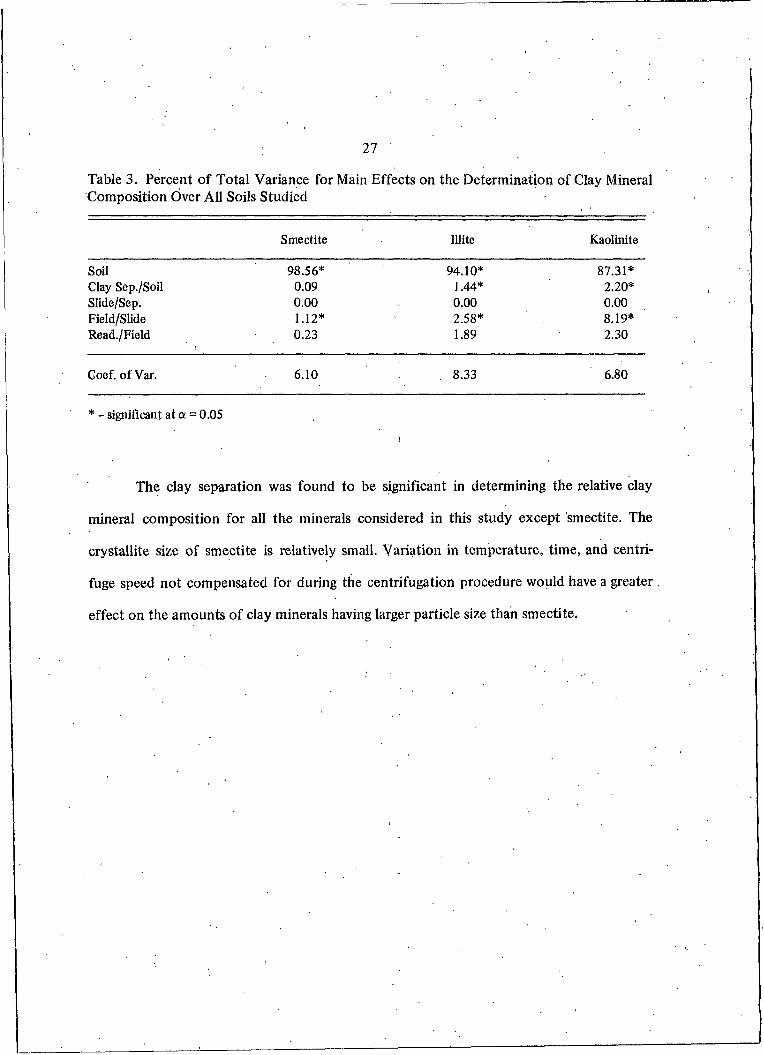
As may be seen in Table 3, the soil was found to be a significant source of variation.

Soil was the major source of variation for smectite, illite, and kaolinite. This was antici-. . I . •pated since the soils were chosen on their apparent clay mineral.composition.

The positioning of. the slide was also found to have a significant effect in deter

mining the relative clay mineral composition for each of the minerals tested.

27

Table 3. Percent of Total Variance for Main Effects on the Determination of Clay Mineral Composition Over All Soils Studied

Smectite Illite Kaolinite

Soil 98.56* 94.10* 87.31*Clay Sep./Soil 0.09 1.44* 2.20*Slide/Sep. 0.00 0.00 0.00Field/Slide 1.12* 2.58* 8.19*Read./Field 0.23 1.89 2.30

Coef. of Var. 6.10 . 8.33 6.80

* - significant at a = 0.05

The clay separation was found to be significant in determining the relative clay

mineral composition for all the minerals considered in this study except smectite. The

crystallite size of smectite is relatively small. Variation in temperature, time, and centri

fuge speed not compensated for during the centrifugation procedure would have a greater

effect on the amounts of clay minerals having larger particle size than smectite.

28

II. MAIN STUDY-QUANTIFICATION

The accuracy and precision of each modification of the factor method tested in

this study were determined by linear regression analysis. In this way measured parameters,

were compared with related estimated parameters. Complete peak area measurements ap

pear in Table 31.

Cation Exchange Capacity Estimation

. Linear regression models were developed to determine the relationship of the

cation exchange capacity of the clay-sized fraction as estimated from X-ray diffraction

results (ECEC) to the CEC of the same clay fraction as determined by chemical methods

(MCEC) for each of the modifications tested. Regression models of MCEC as estiinated

from levels of ECEC also permit an assessment of the variability of MCEC for any level

of ECEC. Table 4 contains the linear models and associated statistics developed for the ten

modifications tested in this study.

Table 4. Linear Regression Models of the Measured CEC on Estimated CEC

Slope Intercept r F SEE

Mod. I 0.683 3.66 0.927* 0.859 6.52Mod. II 0.684 4.43 0.936* 0.877 6.10Mod. Ill .0.688 4.97 0.939* ■ 0.881 6.01Mod. IV 0.697 . 5.50 0.941* 0.886 5.87Mod. V 0.750 7.11 0.949* 0.900 5.51.Mod. VI 0.733 3.01 0:932* 0.869 6.29Mod. VII 0.739 3.82 0.935* 0.875 6.15Mod. VIII 0.741 ‘ . 4.43 0.937* 0.878 6.07Mod. IX 0.750 5.02 0.940* 0.883 5.94Mod. X 0.815 6.64 0.946* 0.895 5.63


29

Based on the interdependence between MCEC and ECEC as measured by the cor

relation coefficient (r), the coefficient of determination (r2), and the dispersion of MCEC

about the regression line as measured by the standard error of the estimate (SEE), Modi

fications IV, V, IX, and X were chosen as the best modifications tested. Complete data

tables for these, four modifications appear in Tables 32-35.

It may be assumed that if a modification accurately accounted for the CEC as

measured by chemical methods, the regression model developed would be of the form

MCEC = ECEC, where the regression line passes through the origin and has a slope of 1.0.

The modification providing a linear relationship with a slope and y-intercept closest to

these values may be assumed to provide the most accurate assessment of the suite of clay

minerals present in the clay-sized fraction.

Statistical results for these four modifications appear in Table 5. Confidence limits

have been applied for consideration of both the inherent accuracy and precision of these

modifications.

Table 5. Selected Linear Regression Models of Measured CEC on Estimated CEC

Mod. No. Slope Intercept r r2 SEE

IV 0.697 ±0.072 5.50+1.66 . 0.94* 0.89 . 5.87V 0.750+0.068 7.11 ±1.56 0.95* 0.90 5.51

IX 0.750+0.073 5.02 ±1.68 . 0.94* 0.85 5.94X 0.815+0.069 6.64 ±1.59 . 0.95* 0.90 5.63

\


30

A value for the y-intercept greater than 0.0 is evidence of a failure of the modifi

cation to completely account for the CEC of the clay-sized fraction as measured by chemi

cal methods and/of the error inherent in the methods employed in obtaining values for

both MCEC and ECEC. Since the values of the y-intercepts do not significantly differ from

each other for the four models considered here it might be assumed that the error involved

in estimating CEC is constant for all of the modifications discussed. The positive intercepts

could be caused by one or more of several things. A few erroneously high measured CEC

values (MCEC) on samples dominated by low CEC clays would have this effect. Another

possible explanation is that the CEC of the clay minerals occurring in samples varied from

those assumed in estimating the CEC of the clay fraction. Alternatively, the positive inter

cepts may indicate the presence, of additional minor, low CEC constituents of the clay

sized fraction, such as feldspars.

Smectite, when present in a suite of clays, significantly affects both the estimated

and measured values of CEC. Overestimation of smectite would tend to reduce the slope

of these graphs to some value less than 1.0. A comparison of the slopes obtained for the

regression models of MCEC on ECEC for the four modifications discussed here reveals that

all of the modifications apparently overestimate smectite, since all of the slopes are signifi

cantly less than 1.0 (a = 0.05). Of these four modifications, Modification X has the liighest

value for the slope of the model, coupled with favorable values for the y-intercept, .r, r2.,

and SEE.

Graphical representation of this relationship for Modification X appears in Fig. 2.

The regression model given by MCEC = 0.815 (ECEC) + 6.64 approximates the expected

relationship given by ECEC = MCEC represented by the dashed line. The graphs are simul-

31

y = 0.815x + 6.64 r = 0.95

r2 = 0.90 SEE = 5.63

10 20 30 40 50 60 70 80Estimated CEC (meq/100 g clay)

Figure 2. Linear Regression Model of Measured CEC on Estimated CEC for Modification X.

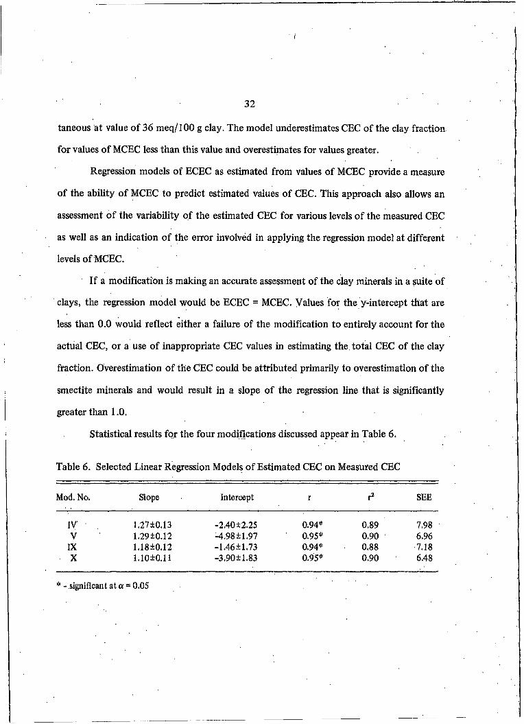
32

• I

taneous at value of 36 meq/100 g clay. The model underestimates CEC of the clay fraction

for values of MCEC less than this value and overestimates for values greater.

Regression models of ECEC as estimated from values of MCEC provide a measure

of the ability of MCEC to predict estimated values of CEC. This approach also allows an

assessment of the variability of the estimated CEC for various levels of the measured CEC

as well as an indication of the error involved in applying the regression model at different

levels of MCEC.

If a modification is making an accurate assessment of the clay minerals in a suite of

clays, the regression model would be ECEC = MCEC. Values for the y-intercept that are

less than 0.0 would reflect either a failure of the modification to entirely account for the

actual CEC, or a use of inappropriate CEC values in estimating the. total CEC of the clay

fraction. Overestimation of the CEC could be attributed primarily to overestimation of the

smectite minerals and would result in a slope of the regression line that is significantly

greater than 1.0.

Statistical results for the four modifications discussed appear in Table 6.

Table 6. Selected Linear Regression Models of Estimated CEC on Measured CEC


IV 1.27±0.13 -2.40±2.25 0.94* 0.89 7.98V 1.29±0.12 -4.98+1.97 0.95* 0.90 6.96

IX 1.18±0.12 -1.46+1.73 0.94* 0.88 7.18X 1.10±0.11 -3.90±1.83 0.95* 0.90 6.48


33

If, for any one value of CEC for the clay fraction one and only one suite of clay

minerals exists, it might be assumed that the SEE for the regression models of MCEC on

ECEC would equal the SEE for the regression models of ECEC on MCEC. Values of SEE

for the regression models of ECEC on MCEC3 for all the modifications discussed, are higher

than those reported for the regression models of MCEC on ECEC, The variability of ECEC

for any level of MCEC is greater than the variability of MCEC for any value of ECEC. This

is because the clay mineral estimates exhibit greater variability than do values for measured

CEC. This indicates that, in practice, due to the variability in X-ray diffraction results, one

measured value of CEC does not represent a unique suite of clay minerals. As in the case

of the regression models of MCEC on ECEC, the mean value for the slopes and intercepts

indicate that these modifications tend to underestimate the CEC at lower levels of MCEC

and overestimate the CEC when significant amounts of smectite are present.

If any of the values for the CEC of each mineral group varies significantly from the

actual Value it would be reflected in a slope different than 1.0. The slope obtained for the

regression model testing Modification X does not significantly (a = 0.05) differ from 1.0.

The value for the y-intercept does significantly differ from 0.0. Since the y-intercepts

of the models discussed do not significantly differ from each other, the difference between

the y-intercepts of the expected model and the model actually obtained is probably due

either to erroneously high measured CEC values or to the presence of a mineral group that

was not considered in estimating the composition of the clay-sized fraction. This parallels

the results of the regression models developed for MCEC on ECEC.

From Fig. 3 it may be seen that the regression model of Modification X for ECEC

on MCEC given by ECEC = 1.10(MCEC) - 3.90, closely follows the expected relationship

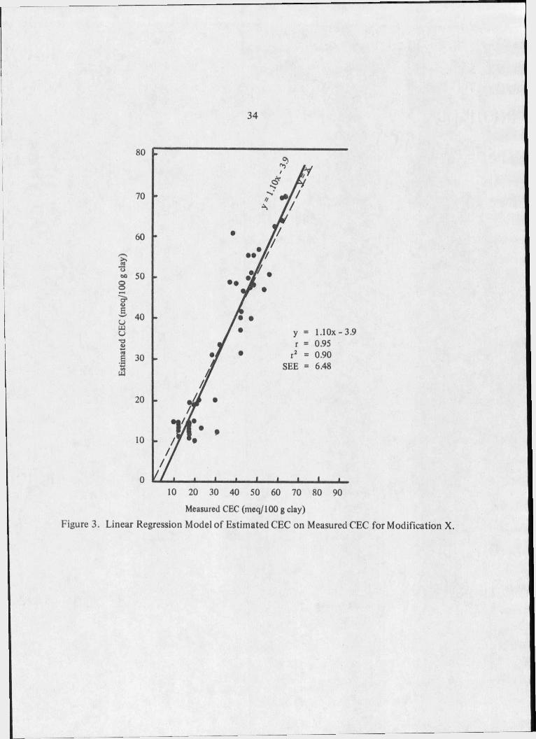
34

I.IOx - 3.9

10 20 30 40 50 60 70 80 90Measured CEC (meq/100 g clay)

Figure 3. Linear Regression Model of Estimated CEC on Measured CEC for Modification X.

35

given by ECEC = MCEC represented by the dashed line. The graphs are seen to be simul

taneous at a value of 39 meq/100 g. The model underestimates the CEC for values of

MCEC less than this value and overestimates for values of MCEC greater than 39 meq/

100 g. The percent error may be calculated by the following:

where, y = I .IO(MCEC) - 3.90 = the predicted ECEC

and y = MCEC = the expected value of ECEC assuming ECEC = MCEC

y - ythen %-error = ------ X 100, and the sign indicates underestimation (-)

y or overestimation (+).

From these calculations it was found that in the portion of the regression model

corresponding to values of MCEC less than 20 meq/100 g the error is greater than 11%. It

should be remembered, however, that in this portion of the graph the values of both MCEC

and ECEC are themselves small and relatively small errors in terms of meq/100 g cor

respond to large errors when expressed as percent. At these low levels of CEC, illite and

kaolinite typically dominate the exchange complex. Consequently, small differences in the

ECEC could be the product of significant errors in estimating the amounts of these

minerals.

The percent error involved in estimating CEC from this regression model in the area

of the graph corresponding to values of MCEC greater than 30 meq/100 g is less than 5%.

Consequently, Modification X appears to be most sensitive in determining the clay mineral

composition for those clay-sized fractions containing significant amounts of smectite.

Further, Modification X provides the greatest range in values over which it acceptably esti

mates clay mineral composition of the clay fraction.

36

Smectite Estimation

A more usable relationship is that of the estimated percent smectite composition

(ESM) as determined by the measured CEC. These regression models present a direct pre

dictive tool for the determination of smectite based on the measured CEC of the clay

sized fraction and permit a measure of the precision of the estimate (SEE).

Statistical results and confidence limits (a = 0.05) for the slope and y-intercept

appear in Table 7.

Table 7. Selected Linear Regression Models of Estimated Smectite Content on Measured Cation Exchange Capacity

Mod. No. Slope Intercept r T2 SEE

IV 1.49+0.13*1.22+0.13

-21.7812.27 0.96** 0.91 8.03

V 1.35+0.11 *1.21 ±0.11

-20.7811.94 0.96** 0.92 6.87

IX 1.37+0.12*1.21+0.12

-20.5912.10 0.96** 0.91 7.42

X 1.23±0.10*1.19+0.10

-19.41 + 1.78 0.96** 0.92 6.30

* - slopes of the expected regression model derived by substituting 100meq/l OOg at 100% smectite content ** - significant at a = 0.05

Expected models were derived from the regression models developed for each

modification assuming a MCEC of 100 meq/100 g at 100% smectite. This expected model

appears as a dashed line in Fig. 4 along with the graphical representation of the confidence

interval for the regression model obtained (dotted line).

;

37

. •• //

1.23x-19.41i = 0.96

10 20 30 40 50 60 70 80 90 100Measured CEC (meq/100 g clay)

Figure 4. Linear Regression Model of Estimated Smectite Content on Measured Cation Exchange Capacity.

38

The y-intercepts obtained for these relationships did not significantly differ from

each other and are related to the x-intercepts which correspond to the average CEC of the

clay-sized fraction when no smectite is present. As may be seen from Table 7 the slopes of

the expected regression models do not significantly differ. Consequently, the expected

models are similar for all of the modifications tested.

Expected models were derived from the regression models developed for each

modification assuming a MCEC of 100 meq/100 g at 100% smectite. This expected

model appears as a dashed Ifne in Fig. 4 along with the graphical representation of the

confidence interval for the regression model obtained (dotted line).

The y-intercepts obtained for these relationships did not significantly differ from

each other and are related to the x-intercepts which correspond to the average CEC of the

clay-sized fraction when no smectite is present. As may be seen from Table 7 the slopes of

the expected regression models do not significantly differ. Consequently, the expected

models are similar for all of the modifications tested.

Overestimatioh of the percent smectite composition would tend to increase the

slopes of these relationships. Assuming that the values for the y-intercepts relate to a con

stant and true average of the CEC of the clay-sized fraction when no smectite is present,

the preferable modification would be indicated by a regression model that closely esti

mated the expected regression model and did not significantly differ from it. It may be

seen from Fig. 4 that this is true of the regression model developed for Modification X.

The graph of the expected and derived regression models are nearly concurrent and the

expected model lies well within the 95% confidence interval applied to the derived regres

sion model for this modification. The coefficient of determination indicates that approxi

39

mately 92% of the variation in the percent smectite composition was explained by vari

ations in the measured CEC.

The error involved between the expected and the derived models was approxi

mately 3% at MCEC =100 meq/100 g clay. Less than 3% error is incurred in estimating

the relative smectite content at lower values of measured CEC.

A limiting factor in applying this relationship to the prediction of levels of smec

tite content is the apparent low level of precision as indicated by an SEE = 6.30. The 95%

confidence interval for any value of the percent smectite in a sample predicted from the

measured CEC of the clay-sized fraction would be approximately ± 12.6 percent smectite.

The difference between the measured CEC (MCEC) subtracted from the estimated

CEC (ECEC) was used as a dependent variable (ECDIF) in testing relationships with ESM

to assess any effect the apparent relative smectite composition might have on estimating

accuracy. In the above discussions it was shown that accuracy is generally lower for esti

mates of the smectite content in samples containing low amounts of smectite when the

error is expressed on a percentage basis. The regression models developed for ECDIF on

ESM provide a direct indication of bias and an avenue for determining the significance of

the apparent bias.

Statistical results for the four best modifications tested appear in Table 8. Confi

dence limits have been applied to the slope and y-intercept to facilitate the assessment of

the significance of the apparent bias implied by the slope and intercept of the model.

Modifications providing accurate and unbiased estimates of the suite of clay min

erals should reveal a relationship that is concurrent with the x-axis and is of the form

ECDIF = 0, with r = 0, r2 = 0, and SEE = 0.0. Regression models testing the modifications

40

Table 8. Selected Linear Regression Models of the Difference in Estimated and Measured Cation Exchange Capacity on Estimated Smectite Content

Mod. No. Slope Intercept .. r r2 SEE

IV 0.248+0.067 -0.32±1.77 0.73* 0.53 6.28V 0.217 ±0.067 -3.81 ±1.62 0.68* 0.46 5.72

IX 0.198 ±0.073 -0.63 ±1.79 0.62* 0.38 6.33X 0.151 ±0.076 -3.83 ±1.66 0.50* 0.25 5.86

* - significant a t« = 0.05

that significantly differ from this perfect fit relationship indicate significant bias in making

estimates of the clay mineral composition. Ovefestimation of the amount of smectite

would tend to increase the slopes of these models and decrease the value of the y-intercept.

Of primary importance in analyzing these relationships is the slope and y-intercept

of the regression models obtained. From Table 8 it may be seen that the slopes of all the

regression models significantly differ from 0.0. Consequently, it may be assumed that bias

is incurred in estimating the clay mineral composition by any of the four modifications dis

cussed. However, the results indicate that Modification X provides the most accurate and

relatively unbiased assessment of the clay mineral composition. Modification X has the

lowest slope; Modifications IV and IX do include 0.0 in the 95% confidence interval. The

y-intercept for Modification X is reasonably close to zero. In addition the r, r2, and SEE

values for Modification X are lowest of the modifications discussed.

These results tend to support those previously reported for the regression models

developed for ECEC on MCEC, MCEC on ECEC and ESM on MCEC. From Fig. 5 it is

observed that the graphs of the expected and derived models are simultaneous at a value

41

y = 0.151x-3.83 r = 0.499

I2 = 0.249 SEE = 5.86

10 20 30 40 50 60 70 80Estimated Smectite Content (%)

Figure 5. Linear Regression Model of the Difference in Estimated and Measured Cation Exchange Capacity on Estimated Smectite Content.

42

of approximately 25 percent smectite. The regression model indicates that Modification

X tends to overestimate the amount of smectite present when it is greater than this amount

and underestimate the amount o f smectite when it is less than this amount. Modification X

also tends to favor lower estimated amounts of illite. In the portion of the graph represent

ing low smectite composition the suite of clay minerals would be dominated by illite and

kaolinite. Consequently, Modification X should be expected to yield lower estimates of the

CEC in samples dominated by illite.

Illite Estimation

As a further test of the accuracy of the mineral estimates, regression models were

developed to examine the relationship of the relative composition of illite (EIL) in each

sample with the percent illite based on total K analysis assuming 8.3% (MILS) and 5.1%

(MILS) elemental K per unit cell of illite. Regression models of EIL as estimated from

values of MILS and MILS provide a measure of the sensitivity of the chemical methods

employed to account for variation in apparent percent composition of illite in the clay

sized fraction. They also allow an assessment of the variability of the estimated percent

illite for various levels of MILS and MILS as well as the error involved in applying the

regression model at various levels on MILS and MILS.

It may be assumed that if a modification accurately estimated the percent illite

and all of the K. present in the clay-sized fraction was a component of the crystalline

structure of illite then the expected regression model developed would be PIL = MILS

or MILS. This regression line would pass through the origin and have a slope of 1.0. The

modification providing a linear relationship with a slope and y-intercept closest to these

43

values may be assumed to provide the most accurate assessment of the relative amount of

illite present in the clay-sized fraction. Values for the y-intercept that are less than 0.0

would reflect a failure of the modification to entirely account for the relative amount of

illite as estimated by total K analysis.

Models derived assuming 8.3% elemental K per unit cell illite. Statistical results for

the four best modifications appear in Table 9. Confidence limits (a = 0.05) have been ap

plied for consideration of both the accuracy and the precision of these modifications.

Table 9. Selected Linear Regression Models of Estimated Illite Content on Measured Illite Content (Assuming 8.3% K per Unit Cell Illite)

Mod. No. Slope Intercept r r$ SEE

IV 1.63 ±0.24 -11.12±1.73 0.87* 0.75 6.10V 1.03 ±0.15 -4.83±1.10 0.87* 0.75 3.90

IX 1.58±0.23 -9.22±1.67 . 0.87* 0.76 5.92X 0.99 ±0.15 -3.31 ±1.09 0.86* 0.74 3.87


The y-intercepts of all the regression models (Table 9) are significantly less than

0.0. These negative intercepts support the conclusions made from the regression models

developed for ECEC on MCEC, particularly that the inability of the modifications to com

pletely explain the percent illite derived from total K analysis is due to the presence of a

K-bearing mineral in the clay-sized fraction that caused an overestimation of the relative

amount of illite. It may be seen, however, that there is a significant difference between the

y-intercepts obtained for these models. While the y-intercepts of the regression models for

Modifications IV and IX do pot significantly differ from each other, they do significantly

44

differ from the intercepts obtained for the models testing Modifications V and X. The

latter modifications do not significantly differ from each other. It should be noted that

Modifications IV and IX tend to cause higher estimates of smectite and illite while Modi

fications V and X tend to favor higher estimates of kaolinite at the expense of the esti

mated smectite and illite contents.

If the modification is sensitive to the changes in illite content as determined by

total potassium analysis and the K-content of the illite is 8.3%, the slope of the regres

sion model testing that modification should not significantly differ from 1.0. In Figs. 6

and 7 it may be seen that the regression models closely parallel the expected models and

differ in both cases by a relatively constant amount.

The constancy of the difference between the expected and derived regression

model might also indicate the use of an inappropriate combination of coefficients in

the characterization of the peak areas. As stated earlier it might be reasonable to expect

such a relationship if the procedure used to estimate the mineral components of the clay

sized fraction failed to recognize a K-bearing mineral of minor, relatively constant,

proportions.

Values for SEE indicate lower variability for EIL at any given level of MILS for

Modifications V and X. SEE values were much higher for the regression models testing

Modifications IV and IX.

Modification X seems to provide the most favorable combination of accuracy and

precision for the estimation of illite of the four modifications discussed here. The regres

sion model testing this modification is given by EIL = 0.99 (MILS) - 3.31. This closely folr

lows the expected relationship given by EIL = MILSi The coefficient of determination

45

10 20 30 40 50 60Measured Fllite Content (%)

Figure 6. Linear Regession Model of Estimated Illite Content on Measured Illite Content (8.3% K) for Modification V.

46

0.99x-3.31

Measured Dlite Content (%)

Figure 7. Linear Regression Model of Estimated Illite Content on Measured Illite Content (8.3% K) for Modification X.

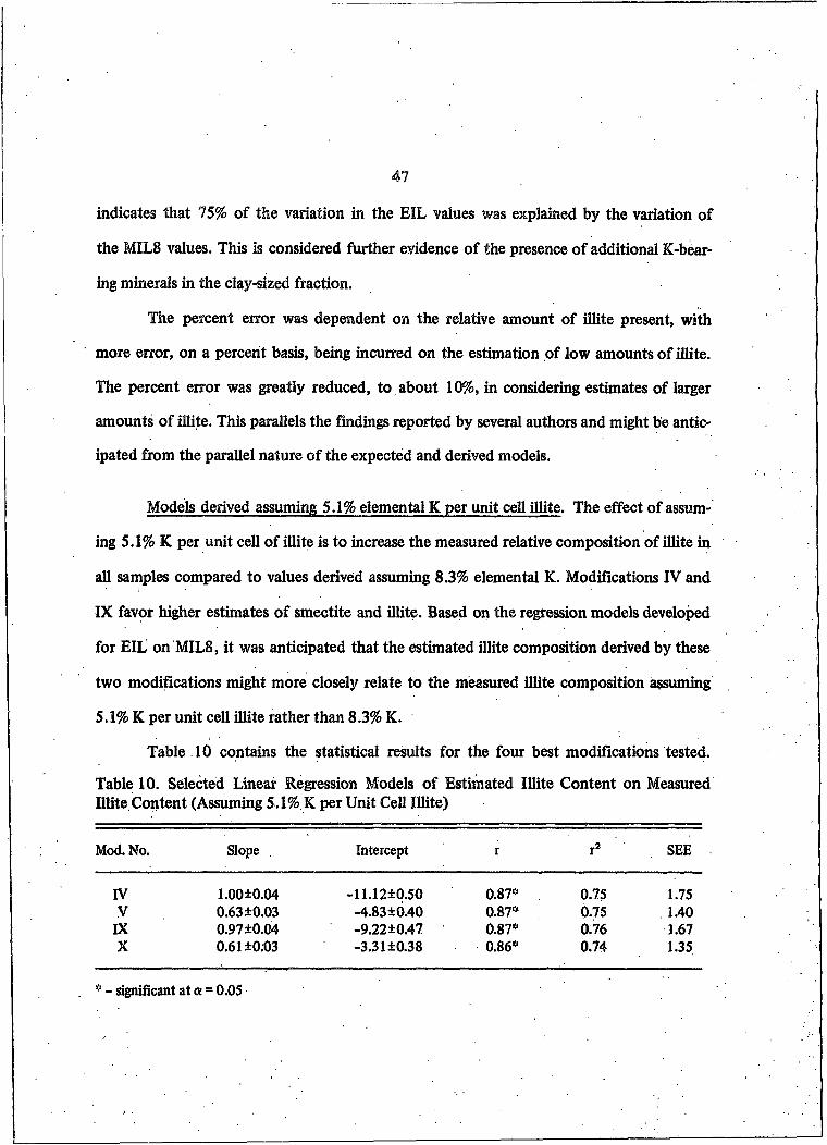
47

indicates that 75% of the variation in the EIL values was explained by the variation of

the MILS values. This is considered further evidence of the presence of additional K-bear-

ing minerals in the clay-sized fraction.

The percent error was dependent on the relative amount of illite present, with

more error, on a percent basis, being incurred on the estimation of low amounts of illite.

The percent error was greatly reduced, to about 10%, in considering estimates of larger

amounts of illite. This parallels the findings reported by several authors and might be antic

ipated from the parallel nature of the expected and derived models.

Models derived assuming 5.1% elemental K per unit cell illite. The effect of assum

ing 5.1% K per unit cell of illite is to increase the measured relative composition of illite in

all samples compared to values derived assuming 8.3% elemental K. Modifications IV and

IX favor higher estimates of smectite and illite. Based on the regression models developed

for EIL on MILS, it was anticipated that the estimated illite composition derived by these

two modifications might more closely relate to the measured illite composition assuming

5.1% K per unit cell illite rather than 8.3% K.

Table 10 contains the statistical results for the four best modifications tested.

Table 10. Selected Linear Regression Models of Estimated Illite Content on Measured Illite Content (Assuming 5.1% K per Unit Cell Illite)

Mod. No. Slope Intercept r I 2 SEE

IV 1.00±0.04 -11.12±0.50 0.87«" . 0.75 1.75V 0.63 ±0.03 -4.83±0.40 0.87* 0.75 1.40

IX 0.97 ±0.04 -9.22±0.47 0.87* 0.76 1.67X 0.61 ±0.03 -3.31 ±0.38 0.86* 0.74 1.35


48

The slopes of the regression models testing Modifications IV and IX do not differ

from the perfect fit slope of 1.0. However, these modifications more seriously underesti

mated relative Eite content in comparison with measured values assuming 5.1% K per unit

cell illite than did Modifications V and X in similar comparisons assuming 8.3% K. These

results indicate that for the samples used in this study the 8.3% value is a more accurate

measure for the relative K-content per unit cell E ite than is 5.1%. Consequently, the dis

cussion and conclusions drawn based on the models of EIL derived from MILS appear to

be more appropriate.

To assess the bias in estimating the relative Eite composition that is related to the

estimated percent composition of Eite, the difference between MILS subtracted from EIL

was used as a dependent variable (ILDIF8) in developing regression models with EIL. Sta

tistical results for the four best modifications tested appear in Table 11.

Table 11. Selected Linear Regression Models of the Difference in Estimated and Measured Illite Contents on Estimated Illite Content (Assuming 5;1% K per Unit Cell IEte)

Mod. No. Slope Intercept i r2 SEE

IV 0.519 ±0.075 -10.30±0.98 0.89* 0.80 3.48V 0.237 ±0.116 -8.61 ±0.97 0.51* 0.26 3.43

IX 0.501 ±0.077 -9.46 ±0.98 0.88* 0.78 3.45X 0.219±0.124 -7.83 ±1.00 0.45* 0.45 3.54


Modifications providing accurate and unbiased estimates of the suite of clay min

erals should reveal a relationsEp that is concurrent with the x-axis and is of the form

ILDIF8 = 0, with r = 0, r2 = 0 , and SEE = 0. Underestimation of the relative amount of

illite present would tend to decrease the value of the y-intercept. A positive slope for the

regression line indicates that the modification provides biased estimates of the percent

illite composition such that, above some point at which the derived and expected models

are simultaneous, the amount of overestimation is directly proportional to an increase in

the apparent relative composition of illite. Conversely, the amount of underestimation is

directly prdportipnal to a decrease in the percent illite composition. In addition, statisti

cally significant values for the r and r2 further indicate that the bias inherent in the modi

fication is significant.

From Table 11 it may be seen that the slope and correlation coefficients of all

the regression models discussed significantly differ from 0.0. It follows that bias is incur

red in estimating the relative composition of illite by any of the modifications discussed

here. It may be anticipated, from the results of the regression models developed for EIL

on MILS (Table 9) that the y-intercepts will significantly differ from 0.0. This was found

to be the case for all four modifications discussed.

Modifications X and V combine the lowest slope with a value for the y-intercept

that is in line with the results obtained for EIL on MILS. The r and r2 values are the lowest

of the modifications discussed. The SEE is slightly higher for Modification X, but it is not

felt that this indicates a significant increase in variabUity of the estimates compared to the

other modifications.

The regression model as shown in Fig. 8 indicates that Modification X underesti

mates the relative amount of illite present below a value of 35.8% illite (EIL). This cor

responds to the upper range of the percent illite composition as estimated by Modification

X. Consistent apparent underestimation of EIL coupled with a low, yet significant cor-

49

50

0.219x - 7.83r = 0.454

T2 = 0.206 SEE = 3.54

Estimated Illite Content (%)

Figure 8. Linear Regression Model of the Difference in Estimated and Measured Illite Content on Estimated Illite Content (assuming 8.3% K per unit cell I Hite).

51

relation coefficient, is interpreted to indicate a consistent overestimation of MILS. This

could be due to the presence of. an additional, but unmeasured, K-bearing mineral that

composes a small, relatively constant portion of the clay-sized fraction. However, a defi

nite conclusion based on the results of this study concerning the apparent underestimation

of illite is not possible. When the results of these regression models are considered in con

junction with the results previously reported here, it is felt that they indicate Modification

X is more responsive to the amount of illite in a sample.

Kaolinite Estimation

Measurements of the kaolinite content such as those made for illite content were

not made during this study. As a result the accuracy and precision of a modification’s

ability to estimate the relative composition of kaolinite was inferred from linear regression

models of the estimated kaolinite content (EKA) on the measured CEC (MCEC). Statistical

results and confidence limits (oz = 0.05) for the slope and intercept appear in Table 12 for

the four best modifications tested.

Table 12. Selected Linear Regression Models of Estimated Kaolinite Content on Measured Cation Exchange Capacity

Mod. No. Slope Intercept r r? SEE

IV -1.05 ±0.17 68.45 ±2.87 -0.88* q.77 . 9.98V -1.22±0.16 87.39±2.77 -0.91* 0.83 9.79

IX -1.02±0.16 . 68.36 ±2.74 -0.88* 0.77 9.70X -1.17±0.16 86.96±2,68 -0.91* 0.82 9.49


52

In general, samples exhibiting low values for measured CEC will possess high kaoli-

nite contents and low smectite content. The reverse is assumed to be true at high values for

measured CEC. As a result the slopes of the regression models of EKA oh MCEC should be

negative. As may be seen in Table 12 the slopes of the regression models testing the four

modifications discussed exhibit this negative relationship.

Kaolinite typically exhibits a relatively small CEC. In the presence of measureable

amounts of smectite, kaolinite is expected to compose a relatively small portion of the

total CEC of the clay-sized fraction. Further, it is assumed that relatively large Variations in

the estimated kaolinite content would not affect the CEC of the clay fraction as much as

a similar variation in smectite content. Consequently, it could be anticipated that theI

accuracy and precision of the modifications as measured by the regression models of EKA

on MCEC would be lower than that indicated by similar models developed for smectite

composition. The high values for the SEE obtained for all the modifications tested indicate

that these modifications estimate kaolinite content with less precision than either smectite

or illite. Modification X exhibited the lowest SEE (9.49).

The four modifications discussed exhibit significant correlation between the esti

mated kaolinite content and the measured CEC. The values of the intercepts and their

confidence intervals indicate that all four modifications significantly underestimate kaoli

nite at 100% kaolinite content. Modifications V and X tend to favor higher estimates for

kaolinite. These two modifications significantly differed from Modifications IV and IX but

not from each other. Since regression models testing the estimation of smectite and illite

content indicated that Modification X provided the best estimates of these minerals it

was assumed that this modification provided adequate estimation of kaolinite content as

53

well. The regression model for Modification X is given by EKA = -1.17 (MCEC) + 86.96,

with r = -0.91, r2 = 0.82, and SEE = 9.49. This relation is graphically presented in Fig. 9.

Linear regression models of ECDIF as related to EKA were developed to assess the

effect of the relative kaolinite composition has on the estimating accuracy. They appear in

Table 13.

Table 13. Selected Linear Regression Models of the Difference in Estimated and Measured Cation Exchange Capacity on Estimated Kaolinite Content


IV -0.318±0.1p6 17.28±1.81 -0.72* 0.52 8.69V -0.223 ±0.096 12.09±1.63 -0.67* 0.50 7.20

IX -0.238±0.106 . . 12.55±1.82 -0.60* 0.36 7.31X -0.150±0.096 6.64±1.66 -0.50* 0.25 6.03


The expected regression model is concurrent with the x-axis and is of the form

ECDIF = 0, with r = 0, r2 = 0, and SEE = 0. A significant difference between this perfect

fit model and the derived model indiates a significant bias in making estimates of the kaoli

nite content. Underestimation of the kaolinite content would tend to steepen the slopes of

the regression models and mcrease the value of the y-intercept. Data in Table 13 show that

. the slopes and y-intercepts significantly differ from 0.0. The correlation coefficients indi

cate relationships significant at a = 0.05. It may be assumed that bias is incurred in estimat

ing the relatively kaolinite content. The results indicate that Modification X provides the

most accurate and relatively unbiased assessment of the kaolinite composition. It combines

54

-1.17x +86.96 -0.91

SEE = 9.49

10 20 30 40 50 60 70 80 90 100Measured CEC (meq/100 g clay)

Figure 9. Linear Regression Model of Estimated Kaolinite Content on Measured Cation Exchange Capacity.

55

the lowest slope and y-intercept with the lowest value of r, r2, and SEE for any of the

modifications discussed.

These results seem to corroborate those previously reported for estimates of smec

tite and illite composition. The graphs of the expected and derived models for Modifi

cation X (Fig. 10) are simultaneous at a value of approximately 44% kaplinite. This indi

cates that Modification X underestimates CEC of the clay fraction at kaolinite contents

higher than 44% and overestimates CEC at kaolinite contents lower than this value. This

could result from an underestimation of kaolinite and/or an overestimation of smectite.

Previously it was shown that Modification X overestimates CEC and smectite at values of

smectite composition greater than 25 percent. The results indicate that Modification X

tends to underestimate kaolinite and overestimate smectite at values of relative kaolinite

and smectite composition greater than 44% and 25%, respectively. An apparent overesti

mation of kaolinite and underestimation of smectite occurs at compositions below these

values. Since regression models testing the accuracy of the illite estimations indicated a

consistent error not directly involved with the X-ray diffraction pattern characterization• .-

process, it is inferred that Modification X overestimates smectite and underestimates

kaolinite. These results indicate that further accuracy might be obtained by trying other

modifications of the factor method that reduce the characterized peak area of the 17A

peak while it increases the characterized peak area of the 7A peak.

56

y = -0.150x + 6.64 r = -0.50

T2 = 0.25 SEE = 6.03

— e.

10 20 30 40 50 60 70 80 90Estimated Kaolinite Content (%)

Figure 10. Linear Regression Model of the Difference in Estimated and Measured Cation Exchange Capacity on Estimated Kaolinite Content.

SUMMARY AND CONCLUSIONS

An assessment of the major sources of error in the X-ray diffraction procedure

was conducted in a preliminary study using a one-way analysis of variance for a nested

design for peak area and percent mineral composition. When considered over all soils

tested, the X-ray diffraction method used was found to be sensitive to the variations in

the mineralogy of the clay fraction of the soils used when considering peak area and rela

tive mineral composition. The positioning of the slide was found to be significant in

determining peak area and relative composition for all soils tested. Clay separation and

between slide effects were found to be significant sources of variation in specific instances

and seem to be particularly important in considering kaolinite content and those peaks

associated with kaolinite determination. The results indicate the need for extreme care and

consistency during all phases of sample preparation and presentation.

In the main study the accuracy of ten modifications of the factor method was

investigated. The results indicate that the factor method may be applied in X-ray diffrac

tion analysis to yield a relatively fast and reasonably accurate assessment of the dominant

clay minerals composing the clay fraction of arid and semi-arid land soils and their parent

material in southeastern Montana. The method seems particularly useful in making quanti-

tative estimations of smectite, illite, and kaolinite.

Linear regression models indicated that Modification X is most responsive to the

amount of smectite, illite and kaolinite in a sample. This modification yields accurate esti

mates for these clay minerals in material that does not contain significant amount of ver-

miculite and chlorite.

The following computations are used to calculate characterized peak areas for

Modification X:

58

17A Mg-sat. E.G./5 = Smectite Peak Area(14A Mg-sat. E.G. minus 14A K-sat. 350°C/2

= Vermiculite Peak Area14A K-sat. 350°C/2 = Chlorite Peak AreaIOA Mg-sat. E.G./1 . = Illite Peak Area(7A Mg-sat. E.G. minus 7A K-sat. 550°C)/4

= Kaolinite Peak Area(3.3A Mg-sat. E.G. minus 3/4 ( IOA Mg-sat. E.G.))/4

= Quartz Peak Area

Characterized peak areas are totaled and the relative percent composition of each mineral

calculated according to:

Smec. Pk. Area + Verm. Pk. Area + Chlor. Pk. Area + KaoL Pk. Area + Quar. Pk. Area = Total Peak Area

Percent Smectite = Smec. Pk. Area/Total Pk. Area X 100 Percent Vermiculite = Verm. Pk. Area/Total Pk. Area X 100 Percent Chlorite = Chlor. Pk. Area/Total Pk. Area X 100 Percent Illite = 111. Pk. Area/Total Pk. Area X 100 Percent Kaolinite = Kaol. Pk. Area/Total Pk. Area X 100 Percent Quartz = Quar. Pk. Area/Total Pk. Area X 100

Linear regression models involving CEC determined by chemical means (MCEC).

and the CEC estimated from X-ray diffraction analysis (ECEC) showed that 90% of the

variability of the predicted parameter could be accounted for by the measured parameter

using estimates derived by Modification X. The variability of ECEC for any level of MCEC

is greater than the variability of MCEC for any level of ECEC. This indicates that in prac-,

tice, due to the variability in the X-ray results, one measured value of CEC does not repre

sent a unique suite of clay minerals as determined by X-ray diffraction analysis.

Measurement of illite content by total K analysis was conducted assuming 8.3%

and 5.1% elemental K per unit cell illite. The results of linear regression analysis indicated

that measurements made using the 8.3% K value more accurately depicted the estimated

illite content.

Using estimates derived by Modification X predictive regression models for the esti

mation of the relative compositions of smectite, illite and kaolinite were developed based

on values of measured CEC and the percent composition of illite as determined by total K

analysis (MILS):

%-smectite (± 12.6%)= 1.23(MCEC) - 19.41, r2> 0.92

%-illite . (+; 7.7%)= 0.99(MILS)- 3.31, r2 =0.74

%-kaolinite(± 19.0%) = -1 .17(MCEC) + 86.96,r2 = 0.82 .

The relative amount of illite was frequently underestimated. The apparent under

estimation could be caused by variability in the K per unit cell of illite resulting in over

estimation of illite from total K analysis. This is supported by the moderate r2 value. Im

proper factors employed in characterizing peak areas might have been responsible for the

apparent underestimation, but, this is not supported by the slope of the regression. Alter

natively, the y-intercept of this model could indicate either a threshold amount of illite

that must be present to be recognized by the X-ray diffraction machine or could indicate

the presence of an additional, K-bearing, nonmicaceous mineral such as feldspar in small

constant amounts that was not considered in estimating the mineral composition of the

clay-sized fraction of the samples studied.

Modification X fended to overestimate smectite and underestimate kaolinite at

values of relative smectite and kaolinite composition greater than 25% and 44%, respec

tively. An apparent overestimation of kaolinite and underestimation of smectite occurs

at compositions below these values. Since regression models testing the accuracy of the

59

60

illite estimations indicated a consistent error not directly involved with the X-ray diffrac

tion pattern characterization process, it was inferred that Modification X overestimates

smectite and underestimates kaolinite.

Significant bias caused by the apparent amount of the mineral present was found

for all modifications tested in estimating smectite, illite and kaolinite. However, Modifi

cation X was shown to be least affected by the amount of mineral present. Based on a

comparison of the SEE and r2 values, the estimates of the relative illite composition ap

pear to be less accurate than estimates of the relative smectite content. Illite and smectite

are estimated with greater accuracy and precision than kaolinite.

LITERATURE CITED

LITERATURE CITED

I . Alexander, L. and H. P. King. 1948. Basic aspects of X-ray absorption in quantitative diffraction analysis of powder mixtures. Anal. Chem. 20:886-889.

2. Biscayne, P. E. 1965. Mineralogy and sedimentation of recent deep-sea clay in the ■ Atlantic Ocean and adjacent seas and oceans. Geol. Soc. Amer. Bull. 76:803-832.

3. Brindley, G. W.. 1961. Quantitative analysis of clay mixtures. /« G. Brown, ed. The X-ray Identification and Crystal Structures of Clay Minerals. Mineralogical Society^ London.

4. Brindley, G. W. and Hsein Ming Wan. 1974. Use of long-spacing alcohols and alkanes for calibration of long spacing from layer silicates particularly clay minerals. Clays and Clay Minerals 22:313-317.

5. Carrol, D. 1970. Clay Minerals: A guide to their X-ray identification. Special Paper 126, The Geological Society of America. Boulder, Colorado.

6. Cullity, B. D. 1956. Elements of X-ray Diffraction. Addison-Wesley Publishing Co., Inc., Reading, Massachusetts.

7. Day, P. R. 1965. Particle fractionation and particle-size analysis, pp. 545-567. In C. A. Black, ed. Methods of Soil Analysis, Part I. Agronomy No. 9. Amer. Soc. of Agron., Madison, Wisconsin.

8. Edwards, A. P. and J. M. Bremrier. 1964. Use of sonic vibration for separation of. soil particles. Can. J. of Soil Sci. 44:366.

9. Edwards, A. P. and J. M. Bremner. 1967. Dispersion of soil particles by sonic vibration. Jour. Soil Sci. 18:47-63.

10. Emerson, W. W. 1971. Determination of the contents.of clay-sized particles in soils. Jour. Soil Sci. 22:50-59.

11. Freas, D. H. 1962. Occurrence, mineralogy and origin of the, lower Golden Valley kaolinite clay deposits near Dickinson, North Dakota. Bull. Geol. Soc. Amer. 73: 1341-1363.

12. Genrich, D. A. and J. M. Bremner. 1972. A reevaluation of the ultrasonic-vibration . method of dispersing soils. Soil Sci. Soc. Amer. Proc. 36:944-947.

63

13. Gibbs, R. J. 1965. Error due to segregation in quantitative clay mineral X-ray diffraction mounting techniques. Am. Mineral. 50:741-751.

14. Gibbs, R. I. 1967. Quantitative diffraction analysis using clay mineral standards extracted from the samples to be analyzed. Clay Minerals 7:79-90.

15. Glenn, G. R. and R. L. Handy. 1961. Quantitative determination of soil mohtmoril- lonite by X-ray diffraction. Am. Soc. Testing and Materials Proc. 61:1277-1289.

16. Harward, M. E. and A. A. Thiesen. 1962. Problems in clay mineral identification by X-ray diffraction. Soil Sci. Soc. Amer. Proc. 26:336-341.

17. Harward, M. E., A. A. Thiesen, and D. D. Evans. 1962. Effect of iron-removal and dispersion methods on clay mineral identification by X-ray diffraction. Soil Sci. Soc. Amer. Proc. 26:535-541.

18. Jackson, M. L. 1956. Soil Chemical Analysis—Advanced Course. Published by author. University of Wisconsin, College of Agriculture, Dept, of Soils, Madison, Wisconsin.

19. Jarvis, N. L., R. D. Dragsdorf, and R. Ellis, Jr. 1957. Quantitative determination of clay mineral mixtures by X-ray diffraction. Soil Sci. Soc. Amer. Proc. 21:257-260.

20. Johns, W. D., R. E. Grim, and W. R. Bradley. 1954. Quantitative estimations of clay minerals by diffraction methods. Jour, of Sed. Petrol. 24:242-251.

21. Keller, G. H. and A. F. Richards. 1967. Sediments of the Malacca Strait, Southeast Asia. Jour, of Sed. Petrol. 37:102-127.

22. Kinter, E. B. and S. Diamond. 1956. A new method for preparation and treatment of oriented aggregate specimens of soil clays for X-ray diffraction analysis. Soil Sci. 81:111-120.

23. Kittrick, J. A. and E. V. Hope. 1963. A procedure for the particle-size separation of soils for X-ray diffraction analysis. Soil Sci. 96:319-325.

24. Klug, H. P. 1953. Quantitative analysis of powder mixtures with the Geiger-counter spectrometer. Anal. Chem. 25:704-708.

25. Klug, H. P., L. Alexander, and E. Kimmer. 1948. Quantitative analysis with the X-ray spectrometer—accuracy and reproducibility. Anal. Chem. 20:607-609.

64

26. Kunze, G. W. 1955. Anomalies in the ethylene glycol solvation techniques used in X-ray diffraction. Proc. of the 3rd Natl. Conf. on Clays and Clay Minerals 3:88-93..

27. Kunze, G. W. 1965. Pretreatment for mineralogical analysis, pp. 568-577. In C. A. Black, ed. Methods of Soil Analysis, Part I. Agronomy No. 9, Amer. Soc. of Agron., Inc., Madison, Wisconsin.

28. Leroux, J., D. H. Lennox, and K. Kay. 1953. Direct quantitative X-ray analysis by diffraction-absorption technique. Anal. Chem. 25:740-743.

29. Meade, R. H. 1967. Petrology of sediments underlying areas of land subsidences in Central California. U.S. Geological Survey Prof. Paper 497-C.

30. Mehra, 0 . P. and M. L. Jackson. 1959. Constancy of the sum of mica unit cell potassium surface and interlayer sorption surface in vermiculite-illite clays. Soil Sci. Soc. Amer. Proc. 23:101-105.

31. McNeal, B. L. 1966. Clay mineral variability in some Punjab soils. Soil Sci. 102:53-58.

32. McNeal, B. L. 1968. Limitations of quantitative soil clay mineralogy. Soil Sci. Soc. Amer. Proc. 32:119-121.

33. Moore, C. A. 1968. Quantitative analyses of naturally occurring multicomponent mineral systems by X-ray diffraction. Clays and Clay. Mineral. 16:325-326.

34. Neiheisel, J. and C. E. Weaver. 1967. Transport and deposition of clay minerals, Southeastern United States. Jour, of Sed. Petrol. 37 :1084-1116. .

35. Nie, N. H., C. H. Hull, J. G. Jenkins, K. Steinbrenner, and D. Brent. 1970. SSPS, Statistical Package for the Social Sciences, Second Edition. McGraw-Hill Book Company, Inc., New York, NY. b75pp.

36. Norrish, K. and R. M. Taylor. 1962. Quantitative analysis by X-ray diffraction. Clay. Minerals Bull. 5:98-109.

37. Olmstead, L. B. 1931. Dispersion of soils by a supersonic method. Jour. Agr. Res. 42:841-852.

38. Parrish, W. 1960. Advances in X-ray diffractdmetry of clay minerals. Proc. of the 7th Natl. Conf. on Clays and Clay Mineral. 7:230-259.

65

39. Pierce, J. W. and F. R. Siegel. 1964. Quantification in clay mineral studies of sediments and sedimentary rocks. Jour, of Sed. Petrol. 39:187-193.

40. Pratt, P. F. 1965. Potassium. In C. A. Black, ed. Methods of Soil Analysis, Part II. pp. 671-698. Amer. Soc. of Agron., Inc., Madison, Wisconsin.

41. Quakemaat, J. 1970. Direct diffractrometric quantitative analysis of synthetic clay mineral mixtures with MoS2 as orientation indicator. Jour. Sed. Petrol. 40:506-513.

42. Schoen, R. 1962. Semi-quantitative analysis of chlorites by X-ray diffraction. Amer. Mineral. 47:1384-1392.

43. Schoen, R., E. Foord, and D. Wagner. 1972. Quantitative analysis of clays. Problems, achievements, and outlook. Proc. of the Internat. Clay Confi 1972. Madrid, Spain. 787-796.

44. Schultz, L. G. 1955. Quantitative evaluation of the kaolinite and illite in underclays. Proc. of the 3rd Natl. Cohfi on Clays and Clay Mineral. 3:421-429.

45. Schultz, L. G. 1960. Quantitative X-ray determinations of some aluminous clay minerals in rocks. Proc. of the 7th Natl. Confi on Clays and Clay Mineral. 7:216-224.

46. Sokal, R. R. and F. J. Rohlf. 1969; Biometry. W. H. Freeman and Company, San Francisco, CA.

47. Talvenheimo, G. and J. L. White. 1952. Quantitative analysis of clay minerals with the X-ray spectrometer. Anal. Chem. 24:1784-1789.

48. Tanner, C. B. and M. L. Jackson. 1947. Nomographs of sedimentation times for soil particles under gravity or centrifugal acceleration. Soil Sci. Soc. Anier. Proc. 12:60-65.

49. Taylor, R. M. and K. Norrish. 1966. The measurement of orientation distribution and its application to quantitative X-ray diffraction analysis. Clay Mineral. 6:127-124.

50. Thiesen, A. A. and M. E. Harward. 1962. A paste method for preparation of slides for clay mineral identification by X-ray diffraction analysis. Soil Sci. Soc. Amer. Proc. 26:90-91.

51. To we, K. M. 1974. Quantitative clay petrology: The trees but not the forest? Clays and Clay Mineral. 22:375-378.

52. Vladimirov, V. Ye. 1968. Study of the effects of acoustic vibrations on the physio- chemical properties of a soil suspension. Soviet Soil Scii 5:654-659.

53. Watson, J. R. 1971. Ultrasonic vibration as a method of soil dispersion. Soils and Pert.34:127-134. . . .

54. Weaver, C. E. 1958. Geologic interpretation of argillaceous sediments. Part I. Origin and significance of clay minerals in sedimentary rocks. Bull. Amer.. Assoc. Petrol.

■ Geol. 42:254-271.

55. Whiteside, E. P. 1948. Preliminary X-ray studies of loess deposits in Illinois. Soil ScL Soc. Amer. Proc. 12:415-419.

56. Whittig, L. D. 1965, X-ray diffraction techniques for mineral identification and mineralogical composition: pp. 671-698../« C, A. Black, ed. Methods of Soil Analysis, Part I. Amer. Soc. Agron., Inc., Madison, Wisconsin.

57. Williams, P. P. 1959. Direct quantitative diffractometric analysis. Anal. Chem. 31: 1942-1944.

58. Willis, H. L., R. P. Pennington, and M. L. Jackson. 1957. Mineral standards for quanti- . tatiye X-ray diffraction analysis of soil clays: I. Abridgement of.component percent- , ages based dn weathering sequence. Soil Sci. Soc. Amer. Proc. 12:400-406.

59. Wilding, L. D. Procedure as written in mimeographed laboratory handout.

APPENDIX

Table 14. ANOVA Table (Over AU Three SoUs Tested)

Source of Variation DF SS MS F Expected MS

- Y Among Soils 2a b c d nS(SSSSY)2 -CT ssSoils MSSoils ^2+nffDCC + ndffCCB

bcdn 2 MSClay Sep. + ndcffBCAx ̂ u Sff2+ ndcbP T

Y g-Y ^ Among Clay Sep. within Soils

6a b c d n a b c d nSS(SZSY)2 _ S(SSSSY)2ab cdn bcdn

^sClay Sep. 6

^ sClay Sep.MSglide

ff2 +nofjec + ndofceg + ndcffBCA

Yc - Yg Among Slides 18abc dn ab cdnSSS(SSY)2 _ SS(SSSY)2 ssSlide msSMc ff2+nffDCC+ ndffCCB

within Clay Sep. dn cdn 18 MsFieldZSMe

Yq - Y q Among Field/Slide within Slides

54a b c d n a b c d nSSSS(SY)2 _ SSS(SSY)2

n dnssFieldZSlide

54MsFieldZSMeMSRead/Field

ff2+nffDCC

Y-Yd Within Field/Slide (Read/Field)

TOTAL

162

242

abcdn abed nSSSSSY2 - SSSS(SY)2

na b cd nSSSSSY2 - CT

ssReadZField162

a2

Soils = 3 Clay Sep. = 3

Slide = 3 Field/Slide = 3 Read/Slide = 3

ab cdnC.T. = (SSSSSY)2

abcdn

Table 15. Peak Area Measurements (m2) for the Preliminary Study

SampleNo.

17AMg-EG

IOAMg-EG

14AMg-EG

14AK350

7AK350

7AMgEG

3.5AMgEG

3.3AMgEG

11111 5.10 0.21 0.19 0.50 1.35 0.94 0.46 0.5011112 7.92 0.24 0.36 0.56 1.30 0.95 0.46 0.4211113 5.00 0.18 0.36 0.43 1.31 0.93 0.46 0.4411121 3.19 0.14 0.15 0.23 1.16 1.08 0.42 0.6611122 3.24 0.28 0.25 0.22 1.16 1.08 0.44 0.6611123 3.70 0.23 0.27 0.31 1.19 0.93 0.44 0.6511131 4.23 0.16 0.29 0.36 1.41 0.75 0.40 0.5511132 4.21 0.17 0.15 0.40 1.45 0.75 0.42 0.4911133 4.13 0.14 0.28 0.32 1.49 0.75 0.40 0.6111211 4.70 0.22 0.27 0.36 1.23 1.05 0.58 0.5311212 4.70 0.23 0.23 0.45 1.24 1.05 0.57 0.4411213 4.70 0.16 0.25 0.39 1.24 1.05 0.60 0.4411221 4.05 0.27 0.26 0.24 0.90 0.95 0.46 0.6111222 4.55 0.18 0.25 0.23 0.88 0.95 0.46 0.6611223 4.63 0.23 0.19 0.17 0.91 0.90 0.46 0.7211231 5.39 0.24 0.19 0.62 1.33 0.89 0.40 0.6011232 ' 6.12 0.18 0.28 0.74 1.31 0.87 0.40 0.5911233 5.69 0.18 . 0.28 0.77 1.29 1.07 0.50 0.5911311 5.00 0.24 0.28 0.47 1.30 1.19 0.66 0.6311312 4.50 0.22 0.24 0:47 1.35 1.20 0.66 0.5611313 5.05 0.20 0.28 0.43 1.35 1.21 0.68 0.6011321 3.84 0.20 0.21 0.21 0.79 1.11 0.62 0.6511322 4.37 0.22 0.15 0.30 0.79 1.13 0.60 0.6311323 4.37 0.22 0.25 0.27 0.79 1.16 Q.60 0.7011331 6.53 0.25 0.35 0.78 1.27 1.25 0.60 0.6011332 7.25 0.28 0.40 0.67 1.26 . 1.27 0.58 0.6311333 6.47 0.26 0.40 0.76 1.25 1.27 0.60 0.7012111 4.60 0.17 0.18 0.47 1.33 1.03 0.52 0.5012112 4.14 0.18 0.21 0.58 1.38 1.04 0.50 0.5012113 4.23 0.16 0.18 0.37 1.31 1.05 0.48 0.5512121 3.78 0.14 0.18 0.27 1.28 0.97 .0.54 0.6012122 4.10 0.14 0.20 0.23 1.31 0.96 0.50 . 0.5512123 3.36 0.16 0.24 0.41 1.31 1.00 0.52 0.5512131 2.42 0.19 0.21 0.60 1.30 0.75 0.33 0.3812132 2.42 0.15 0.20 0.51 1.30 0.77 0.32 0.3412211 4.50 0.18 0.31 0.29 2.07 1.17 0.61 0.5512212 4.79 0.25 0.28 0.45 2.08 1.16 0.62 0.5512213 5.30 0.21 0.31 0.28 2.07 1.20 0.58 0.5512221 4.85 0.18 0.14 0.21 1.19 1.09 0.61 . 0.6012222 3.84 0.17 0.21 0.21 1.26 1.09 0.64 0.6312223 4.23 0.18 0.21 0.13 1.25 1.15 0.60 0.65

Table 15 (continued)70

SampleNo.

17AMg-EG

IOAMg-EG

14AMg-EG

14AK350

7AK350

7AMgEG

3.5AMgEG

3.3 A MgEG

12231 6.13 0.20 0.32 0.51 1.87 0.97 0.38 0.5012232 6.13 0.23 0.28 0.39 1.86 0.94 0.40 0.4912233 6.25 0.20 0.32 0.57 1.86 0.97 0.38 0.5212311 4.55 0.20 0.30 0.35 1.29 0.96 0.52 0.5512312 4.27 0.19 0.21 0.49 1.25 0.97 0.52 0.4812313 4.19 0.17 0.24 0.36 1.22 0.99 0.48 0.5512321 3.85 0.18 0.27 0.13 0.95 0.86 0.40 0.5012322 3.47 0.15 0.16 0.12 0.97 0.93 0.44 0.5012323 3.28 0.12 0.14 0.23 1.01 0.83 0.42 0.5012331 6.46 0.13 0.25 0.54 1.38 . 0.87 0.48 0.5012332 6.00 0.15 0.28 0.56 1.38 0.89 0.46 0.5512333 6.25 0.18 0.32 0.45 1.37 0.94 0.44 0.5513111 4.73 0.16 0.21 '0.34 1.41 0.81 0.28 0.2713112 4.67 0.14 0.23 0.39 1.45 0.77 0.33 0.2713113 4.73 0.20 0.22 0.45 1.44 0.77 0.45 0.3913121 3.11 0.09 0.13 0.16 1.24 0.83 0.40 0.4813122 2.65 0.10 0.09 0.19 1.25 0.74 0.44 0.3613123 2.29 0.08 0.11 0.19 1.23 0.70 0.42 0.4013131 4.23 0.14 0.23 0.67 1.63 0.43 0.20 0.2013132 4.50 0.12 0.13 0.47 1.59 0.49 0.25 0.2413133 4.74 . 0.11 0.10 0.45 1.61 0.44 0.37 0.1613211 4.41 0.14 0.28 0.52 1.26 1.03 0.52 0.5713212 4.55 0.11 0.21 0.45 1.23 1.01 0.48 0.5013213 4.50 0.13 0.26 0.39 . 1.26 1.01 0.48 0.5413221 3.35 0.10 0.25 0.12 0.86 0.73 0.36 0.3413222 2.88 0.09 0.06 0.15 0.86 0.73 0.36 0.3213223 2.88 0.09 0.20 0.20 0.89 0.74 0.38 0.3413231 5.40 0.09 0.06 0.64 1.46 0.60 0.29 0.3013232 5.52 0.09 0.15 0.49 1.46 0.65 0.31 0.2813233 . 5.58 0.13 0.08 0.64 1.39 0.61 0.31 0.2813311 4.30 0.12 0.17 0.62 1.57 0.99 0.50 0.5013312 4.16 0.12 0.16 0.45 1.65 0.90 .0.53 6.5413313 4.50 0.17 0.21 . 0.65 1.57 0.96 0.54 0.5613321 4.05 0.12 0.18 0.25 1.53 1.09 0.64 0.4813322 3.96 0.13 0.20 0.19 1.50 1.12 0.64 0.5213323 3.87 0.14 0.19 0.17 1.45 1.10 0.66 0.5613331 7.25 0.21 0.26 0.68 1.69 1.10 0.56 0.4413332 7.97 0.16 0.28 0.60 1.70 1.14 0.55 0.5013333 7.84 0.14 0.25 0.54 1.73 1.09 0.53 0.4821111 0.00 0.40 0.15 . 0.51 0.71 1.11 0.47 0.4721112 0.00 0.37 0.21 0.45 0.67 1.13 0.49 0.54

71

Table 15 (continued)

Sample No. '

17AMg-EG

IOAMg-EG .

14AMg-EG

14AK350

Ik ■ K35'0

,A .MgEG

3.5AMgEG

3.3AMgEG

21113 0.00 0.33 0.15 0.41 0.69 1.16 0.59 0.4721121 0.00 0.27 0.06 0.22 0.36 • 1.21 0.65 0.70211.22 0.00 0.28 0.10 0.22 . 0.44 1.19 0.72 0.6821123 0.00 . 0.28 0.08 0.22 0.44 1.15 0:77 0.6121131 0.00 0.36 0.15 0.50 0.64 1.19 0.53 0.5821132 0.00 0.35 0.16 . 0.57 0.60 1.17 0.60 0.5821133 ti.00 0.45 0.17 . 0.62 . 0.59 1.15 0.51 0.5821211 0.00 0.35 0.20 0.42 0.50 1.27 0.73 0.7021212. 0,00 0.39 0:24 0.41 0.44 1.31 0.69 0.6121213 0.00 0:41 0.28 . 0.44 0.53 1.31 .0.63 0.6721221 0.00. 0.51 0.17 0.25 0.25 1.74 0.99 . 0.8921222 0.00 . 0.49 0.19 0.27 0.25 ■ 1.73 0.99 . 0.87 .21223 0.00 0.48 0,15 0.23 0.25 1.71 0.85 1.0021231 ■ 0.00 0.38 0.26 0.42 0.86 1.35 0.92 0.6821232 0.00 . 0.49 0.16 0.47 0.89 1.32 ■ 0.71 0.68 .21233 0.00 0.39 0.24 0.41 0.92 1.33 0.94 0.5821311 0.00 0.40 0.14 0.52 0.69 2.04 1.13 0.9621312 0.00 0.48 0.19 0.44 0.69 2.05 0.99 1,0821313 0.00 0.52 0.17 ’■ 0.44 . 0.80 2.07 1.03 1.0621321 0.00 0.43 0.14 0.25 . .0.35 . 1.75 0.90 0.8421322 0.00 0.44 0.20 0.31 0.32 1.73 0.93 0.9221323 0.00 0.43 0.13 0.25 ■ 0.33 1.73 1.07 0.9421331 0:00 . 0.89 0.29 0.65 0.92 2.16 1.29 1.0421332 0.00 0.87 0.25 0.57 1.07 2.23 1.25 1,0821333 0.00 0.71 0.32 0.47 0.91 2.22 1.05 1.0822111 0.00 0.73 0.21 0.36 . 1.03 1.41 0.64 0.59 .22112 0.00 • 0.44 0.21 0.39 0.97 1.39 0.51 0.68 .22113. 0.00 0.44 0.21 0.29 1.03 1.49 0.60 . 0.7222121 0.00 0.49 ' 0116 0.20 0.60 . 1.99 0.86 0.7922122 0.00 0.51 0.14 . 0.25 0.62 2.04 0.71 0.9622123 0.00 0.51 0.17 0.20 0.64 2.09 • 0.73 . 0.9422131 0.00 0.47 0.41 0.43 1,02 1.53 0.65 0.5922132 0.00 0.47 • 0.37 ■ 0.47 .0.90 1.51 0.53 0.6822133 0.00 0.49 0.30 0.44 1.01 L43 0.51 0.7222211 0.00 0.47 0.16 0.47 0.81 1.36 0.67 . 0.6822212 0.00 0.40 0.21 0.39 0.85 1.56 0.66 0.7622213 0.00 0.47 0.18 0.51 0.84 1.39 0.65 0.7622221 0.00 0.55 0.17 0.25 0.57 2.09 1.03 1.1022222 0.00 . 0.53 0.18 . 0.25 0.53. . 2.01 0.99 1.1022223 • 0.00 0.52 0.20 0.28 0.48 2.05 0.96 1.0622231 0.00 0.68 0.30 0.50 1.09 2.04 0.77 0.88

72Table 15 (continued) t

SampleNo.

17AMg-EG

IOAMg-EG .,

14A: Mg-EG

14AK350

7AK350 ■

7AMgEG

3.5AMgEG

3.3AMgEG

22232 0.00 0.77 0.25 0.56 1.09 2.09 0.81 0.8422233: 0.00 0.61 0.31 . 0.51 1.07 2.09 0.86 0.8822311 0.00 0.53 0.21 0.46 0.79 1.73 .. 0.81 . 1:0022312 0.00 0.42 0.20 0.41 0.80 . 1.74 . 0.83 0.8722313 0.00 0.44 0.17 0.47 0.80 1.68 1.17 1.0222321 0.00 0.51 0.19 . 0:28 0.40 1.92 1.01 1.1222322 0.00 0.64 0.20 0.26 0.40 1.91 1.04 1.1622323 0.00 0.49 0.21 0.25 0.41 1.92 1.21 1.0122331 0.00 0.46 0.36 0.38 1.10 1.77 0.74 0.7322332 0.00 . 0.48 0.34 0.44 1.13 1.69 0,75 0.8222333 0.00 0.50 0.26 0.44 1.10 1.67 0.75 0.88 .23111 ■ 0.00 0.49 0.24 0.40 0.52 1,43 0.80 0.8823112 0.00 0.49 0.19 0.35 0.54 1.47 0.91 0.8223113. 0.00 . 0.51 0.21 0.44 0.50 1.50 0.93 0.9423121 0.00 . 0.49 0.17 . 0.31 0.25 1.66 0.94 1.1223122 0.00 0.51 0.18 0.25 0.26 1.69 . 0.95 1.1223123 0.00 0.50 0.17 0.29 0.25 1.63 0.99 1.0023131 0.00 0.51 0.35 . 0.45 .1.00 1.35 0.67 0.76.23132 0.00 0.48 0.31 0.45 1.03 1:33 0.67 0.7823133 0.00 0.50 0.30 0.53 0.97 1.35 0.64 0.6823211 0.00 0.51 0.29 0.45 0:68 1.53 0.73 0.7023212 0.00 0.58 0.22 0:46 0.70 1.55 0.76 0.8623213 0.00 0.60 0.27 0.39 0.68 1.50 0.76 0.7723221 0.00 0.54 0.18 0.24 0.16 1.75 0.97 1.1423222 0.00 0.58 0.19 0.21 . 0.21 1.73 ' 1.01 1.1623223 0.00 0.56 0.18 0.31 0.18 1.73 0.99 1.0323231 0.00 0.43 0.28 0A4. . 0.73 1.43 1.07 1.1423232 0.00 0.46 0.19 0.67 0.86 1.47 0.93 . 1.1223233 0.00 0.47 0.19 0.65 0.84 1.45 1.26 1.1423311 0.00 0.43 0.24 0.34 0.30 1.37 1.10 1.0623312 0.00 0.40 0.25 0.29 0.30 1.15 0.97 . 1.0423313 0.00 0.40 0.21 0,32 0.28 1.19 0.99 1.0223321. . 0.00 0.32 ■ . 0.11 . 0.26 0.18 1.26 1.04 0.8423322 0.00 0.33 0.16 0.22 0.16 1.27 1.04 0.8823323 .0.00 . 0.33 0.11 0.21 0.15 1.07 0.89 0.8623331 0.00 0.65 0.29 0.36 0.44 1.53 0.74. 0.9923332 0.00 0.63 0.27 0.47 0.47 1.53 0.71 0.7523333 0.00 0.60 0.29 0.35 0.47 1.51 0.83 0.7531111 0.86 0.43 . 0.45 0.34 . 1.23 1.70 0.83 0.8231112 0.91 0.45 0.40 0.37 1.20 1.77 0.84 0.7631113 1.03 0.45 0.50 0.37 . 1.20 1.45 0.83 0.78

Table 15 (continued)73

SampleNo.

17AMg-EG

IOAMg-EG

14A .Mg-EG

14AK350

7A . K350

- 7 A MgEG

3.5AMgEG

3.3AMgEG

31121 0.67 0.41 0.36 0.22 0.90 1.38 0.87 0.84'31122 0.63 0.43 0.27 0.19 0.93 1.36 1.09 0.8631123 0.73 0.42 0.20 0.19 0.91 1.39 0.85 0.8431131 1.14 0.77 1.02 0.36 1.08 1.40 1.03 0.7831132 0.99 0.47 0.84 0.23 1.11 1.79 0.82 0.8031133 1.13 0.67 0.66 0.30 1.10 1.75 0.83 0.7231211 1.14 0.46 0.40 0.39 1.54 1.44 0.84 0.8031212. 0.97 0.48 0.46 0.39 1.55 1.46 1.05 0:8431213 1.10 0.48 0.60 0.39 1.55 . 1.42 .0.85 0.8431221 0.78 0.51 0.40 0.14, 1.07 1.44 0.89 .0.8431222 . 0.64 0.50 0.34 0.16 1.26 1.52 0.91 0.8431223 0.65 0.50 0.43 0.37 1.04 1.53 0.89 0.8431231 ' 1.27 0.50. 0.50 0.48 1.56 1.44 0.84 0,7831232 1.56 . 0.54 0.65 0.40 L49 1.80 0.86 0.8231233 1.59 0.48 0.70 0.43 1.50 1.44 0.83 0.8031311 0.75 0.48 0.36 0.47 1.09 1.83 0.86 0.7631312 0.84 0.48 0.49 0.36 1.11 1.83 0.89 0.84.31313 0.90 0.50 ■ 0.37 0.43 1.12 1.85 0.85 0:8231321 0.71 0.45 0.24 0.15 0.83 1.46 0.88 0.82 .31322 0.69 0.46 0.25 0.28 0.85 1.48 0.89 0.8231323 0.60 0.49 0.55 0.16 0:87 1.85 0.93 0.8431331 1.28 0.49 0.63 0.29 0,95 1.48 0.84 0.7631332 1.38 0.50 0.66 0.25 0.95 1.80 0.85 0.7631333 1.36 0.53 0.55 0.22 0.97 1.80 0.83 6.7432111 0.82 0.50 0.38 0.25 1.33 1.73 0.79 0.76 .32112 0.94 0.75 0.49 0.41 1.28 1.73 0.85 0.8032113 0.82 0.63 0.35 0.27 1.35 ' 1.77 - 1.00 0.8032121 0.49 0.43 0.26 0.19 0.96 1.50 : 0.90 0.7632122 0.46 0.43 0.28 0.17 0.84 1.50 0.93 0.7632123 0.58 0.41 0,27 0.18 0.84 1.68 0.93 0.7832131 1.10 0.69 0.52 0.27. 1.35 1.70 0.91 . 0.7032132 1.24 . 0.52 0.36 0.29 1.37 1.65 0.93 0.7232133 1.24 0.63 ■ 0.67 0.41 1.38 1.70 0.91 0.7432211 0.64 0.55 0.36 0.30 1.30 ■ 1.57 0.85 0.6632212 . 0.70 0.63 0.27 0.25 1.33 1.50 0.69 0.6432213 0.82 0.66 0.40 0.22 1.31 1.57 0.85 0.6432221 , 0.56 0.40 0.24 0.16 0.85 1.43 0.71 0.5832222 0.50 0.40 0.23 0.12 0.83 1.47 0.61 0.5632223 0.42 0.53 0.19 0.16 '0.88 1.45 . 0.59 0.5832231 1.25 0.63 0.55 0.28 1.50 1.70 0.96 0.7632232' 1.18 0.52 0.40 0.28 1.50 1.67 0.78 0.78 .


Sample ' No.

17AMg-EG

, IOA Mg-EG

14AMg-EG

14AK350

7AK350

7AMgEG

3.5AMgEG

3.3 A MgEG

32233 1.19 0.61 0.55 0.30 1.50 1.70 0.99 0.8032311 0.80 0.66 0.37 0.39 . 1.38 1.67 0.99 0.8032312 0.70 0.61 0.38 0.30 ,1.41 1.70 0.81 0.7832313 0.85 0.63 . 0.39 .0.47 ■ 1.40 1.75 1.05 0.8232321 0.58 0.40 0.24 0.25 1.15 1.50 0.94 0.7432322 0.51 0.41 0.24 0.16 . 1.18 1.55 0.75 0.7432323 0.60 0.44 . 0.17 . 0.19 1.18 1:53 0.95 0.74 .32331 1.22 .0.65 0.46 0.30 1.47 . 2.13 1.01 0.7832332 1.24 0.66 0.66. 0.37 1.45 . 1.75 1.04 ’ 0.8232333 1.20 0.63 0.69 0.30 1.47 1.75 1.05 0.8433111 0.77 0.59 0.36 0.31 0.49 1.13 0.61 0.8233112 0.85 0.63 0.28 0:42 0.52 1.15 0.74 0.8633113. 1.04 0.51 0.44 0.39 0.52 1.15 0.76 0.8433121 0.53 0.49 . 0.23 0.17 0.43 1.17 0.80 0.9233122 0.74 0.49 0.26 0.24 0.43 1.21 0.80 0.8733123 0.64 . 0.40 0.20 0,21 0.42 1.50 0.83 0.9633131 1.62 • . 0.53 0.41 : 0.32 0.49 1.19 0.74 0.8833132 1.57 ' 0.46 • 0.33 0.28 0.49 1.21 0.76 0.7933133 1.42 0.47 0.58 0.34 0.49 1.45 ‘ 0.75 0.7733211 0.79 0.63 0.45 0.35 0.71 1.20 0.75 0.8233212 0.84 0.56 0.36 0.33 0.71 1.41 0.71 0.8233213 0.77 0.55 0.45 0.43 0.67 1.21 0.79 0.82■33221 0.62 0.44 0.20 0.27 0.56 1.50 0.81 0.9233222 0.62 0.55 0.30 0.26 0.55 1.25 . 0.85 0.9033223 0.53 0.57 0.21 0.24 0:59 1.25 0.83 0.8633231 1.29 0.59 0.38 0.72 ' 0.70 1.40 0.67 0.9633232 1.33 0.61 0.48 0.56 , 0.67 1.37 0.85 0.9833233 1.15 0.64 0.55 0.54 0.70 1.40 0.83 0.9633311 . 0.73 0.61 0.33 0.26 0.50 1.57 0.87. 0.8233312 0.75 0.63 0.40 0.21 0.54 1.55 0.70 0.8033313 0.72 . 0.53 0.38 0.22 0.55 1.55 0.89 0.8633321 0.56 0.49 0.24 0.11 0.34 1.74 0.81 0.7633322 0.59 0.49 0.25 0.09 0.32 1.45 0.81 0.7633323 0.59 0.45 0.24 0.17 0.29 1.40 0.83 0.7433331- • 1.49 0.68 . 0.58 0.34 0.60 1.60 0.94 0.8833332 1.29 0.65 0.42 0.35 0.59 1.89 0.95 0.8633333 1.17 0.65 0.63 0.31 0.56 1.55 0.97 0.88 ,

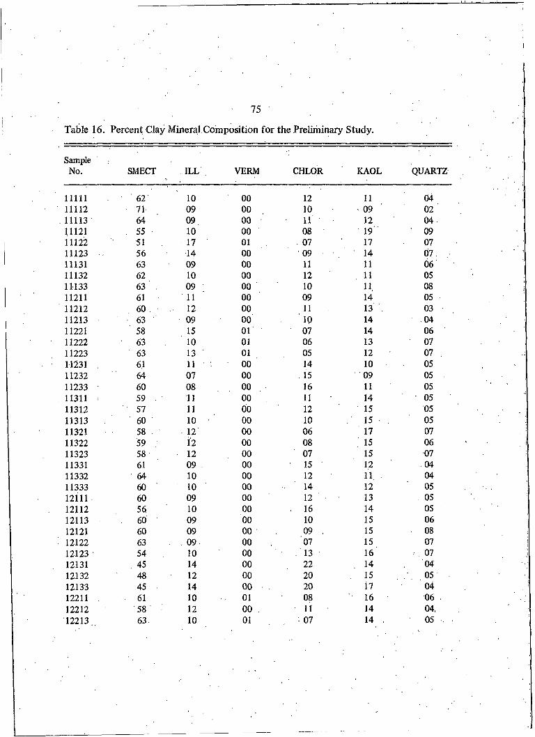
75

Table 16. Percent Clay Mineral Composition for the Preliminary Study.

SampleNo. SMECT ILL VERM CHLOR KAOL QUARTZ

11111 62 10 00 12 11 0411112 71 09 00 10 09 0211113 64 09. 00 11 12 0411121 . 55 ■ 10 00 08 19 0911122 51 17 ' 01 07 17 0711123 56 14 00 09 14 07 .11131 63 09 00 11 11 0611132 62 10 00 12 11 OS11133 63 . 09 00 10 11 0811211 61 11 00 09 14 0511212 60. 12 00 11 13 . 0311213 63 09 00 10 14 .0411221 58 15 01 07 14 0611222 63 10 01 06 13 0711223 63 13 01 05 12 07 .11231 6.1 11 00 14 10 0511232 64 07 00 . 15 09 0511233 60 08 00 16 11 0511311 : 59 . 11 00 11 14 OS11312 57 . 11 00 12 15 0511313 60 10 00 10 . 15 0511321 58 ■ ■ 12 00 06 17 0711322 59 . 12 00 08 . 15 0611323 58 12 00 07 15 0711331 61 09 00 15 12 0411332 64 10 00 12 11. 0411333 60 10 00 14 12 0512111 60 09 00 12 13 OS12)12 56 10 00 . 16 14 0512113 60 09 00 10 15 0612121 60 09 00 09 . 15 0812122 63 . 09 00 07 15 0712123 54 10 00 13 16 . 0712131 . 45 14 00 22 14 0412132 48 12 00 20 . 15 0512133 45 14 00 20 17 0412211 . 61 10 01 08 16 06 •12212 58 12 00 . 11 14 04,12213 63 10 01 07 14 . 05

76



12221 64 09 00 . 06 14 0612222 59 . . 10 00 06 .17 0812223' 60 10. 02 04 16 07.12231 66 09 00 11 11 0412232 67 10 00 09 10 0312233 . 66 08 00 12 10 0412311 61 11 00 09. 13 0512312 58 10 00 13 13 0512313 60 . io 00 10 14 0612321 61 11 04 04 14 0612322 61 ■ 11 01 04 16 . 0712323 60 09 00 08 15 0712331 69 06 00 12 . 09 . .0412332 66 . 07 00 12 10 0512333 68 . 08 00 10 10 0513111 67 . 09 00 10 12 . 02 .13112 67 08 00 Tl 11 02 -13113 64 11 00 . 1 2 10 0313121 62 . 07 00 06 17 0813122 59 09 00 09 17 0613123 57 08 00 09 17. 0813131 64 08 ob .20, 07 0113132 69 07 00 14 07 0213133 72 07 00 14 07 0113211 59 07 00 14 14 0613212 62 06 00 12 14 0613213 62 . 07 00 11 14 0613221 64 08 .01 05 14 0513222 64 • . 08 00 07 16 0613223 62 08 00 09 16 .0 613231 69 05 00 16 08 0313232 71 ' 05 00 13 08 0313233 68 06 00 16 07 0213311 58 07 00 17 • 13 0513312 60 07 00 13 13 07 .13313 • 57 09 00 17 12 05 .13321 62 07 00 08 17 0613322 62 08 00 06 . 17 0713323 61 09 01 05 17 0.7

77



13331 67 08 00 13 10 0313332 70 06 00 11 10 0313333 72 OS 00 10 10 0321111 00 41 00 26 29 0421112 00 39 00 24 30 0721113 00 37 00 23 33 0621121 00 33 00 14 37 1521122 00 35 00 14 37 1521123 00 36 00 14 37 1321131 00 37 00 25 30 0821132 00 35 00 28 29 0821133 00 41 00 28 26 0521211 00 35 00 21 32 1121212 00 39 00 21 33 0821213 00 39 00 21 31 0921221 00 43 00 10 36 1121222 00 41 00 11 37 1121223 00 41 00 10 36 1321231 00 37 00 21 33 1021232 00 43 00 21 29 0721233 00 39 00 21 33 0721311 00 30 00 19 38 1221312 00 35 00 16 37 1321313 00 37 00 15 36 1221321 00 38 00 11 39 1121322 00 37 00 13 37 1321323 00 38 00 11 . 38. 1321331 00 48 00 18 29 OS21332 00 48 00 16 31 OS21333 00 43 00 14 34 0822111 00 57 00 14 28 0122112 00 41 00 18 33 0822113 00 42 00 14 35 0922121 00 41 00 08 42 0922122 00 40 00 10 40 1122123 00 40 00 08 41 1122131 00 . 42 00 19 34 0522132 00 40 00 20 32 0722133 00 42 00 19 31 08

78



22211 00 42 00 21 30 0722212 00 36 00 18 35 1122213 00 40 00 , 22 30 0922221 • 00 40 00 09 38 1322222 00 40 00 09 38 1322223 00 39 00 10 38 1322231 00 44 00 16 33 0622232 00 47 00 17 32 0422233 00 41 00 17 35 0722311 00 39 00 17 32 1122312 00 35 00 17 36 1222313 00 35 00 19 33 1422321 00 39 00 11 37 1422322 00 45 00 09 34 1222323 00 39 00 10 38 1322331 00 39 00 16 37 0822332 00 39 00 18 34 0922333 00 40 00 17 33 1023111 00 42 00 17 30 1123112 00 43 00 15 32 1023113 00 41 00 18 30 1123121 00 39 00 12 33 1523122 00 41 00 10 34 1523123 00 41 00 12 34 1323131 00 44 00 19 29 0823132 00 . 42 00 20 29 0923133 00 42, 00 23 29 0723211 00 43: 00 19 32 0723212 00 45 00 18 30 0823213 00 48 00 16 30 0623221 00 42 00 09 34 1423222 00 45 00 08 33 1423223 00 43 00 12 33 1223231 00 35 00 18 29 1723232 00 34 00 25 27 1423233 00 35 00 24 27 1523311 00 ' 38 00 15 30 1623312 00 39 00 14 28 1823313 00 39 00 15 29 17

79



23321 00 35 00 14 34 1623322 00 36 00 12 35 1723323 00 39 00 12 31 1823331 00 49 00 13 29 0923332 00 48 00 18 29 0523333 00 49 00 14 31 0631111 '15 30 04 12 30 0931112 16 32 01 13 31 0731113 18 31 OS 13 25 0831121 14 33 06 09 28 11 .31122 13 ' 36 03 08 28 1131123 15 36 00 08 29 1131131 15 39 17 09 18 0331132 15 28 18 07 26 0731133 16. 38 10 09 25 0331211 20 32 00 14 25 0831212 17 33 02 14 25 0831213 18 31 07 13 23 0831221 14 37 09 OS 26 0831222 12 38 07 06 29 0931223 12 36 02 13 28 0831231 21 33 01 16 23 0731232 22 30 07 11 . 25 0631233 24 27 08 13 21 0731311 13 33 00 16 31 0731312 14 32 04 12 30 0831313 15 33 00 14 31 0731321 14 37 04 06 30 1031322 14 37 00 11 29 0931323 10 33 13 05 .31 . 0831331 20 30 11 09 23. .0631332 20 29 12 07 26 0631333 20 31 10 07 27 OS32111 14 35 . os 09 30 07.32112 14 44 02 12 ' 25 03.32113 13 41 03 09 29 OS32121 11 37 03 08 32 09 .32122 10 37 , OS 07 32 0932123 12 33 . 04 07 34 10

80



32131 16 41 07 08 25 0332132 21 35 02 10 27 0532133 17 36 07 12 24 0432211 12 41 02 11 29 0532212 13 46 01 09 28 0332213 14 44 06 07 26 0232221 13 37 04 07 33 06.32222 12 37 05 06 34 0632223 09 47 01 07 32 0432231 18 37 08 08 25 0432232 19 34 04 09 27 0632233 18 36 07 09 25 . 0532311 13 43 00 13 27 0532312 12 41 03 10 29 0532313 13 39 00 15 27 OS32321 13 35 00 11 33 0932322 11 36 03 07 34 0932323 13 38 00 08 33 .0932331 17 36 05 08 30 0432332 17 36 08 10 24 OS32333 17 35 11 08 24 OS33111 14 44 02 12 21 0733112 15 44 00 15 20 0733113 19 37 02 14 21 0833121 11 42 03 07 25 1233122 05 40 01 10 25 1033123 13 33 00 09 31 1433131 . 26 34 03 10 19 0833132 27 32 02 10 21 0833133 22 30 08 11 23 0733211 14 44 03 12 21 0633212 15 40 01 12 25 0733213 14 40 01 16 22 0733221 12 35, 00 11 30 1233222 12 43 ; 02 10 24 09 .33223 .11 46 00 10 . 2 5 , 0933231 18 34 00 21 20 0733232 20 36 00 17 20 0833233 17 38 00 16 21 07

81



33311 13 42 02 09 27 0633312 13 42 06 07 26 0533313 13 38 06 08 28 0833321 11 38 05 04 34 0833322 12 40 07 04 30 0833323 13 39 03 07 38 0933331 20 37. 07 07 . 22 0933332 18 37 02 09 27 0533333 17 37 09 10 22 06

82

Table 17. ANOVA for Main Effects on the 17A Peak (MgEG) for All Three Soils Studied-Preliminary Study

SoxirceDegrees of Freedom

Sum of Squares

MeanSquares

VarianceComponent F-Value

Total 242 1108.160 4.579 6.635Soils 2 972.767 . 486.383 5.997 780.43*Clay Sep. 6 3.739 0.623 -0.028 0.45Slide 18 24.946 1.386 -0.045 0.77Field/Slide 54 96.770 1.792 0.577 29.21*Error 162 9.937 - 0.061 0.061


Table 18. ANOVA for Main Effects on the IOA Peak (MgEG) for AU Three Soils Studied- Preliminary Study

SourceDegrees of Freedom

SumofSquares

MeanSquares


Total 242 8.243 0.034 0.047Soils 2 6.294 3.147 0.038 81.14*Clay Sep. 6 0.233 0.039 0.001 2.08Slide . 18 0.336 0.019 0.000 0.97Field/Slide 54 1.028 0.019 0.006 8.77*Error 162 0.353 0.002 0.002


I

83

Table 19. ANOVA for Main Effectsonthe 14A Peak (MgEG) for AU Three SoUs Studied—PreUminary Study


Sum of Squares

MeanSquares


Total 242 4.991 0.021 0.028Soils 2 2.043 1.021 0.012 16.34*Clay Sep. 6 0.375 0.063 0.002 10.64*SUde 18 0.106 0.006 -0.003 0.17Field/SUde 54 1.854 0.034 0.010 9.07*Enor 162 0.613 . 0,004 0.004


Table 20. ANOVA for Main Effects on the 14A Peak (K350) for AU Three SoUs Studied— PreUminary Study


SumofSquares

MeanSquares


Total 242 5.170 0.021 0.027Soils 2 0.550 * 0.275 0.003 18.45*Clay Sep. 6 0.089 0.015 0.000 0.59SUde 18 0.451 0.025 -0.004 0.38Field/SUde 54 3.534 0.065 0.021 19.45*Enor 162 0.545 0.003 0.003


84

Table 21. ANOVA for Main Effects on the 7A Peak (MgEG) for All Three Soils Studied-Preliminary Study


Sum of Squares

MeanSquares


Total 242 134.659 0.143 0.185Soils 2 20.615 10.307 0.121 21.82*Clay Sep. 6 2.835 0.472 0.005 1.44Slide 18 5.903 0.328 0.028 4.16*Field/Slide 54 4.259 0.079 0.024 12.20*Error 162 1.047 0.006 0.006


Table 22. ANOVA for Main Effects on the 7A Peak (K350) for All Three Soils Studied- Preliminary Study


Sum of Squares

MeanSquares


Total 242 44.365 0.183 0.224Soils 2 20.073 10.036 0.102 5.76*Clay Sep. 6 10.450 1.742 0.056 7.67*Slide 18 4.087 0.227 0.005 1.28Field/Slide 54 9.594 0.178 0.059 177.52*Error 162 0.162 0.001 0.001


85

Table 23. ANOVA for Main Effects on the 3.5 A Peak (MgEG) for All Three Soils Studied-Preliminary Study


Sum of Squares

MeanSquares


Total 242 12.311 0.051 0.068Soils 2 7.397 3.698 0.045 63.14*Clay Sep. 6 0.351 0.059 -0.002 0.49Slide 18 2.137 0.119 0.100 3.75*Field/Slide 54 1.711 0.032 0.009 7.19*Error 162 0.714 0.004 0.004


Table 24. ANOVA for Main Effects on the 3.3 A Peak (MgEG) for All Three Soils Studied- Preliminary Study


Sum of Squares

MeanSquares


Total 242 10.449 0.043 0.055Soils 2 5.913 2,956 0.034 16.96*Clay Sep. 6 1.046 0.174 0.003 2.18Slide 18 1.441 0.080 0.005 2.49*Field/Slide 54 1.734 0.032 0.010 16.49*Error . 162 0.315 0.002 . 0.002

* „ significant at a = 0.05

86

Table 25. ANOVA of Percent Smectite Composition for All Three Soils Studied—Preliminary Study


Sum of Squares

MeanSquares


Total 242 16.925 0.070 0.104Soil 2 16.596 8.298 0.102 1463.49*Clay Sep. 6 0.034 0.006 0.000 1.85Slide 18 0.055 0.003 0.000 0.82Field/Slide 54 0.201 0.004 0.001 15.28*Error 162 0.039 0.000 0.000


Table 26. ANOVA of Percent Illite Composition for All Three Soils Studied—Preliminary Study


Sum of Squares

MeanSquares


Total 242 5.003 0.021 0.030Soil 2 4.656 2.328 0.029 180.88*Clay Sep. 6 0.077 0.013 0.000 11.92*Slide 18 0.019 0.001 0.000 0.37Field/Slide 54 0.158 0.003 0.001 5.09*Error 162 0.093 0.001 0.001


87

Table 27. ANOVA of Percent Vermiculite Composition for All Three Soils Studied—Preliminary Study


Sum of Squares

MeanSquare

. Variance Component F-Value

Total 242 0.219 0.001 0.001Soil 2 0.090 0.045 0.001 18.58*Clay Sep. 6 0.015 0.002 0.000 3.55*Slide 18 0.012 0.001 0.000 0.63Field/Slide 54 0.059 0.001 0.000 4.06*Error 162 0.043 0.000 0.000


Table 28. ANOVA of Percent Chlorite Composition for All Three Soils Studied—Preliminary Study


Sum of Squares

MeanSquares


Total 242 0.579 0.002 0.003SoU 2 0.185 0.093 0.001 29.77*Clay Sep. 6 . 0.019 0.003 0.000 0.83SUde 18 0.067 0.004 0.000 0.77Field/SUde 54 0.261 0.005 0.001 16.66*Error 162 0.047 0.000 0.000


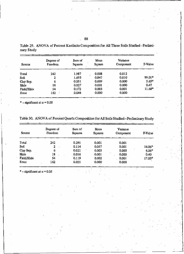
88

Table 29. ANOVA of Percent Kaolinite Composition for All Three Soils Studied—Preliminary Study


Sum of Squares

MeanSquare


Total 242 1.987 0.008 0.012Soil 2 1.693 0.847 0.010 99.01*Clay Sep. 6 0.051 0.009 0.000 5.65*Slide 18 0.027 0.001 0.000 0.47Field/Slide 54 0.172 0.003 0.001 11.68*Error 162 ' 0.044 0.000 0.000


Table 30. ANOVA of Percent Quartz Composition for AU Soils Studied—Preliminary Study


Sum of Squares

MeanSquares


Total 242 0.291 0.001 0.001Soil 2 ■ 0.114 0.057 0.001 16.06*Clay Sep. 6 0.021 0.003 0.000 4,06*Slide 18 . 0.016 0.001 0.000 0.40Field/Slide 54 0.119 0.002 0.001 17.03*Error 162 0.021 0.000 0.000


Table 3 1. Complete Peak Area Measurements (in.2 ) for the Main Study-

SampleNo. 17AMgEG IOAMgEG HAMgEG I4AK350 7AK350 7AK500 7AMgEG 3.5 A MgEG 3.3AMgEG

11 4.45 0.35 0.52 0.59 0.18 0.00 0.73 0.47 0.4712 5.65 0.38 0.60 0.62 0.26 0.00 0.65 0.41 0.4421 2.40 0.39 0.59 0.41 0.27 0.00 0.63 0.43 0.6722 2.50 0.33 0.34 0.49 0.48 0.00 0.36 0.37 0.5831 1.39 0.23 0.19 0.42 0.25 0.00 0.36 0.38 0.6132 2.09 0.28 0.19 0.54 0.27 0.00 0.48 0.5441 2.07 0.14 0.21 0.44 0.39 0.00 0.43 0.23 0.3642 1.85 0.12 0.18 0.52 0.18 0.00 0.59 0.50SI 5.17 0.09 0.25 0.33 0.73 0.00 0.61 0.33 0.3352 2.89 0.06 0.17 0.48 0.21 0.00 0.60 0.4261 8.56 . 0.22 0.72 0.66 0.39 0.00 1.38 0.59 0.5662 4.27 0.14 0.30 0.62 0.47 0.00 0.76 0.5571 15.53 0.28 0.00 0.75 0.22 0.00 1.01 0.52 0.7372 7.20 0.16 0.35 0.59 0.13 0.00 0.66 0.37 0.65SI 5.04 0.81 1.29 0.90 0.29 0.00 2.00 1.20 1.1082 3.19 0.46 - 0.63 0.63 0.28 0.00 1.32 0.71 0.7291 0.93 0.79 0.42 0.80 0.45 0.00 1.98 0.91 0.6292 0.91 0.68 0.60 0.88 0.53 0.00 1.85 1.31 0.78

IOl 0.35 0.53 0.20 0.69 0.46 0.00 1.32 1.05 1.08102 1.21 0.84 0.69 0.61 0.44 0.00 1.50 1.01 0.91II I 0.22 0.99 0.31 0.89 0.57 0.00 2.51 1.35 0.87

.112 0.51 0.89 0.49 0.60 2.11 0.00 2.73 1.40 0.85121 0.13 1.21 0.31 0.59 1.83 0.00 3.20 1.76 1.04122 0.31 0.72 0.49 0.69 1.54 0.00 1.80 1.20 0.74131 0.00 1,01 0.35 0.72 1.64 0.00 2.81 2.24 1.32132 0.00 0.71 0.35 0.58 1.65 0.14 2.55 1.15 0.75141 4.61 0.40 0.35 0.42 0.36 0.00 0.72 0.50 0.53142 4.10 0.38 0.22 0.47 0.44 0.00 0.55 0.36 0.38151 5.52 0.14 0.35 0.55 0.14 0.00 0.44 0.27 0.44


SampleNo. 17AMgEG IOAMgEG 14AMgEG 14AK350 7AK350 7AK500 7AMgEG 3.5 A MgEG 3.3A MgEG

152 6.80 0.17 O.O0 0.41 0.12 0.00 0.41 0.27 0.37161 4.51 0.11 0.00 1.17 0.19 0.00. 0.29 0.30 0.70162 14.61 0.19 0.00 0:52 0.24 0.00 0.42 0.21 0.54171 6.30 0.11 0.00 0.65 0.21 0.00 0.22 0.21 0.55-172 15.93 0.28 O.O0 0.79 0.22 0.00 0.55 0.35 1.06181 2.68 0.16 0.00 - 0.78 0.16 0.00 0.15 . 0.27 0.46182 13.30 0.35 0.00 0.70 0.11 0.00 0.48 0.34 1.03191 2.57 . 0.19 0.00 0.68 0.13 0.00 0.23 0.68192 16.40 0.38 0.00 0.84 0.13 o.oo 0.51 0.35 0.88201 8.30 0.57 0.00 1.15 0.00 0.00 0.87 0.61 1.03202 7.57 0.63 0.00 1.31 0.00 0.00 0.93 0.43 0.65211 6.25 0.60 0.00 0.91 0.12 0.00 0.97 0.73 1.17212 9.71 . 0.95 0.00 1.24 0.00 0.00 1.01 0.65 0.87221 2.59 0.28 0.00 1.08 0.60 0.00 0.49 0.45 0.72222 11.00 0.53 0.00 0.68 0.14 0.00 1.01 . 0.67 0.99231 8.50 0.22 0.00 1.13 0.53 0.00 0.52 0.75232 4.59 0.16 0.00 0.68 0.16 0.00 0.38 0.63241 11.00 0.12 0.00 0.79 0.34 0.00 0.39 0.77

. 242 3.22 0.11 0.00 0.73 0.16 0.00 0.29 0.74251 8.50 0.34 0.00 0.99 0.19 0.00 0.79 0.62252 6.70 0.30 0.00 1.01 0.08 0.00 0.95 0.47 0.62261 8.90 0.50 0.00 1.20 0.13 0.00 1.02 0.46 0.44262 8.28 0.52 0.00 1.07 0.15 0.00 1.33 0.71 0.71271 8.87 0.87 0.00 0.80 3.60 0.00 4.13 2;03 1.21272 8.16 0.88 0.00 0.74 2.84 0.00 4.16 2.11 0.91281 1.22 1.51 1.18 0.92 0.82 0.00 3.30 2.36 2.10282 1.57 1.33 0.63 0.69 1.05 0.00 3.24 2.62 1.90291 0.00 1.59 0.41 0.13 4.72 0.00 5.59 3.78 1.47292 0.00 1.50 0.23 0.21 5.63 0.00 5.06 3.13 1.15


SampleNo. 17AMgEG IOAMgEG 14AMgEG 14AK350 7AK350 7AK500 TAMgEG. 3.5AMgEG 3.3 A MgEG

301 0.00 LlO 0.00 0.00 4.63 0.00 6.06 3.19 0.73302 0.00 0.57 0.00 . 0.16 2.46 0.00 2.44 1.38 0.35311 0.00 1.37 0.00 0.23 0.94 0.00 5.03 2.59 1.20312 0.00 1.61 0.00 0.21 1.79 0.00 4.59 2.64 1.09321 0.00 . 2.03 0.44 0.49 2.10 0.00 3.03 2.15 1.91322 0.00 2.05 0:62 0.61 2.97 0.00 3.56 2.05 1.61331 0.00 1.65 0.39 0.58 2.03 0.00 3.63 2.31 1.60332 0.00 1.91 0.49 0.71 2.53 0.00 3.75 2.07 1.54341 0.00 1.97 0.56 0.56 3.25 0.00 3.47 1.91 1.53342 0.00 1.92 0.54 0.66 1.24 0.00 3.22 2.11 1.33351 0.00 1.15 0.00 0.00 1.67 0.00 2.23 1.42 0.89352 0.00 „ 0.76 0.00 0.00 0.68 0.00 1.93 1.03 0.71361 0.00' 1.69 0.00 0.00 3.97 0.00 5.22 2.75 1.00362 0.00 1.40 0.44 0.28 1.12 0.00 4.69 2.69 1.11371 0.00 1.20 0.00 . 0.00 1.04 0.00 4.78 2.49 0.89372 0.00 1.29 0.00 0.22 • 0.81 0.00 4.95 2.41 0.90381 8.53 0.62 0.00 0.55 0.79 0.00 1.44 1.03 1.40382 8.45 0.58 0.00 0.49 0.61 0.00 1.33 0.94 1.13391 6.60 0.88 0.95 0.54 0.42 0.00 1.65 1.49 1.51392 5.00 0.69 1.05 0.81 0.49 0.00 1.60 1.31 1.67401 5.85 0.44 0.00 0.45 0.20 0.00 0.82 0.55 0.47402 5.12 0.53 0.00 0.31 . 0.23 0.00 0.92 0.48 0.56411 5.82 0.53 0.80 0.34 0.11 0.00 0.89 0.49 0.58412 6.24 0.63 0.96 0.30 0.32 0.00 0.97 0.73 0.69421 0.95 1.26 0.45 0.49 1.15 0.00 2.40 1.43 1.19422 . 1.27 1.11 0.45 0.34 1.69 0.00 2.43 1.33 1.10431 0.00 1.30 0.48 0.40 3.36 0.00 2.66 1.61 1.24432 0.00 1.58 0.41 0.41 0.96 0.00 2.60 1.39 1.00441 ODQ 1.34 0.43 0.57 3.13 0.00 3.97 2.15 1.07


SampleNo. 17AMgEG IOAMgEG 14AMgEG 14AK350 7AK350 7AK500 7AMgEG 3.5A MgEG 3.3A MgEG

442 0.00 1.40 0.48 0.54 2.63 0.00 3.81 2.06 1.08451 0.00 0.64 0.00 0.00 0.29 0.00 1.90 1.24 0.95452 0.00 0.68 0.00 0.18 0.24 0.00 1.90 1.21 1.01461 0.00 0.84 0.57 0.81 1.13 0.00 7.40 4.63 0.86462 0.00 0:77 0.55 0.71 1.56 0.00 7.60 4.03 0:80471 0.00 1.21 0.62 0.49 4.25 0.00 7.50 5.37 1.45472 0.00 1.00 0.58 0.54 4.06 0.00 7.25 3.80 1.10481 0.00 1.30 0.63 0.56 4.06 0.00 6.55 4.59 1.39482 0.00 1.28 0.54 0.41 2.33 0.00 6.35 3.75 1.20491 0.00 1.35 0.54 0.45 1.14 0.00 3.59 2.81 1.37492 0.00 1.39 0.54 0.59 0.87 0.00 4.25 2.81 1.52501 1.53 0.70 0.00 0.39 0.10 0.00 1.75 1.65 1.69502 2.27 0.90 0.00 0.27 0.14 0.00 2.21 1.57 1.76

VOto

93

Table 32. Complete Data Table for Modification IV

PSM PIL PVM PCA PKA PQU ECEC LCEC TKIL8

I 54.3 15.7 0.0 13.1 15.0 2.0 62.70 56.25 152 39.7 22.6 0.0 14.1 17.9 5.6 50.43 47.50 153 35.2 21.2 0.0 18.3 17.1 8.2 46.62' 42.50 144 43.3 10.7 0.0 17.1 21.7 7.1 52,18 42.50 135 58.9 4.7 0.0 12.7 18.7 5.0 64.88 51.25 86 57.3 6.7 0.0 12.4 19.3 4.1 63.71 46.25 117 70.1 5.7 0.0 9.2 11.1 3.7 74.85 62.50 88 34.4 21.0 0.0 13.2 27.8 3.7 45.18 32.50 209 9.6 30.9 0.0 17.7 40:2 1.6 25.03 21.25 27

10 9.0 33.3 0.0 16.2 35.0 6.3 24.36 20.00 3011 3.2 34.3 0.0 13.4 47.6 1.4 19.02 20.00 2712 1.6 36.7 0.0 . 12.7 47.3 . 1.7 17.76 17.50 2713 0.0 33.0 0.0 12.6 50.7 3.6 15.52 17.50 2914 51.3 19.6 0.0 11.3 15.8 1.9 60.36 40.00 1915 67.4 7.6 0.0 11.6 10.2 3.5 73.02 58.75 . 1416 75.6 4.3 0.0 13.1 4.7 2.2 80.37 72.50 1117 72.3 5.5 0.0 11.8 5.4 4.9 77.17 62.50 1118 72.8 8.1 0.0 9.1 5.6 4.5 77.64 63.75 1719 37.7 15.2 0.0 27.2 9.2 10.7 49.25 42.50 1920 48.7 17.5 0.0 17.9 13.1 2.8 58.65 48.75 2021 46.8 21.0 0.0 14.8 13.9 3.4 56.98 43.75 2322 59.0 12.6 0.0 12.8 12.0 3.5 66.38 48.75 2223 57.6 8.1 0.0 18.8 9.6 5.9 65.20 46.25 1724 47.6 6.6 0.0 24.3 10.7 10.8 56.38 53.75 1525 54.5 11.1 0.0 16.7 14.6 3.1 62.69 47.50 1826 52.0 14.2 0.0 15.8 16.4 1.5 60.85 37.50 2627 36.0 16.3 0.0 7.2 38.6 1.8 45.05 28.75 2228 12.2 35.0 0.0 10.1 37.3 5.4 26.51 22.50 2929 0.0 35.1 1.9 1.7 60.4 0.8 17.30 17.50 2430 0.0 28.6 0.0 2.2 69.2 0.0 13.24 12.50 2131 0.0 37.0 0.0 2.7 59.7 0.5 14.71 17.50 2332 0.0 50.2 0.0 7.4 40.5 1.9 17.68 12.50 3733 0.0 44.3 0.0 8.0 46.1 1.5 16.81 12.50 3834 0.0 49.5 0.0 7.7 42.5 0.2 17.72 10.00 3335 0.0 46.9 0.0 0.0 51.9 1.1 15.90 23.75 2736 0.0 36.0 3.5 2.4 57.9 0.2 20.46 17.50 2437 0.0 33.0 0.0 1.4 65.2 0.0 13.91 17.50 2438 53.2 16.0 0.0 6.9 18.4 5.4 60.52 47,40 1939 33.7 20.5 0.0 7.6 31.5 6.5 43.43 42.50 2240 52.6 20.1 0.0 7.8 18.0 1.5 61.08 47.50 20



41 49.6 19.0 9.1 5.3 15.3 1.6 72.95 38.75 2142 9.1 40.3 0.9 6.3 41.7 1.6 25.71 17.50 3043 0.0 47.6 0.0 7.2 44.1 1.1 17.24 12.50 3344 0.0 38.0 0.0 7.7 53.9 0.3 15.76 12.50 3345 0.0 35.9 0.0 6.0 51.6 6.5 14.72 31.25 2346 0.0 16.1 0.0 7.6 75.1 1.1 11.97 20.00 1947 0.0 20.6 0.6 5.2 71.1 2.5 13.24 17.50 2048 0.0 26.4 1.0 4.9 66.0 1.7 14.99 17.50 2049 0.0 37.2 0.0 6.9 53.0 2.8 15.33 12.50 3450 14.3 30.2 0.0 7.0 37.6 10.9 26.85 30.00 24

95

Table 33. Complete Data Table for Modification V


I 47.2 13.7 0.0 11.3 26.0 1.7 55.58 56.25 152 33.7 19.2 0.0 12.0 30.3 4.7 44.07 47.50 153 30.0 18.2 0.0 15.6 29.2 7.0 40.93 42.50 144 35.6 8.8 0:0 14.1 35.6 5.8 44.33 42.50 135 49.8 3.9 0.0 10.6 31.3 4.2 56.04 51.25 86 48.0 5.6 0.0 10.4 32.4 3.5 54.68 46.25 117 63.2 5.2 0.0 8.2 20.1 3.3 68.23 62.50 88 26.9 16.4 o:o 10.3 43.5 2.8 37.12 32.50 209 6.9 22.0 0.0 12.6 57.4 LI 20.17 21.25 27

10 6.7 24.8 . 0.0 11.9 51.9 4.7 20.17 20.00 3011 2.2 23.2 o:o 9.1 64.5 1.0 15.47 20.00 2712 1.1 24.9 0.0 8.6 64.2 1.2 14.63 17.50 2713 0.0 22.0 0.0 8.3 67.3 2.4 13.01 17.50 2914 44.3 16.9 o.o . 9.7 27.2 1.7 53.23 40.00 1915 61.2 6.7 0.0 10.5 18.5 3.1 67.04 58.75 1416 72.2 4.1 0.0 12.6 9.0 2.1 77.14 72.50 1117 68.5 5.2 0.0 11.2 10.3 4.7 73.58 62.50 1118 68.9 7.7 0.0 8.6 10.6 4.2 73.91 63.75 1719 34.6 13.9 0.0 24.9 16.8 9.8 45.84 42.50 1920 43.0 15.5 0.0 15.8 23.1 2.5 52.76 48.75 2021 41.2 18.5 0.0 13.0 24.3 3.0 51.08 43.75 2322 52.7 11.3 0.0 11.5 21.5 3.1 60.18 48:75 2223 52.5 . 7.4 0.0 17.1 17.4 5.4 60.19 46.25 1724 42.9 6.0 0.0 21.9 19.3 9.8 51.67 53.75 1525 47.6 9.8 0.0 14.6 25.4 2.6 55.81 47.50 1826 44.7 12.3 o,o 13.6 28.1 1.3 53.49 37.50 2627 26.0 11.8 0.0 5.1 55.7 1.3 34.71 28.75 2228 8.9 25.4 0.0 7.3 54.3 3.9 21.52 22.50 2929 0.0 21.9 1.2 1.0 75.3 0.5 13.79 17.50 2430 0.0 16.9 . 0.0 1.3 81.8 0.0 11.11 12.50 2131 0.0 23.2 0.0 1.7 74.7 0.3 12.22 17.50 2332 0.0 35.7 0.0 5.2 57.6 1.3 14.89 12.50 3733 0.0 30.3 0.0 5.5 63.1 1.0 14.03 12.50 3834 0.0 34.7 0.0 5.4 59.7 0.1 14.83 10.00 3335 0.0 30.9 0.0 0.0 68.3 0.7 13.22 23.75 2736 0:0 22.8 2.3 1.5 73.4 0.1 15.88 17.50 2437 0.0 20.2 0.0 0.8 78.9 0.0 11.58 17.50 2438 44.9 13.5 0.0 5.8 31.2 4.5 52.32 47.40 1939 25.7 15,6 0.0 5.7 47.9 5.0 34.97 42.50 .2240 44.6 16.9 0.0 6.6 30.4 1.3 52.95 47.50 20

96



41 43.1 16.5 7.9 4.6 26.6 1.4 64.27 38.75 2142 6.4 28.5 0.7 4.5 58.9 1.1 20.60 17.50 3043 0.0 33.1 0.0 4.9 61.2 0.8 14.41 12.50 3344 0.0 24.7 0.0 5.0 70.1 0.2 13.04 12.50 3345 0.0 23.6 0.0 3.9 68.0 4.3 12.42 31.25 2346 0.0 9.2 0.0 4.3 85.8 0.6 10.28 20.00 1947 0.0 12.0 0.3 3.0 83.1 1.4 11.07 17.50 2048 0.0 15.9 0.6 3.0 79.5 1.0 12.16 17.50 2049 0.0 24.3 0.0 4.5 69.3 1.9 12.81 12.50 3450 10.4 22.0 0.0 5.1 54.5 . 7.9 21.71 30.00 . 24

97

Table 34. Complete Data Table for Modification IX.


I 48.6 17.7 0.0 14.6 16.8 2.2 58.11 56.25 152 34.5 ' 24.6 0.0 15.4 19.4 6.1 46.18 47.50 153 30.3 22.8 0.0 19.7 18.4 8.8 42.52 42.50 144 37.9 11.7 0.0 18.8 23.8 7.8 47.62 42.50 135 59.3 5.7 0.0 13.8 17.5 3.7 65.65 51.25 86 51.8 7.5 0.0 14.0 21.9 4.7 59.08 46.25 117 65.3 6.7 0.0 10.6 12.9 4.3 70.81 62.50 88 29.5 22.5 0.0 14.1 29.9 3.9 41.12 32.50 209 7.8 31.4 0.0 18.0 41.0 1.6 23.54 21.25 27

10 7.4 34.0 0.0 16.5 35.7 6.4 23.00 20.00 3011 2.6 34.5 0.0 13.5 47.9 1.4 18.52 20.00 2712 1.3 36.8 0.0 12.7 47.5 1.7 17.51 17.50 2713 0.0 33.0 0.0 12.6 50.7 3.6 15.52 17.50 2914 45.8 21.8 0.0 12.5 17.6 2.1 55.86 40.00 1915 62.3 8.6 0.0 13.4 11.8 4.0 68.81 58.75 1416 71.3 5.0 0.0 15.5 5.6 2.6 76.93 72.50 1117 67.6 6.4 0.0 13.7 6.3 5.8 73.31 62.50 1118 68.1 9.5 0.0 10.6 6.5 5.2 73.75 63.75 1719 32.7 16.4 0.0 29.4 9.9 11.6 45.17 42.50 1920 43.2 19.3 0.0 19.8 14.6 3.1 54.18 48.75 2021 41.4 23.2 0.0 16.3 . 15.4 3.7 52.58 43.75 2322 53.5 14.3 0.0 14.6 13.6 4.0 61.89 48.75 2223 52.1 9.1 0.0 21.2 10.9 6.7 60.70 46.25 1724 42.1 , 7.3 0.0 26.8 . 11.8 11.9 51.81 53.75 1525 49.0 12.5 0.0 18.7 16.3 3.4 58.18 . 47.50 1826 46.5 15.9 0.0 17.7 18.3 1.7 56.33 .37.50 2627 31.0 17.5 0.0 7.7 41.6 2.0 40.75 28.75 2228 10.0 35.9 0.0 10.4 38.2 5.6 24.72 22.50 2929 0.0 35.1 1.9 1.7 60.4 0.8 17.30 17.50 2430 0.0 28.6 0.0 2.2 69.2 0.0 13.24 12.50 2131 0.0 37.0 0.0 2.7 59.7 0.5 14.71 17.50 2332 0.0 50.2 0.0 7.4 40.5 1.9 17.68 12.50 37;33 0.0 44.2 0.0 8.0 46.1 1.5 16.81 12.50 3834 0.0 49.5 0.0 . 7.7 42.5 0.2 17.72 10.00 3335 0.0 46.9 0.0 0.0 51.9 1.1 15.90 23.75 2736 0.0 36.0 3.5 2.4 57.9 0.2 20.46 17.50 2437 OO 33.3 0.0 1.4 65.2 0.0 13.91 17.50 2438 47.6 17.9 0.0 7.7 20.6 6.0 55.79 47.40 1939 28.9 22.0 0.0 8.1 33.8 7.0 39.34 42.50 2240 47.0 22.4 0.0 817 20.0 1.7 56.48 47.50 20

98



41 44.0 21.2 10.1 5.9 16.9 1.9 69.95 38.75 2142 7.9 41.0 1.0 6.5 42.5 1.6 24.47 17.50 3043 0.0 47.6 0.0 7.2 44.1 1.1 17.24 12.50 3344 0.0 38.0 0.0 7.7 53.9 0.3 15.76 12.50 3345 0.0 35.9 0.0 6.0 51.6 6.5 14.72 31.25 2346 0.0 16.1 0.0 7.6 75.1 1.1 11.97 20.00 1947 0.0 20.6 0.6 5.2 71.1 2.5 13.24 17.50 2048 0.0 26.4 1.0 4.9 66.0 1.7 14.99 17.50 2049 0.0 37.2 0.0 6.9 53.0 2.8 15.33 12.50 3450 11.8 31.2 0.0 7.2 38.6 11.1 24.72 30.00 24

99

Table 35.. Complete Data Table for Modification X


I 41.7 15.1 0.0 12.5 28.7 1.9 50.95 56.25 152 28.9 20.6 0.0 12.9 32.5 5.0 40.01 47.50 153 25.6 19.3 0.0 16.6 31.0 7.4 37.17 42.50 144 30.8 9.5 0.0 15.2 38.3 6.3 40.1 i 42.50 135 50.5 4.9 0.0 11.7 29.8 3.1 57.10 51.25 86 42.5 6.1 0.0 11.5 35.9 3.8 49.92 46.25 117 57.9 5.9 0.0 . 9.5 22.9 3.8 63.66 62.50 88 22.7 17.3 0.0 10.9 46.0 . 3.0 33.49 32.50 209 5.6 22.3 0.0 12.8 58.2 1.1 19.05 21.25 27

10 5.5 25.0 0.0 12.1 ... 52.6 4.7 19.09 20.00 3011 1.7 23.3 0.0 9.1 64.8 1.0 15.07 20.00 2712 0.8 25.0 0.0 8.6 64.2 1.2 14.43 17.50 2713 0.0 22.0 0.0 8.3 67.3 2.4 13.01 17.50 2914 38.9 18.5 0.0 10.7 29.9 1.8 48.65 40.00 1915 55.8 7.6 0.0 11.9 21.1 3.6 62.44 58.75 1416 67.5 4.8 0.0 14.7 10.5 2.5 73.27 72.50 1117 63.6 . 6.0 0.0 13.0 11.9 5.4 69.43 62.50 11.18 63.9 8.9 0.0 10.0 12.3 4.9 69.71 63.75 1719 29.7 14.9 0.0 26.7 . 18.1 , 10.6 41.76 42.50 1920 37.7 .16.9 0.0 17.4 25.3 2.7 48.39 48.75 2021 . 35.9 20.1 0.0 14.1 26.5 3.2 . 46.71 43.75 2322 47.1 12.6 0.0 12.8 ' 24.0 3.5 . 55.44 48.75 2223 47.0 8.2 0.0 19.2 19.5 6.0 55.57 46.25 1724 37.7 6.5 0.0 23.9 21.1 10.7 47.18 53.75 1525 42.2 10.8 0.0 16.0 28.0 3.0 51.20 47.50 1826 39.3 13.4 0.0 15.0 30.8 1.4 48.91 37.50 2627 22.0 12.4 0.0 5.4 58.7 1.4 31.15 28.75 2228 7.2 25.9 0.0 7.5 55.3 4.0 20.05 22.50 2929 0.0 21.9 1,2 1.0 75.3 0.5 13.79 17.50 2430 0.0 16.9 6,0 1.3 81.8 0.0 11.11 12.50 2131 0.0 23.2 0.0 1.7 74.7 0.3 12.22 17.50 2332 0.0 35.7 0.0 5.2 57.6 1.3 14.89 12.50 3733 0.0 30.3 0.0 5.5 63.1 1.0 . 14.03 12.50 3834 0.0 34.7 0.0 5.4 59.7 0.1 14.83 10.00 3335 0.0 30.9 0.0 0.0 68.3 0.7 13.22 23.75 2736 0.0 22.8 2.3 1.5 73.4 0.1 15.88 17.50 2437 0.0 20.2 0.0 * 0.8 78.9 0.0 11.58 17.50 2438 39.5 14.8 0.0 6.4 34.2 5.0 47.60 47.40 1939 21.7 16.4 0.0 6.1 50.5 5.3 31.48 42.50 2240 39.2 18.6 0.0 7.3 33.4 1.4 48.38 47.50 20

100



41 37.7 18.0 8.7 5.0 29.0 1.5 60.99 38.75 2142 5.2 28.8 0.7 4.5 59.6 1.1 19.55 . 17.50 3043 0.0 33.1 0.0 4.9 61.2 0.8 14.41 12.50 3344 0.0 24.7 0.0 5.0 70.1 0.2 13.04 12.50 3345 0.0 23.6 0.0 3.9 68.0 4.3 12.42 31.25 2346 0.0 9.2 0.0 4.3 85.8 0.6 10.28 20.00 1947 0.0 12.0 0.3 3.0 83.1 1.4 11.07 17.50 2048 0.0 15.9 0.6 3.0 79.5 1.0 12.16 17.50 2049 0.0 24.3 0.0 4.5 69.3 1.9 12.81 12.50 3450 8.5 22.5 0.0 5.2 55.7 8.1 20.05 30.00 24

MONTANA STATE UNIVERSITY LIBRARIES

3 1762 00116369 8

N378H778 Hopper, Roger W. E. co p .2 A sem i-q u an tita tive

x-ray d if fr a c t io n technique fo r e stim a tic o f sm ectite , i l l i t e , .

D A T E I S S U E D T O

$

asemi-quantitativex

Documents