asa n › archive › nasa › casi.ntrs.nasa.gov › 19920009141.pdfstefan-boltzmann constant =...
TRANSCRIPT

7
ASA
emo randum Tech n i ca 1
NASA TM-103570
3
i
SUNSPOT-A PROGRAM TO MODEL THE BEHAVIOR OF HYPERVELOCITY IMPACT DAMAGED MULTILAYER INSULATION IN THE SUNSPOT THERMAL VACUUM CHAMBER OF MARSHALL SPACE FLIGHT CENTER
W.K. Rule and K.B. Hayashida
Structures and Dynamics Laboratory Science and Engineering Directorate
January 1992
National Aeronautics and Space Administration George C. Marshall Space Flight Center
MSFC - Form 3'190 (Rev. May 1983)
https://ntrs.nasa.gov/search.jsp?R=19920009141 2020-07-29T00:17:00+00:00Z

ACKNOWLEDGMENTS
The authors wish to thank Alan Buitekant and Jeff Sharp of Boeing who were very helpful during the testing phase.


TABLE OF CONTENTS
I . n .
III . IV . V .
VI . VU .
VI11 .
M . x
INTRODUCTION ............................................................................................................ HYPERVELOCITY IMPACT TESTING ..................................................................... THE SUNSPOT THERMAL VACUUM CHAMBER ................................................... BOEING'S THERMAL TEST FIXTURE ..................................................................... THE DAMAGED MLI TEST SPECIMENS .................................................................. EXPERIMENTAL RESULTS ....................................................................................... NUMERICAL MODEL TO SIMULATE THE BEHAVIOR OF THE DAMAGED MLI IN THE SUNSPOT THERMAL VACUUM CHAMBER .................................... A . Pressure Wall Nodal Net Heat Influx Calculations ............................... i ................ B . Nodal Net Heat Influx Calculations for MLI Layer Next to Pressure Wall ......... C . Nodal Net Heat Influx Calculations for a Typical Aluminized MLI Layer ............ D . Nodal Net Heat Influx Calculations for Layer Next to Bumper .............................. E . Nodal Net Heat Influx Calculations for the Bumper Layer .................................... m A L Y s r s OF THE EXPERIMENTAL DATA USING THE NUMERICAL MODEL ................................................................................................... SOFTWARE USER GUIDE .......................................................................................... CONCLUSIONS AND RECOMMENDATIONS ......................................................... A . Conclusions ............................................................................................................... B . Recommendations ......................................................................................................
Page
1
2
3
4
8
11
12
17 20 21 21 21
26
34
38
38 39
REFERENCES ........................................................................................................................... 40
iii

LIST OF ILLUSTRATIONS
Figure Title
1. Schematic drawing of impact specimen configuration ............................................. 2. Drawing of pressure wall plate showing thermocouple locations ........................... 3. MLI layup used in the Boeing test fixture ............................................... ......... ..... 4. Bumper thermocouple layout ..................................................................................... 5. Schematic drawing of a typical cross section through the Boeing text fixture ...... 6. Finite difference discretization scheme where an axially symmetric disk
of material is represented by a single node ........ - ................................................... 7. Schematic drawing of heat flow into and out of a typical node ................................. 8. View factor geometry ................................................................................................ I
9. Ring- to-ring view factor geometry .. .. .. .. .. .. .. .. .. .. .. .. .. . . . . .. .. . . .. .. .. .. .. . . .. . . .. .. .. .. .. . . . . .. . . . . .. . 10. Heat flux from rings of the first MLI layer to a node in a pressure wall ring ......... 11. Schematic drawing illustrating the method of calculating heat flux to the
pressure wall from the bumper through the MLI hole .............................................
Page
2
5
6
7
7
13
14
18
19
19
20
12. Plot of pressure wall temperature versus the reciprocal of the number of nodes per layer to show the sensitivity of the solution to the mesh density ........................................................................................................................ 24
Pressure wall and bumper temperatures versus MLI hole diameter calculated by the computer model ..............................................................................
13. 25
14. Calculated versus measured pressure wall temperatures at thermocouple 2 1 ...... 32
15. Calculated versus measured bumper temperature at thermocouple 47 . .. .. ........ .. ... 32
16. Predicted versus calculated best-fit diameter ratio ................................................ 34
17. Computer screen shown while the SUNSPOT program iterates ........................... 38
iv

LIST OF TABLES
Table
1 . 2 . 3 .
4 . 5 .
6 . 7 .
8 . 9 .
10 .
11 .
Title
Impact parameters associated with impact-damaged MLI specimens .................. Comparison of the insulating capabilities of 20- and 30-layer MLI ........................ Experimentally measured pressure wall and bumper steady-state temperatures ............................................................................................................... Global relaxation factor convergence study ............................................................ Typical results showing the sensitivity of the calculated pressure wall temperature to mesh density .................................................................................... Annotated input file for the SUNSPOT computer program .................................... Sensitivity of calculated temperatures to MLI hole diameter. Dacron netting heat transfer coefficient. and effective Sunspot shroud temperature ..................... Thermal test data reduction results ........................................................................ Results of correlation study between impact conditions and diameter ratio ......... Typical output file from SUNSPOT computer program for the case of no MLI hole ...................................................................................................................... Typical output file from SUNSPOT computer program for the case of a 3-in diameter MLI hole ..............................................................................................
Page
9
10
12
23
23
27
30
31
33
36
37
V

NOMENCLATURE
a
aji
perpendicular distance between surfaces for view factor calculation
coefficient of linear function of pressure wall temperature for the ith MLI hole diameter.
b
bj'
C
cij
D
Ds
FA 1 -A2
Fr
G
hN
H
k
N
4i
q i n
radius of circular radiating area for view factor calculation
coefficient of linear function of bumper temperature for the ith MLI hole diameter.
radius of circular absorbing area for view factor calculation
thermal equilibrium influence coefficients
diameter of projectile
bumper stand-off distance
view factor for radiating from circular area A1 to circular area A2
view factor for radiating from ring area to ring area
b/a
effective heat transfer coefficient of the Dacron netting (NETCOND)
c/a
in-plane thermal conductivity of a layer
number of nodes per layer
net heat flux into the ith node of a layer
heat flux to a layer at radial position r from adjacent layers
heat flux through a layer of Dacron netting
heat flux from a layer at radial position r to adjacent layers
radiation heat flux
radial position
thickness of a layer
temperature in a layer
bumper thickness
vi

Ti
Ti, j
V
a
Y A
&
0
e
the temperature of the ith node
temperature of the ith node of thejth layer
impact velocity
MLI hole diameter ratio
effective Sunspot shroud temperature
radial distance between nodes in a layer
emissivity of a radiating surface
Stefan-Boltzmann constant = 5.6697E-8 W/(m2K4)
impact angle
vii

TECHNICAL MEMORANDUM
SUNSPOT-A PROGRAM TO MODEL THE BEHAVIOR OF HYPERVELOCITY IMPACT DAMAGED MULTILAYER INSULATION IN THE SUNSPOT RMAL VACUUM
CHAMBER OF MARSHALL SPACE FLIGHT CENTER
I. INTRODUCTION
This report describes an experimental and numerical investigation of the degradation of the insulating capabilities of the multilayer insulation (MLI) of Space Station Freedom (S.S. Freedom) due to hypervelocity impact damage. The main purpose of this project was to develop and experi- mentally validate a simple, user-friendly, personal computer-based design tool to approximately predict the effects of debris impact and other types of damage to space station MLI.
Specimens of MLI were subjected to simulated space debris impact damage in the light gas gun of the space debris simulation facility of NASAMarshall Space Flight Center (MSFC). These damaged MLI specimens were then placed in a test fixture developed by the Boeing Company and tested in the simulated space environment (liquid nitrogen temperatures, <lo-5 tbn vacuum) of the Sunspot 1 thermal vacuum chamber at MSFC to determine the effects of the impact damage under steady-state thermal conditions. A numerical model was developed to simulate the behavior of the damaged MLI during thermal vacuum testing. The numerical model was calibrated with the experi- mental results.
A large quantity of orbital debris has been created from abandoned spacecraft1 over the last three decades. The size of the debris varies from virtually intact upper stages of rockets to small particles produced by explosions and impacts on orbit. Particle sizes ranging from 0.5 mm to 2 cm are potentially the most hazardous for spacecraft in low-Earth orbit (LEO) because these particles have a high energy content, are quite numerous, and are too small to track by radar or other means. Because these particles are traveling at orbital hypervelocities (10 to 20 kds) , they can inflict severe impact damage to spacecraft. Spacecraft with long duration missions like the space station have a relatively high probability of colliding with debris particles of significant size and energy.
A thin aluminum shell (bumper) placed a small distance from the spacecraft pressure wall was proposed2 to minimize impact damage without significantly increasing the spacecraft mass. Ideally, the bumper functions by breaking up or vaporizing the debris particle so that the pressure wall is impacted by a relatively benign cloud of tiny particles instead of a single lethal particle. The bumper can be designed to minimize damage to the pressure wall for the most probable range of debris particle sizes and velocities.
The passive thermal control system (PTCS) of the space station consists of MLI. As the name implies, this type of insulation is made of 20 very thin layers of double-aluminized mylar. The MLI is placed between the bumper and the pressure wall. Experiments have shown that the debris cloud generated by the bumper as a result of a hypervelocity impact can produce a large hole in the MLI. One purpose of the project described in this report was to determine if impact damage signifi- cantly degrades the insulating capabilities of the MLI.
General comments on impact testing are provided in section 11. Section 111 describes the thermal vacuum test chamber, and the Boeing thermal test fixture is discussed in section IV. Details

on the impact-damaged MLI specimens that were used in this test program are provided in section V. Section VI covers the simulated space environment test results that were obtained from the Sunspot chamber. The numerical model that was developed to simulate the behavior of the impact damages to MLI in the Sunspot chamber is explained in section VU. The analysis of the experimen- tal data using the numerical model is d contains a software user guide for the computer program called ent the numerical model described in section VIE Section X contains conclusions and recommendations that were derived from this study.
section VIII. Section that was used to imp1
CI
The space debris simulation facility at SFC has been conducting impact tests for the space station program since July of 1985. This facility has a two-stage light gas gun that can launch 2.5- to 12.7-mm projectiles at speeds of 2 to 8 km/s.3 Pulsed x-ray, laser diode detectors, and a Hall photo- graphic station are available for projectile velocity measurements. Some of the impact test results that have been produced by this facility have recently been compiled by Schonberg et alP
A typical test set up is shown in figure 1. The current space station baseline materids for the bumper and pressure wall are shown in this figure. The MLI was placed at various positions between the pressure wall and the bumper during the space station impact test program. The MLI was initially baselined to be placed next to the pressure wall plate, but it was found that under cer- tain conditions this position greatly increased the damage to the pressure wall from the impact. The current design places the MLI halfway between the bumper and the pressure wall. The specimens tested during the course of this project had the MLI placed close to the bumper.
PROJECTILE (1100 AL)
MULTILAYER INSULATION (MLI) 30 LAYERS DOUBLE ALUMINIZED MYLAR/DACRON NETTING
\ ---.___
PRESSURE WALL PLATE (2219-T87 AL)
Figure 1. Schematic drawing of impact specimen configuration.
2

As indicated in figure 1, most impact testing that has been done to date used 1100 AL spheres to simulate the space debris. Of course, most actual space debris consists of the structural alloys of aluminum or other structural metals, and possibly plastics and other nonmetallic compo- nents of spacecraft. In addition, most debris particles are nonspherical. However, it would be im- practical to test all possible combinations of debris material types and shapes. The use of spherical 1100 AL particles of various diameters, D, to simulate debris represents a reasonable approach to obtain useful data for engineering design purposes. It has been estimated that the average mass density of debris particles 1 cm in diameter and smaller is 2.8 g/cm3 (Kessler et aL5) which is approximately that of 1100 AL. The specimens used in this study were impacted with projectiles with diameters ranging from 0.187 to 0.313 in (0.475 to 0.795 cm).
Figure 1 indicates an impact angle, 0, associated with the impact testing. A wide range of angles was used during the testing to simulate oblique debris impacts. Most space debris is in an approximately circular orbit around the Earth. But debris particles could strike the mostly cylindrical space station at any elevation and inclination, and thus oblique impact behavior must be understood. There is a very low probability of a perpendicular impact. The specimens used during the course of this study had impact angles of 0' and 45'.
Debris particles can strike the space station at virtually all inclinations in the orbital plane. Thus, the relative impact velocity will vary from approximately twice the orbital velocity (head on collision) to approximately zero (back end collision). The average relative debris impact velocity for the space station is approximately 13 km/s.5 As noted above, the maximum particle velocity that can be generated by the MSFC light gas gun is 8 km/s. Thus, the most probable impact conditions cannot be tested. However, higher speed impacts can be simulated numerically. The impact velocity, V, of the specimens tested during the course of this project ranged from 4.98 to 7.05 km/s.
The ideal bumper thickness, Tb, depends on the projectile material properties, velocity, diameter, and impact angle. The bumper should be designed to disable the most lethal particles that are likely to strike the space station. This is a very challenging design problem since all of the vari- ables are probabilistic in nature and there is a terrific cost penalty associated with excess weight. The specimens associated with this study were tested with two bumper thicknesses: 0.063 and 0.08 in (0.160 and 0.203 cm). A description of the Sunspot thermal vacuum chamber is provided in the next section.
111. THE SUNSPOT THERMAL VACUUM CHAMBER
The Sunspot 1 thermal vacuum chamber is located in building 4619 at MSFC. The vessel can operate at internal pressures from 760 torr to 10-8 torr. It has cryogenic shroud capability below 10-3 torr.6 The LN2 shroud can provide cold temperatures to -320 OF. The chamber has internal dimen- sions of approximately 10.5 by 12 ft and a 10-ft diameter access hatch. During testing, the vicinity of the access hatch was protected as a clean area. The vacuum pumps of Sunspot are sensitive to con- tamination.
Equipment available in MSFC building 4619 was used for data acquisition and reduction. Hewlett Packard multichannel scanners and digital voltmeters transmitted the data to a PDP 11 computer known as YSCATS (Y unit of systems and components automated test systems). This computer is backed up by a similar computer located in building 470K7
3

In the next section the Boeing thermal test fixture, which was used for this study, is described.
IV. BOEING’S THERMAL TEST FIXTURE
Boeing is under contract to design and test the passive thermal control system of S.S. Freedom. Boeing fabricated a thermal vacuum test fixture similar in construction to a typical portion of the space station wall. In the summer of 1990, Boeing tested undamaged MLI in this fixture. Boeing has plans to do some further testing with damaged MLI in the future when the space station design is closer to completion. The details associated with, and the reasoning behind the development of the Boeing thermal test fixture have been described in Boeing report^.^ * 9 A brief description of this test fixture will now be provided.
A 43.75-ft2 portion of the pressure wall was modeled. The model pressure wall was made from two 0.125-in (0.318-cm) thick 2219 AL plates welded to a 6061 AL, I-beam section meant to represent a portion of the ring frame (fig 2). The curvature of the station wall was not modeled and need not be for CS validation. our 304 stainless steel members modeling the stringers of the space station were attached to the ring frame. The stringers and the ring frame provided support for the MLI blankets and the plates representing the bumper (debris shield). The ends of the stringers that were not connected to the ring frame were supported on Teflon blocks.
The seven thermocouples of most interest to this study are shown on figure 2. The holes in the impact damaged MLI specimens of this study were centered over thermocouple 21. T-type (copperkonstantan) thermocouples were used as temperature sensors on the test fixture. The ther- mocouples were checked by using liquid argon, ice/water, and boiling water baths as described by Buitekant.7
A uniform array of strip heaters was attached to the bottom of the pressure wall structure to simulate convective heat transfer from the interior of a space station module. For the purposes of this study, 23.05 W were applied to the inside of the pressure wall ,through the strip heaters. This produced pressure wall temperatures similar to those expected for S.S. Freedom on orbit.
The six regions sectioned off by the ring frame and stringers were covered by six MLI blan- kets of identical composition. The impregnated porou double aluminized the seal of the flammable to inhibit interlayer heat through the MLI in the vacuum of space. Approximately 3 percent of the surface area of the aluminized layers was uniformly perforated to allow for degassing during launch.
consisted of a protective outer cover of beta cloth (Teflon berglass cloth), two layer lar as shown in figure 3.
ble aluminized Kapton, and 18 layers of ton layers are required to act as an envelop to
ylar 1ayers.lo Dacron netting was placed be sfer by conduction. Thus, radiation is the
the aluminized layers form of heat transfer
A model for the bumper was placed on top of the MLI blankets. The bumper consisted of six 6061 AL sheets that were 0.063-in thick. Like the pressure wall, the bumper plates were also instrumented with thermocouples. The bumper thermocouples of interest to this study are identified in figure 4. These thermocouples were directly above those of the pressure wall. For instance, thermocouple 47 (fig. 4) was positioned directly above thermocouple 21 (fig. 2), and thermocouple
5 was positioned directly above thermocouple 20 of the pressure wall. The bumper plates and the MLI blankets were fastened to the ring frame and stringers using 0.375-in (0.953-cm) stainless
4

-
84
PRESSURE WALL PLATES
RING FRAME
NTS
II
il
M2
20 0 . M3' M4
13.5-4
41.5
DIMENSIONS IN INCHES
Figure 2. Drawing of pressure wall plate showing thermocouple locations.
5

BETA CLOTH
DOUBLE ALUMINIZED BUMPER SIDE
VETTING
ALUMlNlZ ED
ALUMlNlZ NOMEX
NET REINFORCED PRESSURE WALL SIDE
Figure 3. MLI layup used in the Boeing test fixture.
,ED
steel bolts. Where supported, the bumper standoff from the pressure wall was 4 in (10.16 cm). Due to gravity, both the MLI blankets and the bumper plates sagged somewhat between the supports.
The modeled portion of the space station wall was placed in 8 shallow box supported on four legs. The depth of the box was approximately equal to the thickness of the modeled space station wall and bumper. Heaters and thermocouples were applied to the box and supporting legs. The tem- perature of the box was adjusted to be approximately equal to that of the pressure wall plate so that the box would behave like an insulated boundary. Thus, essentially all heat applied to the pressure wall by strip heaters was forced to radiate through the MLI and bumper plates to the Sunspot LN2 shrouds. The box was covered with a layer of MLI to further discourage heat transfer between the box and the pressure wall plate. A schematic drawing of a cross section through the support box and space station wall model is shown in figure 5. The details of the fixture design are shown in Boeing drawing SK-683-10140.
The advantages of using the Boeing test fixture for this project were:
1. The time and funds required to develop a new unique test fixture were not available.
2. The existing Boeing test plan could be adopted with minor modifications thus avoiding the associated time and expense of developing a new test plan and getting it approved by those respon- sible for operating Sunspot and those responsible for safety at MSFC.
6

NOTE - THERMOCOUPLE (TC) 47 IS DIRECTLY ABOVE TC 21 AND TC M 7 IS DIRECTLY ABOVE TC 22.
TCs 21 AND 22 ARE ON THE PRESSURE WALL.
M110 ,?
I $
M9
0 -
0 - M8
- 4 -
DIMENSIONS IN INCHES
Figure 4. Bumper thermocouple layout. CENTER
2
t 4
i I
I I
I I I
1
I
t
I TEST FIXTURE MLI
MLI BLANKET WITH HOLE
PRESSURE WALL
TEST FIXTURE BOX STRIP HEATER
Figure 5. Schematic drawing of a typical cross section through the Boeing test fixture.
7

3. The data acquisition software did not have to be rewritten since the data acquired during the testing of this project were identical to that of the Boeing test program.
4. The Boeing test results for the undamaged MLI could be used as a reference for the test- ing of this program. Trial and error testing to determine appropriate heating rates for the pressure wall were not required.
5. The Boeing test fixture closely resembles the current space station wall design.
The disadvantages associated with using the Boeing test fixture for this inquiry are as follows:
1. The size of the test fixture dictated that the large Sunspot 1 vessel be used for the test- ing. Using a large thermal vacuum chamber caused the following difficulties:
(a) The cost of the consumable LN2 required to cool the large Sunspot 1 vessel was in excess of $30,000.
(b) A relatively long time (several hours) was required to reach steady-state conditions because of the large volume of air to be removed and the large mass of material to cool down.
(c) It was difficult to precisely control the temperature of the six large LN2 shrouds of the Sunspot vessel (reference 9, page 55). This disturbed the steady-state conditions to some degree.
2. The boundary conditions of the test fixture, as well as the placement of the rib and stringers were not exactly compatible with the boundary conditions and geometry required for the development of a “pure” thermal model. Ideally, the test fixture should be fabricated from infinitely large sheets so that boundary conditions would not disturb heat transfer mechanisms in the vicinity of the MLI damage. owever, perhaps the results obtained during the course of this study from the Boeing test fixture more accurately represent the behavior of a typical portion of space station wall where a complicated set of local boundary conditions and geometry would exist. Thus, the parameter calibrations obtained from this study are perhaps more useful than those which would be obtained from a “pure” test fixture with “uncontaminated” thermal boundary conditions.
More information on the test specimens is provided in the next section.
MAGED MLI TEST SPECIMENS
Due to funding and time constraints, only 14 specimens could be tested in the Sunspot cham- ber. Two undamaged specimens were tested to provide data against which to compare the results of the damaged specimens. Table 1 summarizes the impact parameters (projectile diameter and velo- city, impact angle, bumper thickness) associated with the 12 impact damaged specimens tested in the Sunspot chamber. The shot records of these impact specimens can be obtained from the authors.
Table 1 also provides some measurements of the impact damage in terms of the hole diame- ters of the aluminized layers of the MLI and the beta cloth layer. These values are approximate because the holes were somewhat irregular in shape and thus difficult to measure. Most of the aluminized layers of a given specimen had approximately the same hole diameter. Being tougher and
8

Table 1. Impact parameters associated with impact-damaged MLI specimens.
[Note - Data poir
- AL 1100 Projectile Diameter
(in)
0.187 0.25 0.25 0.25 0.25 0.25 0.25 0.25 0.25 0.25 0.25 0.31 3
- Hall
Projectile Velocity
(km/s)
6.13 6.98 6.28 6.91 6.84 7.05 5.2 4.98 5.22 6.21 6.2
6.72
1 and 2 were associ;
- Impact Angle Theta 0
45 0 45 45 45 0 45 0 0 45 45 0
_L
AL 6061 -T6 Bumper
Thickness (in)
0.08 0.063 0.08 0.08 0.08 0.063 0.063 0.08 0.063 0.063 0.08 0.08
Aluminized Layers of MLI Hole Diam.
(in)
1.5 1.9 1.9 1.9 1.9 1.9 1.9 2 2 2
2.1 2.2
P
Beta Cloth
Hole Diam. (in)
0.6 1.2 1.5 1.2 1.2 1
1.5 0.6 1.4 1.4 1.2 1.6
less susceptible to melting, the beta cloth holes were typically smaller. To simplify the calculations, and because the aluminized layers provided the bulk of insulating capabilities, it was assumed for modeling purposes that the beta cloth hole diameter was identical to that of the aluminized layers. Some correction for the beta cloth hole diameter was provided for with the “diameter ratio” parame- ter as is discussed in sections VI1 and VIII.
The impact specimens of table 1 were not generated especially for this project. Rather, they were obtained from a program to develop the bumper of S.S. Freedom for protection against orbital debris impacts.4 Budget constraints did not allow for specialized impact testing for the purposes of this project. A typical impact specimen consisted of an approximately 12-in (30.48-cm) square blanket with impact damage in the form of a ragged, approximately circular, centrally located hole. The many layers of the MLI blankets were kept from separating during, testing with a few staples around the edges of the blankets.
The impact specimens were covered with a layer of soot from the explosive charge of the light gas gun. As much of the soot as possible was removed by placing each specimen between stainless steel wire screens and carefully cleaning the specimen with a soft brush using Freon as a solvent.
A sharpened section of pipe was used to cut a 12-in diameter disk from each specimen. A disk shape was used in the thermal testing to promote axial symmetry. As large a disk as possible was cut from the impact specimens to minimize the disturbing effects of the disk boundary on the heat transfer characteristics of the hole in the MLI. The 12-in diameter undamaged MLI specimens were fabricated in the same fashion.
For thermal testing purposes, each 12-in diameter specimen was centered over a IO-in (25.4-cm) diameter hole in the MLI blanket of the thermal test fixture. Thus, there was a 1-in (2.54-cm) lap joint all around the outer edge of the specimen. The 10-in diameter hole was centered over thermocouple 21 on the pressure wall (fig. 2). Teflon tape was used to tape down the entire
9
outer edge of the top layer (beta cloth) of the specimen to the fixture MLI blanket beta cloth layer. Care was taken to tape each specimen in an identical fashion to enhance the consistency of the experimental results.
ressure Wal I
Temperature
Ideally, it would have been best not to have a lap joint in the MLI blanket. However, this was not practical due to the cost of impact testing large MLI blankets. Some of the perturbing effects of the lap joint were filtered out of the results since the undamaged MLI specimen disks, which pro- vided data, also had a lap joint. To simplify the calculations, the presence of the lap joint was not numerically modeled in this investigation.
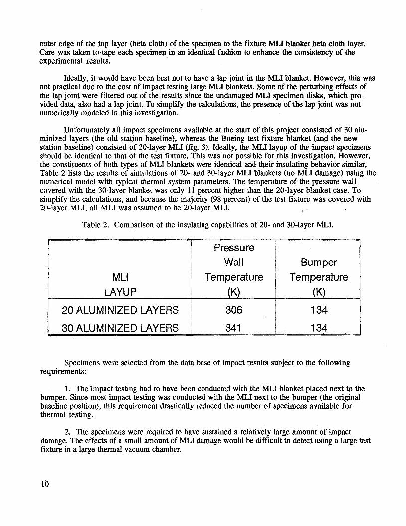
Unfortunately all impact specimens available at the start of this project consisted of 30 alu- minized layers (the old station baseline), whereas the Boeing test fixture blanket (and the new station baseline) consisted of 20-layer MLI (fig. 3). Ideally, the MLI layup of the impact specimens should be identical to that of the test fixture. This was not possible for this investigation. However, the constituents of both types of MLI blankets were identical and their insulating behavior similar. Table 2 lists the results of simulations of 20- and 30-layer MLI blankets (no MLI damage) using the numerical model with typical thermal system parameters. The temperature of the pressure wall covered with the 30-layer blanket was only 11 percent higher than the 20-layer blanket case. To simplify the calculations, and because the majority (98 percent) of the test fixture was covered with 20-layer MLI, all MLI was assumed to be 20-layer MLI.
Table 2. Comparison of the insulating capabilities of 20- and 30-layer MLI.
1
Bumper Temperature M LI
I 20 ALUMINIZED ERS 1 306 134
Specimens were selected from the data base of impact results subject to the following requirements:
1. The impact testing had to have been conducted with the MLI blanket placed next to the bumper. Since most impact testing was conducted with the MLI next to the bumper (the original baseline position), this requirement drastically reduced the number of specimens available for thermal testing.
2. The specimens were required to have sustained a relatively large amount of impact damage. The effects of a small amount of MLI damage would be difficult to detect using a large test fixture in a large thermal vacuum chamber.
10

3. The set of specimens selected was required to have a broad range of impact conditions. Spanning the impact parameter domain was necessary so that the sensitivity of the MLI damage to the impact parameters (projectile diameter and so on) could be determined.
Applying these criteria resulted in the selection of the specimens of table 1.
In the next section, the experimental data obtained from testing in the Sunspot 1 thermal vacuum chamber are discussed.
VI. EXPERIMENTAL RESULTS
The numerical model developed during this investigation is designed to model steady-state conditions. Thus, the thermal testing had to be conducted such that data were taken under steady- state conditions. The procedures used to operate the Sunspot vessel have been described by Hoffman6 and Rule.11 The test plan used was very similar to that developed by Boeing.7 A brief discussion of the test procedure follows.
First, a specimen was carefully taped in place on the MLI blanket of the test fixture. Then, the Sunspot chamber was closed and evacuated to less than 10-5 torr, and the LN2 shrouds were cooled to less than -275 OF. Next, 23.05 W were applied to the pressure wall (through heater H6) and the guard heaters on the test fixture (heaters Hl-H5, H7-Hl0, and H19-H25) were energized to maintain approximately adiabatic conditions (zero temperature difference) between the pressure wall plate and the surrounding, supporting test fixture. The guard heater outputs were adjusted peri- odically during the testing to follow changes in the pressure wall temperatures. After allowing a brief time for stabilization, the thermocouple temperature data for the pressure wall and the bumper were collected approximately every 5 min for about 6 h. This procedure was then repeated for the next specimen.
Funding and time constraints dictated that only 1 day was available for testing each speci- men. This allowed approximately 6 h for the test fixture to come to steady-state conditions. This amount of time proved to be adequate for most of the specimens. In any case, fluctuations in the Sunspot shroud temperatures would prohibit the attainment of perfect steady-state conditions no matter how long the experiment was allowed to run.
The relatively high thermal conductivity of the pressure wall and bumper prevented the devel- opment of large temperature gradients in these components. Thus, local temperature gradients in the vicinity of the impact damage were not large enough to characterize the degradation of the insulating capabilities of the LI. Accordingly, only the temperatures of the thermocouples centered on the MLI impact damage were used to calibrate the numerical model. This involved thermocouple 21 on the pressure wall (fig. 2) and thermocouple 47 on the bumper (fig. 4). The steady-state tempera- tures measured for these thermocouples for each of the specimens is summarized in table 3. The temperature versus time plots associated with the data of table 3 can be obtained from the authors. As shown in table 3, different steady-state temperatures were obtained from essentially identical tests, which indicates that the Sunspot vessel shroud temperatures varied somewhat from test to test.
In the next section, the theory and assumptions associated with the numerical model are discussed.
11

Table 3. Experimentally measured pressure wall and bumper steady-state temperatures.
DATA POINT
NUMBER 1 2 3 4 5 6 7 8 9 10 11 12 13 14
MSFC TEST
NUMBER UNDAMAGED UNDAMAGED
1016 1028 1018 1020 1019 1027 1034 1029 1026 1035 1017 1012
MEASURED PRESSURE WALL STEADY STATE
TEMPERATURE (K) 303.3 306.3 307.8 303.8 300.8 300.9 299.2 300.4 303.6 304.8 298.0 303.9 300.8 306.2
MEASURED BUMPER
STEADY STATE TEMPERATURE (K)
133.8 135.1 134.6 133.9 132.3 133.2 134.9 133.4 134.0
I 133.9 135.1 133.9 134.0 133.9
II.
A numerical model to predi developed during this investigation
C program called SUNS for this program is
behavior of impact-damaged numerical model was impleq
gram is available from the authors. A user s section, the the0 , the results of analyzing the experimental
and assumptions associ- ated with SUNSP data using the SU
The main goal of this project was to develop a microcomputer-based design tool to approxi- mately predict the effects of damage to the ML of S.S. Freedom. To be suitable as a design tool requires that the program be easy to use and that solution times be minimized to rapidly provide feedback for design studies. These requirements dictated that the numerical model be made as simple as possible while still retaining the capability to provide physically reasonable results.
The numerical model was based on the assumption of axial symmetry about the center of the amage. A finite-difference analysis approach was used to discretize the system, where an
y symmetric ring of material can be approximately modeled as a single node as shown in figure her levels of accuracy can be obtained by using more nodes and spacing them closer together.
Thus, only a single, radial line of calculation points (nodes) was required for each layer in the thermal system. The numerical model uses the same number of nodes in each layer. The time required to complete a set of calculations increases greatly as more nodes are used.
12

DISK OF MATERIAL REPRESENTED BY NODE
CENTER OF MLI DAMAGE
Figure 6. Finite difference discretization scheme where an axially symmetric disk of material is represented by a single node.
The computer program is designed to automatically refine the mesh of nodes until further refinement produces no change in the results or until the user specified maximum number of nodes per layer is reached. Each refinement halves the radial spacing between the nodes. The advantage of this refinement process is that a coarse mesh (large node spacing) is used to relatively quickly calculate an accurate set of nodal temperatures and heat fluxes which are then used as initial values for the refined mesh. Accurate initial values for the nodal temperatures and heat fluxes greatly enhance the rate convergence to a solution. An accurate solution can usually be obtained faster using a series of progressively finer meshes than if a single fine mesh is used. Also, the multimesh results provide the user with information on the sensitivity of the calculated results to the node spacing.
The pressure wall, MLI blanket, and bumper were assumed to radially extend out to infinity. The presence of ring frames and stringers was not modeled. These would be difficult and computa- tionally expensive to model since they would be arbitrarily placed which would destroy the radial symmetry. Accurate studies of the effects of the ring frames and stringers would require a very detailed, special-purpose thermal model. Such studies are beyond the scope of the design tool under development in this study. However, the presence of the ring frame and stringers was accounted for indirectly during the thermal model parameter calibration process, as will be discussed in the next section.
As was discussed, it was assumed that all the MLI consisted of the same number of layers, and that no lap joints were present in the MLI. It was assumed that the damage in the MLI con- sisted of a circular hole of the same diameter through all of the MLI layers. Deviations from this
13

assumed ideal hole geometry are provided by an experimentally determined parameter called the “diameter ratio” which is described in the next section. Each layer of the MLI is explicitly modeled with an array of nodes. AI1 aluminized layers are modeled in the same fashion. However, the beta cloth layer and the outer Kapton layer are modeled as a single layer since they are not separated by a Dacron netting spacer. Thus, for the insulation system tested, 22 layers had to be modeled: the pressure wall, 19 aluminized MLI layers, the combined Kapton-beta cloth layer, and the bumper layer. The Sunspot vessel was modeled separately as a single node with one set of effective proper- ties.
The numerical model was designed to model steady-state conditions. Steady state means that the heat flux into each node in the system must equal the heat flux out of that node. Thus, an equation can be written for each node to calculate the nodal temperature such that heat influx will equal heat outflow. The MLI is in a vacuum so the modes of heat transfer are by conduction and radiation. Since radiation Heat transfer is a function of temperature to the fourth power, the nodal heat flux equilibrium equations are nonlinear and must be solved by an iterative process. The thermal equilibrium equations are coupled as well-the temperature of a given node depends on the temperature of adjacent nodes in the same layer as well the nodal temperatures of adjacent layers. This complex pattern of heat flow is schematically illustrated in figure 7.
N+l th LAYER
N-1 th LAYER Figure 7. Schematic drawing of heat flow into and out of a typical node.
14

As adapted from Ozisik,'2 the following equation can be written to describe thermal equilib- rium at a node:
where k is the in-plane thermal conductivity of the layer, t is the thickness of the layer, r is the radial position of the node, T is temperature in the layer, qh is the heat flux into the layer at position r from adjacent layers, qout is the heat flux out of the layer at position r to the adjacent layers, and qi is the net flux into the ith node. Equation (1) basically states that the heat conducted away from a node in the plane of the layer must equal the net influx of heat to that node from adjacent layers.
A standard finite difference approach was used to calculate the temperature derivatives at the ith node:
where A is the radial distance between nodes, Ti is the temperature of the the ith node, and Ti-1 and Ti+l are the temperatures of the nodes on each side of the ith node in the layer. The (i-1)-th node is closer to the origin of the coordinate system than the (i+l)-th node.
Note that the (llr) factor prevents equation (1) from being used to calculate nodal tempera- tures at the origin of the coordinate system (r = 0 at node 1) for the pressure wall and bumper layers. The same problem occurs for the special case where there is no hole in the MLI, and, thus, the first node of each MLI layer is at r = 0. This singularity problem was solved'in conjunction with treating the boundary conditions. For the case of a layer with no hole (node 1 at r = 0) axial symmetry dictates that the in-plane radial heat flux through the origin must be zero. This can be ensured by setting (dT/dr) and (d2Tldr2) equal to zero at node 1. Considering the form of equations (2) and (3), this required setting T1 = T2 = T3 and so the temperatures at nodes 1 and 2 were simply set equal to that of node 3. The same approach was also used for the MLI layers for the case where there was a hole in the MLI, since here there was also no radial flux at node 1 because of the presence of the free edge.
The technique used to treat the boundary conditions at the outer edge of the modeled area will now be discussed. The user of the program specifies the radius of the area to be modeled and the number of nodes, N, per layer. The Nth node would be located on the outer edge of the modeled area. To preserve a type of symmetry in the matrix of governing equations, the computer program automatically adds an (N+l)-th node to each layer. It was assumed that at the Nth node the per- turbing effects of the MLI hole have died out. Thus, the radial heat flux would be negligible and the radial temperature profile uniform at the Nth node of each layer. This boundary can be modeled by setting TN and T N + ~ equal to TN-I. This same boundary condition would apply if the boundary of the
15

area modeled was aligned with the outer edge of the pressure wall plate, the bumper plate, and the MLI blanket. Thus, the inner and outer boundary conditions for every layer were treated in an identi- cal fashion.
Substituting equations ( 2 ) and (3) into equation (1) produces the following equation which describes thermal equilibrium at the ith node of a layer:
Equation (4) can be written in a more compact form as:
where the Cij 0' = 1 to 3) are thermal equilibrium influence coefficients which can be evaluated from equation (4). Equation (5 ) can be expanded in matrix fashion to represent an entire layer of nodal temperatures:
- c 2 2 c23 0 O... 0 0
e31 c32 c33 O. . . 0
0 c41 c 4 2 c43 0 0 0 0 C(N-2)l c(N-2)2 c(N-2)3 0
0 ...o C(N-1)l c(N-1)2 c(N-1)3
T2
T3
7-4
TN-2
TN- 1
TN
f
q2-c2 1 Tl 43
44
q N - 2
4 N - 1
4N-ch9TN+ 1
Equation (6) consists of a tridiagonal system of equations which is very numerically efficient to solve. Note that TI and TN+I are not explicitly solved for, rather they are set equal to T3 and T N - ~ , respectively, of the previous iteration as was mentioned in the boundary condition discussion. An iterative procedure is required to solve equation (6) because the 4i values are complicated nonlinear functions of the nodal temperatures.
The solution procedure consisted of solving equation (6) for the nodal temperatures of the first layer (pressure wall) and then proceeding to the next layer, solving for the nodal temperatures and so forth, until finally solving for the nodal temperatures of the final layer (bumper). This proce- dure is repeated until the nodal temperatures converge with respect to a user defined tolerance.
The calculation of the 4i values will now be discussed. The formulas used to calculate the qi values varied from layer to layer. Accordingly, the method of 4i calculation will be discussed on this basis.
16

A. Pressure Wall Nodal Net Heat Influx Calculations
Every node of the pressure wall was assumed to receive the same magnitude of heat flux from the pressure wall strip heaters since the strip heaters were uniformly distributed over the bottom surface of the pressure wall. The magnitude of this heat influx was determined by dividing the total strip heater input to the pressure wall by the total area of the pressure wall.
The pressure wall radiates heat towards the MLI blanket. This heat flux, qr, is described by the following equation:12
4
q r = E G T ~ 7 (7)
where E is the emissivity of the radiating surface, G is the Stefan-Boltzmann constant [5.6697E-8 W/(m2K4)], and Ti is the temperature of the radiating node. Emissivity values can vary between 0 and 1 depending on the material the surface is made from and the condition of the surface (polished or tarnished and so forth). Emissivity values can vary as a function of time and temperature. In this investigation all emissivities were assumed to be constant.
The pressure wall was exposed to heat flux radiated down from the adjacent MLI layer and from the bumper if a MLI hole is present. Not all of the radiation impinging on thefpressure wall was absorbed. The fraction absorbed is called the absorptivity. To simplify the calculations, the absorp- tivity is commonly assumed to equal the emissivity.12 Radiated energy that is not absorbed is reflected. To preserve conservation of energy, the computer model keeps track of the magnitudes of emitted, absorbed, and reflected radiation. Actually, a portion of the radiation striking the pressure wall from the adjacent MLI layer and from the bumper through the MLI hole is reflected radiation from these layers.
The simplest case of no MLI hole will be considered first. Here, all the nodal temperatures of the MLI layer next to the pressure wall will be identical after equilibrium is attained. Thus, the ther- mal radiation emitted and reflected will be the same for each node in the MLI layer. Also, no thermal energy from the bumper will strike the pressure wall. Accordingly, for this simple case, the compute program uses the thermal radiation (both emitted and reflected) from itQ node of the MLI next to the pressure wall when calculating the heat influx to the ith node of the pressure wall.
The more general case with a hole in the MLI is considerably more complicated. Here, the thermal radiation coming from each node of the MLI layer next to the pressure wall will vary. Also, some of the thermal radiation given off by the bumper will pass through the hole in the MLI and strike the pressure wall plate. The concept of view factors12 was used to treat this problem.
View factors give the fraction of the thermal radiation given off from a surface that will strike another surface of known geometry and position. Consider figure 8 where thermal energy is radiating from circular area A1 to circular area A2. In figure 8, the plane of area A1 is parallel to the plane of area A2. The view factor associated with this geometry, FAI-A~, is given by:12
1+G2+H2 -d( 1 +G2+H2)2 -4G 2 2 H F A l - A 2 =
2G2 7
where G = b/a and H = c/a (fig. 8). Note, for example, that F A ~ - A ~ approaches unity as c (and thus G) approaches infinity as one would expect because for this case area A1 would be radiating into an infinite plane and thus all radiation would be captured.
17

AREA A,
a
AREA A, Figure 8. View factor geometry.
As is illustrated in figure 6, the numerical model developed during the course of this investi- gation is based on the assumption of axial symmetry. Thus, a view factor, Fr, for radiating from ring area to ring area is required here. Fr can be obtained by repeatedly applying equation (8) (fig. 9):
A 1 1 ( F A 1 1-AZl-FA 1 1-A22) -A 12(FA 12-A2 1 -FA 12-A22) Fr = A 1 1 4 1 2
(9)
Thus, Fr specifies the fraction of the energy that is radiated by A A 1 (= A l l - A 1 2 ) that will strike M 2 (= A21-422) .
The total heat influx to the ring corresponding to the ith node of the pressure wall from the adjacent MLI layer was calculated by a summation formed from repeatedly using equation (9) for each node (and thus corresponding ring) of the MLI layer. This is shown schematically in figure 10. The outer boundary of the ring corresponding to the Nth node of the MLI layer was extended out a large distance beyond the user specified radius of modeled area. This was done to be compatible with the assumption that the layers extend out to infinity in all directions.
18

I DIAMETER OF AREA A, , I I ‘I
MLI
DIRECTION OF HEAT FLUX
I DIAMETER OF AREA A,,
I I
Figure 9. Ring-to-ring view factor geometry.
3LE MLI LAYER
EAT INFLUX FROM RINGS OF MLI LAYER TO NODE
OF PRESSURE WALL RING
,
PRESSURE WALL
I
Figure 10. Heat flux from rings of the first MLI layer to a node in a pressure wall ring.
19

The heat flux from the bumper to the pressure wall through the hole in the MLI was treated in two steps. First the ring approach of equation (9) was used to calculate to total heat flux to the MLI hole from each node on the bumper. For this calculation A22 (fig. 9) was set to zero and A21 corre- sponded to the area of the MLI hole. Then, the thermal energy impinging on the MLI hole was allo- cated to the pressure wall node under consideration by using equation (9) again. For this calculation A12 was set to zero and A l l was set equal to the area of the MLI hole. This process is illustrated in figure 11.
MLI HOLE
BUMPER
FLUX FROM
MLI BLANKET
HEAT FLUX FROM MLI OLE TO PRESSURE WALL
PRESS U RE WALL
Figure 11. Schematic drawing illustrating the method of calculating heat flux to the pressure wall from the bumper through the MLI hole.
B. Nodal Net Heat Influx Calculations for MLI Layer Next to Pressure Wall
The MLI layer next to the pressure wall (first MLI layer) can radiate energy to both the pressure wall and the next MLI layer. Thus, the qr for this layer will be twice that given by equation (7).
The pressure wall can subject the nearest MLI layer to both emitted and reflected thermal radiation. This was treated in exactly the same way that MLI heat flux impinging on the pressure wall was treated (reverse of fig. lo), which has been discussed. Note that the MLI layer next to the pressure wall is blocked from receiving radiation from the bumper.
The MLI layer nearest the pressure wall will also be subjected to emitted and reflected radiation from the next MLI layer (second MLI layer). Since the MLI layers are so close to each other, a view factor approach of equation (9) was not used here. The thermal radiation flux from the second MLI layer striking the ith node of the first MLI layer was assumed to equal the thermal radiation flux from the ith node of the second MLI layer.
20

Conduction between the first and second MLI layers was inhibited by the presence of a layer of Dacron netting. The heat flux to the first MLI layer from the second MLI layer through the Dacron netting, q N , was assumed to be of the following form:
where h N is the effective netting heat transfer coefficient (NETCOND), and Ti,l and Ti,2 are the temperatures of the ith node of the first and second MLI layers, respectively. A value for hN was determined by fitting the computer model to the experimental data as will be discussed. It was assumed that the netting heat transfer coefficient was the same for all netting layers.
C. Nodal Net Heat Influx Calculations for a Typical A1 Nzed MLI Layer
Here the net heat influx, qi, to the nodes of the MLI layers between the the fist (next to pressure wall) and last (next to bumper) MLI layers are considered. The qj values for the nodes of these layers are calculated in a similar fashion to what was done for the first MLI layer, except here
LI layers radiating into the MLI layer under consideration. No view factor calcula- tions are required here since the layers are assumed to be close together.. Also, there are two layers of Dacron netting next to each MLI layer, and thus equation (10) will have to be applied twice-once for the layer above and once for the layer below. r
r Layer Next to Bumper
As was noted previously, the last aluminized MLI layer (closest to bumper) and the beta cloth layer are not separated by a layer of Dacron netting (fig. 3). Accordingly, these layers were analyzed as a single layer with the inside surface having the emissivity of an aluminized layer and the outside surface having the emissivity of the beta cloth layer. The thermal conductivity of the layer was assumed to equal the weighted average (on the basis of thickness) of the two layers. For qi calculation purposes this combined layer was treated in exactly the same manner as the first layer except that here the bumper takes the place of the pressure wall.
eat x Ca s for ayer
The net heat influx to the bumper layer was calculated in a very similar manner to that of the pressure wall. The bumper will be subjected to heat i hole just as the pressure wall was from the bumper. , unlike the pressure wall, there were no strip heaters on the bumper. Instead, the bumper interacted with the LN2 shrouds of the Sunspot vessel. For simplicity, the Sunspot shrouds were treated as a single node and average properties were used.
the pressure wall through the
This concludes the discussion of qi calculation for the various layers of the thermal system.
The program uses two types of iterative loops during the solution process. One loop is asso- ciated with solving equation (6), where iterations are necessitated by the nonlinear right hand side, which is a function of temperature. The other iterative loop involves global iterations, which are dis- cussed below. The computer program uses two parameters to control the solver iteration process- the number of solver iterations and the solver relaxation factor. It was found that using two solver iterations was most efficient for solving the systems of equations considered here.
21

The relaxation factor is used to accelerate the rate of convergence of an iterative pr0~ess . l~ It is used to adjust the newly calculated value for a variable based on the value of that variable used at the start of the iteration. For instance, consider the case where a variable had a value of 1 at the start of an iteration and the calculated value at the end of the iteration was 2. If the relaxation factor was 0.5, then the value of the variable that would be used at the start of the next iteration would be 1+(2-1)x0.5 = 1.5. Thus, relaxation factors less than unity correct for overshooting, and those greater than unity correct for undershooting, in the iterative process. As determined by numerical testing, the most effective solver relaxation factor was 0.9.
Nodal temperatures were calculated layer by layer starting with the pressure wall, and finishing with the bumper. A set of calculations covering all layers once was considered one global iteration (as opposed to solver iteration). The computer program uses two factors to control the global iterations-the maximum number of iterations for a given mesh size, and the global relaxation factor.
It typically takes many thousand global iterations until the nodal temperatures converge. After convergence is reached, the program refines the mesh and then starts calculations for the new mesh. If the finest mesh is being used when global convergence occurs, then the program stops. If the maximum allowable number of global iterations (a user input parameter) is used before conver- gence is obtained, then the program refiies the mesh and begins calculations again. If the finest mesh is being used and convergence is not obtained before the maximum allowable number of global iterations has been exhausted, then the program issues a warning and stops.
Fifty global iterations are conducted between each check for convergence. Convergence is assessed by calculating magnitude of the change that occurred in the temperatures of the inside and outside edge nodes of the pressure wall and bumper layers during the 50 global iterations. The change in temperature is divided by the magnitudes of the temperatures to produce a nondimensional relative temperature change. The relative temperature change is compared with a user input conver- gence factor. If the relative temperature change is less than the convergence factor then the calcula- tions were considered to have converged.
The global relaxation factor is similar in nature to the solver relaxation factor. The global relaxation factor is used to adjust the results of a global iteration (based on the results of a previous iteration) to accelerate the rate of convergence. Table 4 illustrates the results of a numerical experi- ment to determine the optimal global relaxation factor. Here, baseline station thermal properties were used, and the solution for a 2.25-in diameter MLI hole was determined starting from the con- verged solution for a 2-in diameter hole. Note that using global relaxation factors greater than 2.01 caused the numerical scheme to diverge. Thus, the recommended value for the global relaxation fac- tor is 2.0. Table 4 also illustrates that using different relaxation factors produced slightly different final results because different solution paths were followed.
Relaxation factors attempt to accelerate convergence by using the values calculated for both the current and the previous iteration. Relaxation factors may not work well during the fiist few iterations since here the solution usually thrashes-especially if the initial values are poor. computer program is set up to gradually apply the relaxation over the some initial number of itera- tions which is specified by the user.
As has been discussed, the computer program has been designed to automatically refine the mesh by halving the distance between the nodes. The idea is to have coarse meshes provide
22

Table 4. Global relaxation factor convergence study.
RELAXATION FACTOR
0.50
1.00
1.50
2.00
2.01
2.02
SOLUTION TIME (SEC)
4249
3400
3046
2833
2833
DIVERGED
RELATIVE PRESSURE WALL SOLUTION TEMPERATURE
TIME ~ (OF)
1.08
1.00
1.00
INFINITY
1.50
1.20
84.50
84.49
84.49
?
84.60
84.53
306.07 0.41
BUMPER TEMPERATL’RE
(OF)
-218.9
-219.0
-219.0
-219.0
-219.0
?
5 9 17 33 65
infinity
I a 2 in diameter to a 2.25 in diamete; MLI hole.
0.2000 0.1 1 1 1 0.0588 0.0303 0.01 54 0
accurate initial values for successively finer meshes. This serves two purposes: the rate of convergence is enhanced and information on the sensitivity of the calculated results to the mesh density is provided. Ideally, the mesh should be refined until there is an acceptably small change in the calculated results.
Table 5 shows typical results of a mesh density study. Here 5, 9, 17, 33, and 65 nodes per layer were successively used in the calculations. The resulting pressure wall temperatures (at ther- mocouple 21) are reported. The MLI had a 1-in diameter hole and typical station baseline thermal
Table 5. Typical results showing the sensitivity of the calculated pressure wall temperature to mesh density.
CALCULATED PRESSURE
WALL TEMPERATURE
306.00 305.62 305.1 3 304.89 304.83
A
_--- Regression Outp
No. of Observations Degrees of Freedom X Coefficient(s)
ERROR WRT , EXTRAPOLATED
305.48 305.1 3 304.94 304.85 0.03 304.74
304.74 0.1 0 0.97 5 3 6.62
23

properties were used. Table 5 also shows interpolated temperature values based on a successful (R2 = 0.97) linear fit through the temperature data using the reciprocal of the number of nodes per layer as the independent parameter. The fitted line can be used to extrapolate the temperature (304.74 K) for the case of an infinite number of nodes per layer, the theoretically exact answer, where the independent parameter is set to zero (= 1/00). The data and fitted line are shown in figure 12. On the basis of this extrapolated temperature, percentage error values for the calculated temperature values were calculated and listed in table 5. Note that even the coarsest mesh had a relatively small error.
Finally, some typical results of pressure wall and bumper temperatures versus MLI hole diameter are shown in figure 13 to provide the reader with an idea of the sensitivity of the thermal system to the MLI hole diameter. Baseline thermal parameter values were used while making these plots.
The next section discusses the process of fitting the numerical model to the experimental data.
I
306.5
E'
3 306
W
W U
5 W a 2
305.5 -I a 3 W LT
2 305 v) W U a EXTRAPOLATED PRESSURE WALL
TEMPERATURE = 304.74 K
304.5 0 0.02 0.04 0.06 0.08 0.1 0.12 0.14 0.16 0.18 0.2
RECIPROCAL OF NO. OF NODES PER LAYER
Figure 12. Plot of pressure wall temperature versus the reciprocal of the number of nodes per layer to show the sensitivity of the solution to the mesh density.
24

(a) PRESSURE WALL
80 f
78 I I I I 1
0 0.5 1 1.5 2 2.5 MU HOLE DIAMETER (IN)
-21 7.8
n -21 8 LL
8 -218.2 -0 Y
-218.4 3 2 -218.6 a W a -218.8 2 W k- -219 U w 2 -219.2 3 m
-21 9.4
-2
Figure 13.
\ 9.6 1 I I I I I
0 0.5 1 1.5 2 2.5 MLI HOLE DIAMETER (IN)
I
Pressure wall and bumper temperatures versus MLI hole diameter calculated by the computer model.
25

VIII. ANALYSIS OF THE EXPERIMENTAL DATA USING THE NUMERICAL MODEL
The results of analyzing the experimental data using the numerical model are discussed in this section. The purpose of the analysis is to show that the numerical model can be made to ade- quately represent the behavior of the thermal system and to empirically fit parameters associated with the thermal system. The end product of analyzing the experimental data is a validated and Cali- brated numerical model that can then be used for making predictions of system behavior.
The input parameters used for the numerical model are listed in table 6, which is an annotated input deck for the computer program. The values of the parameters used were typical handbook values except where noted below. The contents of table 6 will now be discussed.
The MLI hole diameter refers to the approximate diameter of the aluminized layers of the MLI hole. As will be discussed, this actual MLI hole diameter will be adjusted using a parameter called the diameter ratio. The program is also designed to treat the case of no MLI hole as well. The MLI standoff is the average distance between the MLI blanket and the pressure wall. A 5.08-cm (2-in) standoff was assumed while analyzing the experimental data.
During all of the testing associated with this investigation, 23.05 W were applied to the total pressure wall area (4.0645 m2). The estimated pressure wall and bumper temperatures contained in the table 6 are used by the program as initial values in the iterative process if no initial values file is available from a previous analysis. More information on the initial values file is provided in the next section. The temperature conversion factors are used by the program to convert the temperature scale used for calculations (degrees Kelvin) to another scale for ease of reading in the output. The temperature conversion factors shown in table 6 are for converting from degrees Kelvin to degrees Fahrenheit.
r
The number of layers of MLI refers to the number of aluminized layers in the MLI blanket. This actually accounts for the beta cloth layer, since this layer is included with the adjacent MLI layer for calculation purposes, because no Dacron netting spacer was placed between these layers. Twenty MLI layers were modeled in this investigation. Thus, 22 layers were modeled in all--MLI plus pressure wall and bumper.
The test specimen was essentially divided into two equal areas thermally due to the pres- ence of the ring frame. Thus only one half of the pressure wall area was modeled (2.03 m2). The model developed here is based on the assumption of axial symmetry. Thus, the modeled area of 2.03 m2 was treated as an equivalent circular region of the same size. The radius of the area modeled used in the calculations was (2.03/~)0-5 = 0.804 m.
The layer thicknesses for the model were determined from Solomon9 and B~itekant .~ The bumper standoff is the distance that the bumper is separated from the pressure wall.
The effective Sunspot shroud temperature (K) was determined by fitting the computed results to the experimentally measured values. As will be discussed, fitted values varied between 118.3 K and 122.7 K. Solomon9 presented results showing that the measured Sunspot shroud temperatures typically vary between 89 K and 122 K. Thus, the fitted values of the Sunspot shroud temperature seem reasonable.
26

Table 6. Annotated input file for the SUNSPOT computer program.
0.0 > MLI hole d iameter (m) 5.08E-2 > MLI s tandoff (m) 23.05 > to ta l hea t e r input to pressure wall ( W ) 4.0645 > t o t a l p ressure wall area (m 1 295 > est imated pressure wall t e m p e r - a t u r ~ ( K ) 100 -459.67 > t empera tu re conversion f a c t o r number 1 1.8 > t empera tu re conversion f a c t o r number 2 20 > number of layers of MLI (excluding be ta c lo th and dacron ne t t ing) 0.804 > rad ius of area modeled (m) 3.175E-3 > pressure wall thickness (m) 6.35E-6 > average aluminized layer thickness of MLI (m) 5.08E-5 > beta c loth thickness (m) 1.524E-3 > bumper thickness (m) 1.016E-1 > bumper s tandoff (m) 120 > ef fec t ive Sunspot shroud t empera tu re ( K I 130 > pressure wall thermal conductivity (W/mK) 50 > MLI aluminized layer thermal conductivity (W/mK) 1
1.0687 5 > beta c loth thermal conductivity (W/niK) 115 0.06 > pressure wall emissivity 0.06 > MLI aluriiiriized layer emissivity 0 .94 > beta c loth emissivity 0.94 > bumper emissivity outward 0.14 > bumper emissivity inward 0.90 > ef fec t ive Sunspot shroud emissivity 5.6697E-8 > Stefan-Boltzmann cons tan t ( W/m2K4) 1.OE4 > maximum number of global i t e ra t ions f o r a given mesh s ize 2.0 > re laxa t ion f a c t o r f o r global i t e ra t ions 200 > number of global i t e ra t ions before re laxa t ion i s applied fu l ly 1.OE-5 > convergence f a c t o r 2 > maxirrium number of solver iteratioris 0.9 > re laxa t ion f a c t o r f o r solver i t e ra t ions 10 > initial number of nodes in a layer of t h e model 10 > f ina l number of nodes in a layer of t h e model 32 > maximum number of layers in t h e model
2
> es t imated bumper tempera ture ( K )
> ef fec t ive heat t r a n s f e r coeff ic ient of dacron ne t t ing (W/m2K)
> bumper thermal conductivity (W/mK)
27

The effective heat transfer coefficient of the Dacron netting (called NETCOND) was also determined by fitting the computed results to the experimentally measured values. As will be dis- cussed, the fitted value was 1.0687 W/m2 K. An approximate value for NETCOND was developed as follows. Based on a microscopic examination of a sample of the netting, the netting was assumed to consist of a square mesh of 0.2-mm diameter fibers on 3-mm centers. The thermal conductivity of Dacron at the temperatures encountered in the Sunspot chamber was assumed to equal 0.1 W/m K.14 l5 The Dacron netting was also assumed to have uninterrupted contact with the two adjacent MLI layers. Based on these assumptions, the estimated heat transfer coefficient of the Dacron netting was 67 W/m2K. However, the aluminized layers of the MLI tend to crinkle somewhat and the netting is not perfectly flat since it is woven. Thus, far less than perfect contact between the netting and the adjacent MLI layers would be expected. Accordingly, the value of NETCOND obtained from fitting the experimental data to the numerical model, 1.0687 W/m2 K, seems reason- able.
The emissivity values used were all obtained from Solomon.9 The bumper’s two surfaces had different emissivities because the outside surface (farthest from pressure wall) had a special coating (S 13GLO).
Three parameters had to be fitted from the experimental data: the diameter ratio associated with each data point, the effective Sunspot shroud temperature associated with each data point, and the effective heat transfer coefficient of the Dacron netting that was assumed to be the same for all specimens tested. These three parameters will now be discussed.
The diameter ratio is defined as the apparent hole diameter (as determined by running the numerical model to determine the best fit to the experimental data) divided by the measured average diameter of the hole in the aluminized layers. Thus, the diameter ratio is an empirical adjustment (correction) multiplier for the actual (physically measured) hole diameter. It is intended to account for two effects:
1. The diameter of the hole in the beta cloth is somewhat different from that of the aluminized layers.
2. The damage to the aluminized layers of the MLI may extknd a considerable distance back from the apparent edge of the MLI hole. This damage typically takes the form of crinkling? melting, charring, and tearing of the delicate aluminized layers due to the intense heat and shock waves gen- erated by the impact.
It is assumed that the diameter ratio can be correlated to the impact parameters (particle diameter and so forth). The results of a correlation study to fit the calculated diameter ratios to the impact parameters will be discussed presently. The idea is to use the results of this investigation to predict suitable diameter ratios for use in future design studies. The diameter ratio was allowed to vary from 0.6 to 1.4 during the parameter adjustment process. Diameter ratios beyond these bounds were not considered to be physically reasonable.
Precise control of LN2 shroud temperatures was not possible for the large Sunspot vessel. Thus, the shroud temperatures varied somewhat from specimen to specimen, and while a given specimen was being tested. Also, it is not clear how to determine an appropriate single effective
28

shroud temperature, which is required for the computer program, based on the measured tempera- tures of the six shrouds. Hence, the effective Sunspot shroud temperature was considered to be an adjustable parameter in the numerical model of each of the 14 specimens tested.
empirically derived from the experimental data. A single value was used for all layers of every specimen. The magnitude of this parameter depends on the thermal conductivity of the netting material and the fraction of the netting area that actually touches two adjacent MLI layers. Both of these factors are difficult to predict analytically.
The effective heat transfer coefficient of the Dacron netting (called NETCQND) was also
The technique used to fit the parameters to the experimental data will now be discussed. First, data point 1 (undamaged specimen) was used to determine preliminary values for NETCOND and the effective Sunspot shroud temperature. Here, these parameters were adjusted (to five sig- nificant digits) until the calculated pressure wall and bumper temperatures closely matched those measured for this specimen. The resulting values for NETCOND and the effective Sunspot shroud temperature were 1.1249 W/m2 K and 1 19.40 K, respectively.
To adjust the parameters in an effective fashion, pairs of linear functions (first order Taylor expansions) describing how the pressure wall (thermocouple 21) and bumper (thermocouple 47) temperatures varied as a function of the parameters were developed. To increase the accuracy of the Taylor expansions, pairs of functions were developed for each of the aluminized layer hole diameters tested: 1.5, 1.9, 2, 2.1, and 2.2 in (table 1). A pair of functions was also developed for the undamaged specimens that did not include the MLI hole diameter ratio as a parameter. These functions were of the form:
pressure wall: T = ai+aia+aihN+a$y , (11)
bumper: T = bi+bia+bihN+bdy ,
where a; and b; are function coefficients to be fit from calculated results of the numerical model for the ith MLI hole diameter, a is the MLI hole diameter ratio, hN is the NETCOND, and yis the effective Sunspot shroud temperature. Each of the functions of equation (1 1) has four coefficients, thus four linearly independent data points are required to calculate these coefficients.
This was accomplished by calculating the pressure wall and bumper temperatures at a base- line point for each hole diameter (a = 1.00, hN = 1.1249, and y= 119.40) and at three other points where separately: the baseline hole diameter ratio was multiplied by 1.2, the NETCQND magnitude was multiplied by 1.05, and the Sunspot shroud temperature was multiplied by 1.05. A larger multi- plier was used for the hole diameter ratio because the calculated temperatures are less sensitive to this parameter. The four calculation points for each MLI hole diameter are listed in table 7. Only three data points were required for the fitting the functions for the case of no MLI hole since the a parameter was not included in these functions.
The next step involved adjusting the a, hN, and yparameters (based on the Taylor expansion functions equation (1 1)) until the sum of the squared differences between the calculated and meas- ured pressure wall and bumper temperatures of all 14 data points was minimized. This amounted to essentially a least-squares approach to parameter adjustment. As was noted above, the MLI hole diameter ratio and the Sunspot shroud temperatures were allowed to vary from specimen to specimen, but only a single NETCOND parameter was fit for all the data points.
29

Table 7. Sensitivity of calculated temperatures to ML,I hole diameter, Dacron netting heat transfer coefficient, and effective Sunspot shroud temperature.
BASELINE MLI HOLE Dl AM ETE R
0.000 0.000 0.000 3.81 0 3.81 0 3.81 0 3.81 0 4.826 4.826 4.826 4.826 5.080 5.080 5.080 5.080 5.334 5.334 5.334 5.334 5.588 5.588 5.588 5.588
-E!L
NOTES:
- PARAMETER MULTIPLIERS FOR FUNCTION
EXPANSION CALCULATIONS DACRON NETTING SUNSPOT
MLI HOLE HEAT TRANSFER SHROUD DIAMETER COEFFl GI ENT TEMPERATURE
--- 1 .oo 1 .oo
---- 1 .oo 1.05 1 .oo 1 .oo 1 .oo 1.20 1 .oo 1 .oo 1 .oo 1.05 1 .oo 1 .oo 1 .oo 1.05 1 .oo 1 .oo 1 .oo 1.20 1 .oo 1.00 1 .oo 1.05 1 .oo 1 .oo 1 .oo 1.05 1 .oo 1 .oo 1 .oo 1.20 1 .oo 1 .oo 1 .oo 1.05 1 .oo 1 .oo 1 .oo 1.05
CALCULATED
PRESSURE BUMPER
306.41 4 134.705 303.634 134.705 307.666 ~ ;El;: 303.376 302.226 134.126
134.300 300.805 304.583 138.756 301.81 8 134.069 300.1 95 133.842
134.090 299.351 303.002 138.553 30 1 -400 134.01 1 299.660 133.767 298.961 134.034 302.58 1 138.499
1. THE BASELINE DACRON NETI-lNG HEAT TRANSFER COEFFICIENT FOR ALL SETS OF ANALYSES WAS 1.0687 W/(m * 2 K). 2. THE BASELINE SUNSPOT SHROUD TEMPERATURE FOR ALL SETS OF ANALYSES WAS 120.64 K.
30

The parameter fitting procedure just described was repeated using the newly calculated NETCOND parameter and the average of the best fit Sunspot temperatures as baseline parameters to replace the first set of baseline parameters (hn = 1.1249 and y= 119.40). This involved fitting a new set of linear functions, equation (1 1). The least-squares calculations were then repeated and a new NETCOND parameter hn = 1.0687 W/m2 K determined. The average best fit Sunspot tempera- ture from this parameter fitting cycle was y= 120.64 K. The parameter fitting scheme was repeated again and no change in the NETCOND parameter was noted. The parameter fitting process was then considered to have converged.
The calculated temperatures that were used to fit equation (1 1) during the last parameter fitting cycle are listed in table 7. The measured and calculated (per equation (1 1)) temperatures and the best fit parameters derived from the last parameter fitting cycle are shown in table 8.
As can be seen from table 8 and as was discussed, the diameter ratios were not allowed to go outside of the range 0.6 to 1.4. Data points that were constrained by this range (3, 10, 11, and 14) during the least-squares parameter fitting process were considered to be poor quality data points. The poor quality of these data points could have been caused by the specimens not being in a steady-state condition when the final temperature readings were taken or perhaps the guard heaters were not adjusted perfectly such that a significant amount of unaccounted for thermal energy was entering or leaving the system. The poor quality data points were not used when attempting to fit the calculated best fit diameter ratios to the impact parameters as will be discussed. '
Table 8. Thermal test data reduction results.
Data Point
1 2 3 4 5 6 7 8 9 10 1 1 12 13
MSFC Test No.
undamaged undamaged
1016 1028 1018 1 020 1019 1027 1034 1029 1026 1035 1017
14 1012 jest Fit Netcond = 1.0687 v\i P - n " 7 K\
Calc. Pres. Wall
Temp.
305.9 306.5 305.8 303.8 300.8 300.9 299.1 300.4 303.6 304.7 298.3 303.9 300.8 304.5
(K) (K) I (K) 133.8 I 133.0 I 118.3 135.1 134.6 133.9 132.3 133.2 134.9 133.4 134.0 133.9 135.1 133.9 134.0 133.9
1 35.1 133.9 132.3 133.2
133.3 134.0 133.9 135.0 133.8
121.1 121.4 120.0 1 18.3 119.6 122.3 '
119.9 120.2 119.8 122.7 119.9 120.8 120.4
Best Fit Diameter
Ratio
indamaged indamaged 0.600 0.746 1.068 1.090 1.370 1.160 0.769 0.600 1.400 0.693 1.030 0.600
Pressure Wall Regression Results: constant 0 Constant 0 Std Err of Y Est 1.03 Std Err of Y Est 0.29 R Squared 0.85 R Squared 0.88 No. of Observations 14 No. of Observations 14 Degrees of Freedom 13 Degrees of Freedom 13
Std Err of Coef. 0.0009 Std Err of Coef. 0.0006
Bumper Regression Results:
X Coefficient(s) 1 X Coefficient(s) 1
31

Plots of calculated versus measured pressure wall and bumper temperatures are shown in figures 14 and 15, respectively. The straight lines in these plots indicate calculated equals measured. The goodcess of fit parameters associated with fitting the data of figure 14 and 15 to their calculated equals measured lines are shown at the bottom of table 8. R2 values of 0.85 and 0.88 for the pressure wall and bumper data, respectively, indicates that good fits were obtained. Thus, the thermal model predicts the experimentally measured behavior adequately.
308 307
306 305
304
303 302
301
300
299 /
/
I 298 1 297 ! I I I I I I I I I I
297 298 299 300 301 302 303 304 305 306 307 3 Measured Pressure Wall Temperature (K)
18
Figure 14. Calculated versus measured pressure wall temperatures at thermocouple 2 1.
135.5
132 I I I I I I I I Measured Pressure Wall Temperature (K)
132 132.5 133 133.5 134 134.5 135 135.5
Figure 15. Calculated versus measured bumper temperature at thermocopule 47.
32

Some means of determining the appropriatk diameter ratio for a given set of impact parame- ters is required. This was accomplished by fitting an empirical function through the diameter ratio data of table 8 that corresponded to impact damaged specimens that had best fit diameter ratios between 0.6 and 1.4. As was discussed, the data points with best fit diameter ratios outside of this range were considered less reliable. The empirical function for diameter ratio that was derived during the course of this investigation is:
diameter ratio = D [0.1978 V3'466 T2.356D;7*'35 (cos 8)1*694+2.575] , (12)
where D is the diameter of the projectile, V is the velocity of the projectile, Tb is the thickness of the bumper, and 8 is the impact angle (fig. 1). Of course, equation (12) should only be used to predict diameter ratios for impact conditions similar to those of this investigation. Otherwise, a diameter ratio of unity can be used as an approximation. The form of equation (12) was derived from Rule.I6
The predictions of equation (12) are compared with the best fit diameter ratios (of table 8) in table 9 and in figure 16. The line in figure 16 indicates predicted diameter ratio equals calculated diameter ratio. A line was fit through the data of figure 16 which had an R2 value of 0.48 as indicated at the bottom table 9. The lack of good fit between the calculated diameter ratios of table 8 and the
Table 9. Results of correlation study between impact conditions and diameter ratio.
1018 1020 1017 1019 1027 1035 1034
1.068 1.090 I .030 1.370 1.160 0.693 0.769
1.066 1.232 1.047 1.21 1 0.959 0.757 0.705
Recrression Results: I Constant 0 Std Err of Y Est 0.14 R Squared 0.48 No. of Observations 8
X Coefficient(s) 0.9835 Degrees of Freedom 7
lStd Err of Coef. 0.0480 1 33

1.4 I
1.3
-= 1.2 0 la U + t 1.1 i!
Q 0.9
.ca 1 n U
; 0.8
0.7
0.6 1 1.1 1.2 1.3
1
0.6 0.7 0.8 0.9
Figure 16. Predicted versus calculated best-fit diameter ratio.
Thermal Model Best Fit Diameter Ratio
1
.4
predicted diameter ratios from equation (12) is probably mainly due to two sources. There was cer- tainly some scatter in the thermal data and thus some error in the calculated best fit diameter ratios. Also, the assumed functional form of equation (12) is not exact. However, figure 16 shows that the trend of the data has been captured.
In the next section, instructions for using the software are presented.
IX. SOFTWARE USER GUIDE
In this section, instructions for using the SUNSPOT computer program are given. Thus, the reader can readily modify some of the assumptions associated the data reduction presented here, and reanalyze the experimental data. Or the program could be used to analyze new data in the future. The program is written in Microsoft BASIC and can be modified and recompiled using either Microsoft QuickBASIC or Microsoft BASIC Professional Development System 7.
The program is installed by copying all the files from the SUNSPOT program floppy to a new directory in the hard drive of the PC. An Intel 286 or higher CPU with math coprocessor is required. EGA or VGA graphics capability is necessary if the program is to be run in graphics mode. The following files are present on the floppy disk:
SUNSPOT.BAS > source code file SUNSPOT.EXE > executable file SUNSPOT.DAT > typical file of input parameters SUNSPOT.0UT > typical output file SUNSPOT.INI > typical initial values file
34

The last three files can be given any valid DOS filenames. The format of the input parameters file was shown in table 6. Of course, the comments of table 6 should not be included in an input file. The output file contains an echo of all of input parameters, as well as calculated pressure wall and bumper temperatures at key thermocouple locations for each mesh density used. Finally, the pres- sure wall and bumper temperatures associated with the final mesh used are listed at the end of the output file. Two output file examples are presented in tables 10 (no MLI hole) and 11 (0.0762 m MLI hole diameter).
Calculations are conducted relatively quickly for the case of no MLI hole since view factor summations are not required. However, calculations performed with a MLI hole can progress very slowly especially if many nodes and a small convergence factor are used in order to produce very accurate final answers. One way to speed up the calculations is to provide an accurate set of initial nodal temperatures and heat fluxes. The initial values file is intended for this purpose. When the program is started, the user is prompted for an initial values file filename. If this file exists, and if it contains results from a previous run that had the same number of nodes and layers as the initial mesh of the current run, then the nodal temperatures and heat fluxes contained in the initial values file are used as initial values for the current run. If the initial values file does not exist (no previous run data available), or if the initial values file contains results for a mesh with a different number of nodes or layers, then the program will derive its initial values from the estimated pressure wall and bumper temperatures given in the input parameters file. 1
When the program attains convergence for the initial mesh used, it overwrites the contents of the initial values file with the current nodal temperatures and heat fluxes. Thus, a copy of an existing initial values file should be made if the user does not wish that an old set of initial values be over- written. In fact, it is recommended that a catalogue of initial values files be maintained that span the domain of thermal parameters of interest. The user can then make a copy of the initial values file that most closely matches the current set of thermal conditions of interest and use this file as the initial values file of the current run. In this way run times can be minimized.
The calculations can be safely stopped at any stage by pressing the F1 function key. Pressing the F1 function key will cause an initial values file to be written out with the nodal temperatures and heat fluxes of the current mesh. Thus, calculations can be restarted where they were halted using this initial values file. When restarting, the user should insure that the ihitial number of nodes per layer specified in the input parameters file matches the number of nodes per layer that was being used when the F1 function key was pressed.
The SUNSPOT program can be run in a graphics or text mode. In the graphics mode, color coded graphs of temperature, relative convergence, and energy emitted from the bumper are displayed on the computer screen as a function of iteration number to help the user monitor the calculations (fig. 17). Pressure wall, MLI (middle MLI layer), and bumper temperatures (all at node 3 of their respective layers) are shown as graphs. These temperatures should reach constant values, and thus the graphs become horizontal, as steady-state conditions are reached. The graph for the energy emitted by the bumper should also become horizontal as steady-state conditions are approached. The relative convergence graph shows the current level of convergence (calculated every 50 iterations) divided by convergence factor specified by the user in the input parameters file. Thus, convergence is reached (for a given mesh density) when the relative convergence is less than or equal to unity. The scales of the graphed items are adjusted automatically to keep all traces from going off-scale.
35

Table 10. Typical output file from SUNSPOT computer program for the case of no MLI hole.
36
MLI hole diameter: ML.1 stand off: Pressure wall heat input: Pressure wall area: Estimated pressure wall temperature: Estimated bumper temperature: Temperature conversion factor one: Tempera twe conversion factor two: Number of MLI layers: Radius of area modeled: Pressure wall thickness: MLI layer thickness: Beta cloth thickness: Bumper thickness: Bumper s tand off Sunspot wall temperature: Thermal conductivity of pressure wall: Thermal conductivity of W-l: Heat t r ans fe r coefficient of Dacron Netting: Thermal conductivity of beta cloth: Thermal conductivity of the bumper: Emissivity of pressure wall: Emissivity of MLI: Emissivity of be ta cloth: Emissivity of ou te r surface of bumper: Emissivity of inner surface of bumper:
0 .0503 23-05 4.0645 295 100
-459.67 1.3
20 .504 .003175
.0000063!5
.oooosoa .001524 -1016
120 130 50 1.0687
5 . 115 .06 -06 -94 .94 -14
Emissivity of inner surface of Sunspot chamber: Stefan-Boltzmann constant: .000000056691 Maximum number of i terations f o r each mesh: Successive Over Relaxation Factor: 2 Relaxation Delay: 200 Convergence Factor: .ooM)1 Maximum Solver Iterations: 2 Solver Relaxation Factor: .9 Initial Number of Nodes: 10 Maximum Number of Nodes: 10 Maximum Number of layers in model: 32 ~ ~ ~ ~ o ~ a o ~ s ~ ~ ~ ~ ~ ~ ~ o ~ o ~ w o o o m a o ~ a o ~ ~ ~ ~ a o ~ ~ ~ w ~ ~ ~ ~ ~ o ~ ~ ~ ~ ~ ~ ~ ~ ~ ~ ~ ~ ~ a ~ n o m ~ ~ w ~ o ~ ~ ~
No. of Mesh Points: 10
PRESSURE w w :
.9
10000
IThermocouple 211
IhU, M2, M3. M 4 l
(20. 221
9.166D+O1
9.166D+01
9.166D+01 BUMPER.
[Thermocouple 471
IM9, M10. .MU, MU1
INS. M6. MI, M81
-2.180D+02
-2.180D+02
-2.180D42
Final Nodal Temperatures: ~ ~ ~ ~ ~ ~ ~ ~ ~ ~ ~ ~ ~ o ~ ~ ~ ~ o ~ n o o o o ~ o o ~ ~ ~ o o ~ o ~ ~ ~ m n ~ ~ a ~ ~ o ~ ~ ~ ~ ~ o ~ ~ ~ o o ~ ~ . i ~ ~ ~ ~ a ~ ~
Node No. Pressure W a l l Bumper 1 9.166M1 -2.180D+02 2 9.166W1 -2.180D+02 3 9.166D+01 -2.180D+02 4 9.166W1 -2.180D+02 5 9.166D+01 -2.1808+02 6 9.166W1 -2.180W2 7 9.166M1 -2.180D+02 8 9.166W1 -2.180M2 9 9.166M1 -2.180W2 10 9.166D41 -2.180M2
a o ~ ~ m o a a o ~ ~ m m ~ ~ a ~ a o ~ ~ m o o ~ m a ~ a - . . o ~ o a o o e ~ ~ ~ ~ ~ . ~ ~ ~ ~ ~ ~ ~ ~ ~ m ~ ~ m ~ ~ e o o o o w w ~ ~ o m o ~

Table 11. Typical output file from SUNSPOT computer program for the case of a 3-in diameter MLI hole.
MLI hole diameter: MLI stand off: Pressure wall hea t input: Pressure wall area: Estimated pressure wall temperature: Estimated bumper temperature: Temperature conversion fac tor one: Temperature conversion f a c t o r two: Number of MLI layers: Radius of area modeled: Pressure wall thickness: MLI layer thickness: Beta cloth thickness: Bumper thickness: Bumper s tand off : Sunspot wall temperature: Thermal conductivity of pressure wall: Thermal conductivity of MLI: Heat t r a n s f e r coefficient of Dacron Netting: Thermal conductivity of be ta cloth: Thermal conductivity of t h e bumper: Emissivity of pressure wall: Emissivity of MLI: Emissivity of be ta cloth: Emissivity of ou ter sur face of bumper: Emissivity of inner sur face of bumper: .
.0762 .0508 23.05 4.0655 295 100
-459.67 1.8
20 .804 .003175 .0oO00635 .0000508 .001524 .1016
120 130 50 1.0687 5 1 I5 .06 .06 .94 .94 .14
Emissivity of inner su r face of Sunspot chamber: .9 Stefan-Boltzmann constant: .000000056697 Maximum number of i terat ions for each mesh: 10000 Successive Over Relaxation Factor: 2 Relaxation Delay: 200 Convergence Factor: .00001 hlaximurn Solver Iterations: 2 Solver Relaxation Factor: .9 Initial Number of Nodes: 10 h4aximum Number of Nodes: 10 Maximum Number of layers in model: 32 .s*se.moo-w..o.o....oossoosoo.ooooosmas**soos6a*.~~.o~so~oo~omss~aso~=s~*~*o-o
No. of Mesh Points: 10
PRESSURE WALL: [Thermocouple 211
7.951D+Oi [bll, M2, M3, M41
7.951D+01 [20* 221
7.950D+01 BUSIPER:
-2.106D+02
-2.106D+02
-2.196D+02 s t * a * ~ ~ i l l o s e t o o ( . 9 s ~ 9 ~ 9 a s ~ s s s 9 s o s s s o s a a o s s s o o 9 a ~ a ~ ~ ~ s ~ o ~ s o ~ ~ o s o o ~ o o ~ s ~ ~ o o ~ o s o o
[Thermocouple 471
Ihl9, M10, MU. MlZl
Ih15. M6, M7, M81
Final Nodal Temperatures: Node No. Pressure Wall Bumper
1 7.9511)+01 -2.196Dt02 2 7.951D+01 -2.196D+02 3 7.951D+01 -2.196D+02 4 7.954D+01 -2.196D+02 5 7.958D+Ol -2.196D+02 6 7.9618+01 -2.196D+O2 7 7.963D+Ol -2.196D+02 8 7.965D+01 -2.196Dt02 9 7.965D+O1 -2.196D+02
10 7.9650+01 -2.196DL02 o6~~~~~~~~i~~~~oeoe~.~..................~so~~om~om~~s~~ssg~os~~o~aoe~e8~mm~~~~
37

Ressure Wul Temperature +-- Bumper Energy :
22.171
R e l . Convergence: z .7ze~+ee
No. of Iterations:
84.9218 BUMPER : I
C Thermoeoup le 471 -218.8748
-218.8735 C M S r Ml6r M l l r M12
EMS, M6, Mi', M81
t -218.8742 Bumper Temperature No. Mesh Pts.= 18
Figure 17. Computer screen shown while the SUNSPOT program iterates.
well as other pertinent information. When the calculations have been completed, a color contour plot of pressure wall temperatures is shown on the screen as well as the execution time and a message indicating whether convergence was reached before the user input number of global iterations expired on the final mesh used.
1
Numerical values for all graphed items are given on the right side of the screen (fig. 17) as
The text mode option was provided primarily to allow the SUNSPOT program to run in the background while using Microsoft Windows multitasking software. This allows the user to perform other noncomputationally intensive tasks (word processing, etc.) while at the same time running the SUNSPOT program.Also, multiple runs of the SUNSPOT program (with different thermal parame- ters) can be run at same time using Microsoft Windows. The author successfully ran four SUNSPOT runs simultaneously. In the text mode, only the information shown on the right side of figure 17 is displayed on the screen.
X. CONCLUSIONS AND RECOMMENDATIONS
Listed below are conclusions and recommendations developed during the course of this study.
A. Conclusions
e The damaged MLI specimens were created (impacted) and thermally tested under as real- istic conditions (with respect to the space station) as were possible under the prevailing time and budget constraints.
e The goal of realistic testing conditions prevented some of the thermal system parameters from being tightly controlled which produced some scatter in the measured data that is illustrated by the off-diagonal points in figures 14, 15, and 16. The scatter is most likely due to the difficulty in maintaining steady-state conditions and enforcing the insulated boundary conditions.
38

* The behavior of the thermal test fixture and specimens was adequately represented by the axially symmetric numerical model that was developed during the course of this investigation.
* The proposed parameter, diameter ratio, provides a convenient and practical means of link- ing nominal measures of impact damage to the impact parameters.
B. Recommendations
If more consistent data is desired, then a new test fixture should be developed to provide a means of more tightly controlling or simplifying the thermal parameters associated with the test fixture. One possible test fixture would model the pressure wall, the MLI blanket and the bumper in the form of 2.5-m diameter disks that would be suspended edgewise from the roof of the Sunspot vessel. Low thermal conductivity materials would be used for the suspenders. The impact damage would be placed at the center of the MLI disk. Small, low thermal conductivity spacers could be placed periodically around the edges of the disks to maintain a uniform separation between the disks. The pressure wall disk would be heated with a uniform array of strip heaters. This configuration would eliminate the sag problem, and guard heaters would not be required.
* A catalogue of initial values files that span the domain of thermal parameters of interest should be maintained. Run times can be minimized by selecting the initial values file that is most compatible with the current thermal parameters of interest.
39

REFERENCES
1. Kessler, D.J.: “Predicting Debris.” Aerospace America, June 1988, pp. 22-23.
2. Whipple, E.L.: “Meteorites and Space Travel.” Astronomical Journal, vol. 52, 1947, p. 137.
3.
4.
5.
6.
7.
8.
9.
10.
11.
14.
15.
Taylor, R. A.: “A Space Debris Simulation Facility for Spacecraft Materials Evaluation.” SAMPE Quarterly, vol. 18, February 1987, pp. 28-34.
Schonberg, W.P., Bean, A.J., and Darzi, K.: “Hypervelocity Impact Physics.” University of Alabama in Huntsville, Final Report for NASA Contract No. NASS-36955D.O. 16, 1990.
Kesseler, D.J., Reynolds, R.C., and Anz-Meador, P.D.: “Orbital Debris Environment for Spacecraft Designed to Operate in Low-Earth Orbit.” NASA Technical Memorandum 100471, 1989.
Hoffman, R.J.: “Facility Operating Procedure for Sunspot 1 Thermal Vacuum Chamber.” NASA Document ETGFOP-425, rev. C, 1988.
Buitekant, A.: “PTCS Initial ThermWacuum Development Test, Phases I and 11.” Boeing Document No. D683-10491-1,1990.
I
Jorgensen, A.: “Initial PTCS Pressure Shell Wall Thermal Vacuum Development Test.” Boeing Document No. D683-10422-1,1990.
Solomon, M.: “Passive Thermal Control System (PTCS) Development Test Analysis Report.” Boeing Document No. 2-H8T4-RSB-07 1/90,1990.
Till, W .A.: “Space Telescope On-Orbit Maintenance Mission Process Specifications for MLI Blankets.” Marshall Space Flight Center Specification 1312A, 1988.
Rule, W.K.: “Plan for Testing Hypervelocity Impact Damaged k I in the NASNMSFC Sunspot 1 Thermal Vacuum Chamber Using the Boeing PTCS Development Test Fixture.” Department of Engineering Mechanics, The University of Alabama in Tuscaloosa, 1990.
Ozisik, M.N.: “Heat Transfer a Basic Approach.” McGraw-Hill Book Company, New York, 1985, pp. 1-14,23-37, and 593-642.
Torrance, K.E.: “Numerical Methods in Heat Transfer.” Handbook of Fundamentals; Rohsenow, W.M., Hartnett, J.P., and Ganic, E.N., ed Company, 1985, pp. 5-15-5-16.
Steere, R.C.: “Thermal Properties of Thin-Film Polymers by Transient Heating.” J. of Applied Physics, vol. 37, No. 9, 1966, pp 3338-3344.
Assfalg, A,: “Study of Thermal Conductivity and Specific Heat of Amorphous and Partially Crystalline Poly(ethy1ene terephthalate) in Relation to Its Structure.” J. Phys. Chem. Solids, V O ~ . 36,1975, pp. 1389-1396.
40

16. Rule, W.K.: “MLIBlast-A Program to Empirically Predict Hypervelocity Impact Damage to the Space Station.” NASA contractor report No. CR-184153, 1991, pp. 35-37.
I
41

APPROVAL
SUNSPOT-A PROGRAM TO MODEL THE BEHAVIOR OF HYPERVELOCITY IMPACT DAMAGED MULTILAYER INSULATION IN THE SUNSPOT THERMAL
VACUUM CHAMBER OF MARSHALL SPACE FLIGHT CENTER
By W.K. Rule and K.B. Hayashida
The information in this report has been reviewed for technical content. Review of any information concerning Department of Defense or nuclear energy activities or programs has been made by the MSFC Security Classification Officer. This report, in its entirety, has been determined to be unclassified.
r
J.C. B d f k Director, Structures and Dynamics Laboratory
* U. S. G O V E R N M E N T PRINTING OFFICE 1992 - 631-060/60051
42

SUNSPOT-A Program to Model the Behavior of Hypervelocity Impact Damaged Multilayer Insulation in the Sunspot Thermal V- nf -ht renter
8. AUTHOR(S)
W.K. Rule* and K.B. Hayashida
. PERFORMING ORGANIZATION NAME(S) AND ADDRESS(ES) 8. PERFORMING ORGANIZATION REPORT NUMBER
George C. Marshall Space Flight Center Marshall Space Flight Center, Alabama 358 12
I
I. SPONSORING /MONITORING AGENCY NAME(S) AND ADDRESS(ES) 10. SPONSORING / MONITORING AGENCY REPORT NUMBER
National Aeronautics and Space Administration Washington, DC 20546 NASA TM-103570
I
. 1. SUPPLEMENTARY NOTES Prepared by Structures and Dynamics Laboratory, Science and Engineering Directorate.
Unclassified-Unlimited
I
13. ABSTRACT (Maximum 200 words)
This report describes the development of a computer program to predict the degradation of the insulating capabilities ofthe multilayer insulation (MLI) blanket of Space Station Freedom due to a hypervelocity impact with a space debris particle. \A finite difference scheme is used for the calculations. The computer program was written in Microsoft BASIC. This report also describes a test program that was undertaken to validate the numerical model. Twelve MLI specimens were impacted at hypervelocities with simulated debris particles using a light gas gun at Marshall Space Flight Center. The impact-damaged MLI specimens were then tested for insulating capability in the space environment of the Sunspot thermal vacuum chamber at MSFC. Two undamaged MLI specimens were also tested for comparison with the test results of the damaged specimens. The numerical model was found to adequately predict the behavior of the MLI specimem in the Sunspot chamber. A parameter, called diameter ratio, was developed to relate the nominal MLI impact damage to the apparent (for thermal analysis purposes) impact
ISN 7540-01 -280-5500 Standard Form 298 (Rev 2-89) Prescribed by ANSI Std 239-18 298-102