a.s. jensen & l. wiesenfeld, organizers january 4, 2006
TRANSCRIPT

Critical stability IVProceedings of the Workshop held at Dresden, October
2005
A.S. Jensen & L. Wiesenfeld, organizers
January 4, 2006
Proceedings Edited by A.S. Jensen, J.-M. Richard and L. Wiesenfled
1

Table of contents
Preface 1Frederico 3Kievsky 9Grießhammer 13Fedorov 20Richard 24Greene 30Hiyama 36Barnea 43Miller 49Elander 54Motovilov 60Peeters 66Duclos 70Brummelhuis 76Simonovic 81Brack 87Ostrovsky 94Koon 102Gabern 108Komatsuzaki 114Delos 121Hinde 127Lepetit 132Meremianin 138Kolganova 142Hussein 146Hogreve
2
Few-Body Systems 0, 1–2 (2006) Few-Body
Systemsc© by Springer-Verlag 2006
Printed in Austria
Preface
A.S. Jensen1∗, J.-M. Richard2∗∗, L. Wiesenfeld3∗∗∗
1 Department of Physics and Astronomy, University of Aarhus, 8000 Aarhus C, Denmark,2 Laboratoire de Physique Subatomique et Cosmologie, Universite Joseph Fourier–CNRS-IN2P3,
53, avenue des Martyrs, 38026 Grenoble, France,3 Laboratoire d’Astrophysique de l’Observatoire de Grenoble, Universite Joseph Fourier–CNRS, BP 53,
38041 Grenoble, France
The fourth international and interdisciplinary workshop
Critical stability of few-body quantum systems
was held at the Max-Planck Institute for the Physics of Complex Systems in Dresdenfrom October 16 to 22, 2005. As for the previous workshops, at Trento in 1997 and 2003,and Les Houches in 2001, the main motivation was to discuss questions that are sharedby specialists of different fields, and are formulated, tentatively solved and further de-veloped using slightly different methods and languages. This interdisciplinary charac-ter, ranging from mathematical physics to quantum chemistry, via molecular, atomic,nuclear and hadron physics, was an essential ingredient of these workshops, and linkedwith the foundation of few-body physics. The present meeting increased slightly theemphasis on atomic and molecular physics and also on mathematical-statistical physicsin the area of condensed matter. The following subjects were proposed in the call forabstracts and invitations:
1. Weakly Coulomb or gravitational-bound few-body states.2. Weakly short-range-interaction bound few-body states.3. Continuum structure and few-body decay properties.4. Dynamical few-body problems near instability.5. Correlation in boson-fermion and mixed condensates6. Few-body correlation within many-body systems.7. Exotic structures: Efimov, tango, Borromean and halo states.8. Lower-dimensional systems.9. Semi-classical methods.
We had 50 participants from 19 countries, mostly from Europe and North Americabut also from Japan and Brazil. The number was limited to optimize the interactionamong the participants.∗[email protected]∗∗[email protected]∗∗∗[email protected]

2 Preface
We want to thank the Max-Planck-Institute for the generous financial support, theexcellent organization, and the smooth and efficient running of the workshop. In par-ticular we want to thank Jan-Michael Rost for his continuous support for this projectand Mandy Lochar for taking care of all the logistics. In addition, we are greatful forthe support of Few-Body Systems and its Editor in Chief B. Bakker for hosting the pro-ceedings, thus ensuring a rapid and widespread diffusion. Last but not least, we wantto thank the participants for the lively discussions after the talks and during the breaks,all in the genuine interdisciplinary spirit which is now the tradition of this series. Somemore details about the workshop along with pictures of the participants can be seen onhttp://www.mpipks-dresden.mpg.de/∼crit05

Few-Body Systems 0, 3–8 (2006) Few-Body
Systemsc© by Springer-Verlag 2006
Printed in Austria
Structure of exotic three-body systems∗
T. Frederico1∗∗, M.T. Yamashita2, A. Delfino3, Lauro Tomio4
1Departamento de Fısica, Instituto Tecnologico de Aeronautica, Centro Tecnico Aeroespacial,12.228-900 Sao Jose dos Campos, Brasil.2Unidade Diferenciada de Itapeva, Universidade Estadual Paulista, 18.409-010 Itapeva, Brasil.3 Instituto de Fısica, Universidade Federal Fluminense, 24.210-900 Niteroi, Brasil.4Instituto de Fısica Teorica, Universidade Estadual Paulista, 01405-900 Sao Paulo, Brasil
Abstract. The classification of large halos formed by two identical particlesand a core is systematically addressed according to interparticle distances.The root-mean-square distances between the constituents are described byuniversal scaling functions obtained from a renormalized zero-range model.Applications for halo nuclei, 11Li and 14Be, and for atomic 4He3 are brieflydiscussed. The generalization to four-body systems is proposed.
1 Introduction
The properties of large three-body systems present universal behavior as theThomas-Efimov limit is approached [1]. In this situation the sizes of the twoand three body systems are much larger than the interaction range and the wavefunction almost everywhere is an eigenstate of the free Hamiltonian. Much of thephysics of these systems can be studied using a zero-range interaction effectivein s-wave. No scale is involved in this drastic situation and the momentum spaceFaddeev equations are scale invariant for vanishing two and three-body energies.The scale invariance is broken by finite values of two-body scattering lengths andthree-body binding energy, which are the scales of the corresponding three-bodysystems [2]. Dimensionless ratios of three-body observables are then expressedby scaling functions which depends only on ratios of two (bound or virtual) andthree-body energies [3]. The scaling functions can be obtained from the solutionof regularized Faddeev equations.
The sizes of halo three-body systems (where two particles are identical) arefunctions of few physical scales. A classification scheme for these systems [4, 5, 6]ordered by their sizes is reviewed. For a given three-body binding energy the
∗Article based on the presentation by T. Frederico at the Fourth Workshop on the Dynamicsand Structure of Critically Stable Quantum Few-Body Systems, MPIPKS, Dresden, Germany,2005. Received November 10, 2005
∗∗E-mail address: [email protected]

4 Structure of exotic three-body systems
most compact system is the Borromean (single pairs are unbound) while theall-bound (all single pairs form bound states) is the largest one. The neutron-neutron mean square radius in examples of Borromean halo nuclei which areknown experimentally [7] are briefly discussed. The extension of these ideas tofour-body systems is proposed.
2 Scale invariance in three-boson systems
The collapse of a three-boson system when the two-body interaction range goesto zero (Thomas effect, see [1]) demands one new physical scale to stabilizesthe three-boson binding energy (E3). The regulated trimer bound state integralequation in units of ~ = m = 1 (m is the boson mass) is written as
f(q) = 2πτ(E3 −34q2)
∫ ∞
0k2dk f(k)
∫ 1
−1dz
[G0(E3)−G0(−µ2
(3))], (1)
where G−10 (E) = E − q2 − k2 − qkz, and the renormalized two-boson scattering
amplitude is τ−1(x) = 2π2[a−1 −
√−x
]. Without regularization, Eq. (1) is the
Skorniakov and Ter-Martirosian (SKTM) equation derived long ago [8] whichis scale invariant when the scattering length |a| tends to infinity and E3 = 0.The second term in Eq. (1) brings the physical scale, µ(3), to the three-bosonsystem [2] avoiding the Thomas collapse. The equivalence of Thomas and Efimoveffects is seen in units of µ(3) = 1, which means |a|µ(3) →∞ either for |a| → ∞(Efimov limit) or for µ(3) →∞ (Thomas limit).
The sensitivity of three-boson S-wave observables to the short-range partof the interaction in weakly bound systems is parameterized through the valueof the trimer binding energy which corresponds to the scale µ(3). Three-bosonS-wave observables are strongly correlated to the trimer energy in a generaluniversal form [3, 9]:
O3(E,E3, a) = |E3|ηF3
(E/E3, a
√|E3|
), (2)
where O3 can represent a scattering amplitude at an energy E or an excitedtrimer energy (the dependence on E does not appear in this case). The expo-nent η gives the correct dimension to O3. Eq. (1) is renormalization group (RG)invariant with its kernel being a solution of a Callan-Symanzik differential equa-tion as function of a sliding µ(3). In that way E3 and three-body observablesare independent of the subtraction point (see ref. [9] for a discussion of the RGinvariance in three-body systems).
3 Classification of three-body halos and universal scalings
The sizes of halo three-body systems (with two identical particles (α) and adistinct one (β)) are functions of few physical scales. A classification scheme forthese systems as Borromean (single pairs are unbound), Tango (only the αα pairform a bound state), Samba (only the αβ pair is bound) and all-bound (all singlepairs form bound states), ordered by their sizes is discussed below.

T. Frederico, M.T. Yamashita, A. Delfino, Lauro Tomio 5
The typical lengths of the three-body halo systems are given by scaling func-tions for the mean-square separation distances written according to Eq.(2). Thescaling functions for these radii are:√
〈r2αγ〉|E3| = Rnγ
(±
√Eαα/E3,±
√Eαβ/E3, A
), (3)√
〈r2γ〉|E3| = Rcm
γ
(±
√Eαα/E3,±
√Eαβ/E3, A
), (4)
where 〈r2αγ〉 and 〈r2
γ〉 are, respectively, the mean square relative and center ofmass distances. The mass ratio is A = mβ/mα and γ is α or β. The + or - signsrepresent bound or virtual two-body subsystems, respectively. Eαα and Eαβ arethe αα and αβ two-body energies.
For a given energy E3 and identical particles, the effective interaction inEq. (1) has a weaker strength for a < 0 (virtual two-body system) than for a > 0(bound two-body system). Therefore, for a Borromean trimer Eq. (1) should havea larger value of µ3 than the corresponding one for an all-bound system, in orderto keep the binding fixed with a weaker interaction. The spectator function, f(q),extends to large momentum for a Borromean system. The trimer wave functionfor zero total angular momentum is
Ψ(q, p) =f(|q|) + f(|p + 1
2q|) + f(|p− 12q|)
E3 − 34q2 − p2
, (5)
which implies in a more compact spatial configuration for a Borromean trimerin comparison to the all-bound one. The Jacobi relative momenta are p for thepair and q for the spectator particle. In terms of the scaling functions the radiicome as,
Rαα
(−
√Eαα/E3
)< Rαα
(√Eαα/E3
), (6)
and the separation distances obeys√〈r2
αα〉|E3|B <√〈r2
αα〉|E3|A, where thelabels B and A correspond to Borromean and All-bound systems, respectively.For the same reasons that led to Eq. (6), it is also valid that
√〈r2
α〉|E3|B <√〈r2
α〉|E3|A. The zero-range model applied to atomic 4He3 provides a qualitativeunderstanding of the radii results of realistic calculations for the ground andexcited states [10] with an estimation of
√〈r2
αα〉 = C√
~2/[mα(|E3 − Eαα|)] with0.6 < C < 1 [6]. Also the excited trimer state energy of 4He3, E∗3 , has a scalingbehavior written as√
|E∗3 − Eαα| =√|E3| E
(±
√Eαα/E3
), (7)
which is consistent with results from realistic calculations (see [3, 9] andreferences therein). The threshold for the appearance of an excited Efimovtrimer state from the second energy sheet is |E3| = 6.9/a2 [9, 11] in units of(~ = mα = 1). The scaling behavior was extended to the complex energy planeand for three-boson Borromean systems, the excited Efimov state turns into aresonance when the virtual two-boson virtual state energy is decreased [12].

6 Structure of exotic three-body systems
The generalization of the reasonings leading to Eq. (6) to the ααβ systemgives the qualitative classification of the different three-body systems in respectto sizes. The effective interaction is weaker when a pair has a virtual state thanwhen the pair is bound, and the three-body system has to shrink to keep thebinding energy unchanged if a pair which is bound turns to be virtual. Thereforeit is reasonable to expect that
Rαγ
(−
√Eαα/E3,−
√Eαβ/E3, A
)< Rαγ
(√Eαα/E3,−
√Eαβ/E3, A
)< Rαγ
(−
√Eαα/E3,
√Eαβ/E3, A
)< Rαγ
(√Eαα/E3,
√Eαβ/E3, A
), (8)
which was checked numerically [6]. An analogous relation is valid for Rcmγ . The
dimensionless products (we are using units of ~ = mα = 1)√〈r2
αβ〉|E3| and√〈r2
αα〉|E3| increase from Borromean, Tango, Samba and to All-Bound configu-rations, systematizing the classification scheme proposed in Ref. [5] for weaklybound three-body systems.
A three-body model applied to light exotic nuclei [6] compares qualitativelywell with the existent experimental data for the neutron-neutron separation dis-tance in the neutron-halo of 11Li and 14Be [7]. Therefore, the neutrons of thehalo have a large probability to be found outside the interaction range and thelow-energy properties of the halo are, to a large extend, universal as long as fewphysical input scales are fixed in the model. An insight into the structure of halonuclei can be found even considering the limitations of the model. The finite sizeof the core and consequently the antisymmetrization of the total nuclear wavefunction, are both missing in this simplified description. However, in exampleswhere the neutrons in the halo tend to be more and more weakly bound withvirtual or bound subsystems near the scattering threshold, the scaling relationsapply for the halo properties, as the above limitations are less important.
4 Classification of four-body halos and universal scalings
The four-boson system has two Faddeev-Yakubovsky (FY) independent ampli-tudes and within a zero-range model, they are reduced to spectator amplitudesdepending on two Jacobi momenta. The two spectator FY reduced amplitudessatisfy a coupled set of integral equations generalizing the SKTM equation forthree bosons. The set of coupled integral equations needs regularization, and onerecognizes that the resolvent of the immersed three-boson subsystem carries thescale µ(3). Other terms are present and require regularization. We introduce ascale µ(4) such that the four-body free Green’s function G0(E4) are substitutedby G0(E4)−G0(−µ2
(4)) [13] in a direct generalization of Eq. (1) as suggested by[2].
The momentum scales in the FY equations for the reduced amplitudes areonly a−1, µ(3) and µ(4). In this case, the tetramer binding energy depends on themomentum scales as
E4 = µ2(3) E4
(µ(4)/µ(3), aµ(3)
). (9)
T. Frederico, M.T. Yamashita, A. Delfino, Lauro Tomio 7
For a = ∞ the trimer binding energy from the solution of Eq. (1) is E3 =−0.0093µ2
(3) [9], which simplifies Eq. (9) remaining only the dependence on theratio µ(4)/µ(3) in E4:
E4 = E3 E4
(µ(4)/µ(3)
). (10)
If E4 is independent on the regularization scale µ(4) for µ(4)/µ(3) >> 1 the four-body scale is not important. We solved numerically the FY equations up to largevalues of µ(4)/µ(3) ∼ 20 [13].
The tetramer ground state binding energy was calculated for different valuesof the ratio µ(4)/µ(3) with a = ∞. The ratio E4/E3 depends strongly µ(4)/µ(3).For equal three and four-body scales, i.e., µ(4)/µ(3) = 1, the tetramer bindingenergy is E4 = 5 E3, agreeing with the angular coefficient of the Tjon line [14],E4 = 4.72(E3 + 2.48) MeV (E4 is the 4He energy and E3 the triton one). Also,a recent calculation [15] of the four-boson system with a two-body zero-rangeforce and a repulsive three-body potential to stabilize the trimer against collapse,E4 scales as ∼ 5 E3. Our result for µ(4) = µ(3) agrees with both. However, forµ(4)/µ(3) = 20 we found that the ratio between the tetramer and trimer energiesis about 78, indicating the independent effect of the four-body scale.
The present results suggest that the general scaling of S-wave three-bosonobservables with the physical scales, Eq. (2), may be generalized to four-bosonS-wave observables. The effect of the short-range dynamics in an observablecomes through the values of the scattering length, trimer and tetramer bindingenergies, associated with µ(3) and µ(4), respectively. In this case, a S-wave four-boson observable will be strongly correlated to a, E3 and E4:
O4(E,E4, E3, a) = |E4|ηF4
(E/E4, E3/E4, a
√|E4|
), (11)
where O4 represents either a scattering amplitude at energy E, or an excitedtetramer energy or some observable related to the tetramer (the dependence onE does not appear in these cases). The exponent η gives the correct dimensionto O4. For sizes one could think that the relation
Rαα
(√E3/E4,−
√Eαα/E4
)< Rαα
(√E3/E4,
√Eαα/E4
), (12)
and the analogous for the distances of the particles to the center of mass wouldbe valid. This indicates that is possible to envisage a generalized classificationscheme based on sizes including weakly-bound four-body systems.
5 Outlook and Conclusions
The classification scheme of large halos formed by two identical particles anda core is reviewed and addressed systematically according to their sizes. Theroot-mean-square distances between the constituents are described by universalscaling functions. For a given three-body system and total energy, the Borromeanconfiguration is the most compact. Applications to halo nuclei, 11Li and 14Be,and for atomic 4He3 were briefly discussed.

8 Structure of exotic three-body systems
The generalization of these concepts to four-body systems is proposed. Wehave shown that for a zero-range two-body interaction with an infinite scatter-ing length and a fixed trimer ground state binding energy, a four boson mo-mentum scale is evidenced in the calculation of tetramer binding energies inthree-dimensions. The intensity of the effective interaction that composes thekernel of the reduced FY spectator equations depends on the dimer energy andtrimer, therefore it is reasonable that a tetramer becomes more compact for agiven four-body energy if the two and three-body binding are decreased. Thiseffect indicates that it may be possible to generalize the classification scheme ofweakly-bound three-body systems to four-body systems.
Acknowledgement. We thank the Brazilian funding agencies FAPESP and CNPq.
References
1. A.S. Jensen, K. Riisager, D.V. Fedorov, E. Garrido, Rev. Mod. Phys.76(2004) 215.
2. S.K. Adhikari, T. Frederico, I.D. Goldman, Phys. Rev. Lett. 74(1995) 487.
3. T. Frederico, L. Tomio, A. Delfino, A.E.A. Amorim, Phys. Rev. A60(1999)R9.
4. F. Robichaux, Phys. Rev. A60(1999) 1706.
5. A.S. Jensen, K. Riisager, D.V. Fedorov, E. Garrido, Europhys. Lett. 61(2003)320.
6. M.T. Yamashita, L. Tomio, T. Frederico, Nucl. Phys. A735(2004) 40; M.T.Yamashita, R. S. Marques de Carvalho, L. Tomio, T. Frederico, Phys. Rev.A68(2003) 012506.
7. F.M. Marques et al., Phys. Lett. B476(2000) 219; Phys. Rev. C64(2001)061301.
8. G.V. Skorniakov and K.A. Ter-Martirosyan, Sov. Phys. JETP 4(1957) 648.
9. M.T. Yamashita, T. Frederico, A. Delfino, L. Tomio, Phys. Rev. A66(2002)052702.
10. P. Barletta and A. Kievsky, Phys. Rev. A64(2001) 042514.
11. E. Braaten, H.-W. Hammer, M. Kusunoki, Phys. Rev. A67(2003) 022505.
12. F. Bringas, M.T. Yamashita, T. Frederico, Phys. Rev. A69(2004) 040702(R).
13. M.T. Yamashita, T. Frederico, A. Delfino, L. Tomio, in preparation.
14. J. A. Tjon, Phys. Lett. 56B(1975) 217; R. E. Perne and H. Kroeger, Phys.Rev. C20(1979) 340; J. A. Tjon, Nucl. Phys. A353(1981) 470.
15. L. Platter, H.-W. Hammer, U.-G. Meissner, Phys. Rev. A70(2004) 052101.

Few-Body Systems 0, 9–12 (2006) Few-Body
Systemsc© by Springer-Verlag 2006
Printed in Austria
Variational Description of Bound States in
Three- and Four-Nucleon Systems∗
A. Kievsky∗∗, M. Viviani, L.E. Marcucci and S. Rosati
INFN and Physics Department, Universita di Pisa, 56100 Pisa, Italy
Abstract.The hyperspherical harmonic basis is used to describe the bound states of
the three and four nucleon systems. Modern nucleon-nucleon potentials plusthree-nucleon interactions are considered in configuration space as well as inmomentum space. The corresponding binding energies have been calculatedwith accuracy at the level of 1% or better. The convergence with respect to thenumber of states included in the expansion is much faster for the momentumspace than for the momentum space potentials, due to a less repulsive coreat short distances.
1 Introduction
The hyperspherical harmonic (HH) basis including correlation factors has beenused to describe the A = 3, 4 nuclei considering modern nucleon–nucleon (NN)potentials plus three-nucleon forces[1, 2, 3]. The inclusion of correlation factorsaccelerates the convergence of the expansion since improves the description ofthe short range part of the wave function. The HH basis has also been usedwithout the inclusion of correlation factors, showing the necessity of a very largebasis in order to obtain a converged result for the binding energy[4, 5]. Herewe explore the different rate of convergence of the uncorrelated HH expansionobtained using configuration space or momentum space potentials[6].
2 The three– and four–nucleon bound states using the HypersphericalHarmonic basis
For four equal mass particles we can choose the following Jacobi coordinates:
zp =
√32(rj + rk + ri
3− rm) (1)
∗Article based on the presentation by A. Kievsky at the Fourth Workshop on the Dynamicsand Structure of Critically Stable Quantum Few-Body Systems, MPIPKS, Dresden, Germany,2005. Received November 15, 2005, Acceped November 28, 2005
∗∗E-mail address:[email protected]

10 Variational Description of Bound States in Three- and Four-Nucleon Systems
yp =
√43(rj + rk
2− ri) (2)
xp = rj − rk, (3)
where p specifies a given permutation corresponding to the order i, j, k,m of theparticles. For four particles there are 12 even permutations whereas for threeparticles there are 3 even permutations and only the last two Jacobi vectorsxp,yp exist.
The hyperspherical coordinates are given by the hyperradius ρ =√x2
p + y2p + z2
p , which is independent of the permutation p, and two hyperspher-ical angles defined from the relations
xp = ρ cos θ1p (4)yp = ρ sin θ1p cos θ2p (5)zp = ρ sin θ1p sin θ2p . (6)
For three particles the hyperradius is ρ =√x2
p + y2p and there is only one hyper-
angle defined from the relations xp = ρ cos θp, yp = ρ sin θp. The wave functionscorresponding to the A = 3, 4 bound states can be written as a sum of amplitudesdepending of the permutation p of the Jacobi coordinates
Ψ3 =∑
p=1,3
ψ(xp,yp), Ψ4 =∑
p=1,12
ψ(xp,yp, zp) . (7)
Each amplitude has total angular momentum JJz, total isospin TTz and definiteparity. Using the LS coupling it is decomposed in partial wave amplitudes
ψ(xp,yp, zp) =Nc∑α
φα(xp, yp, zp)Y(4)α (Ωp) , (8)
and similarly for A = 3. Here α denotes a channel and is a set of quantum num-bers needed to specify the angular-spin-isospin function Y(A)
α .Nc is the maximumnumber of channels considered. The set of hyperangular variables Ωp correspondsto Ωp ≡ [θ1p, θ2p, xp, yp, zp] in the case of A = 4 and reduces to Ωp ≡ [θp, xp, yp]in the case of A = 3.
The two- and three-dimensional amplitudes φα can be expanded in terms ofthe HH basis and the final form for the A = 3, 4 bound state wave functions canbe put in the form[4, 5]
ΨA = ρ−(3A−4)/2
Nc∑α=1
∑[K]
uα[K](ρ)B
α[K](ΩA)
, (9)
where Bα[K](ΩA) is a complete antisymmetric spin-isospin HH function for A =
3, 4 and [K] denotes a set of quantum numbers that define a HH basis elementwith K the grand angular quantum number. In general the hyperradial functions

A. Kievsky et al. 11
can be expanded in a complete basis, as for example, Laguerre polynomialsmultiplied by an exponential factor
uα[K] =
∑m
Aαm[K]L
(n)m (βρ) e−βρ (10)
with β a nonlinear parameter and n = 5, 8 for A = 3, 4. Therefore it is possibleto define an antisymmetric basis element |αm [K] > and the description of theA = 3, 4 bound state can be obtained solving the following generalized problem∑
α,m,[K]
Aαm[K] < α′m′ [K ′]|H − E|αm [K] >= 0 (11)
It is important to note that representation of the basis element |αm [K] >can be given in momentum space as well[6].
3 Results
In this section we present results obtained using the HH expansion for theA = 3, 4 systems described using modern NN potentials with and without theinclusion of three-nucleon forces. The NN configuration space potential of Ar-gonne v18 (AV18)[7] has been considered as well as the momentum space poten-tials of CD-Bonn[8] and N3LO[9]. The three body force of Urbana (URIX)[10]has been added to the AV18 NN potential in the A = 3 case. The results forthe binding energy, mean value of the kinetic energy and occupation probabil-ities of the P and D states are collected in Table 1 and compared to thoseobtained by other techniques as the solutions of the Faddev equations (FE) andthe Faddeev-Yakubovsky (FY) equations in momentum space[11, 12] or configu-ration space[13], the Green Function Monte Carlo (GFMC) method[14] and theno-core shell model (NCSM) approach[15] for A = 4.
The last column of Table 1 shows the maximum grand angular quantumnumberK used to truncate the expansion using the criterion of a converged valuefor the binding energy within 1 KeV for A = 3 and 10 keV for A = 4. For A = 3all antisymmetric HH basis states have been included up to the maximum Kconsidered. For A = 4 a selection of the antisymmetric HH states has been madeas explained in Ref.[4]. In this case the final number of HH states considered wasaround 8000 for AV18, 3000 for CD-Bonn and 1200 for N3LO. It is interestingto note that the non-local potentials have a much faster convergence due to aless repulsive core in the short range region, in particular the N3LO potential.This observation suggests the possibility of an extension of the HH expansion todescribe heavier systems without encounter severe convergence problems.
References
1. Kievsky A., Viviani M., and Rosati S.: Nucl. Phys. A551, 241 (1993)
2. Kievsky A., Viviani M., and Rosati S.: Nucl. Phys. A577 , 511 (1994)
3. Viviani M., Kievsky A., and Rosati S.: Few-Body Syst. 18, 25 (1995)

12 Variational Description of Bound States in Three- and Four-Nucleon Systems
potential Method B(MeV) T(MeV) PP (%) PD(%) [K]A = 3
AV18 HH 7.624 46.73 0.066 8.51 180FE[11] 7.621 46.73 0.066 8.51
CD-Bonn HH 7.998 37.63 0.047 7.02 80FY[12] 7.997 37.62 0.047 7.02
N3LO HH 7.854 34.55 0.037 6.31 40FY[12] 7.854 34.55 0.037 6.32
A = 4AV18 HH 24.22 97.84 0.35 13.74 72
FY[12] 24.25 97.80 0.35 13.78FY[13] 24.22 97.77
AV18+UR HH 28.46 113.30 0.73 16.03 72FY[12] 28.50 113.21 0.75 16.03
GFMC[14] 28.34(4) 110.7(7)CD-Bonn HH 26.12 77.62 0.22 10.72 52
FY[12] 26.16 77.59 0.23 10.77N3LO HH 25.09 68.79 0.172 8.951 24
FY[12] 25.41NCSM[15] 25.36
Table 1. The HH results for binding energies, mean values of the kinetic energy and occupation
probabilities obtained with different potential models are compared to different techniques.
4. Viviani M., Kievsky A., and Rosati S.: Phys. Rev. C71, 024006 (2005)
5. Kievsky A., Marcucci L.E., Viviani M., and Rosati S.: Few-Body Syst. 22,1 (1997)
6. Viviani M. et al: in preparation
7. Wiringa R.B., Stoks V.G.J., and Schiavilla R.: Phys. Rev. C51, 38 (1995)
8. Machleidt R.: Phys. Rev. C63, 024001 (2001)
9. Entem D.R. and Machleidt R.: Phys. Rev. C68, 041001 (2003)
10. Pudliner B.S. et al.: Phys. Rev. Lett. 74, 4396 (1995)
11. Nogga A.et al.: Phys. Rev. C67, 034004 (2003)
12. Nogga A., Kamada H., Glockle W., and Barrett B.R.: Phys. Rev. C65,054003 (2002)
13. Lazauskas R. and Carbonell J.: Phys. Rev. C70, 044002 (2004)
14. Wiringa R.B., Pieper S.C., Carlson J., and Pandharipande V.R.: Phys. Rev.C62, 014001 (2000)
15. Navratil P. and Caurier E.: Phys. Rev. C69, 014311 (2004)

Few-Body Systems 0, 13–19 (2006) Few-Body
Systemsc© by Springer-Verlag 2006
Printed in Austria
How To Classify 3-Body Forces – And Why∗
Harald W. Grießhammer∗∗
Institut fur Theoretische Physik III, Universitat Erlangen, D-91058 Erlangen, Germanyand Institut fur Theoretische Physik (T39), TU Munchen, D-85747 Garching, Germany
Abstract. For systems with only short-range forces and shallow 2-bodybound states, the typical strength of any 3-body force in all partial-waves,including external currents, is systematically estimated by renormalisation-group arguments in the Effective Field Theory of Point-Like Interactions. Theunderlying principle and some consequences in particular in Nuclear Physicsare discussed. Details and a better bibliography in Ref. [1].
1 Introduction
The Effective Field Theory (EFT) of Point-Like Interactions is a model-independent approach to systems without infinite-range forces in Atomic, Molec-ular and Nuclear Physics at very-low energies with shallow real or virtual 2-bodybound-states (“dimers”), see e.g. [2, 3] for reviews. When the size or scatteringlength a of a 2-body system is much larger than the size (or interaction range)R of the constituents, a small, dimension-less parameter Q = R
a allows to clas-sify the typical size of neglected corrections at nth order beyond leading order(NnLO) as about Qn. For example, a ≈ 104 A and R ≈ 10 A in the 4He2 molecule,i.e. Q ≈ 1
10 , while a ≈ 4.5 fm and R ≈ 1.5 fm in the deuteron, i.e. Q ≈ 13 in the
“pion-less” EFT, EFT(π/), where pion-exchange between nucleons is not resolvedas non-local. Thus, the detailed dynamics on the “high-energy” scale R can varylargely: For example, attractive van-der-Waals forces ∝ 1
r6 balance in 4He2 arepulsive core generated by QED; but in Nuclear Physics, one-pion exchange∝ 1
r[1...3] is balanced by a short-range repulsion whose origin in QCD is not yetunderstood. It is a pivotal advantage of an EFT that it allows predictions ofpre-determined accuracy without such detailed understanding – as long as oneis interested in low-energy processes, i.e. Physics at the scale a, and not R. Evenwhen possible (as in QED – at least at scales ≥ 1 fm), EFTs reduce numericallyoften highly involved computations of short-distance contributions to low-energy∗Article based on the presentation by H. Grießhammer at the Fourth Workshop on the Dynamicsand Structure of Critically Stable Quantum Few-Body Systems, MPIPKS, Dresden, Germany,2005. Received November 8, 2005; Accepted December 8, 2005
∗∗E-mail address: [email protected]; present address: Universitat Erlangen.

14 How To Classify 3-Body Forces – And Why
observables by encoding them into a few simple, model-independent constants ofcontact interactions between the constituents. These in turn can be determinedby simpler simulations of the underlying theory, or – when they are as in QCDnot (yet) tenable – by fit to data. Universal aspects of few-body systems withshallow bound-states are manifest in EFTs, with deviations systematically cal-culable. In 2-body scattering for example, the EFT of Point-Like Interactionsreproduces the Effective-Range Expansion, but goes beyond it in the systematic,gauge-invariant inclusion of external currents, relativistic effects, etc.
Take 3-body forces (3BFs): They parameterise interactions on scales muchsmaller than what can be resolved by 2-body interactions, i.e. in which 3 particlessit on top of each other in a volume smaller than R3. Traditionally, they wereoften introduced a posteriori to cure discrepancies between experiment and the-ory, but such an approach is of course untenable when data are scarce or 1- and2-body properties should be extracted from 3-body data. But how important are3BFs in observables? The classification in EFTs rests on the tenet that a 3BFis included if and only if necessary to cancel cut-off dependences in low-energyobservables. I outline this philosophy and its results in the following, finding that– independent of the underlying mechanism – 3BFs behave very much alike insuch disparate systems as molecular trimers and 3-nucleon systems, but do notfollow simplistic expectations.
2 Construction
In the Faddeev equation of particle-dimer scattering without 3BFs, Fig. 1, the S-wave 2-body scattering amplitude is given by the LO-term of the Effective-RangeExpansion. This dimer and the remaining particle “interact” via Kl, the one-particle propagator projected onto relative angular momentum l. Even for small
Figure 1. Left: integral equation of particle-dimer scattering. Right: generic loop correction
(rectangle) at NnLO. Thick line (D): 2-body propagator; thin line (Kl): propagator of the
exchanged particle; ellipse: LO half off-shell amplitude t(l)λ (p).
relative on-shell momenta k between dimer and particle, we need the scatteringamplitude t
(l)λ (p) for all off-shell momenta p to determine its value at the on-
shell point p = k, and hence in particular for p beyond the scale 1R on which a
description in terms of point-like constituents is tenable. It is therefore natural todemand that all low-energy observables on a scale k ∼ 1
a are insensitive to detailsof the amplitude at p 1
R , namely to form and value of the regulator, form-factor or cut-off chosen. If not, a 3BF must soak up the dependence. In an EFT,this is the fundamental tenet: Include a 3BF if and only if it is needed as counter-term to cancel divergences which can not be absorbed by renormalising 2-body

H. W. Grießhammer 15
interactions. Thus, only combinations of 2- and 3BFs are physically meaningful.With the cut-off variation of the 3BF thus fixed, the initial condition leads toone free parameter fixed from a 3-body datum or knowledge of the underlyingphysics. 3BFs are thus not added out of phenomenological needs but to guaranteethat observables are insensitive to off-shell effects.
A Mellin transformation t(l)λ (p) ∝ p−sl(λ)−1 solves the equation for p k, 1
a .The spin-content is then encoded only in the homogeneous term: λ = −1
2 for3 nucleons with total spin 3
2 , or for the totally spin and iso-spin (Wigner-)anti-symmetric part of the spin-1
2 -channel; λ = 1 for 3 identical spin-less bosons andthe totally spin and iso-spin (Wigner-)symmetric part of the spin-1
2 -channel. Theasymptotic exponent sl(λ) has to fulfil Re[s] > −1, Re[s] 6= Re[l ± 2], and
1 = (−1)l 21−lλ√3π
Γ[
l+s+12
]Γ
[l−s+1
2
]Γ
[2l+3
2
] 2F1
[l + s + 1
2,l − s + 1
2;2l + 3
2;14
]. (1)
This result was first derived in the hyper-spherical approach by Gasaneo andMacek [4]1. The asymptotics depends thus only but crucially on λ and l. Relevantin the UV-limit are the solutions for which Re[s + 1] is minimal.
At first glance, we would expect the asymptotics to be given by the asymp-totics of the inhomogeneous (driving) term: t
(l)λ (p)
?∝ kl
pl+2 , i.e. sl(λ) ?= l + 1.However, we must sum an infinite number of graphs already at leading order. AsFig. 2 shows, this modifies the asymptotics considerably.
Figure 2. The first two solutions sl(λ) at λ = 1 (left) and λ = − 12. Solid (dotted): real
(imaginary) part; dashed: simplistic estimate. Dark/light: first/second solution. Limit cycle
and Efimov effect occur only when the solid line lies below the dashed one, and Im[s] 6= 0.
How sensitive are higher-order corrections to the UV-behaviour of t(l)λ (p)? The
2-body scattering-amplitude is systematically improved by including the effectiverange, higher partial waves etc. Corrections to 3-body observables (includingpartial-wave mixing) are found by perturbing around the LO solution as in Fig. 1.Most sensitive to unphysically high momenta is each correction at NnLO whichis proportional to the nth power of loop momenta. The question when it becomescut-off sensitive is now rephrased as: When does the correction diverge as the
1My apologies to the authors that I found this reference only after [1] was published.

16 How To Classify 3-Body Forces – And Why
cut-off is removed, i.e. when is its superficial degree of divergence non-negative?The answer by simply counting loop momenta in the diagram:
Re[n− sl(λ)− sl′(λ′)] ≥ 0 . (2)
We therefore find at which order the first 3BF is needed just by determining whena correction to the 3-body amplitude with only 2-body interactions becomesdependent on unphysical short-distance behaviour.
It is instructive to re-visit these findings in position space. The Schrodingerequation for the wave-function in the hyper-radial dimer-particle distance r,[
−1r
∂
∂rr
∂
∂r+
s2l (λ)r2
−ME
]F (r) = 0 , (3)
looks like the one for a free particle with centrifugal barrier. One would thusexpect sl
?= l + 1 (hyper-spherical co-ordinates!). It had however already beenrecognised by Minlos and Faddeev that the centrifugal term is for three bosons(λ = 1) despite expectations attractive, so that the wave-function collapses tothe origin and seems infinitely sensitive to very-short-distance physics. In orderto stabilise the system against collapse – or, equivalently, remove dependence ondetails of the cut-off –, a 3BF must be added – or, equivalently, a self-adjoint ex-tension be specified at the origin i.e. a boundary condition for the wave-functionmust be fixed by a 3-body datum. On the other hand, 3BFs are demoted ifsl > l + 1: The centrifugal barrier provides more repulsion than expected, andhence the wave-function is pushed further out, i.e. less sensitive to details at dis-tances r . R where the constituents are resolved as extended. Birse confirmedthis recently by a renormalisation-group analysis in position-space [5].
3 Consequences
About half of the 3BFs for l ≤ 2 are weaker, half stronger than one would expectsimplistically, see Table 1. The higher partial-waves follow expectation, as theFaddeev equation is then saturated by the Born approximation. The S-wave 3BFof spin-less bosons is stronger, while the P-wave 3BF is weaker.
That the first S-wave 3BF appears already at LO, first described by Bedaque,Hammer and van Kolck, leads to a new renormalisation-group phenomenon, the“limit-cycle”. It explains the Efimov and Thomas effects, and universal correla-tions e.g. between particle-dimer scattering length and trimer binding energy (thePhillips line), see the reviews [2, 3]. In general, it appears whenever the kernel ofthe integral equation not compact, i.e. Im[s] 6= 0 and |Re[s]| < Re[l+1]. We finallynote that the power-counting requires a new, independent 3BF with 2l deriva-tives to enter at N2lLO and provides high-accuracy phase-shifts in atom-dimerand nucleon-deuteron scattering, and loss rates close to Feshbach resonances inBose-Einstein condensates, see e.g. [2, 3, 6] for details.
Demotion might seem an academic dis-advantage – to include some higher-order corrections which are not accompanied by new divergences does not im-prove the accuracy of the calculation; one only appears to have worked harder

H. W. Grießhammer 17
Table 1. Order of the leading 3BF in particle-dimer scattering, indicating if actual values from
eqs. (1/2) are stronger (“prom.”) or weaker (“dem.”) than the simplistic estimate. Last column:
typical size of 3BF in EFT(π/); in parentheses size from the simplistic estimate.
partial-wave: in–out naıve dim. analysis simplistic typ. sizebosons fermions Re[sl(λ) + sl′(λ′)] l + l′ + 2 if Qn ∼ 1
3n
S-S 2S-2S LO N2LO prom. 100% (10%)2S-4D N3.1LO N4LO prom. 3% (1%)
P-P 2P-2P N5.7LO dem. 0.2%2P-2P, 4P-4P N3.5LO N4LO prom. 2% (1%)
2P-4P N4.6LO dem. 0.6%4S-4S N4.3+2LO N2+2LO dem. 0.1%4S-2D N5.0LO N4LO dem. 0.4% (1%)4S-4D N5.3LO dem. 0.3%
higher ∼ as simplistic Nl+l′+2LO
than necessary. However, demotion is pivotal when one wants to predict the ex-perimental precision necessary to dis-entangle 3BFs in observables, and here theerror-estimate of EFTs is crucial. In 4He-atom-dimer scattering, where Q . 1
10 ,experiment can not yet reveal contributions from 3BFs except in the S-wave.
On the other hand, Q ≈ 13 in EFT(π/) of Nuclear Physics. Now, the demotion
or promotion of 3BFs makes all the difference whether an experiment to deter-mine 3BF effects is feasible at all. For example, the quartet-S wave scattering-length in the neutron-deuteron system sets at present the experimental uncer-tainty in an indirect determination of the doublet scattering length, which inturn is well-known to be sensitive to 3BFs. Repeatedly calculated in EFT(π/),
a(4S 32) = [5.09(LO) + 1.32(NLO)− 0.06(N2LO)] fm = [6.35± 0.02] fm , (4)
(here taken from [6]), it converges nicely at N2LO and agrees very well withexperiment, [6.35±0.02] fm. The theoretical accuracy by neglecting higher-orderterms is here estimated conservatively by Q ≈ 1
3 of the difference between theNLO- and N2LO-result. Table 1 predicts that the first 3BF enters not earlier thanN6LO. Indeed, if the theoretical uncertainty continues to decreases steadily asfrom NLO to N2LO, an accuracy of ±(1
3)3×0.02 fm . ±0.001 fm with input onlyfrom 2-nucleon scattering can be reached in calculations. This is comparable tothe range over which modern high-precision potential-model calculations differ:[6.344 . . . 6.347] fm. If the 3BF would occur at N4LO as simplistically expected,the error by 3BFs would be (1
3)1 × 0.02 fm ≈ 0.007 fm, considerably largerthan the spread in the potential-model predictions. Differential cross-sections andpartial-waves are also in excellent agreement with much more elaborate state-of-the-art potential model calculations at energies up to 15 MeV, see e.g. [6].
The cross-section of triton radiative capture nd → tγ at thermal energiesprovides another example [7]. Nuclear Models give a spread of [0.49 . . . 0.66] mb,depending on the 2-nucleon potential, and how the ∆(1232) as first nucleonicexcitation is included. On the other hand, a process at 0.0253 eV [sic] incidentneutron energy and less than 7 MeV photon energy should be insensitive to

18 How To Classify 3-Body Forces – And Why
details of the deuteron wave-function and of a resonance with an excitationenergy of 300 MeV. Indeed, the power-counting of 3BFs applies equally withexternal currents, only that the higher-order interaction in Fig. 1 includes nowalso the momentum- or energy-transfer from the external source as additionallow-energy scales. As no new 3BFs are needed up to N2LO to render cut-offindependence, the result is completely determined by simple 2-body observables:
σtot = [0.485(LO) + 0.011(NLO) + 0.007(N2LO)] mb = [0.503± 0.003] mb (5)
It converges and compares well with the measured value, [0.509±0.015] mb. Thecross-section relevant for big-bang nucleo-synthesis (En ≈ 0.020 . . . 0.4 MeV) isalso in excellent agreement with data [8].
4 Conclusions
With these findings, the EFT of 3-body systems with only contact interactionsis a self-consistent, systematic field theory which contains the minimal numberof interactions at each order to render the theory renormalisable. Each 3-bodycounter-term gives rise to one subtraction-constant which is fixed by a 3-bodydatum. Table 1 sorts the 3BFs by their strengthes, their symmetries and thechannels in which they contribute at the necessary level of accuracy. Amongst thehost of applications in Nuclear Physics are triton and 3He properties, reactions inbig-bang nucleo-synthesis, neutrino astro-physics, the famed nuclear Ay-problem,and the experimental determination of fundamental neutron properties.
The method presented here is applicable to any EFT in which an infinitenumber of diagram needs to be summed at LO, e.g. because of shallow bound-states. One example is Chiral EFT, the EFT of pion-nucleon interactions. Onlythose local N -body forces are added at each order which are necessary as counter-terms to cancel divergences at short distances. This mandates a careful look atthe ultraviolet-behaviour of the leading-order, non-perturbative scattering am-plitude. It leads at each order and to the prescribed level of accuracy to a cut-offindependent theory with the smallest number of experimental input-parameters.The power-counting is thus not constructed by educated guesswork but by rig-orous investigations of the renormalisation-group properties of couplings andobservables using the methodology of EFT.
Acknowledgement. My thanks to the organisers for creating a highly stimulating workshop andthe warm welcome. Supported in part by DFG Sachbeihilfe GR 1887/2-2, 3-1, and BMFT.
References
1. H. W. Grießhammer, Nucl. Phys. A 760 (2005) 110 [nucl-th/0502039].
2. P. F. Bedaque and U. van Kolck, Ann. Rev. Nucl. Part. Sci. 52 (2002) 339.
3. E. Braaten and H. W. Hammer, cond-mat/0410417.
4. G. Gasaneo and J. H. Macek, J. Phys. B 35 (2002) 2239.
5. M. C. Birse, nucl-th/0509031.
6. H. W. Grießhammer, Nucl. Phys. A744 (2004), 192 [nucl-th/0404073].

H. W. Grießhammer 19
7. H. Sadeghi, S. Bayegan and H. W. Grießhammer, in preparation.
8. H. Sadeghi and S. Bayegan, Nucl. Phys. A 753, 291 (2005) [nucl-th/0411114].

Few-Body Systems 0, 20–23 (2006) Few-Body
Systemsc© by Springer-Verlag 2006
Printed in Austria
On the uniqueness of the solution to the
three-body problem with zero-range
interactions∗
D.V. Fedorov∗∗ and A.S. Jensen
Department of Physics and Astronomy, University of Aarhus, 8000 Aarhus C, Denmark
Abstract. We consider uniqueness of the solution to a three-body problemwith zero-range Skyrme interactions in configuration space. With the lowest,k0, two-body term alone the problem is known to have no unique solution asthe system collapses – the variational estimate of the energy tends towardsnegative infinity, the size of the system towards zero. We argue that the next,k2, two-body term removes the collapse and the three-body system acquiresfinite ground state energy and size. The three-body interaction term is thusnot necessary to provide a unique solution to the problem.
Introduction. The zero-range interaction is an approximation to a short-rangeinteraction in the case when the range of the interaction is significantly less thanthe typical wavelength of interest. Zero-range interactions have a long historyin nuclear physics where they have been used in the form of the effective-rangetheory [1] where the short-range potential is substituted by a boundary conditionat zero, and also in the form of Skyrme δ-function interaction [2] used in thevariational Skyrme-Hartree-Fock calculations of nuclei [3]. The Skyrme-Hartree-Fock approach has also been applied to bosonic atomic systems in the form ofGross-Pitaevskii equation [4].
Recently the zero-range model has also been reformulated in momentumspace using the language of the effective field theory where the Lagrangian isrepresented as a series in terms of powers of the typical (low) momentum in-volved in the problem [5]. While extending the theory from two to three-bodysystems it turned out that due to the Thomas effect [6] the lowest order theorygenerally does not provide a unique solution. It appears that a three-body da-tum is necessary as an input for the theory to provide a unique solution to thethree-body problem under constraints of EFT power counting [7, 8].∗Article based on the presentation by D. Fedorov at the Fourth Workshop on the Dynamicsand Structure of Critically Stable Quantum Few-Body Systems, MPIPKS, Dresden, Germany,2005, Received November 21, 2005; Accepted December 21, 2006
∗∗E-mail address: [email protected]

D.V.Fedorov and A.S.Jensen 21
However, there is a different view, formulated both in momentum [9] andcoordinate space [10], that an additional two-body datum, e.g. the effective range,can as well provide a unique solution to the three-body problem with zero-range interactions. The three-body datum will then be a prediction of the theory,rather than its input. The asymptotic large-distance properties of the three-bodysolution are independent on whether a three- or a two-body datum is used toensure its uniqueness.
In configuration space it has been shown that for the boundary-conditionformulation of the zero-range interaction the effective-range term removes theThomas collapse and provides a unique solution to the three-body problem [10].
We consider here another formulation of zero-range interaction in coordinatespace, the Skyrme interaction model, and argue that in this model too the k2
two-body term provides a unique solutions to the three-body problem.
Skyrme interaction. The Skyrme interaction [2] is a formulation of the zero-range model in configuration space, which explicitly contains δ-functions and isdesigned to be used in variational calculations. A typical two-body interaction is
v(r) = t0δ(r) + t1
(←−k2δ(r) + δ(r)
−→k2)
+ t2←−k
∗δ(r)−→k , (1)
where t0, t1, t2 are the parameters of the model, k = −i ∂∂r , and the left (right)
arrow above the differential operator indicates that in the matrix element theoperator acts on the left (right).
The idea of this approximation is that the matrix elements of the Skyrmepotential between some smooth functions with the typical length parameter λshould reproduce the lowest terms of the Taylor expansion of the correspondingmatrix elements of the short-range potential in the small parameter r0
λ 1,where r0 is the range of the short-range potential.
For example, the matrix element of the Skyrme potential (1) between planewaves is ⟨
eik′r∣∣∣ v(r)
∣∣∣eikr⟩
= t0 + t1(k′2 + k2) + t2k′k . (2)
The corresponding matrix element of a short-range potential V (r) with therange r0 in the limit kr0, k
′r0 1 has the same form,⟨eik′r
∣∣∣V (r)∣∣∣eikr
⟩≈
∫d3r
(1− 1
2[(k− k′)r
]2)V (r) (3)
= V0 + V1(k′2 + k2) + V2k′k ,
whereV0 =
∫d3rV (r) , V1 = −1
2V2 = −1
2
∫d3rV (r)r2 cos2 θ , (4)
The two-body Skyrme forces (1) can be supplemented by a three-body force
t3δ(r1 − r2)δ(r2 − r3) , (5)
which provides a representation of many-body effects where the two-body inter-action is modified in the presence of a third body. Although the three-body forceimproves the flexibility of the model by providing another free parameter, weshall show that it is not necessary to stabilize the system.

22 On the uniqueness of the solution of the three-body problem...
Variational estimate of the energy. Let us consider a system of three iden-tical bosons with mass m and coordinates r1, r2, r3 interacting via the Skyrmeinteraction (1). This is the hardest case as the bosonic systems collapse much eas-ier than the corresponding fermionic systems due to the absence of the positivepressure of the degenerate fermionic gas.
We shall concentrate on the relative motion which can be conveniently de-scribed by the relative Jacobi coordinates
xi =1√2(rj − rk) , yi =
√23(12(rj + rk)− ri) , (6)
where i, j, k is a cyclic permutation of 1, 2, 3. In the following if the index of aJacobi coordinate is omitted then any of the three can be equally well used.
The Hamiltonian of the system is
H = K +3∑
i<j=1
v(ri − rj) , K =(− ~2
2m
)(∂2
∂x2+
∂2
∂y2
). (7)
For the variational trial functions we shall use many-body Gaussians whichprovide a very flexible basis for many-body variational calculations [11].
First let us consider an uncorrelated Gaussian,
Ψ = e−12α(x2+y2) , (8)
where α is the variational parameter with the dimension of length.The expectation values of the different terms of the Hamiltonian (7) with
this trial function are
〈K〉 = 3~2
2mα ,
⟨3∑
i<j=1
t0δ(rij)
⟩= 3t0
( α
2π
)3/2, (9)
⟨3∑
i<j=1
t1
((−←−−∂2
∂r2ij
)δ(rij) + δ(rij)(−−−→∂2
∂r2ij
)
)⟩= 12t1α
( α
2π
)3/2.
The Skyrme t2 force does not give a contribution with the function (8).If only the kinetic energy (∝ α) and an attractive t0 force (∝ t0α
3/2) areincluded in the model, the system collapses as the expectation energy divergestowards −∞ at infinitely small distances, α→∞.
However, a repulsive t1-force, being one power of α stronger than the t0-force, will apparently stabilize the system and provide a finite minimum of theexpectation energy at finite α.
Correlations. Let us check now that inclusion of correlations does not changeour observation that the repulsive t1-term can outweigh the attractive t0-termfor large α. The fully correlated three-body Gaussian function is
Ψ = e−12αx2−βxy− 1
2γy2
, (10)

D.V.Fedorov and A.S.Jensen 23
where α, β, γ are variational parameters satisfying the conditions α, γ > 0, αγ−β2 > 0. The matrix element of the t0-term with this correlated function is
⟨t0δ(√
2x)⟩
= t0
(12π
αγ − β2
γ
)3/2
. (11)
The t1-term has an additional factor 4α. The t0-term can only be large in thelimit α → ∞. In this limit, however, we recover the uncorrelated case – the t1-term is one power of α higher than the t0-term, and thus again the t1-term winsover the t0-term.
Conclusion. We have considered a system of three bosons with zero-range in-teraction in the form of the Skyrme potentials using the variational method withcorrelated Gaussians. The attractive k0-term induces a collapse of the system– the ground state energy becomes infinitely large and the size of the systembecomes infinitely small.
We have shown that the repulsive k2 two-body term removes the collapseand provides a unique solution with finite ground-state energy and finite size ofthe system. This lends support to the point of view that for a three-body systemwith the zero-range interactions the three-body term is generally not necessaryfor the problem to have a unique solution.
References
1. H.A.Bethe, Phys. Rev. 76, 38 (1949); H.A.Bethe, and C.Longmire, Phys.Rev.77, 647 (1950).
2. T.H.R.Skyrme, Nucl.Phys. 9, 615 (1959).
3. D.Vautherin, and D.M.Brink, Phys.Rev. C 5, 626 (1972).
4. L.P.Pitaevskii, and S.Stringari, Bose-Einstein Condensation, ClarendonPress, Oxford, 2003.
5. U. van Kolck, Prog. Part. Nucl. Phys. 43, 409 (1999).
6. L.W.Thomas, Phys.Rev. 47, 903 (1935).
7. S.K.Adhikari, T.Frederico, and I.D.Goldman, Phys.Rev.Lett. 74, 487 (1995).
8. P.F.Bedaque, H.W.Hammer, and U. van Kolck, Phys.Rev.Lett. 82, 463(1999); Nucl.Phys. A646, 444 (1999).
9. J.Gegelia, Nucl.Phys. A680, 303 (2000).
10. D.V.Fedorov and A.S.Jensen, J. Phys. A: Math. Gen. 34 (2001) 6003;Nucl.Phys. A697 (2002) 783.
11. H.H.Sorensen et.al., AIP Conference Proceedings 777, 12 (2005).

Few-Body Systems 0, 24–29 (2006) Few-Body
Systemsc© by Springer-Verlag 2006
Printed in Austria
Borromean bound states∗
Jean-Marc Richard∗∗
Laboratoire de Physique Subatomique et CosmologieUniversite Joseph Fourier–CNRS-IN2P353, avenue des Martyrs, 38026 Grenoble, France
Abstract. The Hall–Post inequalities relating N -body to (N − 1)-body energies ofquantum bound states are applied to delimit, in the space of coupling constants, thedomain of Borromean binding where a composite system is bound while the smallersubsystems are unbound.
1 Introduction
It is hardly necessary in front of this audience of the Workshop on “Critical Stability”to stress the importance of states at the edge between stability and instability. Two-bodysystems such as proton–proton, proton–neutron, D−D∗ (a charmed meson and the spinexcitation of its antiparticle), 4He − 4He or 4He − 3He are either tinily bound or missbinding by a small margin.
An intriguing question is whether it is easier to bind three or more components thanto form a mere two-body bound state. An answer is provided by the study of halo nuclei,which contain peripheral neutrons. Consider for instance the 6He nucleus. It is stableagainst any dissociation, while the lighter 5He spontaneously decays into a neutron anda 4He. In the (reasonable) approximation where the structure of the core is neglected,this means that the (α, n, n) three-body system is bound, while neither the (α, n) northe (n, n) has a discrete spectrum.
This property of 3-body binding without 2-body binding was astutely named Bor-romean [1], after the Borromean rings, which are interlaced in a subtle topological way(see the logo of the Workshop in Fig. 1) such that if any one of them is removed, thetwo other become unlocked. The adjective Borromean is nowadays broadly accepted inthe field of quantum few-body systems.
Borromean binding is intimately related to two other fascinating properties of few-body quantum systems. The Efimov effect [2] indicates that when the two-body energyvanishes (e.g., by tuning the strength of the potential), a myriad of weakly-bound states∗Article based on the presentation by J.M. Richard at the Fourth Workshop on the Dynamics and Structureof Critically Stable Quantum Few-Body Systems, MPIPKS, Dresden, Germany, 2005. Received Novem-ber 30, 2005; Accepted December 13, 2005

J.-M. Richard 25
Figure 1. Borromean rings
show up in the three-body spectrum. This implies that the three-body ground-state al-ready exists at this point. Slightly above the onset of two-body binding, the ratio E2/E3
of two-body to three-body binding energies is very small. By rescaling, one can reacha situation with a finite 2-body energy, where the 3-body energy becomes infinite whenthe range of the potential is made shorter and shorter: this is the Thomas collapse [3].
2 Inequalities on binding energies
If an Hamiltonian H is split into subhamiltonians A, B, . . . , a lower bound on itsground-state energy E(H) is given by the sum of the lowest energies, namely
H = A+B + · · · ⇒ E(H) ≥ E(A) + E(B) + · · · . (1)
If, for instance, H = p2 − 1/r + r2/2 describes the motion of a particle feeling botha Coulomb and an harmonic potential, then E(H) ≥ (−1/2) + (3/2), correspondingto an equal share of the kinetic energy. A slight improvement is obtained by writingH =
[αp2 − 1/r
]+
[(1− α)p2 + r2/2
], and optimising the parameter α.
This reasoning can be applied to obtain a lower bound on 3-body energies in termsof 2-body energies. This has been discovered independently by several authors workingon the stability of matter [4] or baryon spectroscopy in simple quark models [5]. Let
HN (m, g) =N∑
i=1
p2i
2m+ g
∑i<j
V (rij) , (2)
be the Hamiltonian describing a system of N identical particles interacting with pair-wise forces, and EN (m, g) be its ground state energy. From the identity
HN (m, g) =∑
i
H(i)N−1
((N − 1)m,
g
N − 2
), (3)
where H(i)N−1 does not include particle i, one derives
EN (m, g) ≥ NEN−1
((N − 1)m,
g
N − 2
)≥ N(N − 1)
2E2(m(N − 1), g)) , (4)
which can supplement any upper bound provided by a variational method, to frame theexact energy.
Numerical investigations show that the lower bound (4) is not very accurate andnever reaches saturation. The relative wave function of particles 1 and 2 is of coursemodified by the presence of the third particle, and thus the three-body wave function

26 Borromean bound states
does not describe optimally the (1,2) subsystem. However, this is a small effect whichdisappears for the harmonic oscillator. The main source of inaccuracy in (4) is that thecontribution of the (1,2) subsystem is replaced by the rest energy of an isolated (1,2)pair, although the (1,2) pair is not at rest in the whole system.
To overcome this difficulty, a better decomposition was written down by Hall andPost [6], and rediscovered in Ref. [7]. It involves the translation-invariant part HN
HN = HN − (p1 + p2 + · · ·)2
2Nm, (5)
of each Hamiltonian HN and reads
HN (m, g) =∑i<j
H(i)N−1
(mN(N − 2)N − 1
,g
N − 2
). (6)
This leads to the new inequality
EN (m, g) ≥ EN−1
(mN(N − 2)N − 1
,g
N − 2
)≥ N(N − 1)
2E2
(mN
2, g
), (7)
which is necessarily better than (4) since, mN/2 < m(N − 1) for N ≥ 3, and fora given potential, the binding energy is a decreasing function of the constituent mass.This inequality is optimal in the sense that it can be saturated: this occurs only forthe harmonic oscillator. The inequality (7) also holds for the variational approximationEvar
N to the binding energy EN , provided the sets of trial functions ψ for N = 2 andN = 3 are consistent. In particular, saturation, i.e., Evar
3 (m, g) = 3Evar2 (3m/2, g), is
obtained if each variational energy is calculated with a single harmonic-oscillator func-tion ψN ∝ exp(−αN
∑r2ij). It happens rather often that (with minimal restrictions)
variational solutions share the properties of the exact ones. For the virial theorem thiswas underlined by Fock and rediscovered by many authors [8].
The case of particles with unequal masses has revealed some surprises. The simpleextension of the decomposition (6), for, say H3, in terms of 2-body Hamiltonians con-taining the potential Vij and a kinetic term proportional to (mjpi − mipj)2 does notalways give saturation for the harmonic oscillator. The remedy was found in Ref. [9] forN = 3 particles and extended in Ref. [10] to N = 4: one should introduce more free-dom in the decomposition of the Hamiltonian and find an optimal choice by suitableadjustment. Namely, the kinetic-energy term associated to V12 contains a momentumwhich is not necessarilym2p1−m1p2, but
∑i x12,i pi, with
∑imix12,i to ensure trans-
lation invariance, and x12,2 − x12,1 = 1 to make this momentum conjugate to r2 − r1.The remaining parameters are adjusted to optimise the lower bound. See [7, 9, 10] fordetails and numerical examples.
3 Borromean binding of bosons
The Hall–Post decomposition, used in the previous section to obtain inequalities on en-ergies at given coupling constant g, also provides relations between coupling constantsat given energy E. In the case where this energy is E = 0, inequalities are obtained onthe critical couplings gN required to achieve N -body binding.

J.-M. Richard 27
In one- or two-dimensional quantum mechanics, any attractive potential supports atleast one bound state [11]. More precisely, g2 = 0 if the integral
∫dnxV (x) is nega-
tive. For n = 3 dimensions, the problem is more subtle [12]. A short-range attractivepotential gV (r) needs a minimal strength g or a minimal constituent mass m to achievebinding, namely mg > g2. A classic paper by Blatt and Jackson [13] gives estimates ofg2 for simple potentials such as Yukawa.
In this context, the phenomenon of Borromean binding is expressed by the propertythat the critical coupling g3 required to bind three bosons is smaller than g2. Moregenerally, gN ≤ gN−1. Several questions can be raised: what is the typical range ofvalues for g3/g2, g4/g3, etc.? Are there rigorous constraints on these ratios? Are theseconstraints saturated for some particular potentials? What can be said in the limit oflarge N?
Some results are given in Refs. [14, 15, 16], which contain references to the earlierpapers. In particular, the decomposition (6) HN ∝
∑HN−1 implies that HN hardly
explores the domain of binding with negative expectation values, if all HN−1 remainpositive. Thus
NgN ≥ (N − 1)gN−1 ≥ . . . 2g2 . (8)
For simple monotonic potentials, numerical estimates give g3/g2 ' 0.80, above therigorous bound g3/g2 ≥ 2/3, but still opening a remarkable window of about 20% inthe coupling constant, where three-body systems are bound without two-body binding.For four bosons, g4/g2 ' 0.67 is typically obtained, which, when compared to g3/g2 '0.80, reveals a window of about 13% for four-body binding without three-body binding.
For bosons, the situation is rather simple. If a potential does not succeed in bindinga pair of bosons, but is predominantly attractive, that is to say has a negative scatteringlength, it will bind a sufficiently large number of bosons.
We have seen that Hall–Post inequalities are saturated for harmonic potentials. Apure V (r) ∝ r2 does not give Borromean binding, as gV would confine even for verysmall g. But a potential behaving like V ∝ r2 − C in the domain of the relevant wavefunctions, and vanishing at very large distances r, would give g3/g2 ' 2/3, i.e., nearlysaturate the inequality [16]. This corresponds to an attractive potential with an externalbarrier.
More important for physical applications are the potentials with an internal repulsivecore. Their wave functions significantly depart from those of the harmonic oscillator andthe ratio g3/g2 become closer to 1. Examples are given in [16].
4 Borromean molecules
Borromean binding as described in Sec. 3 seems at first hardly conceivable for aCoulomb potential, since changing the strength by an overall factor g simply resultsin a mere rescaling by g2 of all binding energies EN . However, if the stability of ionsand molecules does not depend on the overall strength of the interaction, it relies on anadequate balance between attraction and repulsion, and, for a given set of charges, onthe ratios of the constituent masses which are involved.
Consider for instance a set of three masses mi carrying charges qi =±+1,−1,−1, (times an overall factor). Systems with identical or nearly identical in-verse massesm−1
2 andm−13 , such as H+
2 (e−,p,p), Ps− (e+, e−, e−) or H− (p, e−, e−),

28 Borromean bound states
or neighbouring configurations, are stable, while less symmetric systems such as(e−,p, e+) or (p, p, e−) spontaneously decay into an atom and an isolated charge [17].
Note that the stable systems with three unit charges are not Borromean, since thereare always two stable atoms among the subsystems, 1, 2 and 1, 3 in our notation.This means that one can construct each stable system step by step: two charges form astable atom, which attracts the third charge.
For N = 4 unit charges qi = +1,+1,−1,−1, there are several possibili-ties: unstable configurations, such as (p, e+, p, e−)1, which spontaneously splits intoa protonium and a positronium; stable systems, the simplest being the Ps2 molecule(e+, e+, e−, e−), whose all three-body subsystems ±(e+, e−, e−) are stable; less stablesystems, such as the positronium hydride (p, e+, e−, e−), which can be viewed as a sta-ble H− fixing a positron, or a stable Ps− attached to a proton, or, more interestingly, asan unstable (e−,p, e+) stabilised by the addition of a second electron.
More recently, a new category of four unit-charge systems was revealed [18]. Theyare stable, but all the three-body subsystems are unstable. Hence, they are Borromean, inthe sense that they cannot be built by adding the constituents one by one. An example is(p,d, p, d), with a proton, a deuteron and their antiparticles. Indeed, a study by Mitroy[19], who uses Varga’s stochastic variational method [20], indicates that asymmetricions (m+,M−,m−) are stable in the range
0.70 .M
m. 1.69 , (9)
while other studies, such as the one by Bressanini et al. [21], who use a diffusion Monte-Carlo approach, or by Varga [22] with a stochastic search of the range coefficients of aGaussian parametrisation, have established that (M+,m+,M−,m−) remain stable for
12.2
.M
m. 2.2 . (10)
Then, the four-body system (M+,m+,M−,m−) for M/m ∼ 2, and the neighbouringconfigurations are stable while none of their three-body subsystems is stable.
5 Outlook
In molecular, nuclear, or hadronic physics, there are fragile and subtle quantum states,whose stability relies on the joint efforts of many subsystems, which by themselves donot contain enough attraction to be stable.The theoretical analysis is now well undercontrol for system of bosons in their ground state. for fermions, much progress remainsto be made, in spite of the existing contributions [23].For molecules, more studies arealso be desirable, to better understand the Borromean binding discovered in numericalcalculations.
References
1. M.V. Zhukov, B.V. Danilin, D.V. Fedorov, J.M. Bang, I.S. Thompson, and J.S. Vaagen,Phys. Rep. 231 (1993) 151.
1In this section,we consider Coulomb forces only, and annihilation, strong interaction, etc., are neglected

J.-M. Richard 29
2. V. Efimov, Phys. Lett. 33B (1970) 560; Sov. J. Nucl. Phys. 12 (1971) 581; R.N. Amadoand R.V. Noble, Phys. Lett. 35B (1971) 25; Phys. Rev. D 5 (1972) 1992; S. Albeverio, R.Høegh-Krohn and T.T. Wu, Phys. Lett. 83A (1981) 101; D.V. Fedorov and A.S. Jensen,Phys. Rev. Lett. 71 (1993) 4103.
3. L.H. Thomas, Phys. Rev. 47 (1935) 903; A. Delfino, K. Adhikari, L. Tomio and T. Frederico,Phys. Rev. C 46 (1992) 471.
4. M.E. Fisher and D. Ruelle, J. Math. Phys. 7 (1966) 260; F.J. Dyson and A. Lenard, J. Math.Phys. 8 (1967) 423; J.-M. Levy-Leblond, J. Math. Phys. 10 (1969) 806.
5. S. Nussinov and M. A. Lampert, Phys. Rept. 362 (2002) 193.
6. R. L. Hall and H. R. Post, Proc. Phys. Soc. 90 (1967) 381.
7. J.-L. Basdevant, A. Martin and J.-M. Richard, Nucl. Phys. B 343 (1990) 60; ibidem 69.
8. V. Fock, Z. Physik 63 (1930) 855; see, also, J. Dias de Deus, A.B. Henriques andJ.M.R. Pulido, Z. Physik C 7 (1981) 157.
9. J.-L. Basdevant, A. Martin, J.-M. Richard and T.T. Wu, Nucl. Phys. B 393 (1993) 111.
10. A. Benslama, A. Metala, A. Bachkhaznadji, S.R. Zouzou, A. Krikeb, J.-L. Basdevant,J.-M. Richard, and T.T. Wu, Few-Body Systems 24 (1998) 24.
11. See for example K. Yang and M. de Liano, Am. J. Phys. 57 (1989) 57; H. Grosse andA. Martin, Particle physics and the Schrodinger equation, Cambridge, UK: Univ. Pr. (1997)167 p. (Cambridge monographs on particle physics, nuclear physics and cosmology. 6).
12. L.D. Landau and E.M. Lifschitz, Quantum Mechanics, Third Edition (Pergamon Press, Ox-ford, UK, 1977).
13. J.M. Blatt and J.D. Jackson, Phys. Rev. 76 (1949) 18.
14. J.-M. Richard and S. Fleck, Phys. Rev. Lett. 73 (1994) 1464.
15. J. Goy, J.-M. Richard and S. Fleck, Phys. Rev. A 52 (1995) 3511.
16. S. Moszkowski, S. Fleck, A. Krikeb, L. Theußl, J.-M. Richard, and K. Varga Phys. Rev. A62 (2000) 032504.
17. See, for instance, E.A.G. Armour, J.-M. Richard, and K. Varga, Phys. Rept. 413 (2005) 1,and references therein.
18. J.-M. Richard, Phys. Rev. A 67 (2003) 034702.
19. J. Mitroy, J. Phys. B: At. Mol. Opt. Phys. 33 (2000) 5307.
20. K. Varga and Y. Suzuki, Phys. Rev. C 52 (1995) 2882; Comput. Phys. Commun. 106 (1997)157.
21. D. Bressanini, M. Mella and G. Morosi, Phys. Rev. A 55 (1997) 200.
22. K. Varga, Few-Body Systems Suppl. 10 (1999) 11 (Proc. 16th European Conference onFew-Body Problems in Physics, Autrans, France, June 1998, ed. B. Desplanques et al.).
23. W. Zickendraht, Ann. Phys. (N.Y.) 35 (1965) 38; J.-M. Levy-Leblond and M. Levy-Nahas,J. Math. Phys. 6 (1965) 1571; J.-L. Basdevant and Andre Martin. J. Math. Phys., 37 (1996)5916; O. Juillet, S. Fleck, L. Theußl, J.-M. Richard, and K. Varga, Phys. Rev. B, 63 (2001)07310; A. Khare and J.-M. Richard, J. Phys. A: Math. Gen., 34 (2001) L447; D. Van Neck,Y. Dewulf, and M. Waroquier. Phys. Rev. A 63 (2001) , 062107.

Few-Body Systems 0, 30–35 (2006) Few-Body
Systemsc© by Springer-Verlag 2006
Printed in Austria
A hyperspherical variational approach to the
N fermion problem∗
Seth T. Rittenhouse1, M. J. Cavagnero2, Javier von Stecher1, Chris H. Greene1
1 Department of Physics and JILA, University of Colorado, Boulder, Colorado 80309-04402 Department of Physics and Astronomy, University of Kentucky, Lexington, Kentucky 40506-
0055, USA
Abstract. A variational treatment in hyperspherical coordinates is developedto describe the two-component normal Fermi gas with two-body zero-rangeinteractions. We adopt a variational trial function that is a Slater determinantof noninteracting oscillator functions, multiplied by an unspecified function ofthe hyperradius. Optimization of the hyperradial function approximately re-duces the many-body problem to a linear, one-dimensional Schrodinger equa-tion in the hyperradius R of the N -atom system. Results from this variationaltreatment are compared with more conventional descriptions based on mean-field theory.
1 Introduction
The physics of the degenerate Fermi gas consisting of fermions in two differ-ent spin states has emerged as a subject of particular interest recently, largelybecause it has been experimentally realized and because BCS-type pairing phe-nomena have been observed.[1] This type of pairing occurs when the temperaturebecomes sufficiently low, T << Tf , when the interatomic scattering length a issufficiently attractive, and when the density is sufficiently high. The peak den-sity in such a zero temperature Fermi gas can be expressed in terms of the Fermiwavenumber kF , through the definition ρ ≡ k3
F /(3π2). The negative scattering
length portion of the BEC-BCS crossover regime is the range kFa < −1. Whilethe highly-correlated BCS-type pairing phenomena are highly interesting, we be-lieve that the behavior of the normal Fermi fluid is deserving of further studyin its own right, even in the absence of pairing physics. This is the topic of thepresent paper, which follows a recent study of this problem that was carried outfrom a different but related perspective.[2]
∗Article based on the presentation by C.H. Greene at the Fourth Workshop on the Dynamicsand Structure of Critically Stable Quantum Few-Body Systems, MPIPKS, Dresden, Germany,2005, Received November 16, 2005; Accepted December 6, 2006

Seth T. Rittenhouse 31
The starting point of our approach connects with the hyperspherical coor-dinate treatments that have been applied to finite nuclei.[3] The formulation isa rigorous variational many-body calculation, aside from the usual limitationsof the assumed pairwise Hamiltonian with zero-range interactions.[4] For sim-plicity, we only consider fermionic systems with completely filled shells. This isdone for analytical and computational simplification; the same approach shouldbe equally applicable to open-shell fermi systems, with modest extensions.
Consider N identical fermions confined either magnetically or optically in aspherically symmetric harmonic oscillator trap with angular frequency ω. Halfof the fermions are in one spin substate, while the other half are in a secondspin substate. The full N -body time-independent Schrodinger equation for thissystem reads Hψ = Eψ, with H given by:
N∑i=1
(− ~2
2m∇2
i +12mω2r2i
)+
∑i>j
4π~2a
mδ (ri − rj) , (1)
where m is the fermion mass, and where a is the two body s-wave scatteringlength. Next we transform to a set of hyperspherical coordinates. The hyper-radius for this system of equal mass particles is the root mean square distanceof the atoms from the trap center, R =
(∑r2i /N
)1/2. The remaining 3N − 1dimensions are described by a set of angular coordinates collectively denoted byΩ. These include the ordinary set of 2N spherical polar coordinates for eachparticle (θi, φi)N
i=1, and as in Ref. [3], an additional set of N − 1 hyperanglesαi, i = 1, 2, 3, ..., N − 1: tanαi ≡ (
∑ij=1 r
2j )
1/2/ri+1. In these coordinates thekinetic energy is [5]
−~2
2M
(1
R3N−1
∂
∂RR3N−1 ∂
∂R− Λ2
R2
), (2)
where M = Nm is the total mass of the system, and the squared grandangular momentum operator Λ2 is defined as in the usual references. [3, 5].
The trap potential is purely hyperradial, i.e.∑N
i=1
12mω2r2i =
12Mω2R2. It is
convenient to eliminate first-order radial derivative terms in the Hamiltonianthat acts on ψ by separating out explicitly the factor R(3N−1)/2. One factorin our variational approximation to the many-particle wavefunction ψ (R,Ω) ischosen here to be the lowest antisymmetric eigenfunction of the operator Λ2.These eigenfunctions, or “hyperspherical harmonics” (HHs, see [3, 5]) are ex-pressible in terms of Jacobi polynomials. The eigenvalue equation they obey isΛ2Yλν (Ω) = λ (λ+ 3N − 2)Yλν (Ω) where λ = 0, 1, 2, .. is the order of the har-monic. The second index, ν, represents the further set of N−2 quantum numbersrequired to distinguish the set of degenerate states having each specified valueof λ. The full trial wave function is written as ψ (R,Ω) = G (R)Φλ (Ω) whereΦλ (Ω) is an antisymmetric linear combination of HHs (with appropriate spinors)having grand angular momentum λ. G (R) is a variationally optimized hyper-radial function that will be determined later. The antisymmetrizing coefficientsof this HH expansion are generally difficult to obtain. In some references, theyare calculated recursively[3, 6, 7] using a coefficient of fractional parentage (cfp)
32 A hyperspherical variational approach to the N fermion problem
expansion. We have seen, however, that the antisymmetrization can be handledquite simply, provided we restrict our treatment here to only magic numbersof particles, i.e., to filled energy shells of the noninteracting isotropic harmonicoscillator. Because the N -particle oscillator has a separable Schrodinger equa-tion in either independent particle coordinates or hyperspherical coordinates,any nondegenerate, normalized, antisymmetric N -body state must be identicalin the two coordinate systems. Consequently, any nondegenerate wavefunctionfor n completely filled shells (n = 1, 2...) can be written as a Slater determinantof the independent particle states, whereby Φλ (Ω) takes the form:
1√N !Fλ (R)
∑P
(−1)p PN∏
i=1
Rni`i (ri) y`imi(ωi) |msi〉
i (3)
Where the sum runs over all permutations P of the N spatial andspin coordinates. Here Rni`i
(ri) is the radial solution to the indepen-dent particle harmonic oscillator for the ith particle given by rRn` (r) =Nn` exp
(−r2/2l2
)(r/l)`+1 L
`+1/2n
[(r/l)2
]where Lα
n (r) is a modified Laguerre
polynomial with l =√
~/mω. y`imi(ω) is an ordinary 3D spherical har-
monic with ωi as the spatial solid angle for the ith particle, |msi〉 is a spinket that allows for two spin species of atoms, |↑〉and |↓〉. R(3N−1)/2Fλ (R) =Aλ exp
(−R2/2L2
)(R/L)λ+3(N−1)/2+1 is the nodeless hyperradial solution for
N noninteracting particles in an oscillator with hyperangular momentum λwhere Aλ a normalization factor and L = l/
√N . The method of expanding
antisymmtrized hyperspherical harmonics in Slater determinants of oscillatorspin-orbitals has been used before. [8, 9, 10, 11] With this trial wavefunction,the expectation value of the Fermi pseudopotential yields an R-dependent effec-tive potential for the function G(R).
Multiplication of G (R) by R(3N−1)/2 to remove first derivative terms givesthe following form for HR in oscillator units, where ~ω = 1 and
√~/mω = 1,
HR =−12N
d2
dR2+
(λ+ (3N − 3) /2) (λ+ (3N − 1) /2)2NR2
+12NR2 +
4πaCλ
N3/2R3. (4)
This effective hyperradial Hamiltonian, first derived for fermions in Ref. [2],resembles the similar result derived for N identical bosons by the authors ofRef.[12]. BECs formed with a < ac were predicted to collapse by a number ofstudies [13, 14, 12], and the corresponding phenomenon of the bosenova wasobserved experimentally.[15, 16].
Cλ =Γ (λ+ 3N/2)
Γ (λ+ 3(N − 1)/2)
∑k<k′
Bkk′ , (5)
where Bkk′ is an integral over the zero-interaction radial Laguerre polynomials,
Bkk′ = l3(2lk + 1) (2lk′ + 1)
2π
∫ ∞
0r2drRnklk(r)2Rnk′ lk′ (r)
2. (6)
Calculations of Cλ up to the 100th filled shell, a shell with 343,400 atoms and λ =25, 497, 450, have been carried out numerically. This number is large enough to

Seth T. Rittenhouse 33
extract the leading order asymptotic behavior of Cλ → 0.16802N7/2√
2/π2. Notethat the value of λ can be extracted simply by comparing the ground state energyin the two representations, giving λ =
∑Ni=1 (2ni + li). It is convenient to express
λ and N in terms of the filled shell index n, i.e. λ = (n− 1)n (n+ 1) (n+ 2) /4and N = n (n+ 1) (n+ 2) /3. In the large-N limit the leading order terms fromthese expressions are given by n −→ (3N)1/3 and λ −→ (3N)4/3 /4.
We now proceed to apply the variational principle to this Hamiltonian. Fora trial wave function we will take a non-interacting 3N dimensional nodelessoscillator function for an oscillator with rescaled frequency ω′ = ζ−2ω given
by R(3N−1)/2G (R) = N (ζ) exp(−NR2/2ζ2
) (√NR/ζ
)λ+3(N−1)/2+1. The di-
mensionless quantity ζ is the ratio of an effective oscillator length to the non-interacting oscillator length in our Hamiltonian, and it is a variational parameterthat we will optimize below. Note that this expression is still written in the oscil-lator units of the actual trap. N (ζ) is a normlization factor used to ensure that〈G (R) |G (R)〉 = 1. This choice of trial wave function corresponds to the as-sumption that the net effect of the interactions is that of contracting (for a < 0)or expanding (for a > 0) the hypperradial wavefunction only. With this choicethe expectation value of the Hamiltonian as a function of ζ is given in oscillatorunits by
E (ζ) =(λ+ 3N/2)
2ζ2+
12
(λ+ 3N/2) ζ2 +Γ (K)
Γ (K + 3/2)4πaCλ
ζ3. (7)
If we rescale this energy by the noninteracting oscillator energy ENI = λ+3N/2we obtain
E (ζ)ENI
=1
2ζ2+
12ζ2 +
Γ (K)Γ (K + 3/2)
4πaCλ
(λ+ 3N/2) ζ3. (8)
After multiplying above and below by kf =√
2 (n− 1)/l and taking the leadingorder behavior in the large N limit where kf −→
√2 (3N)1/6 we see that
E (ζ)ENI
−→ 12ζ2
+12ζ2 + σ
kfa
ζ3(9)
where σ = 0.16802(64√
12/81π). It is interesting to note that the only pa-
rameter in this large N behavior is the unitless quantity kfa. The behavior ofE (ζ) /ENI is considerably different for kfa > 0 and kfa < 0, a graph of these tworegions is shown in figure 1. For kfa > 0, E (ζ) has only one global minimum; asa increases, the minimum is pushed farther out and up in energy. Thus the effectof repulsive interactions is to increase the overall energy by shifting the effectiveoscillator level higher, while the interactions have the effect of “softening” theeffective oscillator. As kfa becomes negative there is an interesting behavior asthe global minimum turns into a local minimum in the energy, while the globalminimum moves to −∞ as ζ −→ 0. The presence of this local minimum impliesthe existence of a metastable state that is prevented from falling into the globalminimum state by a tunneling barrier formed by the repulsive 3N dimensionalcentrifugal barrier in Eq.4. As kfa is moved further negative, the height of thelocal maximum in E (ζ) decreases. Eventually the interactions get so strongly

34 A hyperspherical variational approach to the N fermion problem
0.25 0.5 0.75 1 1.25 1.5 1.75Ζ
0.5
1
1.5
2
EHΖLENI
-1 -0.5 0 0.5 1
kfa
0.6
0.8
1
1.2
E/E
NI
0.6
0.8
1
1.2
<R
2 >/<
R2 >
NI
Figure 1. (a) Energy as a function of the effective oscillator length ζ. For each curve (from
the highest curve down) kfa = 0.7, 0 (dotted), -0.7, kfac (bold) and kfac−0.5. (b) The ground
state energy (solid line) and˙R2
¸(dashed line) calculated using the hyperspherical variational
method are compared with the Hartree-Fock results (circles and squares, respectively), as func-
tions of kfa. All calculations on this figure were carried out using 240 atoms.
attractive that they overwelm the repulsive barrier and the local minimum dis-sapears entirely. This translates into a loss of the metastable state at a criticalvalue of kfa given by kfac = −1.21. For values of kfa ≤ kfac there is no regionwhere the Fermi gas can remain stable; hence the effective oscillator length col-lapses down to a considerably more compact geometry. This behavior is seen infigure 1 where E (ζ) has been plotted for several values of kfa above and belowkfac. Figure 1 compares the energy of the minimum (global for kfa > 0 and localfor kfa < 0) of E (ζ) as a function of kfa compared to the ground state energypredicted using the Hartree-Fock method. Figure 1 also shows the expectationvalue of R2 normalized by the non-ineteracting value
⟨R2
⟩NI
= l2 (3/2 + λ/N).Note that the variationally calculated values are very close to those predicted byHartree-Fock.
In summary, we have developed a fully antisymmetrized, variational descrip-tion of N fermionic atoms, with zero-range interactions in a spherical harmonictrap. Truncation to the lowest antisymmetric hyperspherical harmonic reducesthe problem to a linear, one-dimensional Schrodinger equation in the hyperradiuswith an effective potential. In the large atom number limit, it only depends onthe quantity kfa. The ground state energy and radius predicted from this linearquantum mechanical treatment map accurately onto those predicted with theHartree-Fock method, while the breathing mode frequencies agree with the sumrule and are a qualitative improvement over the calculated HF frequencies. Thispicture predicts a ground state energy that collapses to −∞ at kfa < −1.21, ina manner identical to the physics of the ”bosenova”. [12] But the full interrela-tionship between this phenomenon and the physics of pairing in the BEC-BCScrossover region goes beyond the scope of the present study and will be exploredin a subsequent publication.
This work was supported in part by the National Science Foundation.

Seth T. Rittenhouse 35
References
1. C. A. Regal et al., Phys. Rev. Lett. 92, 040403 (2004); M. W. Zwierlein et al.,Phys. Rev. Lett. 92, 120403 (2004); M. Bartenstein et al., Phys. Rev. Lett.92, 120401 (2004); T. Bourdel et al., Phys. Rev. Lett. 93, 050401 (2004).
2. S. T. Rittenhouse, M. J. Cavagnero, J. von Stecher, and C. H. Greene,arXiv:cond mat/0510454.
3. Y. F. Smirnov and K. V. Shitikova, Sov. J. Part. Nucl. 8, 44 (1977).
4. B. D. Esry and C. H. Greene, Phys. Rev. A 60, 1451 (1999)
5. J. Avery, Hyperspherical Harmonics: Applications in Quantum The-ory(Kluwer, Dordrecht, 1989).
6. M. Cavagnero, Phys. Rev. A 33, 2877 (1986).
7. Nir Barnea, J. Math. Phys. 40, 1011 (1999).
8. N. K. Timofeyuk, Phys. Rev C 65, 046306 (2002).
9. N. K. Timofeyuk, Phys. Rev C 69, 034336 (2004).
10. M. Fabre de la Ripelle, S. A. Sofianos and R. M. Adam, Annals of Phys.123, 85 (1978).
11. M. Fabre de la Ripelle, S. A. Sofianos and R. M. Adam, Annals of Phys.316, 107 (2005).
12. J. L. Bohn, B. D. Esry, and C. H. Greene, Phys. Rev. A 58, 584 (1998).
2427 (1998).
13. E. V. Shuryak, Phys. Rev. A 54, 3151 (1996).
14. H. T. C. Stoof, J. Stat. Phys. 87, 1353 (1997).
15. C. C. Bradley, C. A. Sackett, J. J. Tollett and R.G. Hulet, R. G. Phys. Rev.Lett. 75, 1687 (1995).
16. E. A. Donley et al, Nature 412, 295-299 (2001)

Few-Body Systems 0, 36–42 (2006) Few-Body
Systemsc© by Springer-Verlag 2006
Printed in Austria
Five-body calculation of resonance and
scattering states of the uudds system∗
E. Hiyama1, M. Kamimura2, A. Hosaka3, H. Toki3, M. Yahiro2
1 Department of Physics, Nara Women’s University, Nara 630-8506, Japan,2 Department of Physiccs, Kyushu University, Fukuoka 812-8581, Japan,3 Research Center for Nuclear Physics(RCNP), Osaka University, Ibaraki, 567-0047, Japan
Abstract. The scattering problem of the uudds system, in the standard non-relativistic quark model of Isgur-Karl, is solved for the first time, by treat-ing the large five-body model space, including the NK scattering channel,accurately with the Gaussian expansion method and the Kohn-type coupled-channel variational method. The calculated NK scattering phase shift showsno resonance in the energy region of the reported pentaquark Θ+(1540), thatis, at 0−500 MeV above the NK threshold (1.4−1.9 GeV in mass). The phaseshift does show two resonances just above 500 MeV: a broad 1
2
+ resonancewith a width of Γ ∼ 110 MeV located at ∼ 520 MeV (∼ 2.0 GeV in mass)and a sharp 1
2
− resonance with Γ =0.12 MeV at 540 MeV.
1 Introduction
The observation of a signal of a narrow resonance at ∼ 1540 MeV with S = +1by the LEPS group [1, 2], now called Θ+(1540), triggered a lot of theoretical re-search on multi-quark systems [3], although further experimental reexaminationis still needed to establish the state. The question whether or not the multi-quarkbaryon Θ+(1540) really exists is then one of current issues in hadron physics. Inorder to answer the question theoretically, one has to nonperturbatively evalu-ate the mass and the decay width of Θ+(1540), namely of the uudds resonance.All nonperturbative analyses made so far, however, did not impose any properboundary condition on the NK scattering component of the pentaquark state.At the present stage, the non-relativistic quark model provides a nonperturba-tive framework which makes it possible to impose a proper boundary conditionto the NK scattering component.
∗Article based on the presentation by E. Hiyama at the Fourth Workshop on the Dynamicsand Structure of Critically Stable Quantum Few-Body Systems, MPIPKS, Dresden, Germany,2005. Received November 21, 2005; Accepted December 11, 2005

E. Hiyama 37
In this paper, we consider the standard quark model of Isgur-Karl [4, 5]. TheHamiltonian consists of a confining potential of harmonic oscillator type and acolor-magnetic spin-spin interaction. As shown later, the Hamiltonian satisfac-torily reproduces observed properties of ordinary baryons and mesons. The sameHamiltonian is applied to the pentaquark with no adjustable parameter.
Resonant and non-resonant states of the uudds system are nonperturbativelyderived with the Kohn-type coupled-channel variational method [6] in whicha proper boundary condition is imposed on the NK scattering channel andthe total antisymmetrization between quarks is explicitly taken into account.Reliability of the method for the scattering problem between composite particleswas shown by one of the authors (M.K.) [6], and actually it was already appliedto qqq − qqq scattering [7].
The coupled-channel variational method is accurate, only when the five-bodydynamics in the interaction region is solved precisely. To achieve this goal, weuse the Gaussian expansion method (GEM) [8]. GEM is one of the most reliablefew-body methods proposed by two of the present authors (E.H. and M.K.)and their collaborators. The method was successfully applied to various types ofthree- and four-body systems [8].
2 Model and Method
Hamiltonian of the standard non-relativistic quark model of Isgur-Karl [4, 5] is
H =∑
i
(mi +
p2i
2mi
)− TG + VConf + VCM , (1)
where mi and pi are the mass and momentum of ith quark and TG is the kineticenergy of the center-of-mass. In what follows, u and d quarks are labeled byi = 1− 4, and s by i = 5. The confining potential VConf is of harmonic oscillatortype:
VConf = −∑i<j
8∑α=1
λαi
2λα
j
2
[k2
(xi − xj)2 + v0
], (2)
where xi is the position vector of ith quark, v0 is a mass shift parameter, and λαi
are the Gell-Mann matrices for color; note that λαi → −λα
i for antiquark. Thecolor-magnetic potential VCM is
VCM =∑i<j
8∑α=1
λαi
2λα
j
2ξσ
mimje−(xi−xj)
2/β2σi · σj . (3)
Parameters of the Hamiltonian are fixed as follows. First we take standardvalues, mu = md = 330 MeV and ms = 500 MeV, for quark masses. And as fork and β we take the same values as in Refs. [4, 5], i.e. k = 455.1 MeV· fm−2
and β = 0.5 fm. The remainder ξσ and v0 are so determined that the three-bodycalculation, done in the same manner as in Ref. [9], can reproduce mN = 939MeV and m∆ = 1232 MeV. The resultant values are ξσ/m2
u = −474.9 MeV andv0 = −428.3 MeV. The parameters thus determined are assumed to be universalfor all low-lying hadrons including the pentaquark.

38 Five-body calculation of resonance and scattering states of the uudds system
The present Hamiltonian is tested on static properties of conventionalbaryons and mesons such as masses, magnetic moments and charge radii. Itshould be emphasized that the present set of parameters satisfactorily repro-duces the observed data.
One may wonder whether a linear confinement potential should be used in-stead of the harmonic oscillator potential. The latter potential, however, hasbeen used in many previous studies, since it is easy to handle. In our presentanalysis, rather than the practical advantage, we point out that as long as lowlying states up to ~ω ∼ several hundreds MeV are concerned, their propertiesare rather insensitive to the type of the potential. For this reason, we adoptthe harmonic oscillator confining potential for the first serious calculation of thefive-body system. (Recently, we have applied linear-type confiment and color-magnetic potential of ordinary baryons and mesons to the pentaquark system,and have confirmed that our main conclusion of the absence of low-lying pen-taquark resonances is unchanged in this more realistic calculation [10].)
We solve the five-body Schrodinger equation
(H − E)ΨJπM = 0 , (4)
imposing the scattering boundary condition on the NK scattering componentof the total wave function ΨJπM ; here ΨJπM is classified with the angular mo-mentum J , its z-component M and parity π. The NK scattering component ofΨJπM is expressed by
Ψ(NK)JπM (E) = A1234
[[φ(N)
12
(123)φ(K)0 (45)] 1
2χL(R1)
]JπM
, (5)
where the operator A1234 antisymmetrizes particles 1 − 4 (u, d quarks) whileparticle 5 is s. Here, φ(N)
12
and φ(K)0 are the color-singlet spin 1
2 and spin 0 intrinsic
wave functions of N and K, respectively, and χL(R1) is the wave function of theNK relative motion along the coordinate R1 (cf. c = 1 of Fig. 1) with theangular momentum L and the center-of-mass energy E − Eth, Eth being theNK threshold energy (1422 MeV in the present model). The reported energy ofΘ+(1540) is slightly above the NK threshold, it is then convenient to considerthe pentaquark energy E with E − Eth.
The interaction-region part of ΨJπM should be described with a large modelspace. For this purpose, we take five Jacobi-coordinate sets, c = 1− 5 of Fig. 1,and construct L2-type basis functions, Φ(c)
JπM,α, for each coordinate c as follows:
Φ(c)JπM,α = A1234
ξ(c)1 (1234, 5) η(c)
0(t)(1234, 5)
×[χ
(c)S(ssσ)(1234, 5) ψ(c)
Ln(rc,ρc, sc,Rc)]JπM
, (6)
where ξ(c)1 is the color-singlet wave function, and η(c)0(t), χ
(c)S(ssσ) and ψ(c)
Ln are theisospin, spin and spatial wave functions with the total isospin T = 0, the totalspin S = 1
2 and the total orbital angular momentum L, respectively. Here wehave neglected S = 3
2 , since it is decoupled from the N +K scattering channel

E. Hiyama 39
with S = 12 ; t and s, s, σ are intermediate quantum numbers of isospin and spin
coupling, respectively, and as shown in the next section the symbol n specifiesthe radial dependence of the spatial wave functions. The suffix α in Φ
(c)JπM,α
specifies a set of (t, S, s, s, σ, L, n).The Hamiltonian is diagonalized within a model space spanned by a large
number of Φ(c)JπM,α, that is, ∼15, 000 basis functions in actual calculations. The
resulting discrete eigenstates are called pseudostates, when the eigenenergies Eν
satisfy Eν > Eth. The pseudostates, ΦJπM (Eν); ν = 1 − νmax, are written interms of Φ(c)
JπM,α as
ΦJπM (Eν) =∑c,α
A(c)J,α(Eν) Φ
(c)JπM,α(rc,ρc, sc,Rc). (7)
It is possible to expand the interaction-region part of the total wave functionin terms of those eigenfunctions since they are considered to form a completeset for each Jπ in the finite interaction region. The total wave function is thendescribed as a superposition of theNK scattering component and the ΦJπM (Eν):
ΨJπM (E) = Ψ(NK)JπM (E) +
νmax∑ν=1
bν(E)ΦJπM (Eν). (8)
The second term describes virtual excitations of N and K in c = 1 and other five-body distortions in c = 2−5 in the intermediate stage of the scattering. Unknownquantities χL(R1) in Ψ (NK)
JπM (E) and bν(E) are obtained by solving Eq. (4) withthe Kohn-type variational method [6]. Inclusion of high-lying pseudostates in themodel space do not change calculated values of the phase shift, when the energiesEν are much larger than the NK scattering energy. Hence, only a few tensof lowest-lying pseudostates contribute to the numerical result. In the presentcalculation, the NK scattering energy should be smaller than an energy of thefirst spatial excited state of nucleon, i.e. the Roper resonance which is locatedat 675 MeV above the nucleon mass in the present model, because we consideronly the NK scattering component as an open channel where both N and Kare in the ground state. The condition for our calculation to be valid is thenE − Eth < 675 MeV.
r1
ρ1
R1
s1
C=1
r4 R4
ρ4
s4
C=4
r3 R3s3
ρ3
C=3
r5 R5ρ
5
s5
C=5
r2
ρ2
s2R2
C=2
1
2 3
4
5 2
1
5 4
31
2 5
1
2
3
45
1
2 3
4
5
4
3
Figure 1. Five sets of Jacobi coordinates among five quarks. Four u, d quarks, labeled by
particle 1−4, are to be antisymmetrized, while particle 5 stands for s quark. The NK scattering
channel is treated with c = 1.

40 Five-body calculation of resonance and scattering states of the uudds system
3 Results
Firstly, we calculate the NK elastic scattering phase shifts for Jπ = 12
− and 12
+,by omitting the pseudostate terms in (8). In this calculation, N and K behaveas particle with a frozen structure. The resulting phase shifts are shown in Fig. 2as dash-dotted lines. There appears no resonance in the entire energy region.
Next, we do the full-fledged calculation including the pseudostate terms in(8). Calculated phase shifts are shown as solid lines. Up to the energy E ∼ 300MeV, the calculated phase shifts of Jπ = 1/2− agree qualitatively well with theexperimental data [12, 13] as well as with the previous quark model estimate [14].
No resonance is seen in the energy region 0−500 MeV above the NK thresh-old (1.4− 1.9 GeV in mass), that is, in the reported energy region of Θ+(1540).One does see two resonances around 530 MeV; one is a sharp Jπ = 1
2
− resonancewith a width of Γ = 0.12 MeV located at E−Eth = 540 MeV and the other is abroad 1
2
+ resonance at ∼ 520 MeV with Γ ∼ 110 MeV. It should be noted herethat our result on the absence of the low-lying pentaquark resonance is consis-tent with some recent lattice QCD results in Refs. [15, 17, 16], in which, in fact,no pentaquark resonance is observed below about 300 MeV with respect to theN +K threshold.
0 200 400 600
0
E–Eth (MeV)
δ(d
eg)
1–
–2
a)
90
180
Θ+
0 200 400 600
0
E–Eth (MeV)
δ(d
eg)
1+
–2
b)
90
180
Θ+
Figure 2. Calculated phase shifts for a) Jπ = 12
−and b) Jπ = 1
2
+states. The solid lines
are given by the full-fledged calculation, while the dash-dotted lines are by the approximate
calculation with the elastic NK channel alone (see (8)). Energies are measured from the NK
threshold. The arrow indicates the energy of Θ+(1540) in E − Eth.
In summary, we solved the five-quark scattering problem by applying GEM[8] and the Kohn-type variational method [6] to a large model space includingthe NK scattering component. We adopted the standard non-relativistic quarkmodel of Isgur-Karl which satisfactorily reproduces experimental values of thetwo- and three-quark systems. The resultant NK scattering phase shift showedno resonance in the reported energy region of Θ+(1540); this is the most impor-

E. Hiyama 41
tant result of the present paper. At energies much higher (by ∼ 400 MeV) thanthe Θ+(1540) energy, we did find a broad Jπ = 1
2
+ resonance with Γ ∼ 110MeV at ∼ 520 MeV above the NK threshold and a sharp Jπ = 1
2
− resonancewith Γ = 0.12 MeV at 540 MeV. We have done the same calculation for otherHamiltonian proposed in [9] that also reproduces the observed properties of theordinary hadrons and mesons. The result was qualitatively the same as in thispaper; in particular resonances are absent in the low energy region up to 500MeV from the NK threshold. The locations and the widths of the resonancesat higher energies, however, depend on the details of the model hamiltonian. Ifthe existence of the pentaquark is confirmed experimentally in the future, ourresults might suggest a limit of the constituent quark model with two-body po-tential. For this purpose, new many systematic data on five-body quark systemsare desired in the future.
References
1. LEPS Collaboration, T. Nakano et al., Phys. Rev. Lett. 91, 012002 (2003).
2. For a recent review, for instance, see A. Dzierba et al., hep-ex/0412077.
3. For a review, for instance, M. Oka, Prog. Theor. Phys. 112, 1 (2004) andreferences therein.
4. N. Isgur and G. Karl, Phys. Rev. D 20, 1191 (1971).
5. J. Weistein and N. Isgur, Phys. Rev. D 27, 588 (1983).
6. M. Kamimura, Prog. Theor. Phys. Suppl. 62, 236 (1977); also see Section 8of [8].
7. M. Oka and K. Yazaki, Prog. Theor. Phys. 66, 556, 572 (1981).
8. E. Hiyama, Y. Kino and M. Kamimura, Prog. Part. Nucl. Phys. 51, 223(2003).
9. E. Hiyama, K. Suzuki, H. Toki and M. Kamimura, Prog. Theor. Phys. 112,99 (2004).
10. E. Hiyama et al., in preparation.
11. R. Jaffe and F. Wilczek, Phys. Rev. Lett. 91, 232003, (2003).
12. K. Hashimoto, Phys. Rev. C29, 1377 (1984).
13. J.S. Hyslop, R.A. Arndt, L.D. Roper, and R.L.Workman, Phys. Rev. D46,961 (1992).
14. I. Bender et. al., Nucl. Phys. A725, 171 (1984)
15. N. Mathur et al.. Phys. Rev. D 70, 074508 (2004).

42 Five-body calculation of resonance and scattering states of the uudds system
16. N. Ishii, T. Doi, H. Iida, M. Oka, F. Okiharu and H. Suganuma, Phys. Rev.D71, 034001 (2005).
17. T. T. Takahashi, T. Umeda, T. Onogi and T. Kunihiro, Phys. Rev. D71,114509 (2005).

Few-Body Systems 0, 43–48 (2006) Few-Body
Systemsc© by Springer-Verlag 2006
Printed in Austria
An α-particle model for 16O, is there a new
4-body scale? ∗
Yael Ronen1, Nir Barnea1∗∗ and Winfried Leidemann2
1 The Racah Institute of Physics,The Hebrew University, Jerusalem 91904, Israel2 Department of Physics and INFN, University of Trento, 38050 Povo, Italy
Abstract. The 16O nucleus is modelled as a system of four α-particles.It is shown that an Hamiltonian that includes established two- and three-body forces reproducing the α–α phase shifts, the 8Be resonance and thefirst and second 0+ states of 12C overbinds the 16O nucleus. To rectify thisa novel 4-body force is introduced, which then leads to a good agreementwith the low-lying experimental spectrum of 16O.
——————————
1 Introduction
The formation of α-particle like structures in various nuclei is a well knownphenomenon dating to the early days of nuclear physics. Experimentally, theα-decay process is the clearest evidence of this phenomenon in heavy nuclei,while clusterization and fragmentation are the evidence for such structures inlight nuclei. The tendency of two protons and two neutrons to form an α-particle stems from the fact that it is the smallest closed shell nucleus. Such asubstructure of nuclei leads to large binding and polarization energies.
For symmetric even–even nuclei, like 8Be or 12C, it is most probable thatthe α-cluster component is the dominant part of the nuclear wave function.∗Article based on the presentation by N. Barnea at the Fourth Workshop on the Dynam-ics and Structure of Critically Stable Quantum Few-Body Systems, MPIPKS, Dresden,Germany, 2005, Received November 23, 2005; Accepted December 15, 2006
∗∗E-mail address: [email protected]

44 An α-particle model for 16O, is there a new 4-body scale?
Therefore a simplified description of those nuclei, as a system of interactingstructureless α-particles, is called for. In fact in the past such α-cluster modelshave been employed to study the properties of 8Be [1] and 12C [2, 3, 4] assystems of two and three α-particles.
In a cluster approach the α-particles interact via effective forces, which inprinciple can be derived directly from the nuclear Hamiltonian. However, inpractice the forces are usually fitted to reproduce a given set of observables.So far the cluster approach has been rather successful in the description of8Be and 12C. Two-body forces fitted to the α-α phase shifts [1] reproduce theenergy and width of the 8Be ground state. Adding a three-body force, alsothe energy of the ground state as well as energy and width of the first excited(Jπ = 0+) states of 12C can be reproduced [2, 3].
In the current work we study the predictive power of such models whenemployed in the 4-α (16O) and 5-α (20Ne) sectors. To this end we use theEffective Interaction Hyperspherical Harmonics (EIHH) method [5] to solvethe N -α-particle problem.
2 Formulation of the problem
Using the hyperspherical formalism and separating the center of mass motionthe N -body Hamiltonian
H = − ~2
2Mα
∑i
p2i +
∑i,j
V (2)(i, j) +∑i,j,k
V (3)(i, j, k) + . . . (1)
is written in the following form
H = − ~2
2Mα ∂2
∂ρ2+
3N − 4ρ
∂
∂ρ− K2
ρ2+
∑i,j
V (2)(i, j) +∑i,j,k
V (3)(i, j, k) + . . . ,
(2)where ρ is the hyperradial coordinate which together with Ω form the setof 3N − 3 hyperspherical coordinates and K is the hyperangular momentumoperator. The 2-body force is a sum of the long range Coulomb repulsion
Vc(rij) =4e2
rij(3)
and a short range nuclear force. For the nuclear part of the 2-body interactionit is customary to utilize the Ali–Bodmer force which reproduces the α-αphase shifts [1]. This force is expressed in each partial wave as a sum of two

Y. Ronen, N. Barnea & W. Leidemann 45
Gaussians in the form
V (2)αα (rij) =
∑`
[V (2)
r (`) e−(µrrij)2 − V (2)
a (`) e−(µarij)2]|`〉〈`| . (4)
The 3-body force, which we expand in 3-body partial waves, is expressed interms of the hyperradial 3-body coordinate ρ3
V (3) =∑L3
V(3)0 (L3) e−(µ3ρ3)2 |L3〉〈L3| (5)
and is fitted to reproduce the low-lying states of 12C. In order to solve theSchrodinger equation we expand the bosonic wave function using the symmet-ric hyperspherical harmonics basis functions [6, 7],
ΨLM (ρ,Ω) =∑Kα
∑n
CKαn Φn(ρ)YKLMΓα(Ω) , (6)
and replace the 2-body potential by an effective potential constructed throughthe Lee–Suzuki similarity transformation method [8], as explained in [5]. Thefirst sum in the expansion, Eq. (6), runs over all the hyperspherical harmonicsfunctions with hyperangular quantum number K ≤ Kmax and angular quan-tum numbers L,M that belong to the symmetric representation Γ = [N ] ofthe permutation group SN . For the hyperradial basis states, Φn(ρ), we use thegeneralized Laguerre functions.
3 Results
The free parameters in the force model of Eqs. (4,5) should be fixed throughcomparison to the available experimental data. In the current work we haveused two parameter sets fitted by Fedotov et al. [2] to reproduce energy andwidth of the 8Be ground state as well as of the ground state and the firstexcited (Jπ = 0+) states of 12C. These sets, which we refer to as FKKM1 andFKKM2, include the 2-body parameters sets number 1 and 2 of table I in [2]and the 3-body parameters sets number N1 = 3 for FKKM1 and N1 = 1 forFKKM2 of table II in [2], see table 1.
Comparison of our results with the results of Fedotov et al. [2] for 12Care presented in table 2. We confirm that the potential models describe theground and first excited J = 0+ states of 12C very well, but our results withthe FKKM2 parameter set slightly differ for the ground state energy fromthose reported in [2].

46 An α-particle model for 16O, is there a new 4-body scale?
Table 1. The parameters for the FKKM1 and FKKM2 two- and three-body forces [2]. Note
that for the FKKM models V(2)
r/a(`) = V(2)
r/a for all `. The strength parameters are given in
[MeV] while the range parameters are given in [fm−1].
V(2)r µr V
(2)a µa V
(3)0 (L3 = 0) µ3
FKKM1 82.563 1/1.53 26.1 1/2.85 -24.048√
2/4.6530FKKM2 279.206 1/1.53 40.0 1/2.85 -29.291
√2/5.1213
The corresponding results for 16O and 20Ne are presented in table 3. It canbe seen that both models tend to overbind these two nuclei. Moreover, althoughthe force models lead almost to the same results in the 3-body sector, theirpredictions differ quite substantially in the 4- and 5-body sectors.
In order to reproduce the binding energy of 16O we introduce a novel four-body force. As for the 3-body force we have used a simple gaussian form,namely V (4) = V
(4)0 e−(µ4ρ4)2 . Altogether the potential for the oxygen nucleus
consists of the FKKM 2- and 3-body gaussian forces [2] and our additional4-body force. It should be noted that when applying the FKKM models tothe 4- and 5-body systems we find that the best results are obtained when the3-body force is active only in relative 3-body S-waves (the L3 = 0 subspace).Since the work of reference [2] was limited to the Jπ = 0+ states of the carbonnucleus, this interpretation will not alter any of their results. The 4-body rangeand strength parameters (µ4, V
(4)0 ), have been chosen to reproduce the ground
state properties of 16O. For both models we have fixed the range parameterµ4 to the value µ4 = 1/
√8 [fm−1], which roughly corresponds to the matter
radius of 16O. The strength parameter V(4)0 has been fitted to the binding
energy. For the FKKM1 model we obtain V(4)0 = 177.0 MeV, while for the
FKKM2 model we find V(4)0 = 341.5 MeV.
Having fitted the parameters of the 4-body force for the FKKM1 andFKKM2 models we can test the interactions by calculating the excitationspectrum of 16O. For the Jπ = 0+
1 level we get E0+1
= −7.6±0.1 MeV (FKKM1)and E0+
1= −8.2 ± 0.1 MeV (FKKM2), while the experimental value is given
by E0+1
= −8.38724 ± 0.001 MeV [9]. One sees that both theoretical resultsare rather close to the experimental value with relative differences of about 10% (FKKM1) and 2 % (FKKM2). For the J+ = 2+
1 state we have the followingpicture: E2+
1= −7.51954 ± 0.0006 MeV [9] (experiment), E2+
1= −7.45 ± 0.2
MeV (FKKM1), and E2+1
= −8.2 ± 0.1 MeV (FKKM2). In this case theFKKM1 force is in good agreement with the experimental value (difference

Y. Ronen, N. Barnea & W. Leidemann 47
about 1 %), whereas the FKKM2 model leads to a slight overbinding of about10 %.
Table 2. Energies [MeV] and radii [fm] of the ground and first excited state of 12C with the
FKKM1 and FKMM2 potentials. The nuclear radius is given by R(3)i =
pR2
α + R2i where
Rα = 1.47 [fm] and Ri is the rms matter radius for point like particles.
E0 R(3)0 E1 R
(3)1
FKKM1 this work -7.2738 2.547 0.367 3.92FKKM1 [2] -7.2747 2.55 0.3795 4.0FKKM2 this work -7.4987 2.816 0.367 3.92FKKM2 [2] -7.2747 2.82 - -Experiment -7.2747 2.47 0.3795 -
Table 3. Ground state energies [MeV] for the 12C, 16O and 20Ne nuclei with the FKKM1,
FKKM2 force models.
12C 16O 20NeFKKM1 -7.2738 -31.15 -84.51FKKM2 -7.2747 -25.08 -57.10Experiment -7.2747 -14.437 -19.17
4 Conclusions
In this work we employed an α-cluster model to study the low-lying energyspectra of the 12C, 16O and 20Ne nuclei. To this end, we have solved theSchrodinger equation for the N -body problem (N = 3, 4, and 5 for 12C, 16O,and 20Ne, respectively) in the framework of the EIHH method.
The observations we draw from the application of the α-cluster model tothe study of 16O and 20Ne are as follows: (i) local force models, which includeonly 2- and 3-body terms, overbind 16O and 20Ne, (ii) force models, which areessentially identical when dealing with the 3-body system, can lead to ratherdifferent predictions in the 4- and 5-body systems, (iii) by an introduction ofa new 4-body force it is possible to reproduce the low-lying 16O spectrum.Observation (ii) suggests an interesting question: is it possible to introducea force model where 2- and 3-body terms are sufficient for reproducing the4-body system? Probably non-local force models can play an important rolein answering this question.

48 An α-particle model for 16O, is there a new 4-body scale?
As a matter of fact with the present models one is forced to introduce anew term, i.e. a new scale, with each α-particle added. Such a behaviour wasclaimed by Adhikari, Frederico, and Goldman [10] to be inherent to the low-energy expansion of the potential in the bosonic N -body problem. If indeedthis is the case, then the α-cluster model exhibits an example where the im-portance of N -body force terms falls off very slowly. In this respect the 5-bodyNeon nucleus is a very interesting case study.
References
1. S. Ali and A.Bodmer, Nucl. Phys. 80, 99 (1966).
2. S. Fedotov, O. Karavastev, V. Kochkin and V. Malykh, Phys. Rev. C 70,014006-1 (2004).
3. D. V. Fedorov and A. S. Jensen, Phys. Lett. B 389, 631 (1996).
4. Y. Suzuki and M. Takahashi, Phys. Rev. C 65, 064318 (2002).
5. N. Barnea, W. Leidemann, and G. Orlandini, Phys. Rev. C 61, 054001(2000).
6. N. Barnea and A. Novoselsky, Ann. Phys. (N.Y.) 256, 192 (1997).
7. N. Barnea, Phys. Rev. A 59, 1135 (1999).
8. K. Suzuki, S. Y. Lee, Prog. Theor. Phys 64, 2091 (1980).
9. Triangle Universities Nuclear Laboratory (TUNL) Nuclear Data Evalu-ation Project http://www.tunl.duke.edu/nucldata/
10. S. K. Adhikari, T. Frederico, and I.D. Goldman , Phys. Rev. Lett. 74,487 (1995).
Few-Body Systems 0, 49–53 (2006)Few-Body
Systemsc© by Springer-Verlag 2006
Printed in Austria
Molecular-nuclear transition 6LiD → 8
Be∗:
search with paired ∆E −E telescope∗
V.B. Belyaev1, M.B. Miller2, Yu.G. Sobolev1, A.V. Sermyagin2,I.V. Kuznetzov1, E. Bialkovski3
1 Joint Institute for Nuclear Research (JINR), 141980, Dubna, Russia2 Institute in Physical–Technical Problems (IPTP), 141980, Dubna, Russia3 Institute of Nuclear Physics, 31-342, Krakow, Poland
Abstract. In the present report, results of new measurements of the probabil-ity of molecular-nuclear transitions 6LiD → 8Be∗ performed with improvedtechnique are presented. The measuring system consisted of two ∆E − Etelescopes, and it provided the identification of nuclear charge Z for every de-tected event. During more than one month period of measurements only oneevent that could assumingly be ascribed to the searched effect was discovered.Lower limit for the half–life of the process is ≈ 3 · 1019 y.
Recently, V. Belyaev and co-workers, the references [1, 2], paid attention at apossible increase of reaction probability of molecular-nuclear transitions in somefew-atomic molecules due to the existence of nuclear resonances. If the energyand quantum numbers of molecular state and nuclear resonance coincide, thenthe above molecule and nucleus can be considered as two degenerate states of thesame physical system. The long tail of nuclear wavefunctions is expected to leadto a noticeable overlap with the molecular functions, and hence to a measurableadmixture of nuclear state in the corresponding molecules, or to the transitionsbetween molecular and nuclear states, so-called molecular-nuclear transitions(MNT).
Thus, it is reasonable to search for a mixture of nuclear state in the molecularcompound. Earlier, experiments for MNT effect were carried for H2O
∗(1−) →18Ne∗(4.522; 1−) system. The result for lower limit of a half-life time of waterdecaying via the above channel was T1/2 = 1019 y, ref. [3].
Another promising candidate for the effect of spontaneous molecular-nucleartransition is 6LiD → 8Be∗, where 8Be is expected to be produced in ahigh excited state (22.28; 2+), identical in energy to some state of the 6LiDmolecule. Figure 1 shows the above situations for two mentioned systemsH2O
∗ → 18Ne∗ and 6LiD → 8Be∗. Following the work [2], the probabil-
∗Article based on the presentation by M.B. Miller at the Fourth Workshop on the Dynamicsand Structure of Critically Stable Quantum Few-Body Systems, MPIPKS, Dresden, Germany,2005. Received November 11, 2005; Accepted December 15, 2005

50 Molecular-nuclear transition 6LiD → 8Be∗
Figure 1. Fragments of A = 18 and A = 8 nuclear level diagrams.
ity of spontaneous molecular-nuclear transition can be presented in the form:W (s−1) = ω(E1)exp[0.6πη(E2)] · Q, where ω(E1) is a frequency with which nu-clei in a two–atomic molecule approach the barrier, E1 is the binding energyof 6LiD molecule (few eV), and Q is defined by the overlap integral betweenelectronic configurations of 6LiD molecule and 8Be atom, 1 > Q > 0.01, andZommerfeld parameter η(E2) = Z1Z2e
2/hv where v is the relative velocity ofthe outgoing particles defined by the energy of transition between molecular andnuclear states of the system. This energy is approximately equal to the width ofnuclear resonance.
The case of 6LiD represents a good opportunity for high sensitive measure-ments, because the final high excited nucleus decays into two alpha–particles,each with energy E = 11.2 MeV. In our first experiments a background of dou-ble coincidences at a rate of several events per day was obtained, ref. [4].
In order to eliminate the background, a new technique based on a paired ∆E−
E telescope was implemented. For this system, detectors of specific ionizationlosses dE/dx were manufactured. A sample of 6LiD, in the form of a thin layer offine crystalline powder deposited onto a thin mailar film, was positioned closelybetween two planar Si charged particle semiconductor detectors. Two α–particlesemitted simultaneously along the straight opposite directions are expected in thedecay of highly excited 8Be produced due to the molecular–nuclear transition6LiD → 8Be∗ + 22.4 MeV. Thickness of ∆Ei detectors was 9 µ, what providedthe energy threshold for α–particle detection as low as Emin = 2.6 MeV, thus, itwas possible to maximize the thickness of 6LiD layer and minimize losses of thedetection efficiency at small angles to the detector plane. Measurement of ∆Ei incombination with the total α–particle energy Ei, gave the exact identification ofZ (atomic number) and A (atomic mass) of the detected charged particles. Thetotal energy detectors Ei were 400 µ thick. Behind, a pair of thick 750 µ–detectorswere placed. They served for exclusion of the background events produced bycosmic ray particles, penetrating all arrays, and yielding the coincidence signals

Belyaev, V.B., et al. 51
in both detector telescopes of the array. The identification of the events and theexclusion of background were carried out during a subsequent off–line processing.
In Figure 2, results of calibration of the system with the use of 226Ra sourceare shown. The insert in Figure 2 shows one-dimensional spectrum of α–particlesfrom this source. The most intensive α–lines belong to 226Ra (Eα = 4.78 MeV),to radioactive nuclides 222Rn (Eα = 5.49 MeV), and to Po isotopes 218Po(Eα = 6.00 MeV), 214Po (Eα = 7.68 MeV), and 210Po (Eα = 5.30 MeV).At two–dimensional picture, separate regions of (∆E,E)–plane correspond to226Ra, 218Po, and 214Po. The duplet line Eα = 5.49; 5.30 MeV corresponds to222Rn and 210Po. In Figure 3, a two-dimensional (∆E,E) spectrum from the
Figure 2. Results of calibration of the system with 226Ra.
The calibration was carried out with the use of 226Ra radioactive source. In the insert: one–
dimensional α–particle spectrum from 226Ra source.
measurements with 6LiD sample is presented together with the results of sim-ulation of the response of the system to Z = 1 and Z = 2 particles, emitted atvarious angles to the plane of 6LiD sample with taking into account the thick-ness of the sample. The observed events are due to traces of the radon gas inthe measuring chamber, which was emanating from a construction matter of thevacuum chamber elements, and from the 6LiD sample.
In addition to α–particles connected with the radon and its daughter prod-ucts, a group of events with considerably lower values of energy and specificionization power dE/dx is observed in (∆E,E) spectrum. Supposedly, theseevents corresponds to Z = 1 particles. An analysis showed that the above eventscorrespond to 3H nuclei produced in 6Li+ntherm → 4He+ 3H reaction inducedby thermal neutrons. The thermal neutrons are connected with the nearby heavyion cyclotron, operated during the collection of the data. The effective cross sec-tion of 6Li for thermal neutron capture is very high, σ = 900 b, thus, a thermalneutron background in the laboratory room might be sufficient for producingsome amount of 3H nuclei detected by the system.
Besides the events described above, which are due to the trace amount ofradon in the measuring chamber, and to thermal neutron background from thecyclotron, no events were detected. An event marked by a circle in Figure 3presents the only one exclusion. The values ∆E and E for this event make it

52 Molecular-nuclear transition 6LiD → 8Be∗
Figure 3. Two-dimensional (∆E, E) spectrum from the measurements with 6LiD sample.
Regions corresponding to Z = 1 and Z = 2 particles are indicated. Lines ab indicate location
of points (E1, dE1) for α–particles incident onto the detectors at angles to the plane of detector
in the range from θ = 90 (points a) up to θ = 50 (points b). A circle marks the only one
possible candidate for the MNT effect in the system 6LiD → 8Be → α + α. Events in Z = 1
region correspond to 3H nuclei from 6Li + ntherm →4He + 3H reaction induced by thermal
neutrons in the environments due to operating HIC of NRL of JINR.
possible to ascribe this event to α–particle with energy E ≈ 8.5 MeV, which canbe expected in the decay of excited 8Be produced in the result of molecular–nuclear transition 6LiD → 8Be → α+α, when two α–particles are emitted withthe energy ∼ 11.1 MeV (if this event corresponds to the emission from insidelayers of the sample). Certainly, with this low statistics it is impossible to makea definite conclusion about observation of the above process.
The obtained data allows to estimate the lower limit for the probability ofthe molecular-nuclear transition in the system 6LiD → 8Be.
For the half–life period T1/2, the estimate is as follows:
T1/2 ≥ ln 2 ·ε · A · m
dN
dTM
= 2.4 · 1019y.
Here, A = 6.02 · 1023 mole−1 is Avogadro’s number, ε detection efficiency of thetelescopic (E−∆E) assembly (defined by the geometry of detection for a distantdetector of the assembly, i.e., the E detector; under the experimental condition,ε = 8.6% (estimated by a simulation); m mass of 6LiD sample, m = 50 mg; Mmolecular weight of 6LiD compound, M = 8; dN/dT counting rate.
Thus, the value T1/2 ≥ 2.4 · 1019 y for the lower limit of the half–life time ofthe decay of 6LiD via the channel 6LiD → 8Be∗ → 2α, is obtained. The resultsof experiments with H2O and 6LiD indicate that, probably, some factors slowingdown the MNT processes exists, and that more detailed theory of the effect isneeded. Moreover, more sensitive experiments are desirable.
One of new experiment, now in preparation, consists of detecting total αα–decay energy by a liquid scintillation counter with thin powdered 6LiD intro-duced into the liquid scintillator in a form of emulsion. Special mechanism main-

Belyaev, V.B., et al. 53
tains permanent rotation and rocking of the counter for preventing sedimentationof the powder onto the walls of counter during lengthy measurements. The ex-pected sensitivity is T1/2 ≈ 1021 y. Another experiment will use track detectorsCR–39 with a large total area in back–to–back configuration. This type of de-tectors allows Z and A identification and determination of coordinates for everydetected α-α event. Estimated sensitivity of this experiments is T1/2 = 1023÷1024
y for the lower limit of half–life.
References
1. Belyaev, V.B., et al.: Phys. Dokl. 41 (1996)
2. Belyaev, V.B., et al.: J. Phys. G: Nucl. Part. Phys. 22 (1996) 1111.
3. Belyaev, V.B., et al.: Physics Letters B, 522 (3–4) (2001) 222.
4. Belyaev, V.B., et al.: Physica A, 737CF (2004) S343-S345.

Few-Body Systems 0, 54–59 (2006) Few-Body
Systemsc© by Springer-Verlag 2006
Printed in Austria
Tools for assigning resonance structures in
collisions of few-body quantum systems∗
Nils Elander∗∗, Ksenia Shilyaeva∗∗∗, Valentin N. Ostrovsky†, EvgenyYarevsky†† and Sergey Rakityanski†††
Molecular Physics Division, AlbaNova University Center, Stockholm University, SE 106 91Stockholm, Sweden
Abstract. The complex dilated Mittag-Leffler, the T-matrix and the Siegertpseudostate methods are briefly reviewed. Their respective strengths andweaknesses and some recent results are discussed.
1 Introduction
Recent experimental development in atomic and molecular physics allows betterenergy resolution at relatively low collision energies. The atom-diatom experi-ments on the F + HD of Liu et al. [1] gave, for the first time, evidence for anisolated resonance as a triatomic reaction complex. The double electrostatic stor-age ring DESIREE [2], currently being constructed at Stockholm University, isexpected to produce data on a variety of collisions between atomic and molecularsystems. For example, it should be able to collide positive and negative ions, orions and neutral atoms, or molecules with a very small relative kinetic energy(∼ 10 K). The corresponding cross sections will most likely have peaks whichmay be the signature of resonances. Theoreticians therefore need to design toolsthat will be able to analyze these data.
Below we discuss the results of some recent [3, 4, 5, 6, 7, 8] Model potentialstudies, which may be instrumental in analyzing structures in a cross section anddecide if a certain peak is the result of one or several resonances.∗Article based on the presentation by N. Elander at the Fourth Workshop on the Dynamicsand Structure of Critically Stable Quantum Few-Body Systems, MPIPKS, Dresden, Ger-many, 2005. Received November 11, 2005; Accepted December 12, 2005
∗∗E-mail address: [email protected]∗∗∗E-mail address: [email protected]†E-mail address: [email protected], Permanent address: V. Fock Instituteof Physics, St. Petersburg State University, St. Petersburg, 198504 Russia
††E-mail address: [email protected], Permanent address: Department of Mathe-matical and Computational Physics, St. Petersburg State University, St. Petersburg, Russia
†††E-mail address: [email protected], Permanent address: Department of Physics,University of South Africa, P.O. Box 392, Pretoria, South Africa

N. Elander et al. 55
2 Three Theoretical Tools
All discussions below relate to the Schrodinger equation written as[−1
2d2
dx2+ V (x)− E
]φ(x) = 0 , (1)
where V (x) is a potential describing a single channel radial problem on a semiaxisx ∈ [0,+∞), or a barrier transmission problem on entire axis x ∈ (−∞,+∞).
The complex dilation method applied to the radial problem defines the co-ordinate transformation x → g(x) such that |g(x)− [x0 + (x− x0) exp(iθ)] | → 0when x → +∞ for real θ < θcrit and real x0 ≥ 0. This transforms a purely out-going wave into a square integrable one. A similar transformation can be appliedto the barrier transmission problem. Using these transformations we obtain acomplex dilated Schrodinger equation, which, with similarly dilated boundaryconditions, leads to a complex eigenvalue problem [3, 12].
2.1 Mittag-Leffler expansion and complex scaling – the CML method
The partial-wave S-matrix is normally defined by the two Jost solutions f±` (k, x),which in turn are expressed in terms of the Wronskian [9]. The standard Green’sformula for a second order differential operator H can now be generalized [3, 10]to the analytically continued Hamiltonian. This enables us to show that theWronskians defining the Jost functions and therefore the partial-wave S-matrixS`(z) can be continued analytically using the complex dilation technique. ThusS` becomes a meromorphic function in a sector of the fourth quadrant of thecomplex momentum k =
√2E plane (see Refs. [3, 10]). Now, let S`(z) be analytic
at the origin and meromorphic within the interior region bounded by a closedcontour C. Assuming that there are poles at k = kj and using the Cauchy’sintegral theorem, we can express S`(k) as
S` (k) = S` (a) +∑
j
Res [S` (kj)]
1k − kj
+1
kj − a
+
k − a
2πi
∮C
S` (z) dz
(z − k) (z − a). (2)
This so-called Mittag-Leffler expansion of the partial wave S-matrix S`(z) focusesour attention on the poles ki and their residues Res [S` (kj)]. We have shown [3]that the residues can be calculated from the resonant wave function ϕ(kj , ηx)and the Jost solutions f−(k, x) as
Res [S`(kj)] =i[W [f−` (kj , x), ϕ`(kj , x)]
]2
4ηkj
∞∫0
dx ϕ2(kj , ηx),
which can be shown to be independent of the complex dilation. A generalizationof Eq. (2) to a two-channel problem was recently studied in Ref. [7] where it wasused together with the Argand plot technique for analyzing the role played byindividual poles.

56 Assigning resonance structures
2.2 The T-matrix, Green function complex-scaling approach – the CT method
The S-operator S can be expressed in terms of the transition operator T , whichin turn can be expressed via the interaction potential V and Green operator G
S = 1− 2πiT ; with T = V + V GV . (3)
This technique has been studied by Rescingo et al. [11] and Moiseyev [12]. Allquantities in Eq. (3) can be expanded into partial waves. The partial-wave Greenfunction can further be expanded in its eigenfunctions to obtain
T ifl = 〈Φf |V |Φi〉+
∑j
〈Φf |V |ϕ`(kj , x)〉〈ϕ`(kj , x)|V |Φi〉E − Ej
. (4)
Now we can perform complex scaling and use Eq. (4) to obtain an expression forthe S-matrix in the explicit form. In particular, for the orbital momentum ` = 0,using Φf = Φi =
√2/(πk) sin kx we obtain
S0(k) = 1− 4ik
∫dx sin2(kx) V (x)
−2ik
∑n=1
1E − En
(∫dx g′(x) sin[kg(x)]V [g(x)]ϕ0[kn, g(x)]
)2
. (5)
Also here we are able to express the partial-wave S-matrix in terms of a back-ground and its poles. In particular, we can study the influence of a single poleby omitting it in the sum in Eq. (5) and computing the remaining cross section.
2.3 Siegert pseudostate method – the SPS method
In recent papers [4, 6] we demonstrate the common features of barrier scatteringon the interval x ∈ (−∞,+∞) and the two-channel radial problem [x ∈ [0,+∞)]using the Siegert pseudostate method. A Siegert state φ(x) for a barrier potentialV (x) is defined as the solution of Eq. (1) with the boundary conditions(
d
dx+ ik1
)∣∣∣∣x=a1
φ(x) = 0 , and(
d
dx− ik2
)∣∣∣∣x=a2
φ(x) = 0 .
It is presumed that V (x) = v1 for x < a1 and V (x) = v2 for x > a2 withv2 > v1. The momenta are defined by k1 =
√2(E − v1) and k2 =
√2(E − v2).
The solutions of this boundary problem exist only for discrete values of energyEn; these eigenenergies are generally complex-valued and correspond to the polesof the S-matrix or the Green function.
Using this method we can express the S-matrix elements in terms of productfunctions containing the eigenmomenta k
(n)1 and k
(n)2 . The explicit expressions
for the residues in terms of Siegert poles are as follows:
Res [S11(Ej)] = exp(i2k
(j)1 a1
) 1q
(k
(j)1
)2k
(j)2
∏n6=j
12q
k(j)1 k
(n)2 + k
(n)1 k
(j)2
k(j)1 − k
(n)1
,

N. Elander et al. 57
Table 1. Comparison of Res[S12(Ej)] withMj ≡pRes[S11(Ej)]Res[S22(Ej)], using S-matrix
element residues calculated numerically (Rakityansky and Elander [7]); ζ = 10−4.
Resonance energy Ej Res S12(Ej) Mj
4.768197− i 0.000710 (0.26429− i 0.02943)× ζ (0.26288− i 0.029206)× ζ7.241200− i 0.755956 0.90478 + i 0.25589 0.901791 + i 0.2547178.171217− i 3.254166 −7.30357− i 0.80750 −7.2852− i 0.7978618.440526− i 6.281492 10.99059− i 17.56517 10.9451− i 17.54728.072634− i 9.572815 30.61007 + i 17.10104 30.5965 + i 17.03297.123813− i 13.012669 −5.46659 + i 44.46505 5.39717− i 44.437
Res [S22(Ej)] = exp(−i2k
(j)2 a2
) 1q
k(j)1
(k
(j)2
)2 ∏n6=j
12q
k(j)1 k
(n)2 + k
(n)1 k
(j)2
k(j)2 − k
(n)2
,
Res [S12(Ej)] = exp(ik(j)
1 a1 − ik(j)2 a2
) 1q
(k
(j)1 k
(j)2
)3/2
×∏n6=j
12q
k(j)1 k
(n)2 + k
(n)1 k
(j)2(
k(j)1 − k
(n)1
)1/2 (k
(j)2 − k
(n)2
)1/2, (6)
where q =√
(v2 − v1)/2. These formulae are equivalent to the expressions pre-sented in Ref. [6] in terms of the uniformization variable u. Basing on the Breit-Wigner formula for isolated resonances
Sαβ(E) ≈ e2iδα δαβ − iei(δα+δβ)
√ΓαΓβ
E − E0 + iΓ/2,
we find the relation between the S-matrix residues and partial widths Γα:√ΓαΓβ = |Res [Sαβ(Em)]| .
A universal relation exists between the residues, as seen from formula (6):Res [S12(Em)] equals a geometric mean of Res [S11(Em)] and Res [S22(Em)],
Res [S12(Em)] =√Res [S11(Em)] Res [S22(Em)] . (7)
Applying Eq. (7) to the two-channel problem studied in Ref. [7], we find, as seenin Table 1, a close agreement especially for the lower resonances, which impliesthat they were computed with a better accuracy than the higher ones.
3 Discussion
3.1 Formal aspects
The aim of the present contribution is to discuss various ways to assign quantumnumbers and understand the origin of resonant structures in few-body collisions.In practice we need formally stable and computationally efficient methods. As

58 Assigning resonance structures
discussed above, it is meaningful to characterize a resonance through two complexquantities – its energy and its residue1.
When the three methods are applied to one-dimensional problems, we find aparticular difference. The CML and the SPS methods describe the contributionsto the partial-wave S-matrix in terms of its residues at the corresponding poles.These contributions, apart from the (k−kn) in the denominator, are independentof the scattering energy. The CT methods, on the other hand, contain resonancecontributions in terms of matrix elements which are dependent on the scatteringenergy [5]. A comparisons of the results obtained from Eqs. (2) and (5), reportedin Ref. [8], shows that the results are numerically identical. We can comparethe CML and the CT methods by removing one and the same resonance fromthe two sums in Eqs. (2) and (5). When doing so, we still get good agreementbetween the cross sections obtained by these two techniques.
3.2 Numerical aspects
The numerical realization of the CML theory is computationally heavy, this isespecially true for the contour integral in Eq. (2). For this reason numericalapplications of this theory are limited to a few channels [7].
Our numerical realization of the CT and SPS methods is based on a one-dimensional finite element code [14] which is rather efficient. In particular, theSPS S-matrix is created from the Siegert pseudostates, which thus makes thepresent SPS S-matrix numerically stable. The CT method seems to be able toonly converge for small complex dilation angles, θ, and will therefore only revealexplicitly the influence of the more narrow resonances. This disadvantage maybe compensated by the advantage that is easily extended from two channels toa realistic set of several (5 -10) channels.
4 Conclusions
We have here reviewed methods which show how the technique of analytic contin-uation can be used to compute the contributions of resonances and backgroundto the cross sections. The idea behind this approach is based on a model-potentialstudy [15] where it was shown how the spectral density can be decomposed intocomponents from its poles, which are the same as the S-matrix poles, and a free-particle background (see also contribution by Matthias Back to this conferenceand [16]). The results obtained so far show that the residues of the CML andCT methods are numerically identical. The cross sections obtained with the twomethods are also in close numerical agreement. The CML method allows us toseparate the contributions of narrow as well as wide resonances from the back-ground, which is set by the choice of the integration contour. The convergenceof the contributions from the complex dilated continuum does on the other handlimit the applicability of the CT method to only separate narrow resonancesfrom a background.
1Generally, the entire S-matrix, including its residues, is expressible in terms of Siegert pseu-dostates [13], albeit this requires a complete set.

N. Elander et al. 59
Since the SPS method is likely to be a stable method it can be expectedto be able of describe the influence of wider resonances, as does the CMLmethod. While the complex-dilation based Mittag-Leffler expansion (CML) andthe Siegert pseudostate (SPS) methods are applicable only to one-dimensionalproblems, the complex-dilated T-matrix approach (CT) is originally formulatedfor three-dimensional systems. The need to describe wide resonances in realisticproblems will finally influence the choice among the three techniques.
Acknowledgement. This work is supported by Swedish Research Council, and the Carl TryggerFoundation. KS acknowledges support from the Swedish International Development Agency,VO acknowledges support from Wenner Gren Foundation and EY acknowledges support fromthe Royal Swedish Academy of Sciences and Stockholm University.
References
1. Liu K., Skodje R. T., Manolopoulos D. E.: Phys. Chem. Comm. 5, 27 (2002).
2. Rensfelt, K. G. et al.: Proceedings of the 9th European Particle Accelerator Confer-ence (EPAC 2004), Lucern, Switzerland (2004).
3. Alferova, T. and Elander, N.: Int. J. Quant. Chem. 97 , 922 (2004).
4. Ostrovsky, V. N. and Elander, N.: Phys. Rev. A 71, 052707 (2005).
5. Alferova, T., Ostrovsky, V. N. and Elander, N.: Few-Body Systems 34, 185 (2004).
6. Ostrovsky, V. N. and Elander, N.: Chem. Phys. Lett. 411, 155 (2005).
7. Rakityanski, S. and Elander, N.: Int. J. Quant. Chem. in press (published on line2005.11.04).
8. Shilyaeva, K., Yarevsky, E. and Elander, N.: Int. J. Quant. Chem., in press.
9. Newton, R. G., Scattering of Waves and Particles, New York: McGraw-Hill, 1996.
10. Rittby, M., Elander, N. and Brandas, E.: in Lecture Notes in Physics 325, Eds.Brandas, E. and Elander, N., Heidelberg: Springer Verlag 1989, p. 129.
11. Rescigno, T. and McCurdy, C. W.: Phys. Rev. A 37, 624 (1985).
12. Moiseyev, N.: Physics Reports 302, 211 (1998).
13. Tolstikhin, O. I., Ostrovsky, V. N. and Nakamura, H.: Phys. Rev. A 58, 2077 (1998).
14. Scrinzi, A. and Elander, N.: J. Chem. Phys. 98, 3866 (1993).
15. Engdahl E., Brandas E., Rittby M. and Elander N.: Phys. Rev. A 37, 3777 (1988).
16. Contribution to this workshop by Prof. Back and also Kaidel, J., Winkler, P., andBack, M.: Phys. Rev. E 70, 066208 (2004).

Few-Body Systems 0, 60–65 (2006) Few-Body
Systemsc© by Springer-Verlag 2006
Printed in Austria
Explicit Representations for the T-Matrix on
Unphysical Energy Sheets and Resonances
in Two- and Three-Body Systems∗∗∗
Alexander K. Motovilov
Bogoliubov Laboratory of Theoretical Physics, Joint Institute for Nuclear Research,Joliot-Curie 6, 141980 Dubna, Moscow Region, Russia
Abstract. We describe basic structure of the two- and three-body T-matrices,scattering matrices, and resolvents continued to the unphysical energy sheets.The description is based on the explicit representations that have been foundfor analytically continued kernels of the T-operators.
1 Introduction
Resonance is one of the most interesting and intriguing phenomena in quantumscattering. With a resonance one usually associates an unstable state that onlyexists during a certain time. The original idea of interpreting resonances in quan-tum mechanics as complex poles of the scattering amplitude (and hence, as thoseof the scattering matrix) goes back to G.Gamov (1928). For radially symmetricpotentials, the interpretation of two-body resonances as poles of the analyticcontinuation of the scattering matrix has been entirely elaborated in terms ofthe Jost functions. Beginning with E.C.Titchmarsh (1946) it was also realizedthat the s-matrix resonances may show up as poles of the analytic continuationof the Green functions.
Another, somewhat distinct approach to resonances is known as the complexscaling (or complex rotation) method. The complex scaling makes it possibleto rotate the continuous spectrum of the N -body Hamiltonian in such a waythat resonances in certain sectors of the complex energy plane turn into usualeigenvalues of the scaled Hamiltonian. In physics literature the origins of suchan approach are traced back at least to C. Lovelace (1964). A rigorous approvalof the complex scaling method has been done by E. Balslev and J.M.Combes∗This work was supported by the Deutsche Forschungsgemeinschaft and the Russian Foundationfor Basic Research.
∗∗Article based on the presentation by A. Motovilov at the Fourth Workshop on the Dynamicsand Structure of Critically Stable Quantum Few-Body Systems, MPIPKS, Dresden, Germany,2005. Received November 12, 2005; Accepted November 28, 2005

A.K.Motovilov 61
(1971). A link between the s-matrix interpretation of resonances and its complexrotation counterpart was established by G. A.Hagedorn (1979) who has proventhat for a wide class of potentials the scaling resonances are also the scatteringmatrix resonances.
If support of the interaction is compact, the resonances of a two-body systemcan be treated within the approach created by P. Lax and R. Phillips (1967). Anadvantage of the Lax-Phillips approach is in the opportunity of giving an elegantoperator interpretation of resonances. The resonances show up as the discretespectrum of a dissipative operator which is the generator of the compressedevolution semigroup.
For more details on the history of the subject and other approaches to reso-nances, as well as for a bibliography we refer to paper [1]. Here we only noticethat, in contrast to the “normal” bound and scattering states, the resonant onesare still a mysterious object and many questions related to resonances remainunanswered. In particular, it is still unknown how to describe (in an indisputableway) the scattering of a particle on a resonant state of two other particles. To saythe truth, there is a problem even with definition of resonance since resonancesare not a unitary invariant of a self-adjoint (Hermitian) operator. Moreover,following to B. Simon [2], one may conclude that no satisfactory definition canrely on a single Hamiltonian and always an extra structure is necessary. Say,an unperturbed dynamics (in quantum scattering theory) or geometric setup (inacoustical or optical problems). Resonances are always relative as the scatteringmatrix itself.
In our approach we follow the typical setup where the resonances arisingdue to an interaction V are considered relative to the unperturbed dynamicsdescribed by the kinetic energy operator H0. The resolvent G(z) = (H − z)−1
of the total Hamiltonian H = H0 + V is an analytic operator-valued function ofz ∈ C \ σ(H). The spectrum σ(H) of H is a natural boundary for holomorphydomain of G(z) considered as an operator-valued function. However the kernelG(·, ·, z) may admit analytic continuation through the continuous spectrum ofH.Or the form 〈G(z)ϕ,ψ〉 may do this for any ϕ,ψ of a dense subset of the Hilbertspace H. Or the “compressed” resolvent PG(z)P admits such a continuation forP the orthogonal projection onto a subspace of H. In any of these cases one dealswith the Riemann surface of an analytical function.
In the simplest example with H = H0 = −∆, the two-body kinetic energyoperator in coordinate representation, we have
G(x,x′, z) =14π
eiz1/2|x−x′|
|x− x′|,
where x,x′ are three-dimensional vectors. Clearly, G(x,x′, z) as a function ofthe energy z has a two-sheeted Riemann surface which simply coincides withthat of the function z1/2.
In this way one also arrives with the concept of the unphysical energy sheet(s).The copy of the complex energy plane where the resolvent G(z) is consideredinitially as an operator-valued function is called the physical sheet. The remain-der of the Riemann surface is assumed to consist of the unphysical sheets (ingeneral, an unphysical sheet may only be a small part of the complex plane).

62 Explicit Representations for the T-Matrix on Unphysical Sheets
Analytic function is uniquely defined by its values on an infinite set in Chaving limiting point(s). Thus, if one knows the resolvent (T -matrix, S-matrix)on the physical sheet then one may, in principle, to express it on unphysical sheetsthrough its values in the physical sheet. In this case all the study of resonanceswould reduce to a work completely on the physical sheet.
In [1, 3] we have found just such expressions. More precisely, we have derivedexplicit representations for the two- and three-body G(z), T (z), and S(z) onunphysical energy sheets in terms of these quantities themselves only taken onthe physical sheet. In particular, the representations obtained show which blocksof the scattering matrix are “responsible” for resonances on a certain unphysicalsheet.
2 Two-body problem
In general, we assume that the interaction potential v falls off in coordinatespace not slower than exponentially. When studying resonances of a two–bodysystem with such an interaction one can employ equally well both coordinate andmomentum representations. However in the three-body case it is much easier forus to work in the momentum space (for an explanation see [1], p. 149). This isone of the reasons why we proceed in the same way in the two-body case. Thus,for the two-body kinetic energy operator h0 we set (h0f)(k) = k2f(k) wherek ∈ R3 stands for the reduced relative momentum. In case of a local potentialwe have v(k,k′) = v(k − k′) and v(k) = v(−k). For simplicity we assume thatthe function v(k) is holomorphic in k on the whole three-dimensional complexspace C3.
The transition operator (t-matrix) reads
t(z) = v − vg(z)v, (1)
where g(z) = (h − z)−1 denotes the resolvent of the perturbed Hamiltonianh = h0 + v. The operator t is the solution of the Lippmann-Schwinger equation
t(z) = v − vg0(z)t(z), (2)
that is,
t(k,k′, z) = v(k,k′)−∫
R3
dqv(k, q)t(q,k′, z)
q2 − z(3)
taking into account that g0(k,k′, z) = δ(k − k′)/(k2 − z).Clearly, all dependence of t on z is determined by the integral term on the
r.h.s. part of (3) that looks like a particular case of the Cauchy type integral
Φ(z) =∫
RN
dqf(q)
λ+ q2 − z(4)
for N = 3. Cauchy integrals of the same form but for both N = 3 and N = 6 wewill also have below in three-body equations of Sec. 3.
Let Rλ, λ ∈ C, be the Riemann surface of the function
ζ(z) =
(z − λ)1/2, N odd,log(z − λ), N even.

A.K.Motovilov 63
If N is odd, Rλ is formed of two sheets of the complex plane. One of them, where(z − λ)1/2 coincides with the arithmetic square root
√z − λ, we denote by Π0.
The other one, where (z − λ)1/2 = −√z − λ, is denoted by Π1.
If N is even, the number of sheets of Rλ is infinite. In this case as the index` of a sheet Π` we take the branch number of the function log(z − λ) picked upfrom the representation log(z − λ) = log |z − λ|+ i 2π`+ iφ with φ ∈ [0, 2π).
The following statement can be easily proven by applying the residue theorem(if necessary, see [3] for a proof).Lemma 1. For a holomorphic f(q), q ∈ CN , the function Φ(z) given by (4) isholomorphic on C \ [λ,+∞) and admits the analytic continuation onto Rλ asfollows
Φ(z)|Π`= Φ(z)− ` πi(
√z − λ )N−2
∫SN−1
dq f(√z − λq), (5)
where SN−1 denotes the unit sphere in RN centered at the origin. (Position ofthe argument z in the sheet Π0 on the r.h.s. part of (5) is the same as that ofthe argument of Φ|Π`
on the sheet Π`.)Now set
(g0(z)f1, f2
)≡
∫R3 dq
f1(q)f2(q)q2−z
where f1 and f2 are holomorphic.Then by Lemma 1(
g0(z)f1, f2
)|Π1 =
(g0(z)f1, f2
)|Π0 − πi
√z
∫S2
dq f1(√zq)f2(
√zq).
which means that the continuation of the free Green function g0(z) onto theunphysical sheet Π1 can be written in short form as
g0(z)|Π1 = g0(z) + a0(z)j †(z)j (z), (6)
where a0(z) = −πi√z and j (z) is the operator forcing a (holomorphic) function
f to set onto the energy shell, i.e.(j(z)f
)(k) = f(
√zk).
Taking into account (6), on the unphysical sheet Π1 the Lippmann-Schwingerequation (2) turns into
t′ = v − v(g0 + a0j †j )t′, t′ = t|Π1 .
Hence (I+vg0)t′ = v−a0j †j t′. Invert I+vg0 by using the fact that t(z) = v−vg0tand, hence, (I + vg0)−1v = t:
t′ = t− a0tj †j t′. (7)
Apply j (z) to both parts of (7) and obtain j t′ = j t− a0 j tj † j t′, which means
(I + a0 j tj †) j t′ = j t. (8)
Observe that I+a0 j tj † is nothing but the scattering matrix s(z) since the kernelof s(z) reads
s(k, k′, z) = δ(k, k′)− πi√z t(
√zk,
√zk′, z).
Hence j t′ = [s(z)]−1j t. Now go back to (7) and get t′ = t− a0 tj †[s(z)]−1j t, thatis,
t(z)|Π1 = t(z)− a0(z) t(z)j †(z)[s(z)]−1 j (z)t(z). (9)

64 Explicit Representations for the T-Matrix on Unphysical Sheets
All entries on the r.h.s. part of (9) are on the physical sheet. This is just therepresentation for the t-matrix on the unphysical sheet we looked for.
From (9) one immediately derives representations for the continued resolvent,
g(z)|Π1 = g + a0 (I − gv)j † [s(z)]−1j (I − vg), (10)
and continued scattering matrix,
s(z)|Π1 = E [s(z)]−1 E , (11)
where E is the inversion, (Ef)(k) = f(−k). Hence, the resonances are nothingbut zeros of the scattering matrix s(z) in the physical sheet. That is, the energyz on the unphysical sheet Π1 is a resonance if and only if there is a non-zerovector A of L2(S2) such that s(z)A = 0 for the same z on the physical sheet.
The function A(k) is the breakup amplitude of the resonance state. Thismeans that in coordinate space the corresponding “Gamov vector” (the reso-nance solution to the Schrodinger equation) has the following asymptotics
ψres(x) ∼x→∞
A(−x)e−i
√z|x|
|x|.
3 Three-body problem
Let H0 be the three-body kinetic energy operator in the center-of-mass system.Assume for simplicity that there are no three-body forces and thus the totalinteraction reads V = v1 + v2 + v3 where vα, α = 1, 2, 3, are the correspondingtwo-body potentials having just the same properties as in the previous section.
The best way to proceed in the three-body case is to work with the Faddeevcomponents [4]
Mαβ = δαβvα − vαG(z)vβ (α, β = 1, 2, 3)
of the T-operator T (z) = V − V G(z)V where, as usually, G(z) denotes theresolvent of the total Hamiltonian H = H0 + V . The components Mαβ satisfythe Faddeev equations
Mαβ(z) = δαβtα(z)− tα(z)G0(z)∑γ 6=α
Mγβ(z) (12)
with G0(z) = (H0 − z)−1 and tα(P, P ′, z) = tα(kα,k′α, z − p2
α)δ(pα − p′α) wherekα,pα denote the corresponding reduced Jacobi momenta (see [1] for the precisedefinition we use) and P = (kα,pα) ∈ R6 is the total momentum.
Assume that any of the two-body subsystems has only one bound state withthe corresponding energy εα < 0, α = 1, 2, 3. Assume in addition that all ofthese three binding energies are different. It is easy to see that the thresholdsε1, ε2, ε3, and 0 are associated with particular Cauchy type integrals in theintegral equations (12). By Lemma 1 the two-body thresholds εα appear to besquare-root branching points while the three-body threshold 0 is the logarithmicone. In order to enumerate the unphysical sheets we introduce the multi-index

A.K.Motovilov 65
` = (`0, `1, `2, `3) with `0 = . . . ,−1, 0, 1, . . . and `α = 0, 1 if α = 1, 2, 3. Clearly,only encircling the two-body thresholds one arrives at seven unphysical sheets.The three-body threshold generates infinitely many unphysical sheets. (Theremight also be additional branching points on the unphysical sheets, in particulardue to two-body resonances.)
It turns out that the analytically continued equations (12) can be explicitly (!)solved in terms of the matrix M = Mαβ itself taken only on the physical sheet,just like in the case of the two-body t-matrix. But, of course, now the resultdepends on the unphysical sheet Π` concerned. More precisely, the resultingrepresentation reads as follows
M |Π`= M +QM LS−1
` L QM . (13)
In the particular case we deal with, L and L are 4 × 4 scalar matrices of theform L = diag(`0, `1, `2, `3) and L = diag(|`0|, `1, `2, `3), respectively; S`(z) =I + L(S(z) − I)L is a truncation of the total scattering matrix S(z) and theentries QM , QM are explicitly written in terms of the half-on-shell kernels of M(see formula (7.34) of [1]). From (13) one also derives explicit representations forG(z)|Π`
and S(z)|Π`similar to those of (10) and (11), respectively.
Thus, to find resonances on the sheet Π` one should simply look for the zerosof the truncated scattering matrix S`(z), that is, for the points z in the physicalsheet where equation S`(z)A = 0 has a non-trivial solution A. The vector A willconsist of breakup amplitudes of the resonance state into the various possiblechannels. Within such an approach one can also find the virtual states.
In order to find the amplitudes involved in S`, one may employ any suitablemethod, for example the one of Refs. [5, 6, 7] based on the Faddeev differentialequations. In these works the approach we discuss has been successfully appliedto several three-body systems. In particular, the mechanism of emerging theEfimov states in the 4He trimer has been studied [5, 6].
Acknowledgement. The author is grateful to Prof. Dr. Sergio Albeverio for his hospitality at theInstitute for Applied Mathematics, University of Bonn, where this paper has been completed.
References
1. A. K. Motovilov, Math. Nachr. 187 (1997), 147; arXiv: funct-an/9509003.
2. B. Simon, Int. J. Quant. Chem. 14 (1978), 529.
3. A. K. Motovilov, Theor. Math. Phys. 97 (1993), 692.
4. L. D. Faddeev, Mathematical Aspects of the Three-Body Problem in QuantumMechanics, Israel Porgram for Scientific Translations, Jerusalem, 1965.
5. E. A. Kolganova and A. K. Motovilov, Comp. Phys. Comm. 126 (2000), 88.
6. E. A. Kolganova and A. K. Motovilov, Phys. Atom. Nucl. 62 (1999), 1179.
7. E. A. Kolganova and A. K. Motovilov, Phys. Atom. Nucl. 60 (1997), 177.

Few-Body Systems 0, 66–70 (2006) Few-Body
Systemsc© by Springer-Verlag 2006
Printed in Austria
Stability of charged exciton states in
quantum wires∗
F.M. Peeters1∗∗, B. Szafran1,2, T. Chwiej2, S. Bednarek2, and J. Adamowski2
1Departement Fysica, Universiteit Antwerpen, Groenenborgerlaan 171, B-2020 Antwerpen,Belgium2Faculty of Physics and Applied Computer Science, AGH University of Science andTechnology, al. Mickiewicza 30, 30-059 Krakow, Poland
Abstract. We show that the order of energies of negative (X−) and posi-tive trions (X+) in quantum wires is determined by the relative electron andhole lateral confinements. For equal electron and hole confinement, X+ hasa larger binding energy, but a small imbalance towards a stronger hole lo-calization changes the order of the X− and X+ recombination lines in thephotoluminescence spectrum.
1 Introduction
We study the exciton trions formed when an electron or a hole is bound to a neu-tral exciton (X). The binding energies of the complexes in nanostructures, i.e., inquantum wells [1, 2, 3, 4] and quantum wires [5, 6, 7] are measured in photolumi-nescence (PL) spectroscopy as shifts between the spectral lines of the complexeswith respect to the exciton energy line. Due to the larger effective mass of thehole, in bulk [8] as well as in strictly two-dimensional confinement [2] the bind-ing energy of positive trions (X+) is larger than the negative trion (X−) bindingenergy. However, in quantum wells the observed [4] X− and X+ binding energiesare nearly equal, which is explained [3, 4] by a stronger hole quantum-well lo-calization enhancing the hole-hole interaction. In quantum dots the localization-related hole-hole interaction enhancement leads to the interchange of the order ofthe X− and X+ recombination lines in the (PL) spectrum already for quantumdot diameters as large as 24 donor Bohr radii [10].
The present work is motivated by a recent experimental study [7] on trions inV-groove GaAs/AlGaAs quantum wires. The X− was found to be distinctly morestable than X+ (binding energies of X− and X+ were determined as -4.2 and∗Article based on the presentation by F. Peeters at the Fourth Workshop on the Dynamicsand Structure of Critically Stable Quantum Few-Body Systems, MPIPKS, Dresden, Germany,2005. Received November 14, 2005, Acceped November 23, 2005
∗∗E-mail address: [email protected]

F.M.Peeters 67
-2.9 meV, respectively). In a previous theoretical study [5] of trions in quantumwires X+ was found to be more stable than X−, which was obtained in the caseof equal hole and electron confinement. A crossing of X− and X+ PL lines asfunction of the wire width has previously been obtained in a quantum Monte-Carlo study [6] of a quantum wire with a square well confinement potential. Here,we demonstrate that the observed [7] order of X− and X+ energy lines is due tothe enhanced hole localization.
2 Theory
We apply the single band model for the electron and the hole and consider aharmonic oscillator confinement potential in the directions perpendicular (”lat-eral”) to the wire with le(h) the oscillator length for the electron (hole) [9]. Weassume that the lateral confinement is strong, so that only the lowest subbandfor the electron and hole is occupied. This assumption allows for a reductionof the Schrodinger equation to an effective two-dimensional form, which can besolved numerically with an exact inclusion of the interparticle correlations alongthe wire[9]. We adopt the donor units, i.e., donor Bohr radius ad = 4πε0ε~2/mee
2
for the unit of length and twice the donor Rydberg 2Rd = ~2/mea2d as the unit
of energy, where me is the band electron effective mass and ε is the dielectricconstant. The effective negative trion Hamiltionian after separation of the centerof mass motion written with respect to the dissociated system is
Hrel− = − 1
2µ
(∂2
∂z2eh1
+∂2
∂z2eh2
)− 1
σ
∂2
∂zeh1∂zeh2(1)
+V ef(le; zeh1 − zeh2)− V ef(leh; zeh1)− V ef(leh; zeh2),
with the reduced mass of an electron-hole pair µ = σ/(1 + σ), σ = mh/me,and the coordinates of the relative electron-hole positions zeh1 = zh − ze1 andzeh2 = zh − ze2 along the wire. In Eq. (1) leh =
√(l2e + l2h)/2 and V ef is the
effective one-dimensional interaction potential [5]
V ef(l; z) = (π/2)1/2erfc(|z|/√
2l) exp(z2/2l2)/l, (2)
finite at the origin (V ef(l; 0) = 1/l) and approaching the 1/z asymptotic at largez. Hamiltonian for X+ has the form (1) but with 1/σ standing in front of themixed derivative replaced by 1 [9].
3 Results
We consider a quantum wire made of GaAs (mh = 0.45m0, me = 0.067m0,2Rd = 11.9 meV, ad = 9.8 nm). Fig. 1 shows the wave function of X− (a) X+ (b)trions for equal hole and electron oscillator lengths of the lateral confinement. Theinteraction potentials in the trion Hamiltonians have a minimum along zeh1 = 0and zeh2 = 0 axis corresponding to an electron and a hole in the same positionand a maximum along the diagonal zeh1 = zeh2 corresponding to both electrons(for X−) or both holes (for X+) at the same position. Fig. 1 shows that the

68 Relative stability of excitonic trions in quantum wires
electrons in X− with light effective masses tunnel easily through the diagonalbarrier due to the interelectron repulsion. On the other hand the diagonal barrieris effectively much larger for the heavy-mass holes which leads to the appearanceof the characteristic maxima separated by the minimum elongated along thediagonal [see Fig. 1(b)].
-4 -3 -2 -1 0 1 2 3 4 5
zh1
[donor Bohr radius]
-5 -4 -3 -2 -1 0 1 2 3 4 5
zh1
[donor Bohr radius]
-5
-4-3
-2-1
012
34
5
z h2
[don
or B
ohr
radi
us]
(a) (b)
X-
σ = 6.72X+
σ = 6.72
Figure 1. Countour plots of the wave function for X− (a) and X+ (b) trions for le = lh =
L = 0.2 with a mass ratio σ = 6.72 corresponding to GaAs.
The X+ and X− binding energies are plotted in Fig. 2. Both trions areequally stable for lh = 0.92le − 0.38 nm (see the black line in Fig. 2). For lhlarger (smaller) than 0.92le − 0.38 nm X+ is more (less) stable than X−. Thefit of the calculated X− and X+ binding energies to the experimental data [7]is obtained at the crossing of the thick gray dotted lines, i.e., for le = 2.95 nmand lh = 1.3 nm. The obtained fit corresponds to realistic values which givea general idea on the particle localization in the wire (the measurements [7]were performed on a V-groove GaAs/AlGaAs quantum wire with a thickness ofthe GaAs crescent of 3 nm at the center). Obviously, a more realistic model isrequired to extract details of the confinement from the experimental data.
4 Conclusions
We found that the order of the X− and X+ PL lines is interchanged whenthe lateral confinement of the hole is stronger than the one for the electrondue to the modification of the effective interactions in the trion complexes. Thepresent results provide an explanation for the recently experimentally observedlarger stability of the negative trion in quantum wires [7]. The magnetic fieldoriented parallel to the axis of the wire will tend to equalize the electron andhole localization enhancing stronger the X+ binding energy, which can result ina crossing of the X+ and X lines [9].
Acknowledgement. This paper was supported by the Belgian Science Policy, the EU-NoESANDiE and by the Polish Ministry of Scientific Research and Information Technology withinthe solicited grant PBZ-MEN-MIN-008/P03/2003.

F.M.Peeters 69
1 2 3 4 5 6 7 8 9 10
le [nm]
1
2
3
4
5
6
7
8
9
10
l h [n
m]
- 2.9
meV
- 4.2 meV
E B(X+ ) =
E B(X- )
EB(X+)
EB(X-)
Figure 2. Contour plot of the binding energies for positive (blue lines) and negative (red lines)
trions (in meV) as function of the electron and hole confinement lengths for GaAs material
parameters. Below (above) the black line X− (X+) trion is more stable. The dashed lines
correspond to experimental [7] data, EB(X−) = 4.2 meV and EB(X+) = 2.9 meV.
References
1. Stebe, B., Ainane, A., Superlattices Microstruct. 5, 545 (1989)
2. Riva, C., Peeters, F.M., Varga, K., Phys. Rev. B64, 235301 (2001)
3. Stebe, B., Moradi, A., and Dujardin, F., Phys. Rev. B61, 7231 (2000)
4. Glasberg, S., Finkelstein, G., Shtrikman, H., Bar-Joseph, I., Phys. Rev. B59, R10425(1999)
5. Esser, A., Zimmermann, R., Runge, E., Phys. Stat. Sol. b227, 317 (2001)
6. Tsuchiya, T., Int. J. Mod. Phys. B15, 3985 (2001)
7. Otterburg, T., Oberli, D.Y., Dupertois, M.-A., Moret, N., Pelucchi, E., Dwir, B.,Leifer, K., Kapon, E., Phys. Rev. B71, 033301 (2005)
8. Stebe, B., Munschy, G., Solid State Commun. 17, 1051 (1975)
9. Szafran, B. , Chwiej, T., Peeters F.M., Adamowski, J. , Phys. Rev. B71, 235305(2005)
10. Szafran, B., Stebe, B., Adamowski, J., Bednarek, S., J. Phys.: Condens. Mat. 12,2453 (2000)
11. Szafran, B., Stebe, B., Adamowski, J., Bednarek, S., Phys. Rev. B66, 165331 (2002)

Few-Body Systems 0, 70–75 (2006) Few-Body
Systemsc© by Springer-Verlag 2006
Printed in Austria
On critical stability of three quantum
charges interacting through delta potentials∗
H.D.Cornean1∗∗, P. Duclos2 ∗∗∗, B. Ricaud 2 †
1 Dept. of Math., Aalborg University, Fredrik Bajers Vej 7G, 9220 Denmark
2 Centre de Physique Theorique UMR 6207 - Unite Mixte de Recherche du CNRS et des Uni-versites Aix-Marseille I, Aix-Marseille II et de l’ Universite du Sud Toulon-Var - Laboratoireaffilie a la FRUMAM, Luminy Case 907, F-13288 Marseille Cedex 9 France
Abstract. We consider three one dimensional quantum, charged and spinlessparticles interacting through delta potentials. We derive sufficient conditionswhich guarantee the existence of at least one bound state.
1 Introduction
Denote by xi,mi, Zie, i = 1, 2, 3, the position, mass and charge of the i-th par-ticle. Our system is formally described by the Hamiltonian
∑3i=1−
~2
2mi∂2
xi+∑
1≤i<j≤3 ZiZje2δ(xi−xj) acting in L2(R3) which is defined as the unique self-
adjoint operator associated to the quadratic form with domain H1(R3):
3∑i=1
~2
2mi‖∂xiψ‖2 +
∑1≤i<j≤3
ZiZje2
∫xi=xj
|ψ(σi,j)|2dσi,j , ψ ∈ H1(R3).
Here σi,j denotes a point in the plane xi = xj . We will consider the cases m1 =m2 =: m > 0, m3 =: M > 0 Z1 = Z2 = −1, Z3 =: Z > 0 and answer tothe question: for what values of m/M and Z does this system possess at leastone bound state after removing the center of the mass?
There is a huge amount of literature on 1-d particles interacting throughdelta potentials either all repulsive or all attractive, but rather few papers dealwith the mixed case. We mention the work of Rosenthal, [7], where he consideredM = ∞. The aim of this paper is to make a systematic mathematical study of∗Article based on the presentation by P. Duclos at the Fourth Workshop on the Dynamicsand Structure of Critically Stable Quantum Few-Body Systems, MPIPKS, Dresden, Germany,2005. Received November 11, 2005; Accepted November 30, 2005.∗∗E-mail address: [email protected]∗∗∗E-mail address: [email protected]†E-mail address: [email protected]

H. Cornean, P. Duclos, B. Ricaud 71
Mm θ2,3 θ1,2 α2 ν(α)1 2π/3 2π/3 3/4 1∞ 3π/4 π/2 1/4 1/
√2 A1
θ12
θ13
A2
A3
Figure 1. Left: table with corresponding values of angles and masses, right: support of the
delta potentials with the unit vectors Ai’s.
the Rosenthal results and extend them to the case M < ∞. It has been shownin [1] and [2] that these delta models serve as effective Hamiltonians for atomsin intense magnetic fields or quasi-particles in carbon nanotubes. As one can seein ([4], [5], [6],[3]), they also seem to be relevant for atomic wave guides, nanoand leaky wires.
2 The spectral problem
Removing the center of mass. Using the Jacobi coordinates: x := x2−x1,y := x3 − (m1x1 + m2x2)/(m1 + m2) and z :=
∑imixi/
∑imi we get the 2-d
relative motion formal Hamiltonian H = −~2
m ∂2x− 2m+M
4mM ~2∂2y +e2δ(x)−Ze2δ(y−
x2 ) − Ze2δ(y + x
2 ). Define α2 := (M + 2m)/4M and ν(α) :=√
1/4 + α2. Let Jbe the Jacobian of the coordinate change (x′, y′) = 2ν(α)~2/(mZe2)(x, αy),and define the unitary (U−1f)(x, y) =
√Jf(x′, y′). Consider three unit vectors
of R2 given by A1 := 1ν(α)
(α,−1
2
), A2 := 1
ν(α)
(−α,−1
2
), and A3 := (0, 1).
Define A⊥i as Ai rotated by π/2 in the positive sense. Then UHU−1 =mZ2e4/2~2ν(α)2 H, where:
H := −12∂2
x −12∂2
y − δ(A⊥1 .(x, y))− δ(A⊥2 .(x, y)) + λδ(A⊥3 .(x, y)), λ :=ν(α)Z
.
We denote by θi,j the angle between the vectors Ai and Aj . We give some typicalvalues of all these parameters (see fig. 1).
The skeleton Let A be unit vector in R2. If one introduce the ”trace” operatorτA : H1(R2) → L2(R) defined as (τAψ)(s) := ψ(sA) and if we let τ : H1(R2) →⊕3
i=1 L2(R) be defined as τ := (τA1 , τA2 , τA3), we may rewrite the Hamiltonian
H asH0+τ?gτ where 2H0 stands for the free Laplacian and g is the 3×3 diagonalmatrix with entries (−1,−1, λ). Denoting R0(z) := (H0− z)−1and R(z) := (H−z)−1 the resolvents of H0 and H, one derives at once, with the help of the secondresolvent equation, the formula for any z in the resolvent sets of H0 and H:
R(z) = R0(z)−R0(z)τ∗(g−1 + τR0(z)τ∗)−1τR0(z). (1)
Using the HVZ theorem (see [8] for the case with form-bounded interactions),we can easily compute the essential spectrum: σess(H) = [−1
2 ,∞). Its bottom

72 Critical stability of three quantum charges with delta self-interactions
is given by the infimum of the spectrum of the subsystem made by the positivecharge and one negative charge.
¿From this and formula (1) it is standard to prove the following lemma:
Lemma 1. Let k > 1√2. Define S := k g−1 +τR0(−1)τ∗. Then E = −k2 < −1
2
is a discrete eigenvalue of H if and only if ker(g−1 +τR0(E)τ∗) 6= 0. Note thatup to a scaling this is the same as kerS 6= 0. Moreover, mult(E) = dim(kerS).
The spectral analysis is thus reduced to the study of S, a 3 × 3 matrix ofintegral operators each acting in L2(R). We call S the skeleton of H. Let usdenote by TA,B := τAR0(−1)τ?
B, T0 := TA,A, by θA,B the angle between two unitvectors A and B, and by TA,B the Fourier image of TA,B. Then the kernel ofTA,B when θA,B 6∈ 0, π, and of T0 read as:
TA,B(p, q) =1
2π| sin(θA,B)|1(
p2−2 cos(θA,B)pq+q2
2 sin2(θA,B)+ 1
) , T0(p, q) =δ(p− q)√p2 + 2
. (2)
Then T0 is a bounded multiplication operator, and TA,B only depends on |θA,B|.Consequently we denote in the sequel TAi,Aj by Tθi,j
or Ti,j .
Reduction by symmetry. H and S enjoy various symmetry properties whichfollow from the fact that two particles are identical. Let π : L2(R) → L2(R) be theparity operator, i.e. πϕ(p) = ϕ(−p) and denote by π1 := π⊗1 and π2 := 1⊗πthe unitary symmetries with respect to the x and y axis. One verifies that forall i, j ∈ 1, 2, we have [πi,H] = 0 and [πi, πj ] = 0. Thus if we denote by πα
i ,α = +,− the eigenprojectors of πi on the even, respectively odd functions wemay decompose H into the direct sum
H =⊕
α∈±, β∈±
Hα,β, Hα,β := πα1 π
β2H.
Similarly let Π,σ : L2(R3) → L2(R3) defined by (Πψ)(−p) := ψ(−p) and σψ =σ(ψ1, ψ2, ψ3) := (ψ2, ψ1, ψ3). They both commute with S, and also [Π,σ] = 0.
Let Πα and σα, α = +,−, denote the eigenprojectors of Π and σ symmetricand antisymmetric resp.. Then we can write S =
⊕α∈±, β∈± S
α,β, Sα,β :=ΠασβS.
From the expression of Tθ(p, q) one also sees that [π, Tθ] = 0 so that Tθ
decomposes into T+θ ⊕ T−θ where T±θ := π±Tθ. As usual we shall consider T±θ as
operators acting in L2(R+). Due to these symmetry properties we have kerS =⊕α,β kerSα,β, and each individual null-space can be expressed as the null-space
of a single operator acting in L2(R+) that we call effective skeleton. We gatherin the following table the four effective skeletons we have to consider with theircorresponding subspaces in L2(R2):
Sα,β effective skeleton subspace in L2(R2)++ k − T0 − T+
1,2 + 2T+2,3(T0 + kλ−1)−1T+
2,3 Ranπ+1 π
+2
−+ k − T0 − T−1,2 + 2T−2,3(T0 + kλ−1)−1T−2,3 Ranπ+1 π
−2
+− k − T0 + T+1,2 Ranπ−1 π
−2
−− k − T0 + T−1,2 Ranπ−1 π+2
Table 1.

H. Cornean, P. Duclos, B. Ricaud 73
3 Sectors without bound states
Properties of the Tθ operators. From (2) we get 0 ≤ T0 ≤ 1/√
2. Then Tθ
is self-adjoint and has a finite Hilbert-Schmidt norm. The proof of the followinglemma in not at all obvious, but will be omitted due to the lack of space.
Lemma 2. For all θ ∈ [π/2, π) one has ±T±θ ≥ 0 and the mapping [π/2, π) 3θ 7→ ± inf T±θ is strictly increasing.
Absence of bound state in the odd sector with respect to y. We havethe following result:
Theorem 3. For all Z > 0 and all 0 < M/m ≤ ∞, H has no bound state in thesymmetry sector Ranπ−2 .Proof. The symmetry sector Ranπ−2 corresponds to the second and third linesin Table 1. For the third line one uses that T+
1,2 ≥ 0 by Lemma 2, and thatk > 1/
√2 since we are looking for eigenvalues below σess(H) = [−1
2 ,∞). Hence
k − T0 + T+1,2 ≥ k − 1√
2> 0
thus ker(k − T0 + T+1,2) = 0, and by Lemma 1 this shows that H has no
eigenvalues in Ranπ−1 π−2 . By the same type of arguments one has: k − T0 −
T−1,2 + 2T−2,3(T0 + kλ−1)−1T−2,3 ≥ k − 1√2> 0.
Remark 4. The above theorem has a simple physical interpretation. Wavefunctions which are antisymmetric in the y variable are those for which thepositive charge has a zero probability to be in the middle of the segment joiningthe negative charges. A situation which is obviously not favorable for having abound state.
Absence of bound state in the odd-even sector with respect to x andy. Looking at the fourth line of Table 1 we have to consider
S−,−(k) := k − T0 + T−1,2 =:√k − T0
(1 + T−1,2(k)
) √k − T0 (3)
where T−1,2(k) := (k − T0)−12T−1,2(k − T0)−
12 . Here we will only consider the case
M ≥ m, i.e. π/2 ≤ θ1,2 ≤ 2π/3. Assume that we can prove that T−1,2(2− 1
2 ) ≥ −1
for θ1,2 = 2π/3, this will imply that S−,−(2−12 ) ≥ 0 first for θ1,2 = 2π/3 and
then for all π/2 ≤ θ1,2 ≤ 2π/3 by the monotonicity of inf T−1,2 with respect to θas stated in Lemma 2; finally looking at (3) this will show that S−,−(k) > 0 forall k > 1/
√2 and therefore that kerS−,−(k) = 0. But T−1,2 := T−1,2(2
− 12 ) ( for
θ1,2 = 2π/3) is Hilbert-Schmidt since its kernel decay at infinity faster than theone of T−1,2 and it has the following behavior at the origin: T−1,2(p, q) ∼ −
16√
23√
3π+
O((p2 + q2)
). It turns out that −1 is an eigenvalue of T−1,2 with eigenvector
R+ 3 p 7→
[1√2− 1√
p2+2
]1/2
p (2p2 + 3)p→0∼ 1
3 254
+O(p2)

74 Critical stability of three quantum charges with delta self-interactions
and since the Hilbert-Schmidt norm of T1,2 can be evaluated numerically to‖T−1,2‖HS ≤ 1.02, all the other eigenvalues of T−1,2 are above −1. Thus we haveproved the
Theorem 5. For all Z > 0 and all 1 ≤M/m ≤ ∞, H has no bound state in thesymmetry sector Ranπ−1 π
−2 .
4 The fully symmetric sector
According to Table 1, we need to find under which conditions one haskerS+,+(k) 6= 0 where
S+,+(k) := k − T0 −K(k), with K(k) := T+1,2 − 2T+
2,3(T0 + kλ−1)−1T+2,3.
The proof of the following lemma is an easy application of Fredholm and analyticperturbation theory:
Lemma 6.(i) Re k2 > 0 3 k 7→ S+,+(k) is a bounded analytic self-adjointfamily of operators.(ii) If inf σ
(S+,+(2−
12 )
)< 0, then there exists k > 1/
√2 so that kerS+,+(k) 6=
0.
Denote by K(p, q) the integral kernel of K(2−12 ). Our last result is:
Theorem 7. For all 0 < M/m ≤ ∞, H has at least one bound state in thesymmetry sector Ranπ+
1 π+2 if Z is such that K(0, 0) > 0.
Proof. We will now look for an upper bound on inf S+,+(2−12 ) by the variational
method. Let j ∈ C∞0 (R+,R+) so that
∫R+j(x)dx = 1 and define two families of
functions: ∀ε > 0, ψε(p) := ε−1j(pε−1), φε :=√
ε||j||ψε, ‖φε‖ = 1. We know that
ψε converges as ε→ 0 to the Dirac distribution. First one has
((2−12 − T0)φε, φε) =
1ε√
2‖j‖2
∫R+
[1− (1 + p2/2)−1/2]j2(p/ε)dp
≤ ε2
2√
2‖j‖2
∫R+
p2j(p)2dp. (4)
Then one has (K(2−12 )φε, φε) = ε
‖j‖2 (K(2−12 )ψε, ψε) = ε
‖j‖2 (K(0, 0) +O(ε)) so
that (S+,+(2−12 )φε, φε) = 2−
12 − (T0φε, φε)− (K(2−
12 )φε, φε) will be negative for
ε > 0 small enough, provided K(0, 0) > 0.
It is possible to compute K(0, 0) analytically. It can be shown that thereexists Zub
c (M/m) such that for any Z larger than this value, we have K(0, 0) >0. If we now define the critical Z as Zc(M/m) := infZ > 0, H =H(Z,M/m) has at least one bound state, it follows from our last theorem thatZc(M/m) ≤ Zub
c (M/m).The curve Zub
c (M/m) is plotted on figure 2, where we used θ1,2 instead ofthe ratio M/m.

H. Cornean, P. Duclos, B. Ricaud 75
Π2
2.32Π3
Π
0.375
Θ12
Zcub
at least 1 bound state
cos Θ12=-1
1+ Mm
Figure 2. Graph of Zubc .
Remarks 8. (a) Rosenthal found numerically Zubc (π
2 ), i.e. Zubc for M = ∞ to
be 0.374903. With our analytical expression of K(0, 0) we know this value to anyarbitrary accuracy: Zub
c (π2 ) = 0.37490347747000593278...
(b) The above curve shows that an arbitrarily small positive charge of massM < 0.48m can bind two electrons. However we believe that the exact criticalcurve will show that M < m and Z > 0 is sufficient to bind these two electrons.
Acknowledgement. H.C. acknowledges support from the Statens Naturvidenskabelige Forskn-ingsrad grant Topics in Rigorous Mathematical Physics, and partial support through the Euro-pean Union’s IHP network Analysis & Quantum HPRN-CT-2002-00277. P.D. and B.R. thanksthe Universite du Sud Toulon-Var for its support from its mobility program.
References
1. R. Brummelhuis, P. Duclos: Few-Body Systems 31, 1-6, 2002
2. Cornean H., Duclos P., Pedersen Th. G: Few-Body Systems 34, 155-161,2004
3. P. Exner, T. Ichinose: J. Phys. A34(2001), 1439-1450
4. K. Kanjilal, D. Blume: Phys. Rev. A 70 (2004), 042709
5. Maxim Olshanii: Phys. Rev. Letters 81(5) 1998, 938-941
6. A.F. Slachmuylders, B. Partoens, W. Magnus, F.M. Peeters: Preprint cond-mat/0512385
7. C.M. Rosenthal: Journ. Chem. Phys. 55(5) 2474-2483 (1971)
8. B. Simon: Quantum mechanics for Hamiltonians defined as quadratic forms.Princeton University press, New Jersey 1971

Few-Body Systems 0, 76–80 (2006) Few-Body
Systemsc© by Springer-Verlag 2006
Printed in Austria
Non-relativistic H+2 -molecule in a strong
magnetic field ∗
R. Benguria1, R. Brummelhuis2, P. Duclos3, S. Perez–Oyarzun4 and P. Vytras5
1 Pontificia Universidad Catolica de Chile Departamento de Fısica Casilla 306 Santiago 22Chile
2 Birkbeck College, University of London, School of Economics, Mathematics and Statistics7-15 Gresse Street, London
3 Centre de Physique Theorique UMR 6207 - Unite Mixte de Recherche du CNRS et des Uni-versites Aix-Marseille I, Aix-Marseille II et de l’ Universite du Sud Toulon-Var - Laboratoireaffilie a la FRUMAM, Luminy Case 907, F-13288 Marseille Cedex 9 France.
4 Instituto de Ciencias Basicas, Facultad de Ingenieria, Universidad Diego Portales,Av. Ejercito No. 441, Casilla 298-V, Santiago, Chile
5 Katedra Matematiky, FJFI, CVUT, Trojanova 13, CZ-Praha 12000
Abstract. We show that, under the influence of a strong uniform magneticfield, the energy of the H+
2 -ion at the 0-th order Born-Oppenheimer approx-imation goes over into that of the corresponding united atom limit, He+.
1 Introduction
Atoms and molecules in a strong uniform magnetic field of strength B will ef-fectively behave like systems in one dimension, since the field will ‘freeze’ themotion of the electrons perpendicular to the field into Landau orbitals. The elec-trons will only be free to move along the field-direction, under the influence ofone-dimensional effective potentials induced by the original Coulomb interac-tions. In the high field limit, these effective potentials are well-approximated byzero-range δ-interactions, with a B-dependent coupling constant. This physicalpicture can be given a rigorous mathematical foundation for atoms and moleculeshaving infinitely heavy nuclei aligned along the field direction, with the succes-sive approximations holding true in the fairly strong sense of norm-convergenceof resolvents, and explicit error bounds ([1] - [5]). This can be used to drawrigorous conclusions, for the original atomic or molecular Hamiltonian, from theδ-model, which in one-electron cases is elementary solvable. We illustrate thisby a detailed study of the H+
2 -molecule in a strong magnetic field, for which we
∗Article based on the presentation by R. Brummelhuis at the Fourth Workshop on the Dynamicsand Structure of Critically Stable Quantum Few-Body Systems, MPIPKS, Dresden, Germany,2005, Received November 11, 2005; Accepted November 30, 2006

R.Benguria, R.Brummelhuis, P. Duclos, Perez–Oyarzun, P. Vytras 77
prove that the equilibrium distance between the nuclei tends to 0 as the fieldstrength tends to infinity, and the ground state energy tends to that of its unitedatom limit.
2 The Asymptotic Model
We consider a non-relativistic one-electron homonuclear diatomic molecule withfixed nuclei of charge Z in a strong homogeneous magnetic field B = Bz, wherez is the unit vector in the z-direction. If the inter-nuclear distance is R, then thePauli-Hamiltonian for the molecule, in atomic units, is:
H =12|p− 1
2r ∧ B|2 + σ · B− V +
Z2
R, (1)
where V is the electron-nuclei potential:
V (r) =Z
|r − R2 z|
+Z
|r + R2 z|
, (2)
and σ = (σx, σy, σz) the electron spin vector, given by the Pauli matrices. Theconversion to the field strength in Gauss is done by multiplication of B byB0 := m2
ee3c/~3 =' 2.35 109 G. In [5], it was shown that atomic Hamiltoni-
ans in strong magnetic fields can be approximated, in norm-resolvent sense, bya hierarchy of effective Hamiltonians describing one-dimensional atoms on theline. The machinery of [5] is still applicable to the molecular case, provided thenuclear axes are taken parallel to B, to ensure that total electron-angular mo-mentum in the field direction is preserved (this is no longer true for arbitraryorientations). The simplest of the effective Hamiltonians of [5], [4], giving thelowest order approximation, is the δ-Hamiltonian, which in the present case isgiven by
hδ =12p2
z −∑±
ZLδ
(z ± R
2
)+
Z2
R. (3)
Here L = L(B) := 2W (√
B/2), W : [−e−1,∞) → R being the principal branchof the Lambert function, defined as the unique real solution of W (x)eW (x) = 1which is positive for positive x; see e.g. [6]. Note that hδ still depends on B,through L. We have that L(B) ' log B as B →∞.
Under the reasonable assumption that the electron is in an s-state (this is notessential), hδ will approximate H in the following sense: let Π0 be the orthogonalprojection onto the lowest Landau band of the ‘free’ operator 1
2 |p −12r ∧ B|2)
with m = 0, and let Π⊥0 be the projection onto the orthogonal complement;
Π0 commutes with H, and hδ has a natural interpretation as an operator onRan(Π0). Let Hδ := hδΠ0 + H(B)Π⊥
0 . Then:
Theorem 1 (compare [5], thm. 1.5) If dδ(ξ) is the distance of ξ ∈ R to thespectrum of hδ, then there exists positive constants cδ, Cδ and Bδ, only dependingon Z, such that if B ≥ Bδ and cδL ≤ dδ(ξ) ≤ L2/4, then ξ is in the resolventset of H, and
||(H − ξ)−1 − (Hδ − ξ)−1|| ≤ CδL
dδ(ξ)2. (4)

78 H+2 in strong magnetic field
The spectrum of HΠ⊥0 turns out to be positive, and dδ(ξ) > 0 will imply that
ξ < 0, since the essential spectrum of hδ already contains [0,∞). Theorem 1allows us to deduce information about the negative bound states of H fromthose of hδ. Equation (4) may look strange as an approximation result, since theL in the left hand side goes to ∞. However, the ground state energy of hδ is ofthe order of −cL2 in absolute value, and the same can then be shown to be thecase for H, see below. In [1]-[3], as re-scaled version of theorem 1 was used.
The δ-model is explicitly solvable, and hδ can be shown to have two eigen-values,
e0 = e0(R,L, Z) = −12(LZ)2
(1 +
W (xe−x)x
)2
+Z2
R,
e1 = e1(R, L, Z) = −12(LZ)2
(1 +
W (−xe−x)x
)2
+Z2
R. (5)
where x := RLZ; note that −xe−x ≥ −e−1, for all x ≥ 0. The correspondingeigenfunctions can also be computed explicitly, cf. [1]. The ground state energyof hδ is e0, and the molecule will bind iff infR [e0(R,L,Z)− eat] < 0, whereeat = −Z2L2/2, the ground state energy when the two nuclei are at infinitedistance. The equilibrium distance req is the value of R for which e0(R,L,Z)−eat
is minimized. The following theorem summarizes the situation for the δ-model(numerical values are given to 4 decimal places):
Theorem 2 (cf. [2]) The energy curve e0(R,L,Z)− eat has: (i) a global strictlynegative minimum if Z/L ≤ 0.3205; (ii) has a local minimum (corresponding toa resonance of the molecule) if 0.3205 < Z/L < 0.4398 and (iii) does not have alocal minimum if Z/L > 0.4398
To find the equilibrium distance, one computes that ∂Re(R,L,Z) =R−2LZ [G(x) − ZL−1], where G(x) := x−1(1 + W )−1(x + W )2 W , where W =W (xe−x). The function G(x) is found to be strictly increasing on the interval[0, xG] where G(xG) = 0.4398. Hence req = G−1(Z/L) for Z/L < 0.4398. Theground state energy of molecule in the hδ-model is emin = e(req, L, Z). Theirasymptotic behavior as L →∞ is given by:
req =1
2L3/2 Z1/2
(1 +
54θ +
4532
θ2 + O(θ3))
, (6)
emin = −2Z2L2
(1− 2θ +
54θ2 + O(θ3)
), (7)
where θ =√
Z/L. Although hδ does not, by itself, provide numerically verygood approximations for the ground-state energy and equilibrium distance ofthe real H+
2 -molecule for magnetic fields in the physically relevant range of 3×10⁹ − 4 × 10¹³ Gauss, it can be used as the starting point of a perturbativecalculation, as was done in [1]. The equilibrium distance and binding energyof the H+
2 molecule computed there were found to be in good agreement withearlier variational calculations. One consequence of these computations is the

R.Benguria, R.Brummelhuis, P. Duclos, Perez–Oyarzun, P. Vytras 79
prediction of the existence, in fields B ≥ 1013 G, of He 3+2 , a new atomic system,
and a further example of the binding-enhancing properties of strong magneticfields.
3 Equilibrium nuclear separation for H+2
Using the arguments of [5], section 9, it can be shown that the ground state energyE0 = E0(R,L,Z) of H can be estimated in terms of that of hδ by |E0(R,L,Z)−e0(R,L,Z)| ≤ cδL, uniformly in R (recall that the constant cδ of theorem 1 isindependent of R). One encounters a technical difficulty due to the existence ofthe second eigenvalue e1 of hδ which, for large fields, becomes exponentially closeto e0, and prohibits a lower bound for the isolation distance of e0 of the typerequired for theorem 1. However, all Hamiltonians under consideration commutewith the z-parity operator Pz : z → −z, and if we decide right from the start towork in the Pz = 1-eigenspace of even functions in z, e1 will not exist, and onecan proceed as before. Using this estimate of |E0 − e0| < cδL and the fact thate0(L,Z,R) has a global minimum of order O(−L2) if Z/L ≤ 0.3205, one thenshows, for sufficiently large B (and L), that the equilibrium distance Req of thetrue molecule (1) lies between the two roots R = R1 and R = R2 of the equation
emin + cδ L = e(R,L, Z)− cδ L . (8)
A detailed analysis of this equation, using the known asymptotic large L-behaviorof emin and of e(R,L,Z) = x−1L2Z2
(L−1Z − 2x + 4x2 − 10x3 +O(x4)
), x =
RLZ, then shows that R1,2 = (2L3/2Z1/2)−1 + O(L−7/4) (cf. [2], section 3).Hence:
Theorem 3 For sufficiently large B, ground state energy and equilibrium dis-tance of the H+
2 -molecule (1) is given by, respectively
E0(L,Z) = −2L2Z2 + 4Z5/2L3/2 +O(L), (9)
andReq =
12L3/2 Z1/2
+O(L−7/4
). (10)
4 Discussion
By theorem 3, the internuclear distance tends to 0 as B → ∞. Despite theelectrostatic repulsion between the two nuclei, a single electron suffices, underthe influence of a strong magnetic field, to bring them arbitrarily close to eachother. This is again an example of the binding-enhancing effect of strong magneticfields. Furthermore, as B → ∞, emin → −2Z2L2, which is the ground-state of12p2
z−2ZLδ(z), a one-dimensional He+-like ion with δ-potentials. By [5], section9, the ground-state EHe+
0 (B) of the true He+-ion in a strong magnetic field willlie within a distance of O(L) of −2Z2L2. It follows therefore that
EH+
20 (B)
E He+
0 (B)→ 1, B →∞. (11)

80 H+2 in strong magnetic field
The conclusion is that as field strength increases, the H+2 -model goes over into
its United Atom Limit, the He+-ion. Several caveats are of course in order here.First of all, for values of B ≥ 4 × 10¹³ Gauss, for which the electron’s rest-mass becomes larger or equal than the lowest Landau level, our non-relativisticmodel should be replaced by a relativistic one (and ultimately of course nucleareffects will start to play a role). Next, the fixed-nuclei approximation is notrealistic, and vibrational, and possibly also rotational, motions should be takeninto consideration.
Acknowledgement. This work has been supported by a CNRS (France)–Conicyt (Chile) collab-orative grant. The work of (RaBe), (SPO), (RaBr) and (PV) have been supported by FONDE-CYT (Chile) project 102–0844, FONDECYT (Chile) project 302-0050, the EU Network ”Anal-ysis and Quantum”, and (Czech) project 1763/2005 respectively.
References
1. Benguria R.D., Brummelhuis, R., Duclos, P., Perez–Oyarzun, S.: J. Phys. B:At. Mol. Opt. Phys. 37,2311 (2004)
2. Benguria R.D., Brummelhuis, R., Duclos, P., Perez–Oyarzun, S., Vytras, P.:Equilibrium nuclear separation for the H+
2 molecule in a strong magnetic field,preprint, 2005; to become available at http://arxiv.org/abs/math-ph/050xxxx.
3. Brummelhuis, R., Duclos, P.: In: Operator Theory, Advances and Applications126, 25–35, Basel: Birkhauser 2001
4. Brummelhuis, R., Duclos, P.: Few–Body Systems 31,119 (2002).
5. Brummelhuis, R., Duclos, P.: math-ph/0502050 (2005).
6. R.M. Corless, G.H. Gonnet, D.E. Hare, D.J. Jeffrey, and D.E. Knuth, Adv.Comp. Math. 5, 329 (1996) .

Few-Body Systems 0, 81–86 (2006) Few-Body
Systemsc© by Springer-Verlag 2006
Printed in Austria
Three Electrons in a Two-Dimensional
Parabolic Trap: The Relative Motion
Solution∗
N. S. Simonovic∗∗
Institute of Physics, P.O. Box 57, 11001 Belgrade, Serbia and Montenegro
Abstract. In agreement with the Kohn theorem the relative motion (rel) ofthree electrons in a two-dimensional parabolic trap separates from the center-of-mass (CM) motion. By introducing new coordinates the Hamiltonian forrelative motion in the approximation of non-interacting electrons can be takento the normal form. The eigenstates of the normalized Hamiltonian are prod-ucts of the Fock-Darwin states for normal modes. The energy levels for relativemotion are obtained by diagonalizing the exact Hamiltonian in the eigenba-sis for non-interacting case. In this basis the interaction matrix elements canbe obtained in the analytical form. Since the rank of Hamiltonian matrix issignificantly reduced the calculations are faster and more accurate than thosefor the full (CM+rel) motion. This advantage is especially important for thecalculations of excited states and the analysis of energy spectra.
1 Introduction
The usual approach to solve quantum-mechanically the problem of few correlatedelectrons in a parabolic confinement (for example a few-electron quantum dot(QD)) is to diagonalize the Hamiltonian matrix in the eigen-basis of the sameHamiltonian but with non-interacting electrons. For the systems confined in aplane (2D approach – typical for QDs) the interaction matrix elements can beobtained in an analytical from [1]. This approach is applied in a number of pa-pers (see e.g. [2]). The rank of Hamiltonian matrix, however, significantly reducesafter separation of the centre-of-mass (CM) of electrons, what is ensured by theKohn theorem [3]. An inconvenience is that the Hamiltonian for relative (rel)motion contains mixing terms both in the kinetic and the confining potential
∗Article based on the presentation by N.S. Simonovic at the Fourth Workshop on the Dynamicsand Structure of Critically Stable Quantum Few-Body Systems, MPIPKS, Dresden, Germany,2005. Received November 13, 2005, Acceped November 28, 2005
∗∗E-mail address: [email protected]

82 Three Electrons in a Two-Dimensional Parabolic Trap
energy parts (except for the two-electron case) and it is not separable in originalcoordinates. For three-electron systems, in order to separate (at least approxi-mately) the modes of collective dynamics, usually the transformations to Jacobior hyperspherical coordinates are used [4]. Particularly, for special values of theeffective frequency Taut [5] has found an analytical solutions for the systemswith two and three electrons.
In this paper we solve the three-electron problem in two steps: (i) by findingappropriate coordinates which transform the Hamiltonian for non-interactingelectrons (for the relative motion) to the normal form, and (ii) by diagonalyzingthe exact Hamiltonian (with correlated electrons) in this eigen-basis. Like in thecase of full (CM + rel) motion [1], the interaction matrix elements for the relativemotion can be expressed in the analytical form.
2 The Hamiltonian and separation of the CM motion
The Hamiltonian for three electrons moving in a two-dimensional parabolic trapincluding a perpendicular magnetic field reads
H =3∑
j=1
[1
2m∗
(pj −
e
cAj
)2+
12m∗ω2
0 r2j
]+ VC , (1)
where the Coulomb repulsion between electrons is determined by the potential
VC = κ
(1r13
+1r23
+1r12
), κ =
e2
4πε0εr. (2)
Here rj and pj (j = 1, 2, 3) are the positions and momenta of electrons, respec-tively, and rij = |ri−rj |. The constants c, e, m∗, ε0 and εr are the speed of light,unit charge, effective electron mass, vacuum and relative dielectric constants (ofa semiconductor, if we treat a QD), respectively. ~ω0 is the energy scale of theparabolic confinement.
Applying a perpendicular magnetic field (B ‖ z-axis) and using symmetricgauge for the vector potential Aj = 1
2B× rj = 12B(−yj , xj , 0), it follows
H =3∑
j=1
( p2j
2m∗ +12m∗Ω2r2
j
)+ VC − ωLL
totz , (3)
where ωL = eB/2m∗c is the Larmor frequency, Ltotz =
∑3j=1 lzj is the total
angular momentum and Ω = (ω20 +ω2
L)1/2 is the effective confinement frequencywhich depends through ωL on the magnetic field. In this way the magnetic fieldcan be used to control the effective confinement of electrons.
Introducing the relative and CM coordinates: rij = ri−rj , R = 13(r1+r2+r3),
the Hamiltonian (3), in agreement with the Kohn theorem[3], separates into theCM and relative-motion terms, H = HCM +Hrel, where
HCM =P2
R
2M+
12MΩ2R2 − ωLL
CMz , (4)

N. S. Simonovic 83
and
Hrel =1m∗ (p2
13+p223+p13 ·p13)+
13m∗Ω2(r2
13+r223+r13 ·r13)+VC−ωLL
relz . (5)
Here M = 3m∗ and LCMz + Lrel
z = Ltotz .
The CM term, essentially, has the form of the Hamiltonian for a single elec-tron in an effective parabolic (2D) confinement (i.e. a single-electron QD). Theonly difference is in the mass M (instead of m∗), but it does not affect theeigenergies which are well known Fock-Darwin energy levels [6] (see Fig. 1a)
En,m = ~Ω(2n+ |m|+ 1)− ~ωLm, (6)
where n, m are the radial and magnetic quantum numbers, respectively. Thelevels with different m for large B converge asymptotically to Landau levels,~ωL(2nL + 1), where nL = n + 1
2(|m| −m) is the Landau index. Obviously, form ≥ 0, nL = n (see Fig. 1a).
In the following we focus our interest to the relative motion of three electronsdescribed by the Hamiltonian (5).
3 The relative motion
3.1 Normal coordinates
The Hamiltonian (5) contains mixing terms both in the kinetic and the confiningpotential energy parts. This Hamiltonian for VC = 0 (i.e. in the approximationof non-interacting electrons) can be transformed to the normal form if we writethe relative positions r13, r23 as linear combinations of new coordinates Q1,Q2
r13 = a1Q1 + a2Q2, r23 = a2Q1 + a1Q2. (7)
The mixing terms in new variables disappear for a1 = (√
3+1)/2, a2 = (√
3−1)/2and
Hrel =2∑
i=1
(P2
i
2m∗ +12m∗Ω2Q2
i
)+ VC − ωLL
relz , (8)
where Pi = m∗Qi. Obviously, the quasi-particles which dynamics is described bythe canonical variables Pi,Qi, i = 1, 2 have the same effective mass and chargesand ’feel’ the same effective confinement as the electrons in the Hamiltonian (3).
Using polar coordinates (Q1, Φ1;Q2, Φ2) one has P2i = P 2
i + L2zi/Q2
i , whereLz1 + Lz2 = Lrel
z and
Hrel =2∑
i=1
(P 2
i
2m∗ +L2
zi
2m∗Q2i
+12m∗Ω2Q2
i
)+ VC − ωLL
relz . (9)
3.2 The solution for non-correlated electrons
The eigenstates of the Hamiltonian (9) in the approximation of non-interacting electrons (VC = 0) are products of the Fock-Darwin states,

84 Three Electrons in a Two-Dimensional Parabolic Trap
0 1 2 30
2
4
6
8
10
12(a)
|
n=2
m=0
m=5
m=0
n=1
n=0
m=5
ωL/ω0
E(C
M) (h
ω 0)
0 1 2 30
2
4
6
8
10
12(b)
|
NL=2
M=2 (d=3)
M=1 (d=6)
M=0 (d=4)
NL=1
NL=0
M=1 (d=2)
M=0 (d=1)
ωL/ω0
E(0
) (hω 0)
Figure 1. (a) The energy levels for the CM motion for n = 0, 1, 2 and m = 0, ..., 5 as the
functions of ratio ωL/ω0 (full lines) determined by Eq. (6) (Fock-Darwin energies). (b) The
energy levels for the relative motion in the approximation of non-interacting electrons (Eq. (10))
for NL = 0, 1, 2 and M = 0, ..., 5 (full lines). d is the level degeneracy. The dotted lines in both
cases represent the corresponding Landau levels.
Ψ(0)n1,m1,n2,m2(Q1,Q2) = ψn1,m1(Q1)ψn2,m2(Q2) (in this paper we do not consider
the spin and symmetries related to the Pauli principle), and the eigenenergiesare the sums
E(0)n1,m1,n2,m2
= ~En1,m1 + En2,m2
= Ω(2n1 + |m1|+ 1) + ~Ω(2n2 + |m2|+ 1)− ~ωLM, (10)
where M = m1 +m2 is a good quantum number.The energy levels with different M for large B converge asymptotically to
(double) Landau levels, 2~ωL(NL + 1) (see Fig. 1b), where NL is the sum ofLandau indices for two modes
NL = n1 + n2 + 12(|m1|+ |m2| −M) = nL1 + nL2. (11)
3.3 Interaction matrix elements
Exact energy levels for the relative motion can be obtained by diagonalizing theHamiltonian matrix which represents the full Hamiltonian (9) in the eigenbasisof the same Hamiltonian for non-interacting electrons. The corresponding matrixelements are
〈n1,m1;n2,m2|Hrel|n′1,m′1;n
′2,m
′2〉 = E(0)
n1,m1,n2,m2δn1,n′1
δm1,m′1δn2,n′2
δm2,m′2+
〈n1,m1;n2,m2|VC |n′1,m′1;n
′2,m
′2〉, (12)
where 〈Q1,Q2|n1,m1;n2,m2〉 ≡ Ψ(0)n1,m1,n2,m2(Q1,Q2). The interaction matrix
elements are
〈n1,m1;n2,m2|VC |n′1,m′1;n
′2,m
′2〉 =
κ3∑
i=1
3∑j=i+1
〈n1,m1;n2,m2|r−1ij |n
′1,m
′1;n
′2,m
′2〉. (13)

N. S. Simonovic 85
The relative distances r13, r23, r12 expressed in terms of the normal coordinatesQ1,Q2 can be written in the common form rij = |b1Q1 − b2Q2|, where b1 = a1,b2 = −a2 for ij = 13; b1 = a2, b2 = −a1 for ij = 23 and b1 = b2 = 1 for ij = 12.
Using the analytical forms for the Fock-Darwin functions ψn,m [6, 1] and therelation r−1
ij = (2π)−1∫ ∫
q−1eiq· rijd2q we obtain
〈n1,m1;n2,m2|r−1ij |n
′1,m
′1;n
′2,m
′2〉 = δm1+m2,m′
1+m′2
√m∗Ω
~×[
n1!n2!n′1!n′2!
(n1+|m1|)! (n2+|m2|)! (n′1+|m′1|)! (n′2+|m′
2|)!
]1/2 (b1b2)m
(b21 + b22)m+1/2×
n1∑k1=0
n2∑k2=0
n′1∑k′1=0
n′2∑k′2=0
(−1)k1+k2+k′1+k′2 p1! p2!(n1 + |m1|)! (n2 + |m2|)!k1! (n1 − k1)! (|m1|+ k1)! k2! (n2 − k2)! (|m2|+ k2)!
×
(n′1 + |m′1|)! (n′2 + |m′
2|)!k′1! (n
′1 − k′1)! (|m′
1|+ k′1)! k′2! (n
′2 − k′2)! (|m′
2|+ k′2)!
p1∑l1=0
p2∑l2=0
(−b21
b21 + b22
)l1
×
(−b22
b21 + b22
)l2 (p1 + m)! (p2 + m)!Γ (l1 + l2 + m+ 12)
l1! l2! (p1 − l1)! (p2 − l2)! (l1 + m)! (l2 + m)!, (14)
where m = |m′1−m1| = |m′
2−m2| and pi = ki +k′i +12(|mi|+ |m′
i|− m), i = 1, 2.Applying a numerical diagonalization procedure the basis of functions
Ψ(0)n1,m1,n2,m2 have to be restricted to a finite number of elements: ni = 0, ..., nmax,mi = mmin, ...,M −mmin, where nmax is a maximal value of the Landau indexand mmin is a minimal value of the magnetic quantum number for two modes(i = 1, 2). The rank of the Hamiltonian matrix is then: (nmax+1)2(M−2mmin+1).
4 Results and discussion
In Fig. 2a the lowest energy levels for the relative motion with M = 1 andzero magnetic field as functions of the relative strength of Coulomb interactionare shown. The relative strength of Coulomb interaction is measured by theWigner parameter RW = (κ/l0)/~ω0, where l0 =
√~/m∗ω0 is the characteristic
length of confining potential. The avoided crossings between the levels of thesame symmetry indicate that the three-electron systems are non-integrable, incontrast to the two-electron case. The lowest levels (with different M) for thethree-electron case as functions of the strength of magnetic field at a fixed valueof RW are shown in Fig. 2b. Comparing to the case with VC = 0, the levelsare shifted upwards and, although the clastering associated to nL survives, thereappear (exact) crossings between the levels with the same nL and different M .
These results are in agreement with previous calculations and experimentalevidence for the lowest energies (ground state) [7]. The reduction of rank of theHamiltonian matrix for relative motion comparing to that of the full Hamilto-nian, however, accelerate and improves the accuracy of calculations, increasingthe range of energy spectrum accessible for the analysis. The results shown inFig. 2 are obtained by diagonalizing the Hamiltonian matrix with nmax = 4 andmmin = −4. For M = 1 the rank of this matrix is 250. For calculating the ground
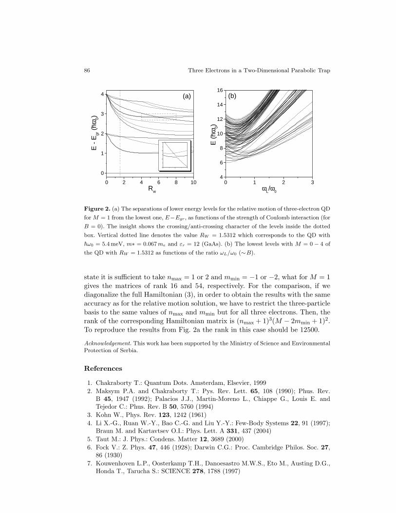
86 Three Electrons in a Two-Dimensional Parabolic Trap
0 2 4 6 8 10
0
1
2
3
4 (a)
|
E -
Egr (
hω0)
Rw
0 1 2 34
6
8
10
12
14
16
|
(b)
E (
hω0)
ωL/ω0
Figure 2. (a) The separations of lower energy levels for the relative motion of three-electron QD
for M = 1 from the lowest one, E−Egr, as functions of the strength of Coulomb interaction (for
B = 0). The insight shows the crossing/anti-crossing character of the levels inside the dotted
box. Vertical dotted line denotes the value RW = 1.5312 which corresponds to the QD with
~ω0 = 5.4meV, m∗ = 0.067 me and εr = 12 (GaAs). (b) The lowest levels with M = 0 − 4 of
the QD with RW = 1.5312 as functions of the ratio ωL/ω0 (∼B).
state it is sufficient to take nmax = 1 or 2 and mmin = −1 or −2, what for M = 1gives the matrices of rank 16 and 54, respectively. For the comparison, if wediagonalize the full Hamiltonian (3), in order to obtain the results with the sameaccuracy as for the relative motion solution, we have to restrict the three-particlebasis to the same values of nmax and mmin but for all three electrons. Then, therank of the corresponding Hamiltonian matrix is (nmax + 1)3(M − 2mmin + 1)2.To reproduce the results from Fig. 2a the rank in this case should be 12500.
Acknowledgement. This work has been supported by the Ministry of Science and EnvironmentalProtection of Serbia.
References
1. Chakraborty T.: Quantum Dots. Amsterdam, Elsevier, 19992. Maksym P.A. and Chakraborty T.: Pys. Rev. Lett. 65, 108 (1990); Phus. Rev.
B 45, 1947 (1992); Palacios J.J., Martin-Moreno L., Chiappe G., Louis E. andTejedor C.: Phus. Rev. B 50, 5760 (1994)
3. Kohn W., Phys. Rev. 123, 1242 (1961)4. Li X.-G., Ruan W.-Y., Bao C.-G. and Liu Y.-Y.: Few-Body Systems 22, 91 (1997);
Braun M. and Kartavtsev O.I.: Phys. Lett. A 331, 437 (2004)5. Taut M.: J. Phys.: Condens. Matter 12, 3689 (2000)6. Fock V.: Z. Phys. 47, 446 (1928); Darwin C.G.: Proc. Cambridge Philos. Soc. 27,
86 (1930)7. Kouwenhoven L.P., Oosterkamp T.H., Danoesastro M.W.S., Eto M., Austing D.G.,
Honda T., Tarucha S.: SCIENCE 278, 1788 (1997)

Few-Body Systems 0, 87–93 (2006) Few-Body
Systemsc© by Springer-Verlag 2006
Printed in Austria
Level Density of the Henon-Heiles System
Above the Critical Barrier Energy∗
M. Brack1,∗∗, J. Kaidel1, P. Winkler2, S. N. Fedotkin1,3
1 Institut fur Theoretische Physik, Universitat Regensburg, D-93040 Regensburg, Germany2 Department of Physics, University of Nevada Reno, NV 89557, USA3 Institute for Nuclear Research, 252028 Prospekt Nauki 47, Kiev-28, Ukraine
Abstract. We discuss the coarse-grained level density of the Henon-Heilessystem above the barrier energy, where the system is nearly chaotic. We useperiodic orbit theory to approximate its oscillating part semiclassically viaGutzwiller’s semiclassical trace formula (extended by uniform approximationsfor the contributions of bifurcating orbits). Including only a few stable andunstable orbits, we reproduce the quantum-mechanical density of states veryaccurately. We also present a perturbative calculation of the stabilities of twoinfinite series of orbits (Rn and Lm), emanating from the shortest libratingstraight-line orbit (A) in a bifurcation cascade just below the barrier, whichat the barrier have two common asymptotic Lyapunov exponents χR and χL.
The two-dimensional Henon-Heiles (HH) Hamiltonian
HHH = T + VHH(x, y) =12
(p2x + p2
y) +12
(x2 + y2) + α (x2y − y3/3) (1)
was introduced [1] to describe the mean gravitational field of a stellar galaxy. Itdescribes an open system in which a particle can escape over one of three barrierswith critical energy Ebar = 1/6α2 and has meanwhile become a textbook example[2, 3, 4] of a system with mixed dynamics reaching from integrable motion (forE → 0) to nearly fully chaotic motion (for E & Ebar). Scaling coordinates andmomenta with α causes the classical dynamics to depend only on the scaledenergy e = E/Ebar = 6α2E; the barrier energy then lies at e = 1.
The Hamiltonian (1) has also been used [5] to describe the nonlinear nor-mal modes of triatomic molecules, such as H+
3 , whose equilibrium configurationhas D3 symmetry. Although this model may no longer be quantitative for largeenergies, it can qualitatively describe the dissociation of the molecule for e > 1.∗Article based on the presentation by M. Brack at the Fourth Workshop on the Dynamicsand Structure of Critically Stable Quantum Few-Body Systems, MPIPKS, Dresden, Germany,2005. Received November 2, 2005
∗∗E-mail address: [email protected]

88 Level Density of the Henon-Heiles System Above the Critical Barrier Energy
In this paper we discuss the coarse-grained level density of the HH Hamilto-nian (1) above the barriers, calculated both quantum-mechanically and semiclas-sically using periodic orbit theory. Since the potential VHH in (1) goes asymp-totically to −∞ like −r3 (r2 = x2 + y2) in some regions of space, the quantumspectrum of (1) is strictly speaking continuous. However, for sufficiently small αthere are quasi-bound states for E < Ebar whose widths are exponentially smallexcept very near Ebar. For semiclassical calculations of the HH level density fore < 1, we refer to earlier papers [6, 7]. In [8] we have calculated the complexresonance energies Em − iΓm by the standard method of complex rotation, di-agonalizing (1) in a finite harmonic-oscillator basis. The level density is, aftersubtracting the non-resonant part of the continuum, given by
∆g(E) = − 1π
Im∑m
1E − Em + i Γm/2
. (2)
We define the coarse-grained level density by a Gaussian convolution of (2) overan energy range γ
∆gγ(E) =1
γ√
π
∫ ∞
−∞∆g(E′) e−(E−E′)2/γ2
dE′, (3)
which can be done analytically [8]. Its oscillating part, which describes the gross-shell structure in the quantum-mechanical level density, is then given by
δgqm(E) = ∆gγ(E)− ∆g(E), (4)
where ∆g(E) is the smooth part of (2) which we have extracted by a complexversion [8] of the numerical Strutinsky averaging procedure [9].
Semiclassically, the quantity δg(E) can be approximated by Gutzwiller’s traceformula [10], which for a system with two degrees of freedom reads
δgscl (E) =1π~
∑po
Tpo(E)rpo
√|TrMpo(E)− 2|
e−[γTpo(E)/2~]2 cos[Spo(E)
~− π
2σpo
]. (5)
The sum goes over all isolated periodic orbits labeled ’po’, and the other quan-tities in (5) are the periods Tpo and actions Spo, the Maslov indices σpo andthe repetition numbers rpo of the periodic orbits. Mpo(E) is the stability matrixobtained by linearization of the equations of motion along each periodic orbit.The Gaussian factor in (5) is the result of a convolution analogous to (3); it sup-presses the orbits with long periods and hence yields the gross-shell structure interms of the shortest periodic orbits, hereby eliminating the convergence prob-lem characteristic of non-integrable systems [3]. This use of the trace formulato describe gross-shell quantum effects semiclassically has found many applica-tions in different fields of physics (including interacting fermion systems in themean-field approximation; see [4] for examples).
The shortest periodic orbits of the classical HH system (1) have already beenextensively studied in earlier papers [11, 12, 13]. In [8] we have calculated allrelevant orbits and their properties from the classical equations of motion and

M. Brack, S. N. Fedotkin, J. Kaidel and P. Winkler 89
-1.0 -0.5 0.0 0.5 1.0
-0.5
0.0
0.5
1.0
y
x e
A5
C3
B4
2
L6
0.9985 0.999 0.9995 1.0
-4
0
4
8
Tr
M
R5R7
R9
L6
A6
L8 L10
A5A7
Figure 1. Left: Contours of the HH potential and some of its shortest periodic orbits in the
(x, y) plane (see text). Right: Trace of the stability matrix of the A orbit and the three pairs of
orbits (R5,L6), (R7,L8), (R9,L10) bifurcated from it, forming the beginnings of the ’HH fans’.
1.0 1.1 1.2 1.3 1.4 1.5 1.6 1.7 1.8 1.9 2.0e
-3.0
-1.5
0.0
1.5
3.0
g(e)
Figure 2. Comparison of quantum-mechanical (solid line) and semiclassical (dashed line) level
density δg(E) of the HH potential versus scaled energy e, coarse grained with Gaussian smooth-
ing range γ = 0.25. Only 18 periodic orbits contribute to the semiclassical result [8].
computed the quantity δgscl(E) in (5). Some of the shortest orbits are shown inthe left part of Fig. 1, all evaluated at e = 1 (except for τ2 which is evaluated ate = 1.1). Note that due to the D3 symmetry of the HH potential, the orbits A5,B4, τ2 and L6 (as well as all orbits Rn and Lm bifurcating from A, see below)have two symmetry partners obtained by rotations about ±2π/3. The orbit C3
and all triplets of Rm orbits have a time reversed partner each.1
In Fig. 2 we show a comparison of semiclassical (5) with quantum-mechanical(4) results, both coarse-grained with γ = 0.25 (units such that ~ = 1). At thisresolution of the gross-shell structure, only 18 periodic orbits contribute to thesemiclassical result; for the period-two orbit D7 which is stable up to e ' 1.29 andinvolves to further orbits (E8, G7) in a codimension-two bifurcation scenario, wehave used the appropriate uniform approximation [14] to avoid the divergenceof the trace formula (5) (see [8] for details). We note that the agreement of1We use here the nomenclature introduced in [12, 13], where the Maslov indices σpo appear assubscripts of the symbols (B4, R5, L6, etc.) of the orbits.

90 Level Density of the Henon-Heiles System Above the Critical Barrier Energy
semiclassics with quantum mechanics is excellent. Only near e ∼ 1 there is aslight discrepancy which is mainly due to some uncertainties in the numericalextraction of ∆g(E). We can conclude that also in the continuum region abovea threshold, the semiclassical description of quantum shell effects in the leveldensity of a classically chaotic system works quantitatively.
In view of the importance of the level density close to the critical barrierenergy e = 1 for the threshold behaviour of a reaction described by the HH modelpotential, we focus now on a particular set of periodic orbits existing at e = 1.The straight-line librating orbit A reaches this energy with an infinite period afterundergoing an infinite cascade of bifurcations for e → 1. At these bifurcations,two alternating infinite sequences of rotational orbits Rn (n = 5, 7, 9, . . .) andlibrating orbits Lm (m = 6, 8, 10, . . .) are born; their bifurcation energies en andem form two geometric progressions converging to e = 1 with a ’Feigenbaumconstant’ δ = exp(2π/
√3) = 37.622367 . . .; the shapes of these new orbits are
self-similar when scaled with√
δ in both x and y direction (see [12] for details).The stability traces of the first three pairs (Rn, Lm) are shown in the right partof Fig. 1. As seen there, the curves TrM(e) of these orbits are nearly linear (atleast up to e ∼ 1.02) and intersect at e = 1 approximately at the same values foreach type (R or L). For large n and m, these values were found numerically [12]to be TrMLm(e = 1) ∼ 8.183 and TrMRn(e = 1) ∼ −4.183. This means that ate = 1, all L orbits have asymptotically the same Lyapunov exponent χL ' 2.087,and all R orbits have the same Lyapunov exponent χR ' 1.368. Based uponthese numerical findings, we postulate the following asymptotic behaviour:
TrMRn,Lm(e) ∼ 2∓ 6.183(
e− e∗
1− e∗
)for e→ 1 , n,m→∞ . (6)
Here e∗ are the respective bifurcation energies of the orbits (en or em), and theminus or plus sign is to be associated with the R or L orbits, respectively. Thecurves TrMRn,Lm(e) thus form two ’fans’ spreading out from the values 8.183 and−4.183 at e = 1, the first three members of each being shown in the right part ofFig. 1. In the following we will sketch briefly how the qualitative features in (6)of these ’HH fans’ can be obtained analytically from semiclassical perturbationtheory. Details will be given in a forthcoming publication [15].
The idea is to start from the following ’separable HH’ (SHH) Hamiltonian
H0 = HSHH =12
(p2x + p2
y) +12
(x2 + y2)− α
3y3 (7)
and to include the term α x2y in first-order perturbation theory. Formally, wemultiply it by a small positive number ε and write HHH = H0 + εH1 withH1 = α x2y = u2v/α2, where u = αx and v = αy are the scaled coordinates. TheHamiltonian (7) is integrable; an analytical trace formula for it has been given in[7]. There is only one saddle at (x, y) = (0, 1) with energy e = 1 and one libratingA orbit along the y axis which undergoes an infinite cascade of bifurcations fore → 1. From it, an infinite sequence of rational tori Tlk bifurcates, where l istheir repetition number and k = 2, 3, . . . counts the bifurcations (and the tori).

M. Brack, S. N. Fedotkin, J. Kaidel and P. Winkler 91
The v motion of the primitive A orbit (l = 1), having uA(t) = 0, is given by
vA(t) = v1 + (v2 − v1) sn2(at, q) , a =
√v3 − v1
6, q =
√v2 − v1
v3 − v1(8)
in terms of the Jacobi elliptic function [16] sn(z, q) with modulus q. In (8),v1 ≤ v2 ≤ v3 are the turning points of the motion along the v axis, defined byVHH(u=0, vi) = e (i = 1, 2, 3). The tori bifurcating at the energies elk have thesame v motion as the A orbit: vT (t) = vA(t). Their u motion is given by
uT (t) =√
(e− elk)/3 sin(t + φ) , e ≥ elk , φ ∈ [0, 2π) . (9)
The angle φ describes the members of the degenerate families of tori.According to semiclassical perturbation theory [17], the actions Slk of the
tori are changed in first order of ε by
δ1Slk(φ) = −ε
∮lk
H1(uT (t), vT (t)) dt = − ε
α2
∫ T(0)lk
0u2
T (t) vT (t) dt , (10)
where T(0)lk = 2πk are the periods of the unperturbed tori [7]. The integral in
(10) takes the form δ1Slk(φ) = Alk + Blk cos(2φ). In the asymptotic limit e→ 1,where q → 1 and TA ∼ ln[432/(1− e)], the coefficients Alk and Blk can be givenanalytically [15]. Integrating the phase shift caused by δ1Slk(φ) over the angle φ(i.e., over the torus Tlk) yields a modulation factor [17] Mlk
Mlk =12π
∫ 2π
0e
i~ δ1Slk(φ) dφ = e
i~ Alk J0(|Blk|/~) , (11)
to be inserted under the sum of tori in the trace formula for the unperturbed SHHsystem given in [7]. Replacing the Bessel function in (11) by its asymptotic formJ0(x) ∼
√2/πx cos(x−π/4) yields two terms for each torus Tlk, corresponding to
the two isolated orbits R and L into which it is broken up by the perturbation.Reading off their overall amplitudes AR,L in the perturbed trace formula andidentifying them with their expression for isolated orbits given in (5), i.e. equating
AR,L =1π~
TR,L
l√|TrMR,L − 2|
(12)
using the unperturbed periods T(0)lk for TR,L, we can determine the perturbative
expression for the stability traces. For the first repetitions (l = 1) they become
TrMRn,Lm(e) ∼ 2∓ 5.069(
e− e1k
1− e1k
)for e→ 1 , (13)
and thus have exactly the same functional form as in (6). Here e1k are thebifurcation energies of the primitive A orbit (l = 1); k = 2, 3, . . . labels the pairsof Rm and Ln orbits with m = 2k + 1 and n = 2k + 2, and the signs are to bechosen as in (6). In (13) we have put ε = 1 which is justified since even for thisvalue the perturbations δ1S1k at e = 1 are sufficiently small.

92 Level Density of the Henon-Heiles System Above the Critical Barrier Energy
Although the perturbative result (13) contains a too small value of the con-stant 5.069 (instead of 6.183) by 18%, it explains qualitatively correctly thenumerical features of the ’HH fans’ in (6), in particular the linear intersection ofthe curves TrMR,L(e) at e = 1 at two values lying symmetrically to TrM = +2.
Acknowledgement. We thank A. G. Magner and L. Wiesenfeld for stimulating discussions. J.K.and S.N.F. acknowledge financial support from the Deutsche Forschungsgemeinschaft (DFG)through the graduate college 638 “Nonlinearity and Nonequilibrium in Condensed Matter”.
References
1. M. Henon and C. Heiles, Astr. J. 69 (1964) 73.
2. G. H. Walker and J. Ford, Phys. Rev. 188 (1969) 416.
3. M. C. Gutzwiller: Chaos in Classical and Quantum Mechanics (Springer,New York, 1990).
4. M. Brack and R. K. Bhaduri, Semiclassical Physics (2nd edition, WestviewPress, Boulder, 2003).
5. N. Fulton, J. Tennyson, D. A. Sadovskiı and B. I. Zhilinskiı, J. Chem. Phys.99 (1993) 906.
6. M. Brack, P. Meier and K. Tanaka, J. Phys. A: Math. Gen. 32 (1999) 331;M. Brack, S. C. Creagh, J. Law, Phys. Rev. A 57 (1998) 788;B. Lauritzen and N. D. Whelan, Ann. Phys. (N. Y.) 244 (1995) 112;M. Brack, R. K. Bhaduri, J. Law, Ch. Maier, M. V. N. Murthy, Chaos 5(1995) 317; ibid. (Erratum) 5 (1995) 707.
7. J. Kaidel and M. Brack, Phys. Rev. E 70 (2004) 016206, ibid. 72 (2005)049903(E).
8. J. Kaidel, P. Winkler and M. Brack, Phys. Rev. E 70 (2004) 066208.
9. V. M. Strutinsky, Nucl. Phys. A 122 (1968) 1;M. Brack and H.-C. Pauli, Nucl. Phys. A 20 (1973) 401.
10. M. C. Gutzwiller, J. Math. Phys. 12 (1971) 343.
11. R. C. Churchill, G. Pecelli and D. L. Rod in: Stochastic Behaviour in Classi-cal and Quantum Hamiltonian Systems, eds. G. Casati and J. Ford (Springer,1979) p. 76;K. T. R. Davies, T. E. Huston and M. Baranger, Chaos 2 (1992) 215;W. M. Vieira and A. M. Ozorio de Almeida, Physica D 90 (1996) 9.
12. M. Brack, Foundations of Physics 31 (2001) 209.
13. M. Brack, M. Mehta and K. Tanaka, J. Phys. A: Math. Gen. 34 (2001) 8199.
14. H. Schomerus, J. Phys. A: Math. Gen. 31 (1998) 4167.
15. S. N. Fedotkin, A. G. Magner and M. Brack, to be published.

M. Brack, S. N. Fedotkin, J. Kaidel and P. Winkler 93
16. M. Abramowitz and I. A. Stegun: Handbook of Mathematical Functions (9thprinting, Dover, New York, 1970)
17. S. C. Creagh, Ann. Phys. (N. Y.) 248 (1996) 60.

Few-Body Systems 0, 94–101 (2006) Few-Body
Systemsc© by Springer-Verlag 2006
Printed in Austria
Wannier-type threshold laws for
multifragmentation and Thomson’s problem∗
V. N. Ostrovsky1∗∗, J. M. Rost2
1 V. Fock Institute of Physics, St. Petersburg State University, 198504 St. Petersburg, Russia2 Max Planck Institute for the Physics of Complex Systems, D-01187, Dresden, Germany
Abstract. Wannier-type threshold theory for multiple break-up processes isbased on the existence of special classical trajectories which represent partialfixed points of the equations of motion in a system of charged particles. Thesetrajectories preserve the shape of the initial configuration while only chang-ing its overall size in time. The relation between such scaling configurationsand Thomson’s (or surface Coulomb) problem is analysed. In particular, it isshown that for eight electrons the twisted cube configuration solves Thomp-son’s problem and also governs the threshold break-up of eight electrons re-ceding from a charged core. The relevant exponents for the threshold powerlaw are evaluated.
1 Introduction
1.1 Scaling configurations
A variety of break-up processes is known in atomic, nuclear and cluster physics.The major difference between nuclear and atomic physics is that in the lattercase generally the fragments have charges of different sign. A special fragmen-tation mechanism in atomic physics for total energies only slightly above thefragmentation threshold was introduced by Wannier [1]. Originally, he treatedthe case of three fragments, namely electron impact ionization of an atom.
Later the ideas were generalized to the situation with an arbitrary numberN of fragments (see Ref. [2] and bibliography therein). The key observation isthat all the fragments have low velocities due to the small excess energy E abovethreshold. Equally important is the notion, that most likely recapture occurs(into a bound excited, i.e., Rydberg state) among a pair of oppositely chargedfragments if their distance increases with time more slowly than other relative∗Article based on the presentations by V. N. Ostrovsky and J. M. Rost at the Fourth Workshopon the Dynamics and Structure of Critically Stable Quantum Few-Body Systems, MPIPKS,Dresden, Germany, 2005. Received November 10, 2005
∗∗E-mail address: [email protected]

V. N. Ostrovsky and J. M. Rost 95
distances. As a result, the desired complete fragmentation is not achieved. Thiscan be avoided, if relative distances and orientations between the fragments arepreserved. Indeed, modern non-linear dynamics methods allow one to describethis break-up processes entirely from the stability properties of a fixed-point forthe equations of motion [3]. The seeming contradiction to describe a fragmen-tation process with particles leaving to infinite distance with a fixed point isresolved by using a scaling argument in excess energy E. Then any finite scaleddistance r/E tends to infinity if the excess energy approaches threshold E → 0.
In a less abstract but essentially equivalent formulation the fragments forma scaling configuration (SC) in time [2]. It blows up while its shape is retainedaccording to
rj(t) = φ(t)ρj , (1)
where rj(t) are time-dependent vector of the (j = 1, 2, . . . N) fragments withrespect to the centre of mass (CM) of the system. Implying a classical descriptionfor the motion of the fragments, the Coulomb interaction, Eq. (1) reduces themulti-dimensional problem to that for a single degree of freedom, φ(t), witheffective Hamiltonian [2]
H0 =12M
(dφ
dt
)2
− Q0
φ, (2)
and initial condition φ(t0) = 1 and φ(t0) determined via Eq. (2) through energyconservation. Clearly, the dynamics of φ(t) must depend on the initial shapegiven by the rj(t0) = φ(t0)ρj = ρj . The initial shape determines parametersin the dynamic equation (2): the “effective mass” M =
∑Nj=1 mjρ
2j and the
“effective charge” Q0 = −∑
i>j qiqj |ρi − ρj |−1, where mj and qj are mass andcharge of the j-th fragment, respectively. To remain shape-invariant the initialconfigurations ρj need to satisfy a SC conditions [2]
αρj = − 1mj
∑k 6=j
qjqkρj − ρk
|ρj − ρk|3, (3)
that ensure that acceleration of each particle rj is proportional to its CMS vectorrj , as follows from formula (1); α = Q0/M. An alternative, albeit equivalentformulation of the fixed-point condition is provided in the subsection 1.2.
It is universally known that the classical three- (or more) body problem doesnot allow analytical solution for a general initial condition. However this doesnot exclude possibility of SC analytical solutions (1) for some special initial con-ditions rj(t0) = ρj . Propagation along an expanding SC is the most efficientpathway to achieve full fragmentation given a small energy excess E. The actualtrajectories leading to near–threshold fragmentation approach the SC configu-ration and their volume in phase space determines the cross section in the formthe Wannier-type power law, σ ∼ Eµ. More precisely, the threshold exponentµ =
∑µj is a sum of partial indices µj which characterize the instability of the
SCs, for details, see [2, 3].

96 Wannier-type threshold laws and Thomson’s problem
1.2 Scaling configurations and hyperspherical coordinate basis
Additional insight is obtained by considering the problem in hyperspherical co-ordinates where the SCs have an intuitive meaning [2, 4, 3]. In these coordinatesthe potential energy is cast in generalized Coulomb form
V =∑i<j
qiqj
rij=
C(Ω)R
, (4)
where the hyperradius is defined by R2 =∑N
j mjr2j . The hypercharge C(Ω)
depends on a set of hyperangles Ω = Ω1, Ω2, . . . Ω3N−7 which might be chosenin different ways (see, e.g., [5]). The set of hyperangles defines all geometricalangles in a configuration of particles and also all the ratios of distances betweenthe fragments.
By definition, for an SC, all hyperangles have fixed values in time, Ω(0) =Ω(0)
1 , Ω(0)2 , . . . Ω
(0)3N−7. Such a trajectory is possible only provided Ω(0) is sta-
tionary, i.e., a fixed point of C(Ω) on the hypersphere,
∂C(Ω)∂Ωj
∣∣∣∣Ω=Ω(0)
= 0 , j = 1, 2, . . . (3N − 7) . (5)
Note, that the stationary point cannot correspond to a stable equilibrium. This isthe dynamic analogue [2] of the well known Earnshow theorem in electrostatics.The conditions (3) or (5) present two equivalent sets of non-linear equations; nosystematic methods of solution are known.
It is easy to establish relation with parameters introduced in Section 1.1.With φ(t0) = 1, we find R(t0)2 =
∑Nj mjρ
2j = M, C(Ω0) = R(t0)Q0 = M1/2Q0.
The partial threshold indices µj characterize the instability of the saddle pointΩ(0) on the hypersphere [2].
2 Scaling configurations and Thomson’s problem
2.1 Thomson’s problem
The problem of finding SCs is similar to Thomson’s famous problem (TP), alsoknown as the surface Coulomb problem. It was put forward by J. J. Thomson inconnection to his plum pudding model of an atom [6]. The problem belongs toelectrostatics and implies to find the global minimum of potential energy for Nidentical point charges confined to the surface of a sphere, i.e. minimizing Eq. (4)under conditions qj = 1, |rj | = 1 (hereafter a unit charge and a unit sphere areassumed). The related configuration of classical charged particles is referred tobelow as Thomson’s configuration (TC). Notwithstanding its elementary physicalformulation, TP exhibits a variety of quite unexpected properties and servesas a testground for complexity studies. The literature on the problem (and itsgeneralizations and extensions) is vast, ranging from mathematically rigorousstudies to physical, chemical and biological applications; we give here only somerepresentative references [7, 8, 9, 10, 11, 12, 13, 14, 15, 16, 17, 18, 19, 20, 21].

V. N. Ostrovsky and J. M. Rost 97
Table 1. Comparison of Thomson’s problem and scaling configurations problem.
Thomson’s problem Scaling configuration problem
Charged particles confined to a sphere Charged particles on a hypersphere
Search for a particle configuration thatprovides a minimum of interaction po-tential
Search for a particle configuration thatprovides a saddle point (minima do notexist)
Many configurations provide localminima
Many configurations provide saddlepoints
Global minimum is of interestScaling configuration that providesminimum threshold index µ is of in-terest
2.2 Comparison of scaling and Thomson’s configurations
The objective of the present study is a comparative discussion of TCs and SCs,a summary is provided in table 1. For TCs one has to locate the minima ofpotential energy for the charged particles confined to a sphere in real space. Indistinction, for SCs the stationary points (or saddle points) on a hypersphere areof interest. In simple terms this means that in the second case the particles areallowed to be at different distances from the center yet compatible with the fixedpoint condition Eq. (5).
In the TP the number of stationary points seems to increase exponentiallywith the number N of particles [14]. The same applies to the SCs problem. Thereis no analytical solution to identify the global minimum of the interaction energyV . For small N the TCs can be found in different sources [14, 18, 21]. For largeN the problem is solved numerically by various trial and error methods; large-Nasymptotic expressions for the energy are discussed in [11, 14, 16]. Numericalfinding of SCs is even more difficult, since the gradient methods do not work.When SCs are applied in the threshold law theory, one has to select the optimumscaling configuration (OSC) that yields the minimum threshold exponent µ [2].
2.3 Special values of N
TCs and SCs are identical in case N = 3 (triangle) and N = 4 (tetrahedron,which is Platonic solid). The competing SCs with larger µ, respectively, are aline (for N = 3) and a line and a square (for N = 4).
For N = 5 the TC and SC are different. In both cases they are bypiramidsformed by equilateral triangles with the other two particles located symmetricallyabove and below the triangle. For the TP, when all charges lie on a sphere, theangle α at the pyramids vertices is equal to 45. For the SC problem the angle α isa variable parameter to be defined from the SC conditions Eq. (5). The equationthat governs α was derived in Ref. [2] for a more general situation when a chargeZ of opposite sign is placed in the centre of SC (such a charge does not influenceTC). Table 2 lists values of α for different Z. They prove to be surprisingly closeto 45, albeit slightly less; they tend to 45 as Z increases. Hence, although forthe SCs the particles are not forced to lie on a sphere, in fact for N = 5 the SCs

98 Wannier-type threshold laws and Thomson’s problem
Z α5 α7
0 44.40165 45.7899
2 45.15762a 44.4655
3 45.09672a 44.7121
4 45.06976a 44.8028
5 45.05455a 44.8500b
6 45.04479a 44.8789b
7 45.03799a 44.8985b
8 45.03298 44.9126b
9 45.02914 44.9233b
10 45.02610 44.9317b
Table 2. Parameters of scaling configuration
(bipyramids) α5 for six-particle systems A+Z +
5e and α7 for eight-particle systems A+Z + 7e;
a – results from Ref. [2]; b – results from
Ref. [22].
prove to be very close to spherical.A similar situation emerges for N = 7 where both TC [18] and SC [22] are
symmetrical bypiramids with a pentagon as a base. In this case the SC canalso be characterized by a single angle α [22]. It is slightly larger than 45 andapproaches 45 for Z →∞. For N = 6 both TC and SC are octahedron (Platonicsolid). The case N = 8 is considered in the next section.
For some values of N the TCs correspond to the charge distributions with anon-zero dipole moment (the lowest value is N = 11). Such a situation cannotoccur for the SCs of identical particles, since the CM frame is pre-chosen.
3 Configurations with eight charges
For N = 8 equal charges the highly symmetrical cubic arrangement (Platonicsolid) is an obvious candidate for the TC or SC. However, this configurationprovides only a saddle point for the potential energy V ; the minimum is ensuredby the twisted cube (known also as the compressed square antiprism). Transitionfrom the cube to the twisted cube can be divided into two steps. First, upperplane with four charges is rotated by an angle β relative to the lower plane.The lowest energy is obtained for βt = 45. Second, further energy loweringis achieved if the distance 2a between the planes is considered as a variableparameter (it is assumed that all the charges remain on a unit sphere whosecentre lies symmetrically between the planes). The equation that governs a reads
(2 +√
2)√
1− a2
[2−√
2 + (2 +√
2)a2]3/2+
(2−√
2)√
1− a2
[2 +√
2 + (2−√
2)a2]3/2− 2
√2 + 1
4(1− a2)= 0 . (6)
Its solution is at = 0.5604367652904, while the regular cube corresponds toac = 1/
√3 = 0.57735027. The twisted cube provides the global minimum for V
[8, 18, 21] with a potential energy (qj ≡ 1) Vt = 19.67528786123277 which is by0.33% lower than Vc = 19.74077407376279 for the regular cube. The surface ofV as function of the collective coordinates β and a is shown in figure 1.
The fact that the twisted cube provides TC does not necessarily mean that itserves also as the OSC. Nevertheless, experience with the TC hints at consideringthe twisted cube as a competing candidate for OSC. The results of our calcula-tions of partial µj and total µt threshold indices within the general framework

V. N. Ostrovsky and J. M. Rost 99
-40-20 0 2040
Β
0.5250.55
0.5750.6
0.625
a
19.7
19.75
19.8
V
19.7
19.75
Figure 1. Surface of potential en-
ergy V (4) for the system of N =
8 charges as function of two collec-
tive coordinates β and 2a (see text
for detail). The regular cube corre-
sponds to the saddle point β = 0,
ac = 0.5774, while twisted cube cor-
responds to β = 45, at = 0.5604.
Table 3. Partial µj and total µt threshold indices for nine-particle systems A+Z + 8e. The
scaling configuration is twisted cube. The number in parentheses indicates degree of unstable
mode degeneracy. µc is threshold index for regular cube as the scaling configuration [22].
Z µ1 µ2 µ3 µ4 µt µc
6 1.26687 (2) 1.24883 (2) 1.19876 1.19849 (2) 8.62711 8.657987 1.21226 (2) 1.19768 (2) 1.15719 1.15695 (2) 8.29096 8.315228 1.17628 (2) 1.16403 (2) 1.13002 1.12979 (2) 8.07022 8.090229 1.15075 (2) 1.14019 (2) 1.11086 1.11066 (2) 7.91406 7.9310910 1.13170 (2) 1.12242 (2) 1.09663 1.09644 (2) 7.79774 7.8125611 1.11693 (2) 1.08647 (2) 1.08563 1.08546 (2) 7.70770 7.72083
of Ref. [2] are shown in table 3 for different values of the central charge Z (theSC parameters βt and at do not depend on Z). Comparison with the results µc
for the regular cube [22] reveal that the twisted cube is the OSC. Interestingly,not only total threshold index µ, but also all partial indices µj for the twistedcube are smaller than for the regular cube.
The threshold indices µt in table 3 describe the electron impact fragmentationprocess
e + Aq → AZ + 8e , Z = q − 7 , (7)
or photofragmentation
γ + Aq → AZ + 8e , Z = q − 8 . (8)
Since these indices correspond to OSC, these indices are to be used instead oflarger indices µc obtained in Ref. [22] for cubic configuration. The lowering of µis relatively small and difficult to observe experimentally; still it is of principleinterest. Concerning experimental observations of the Wannier-type thresholdlaws in electron impact ionization (or photoionization) of atoms it is worthy toindicate that they can be masked by the secondary threshold laws in case whenthe residual ion is a multielectron system [23]. However if the residual core is abare atomic nucleus, then the resonance secondary mechanism is not operative.

100 Wannier-type threshold laws and Thomson’s problem
4 Conclusion
We have discussed the analogy between the well studied Thomson problem andthe threshold fragmentation of charged particles using the description of scalingconfigurations of the latter as a bridge. While there are specific differences, so-lutions of Thomson’s problem can guide the difficult search for optimal scalingconfigurations in high dimensions as demonstrated here with the twisted cubefor 8-fold ionization of an atom or ion.
Possible generalizations include the threshold problem for fragments inter-acting by a dipole-like potential ∼ r−2
ij [24]. A similar analogue of Thomson’sproblem was studied by a number of authors [14]. In the quantum TP (notconsidered previously) one has to treat charges as quantum particles. Here aninteresting feature is resonance tunnelling between equivalent minima (see Fig. 1)that leads to splitting of energy levels, similarly to internal rotation in molecules.
Acknowledgements
The authors are thankful to K. B. MacAdam for attracting their attention toThomson’s problem.
References
1. G. H. Wannier, Phys. Rev. 90, 817 (1953).
2. M. Yu. Kuchiev and V. N. Ostrovsky, Phys. Rev. A 58, 321 (1998).
3. J.-M. Rost, Physica E 9, 467 (2001).
4. J.-M. Rost, Phys. Rep. 297, 271 (1998).
5. U. Fano, D. Green, J. L. Bohn, and T. A. Heim, J. Phys. B 32, R1 (1999).
6. J. J. Thomson, Phil. Mag. 44 (ser. 5), 293 (1897); 7 (ser. 6), 237 (1904).
7. J. Foppl, J. Reine Angew. Math. 141, 251 (1912); L. L. Whyte, Am. Math.Month. 59, 606 (1952); J. Leech, Math. Gazette 41, 81 (1957).
8. E. Marx, J. Franklin Inst. 290, 71 (1970);
9. T. W. Melnyk, O. Knop, and W. R. Smith, Can. J. Chem. 55, 1745 (1977).
10. N. Ashby and W. E. Brittin, Am. J. Phys. 54, 776 (1986); T. Erber andG. M. Hockney, J. Phys. A 24, L1369 (1991); L. Glasser and A. G. Every, J.Phys. A 25, 2473 (1992); N. N. Andreev, East J. Approx. 2(4), 459 (1996).
11. V. A. Yudin, Discretnaya Matematika 4(2), 115 (1992) (in Russian); Discr.Math. Appl. 3(1), 75 (1993).
12. T. Erber and G. M. Hockney, Phys. Rev. Lett. 74, 1482 (1995).
13. J. R. Morris, D. M. Deaven, and K. M. Ho, Phys. Rev. B 53, R1740 (1996);

V. N. Ostrovsky and J. M. Rost 101
14. T. Erber and G. M. Hockney, Adv. Chem. Phys. XCVIII, 495 (1997).
15. A. Perez-Garrido, M. J. W. Dodgson, M. A. Moore, M. Ortuno, and A. Daz-Sanchez, Phys. Rev. Lett. 79, 1417 (1997); A. Perez-Garrido, M. J. W. Dodg-son, and M. A. Moore, Phys. Rev. B 56, 3640 (1997); E. L. Altschuler,T. J. Williams, E. R. Ratner, R. Tipton, R. Stong, F. Dowla, and F. Wooten,Phys. Rev. Lett. 78, 2681 (1997).
16. E. A. Rakhmanov, E. B. Saff, and Y. M. Zhou, Math. Res. Lett. 1, 647(1994); A. B. J. Kuijlaars and E. B. Saff, Trans. Am. Math. Soc. 350, 523(1998).
17. A. Perez-Garrido and M. A. Moore, Phys. Rev. B 60, 15628 (1999).
18. A. M. Livshits and Yu. E. Lozovik, Chem. Phys. Lett. 314, 577 (1999).
19. M. Bowick, A. Cacciuto, D. R. Nelson, and A. Travesser, Phys. Rev. Lett.89, 185502 (2002); E. L. Altschuler and A. Perez-Garrido, Phys. Rev. E 71,047703 (2005).
20. A. A. Berezin, J. Electrostatics 40&41, 79 (1997); K. B. MacAdam andC. S. Hwang, Rev. Sci. Inst. 74, 2267 (2003).
21. The TCs with N ranging from 1 to 24 are presented and discussed at theInternet site http://www.mathpages.com/home/kmath005.htm.
22. V. N. Ostrovsky, J. Phys. B 37, 4657 (2004).
23. G. F. Gribakin, S. Sahoo, and V. N. Ostrovsky, Phys. Rev. A 70, 062717(2004).
24. T. Pattard and J. M. Rost, Found. Phys. 31, 535 (2001).

Few-Body Systems 0, 102–107 (2006) Few-Body
Systemsc© by Springer-Verlag 2006
Printed in Austria
Mass-Related Dynamical Barriers in
Triatomic Reactions∗
T. Yanao, W. S. Koon, and J. E. Marsden
Control and Dynamical Systems, MC 107-81, California Institute of Technology, Pasadena,CA 91125, USA
Abstract.A methodology is given to determine the effect of different mass distri-
butions for triatomic reactions using the geometry of shape space. Atomicmasses are incorporated into the non-Euclidean shape space metric after theseparation of rotations. Using the equations of motion in this non-Euclideanshape space, an averaged field of velocity-dependent fictitious forces is de-termined. This force field, as opposed to the force arising from the potential,dominates branching ratios of isomerization dynamics of a triatomic molecule.This methodology may be useful for qualitative prediction of branching ratiosin general triatomic reactions.
1 Introduction
The roles played by atomic masses are of great interest in current chemicalphysics. Atomic-mass effects will be the most prominent in isotopic reactionssuch as the breakup dynamics of triatomic hydrogen ion H+
3 and its isotopomers,D2H+, H2D+, and D+
3 [1]. The anomalous isotope effect in ozone O3 [2, 3] alsoprovides intriguing problems that are related to the influence of atomic masses.Therefore, a general framework to describe the effect of atomic masses in tri-atomic reactions should serve many purposes.
Atomic masses are incorporated into the metric tensor of shape space onthe basis of reduction theory [4] and gauge theory [5, 6, 7] that is used for theseparation of rotational degrees of freedom. The metric tensor after reductionis generally non-Euclidean for three- and more-atom systems. As a result, thedynamical effects that have their origin in the non-Euclidean nature of the metricof shape space, should be important for understanding the effect of the masses.It should be noted that while the Born-Oppenheimer potential energy surface∗Article based on the presentation by W.S. Koon at the Fourth Workshop on the Dynamicsand Structure of Critically Stable Quantum Few-Body Systems, MPIPKS, Dresden, Germany,2005. Received November 14, 2005; Accepted December 6, 2005

T. Yanao, W. S. Koon, J. E. Marsden 103
changes depending on the system, the geometry of shape space is rather intrinsicand independent of the system. Therefore, it is important to study the geometryof shape space of many-body systems.
Its non-Euclidean nature suggests that trajectories in shape space possess acertain directionality, even without the influence of the potential energy surface.This directionality is of importance in branching processes in multi-channel re-actions. The behavior of geodesics signals this “preference” of motion in shapespace. In this article, using suitable coordinates, an averaged field of “fictitiousforces” is found that accounts for the directionality of geodesics. It is shownthat this force field does, in fact, dominate mass-influenced branching ratios ofisomerization dynamics of a triatomic molecule.
A prototypical model to study mass-related branching ratios of isomeriza-tion reactions is presented in §2, and §3 gives a theoretical explanation for thebranching ratios via the geometry of shape space.
2 Model Reactions and Branching Ratios
This section investigates the isomerization dynamics of a molecular cluster com-posed of three atoms with different masses (m1,m2,m3) = (1, 1, 0.1) with theaim of determining the effects of the values of the masses. The total angular mo-mentum of the system is taken to be zero for simplicity. The three atoms interactequally through a pairwise Morse potential. Because of the mass difference, thissystem is called a “modified” M3 cluster. The dimensionless Hamiltonian of thesystem is given by
Hε
=12m1r
21 +
12m2r
22 +
12m3r
23 +
∑i<j
[e−2(dij−6) − 2e−(dij−6)
], (1)
where ri = (rix, riy, riz)T (i = 1, 2, 3) is the three dimensional position vector of
each atom. Here, ε represents the depth of the Morse potential and dij is theinter-particle distance between the i-th and j-th atoms. In what follows, ournumerical results are presented in absolute units.
As shown in Fig. 1(a), this cluster has two local equilibrium structures (iso-mers) whose potential energy is V = −3.00ε. These are equilateral triangle andpermutationally distinct since motion of the system is confined to a plane be-cause of the assumption of zero total angular momentum. The system has threesaddle points with potential energy V ≈ −2.005ε, which correspond to collinearconfigurations. They are also permutationally distinct. Channel 1 and Channel2 are essentially equivalent and only Channel 3 is different from the other two.The potential-barrier heights for these three channels are exactly the same sincethe three particles interact equally through the pairwise Morse potential. Thedifference lies in the effect that different masses have on the dynamics of theisomerization reactions.
Fig. 1(b) shows the energy dependence of the relative reaction frequencies forthe respective channels. In this numerical experiment, the frequencies of reactionsthrough respective channels are counted and normalized to 100. To avoid over-counting reactions due to recrossing, only the event in which the system leaves

104 Mass-Related Dynamical Barriers in Triatomic Reactions
(a)
0 20
40 60
80 100 -40 -20 0 20 40
-20
0
20
w1 w2
w3
1 2
3
1 32
1 2 3
1 2
3
Channel 1
Channel 2
12 3
Channel 3
+020
4060
80
100-40 -20 0 20 40
-20
0
20
2040
6080
100
w1
w2
w3 +
0
10
20
30
40
50
60
-2 -1.8 -1.6 -1.4 -1.2 -1
Energy (ε)
Rel
ativ
e fr
eque
ncy
(%)
Channel 3
Channel 1 & 2
(b)
Figure 1. (a) Two equilibrium configurations and three saddle configurations of the modified
M3 cluster. The curves are the steepest descent paths of the potential energy. The two equilib-
rium points are located at (w1, w2, w3) = (15.429, 0,±13.607). The saddle point for Channel 1
is at (10.277, 23.548, 0) while that for Channel 2 is located at (10.277,−23.548, 0). The saddle
point for Channel 3 is at (71.939, 0, 0). Inset is the equi-potential surface at V = −1.4ε. (b)
Energy dependence of relative reaction frequency for each channel.
the vicinity of one of the equilibrium points and arrives at the vicinity of theother equilibrium point is counted. It is evident from Fig. 1(b) that the reactionthrough Channel 3 is much less frequent than those through Channels 1 and2. In other words, the system prefers the reaction through heavy-heavy-lightconfigurations rather than heavy-light-heavy configurations. Furthermore, thistendency is observed to become more prominent as the energy of the systemincreases. The bias in the reaction frequency in Fig. 1(b) cannot be explainedsimply by the potential energy barrier height since the barrier height for thethree channels are the same. Instead, the bias must be related to the mass. Inthe next section, a possible explanation for this mass effect is given.
3 Geometry of Shape Space and Dynamical Barriers
A useful coordinate system for characterization of mass effect in triatomic reac-tions is the so-called “symmetrical coordinates” [6, 7], which is defined as follows.First, the mass-weighted Jacobi vectors are defined as
ρ1 =√
µ1 (r1 − r2) , ρ2 =√
µ2
(m1r1 + m2r2
m1 + m2− r3
), (2)
where µ1 = m1m2/(m1 + m2) and µ2 = (m1 + m2)m3/(m1 + m2 + m3) are thereduced masses. Then the shape (internal) coordinates are defined as,
w1 = |ρ1|2 − |ρ2|2 , w2 = 2ρ1 · ρ2, w3 = 2ρ1 × ρ2, (3)
where the sign of w3 specifies the permutational isomers of the modified M3 clus-ter. Fig. 1(a) shows the steepest descent paths of the potential energy connecting

T. Yanao, W. S. Koon, J. E. Marsden 105
the two equilibrium points via the three saddle points. The inset shows the equi-potential surface of the modified M3 cluster at V = −1.4ε. The interior regionof the equi-potential surface is called “Hill’s region” in analogy with usage inastrophysics. The structures in Fig. 1(a) have reflection symmetry with respectto the w1-w2 plane and the w1-w3 plane.
The intrinsic metric tensor of shape space for the coordinates (w1, w2, w3)is known to be diagonal [6, 7] with g11 = g22 = g33 = 1/4w, where w =√
w21 + w2
2 + w23 and gij = 0 (for i 6= j). Therefore the Lagrangian for the
triatomic system with zero-angular momentum is
L =12
(1
4w
)w2
1 +12
(1
4w
)w2
2 +12
(1
4w
)w2
3 − V (w1, w2, w3). (4)
Then classical equations of motion derived from this Lagrangian are
14w
w1 −w1
8w3w2
1 +w1
8w3w2
2 +w1
8w3w2
3 −w2
4w3w1w2 −
w3
4w3w1w3 = − ∂V
∂w1, (5)
14w
w2 +w2
8w3w2
1 −w2
8w3w2
2 +w2
8w3w2
3 −w1
4w3w2w1 −
w3
4w3w2w3 = − ∂V
∂w2, (6)
14w
w3 +w3
8w3w2
1 +w3
8w3w2
2 −w3
8w3w2
3 −w2
4w3w3w2 −
w1
4w3w3w1 = − ∂V
∂w3. (7)
The terms from the 2nd to the 6th on the left hand sides of these equations arequadratic in the velocity components wi. These terms are originated from thenon-Euclidean metric of shape space and can be regarded as velocity-dependent“fictitious forces” in the coordinate chart depicted in Fig. 2. These terms char-acterize the behavior of geodesics.
To extract the essential property of these velocity-dependent force terms,their averages are considered. This is reasonable since these velocity-dependentterms (forces) usually fluctuate rapidly in the chaotic dynamics of the system.If the distribution of velocity vectors in the tangent space at each point is suffi-ciently stochastic, then the equipartition law holds for the kinetic energy termsin Eq. (4). As a result, one obtains, for the averages of the diagonal quadraticterms,
⟨w2
1
⟩=
⟨w2
2
⟩=
⟨w2
3
⟩= 8wK/3, where K = E − V (w1, w2, w3) is the
kinetic energy at each point in the shape space. As for the cross terms, one gets〈wiwj〉 = 0 (for i 6= j), since one can assume wi and wj are independent in astochastic system. Applying these averages to the velocity-dependent terms inEqs. (5)-(7), an averaged force field is finally obtained as(
−Kw1
3w2,−Kw2
3w2,−Kw3
3w2
). (8)
This force field should be working effectively in the dynamics of the cluster.Fig. 2(a) shows the field of Eq. (8) in the Hill’s region at E = −1.4ε. Ob-
serve that the averaged force works to block trajectories to get into the reactionpathway of Channel 3 at the vicinity of the two equilibrium points. This is themass-related dynamical barrier originated from the geometry of shape space. Toquantify the effects of the averaged force, a “reaction-path potential” is intro-duced, which is defined as the sum of the original potential and the line-integral

106 Mass-Related Dynamical Barriers in Triatomic Reactions
0 20
40 60
80 100 -40 -20 0 20 40
-20
0
20
w1w2
w3
Channel 1 Channel 2
Channel 3
+
-3
-2.8
-2.6
-2.4
-2.2
-2
-1.8
-1.6
-1.4
-1.2
0 1 2 3 4 5 6 7-3
-2.8
-2.6
-2.4
-2.2
-2
-1.8
-1.6
-1.4
-1.2
0 2 4 6 8 10
Arc-length
Ener
gy(ε
)
s
Channel 1 & 2 Channel 3(b)
Ener
gy(ε
)
Arc-length s
(a)
Figure 2. (a) Field of the averaged fictitious force in Hill’s region at E = −1.4ε. (b) Solid lines
are the original potential for respective reaction channels. The broken lines and the dotted lines
are the reaction-path potential at total energy E = −1.8ε and E = −1.4ε respectively.
of the averaged force along a path. For simplicity, the steepest descent paths arechosen in Fig. 1(a) as the reaction paths. Fig 2(b) shows the original potentialand the reaction-path potential as a function of arc-length of the path for re-spective channels. The height of original potential barrier is the same for all thechannels. The barrier of reaction-path potential becomes higher and higher as theenergy increases in Channel 3, while the energy dependence of the reaction-pathpotential is very weak for Channel 1 and 2. This explains why the isomerizationreaction through Channel 3 becomes much less frequent as the energy increases.
In conclusion, a concise method to characterize the effect of different massesfor triatomic reactions has been proposed. An averaged force field has been de-duced using the non-Euclidean metric of shape space. This force field is shown toplay a crucial role in determining the mass-related branching ratios of isomeriza-tion of the triatomic cluster. Since the geometry of shape space is independent ofthe system, the proposed methodology should be useful for varieties of triatomicreactions.
Acknowledgement. This work was partially supported by NSF-ITR grant ACI-0204932, ICB-ARO grant DAAD19-03-D-0004, NSF-DMS-0505711, and JSPS Research Fellowships.
References
1. Datz, S., Larsson, M., Stromholm, C., Sundstrom, G., Zengin, V., Danared,H., Kallberg, A., af Ugglas, M.: Phys. Rev. A52, 2901 (1995)
2. Gao Y. Q., Marcus R. A.: Science 293, 259 (2001)
3. Grebenshchikov, S. Y., Schinke, R., Fleurat-Lessard, P., Joyeux, M.: J.Chem. Phys. 119, 6512 (2003)
4. Marsden, J. E., Ratiu, T. S., Scheurle, J.: J. Math. Phys. 41, 3379 (2000)
5. Guichardet, A.: Ann. Inst. H. Poincare 40, 329 (1984)
6. Iwai, T.: J. Math. Phys. 28, 1315 (1987)

T. Yanao, W. S. Koon, J. E. Marsden 107
7. Littlejohn, R. G., Reinsch, M.: Rev. Mod. Phys. 69, 213 (1997)

Few-Body Systems 0, 108–113 (2006) Few-Body
Systemsc© by Springer-Verlag 2006
Printed in Austria
Application of Tube Dynamics to
Non-statistical Reaction Processes∗
F. Gabern1,2, W.S. Koon2, J.E. Marsden2, S.D. Ross3, and T. Yanao2
1 Departament de Matematica Aplicada I, Universitat Politecnica de Catalunya, Av. Diago-nal, 647, 08028 Barcelona, Spain
2 Control and Dynamical Systems, California Institute of Technology, MC 107-81, Pasadena,CA 91125, USA
3 Department of Aerospace and Mechanical Engineering, University of Southern California,RRB 217, Los Angeles, CA 90089-1191, USA
Abstract. A technique based on dynamical systems theory, is introduced forthe computation of lifetime distributions and rates of chemical reactions andscattering phenomena, even in systems that exhibit non-statistical behavior.In particular, we merge invariant manifold tube dynamics with Monte Carlovolume determination for accurate rate calculations. This methodology is ap-plied to a three degree of freedom model problem and some ideas on how itmight be extended to higher degree of freedom systems are presented.
1 Introduction
Chemical reaction rates are usually computed using statistical methods, such asRice-Ramsperger-Kassel-Marcus (RRKM) theory, also known as transition statetheory (TST). TST is based on the identification of a transition state (TS) be-tween regions of phase space that correspond to either “reactants” or “products.”TST yields rates based on a local study of the TS as well as the assumption thatthe phase space in each region is structureless. These values can be several ordersof magnitude off of experimental values [1]. Despite its shortcomings, TST hasbeen a workhorse of the chemistry community for decades. However, it is nowwell known that while the structureless assumption is useful in many situations,in general these regions (often defined by potential wells) are not structureless.
Many attempts have been made to remedy this situation. De Leon et al. [2]attempted to extend the local picture near the TS in two degree of freedom(dof) systems to a more global one and developed reaction island theory usingcylindrical manifolds. Komatsuzaki and Berry [3] used perturbative methods to∗Article based on the presentation by F. Gabern at the Fourth Workshop on the Dynamicsand Structure of Critically Stable Quantum Few-Body Systems, MPIPKS, Dresden, Germany,2005, Received November 14 2005; Accepted December 1, 2006

Gabern, Koon, Marsden, Ross, and Yanao 109
study the transition near the saddle region. Uzer et al. [4] studied the localgeometric structures of rank-one saddles that regulate reactions in systems withthree or more dof. But a comprehensive theory of chemical reactions and efficientcomputational tools for reaction rate calculations in three or more dof systemswhich takes into consideration phase space structures still needs to be developed.
By merging tube dynamics of Koon el al. [6] and De Leon et al. [2] withMonte Carlo methods, [5] provides some enabling theoretical and computationaltools for the computation of lifetime distributions and rates of chemical reactionsand scattering phenomena. The standard RRKM assumption of an unstructuredphase space fails to account for the dynamics of systems exhibiting significantnon-statistical behavior. This difficulty is overcome by using the homoclinic andheteroclinic intersection structure of tubes in phase space developed in [6].
A main problem with the application of tube dynamics has been the compu-tation of volumes of tube intersections in phase spaces of high dimension [2, 4].The paper [5] provides a starting point for overcoming this hurdle with an algo-rithm that uses tube dynamics to provide the initial bounding box for a MonteCarlo volume determination. We apply the method to a model three dof prob-lem in which the hypotheses of TST do not hold: namely, the full-scattering ofelectrons of Rydberg hydrogen atoms in crossed electric and magnetic fields. Weuse a variety of methods and software that have been developed for tube dynam-ics [6, 7] to better understand the transport between different regions of phasespace. The numerical results obtained are a demonstration of accurate lifetimedistribution and rate calculations which overcome some of the difficulties of thestandard statistical methods. Moreover, we mention some of our current effortin extending the applicability of our computational methods.
2 Merge Tube Dynamics with Monte Carlo Methods
Many chemical reactions proceed through energetic barriers. Such situations arewell described in phase space where the energy-fixed hyper-surface determinesdifferent regions connected by the energy barriers, specifically by structures re-lated to rank-one saddles associated with the barriers. To simplify the discussion,we consider a two state system where one state is bound and the other is un-bound. Figure 1(a) shows a planar projection of the Hill region for the Rydbergatom in crossed fields; this Hill region shows the region in configuration spacewhere the motion of the electron is possible for a given energy level.
The ionization of a Rydberg hydrogen atom in external crossed electric andmagnetic fields has been studied by other authors (such as [4]). To illustrateour method, we investigate the full-scattering problem, in which the system isprepared in an unbound initial state and we study the dynamics of formationof an excited Rydberg atom and its subsequent ionization. The dynamics of theoutermost electron can be described by the following classical Hamiltonian:
H =12(p2
x + p2y + p2
z)−1r
+12(xpy − ypx) +
18(x2 + y2)− εx,
where r =√
x2 + y2 + z2 is the distance from the electron to the center of thenuclear core and ε is the scaled electric field strength.

110 Application of Tube Dynamics to Non-statistical Reaction Processes
Figure 1. (a) Stable/Unstable (W s,u± ) tubes of the NHIM in the bound RB and the unbound
region RU . Σh denotes the Poincare section. (b) xx projection of the intersection of the high-
dimensional tubes with the Poincare section: the entrance (dark one) and the exit (light one).
For an energy value just above that of a saddle, the bottleneck near thesaddle opens (see Figure 1(a)) and the electron can move between the unboundand bound region. Specifically, in the bottleneck region, there exist 4 types oforbits: (i) a large number of bounded orbits which form a topological 3-sphere,i.e., instead of a periodic orbit S1 in the 2dof case, we have a S3 of boundedorbits in the 3dof case; it is an example of a normally hyperbolic invariant mani-fold (NHIM) where the stretching and contraction rates transverse to the NHIMdominate those tangent to the NHIM; (ii) 4 cylinders of asymptotic orbits thatwind onto and off the NHIM; instead of 2-dimensional invariant manifold in the2dof case, one has 4-dimensional invariant manifold: S3 × R in a 5-dimensionalenergy manifold; they act as separatrices for the trajectories through the bottle-neck region; (iii) those inside the tubes are transit trajectories which the electronmust use to transit from one region to another; (iv) those outside the tubes arenon-transit trajectories where the electron bounces back to its original region.These tubes are the geometric structures that completely control the reactionbetween the bound and unbound regions.
To study the reaction mechanism and compute its corresponding rates, weuse carefully chosen 4-dimensional Poincare sections Σh. Any trajectory from anunbound state to a bound state must be in the interior of the stable tube W s
+, andcontinues in the interior of the unstable W u
+ tube. W s+∪W u
+ which constitutes thecapture reaction path from the unbound to bound state first pierces the Poincaresection in the entrance or first Poincare cut C1
+. See Figure 1(b). Similarly,W s−∪W u
−, constitutes the escape reaction path, and any trajectory from the boundstate to the unbound state has to pass through the exit or first Poincare cut C1
− ofthis reaction path, just before reaction takes place. The intersection of the imagesof the entrance and the pre-images of the exit fm−1(C1
+) ∩ f−(k−1)(C1−) under
the Poincare map f on Σh are what give rise to full-scattering reactions. Theproblem can be simplified by looking only at the intersections of the images of theentrance with the exit itself: C l
+∩ C1− = f l−1(C1
+)∩ C1− where l = m+k−1. Any
point inside the intersection C l+∩C1
− is a trajectory that comes from the unboundstate RU , loops around the core and intersects Σh l times before escaping to RU .
Since the system is Hamiltonian, the Poincare map is volume preserving.

Gabern, Koon, Marsden, Ross, and Yanao 111
Assuming a uniform distribution of incoming reactants on C1+, then the fraction
of products escaping after executing m loops around the bound region is V (Cm+ ∩
C1−)/V (C1
+) where V (A) is the volume of A ⊂ Σh. It is common to use MonteCarlo methods to compute numerically high dimensional volumes. We first choosea hyper-rectangle “bounding box” containing the Poincare cuts of the stable andunstable manifolds of the NHIM. See Figures 1(b). For the method to be efficient,it is important that this box contains as tightly as possible the Poincare cuts.It is then easy to obtain an oracle that distinguishes whether randomly chosenpoints inside this box belong to the targeted object: e.g., a point belongs to themth overlap Cm
+ ∩ C1− if it belongs to the exit C1
− and its (m − 1)th backwarditerate by the Poincare map belongs to the entrance. Given this oracle, we canuse any standard Monte Carlo method to compute the desired volume.
1 2 3 4 5 6 7 8 9 100
2
4
6
8
10
12
14
16
18
20
Loops Around the Nuclear Core
Ele
ctr
on
Sca
tte
rin
g P
rob
ab
ility
(%
)
ε = 0.58
1
1
1 1
1
2
2 23
2
3
2 3 3
3
Saddle 1 Saddle 2 Saddle 3
(A)
(B)
Figure 2. (a) The electron scattering lifetime distribution for the Rydberg atom. (b) Iso-
merization of the modified M3 cluster: a triatomic cluster of 2 heavy atoms and 1 light atom
interacting through the pairwise Morse potential; the system has 2 permutationally distinct
isomers, connected by 3 reaction pathways through 3 collinear saddles, each having the same
potential barrier height.
In Figure 2(a), the percentage of reactants escaping from the bound state asa function of loops in the bound region is shown. The resulting scattering pro-file, computed from the 4D intersection volumes computed via the Monte Carlomethod, is structured; i.e., it is not a simple exponential decay. The result impliesthat the phase space is not structureless, and we need to take into considerationthe tube dynamics and non-RRKM effects in computing reaction rates.
3 Current Work on Isomerization in a Tri-Atomic Molecule
The method can be used in any system with rank-one saddles that separate phasespace regions corresponding to different states of a chemical system, such as theisomerization of polyatomic clusters and bimolecular reactions. A primary con-cern is to develop a method that can be extended to higher dimensional systems.In [5], we construct the manifolds of the NHIM by computing an appropriatenormal form of the Hamiltonian, which can be difficult in higher dimensions.Here, we outline some initial ideas that may be useful in extending the methodthat do not require the normal form (see [8] for another method).
The key point is that to compute the hyper-volumes of intersection of in-variant manifolds that give rise to the reaction rates and life-time distributions,

112 Application of Tube Dynamics to Non-statistical Reaction Processes
one needs only to construct a hyper-rectangle “bounding box” in the (2n − 2)space that contains the Poincare cuts of the stable and unstable manifolds of theNHIM. Then a Monte-Carlo method can be used in this (2n − 2)-dimensionalbox to compute the volumes of interest. For energies close to that of a saddle, wecan choose (i) the center of the box to be the intersection point of the stable (andunstable) manifold of the saddle point and the Poincare section, and (ii) the sizeof the box to be the smallest box that circumscribes the (2n − 2)-dimensionalball with radius R = β
√2ε/ minωk, where ε is the difference of the actual
energy with that of the saddle, ωk are the elliptic modes of the linear dynamicsat the saddle (recall that the quadratic normal form at the saddle is given byH2 = λq1p1 +
∑n2
ωk2 (q2
k + p2k)), and β > 1 is a factor of enlargement, to ensure
that the box contains the targeted object. We start with, e.g., β = 2, computethe volume of interest, and then increase β and recompute the same volume; ifthe difference of these two volumes is smaller than our numerical error tolerance,we take this β; if not, we restart the process with a larger β as an initial guess.This iterative process allows us to compute the intersection volumes of the stableand unstable manifolds of the NHIM, and therefore the reaction rate.
Currently we are applying this method to the modified M3 cluster whichhas been introduced in [9] to study the mass effect in isomerization dynamics oftriatomic molecules. See Figure 2(b). Despite the same flux across each dividingsurface, a significant difference arises among the possibilities of occurrence of re-actions through respective pathways. These observations are symptoms of break-down of the statistical hypothesis behind TST, and more detailed investigationof transport mechanisms along the reaction paths is necessary. For multi-channelreactions such as isomerization of the modified M3, the heteroclinic intersectionstructure is also needed; techniques for tube dynamics developed in [6] are use-ful. To study the structure of these intersections, the choice of a suitable setof Poincare sections is important. The computation of the volumes of all thesedifferent intersections via the bounding box method is a key step in computingthe reaction rates between the two isomers following different reaction channels.
Acknowledgement. NSF-ITR grant ACI-0204932, ICB-ARO grant DAAD19-03-D-0004, NSF-DMS-0505711, Fulbright-GenCat postdoc fellowship, MCyT/FEDER grant BFM2003-07521-C02-01, NSF postdoc followship NSF-DMS 0402842, JSPS Research Fellowships.
References
1. De Leon, N.: J. Chem. Phys. 96, 285 (1992)
2. De Leon, N., Mehta, M.A., Topper, R.Q.: J. Chem. Phys. 94 8310, 8329(1991)
3. T. Komatsuzaki, T., Berry, R.S.: Proc. Natl. Acad. Sci. USA 98 7666 (2001)
4. Uzer, T., Jaffe, C., Palacian, J., Yanguas, P., Wiggins, S.: Nonlinearity 15957 (2002)
5. Gabern, F., Koon, W.S., Marsden, J.E., Ross, S.D.: Physica D 211 391(2005)

Gabern, Koon, Marsden, Ross, and Yanao 113
6. Koon, W.S., Lo, M.W., Marsden, J.E., Ross, S.D.: Chaos 10 427 (2000)
7. Gomez, G., Koon, W.S., Lo, M.W., Marsden, J.E., Masdemont, J., Ross,S.D.: Nonlinearity 17 1571 (2004)
8. Dellnitz, M., Grubits, K., Marsden, J.E., Padberg, K. and Thiere, B.: Regularand Chaotic Dynamics 10 173 (2005)
9. Yanao, T., Koon, W.S., Marsden, J.E.: submitted to Few-Body Syst. (thisissue)

Few-Body Systems 0, 114–119 (2006) Few-Body
Systemsc© by Springer-Verlag 2006
Printed in Austria
Dynamical Hierarchy in Transition States of
Reactions∗
C.B. Li 1, ∗∗, A. Shojiguchi2, ∗∗∗, M. Toda2, †,T. Komatsuzaki1,3, ††
1 Nonlinear Science Laboratory, Department of Earth and Planetary Sciences, Faculty ofScience, Kobe University, JST/CREST, Nada, Kobe 657-8501 Japan
2 Department of Physics, Faculty of Science, Nara Women’s University, Nara 630-8506, Japan3 Department of Theoretical Studies, Institute for Molecular Science, Myodaiji, Okazaki 444-
8585, Japan
Abstract. We present a partial normalization procedure of Lie canonicalperturbation theory to elucidate the phase space geometry of the transitionstate in the multidimensional phase space for a wide range of energy abovethe threshold. State selectivity and dynamical correlation along the evolutionof reactions will also be discussed.
1 Introduction
All reactions take place through the ‘edge of stability,’ which chemists havelong envisioned as transition state (TS). The concept of TS has been much morewidely utilized than just for the problems near instability in chemistry, e.g.,atomic physics, cluster physics, celestial mechanics, and biology [1]. In 1930s, theTS is defined by Wigner as a no-return dividing hypersurface in the phase spacethrough which reacting species passes only once on the way from the reactant tothe product. In other terms, the no-recrossing condition requires that the ‘onedimensional’ motion normal to the TS (reaction mode) is separable from themotions tangent to the TS (bath modes). While the existence and the definabilityof such a no-return TS were well established in two degrees of freedom (dof)Hamiltonian systems, those dynamical problems in more than two dof has beenan open problem until very recently [2, 3, 4, 5, 6]. For a N -dof Hamiltonian
∗Article based on the presentation by T. Komatsuzaki at the Fourth Workshop on the Dy-namics and Structure of Critically Stable Quantum Few-Body Systems, MPIPKS, Dresden,Germany, 2005. Received November 14, 2005, Acceped November 30, 2005
∗∗E-mail address: [email protected]∗∗∗E-mail address: [email protected]†E-mail address: [email protected]††E-mail address: [email protected]

C.B. Li et al. 115
system, we can expand it near a saddle with index one (an equilibrium pointwith one negative Hessian eigenvalue) as
H = E0 +N∑
i=1
(p2
i
2+
ω2i q
2i
2
)+
∞∑n=3
Hn, (1)
where E0 is the energy of the saddle point and Hn consists of terms of n-thdegree in (p1, · · · , pN , q1, · · · , qN ). (p1, q1) are the momentum and coordinate ofthe reactive normal mode, and (pb,qb)(= (p2, · · · , pN , q2, · · · , qN )) are those ofthe bath normal modes, respectively. The unperturbed frequency of the reactivemode ω1 is pure imaginary and those of the bath modes ωi(i ≥ 2) are real.
In an energy regime slightly above the saddle point energy (i.e., quasi-regularregime [2]) where ωi(i ≥ 2) do not satisfy the resonance condition
∑Ni=2 niωi
∼= 0(for any integers ni unless all ni’s are zero), H can be fully normalized into theBirkhoff normal form H ′ (a classical analog of Dunham Hamiltonian in quantummechanics) by a canonical transformation (p,q) → (p′,q′) in terms of the Liecanonical perturbation theory (LCPT).
H ′(p′,q′) = H ′(J′) = E0 +N∑
i=1
ωiJ′i +
∑i,j
aijJ′iJ
′j +
∑i,j,k
aijkJ′iJ
′jJ
′k + · · · , (2)
where J ′1 = i(p′21/|ω1| − |ω1|q′21)/2 and J ′i = (p′2i /ωi + ω1q′2i )/2 are, respectively,
the ‘action’ of the transformed reactive normal form coordinate (p′1, q′1) and those
of the bath normal form coordinates (p′b,q′b). aij , aijk, . . . are coupling constants
among J′. Note that the fully normalized Hamiltonian H ′ does not involve any‘angle’ variable conjugated to J′. Thus, all J′ are invariants of motion (i.e., H ′
is integrable) and the crossing dynamics can be solved analytically in full.As the energy of the system increases, nonlinear resonances among the bath
modes become significant and the overlapping of these resonances gives rise to thetransition to global chaos. Nevertheless, in the region of index one saddles, anyresonance condition can never be satisfied among the pure imaginary frequency(associated with the reactive mode) and the real frequencies (with the bathmodes) [10]. This leads to the existence of the following partial normal form H ′′
for a wide range of energy above the threshold (i.e., semi-chaotic regime [2, 5]);
H ′′(J ′′1 ,p′′b ,q′′b ) = E0 +ω1J
′′1 +
N∑i=2
p′′i2 + ω2
i q′′i2
2+f1(J ′′1 ,p′′b ,q
′′b )+f2(p′′b ,q
′′b ), (3)
where J ′′1 = i(p′′21/|ω1| − |ω1|q′′21)/2 and the functions f1 and f2 contain anhar-monic terms in power of the partial normal form variables (p′′,q′′). In particular,f1 is defined so that f1 = 0 when J ′′1 = 0. Note that Eq. (3) does not involvethe ‘angle’ variable conjugated to J ′′1 , resulting in that J ′′1 is an invariant of mo-tion. However, in f1 and f2, resonance terms can exist among the bath modes(p′′b ,q
′′b ) (i.e., H ′′ is non-integrable). Since solely the reactive dof is normalized,
only (p′′1, q′′1) should be called normal form coordinate while the bath modes
(p′′b ,q′′b ) remains to be “normal mode” coordinates. Note, however, that (p′′b ,q
′′b )

116 Dynamical Hierarchy in Transition States of Reactions
are functions of the original normal mode momenta and coordinates (p,q) andso they are different from the original set.
Most of the theoretical studies [4, 6, 7, 8] have focused only on the quasi-regular regime. In this paper, by using a partial LCPT to normalize solely thereactive mode, we discuss how nonlinear resonances among the bath modes,which appear as energy increases above the threshold, affect the invariance ofthe normal form action of the reactive mode and the state selectivity of reactions.
2 The partial normal form in the region of index one saddles
First, let us briefly look into the equation of motion of the partial normalform H ′′ in Eq. (3):
dp′′1dt
= −∂H ′′
∂q′′1= −
(1 +
1ω1
∂f
∂J ′′1
)ω2
1q′′1 = −ω′′1ω1q
′′1 ,
dq′′1dt
=∂H ′′
∂p′′1=
(1 +
1ω1
∂f
∂J ′′1
)p′′1 =
ω′′1ω1
p′′1,
dp′′bdt
= −∂H ′′
∂q′′b= −ω2
b q′′b −
∂f
∂q′′b− ∂g
∂q′′b,
dq′′bdt
=∂H ′′
∂p′′b= p′′b +
∂f
∂p′′b+
∂g
∂p′′b, b = 2, · · · , N
(4)
where ω′′1(J ′′1 ,p′′b ,q′′b ) = ∂H ′′/∂J ′′1 = ω1 + ∂f/∂J ′′1 is the normalized frequency of
the reactive dof. Note here that while ω′1 in the full normal form H ′ is an invariantof motion, ω′′1 in H ′′ varies in time through its dependence on the bath modes(p′′b ,q
′′b ). Nevertheless, the equation of motion of (p′′1, q
′′1) is formally the same as
that of (p′1, q′1) in H ′ [8], and preserves the hyperbolic structure on the (q′′1 , p′′1)
plane (because J ′′1 = constant). For instance, the condition p′′1 = q′′1 = 0 (yieldingdp′′1/dt = dq′′1/dt = 0) defines a (2N−3)-dimension normally hyperbolic invariantmanifold (NHIM) on the (2N − 1) dimension equienergy surface in the phasespace R2N . Normal hyperbolicity means that the stretching and contraction ratesof the motion normal to the manifold (i.e., the ‘reactive’ dof) dominate thoseof the motions tangent to the manifold (i.e., the bath dof). Fig. 1 shows thegeometrical structure in the multi-dimensional phase space in the region of anindex one saddle of the partial normal form Hamiltonian.
Note that Eq. (4) tells us that the velocity dq′′1/dt does not change its signif the sign of ω′′1 does not change during the crossing. This implies that thesystem never turns back to a hypersurface S defined by q′′1 = 0 (except backwardreactions). Therefore, the local no-return property of S in H ′′ is guaranteed if ω′′1does not change its sign while the system crosses the saddle. The change of signof ω′′1 requires the passage of ω′′1 = 0, which corresponds to an “instantaneous”breakdown of normal hyperbolicity, that is, (1 + 1/ω1∂f/∂J ′′1 (J ′′1 ,p′′b ,q
′′b ))J ′′1 =0 =
0. It was found [9] that, as the energy increases near to the breakdown of normalhyperbolicity, the system recrosses the hypersurface S much earlier than findingthis condition. However, one of the most important feature of this condition isthe dependency on (p′′b ,q
′′b ), implying that some portions of the “NHIM” start

C.B. Li et al. 117
Figure 1. The geometrical structure of the multidimensional phase space in the region ofindex one saddle (Eq. 4) and NHIMM, its stable/unstable invariant manifoldsW−/W+
and the ‘local’ no-return TS S. M and W−/W+, respectively, correspond to the origin,and the stable/unstable directions represented by p′′1 = q′′1 = 0, and p′′1 = ∓|ω1|q′′1 on the(q′′1 , p′′1) plane with the same ‘internal’ structure composed of the bath dof representedby H ′′(J ′′
1 = 0,p′′b ,q′′b ) = E (the dash box in the figure). S for forward/backward
reactions are denoted by the two bold lines along q′′1 = 0 on the (q′′1 , p′′1) plane (0 < p′′1 ≤p′′1,max/p′′1,min ≤ p′′1 < 0) with the same internal structure of the bath dof representedby H ′′(J ′′
1 = p′′21/(2ω1),p′′
b ,q′′b ) = E. As in the case of the full normal form, one canclassify reactive/nonreactive trajectories in terms of the sign of −iJ ′′
1 [8].
to break the normal hyperbolicity, not globally at once but locally, as energyincreases.
We apply the partial LCPT to the following 3-dimensional Hamiltonian,which is regarded as a prototype of isomerization reactions,
H =12(p2
1 + p22 + p2
3) + a1q21 + a2q
41 +
12(ω2
1q21 + ω2
2q22)
+2∑
i=0
e−αi(q1−q1i)2(βiq
22q
23 + γiq
21(q
22 + q2
3)).(5)
The parameters were chosen as follows: a1 = −35/75, a2 = 2/1875, ω2 = 1, ω3 =0.809, q10 = 2, q11 = −q12 = 14.1421, α0 = 1/16, α1 = α2 = 1, β0 = 8, β1 =β2 = 1, γ0 = 0.75, γ1 = γ2 = 1. The ratio between ω2 and ω3, approximately thegolden mean, was chosen as being avoided from linear resonance. The imaginaryfrequency associated with q1 at the saddle is estimated as ω1 ' −0.924i. Thenonzero value of q10 aims at avoiding specific symmetry of the potential energyfunction in q1. The original Hamiltonian Eq. (5) is transformed to the full normalform H ′ and the partial normal form H ′′ up to the fifteenth order.
In Fig. 2, we display the full and partial normal form actions of the reactivedof J ′1(p,q) and J ′′1 (p,q) evaluated by the full and partial LCPTs along threedistinct classes of trajectories (namely, on a torus, in a stochastic layer and ina global chaotic sea) on the NHIM obeying the original Hamiltonian H(p,q) atE = +0.1 above the threshold, at which the global chaotic regime appears. Itis found that while the full normal form action J ′1(p,q) only fairly persists as
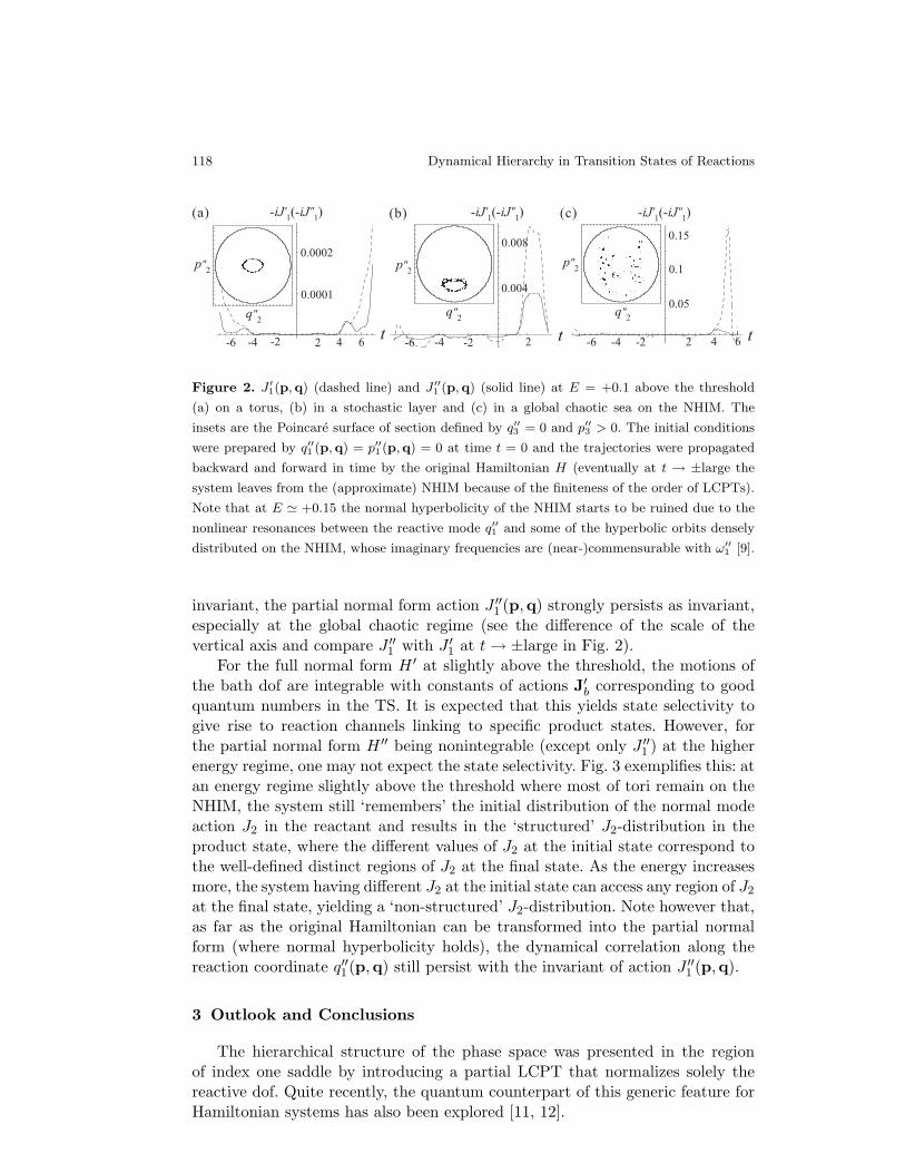
118 Dynamical Hierarchy in Transition States of Reactions
2-4 -2 4-6 6
0.0001
0.0002
t
(a)
p"2
q"2
-iJ'1(-iJ"
1)
2-4 -2-6
0.004
0.008
-iJ'1(-iJ"
1)
t
(b)
p"2
q"2
2-4 -2 4-6 6
0.05
0.1
0.15
t
p"2
q"2
(c) -iJ'1(-iJ"
1)
Figure 2. J ′1(p,q) (dashed line) and J ′′1 (p,q) (solid line) at E = +0.1 above the threshold
(a) on a torus, (b) in a stochastic layer and (c) in a global chaotic sea on the NHIM. The
insets are the Poincare surface of section defined by q′′3 = 0 and p′′3 > 0. The initial conditions
were prepared by q′′1 (p,q) = p′′1 (p,q) = 0 at time t = 0 and the trajectories were propagated
backward and forward in time by the original Hamiltonian H (eventually at t → ±large the
system leaves from the (approximate) NHIM because of the finiteness of the order of LCPTs).
Note that at E ' +0.15 the normal hyperbolicity of the NHIM starts to be ruined due to the
nonlinear resonances between the reactive mode q′′1 and some of the hyperbolic orbits densely
distributed on the NHIM, whose imaginary frequencies are (near-)commensurable with ω′′1 [9].
invariant, the partial normal form action J ′′1 (p,q) strongly persists as invariant,especially at the global chaotic regime (see the difference of the scale of thevertical axis and compare J ′′1 with J ′1 at t → ±large in Fig. 2).
For the full normal form H ′ at slightly above the threshold, the motions ofthe bath dof are integrable with constants of actions J′b corresponding to goodquantum numbers in the TS. It is expected that this yields state selectivity togive rise to reaction channels linking to specific product states. However, forthe partial normal form H ′′ being nonintegrable (except only J ′′1 ) at the higherenergy regime, one may not expect the state selectivity. Fig. 3 exemplifies this: atan energy regime slightly above the threshold where most of tori remain on theNHIM, the system still ‘remembers’ the initial distribution of the normal modeaction J2 in the reactant and results in the ‘structured’ J2-distribution in theproduct state, where the different values of J2 at the initial state correspond tothe well-defined distinct regions of J2 at the final state. As the energy increasesmore, the system having different J2 at the initial state can access any region of J2
at the final state, yielding a ‘non-structured’ J2-distribution. Note however that,as far as the original Hamiltonian can be transformed into the partial normalform (where normal hyperbolicity holds), the dynamical correlation along thereaction coordinate q′′1(p,q) still persist with the invariant of action J ′′1 (p,q).
3 Outlook and Conclusions
The hierarchical structure of the phase space was presented in the regionof index one saddle by introducing a partial LCPT that normalizes solely thereactive dof. Quite recently, the quantum counterpart of this generic feature forHamiltonian systems has also been explored [11, 12].

C.B. Li et al. 119
-0.4
J2
Pp"2
0 0.2-0.2
0
0.2
-0.2
q"2
0.040.02
(a)p"2
0 0.4-0.4
0
0.4
-0.4
q"2
J2
P
0.20.1
(b)
Figure 3. The product distribution of the normal mode action J2 at E = +0.025 (a) and
+0.1 (b) above the threshold. The initial conditions are prepared as follows: we turned off the
coupling among the modes in the reactant by putting α1 = ∞ in Eq. (5) in order to prepare
a well-defined initial condition in the reactant state. At q1 = −14.142, we fixed p1 to confirm
the crossings to the product. Then, we set an initial distribution of the action J2 such that
Pini(J2) =P3
i=1 δ(J2 − J2i) with three initial values of J2 indicated by three arrows (J3 is
automatically determined with the fixed J1 and J2 at a given E) with the uniform sampling
for the angle variable θ2 (and θ3). Then, the ensemble of trajectories of the initial conditions
were evolved using the original Hamiltonian until they reach the product at q1 = 14.142. The
inset are the Poincare surface of section defined by q′′3 = 0 and p′′3 > 0 on the NHIM (See the
figure caption of Fig. 2 in detail).
Acknowledgement. Parts of this work were supported by JSPS, Grant-in-Aid for Research onPriority Area ‘Control of Molecules in Intense Laser Fields’ of the Ministry of Education,Science, Sports and Culture of Japan, Japan Science and Technology and 21st century COE(Center Of Excellence) of ‘Origin and Evolution of Planetary Systems (Kobe Univ.)’, MEXT.
References
1. Toda, M. et al. (eds.): Adv. Chem. Phys. 130 (2005) and references therein.2. Komatsuzaki, T., Berry, R. S.: J. Chem. Phys. 110, 9160 (1999); Phys. Chem. Chem.
Phys. 1, 1387 (1999); Proc. Natl. Acad. Sci. USA 78, 7666 (2001); J. Chem. Phys.115, 4105 (2001); J. Chem. Phys. 116, 862 (2002); J. Phys. Chem. A 106, 10945(2002); Adv. Chem. Phys. 123, 79 (2002); Adv. Chem. Phys. 130A, 143 (2005)
3. Toda, M.: Phys. Rev. Lett. 74, 2670 (1995); Phys. Lett. A 227, 232 (1997); Adv.Chem. Phys. 123, 153 (2002); Adv. Chem. Phys. 130A, 337 (2005)
4. Koon, W.S. et al.: Chaos 10, 427 (2000)5. Wiggins, S. et al.: Phys. Rev. Lett. 86, 5478 (2001)6. Uzer, T. et al.: Nonlinearity 15, 957 (2002)7. Waalkens, H. et al.: J. Chem. Phys. 121, 6207 (2004)8. Li, C.B. et al.: J. Chem. Phys. 123, 184301 (2005)9. Li, C.B. et al.: (unpublished)
10. Moser, J.: Comm. Pure Appl. Math. 11, 257 (1958)11. Creagh, S.C.: Nonlinearity 17, 1261 (2004); Nonlinearity 18, 2089 (2005)12. Cargo, M. et al.: J. Phys. A 38, 1977 (2005)

Few-Body Systems 0, 121–126 (2006) Few-Body
Systemsc© by Springer-Verlag 2006
Printed in Austria
Fractal Structure in Ionization Dynamics∗
J. B. Delos 1, K. A. Mitchell2
1 Department of Physics, College of William and Mary, Williamsburg, Virginia, 23187-87952 School of Natural Sciences, University of California, Merced, California, 95344
Abstract. Chaotic dynamics in open systems produces fractals. This can beseen, for example, in the ionization of an electron from a hydrogen atom inapplied parallel electric and magnetic fields. We summarize some of our recentwork on the order that can be found in these fractals.
We discuss here a prediction for a proposed experiment which has not yetbeen performed: the ionization of hydrogen by a short laser pulse
H + hν → H∗ → H+ + e− (1)
in parallel electric and magnetic fields. We predict that electrons will arrive at adetector in a train of pulses (Fig. 1a). This pulse train results from fractal struc-ture in the dynamics, what we call an “epistrophic fractal.” As is well known, afractal is a geometric set typically with some kind of repeating self-similar struc-ture within structure. “Epistrophe” is a term from rhetoric, meaning a regularending following variable beginnings. Thus, an epistrophic fractal is a class ofa fractal in which there are variable beginnings and self-similar endings at alllevels of resolution.
For a selection of work on the dynamics of transport and escape that hasbeen influential to our own studies, please see the work by Tiyapan and Jaffe [1],Easton [2], Rom-Kedar [3], Jung and coworkers [4], and Collins [5]. See alsorecent work on the phase space formulation of transition states [6].
Pulse trains in the decay of excited atoms have been previously observedby Lankhuijzen and Noordam [7]. Measuring the decay of an excited rubidiumatom in an electric field with picosecond time resolution, they found that thedecay is not exponential, but instead occurs in a sequence of pulses; the timeinterval between pulses is approximately equal to the return time of an electrontrajectory to the atomic core.
We consider an analogous experimental setup to that of Lankhuijzen andNoordam, but using hydrogen in parallel electric and magnetic fields. We de-scribe the electron’s motion purely by classical mechanics. Effects of quantummechanics on the electron’s motion will be examined in future studies.∗Article based on the presentation by J. B. Delos at the Fourth Workshop on the Dynamicsand Structure of Critically Stable Quantum Few-Body Systems, MPIPKS, Dresden, Germany,2005. Received December 6, 2005; Accepted December 9, 2006

122 Fractal Structure in Ionization Dynamics
Time T (scaled units)
Ioni
zatio
n ra
te (
arb.
uni
ts)
2 3 4 5 6 7 8 9
0
0.05
0.1
0.15
2 3 4 5 6 7 8 9
1.8
1.9
2
2.1
2.2
2.3
θ
Time T (scaled units)01234567
1.8
1.9
2
2.1
2.2
2.3
Iterate at escape
θ
01234567
1.8
1.9
2
2.1
2.2
2.3
Iterate at escape
θ
(a)
(b) (c)
(d)
*Direct
A1
*B1
C1A2A3
A1
B1 B2
C1C2
A3
B1*
A4
C2
B2
C1
A2
A1
Direct
Direct
Figure 1. (a) For hydrogen in parallel fields, the flux of electrons striking a detector is plotted
vs. time T . The thin line is a model assuming ∆E = ∆T = 0, whereas the thick line assumes
a minimum uncertainty wavepacket, with central energy E = −1/(2 × 802) and ∆T = 5.2ps.
We use magnetic field B = 0.49T, electric field F = 19V/cm, and one scaled unit of time T
equal to 52ps. (b) Time to strike the detector plotted vs. the initial launch angle θ. The dashed
lines connect icicles to their corresponding pulses. (c) The number of iterates to escape the
complex vs. launch angle θ. Each escape segment corresponds to an icicle. (d) The dashed lines
connect segments within one epistrophe. The solid arrows show the creation of new epistrophes
according to the Epistrophe Start Rule. The asterisk denotes a “strophe” segment.
The time for an electron to ionize is a sensitive function of its initial launchangle from the atom. A graph of escape time T vs. initial angle θ is shownin Fig. 1b. If the electron initially moves away from the atom in the “downhill”direction (i.e. in the direction of the electric force), then it escapes from the atomquickly. If it leaves in the “uphill” direction, it never escapes. At intermediateangles there is a very complex behavior, with structure-within-structure at alllevels of resolution. This “escape-time plot” governs the structure of the pulsetrain: the probability current of electrons arriving at a detector is proportionalto the derivative dθ/dT of the escape-time plot, so each “icicle” in the escapetime plot produces a pulse of electrons arriving at the detector.
The escape-time plot is simplified by use of a Poincare surface of section(SOS) and corresponding Poincare return map. Every time the electron crossesthe negative z-axis, we record the value of (z, pz). (We transform the (z, pz)coordinates to a “smoother” set of coordinates (q, p) used in Fig. 2.) The SOScontains an unstable fixed point zX (Fig. 2), which corresponds to an unstable

J. B. Delos and K. A. Mitchell 123
−1.5 −1 −0.5 0 0.5 1−1.5
−1
−0.5
0
0.5
1
1.5
q
pP0
Q0
Q1zX
E1E0E1
E2
C0C1C1
L0S
UComplex
Figure 2. A surface-of-section plot showing the unstable fixed point zX with its homoclinic
tangle of intersecting stable (S) and unstable (U) manifolds.
periodic orbit that forms a Periodic Orbit Dividing Surface (PODS). (In orderfor the electron to escape, it must pass over the PODS in configuration space.)The fixed point zX has stable and unstable manifolds, S and U , which intersect ina complicated pattern called a “homoclinic tangle”. Choosing a particular inter-section point P0, the segments of S and U that connect zX to P0 define a regionof the Poincare plane, which we call the “complex”. The complex represents thatpart of phase space in which the electron has enough energy to escape but is stilloscillating chaotically around the nucleus. The electron trajectories begin nearthe nucleus and move radially outward in all directions. The initial ensemble ofelectrons forms a line of initial conditions L0 in the SOS.
The Poincare map provides a second way of measuring how long the electrontakes to escape: we count the number of iterates of the map required beforethe phase point leaves the complex. This measure of escape time “rectifies” thecontinuous escape-time plot (Fig. 1b) into discrete escape segments (Fig. 1c).
In Fig. 1b, 1c, or 1d, we can see the first few segments from several infiniteregular sequences of escape segments, which we call “epistrophes”. In previouswork, we proved that an epistrophe converges upon each end of every escapesegment; the epistrophes are all asymptotically self-similar, and all asymptoti-cally similar to each other; they differ from one another asymptotically only byan overall scale factor; successive segments in an epistrophe decrease geometri-cally by a factor equal to the Liapunov factor of the unstable fixed point. Thus,epistrophes occur at all levels of resolution.
However, there are also other escape segments that do not fit into the regularepistrophe sequences. Numerical evidence indicates that such “surprises” mayappear at all levels of resolution, so they tend to break the self-similarity of theescape time plot.
The purpose of this research is to explain the structure of these escape-time

124 Fractal Structure in Ionization Dynamics
plots, and thereby to explain the structure that may be observed in a pulse train.We have developed a technique using algebraic topology to explain and describethese structures. We do not have sufficient space here to describe the methodin detail, but we can show how it is applied, and what kind of results it gives.The algebraic technique predicts a minimal set of topologically required escapesegments at each iterate, by the following method.
1. Compute the stable and unstable manifolds from zX to P0, i.e. computethe boundary of the complex.
2. Map the unstable manifold forward a chosen number of iterates J . Thenumber of iterates chosen determines the amount of information about thehomoclinic tangle that is used as input into the algebraic formalism, andthereby it determines the amount of information about the escape-timeplot that can be predicted.
3. Visually extract essential information about the structure of the homoclinictangle at iterate J .
4. Assign letter names to certain segments of the unstable manifold. Examplesof letter names we use are cn for 1 ≤ n ≤ D and um for 0 ≤ m < ∞. D isa finite integer called the “minimum delay time” of the complex.
5. Represent the topological structure of the line of initial conditions L0 bya word, i.e. a sequence of letters, `0. In an idealized case, we might have`0 = c1.
6. Express the action of the map in terms of symbolic dynamics on theseletters. For example, we might find um 7→ um+1, cn 7→ cn+1, cD 7→(c1c2...cD)−1u−1
0 c1c2...cD.
7. Apply this symbolic dynamics some number of iterates K to the string `0.For example, if `0 = c1, D = 1, and c1 7→ c−1
1 u−10 c1, we may iterate three
times to obtain `3 = c−11 u0c1u1c
−11 u−1
0 c1u2c−11 u0c1u
−11 c−1
1 u−10 c1. This is not
a meaningless string of letters, as we see in the next step.
8. In the string for `K , read off the structure of the minimal topologicallyrequired set of escape segments up to iterate K: for example, each factorui in `K represents a segment that escapes at iterate K − i. In the aboveexample, we obtain the following escape time plot:
321
On the first iterate, there must be one escape segment; on the second, theremust be two, one on either side of the first; and on the third, there mustbe four segments, interleaved with the preceding ones.

J. B. Delos and K. A. Mitchell 125
The algebraic computation that explains the escape time plot in Fig. 1dfollows a similar line as the example above. However, there is an additionalsequence (A1, A2, ...), which is discussed in [8], and there is another additionalescape segment, marked with an asterisk. The latter segment, which we calla “strophe”, is not predicted by topological means – we simply compute thePoincare map to the fifth iterate, at which point it appears in the numerics.However, once this segment is known to be present, one can expand the algebraicprocedure, and then compute a revised minimal set of escape segments. This newminimal set will include additional segments that are forced by the “strophe”segment at iterate five.
The details of this theory are developed in Refs. [8, 9] and [10]. The samekind of theory should be useful for describing chaotic transport in many othersystems, including atoms in other field configurations, molecular collisions, therestricted gravitational three-body problem, microwave cavities, etc.
References
1. A. Tiyapan and C. Jaffe, J. Chem. Phys. 99, 2765 (1993); 101, 10393 (1994);103, 5499 (1995).
2. R. W. Easton, Trans. Am. Math. Soc. 294, 719 (1986); Geometric Methodsfor Discrete Dynamical Systems (Oxford, New York, 1998).
3. V. Rom-Kedar, Physica D 43, 229 (1990); Nonlinearity 7, 441 (1994).
4. C. Jung and H. J. Scholz, J. Phys. A 20, 3607 (1987); B. Ruckerl and C.Jung, J. Phys. A 27, 55 (1994); B. Ruckerl and C. Jung, J. Phys. A 27,6741 (1994); C. Lipp and C. Jung, J. Phys. A 28, 6887 (1995); C. Jung,C. Lipp, and T. H. Seligman, Ann. Phys. 275, 151 (1999); T. Butikofer,C. Jung, and T. H. Seligman, Phys. Lett. A 265, 76 (2000); C. Jung andA. Emmanouilidou, Chaos 15, 023101 (2005).
5. P. Collins, in Geometry and Topology in Dynamics, edited by M. Bargeand K. Kuperberg (American Mathematical Society, Providence, 1999);P. Collins, Internat. J. Bifur. Chaos Appl. Sci. Engrg. 12, 605 (2002);P. Collins, Dyn. Syst. 19, 1 (2004); P. Collins, Dyn. Syst., to appear;P. Collins, Experiment. Math., to appear; P. Collins and B. Krauskopf, Phys.Rev. E 66, 056201 (2002).
6. W. S. Koon, M. W. Lo, J. E. Marsden, and S. D. Ross, Chaos 10, 427 (2000);T. Komatsuzaki and R. S. Berry, Proc. Nat. Acad. Sci., 98, 7666 (2001);C. Jaffe, S. D. Ross, M. W. Lo, J. Marsden, D. Farrelly, T. Uzer, Phys.Rev. Lett. 89, 011101 (2002); T. Uzer, C. Jaffe, J. Palacian, P. Yanguas,and S. Wiggins, Nonlinearity 15, 957 (2002); F. Gabern, W.S. Koon, J.E.Marsden, and S.D. Ross, Physica D (to appear).
7. G. M. Lankhuijzen and L. D. Noordam, Phys. Rev. Lett. 76, 1784 (1996);Opt. Commun. 129, 361 (1996).

126 Fractal Structure in Ionization Dynamics
8. K. A. Mitchell, J. P. Handley, B. Tighe, A. Flower, and J. B. Delos, Phys.Rev. Lett. 92, 073001 (2004); Phys. Rev. A 70, 043407 (2004).
9. K. A. Mitchell, J. P. Handley, B. Tighe, S. K. Knudson, and J. B. Delos,Chaos 13, 880 (2003); K. A. Mitchell, J. P. Handley, S. K. Knudson, andJ. B. Delos, Chaos 13, 892 (2003).
10. K. A. Mitchell and J. B. Delos, submitted to Physica D;http://faculty.ucmerced.edu/kmitchell/publications/bridges.pdf.

Few-Body Systems 0, 127–131 (2006) Few-Body
Systemsc© by Springer-Verlag 2006
Printed in Austria
Dependence of the H2–H2 interaction on the
monomer bond lengths: steps toward an
accurate ab initio estimate∗
Robert J. Hinde∗∗
Department of Chemistry, University of Tennessee, Knoxville TN 37996, USA
Abstract. We compute the vibrational coupling between two H2 moleculesfrom ab initio quantum chemical calculations of the H2–H2 potential carriedout at the full configuration interaction level of theory using the atom-centeredaug-cc-pVTZ basis set for hydrogen. We compare the full configuration inter-action results with those obtained using two variants of coupled cluster theoryand find that a fully iterative treatment of connected triples may be requiredto estimate the H2–H2 vibrational coupling accurately using coupled clustertheory.
1 Introduction
Tejeda et al. [1] have recently shown that small clusters of j = 0 H2, or parahy-drogen, molecules are formed when gaseous parahydrogen (pH2) is cooled in afree jet expansion. They demonstrate the presence of these clusters in the cooledjet by observing the clusters’ Raman-active vibrational excitations that correlatewith the pure vibrational Q1(0) transition of a single pH2 molecule. The Ramanfeatures associated with clusters of n = 2 to 7 pH2 molecules are narrow, isolated,and red-shifted from the free molecule’s Q1(0) transition at ν = 4161.18 cm−1;the red shift, which arises from weak pH2–pH2 intermolecular interactions inthe (pH2)n cluster, increases monotonically (but not linearly) with n in this sizerange.
The vibrationally excited states of the (pH2)n clusters accessed via theseRaman-active transitions are ones in which the vibrational excitation is delocal-ized over the n molecules in the cluster, and these states are thus finite-size ana-logues of the delocalized vibron states of crystalline solid H2 probed via Raman
∗Article based on the presentation by R.J. Hinde at the Fourth Workshop on the Dynamicsand Structure of Critically Stable Quantum Few-Body Systems, MPIPKS, Dresden, Germany,2005, Received November 21, 2005; Accepted December 14, 2006
∗∗E-mail address: [email protected]

128 Dependence of the H2–H2 interaction on the monomer bond lengths
r1
r2
r1
r2
r1
r2
T-shaped parallel linear
R
Figure 1. Three representative configurations of the H2–H2 dimer. The H2–H2 center of mass
distance is denoted R, while r1 and r2 represent the H2 monomer bond lengths.
spectroscopy of the bulk solid [2]. A better understanding of these delocalizedvibrational states of (pH2)n clusters could therefore shed light on the clusters’internal structures and on the question of whether the clusters exhibit signs ofsuperfluidity, as has been suggested by path integral Monte Carlo simulations [3].
The delocalization of the vibrational excitation among a cluster’s constituentmolecules is governed by terms in the H2–H2 potential energy surface that couplethe vibrational coordinates of the two pH2 molecules. At H2–H2 intermoleculardistances characteristic of the (pH2)n clusters, these terms are fairly small inmagnitude. Estimating these terms from ab initio quantum chemical calculationsthus requires the use of computational methods that have accuracy much higherthan the oft-quoted “chemical accuracy” of 1 kcal/mol. Here we investigate thesensitivity of these coupling terms to the treatment of electron correlation effectsin the underlying ab initio computations.
2 Ab initio calculations
The pH2–pH2 interaction is obtained by rotationally averaging the H2–H2 po-tential energy surface over the angular degrees of freedom of the H2 monomers.We do not perform this full rotational averaging here, but simply consider threerepresentative coplanar, high-symmetry configurations of the H2 dimer, shownin Fig. 1. For each of these configurations, we hold the H2–H2 center-of-massdistance R fixed and vary the monomer bond lengths r1 and r2. We consider twoR values: R = 3.05 A, which is close to the root (V = 0) of the potential fora (pH2)2 dimer of two v = 0 molecules, and R = 3.4 A, which is close to theminimum energy, equilibrium distance of the (pH2)2 dimer [4].
For these high-symmetry configurations, full configuration interaction (CI)calculations of the dimer’s electronic energy are feasible even for fairly large one-electron basis sets. Full CI calculations give the exact total electronic energyof the dimer for a given one-electron basis set and thus provide a referencepoint for benchmarking other electronic structure methods. We perform full CIcalculations for the H2–H2 dimer using a determinant-based algorithm [5] asimplemented in the November 22, 2004 (R1) version of the electronic structure

R.J. Hinde 129
-65-60-55-50-45-40-35-30-25-20-15-10
0.8 1 1.2 1.4 1.6 1.8 2
VF
CI (
cm-1
)
r (a0)
(a)
0
0.5
1
1.5
2
2.5
3
3.5
4
0.8 1 1.2 1.4 1.6 1.8 2
∆V
(cm
-1)
r (a0)
(b)
Figure 2. Interaction energies for T-shaped H2–H2 with monomer bond lengths r1 = r2 = r
and H2–H2 distance R = 3.4 A. (a) Full CI interaction energy VFCI. (b) Interaction energy
differences VCCSDT − VFCI (open circles) and VCCSD(T) − VFCI (filled boxes).
code GAMESS [6]. We then correct these H2–H2 total energy calculations forbasis set superposition error by applying the standard counterpoise correction [7],thereby obtaining ab initio estimates of the H2–H2 interaction energy.
We also compute the H2–H2 interaction energy for these dimer configurationsusing two variants of coupled cluster theory [8, 9], one that includes single anddouble excitations and a perturbative treatment of triple excitations [10], ab-breviated CCSD(T), and one that includes single, double, and triple excitationsin a fully iterative manner [11, 12], abbreviated CCSDT. These calculations areperformed using the tensor contraction engine [13] incorporated into version 4.7of the electronic structure code NWChem [14]. We denote these two potentialenergy surfaces as VCCSD(T) and VCCSDT respectively.
All of our ab initio calculations are performed using the atom-centered aug-cc-pVTZ basis set for hydrogen [15, 16]. To avoid convergence difficulties arisingfrom near linear dependence of the one-electron basis set at small r1 and r2 values,eigenvectors of the one-electron overlap matrix with eigenvalues below 10−6 areeliminated from the one-electron basis set for each H2–H2 configuration.
3 Results and discussion
Figure 2 shows, for T-shaped H2–H2 configurations with R = 3.4 A and monomerbond lengths r1 = r2 = r, both the full CI interaction energy VFCI and thedifferences ∆V between VFCI and either VCCSD(T) or VCCSDT. As r increases, theCCSD(T) potential begins to deviate substantially from the full CI potential,with the difference ∆V = VCCSD(T) − VFCI reaching 3.75 cm−1 (or 6% of themagnitude of VFCI) at r = 2.0 a0. By comparison, the difference between theCCSDT potential and the full CI potential remains below 0.85 cm−1 for theentire range of H2 bond lengths shown in Fig. 2.
Of particular interest are the shapes, near the equilibrium bond length req =1.4 a0, of the energy difference curves shown in Fig. 2(b). The coupling betweenthe vibrational coordinates of two H2 molecules, which leads to delocalization of

130 Dependence of the H2–H2 interaction on the monomer bond lengths
Table 1. Off-diagonal vibrational coupling matrix elements 〈V (r1, r2)〉01,10 (in cm−1) for H2–
H2 dimers.
Configuration R (A) full CI CCSDT CCSD(T)
T-shaped 3.05 −0.740 −0.718 −0.674T-shaped 3.4 −0.580 −0.566 −0.542parallel 3.05 0.572 0.576 0.595parallel 3.4 0.202 0.204 0.215linear 3.05 0.937 0.944 1.076linear 3.4 0.443 0.446 0.513
a vibrational excitation among the constituent molecules of a (pH2)n cluster, isdetermined by the derivatives of the H2–H2 potential V (r1, r2) with respect tothe monomer bond lengths r1 and r2 in the vicinity of r1 = req and r2 = req.Inspection of Fig. 2(b) suggests that the relevant derivatives of the CCSD(T)potential surface may differ significantly from those computed at the full CI levelof theory, and that a potential surface computed using the CCSD(T) method maythus give poor estimates of the degree of H2–H2 vibrational coupling in (pH2)n
clusters.To assess this quantitatively, we compute the off-diagonal vibrational cou-
pling matrix element
〈V (r1, r2)〉01,10 = 〈v1 = 0, v2 = 1|V (r1, r2)|v1 = 1, v2 = 0〉 (1)
at the full CI, CCSDT, and CCSD(T) levels of theory for the three H2–H2
configurations shown in Fig. 1. We do this by computing V (r1, r2) at 25 (r1, r2)pairs, in which r1 and r2 vary between 0.8 a0 and 2.0 a0 in 0.3 a0 steps. We thenfit these points using the function
V (r1, r2) =2∑
k=0
2∑n=0
ck,n(r1 − req)k(r2 − req)n (2)
and integrate the fit over the relevant j = 0 vibrational wavefunctions of thetwo monomers to obtain the matrix element defined in Eq. (1). Table 1 givesour results, and shows that the CCSD(T) matrix elements differ from thosecomputed at the full CI level by as much as 15% in some cases. The CCSDTmatrix elements are in much better agreement with the full CI results. Thesefindings suggest that fairly high-level ab initio methods are needed to provideinsight into the dependence of the H2–H2 potential on the vibrational states ofthe two H2 monomers.
Acknowledgement. Financial support was provided by the U.S. National Science Foundationthrough grant CHE-0414705.

R.J. Hinde 131
References
1. G. Tejeda, J. M. Fernandez, S. Montero, D. Blume, and J. P. Toennies, Phys. Rev.Lett. 92, 223401 (2004).
2. J. van Kranendonk and G. Karl, Rev. Mod. Phys. 40, 531 (1968).
3. P. Sindzingre, D. M. Ceperley, and M. L. Klein, Phys. Rev. Lett. 67, 1871 (1991).
4. J. Schaefer and W. E. Kohler, Z. Phys. D 13, 217 (1989).
5. P. J. Knowles and N. C. Handy, Chem. Phys. Lett. 111, 315 (1984).
6. M. W. Schmidt, K. K. Baldridge, J. A. Boatz, S. T. Elbert, M. S. Gordon, J. H.Jensen, S. Koseki, N. Matsunaga, K. A. Nguyen, S. Su, T. L. Windus, M. Dupuis,and J. A. Montgomery, J. Comput. Chem. 14, 1347 (1993).
7. S. F. Boys and F. Bernardi, Mol. Phys. 19, 553 (1970).
8. J. Cizek, J. Chem. Phys. 45, 4256 (1966).
9. R. J. Bartlett, J. Phys. Chem. 93, 1697 (1989).
10. K. Raghavachari, G. W. Trucks, J. A. Pople, and M. Head-Gordon, Chem. Phys.Lett. 157, 479 (1989).
11. J. Noga and R. J. Bartlett, J. Chem. Phys. 86, 7041 (1987).
12. J. Noga and R. J. Bartlett, J. Chem. Phys. 89, 3401 (1988).
13. S. Hirata, J. Phys. Chem. A 107, 9887 (2003).
14. E. Apra et al., “NWChem: A computational chemistry package for parallel comput-ers” available from 〈http://www.emsl.pnl.gov/docs/nwchem/nwchem.html〉 (2005).
15. T. H. Dunning, Jr., J. Chem. Phys. 90, 1007 (1989).
16. D. E. Woon and T. H. Dunning, Jr., J. Chem. Phys. 100, 2975 (1994).
Few-Body Systems 0, 132–137 (2006) Few-Body
Systemsc© by Springer-Verlag 2006
Printed in Austria
Resonances in muon transfer from muonic
hydrogen to oxygen and neon∗
Timur V. Tscherbul∗∗, Bruno Lepetit ∗∗∗, Arnaud Dupays
Laboratoire Collisions, Agregats, Reactivite (UMR 5589 CNRS-UPS), IRSAMC, UniversitePaul Sabatier Toulouse 3, 31062 Toulouse cedex 9, France
Abstract. The influence of resonances on the muon transfer processes frommuonic hydrogen to oxygen and neon : (pµ)1s + O8+ → p + µ(O)7+nl and(pµ)1s + Ne10+ → p + µ(Ne)9+
nl is considered using Smith lifetime matrixformalism. It is shown that the existence of a long lived resonance in the caseon Ne induces a stronger dependence on collision energy of the muon transfercross-section for this system.
1 Introduction
High precision muonic hydrogen spectroscopy provides detailed information onthe predictions of quantum electrodynamics and on the electromagnetic structureof the proton [1]. One example is the measurement of hyperfine structure ofground 1s muonic hydrogen, from which one can expect improved knowledge onthe Zeemach radius of the proton [4]. Muon transfer reactions involving elementsXZ+ with high atomic charges Z (for instance O or Ne)
(pµ)1s + XZ+ → p + µ(X)(Z−1)+nl (1)
can be used to probe muonic hydrogen population in such spectroscopic studies.Indeed, the product complex of the charge exchange µ(X)(Z−1)+
nl is formed in anexcited state and relaxes through emission of X rays which can be easily detected.
As an example, a measurement of the hyperfine structure of ground muonichydrogen (pµ)1s using charge transfer to oxygen has been proposed recently [6].In this experiment, a tunable laser source is used to populate the excited hyper-fine level of thermal (pµ)1s. This excited state relaxes quickly to the ground levelthrough collisions with surrounding hydrogen, but keeps a significant fraction of∗Article based on the presentation by B. Lepetit at the Fourth Workshop on the Dynamicsand Structure of Critically Stable Quantum Few-Body Systems, MPIPKS, Dresden, Germany,2005. Received November 10, 2005; Accepted November 22, 2005
∗∗Present address: Department of Chemistry, Moscow State University, Moscow 119992 Russia∗∗∗E-mail address:[email protected]

T.V. Tscherbul, B. Lepetit, A. Dupays 133
the energy brought in by the laser in kinetic energy, thus yielding hyperthermalmuonic hydrogen. If the muon transfer process depends significantly on collisionenergy, then formation of hyperthermal hydrogen will impact the intensity ofthe emitted X ray. Measurement of the emitted intensity as a function of thelaser frequency thus provides information of the relative hyperthermal and ther-mal hydrogen populations and allows an indirect measurement of the hyperfinesplitting. Oxygen was originally proposed as highly charged colliding partner be-cause of experimental evidence that muon exchange rate may depend stronglyon kinetic energy in that case [7].
Recently, muon transfers to different high charge elements have been studiedtheoretically by several groups using different methods : hyperspherical coordi-nates [2, 3, 5, 8], entrance channel Jacobi coordinates [9] or semiclassical meth-ods [10]. Hyperspherical coordinate studies suggested that the dependence of thetransfer rate on collision energy may be even larger for neon than for oxygen. Inparticular, it has been suggested that metastable states in the entrance channelof the collision can have a prominent effect on the dependence of J-resolved in-tegral cross sections on collision energy, where J is the total angular momentumquantum number. The purpose of the present paper is to examine the presenceand manifestation of these resonances in more details using Smith [11] lifetimeQ-matrix formalism.
2 Method
Time-independent close-coupling calculations on the charge exchange processes(1) are performed using hyperspherical elliptic coordinates [14, 15]. One promi-nent advantage of these coordinates is to transform the coulomb potential intoa regularized one which is approximately separable. The total wavefunction isexpanded for O and Ne on a basis of respectively 88 and 133 channel functionsobtained by diagonalizing a fixed hyperradius hamiltonian. The channel func-tions in turn are expanded on products of Wigner functions for the Euler angles,and products of 150 one dimensional basis functions for the two internal hyper-angles. Dependence on the hyperradius of the total wavefunction and scatteringS-matrices are obtained for each collision energy by integrating a set of coupleddifferential equations from a small value of the hyperradius up to the asymtoticregion (typically, 1 A). Cross sections are obtained by summation over the totalangular momentum J up to J = 4. Details on this method can be found in Ref.[4].
The Smith [11] lifetime Q-matrix is defined as :
Q = i~S(
dSdE
)†, (2)
where S is the scattering matrix and E is the collision energy. The eigenvaluesof Q correspond to the lifetimes of metastable states [11]. In the vicinity of anisolated narrow resonance, the maximum eigenvalue qmax has a Lorentzian shapeas a function of E which gives the energy Er and width Γ of the resonance. Thisprovides with a practical tool to characterize resonances.

134 Muon transfer
102
103
104
Cro
ss s
ectio
n / [
m. u
.]2
J = 0J = 1J = 2J = 3J = 4
0,001 0,01 0,1 1 10Collision energy / eV
10-5
10-4
10-3
10-2
10-1
Eig
enlif
e-tim
e / p
icos
econ
dsO + pµ -> p + (Oµ)
Figure 1: Maximum eigenvalue of the lifetime matrix (2) in picoseconds for thereaction (pµ)1s + O8+ → p + µ(O)7+
nl for several J values (lower panel), and thecorresponding integral cross sections (upper panel) in muonic units (1/mµ ≈1/207 Bohr, where mµ stands for the mass of muon with respect to the one ofthe electron) as functions of collision energy.
The lifetime matrix (2) is computed by use of a three-point central finitedifference method. The energy-dependent stepsize for derivative evaluation istaken to be 10−2 × E which ensures the convergence of the eigenlife-time qmax
better that 1 %. We have checked the deviations from hermiticity of our numericalQ-matrix and found them to be negligible in the energy region considered in thiswork.
3 Results
In figure 1, J-resolved muon transfer cross sections and lifetimes are presented forthe process (1). At low energy, the cross-section is given by the Wigner thresholdlaw [12] and depends on collision energy as EJ−1/2. As a result, the J = 0 cross-section diverges at zero collision energy, and the J 6= 0 cross-sections increaselinearly on figure 1 (in log-scale) with energy. Wigner threshold law is valid aslong as the De Broglie wavelength of the colliding partners is large compared to
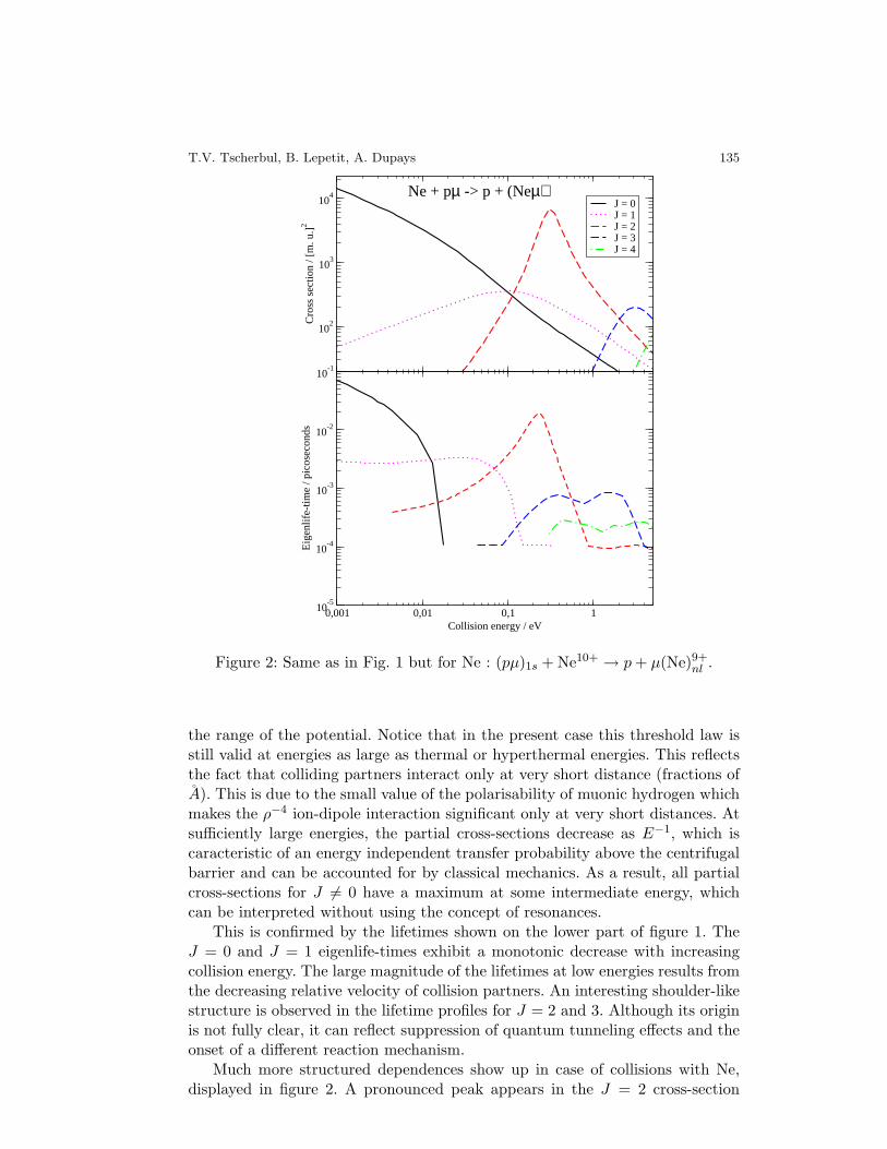
T.V. Tscherbul, B. Lepetit, A. Dupays 135
102
103
104
Cro
ss s
ectio
n / [
m. u
.]2
J = 0J = 1J = 2J = 3J = 4
0,001 0,01 0,1 1Collision energy / eV
10-5
10-4
10-3
10-2
10-1
Eig
enlif
e-tim
e / p
icos
econ
ds
Ne + pµ -> p + (Neµ)
Figure 2: Same as in Fig. 1 but for Ne : (pµ)1s + Ne10+ → p + µ(Ne)9+nl .
the range of the potential. Notice that in the present case this threshold law isstill valid at energies as large as thermal or hyperthermal energies. This reflectsthe fact that colliding partners interact only at very short distance (fractions ofA). This is due to the small value of the polarisability of muonic hydrogen whichmakes the ρ−4 ion-dipole interaction significant only at very short distances. Atsufficiently large energies, the partial cross-sections decrease as E−1, which iscaracteristic of an energy independent transfer probability above the centrifugalbarrier and can be accounted for by classical mechanics. As a result, all partialcross-sections for J 6= 0 have a maximum at some intermediate energy, whichcan be interpreted without using the concept of resonances.
This is confirmed by the lifetimes shown on the lower part of figure 1. TheJ = 0 and J = 1 eigenlife-times exhibit a monotonic decrease with increasingcollision energy. The large magnitude of the lifetimes at low energies results fromthe decreasing relative velocity of collision partners. An interesting shoulder-likestructure is observed in the lifetime profiles for J = 2 and 3. Although its originis not fully clear, it can reflect suppression of quantum tunneling effects and theonset of a different reaction mechanism.
Much more structured dependences show up in case of collisions with Ne,displayed in figure 2. A pronounced peak appears in the J = 2 cross-section

136 Muon transfer
centered at E = 0.3 eV. The J = 0 cross section exhibits a behaviour similarto that of oxygen (see figure 1), and the corresponding rate constant approachessome finite value in zero energy limit.
The eigenlife-times versus collision energy for Ne are also reported in Fig. 2.The J = 0 and J = 1 eigenlifetimes decrease or remain almost constant withcollision energy, as for oxygen. A pronounced J = 2 resonance is identified atE = 0.223 eV. It corresponds to the increase of eigenlife-time by one order ofmagnitude with respect to the background and clearly affects the cross sectionalthough the corresponding peak is slightly shifted. The J = 3 and J = 4 lifetimeshave 2 peaks, the lower energy one having no physical relevance because it is ina energy range where transfer cross-sections are negligible. The higher energypeaks are located around 1.76 eV and 3.5 eV, respectively. One is tempted toattribute them to the same resonance as for J = 2, but shifted higher in energyby the centrifugal potential and more strongly coupled to the continuum.
The relationEr(J) = Er(0) + BJ(J + 1), (3)
where B is the rotational constant, provides an analysis of the J-dependence ofresonance properties (see, for example, Ref. [13] and references therein). FromEr(J = 3) = 1.759 eV and Er(J = 2) = 0.229 eV, we get the value of theJ = 0 resonance energy Er(J = 0) = −1.302 eV and the rotational constantB = 0.255 eV. The values Er(J = 0) and B are consistent with the energy of theJ = 4 resonance extracted from a very shallow maximum centered around 3.5eV, see figure 2. The rotational constant provides the value of the hyperradius〈ρ〉 associated with the geometry of the metastable state (which is assumed tobe close to linear), B = (2µ〈ρ〉2)−1, where µ is the three-body reduced mass[2, 3]. We estimate 〈ρ〉 = 0.04 A. This value is close to the minimum of thehyperspherical adiabatic curve corresponding to the entrance channel (see figure3 in ref. [3]) , where the metastable state is expected to be trapped by the J = 2centrifugal barrier.
Using again the relation (3), we obtain the energies of “hypothetical” reso-nances at J = 0 and 1 as −1.302 and −0.792 eV, respectively. This explains whyno peaks are observed in figure 2 for these partial waves. Indeed, these resonancesare below the Ne10+ · · · (pµ)1s dissociation threshold and cannot appear in themuon transfer process.
4 Conclusion
We have studied the influence of resonances on the muon transfer from muonichydrogen to oxygen and neon at thermal and hyperthermal energies. We haveshown that a prominent resonance appears for partial waves J = 2 and above inthe case of neon. For the partial waves J = 0 and 1, this resonance is below thethreshold for muon exchange and cannot show up in this process. The presenceof the resonance induces a sharp dependence of the muon transfer cross-sectionon collision energy. This suggests that neon may be a good candidate in thehyperfine splitting measurement of ground muonic hydrogen.
However, resonance characteristics are known to be sensitive to details of

T.V. Tscherbul, B. Lepetit, A. Dupays 137
the interaction. Our model neglects several aspects of the interaction which mayhave a weak, but still significant, effect on the resonance. One is the role of theelectrons of the oxygen or neon. The charge transfer takes place at interatomicdistances which are small compared to electronic orbital radii. The screeningeffect of the electrons is thus expected to be small, although core orbitals mayplay a role. Another aspect is the hyperfine interaction, which has been neglectedin the present treatment. The hyperfine splitting of muonic hydrogen, whichresults from the interaction between the muon spin and the magnetic field createdby the proton spin in the nucleus, is 0.18 eV, which is of the same order ofmagnitude as the collision energies considered here. The approach of oxygen orneon may perturb sufficiently the muon wavefunction near proton to yield asignificant effect. Work along this line is currently in progress.
Acknowledgement. T.V.T. gratefully acknowledges financial support from an INTAS YS fel-lowhip grant No 03–55–1450.
References
1. L. I. Ponomarev, Hyperfine Interact. 138, 15 (2001).
2. A. Dupays, B. Lepetit, J. A. Beswick, C. Rizzo, and D. Bakalov, Phys. Rev. A 68,062506 (2003).
3. A. Dupays, B. Lepetit, J. A. Beswick, C. Rizzo, and D. Bakalov, Phys. Rev. A 69,062501 (2004).
4. A. Dupays, J. A. Beswick, B. Lepetit,, C. Rizzo, and D. Bakalov, Phys. Rev. A 68,052503 (2003).
5. A. Dupays, Phys. Rev. Lett. 93, 043401 (2004).
6. A. Adamczak, D. Bakalov, K. Bakalova, E. Polacco and C. Rizzo, Hyperfine Interact.136, 1 (2001)
7. A. Werthmuller, A. Adamczak, R. Jacot-Guillarmod, L.S.F. Mulhauser, L. Schel-lenger, H. Schneuwly, Y. Thalmann and S. Tresch, Hyperfine Interact., 116, 1 (1998)
8. A.-T. Le and C. D. Lin Phys. Rev. A 71, 022507 (2005)
9. S.V. Romanov Eur. Phys. J. D 28, 11 (2004)
10. V.I. Savichev, R. Blumel Eur. Phys. J. D 21, 3 (2002)
11. F. T. Smith, Phys. Rev. 118, 349 (1960).
12. E. P. Wigner, Phys. Rev. 73, 1002 (1948).
13. V. Aquilanti, S. Cavalli, A. Simoni, A. Aguilar, J. M. Lucas, and D. De Fazio, J.Chem. Phys. 121, 11675 (2004).
14. O.I. Tolstikhin, S. Watanabe, and M. Matsuzawa, Phys. Rev. Lett. 74, 3573 (1995).
15. O.I. Tolstikhin, and M. Matsuzawa, Phys. Rev. A 63, 062705 (2001).

Few-Body Systems 0, 138–141 (2006) Few-Body
Systemsc© by Springer-Verlag 2006
Printed in Austria
The kinematical model of the sudden
break-up of the three-body rigid rotator∗
A.V. Meremianin∗∗
Max-Planck-Institute for the Physics of Complex Systems, 01187 Dresden, Germany, andREC-010, Voronezh State University, 394006 Voronezh, Russia
Abstract. The angular distributions of fragments resulting from the completefragmentation of a three-body rigid rotator are considered. It is shown thatthe symmetry of the initial bound state induces the symmetry of the angulardistributions. Examples of the angular distributions corresponding to differentvalues of the angular momentum of the initial state are presented using thetechnique of Dalitz plots.
We consider the complete fragmentation of a system of three neutral particlesbound by the fixed-range force. The study of such a process is motivated mainlyby the experiments [1, 2] on the predissociation of the metastable triatomichydrogen molecule H∗
3 ,
H∗3 → H(1s) + H(1s) + H(1s),
where H(1s) denotes the hydrogen atom in its ground state. We model thepredissociation process using the sudden approximation and making the followingassumptions. At some moment of time, the rigid system of three particles acquiresa strong but short kick which leads to the complete fragmentation of the system.We assume that there is no interaction between particles as soon as they leavetheir equilibrium positions. In other words, in the initial state the particles werebound by infinitely strong fixed-range forces which suddenly go to zero. This canbe denoted as a “break down” of the three-body system.
We presume that the initial state corresponds to the symmetric top rigidrotator. In order to avoid the question of the permutational symmetry we con-sider the case when all particles are distinguishable. In lowest approximation,the amplitude A of such a “break down” process is given by the overlap integral
〈Ψj,µ,ν |Ψc〉, (1)
∗Article based on the presentation by A.V. Meremianin at the Fourth Workshop on the Dy-namics and Structure of Critically Stable Quantum Few-Body Systems, MPIPKS, Dresden,Germany, 2005. Received November 10, 2005; Accepted December 8, 2005
∗∗E-mail address: [email protected]

A.V. Meremianin 139
where Ψj,µ,ν is the wave function of the initial (bound) state of the system havingwell-defined angular momentum quantum numbers j, µ, ν; Ψc is the continuumwave function of the three free particles. Thus, the continuum wave function is aproduct of plane waves, Ψc = exp[i(k1 ·R1 +k2 ·R2 +k3 ·R3)], where the vectorRi and ki are the position vector and the asymptotic linear momentum of thei-th particle. We consider the case where all particles have equal masses. Underan assumption that CM of particles is not moving, so that k1 +k2 +k3 = 0, thewave function Ψc reduces to the product of two plane waves,
Ψc = ei(q1·ρ1+q2·ρ2), (2)
where the Jacobi position ρ1,2 and momenta vectors q1,2 are defined by
ρ1 = R3 −R2, ρ2 =32(R3 + R2)−R1, q1 =
k3 − k2
2, q2 = −k1, (3)
The wave function of the initial state of the rigid rotator has the form
Ψj,µ,ν(ρ1,ρ2) = δ(ρ1 − r1)δ(ρ2 − r2)δ(θρ − θ)Djµ,ν(Ω), (4)
where Ω denotes the set of Euler angles describing the rotation of the body-frame(BF) with respect to the lab-frame (LF), j is the angular momentum quantumnumber and µ, ν are the projections of the angular momentum operator on thez-axes of BF and LF, respectively. Dirac δ-functions fix the shape of the rigidtriangle which is described by three parameters r1, r2 and θ, where θ is the anglebetween the Jacobi vectors corresponding to the rigid triangle. For the symmetrictop rigid rotator this triangle is isosceles and θ = π/2.
Now, the overlap integral (1) can be written as
Aj,µ,ν(q1,q2) = 〈Ψj,µ,ν |Ψc〉 =∫
dρ1
∫dρ2 Ψj,µ,ν(ρ1,ρ2)ei(q1·ρ1+q2·ρ2)
=∫
Djµ,ν
∗(Ω)ei(q1·ρ1r1+q2·ρ2r2) dΩ, (5)
where ρ1,2 = ρ1,2/ρ1,2. In the derivation we have used the expression for theintegration volume element dρ1 dρ2 = dξρdΩ where dξρ = sin θρdθρρ
21dρ1ρ
22dρ2
is the volume element in the shape space. The integration over dξr disappearsbecause of the δ-function in eq. (4). As is seen, the amplitude Aj,µ,ν(q1,q2), canbe interpreted as the wave function of the three-body symmetric top rigid rotatorin the momentum representation.
In order to calculate the integral (5) one has to specify explicitly the positionof the Jacobi vectors ρ1,2 with respect to the coordinate axes of the BF, as wellas the coordinates of the Jacobi momenta vectors q1,2 in the LF. These choicesare, of course, just a matter of convenience [3]. In the case of the initial P -state(j = 1) the integral (5) can be brought to the form [3],∫
ei(q1·ρ1r1+q2·ρ2r2) [ρ2 × ρ2]sin θ
dΩ = −8π[q1 × q2]
sinχ
∫ π
0
sin√
A−B cos γ√A−B cos γ
cos γ dγ,
(6)
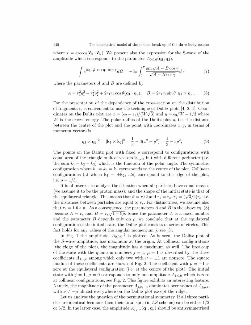
140 The kinematical model of the sudden break-up of the three-body rotator
where χ = arccos(q1 · q2). We present also the expression for the S-wave of theamplitude which corresponds to the parameter A0,0,0(q1,q2),∫
ei(q1·ρ1r1+q2·ρ2r2) dΩ = −8π
∫ π
0
sin√
A−B cos γ√A−B cos γ
dγ (7)
where the parameters A and B are defined by
A = r21q
21 + r2
2q22 + 2r1r2 cos θ(q1 · q2), B = 2r1r2 sin θ |q1 × q2|. (8)
For the presentation of the dependence of the cross-section on the distributionof fragments it is convenient to use the technique of Dalitz plots [4, 2, 1]. Coor-dinates on the Dalitz plot are x = (ε2 − ε1)/(W
√3) and y = ε3/W − 1/3 where
W is the excess energy. The polar radius of the Dalitz plot ρ, i.e. the distancebetween the centre of the plot and the point with coordinates x, y, in terms ofmomenta vectors is
|q1 × q2|2 = |k1 × k2|2 =13− 3(x2 + y2) =
13− 3ρ2, (9)
The points on the Dalitz plot with fixed ρ correspond to configurations withequal area of the triangle built of vectors k1,2,3 but with different perimeter (i.e.the sum k1 + k2 + k3) which is the function of the polar angle. The symmetricconfiguration where k1 = k2 = k3 corresponds to the centre of the plot. Collinearconfigurations (at which k1 = ±k2, etc) correspond to the edge of the plot,i.e. ρ = 1/3.
It is of interest to analyse the situation when all particles have equal masses(we assume it to be the proton mass), and the shape of the initial state is that ofthe equilateral triangle. This means that θ = π/2 and r1 = re, r2 = (
√3/2)re, i.e.
the distances between particles are equal to re. For distinctness, we assume alsothat re = 1.6 a.u.. As a consequence, the parameters A and B in the above eq. (8)become A = re and B = re
√1− 9ρ. Since the parameter A is a fixed number
and the parameter B depends only on ρ, we conclude that at the equilateralconfiguration of the initial state, the Dalitz plot consists of series of circles. Thisfact holds for any values of the angular momentum j, see [3].
In Fig. 1 the amplitude |A0,0,0|2 is plotted. As is seen, the Dalitz plot ofthe S-wave amplitude, has maximum at the origin. At collinear configurations(the ridge of the plot), the magnitude has a maximum as well. The break-upof the state with the quantum numbers j = 1, µ = 1 is described by the threecoefficients A1,1,ν among which only two with ν = ±1 are nonzero. The squaremoduli of these coefficients are shown of Fig. 2. The coefficient with µ = −1 iszero at the equilateral configuration (i.e. at the centre of the plot). The initialstate with j = 1, µ = 0 corresponds to only one amplitude A1,0,0 which is zeroat collinear configurations, see Fig. 2. This figure exhibits an interesting feature.Namely, the magnitude of the parameter Aj,µ,−µ dominates over values of Aj,µ,ν
with ν 6= −µ almost everywhere on the Dalitz plot except the ridge.Let us analyse the question of the permutational symmetry. If all three parti-
cles are identical fermions then their total spin (in LS scheme) can be either 1/2or 3/2. In the latter case, the amplitude Aj,µ,ν(q1,q2) should be antisymmetrised

A.V. Meremianin 141
0
0.0001
0.0002
0.0003
0.0004
0.0005
0.0006
0.0007
0.0008
0.0009
0.001
0 0.05 0.1 0.15 0.2 0.25 0.3
j=0 W = 5 eVW = 10 eVW = 20 eV
ρ
Figure 1. The Dalitz plot for the S-wave multipole |A0,0,0|2 corresponding to the excess energies
W = 0.5, 5, 10, 20 eV as functions of the polar radius ρ of the plot.
0
0.001
0.002
0.003
0.004
0.005
0.006
0.007
0 0.05 0.1 0.15 0.2 0.25 0.3
W = 5 eVW = 10 eVW = 20 eV
j = 1, µ = 0
ρ 0
0.0002
0.0004
0.0006
0.0008
0.001
0.0012
0.0014
0 0.05 0.1 0.15 0.2 0.25 0.3
W = 5 eV, j = 1, µ = 1 ν = −1ν = 1
ρ
0.0018
0.0016
Figure 2. The magnitudes of the parameters |A1,0,0|2 for different energies W and parameters
|A1,1,±1|2 for W = 5 eV .
with respect to the interchange of vectors q1 and q2. For the initial state hav-ing symmetry of an equilateral triangle the antisymmetrisation will give zero.In the case of the spin 1/2, the total wave function cannot be presented as asingle product of the spatial and spinor parts. Thus, the amplitude for that caseremains finite and the corresponding Dalitz plot will still consists of circles.
The “kinematical” model considered above can be generalised in order toaccount for small vibrations in the initial state. This can be done by multiply-ing the amplitude A in (5) with the vibrational wave function and subsequentintegration over the shape variables r1,2 and θ.
Acknowledgement. This work has been supported in part by CRDF and RF ministry of educa-tion in BRHE program, Grant No Y2-CP-10-02
References
1. U Muller, Th Eckert, M Braun, and H Helm. Phys. Rev. Lett., 83, pp. 2718–2721,1999.
2. U Galster, U Muller, and H Helm. Phys. Rev. Lett., 92, 073002, 2004.3. A V Meremianin. J. Phys. B: At. Mol. Opt. Phys., 38, pp. 757–775, 2005.4. R H Dalitz. Philos. Mag, 44, p. 1068, 1953.

Few-Body Systems 0, 142–145 (2006) Few-Body
Systemsc© by Springer-Verlag 2006
Printed in Austria
Scattering Length for Helium Atom-Diatom
Collision∗∗∗
E. A. Kolganova1,2, A. K. Motovilov2, and W. Sandhas3
1 Max-Planck-Institut fur Physik komplexer Systeme, Nothnitzer str. 38, 01187 Dresden, Ger-many
2 Bogoliubov Laboratory of Theoretical Physics, JINR, Joliot-Curie 6, 141980 Dubna, MoscowRegion, Russia
3 Physikalisches Institut, Universitat Bonn, Endenicher Allee 11-13, D-53115 Bonn, Germany
Abstract. We present results on the scattering lengths of 4He–4He2 and3He–4He2 collisions. We also study the consequence of varying the couplingconstant of the atom-atom interaction.
1 Introduction
The two-body scattering length in a dilute gas of alkali atoms can be varied bychanging the external magnetic field close to a Feshbach resonance [1]. In thisway one may force the two-body s-wave scattering length to go from positiveto negative values through infinity. Therefore, the magnetic field should be anappropriate tool in modeling the Efimov effect. We recall that this effect occursin case of infinite two-body scattering lengths, manifesting itself in an infinitenumber of three-body bound states.
This role of the magnetic field combined with a Feshbach resonance may bemimicked by varying the coupling constant of the two-body interaction withina three-body system that is not necessarily subject to a magnetic field [2]. Inthis context the system of three 4He atoms appears to be the best candidate.Actually, it has been shown that the excited state of the 4He trimer is alreadyof Efimov nature. To get the complete Efimov effect it suffices to weaken theHe–He interatomic potential only by about 3%.
In the present work we extend the investigation of the three-atomic heliumsystems undertaken in [3], which was based on a mathematically rigorous hard-core version of the Faddeev differential equations. We calculate the scattering∗This work was supported by the Deutsche Forschungsgemeinschaft (DFG), the Heisenberg-Landau Program, and the Russian Foundation for Basic Research.
∗∗Article based on the presentation by E.A. Kolganova at the Fourth Workshop on the Dynamicsand Structure of Critically Stable Quantum Few-Body Systems, MPIPKS, Dresden, Germany,2005. Received November 12, 2005; Accepted December 6, 2005

E. A. Kolganova, A. K. Motovilov, and W. Sandhas 143
lengths for 3;4He atoms - 4He dimer collisions. Under the assumption that weak-ening the potential mimics the behaviour of the scattering length in a magneticfield, we show the dependence of low-energy three-body scattering properties onthe two-body scattering length.
Some of the results presented in this paper were reported already in [4] and [5].
2 Results
In our calculations we employed the hard-core version of the Faddeev differentialequations developed in [3]. As He-He interaction we used the semi-empiricalHFD-B [6] and LM2M2 [7] potentials by Aziz and co-workers, and the morerecent, purely theoretically derived TTY [8] potential by Tang, Toennies and Yiu.For the explicit form of these polarization potentials we refer to the Appendixof Ref. [3]. As in our previous calculations we choose ~2/m4He
= 12.12 K A2 andm3He
/m4He= 0.753517 where m3He
and m4Hestand for the masses of the 3He and
4He atoms, respectively. The 4He dimer binding energies and 4He–4He scatteringlengths obtained with the HFD-B, LM2M2, and TTY potentials are shown inTable 1. Note that the inverse of the wave number κ(2) =
√|εd| lies rather close
to the corresponding scattering length.
Table 1. Dimer energy εd, wave length 1/κ(2), and 4He−4He scattering length `(1+1)sc for the
potentials used, as compared to the experimental values of Ref. [9].
εd (mK) `(1+1)sc (A) Potential εd (mK) 1/κ(2) (A) `
(1+1)sc (A)
LM2M2 −1.30348 96.43 100.23Exp. [9] 1.1+0.3
−0.2 104+8−18 TTY −1.30962 96.20 100.01
HFD-B −1.68541 84.80 88.50
Table 2. The 4He–4He2 scattering length `(1+2)sc (A) on a grid with Nρ = Nθ=2005 and
ρmax=700 A.
Potential lmax This work [3] [10] [11] [12] [13]0 158.2 168
LM2M2 2 122.9 1344 118.7 131 126 115.4 114.25 113.10 158.6 168
TTY 2 123.2 1344 118.9 131 115.8 114.50 159.6 168
HFD-B 2 128.4 1384 124.7 135 121.9 120.2
We have improved our previous calculations [3] of the scattering length by

144 Scattering Length for Helium Atom-Diatom Collision
increasing the values of the grid parameters and cutoff hyperradius. The cor-responding results are presented in Table 2. This table also contains the fairlyrecent results by Blume and Greene [10] and by Roudnev [11]. The treatment of[10] is based on a combination of the Monte Carlo method and the hypersphericaladiabatic approach. The one of Ref. [11] employs the three-dimensional Faddeevdifferential equations in the total angular momentum representation. Our resultsagree rather well with these alternative calculations.
For completeness we mention that besides the above ab initio calculationsthere are also model calculations, the results of which are given in the last twocolumns of Table 2. The calculations of [12] are based on employing a Yamaguchipotential that leads to an easily solvable one-dimensional integral equation in mo-mentum space. The approach of [13] represents intrinsically a zero-range modelwith a cut-off introduced to make the resulting one-dimensional Skornyakov-Ter-Martirosian equation [14] well defined. The cut-off parameter in [13] as wellas the range parameter of the Yamaguchi potential in [12] are adjusted to thethree-body binding energy obtained in the ab initio calculations. In other words,these approaches are characterized by remarkable simplicity, but rely essentiallyon results of the ab initio three-body calculations.
Table 3. The 3He–4He2 atom-dimer scattering length `(1+2)sc (in A).
Potential LM2M2 TTYlmax 0 2 4 0 2 4
This work 38.5 22.2 21.0 38.8 22.4 21.2[15] 19.3 19.6
Due to the smaller mass of the 3He atom, the 3He – 4He system is unbound.Nevertheless, the 3He4He2 trimer exists, though with a binding energy of about14 mK (see [5] and references therein). And, in contrast to the symmetric case,there is no excited (Efimov-type) state in the asymmetric 3He4He2 system. Ta-ble 3 contains our results for the 3He–4He2 scattering length.
Following the idea that weakening the potential could imitate the actionof a magnetic field on the scattering length, we multiply the original potentialVHFD−B(x) by a factor λ. Decreasing this coupling constant, there emerges avirtual state of energy Evirt on the second energy sheet. This energy, relative tothe two-body binding energy εd, is given in column 4 of Table 4. When decreasingλ further, this state turns into the second excited state. Its energy E
(2)ex relative
to εd is shown in the next column. These energy results are in a good agreementwith the literature [16]. When the second excited state emerges, the 4He–4He2
scattering length `(1+2)sc changes its sign going through a pole, while the two-body
scattering length `(1+1)sc increases monotonically.
Acknowledgement. We are grateful to Prof. V.B.Belyaev and Prof. H.Toki for providing uswith the possibility to perform calculations at the supercomputer of the Research Center forNuclear Physics of Osaka University, Japan. One of us (E.A.K.) is indebted to Prof. J. M. Rostfor his hospitality at the Max-Planck-Institut fur Physik komplexer Systeme, Dresden.
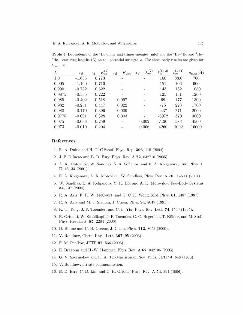
E. A. Kolganova, A. K. Motovilov, and W. Sandhas 145
Table 4. Dependence of the 4He dimer and trimer energies (mK) and the 4He–4He and 4He–4He2 scattering lengths (A) on the potential strength λ. The three-body results are given for
lmax = 0.
λ εd εd − E(1)ex εd − Evirt εd − E
(2)ex `
(1+2)sc `
(1+1)sc ρmax(A)
1.0 -1.685 0.773 - - 160 88.6 7000.995 -1.160 0.710 - - 151 106 9000.990 -0.732 0.622 - - 143 132 10500.9875 -0.555 0.222 - - 125 151 12000.985 -0.402 0.518 0.097 - 69 177 13000.982 -0.251 0.447 0.022 - -75 223 17000.980 -0.170 0.396 0.009 - -337 271 20000.9775 -0.091 0.328 0.003 - -6972 370 30000.975 -0.036 0.259 - 0.002 7120 583 45000.973 -0.010 0.204 - 0.006 4260 1092 10000
References
1. R. A. Duine and H. T. C Stoof, Phys. Rep. 396, 115 (2004).
2. J. P. D’Incao and B. D. Esry, Phys. Rev. A 72, 032710 (2005).
3. A. K. Motovilov, W. Sandhas, S. A. Sofianos, and E. A. Kolganova, Eur. Phys. J.D 13, 33 (2001).
4. E. A. Kolganova, A. K. Motovilov, W. Sandhas, Phys. Rev. A 70, 052711 (2004).
5. W. Sandhas, E. A. Kolganova, Y. K. Ho, and A. K. Motovilov, Few-Body Systems34, 137 (2004).
6. R. A. Aziz, F. R. W. McCourt, and C. C. K. Wong, Mol. Phys. 61, 1487 (1987).
7. R. A. Aziz and M. J. Slaman, J. Chem. Phys. 94, 8047 (1991).
8. K. T. Tang, J. P. Toennies, and C. L. Yiu, Phys. Rev. Lett. 74, 1546 (1995).
9. R. Grisenti, W. Schollkopf, J. P. Toennies, G. C. Hegerfeld, T. Kohler, and M. Stoll,Phys. Rev. Lett. 85, 2284 (2000).
10. D. Blume and C. H. Greene, J. Chem. Phys. 112, 8053 (2000).
11. V. Roudnev, Chem. Phys. Lett. 367, 95 (2003).
12. F. M. Pen’kov, JETP 97, 536 (2003).
13. E. Braatem and H.-W. Hammer, Phys. Rev. A 67, 042706 (2003).
14. G. V. Skorniakov and K. A. Ter-Martirosian, Sov. Phys. JETP 4, 648 (1956).
15. V. Roudnev, private communication.
16. B. D. Esry, C. D. Lin, and C. H. Greene, Phys. Rev. A 54, 394 (1996).

Few-Body Systems 0, 146–151 (2006) Few-Body
Systemsc© by Springer-Verlag 2006
Printed in Austria
Spectral observables for two and three-fold
symmetry breaking∗
M. S. Hussein∗∗,, J. X. de Carvalho, M. P. Pato and A. J. Sargeant
Instituto de Fısica, Universidade de Sao Paulo, Caixa Postal 66318, 05315-970, Sao Paulo, SP,Brazil
Abstract. We investigate the spectral statistics of a random matrix model forsymmetry breaking. It is pointed out that the spectral rigidity distinguishesmore clearly the breaking of two and three-fold symmetries than does thenearest neighbour spacing distribution.
1 Introduction
The experiments of Ellegaard and collaborators such as [1] have provided manyillustrations of the applicability of random matrix models to the spectral fluctu-ations in macroscopic acoustic resonators. In particular the effect of symmetrybreaking has been studied. The Rosenzweig-Porter model [2] describes transi-tions from the GOE to a superposition of independent GOEs. Here we studythis model for the transitions corresponding to two and three-fold symmetrybreaking and point out the relevance of these considerations to [1].
2 Model
The joint probability distribution of the matrix elements of a matrix, H, for andeformed Gaussian ensemble may be expressed as
P (H,A, B) = Z−1 (A,B) exp[−(A trH2 + B trH2
1
)], (1)
where Z is a normalisation factor and trH denotes the trace of H. The structureof the matrix H1 is chosen in such a way that it defines a subspace of H. The pa-rameters A and B define the energy scale and degree of deformation respectively.When B → 0 the joint distribution becomes
P (H,A, 0) = Z−1 (A, 0) exp(−A trH2
). (2)
∗Article based on the presentation by M. S. Hussein at the Fourth Workshop on the Dynamicsand Structure of Critically Stable Quantum Few-Body Systems, MPIPKS, Dresden, Germany,2005. Received December 6, 2005; Accepted December 16, 2005
∗∗E-mail address: [email protected]

M. S. Hussein, J. X. de Carvalho, M. P. Pato and A. J. Sargeant 147
When B → ∞, the elements of H1 vanish and H is projected onto a matrix,H0, whose elements are on the complementary subspace of H1. Therefore, therandom matrices generated by Eq. (1) are the sum of two terms
H = H0 + H1, (3)
and since tr(H0H1) = 0 the probability density may be written
P (H,A, B) = Z−1 (A,B) exp[−A trH2
0 + (A + B) tr H21
]. (4)
We are specifically interested in the case that H is real symmetric with H0
block diagonal and H1 coupling the blocks:
H0 =
H11
. . . 0Hbb
0 . . .Hmm
H1 =
0 H12 · · · H1m
H12. . . Hbb′
... 0
Hbb′. . .
H1m 0
(5)
The Hbb′ (b, b′ = 1, . . . m) are themselves Mb × Mb′ matrices. The probabilitydensity then becomes (we modify the variance of the bth block of H0 by a factorξb for later convenience)
P (H,A, B) = Z−1 (A,B) exp
−A
m∑b=1
ξ−1b
Mb∑ib=1
Hbb,ibib + 2Mb∑
ib<jb
Hbb,ibjb
+2 (A + B)
m∑b<b′
Mb∑ib=1
Mb′∑i′b=1
Hbb′,ibib′
(6)
and the normalisation constant for equal sized blocks is
Z(A,B) =
1
2Mb(Mb−1)
4
(π
ξ−1b A
)Mb(Mb+1)
4
m ( π
2(A + B)
)M2b
2
m(m−1)
2
.(7)
Consequently, the individual matrix elements have variance
H2bb,ibjb
=1 + δibjb
4Aξb, H2
bb′,ibib′=
14(A + B)
. (8)
This ensemble contains a transition from the GOE to a superposition of m GOEs.It is useful to introduce the parameter
α = (1 + B/A)−1/2 (9)
which measures the relative strength of H1 and H0. The transition from α=0 toα=1 corresponds to the transition from B=∞ to B=0.

148 Spectral observables for two and three-fold symmetry breaking
The average level density is found to be [3]
ρ (E) =m∑
b=1
gbρ1 (ab, E) , (10)
where ρ1 is given by
ρ1 (a,E) =
N
πa2/2
√a2 − E2, |E| ≤ a
0, |E| > a, (11)
a2b = a2
[ξbgb + α2(1− gb)
], (12)
N =∑m
b=1 Mb is the dimension of H, gb = Mb/N is the fractional density ofblock b and a =
√N/A is the radius of the Wigner semi-circle.
Choosing [4, 5]
ξb = 1 +N −Mb
1 + Mb(1− α2) −−−−→
N→∞1 +
1− gb
gb(1− α), (13)
it is found that ab = a, that is, the density is independent of α and is given byρ(E) = ρ1(a,E). The transition parameter utilised in the sections which followis defined as [6]
Λ = α2ρ(0)2 = α2 N2
πa/2. (14)
3 Nearest Neighbour Distribution
The nearest neighbour spacing distribution (NNSD) may be written [2]
p(s, 0) = pbb(s) + pbb′(s). (15)
Consider m blocks of equal dimension. Then
pbb(s) =1
m2p(s/m)E(s/m)m−1 (16)
and
pbb′(s) =(
1− 1m
)[1− Ψ(s/m)]2E(s/m)m−2. (17)
Leitner [5] obtained the perturbation formula
p(s, Λ) = pbb(s) + v(s, Λ)pbb′(s), (18)
where
v(s, Λ) = s
√π
8ΛI0(
s2
16Λ)e−s2/16Λ (19)
Note that sinceI0(x) ∼ ex
√2πx
, (20)

M. S. Hussein, J. X. de Carvalho, M. P. Pato and A. J. Sargeant 149
for large x, v(s, Λ) ∼ 1 for small Λ. For
p(s) =π
2se−πs2/4, (21)
ie. for individual blocks described by the Wigner surmise we have
1− Ψ(s) = e−πs2/4, E(s) = erfc(√
πs/2), (22)
so that
p(s, Λ) = se−π(s/m)2/4
[π
2m2erfc
(√πs
2m
)m−1
+(
1− 1m
)√π
8ΛI0(
s2
16Λ)e−s2/16Λe−π(s/m)2/4erfc
(√πs
2m
)m−2]
. (23)
It is in fact necessary to use the distribution
p(s, Λ, cN , cD) = cNp(cDs, Λ) (24)
where cN and cD are obtained by satisfying the conditions cN
∫∞0 p(cDs, Λ)ds = 1
and cN
∫∞0 sp(cDs, Λ)ds = 1 simultaneously for each Λ.
4 Spectral Rigidity
The spectral rigidity ∆s is a pure two-point observable which may be expressedin terms of the two-level cluster function Y2 by [7]
∆3(L,Λ) =L
15− 1
15L4
∫ L
0(L− r)3(2L2 − 9Lr − 3r2)Y2(r, Λ)dr. (25)
For the GOE, Y2(r) is given by [7]
Y2(r,∞) = s2 − (Si(πr)− πε(r))(c− s/πr), (26)
where s = sin(πr)/πr, c = cos(πr)/πr, Si(r) =∫ r0
sin ss ds and ε(r) =
1/20
−1/2.
Asymptotically, for the GOE we have [7]
∆3(L) = 1/π2(ln(2πL) + γ − 5/4− π2/8). (27)
For a superposition of m sequences of levels all with fractional densities 1/mthe spectral rigidity is given by [8]
∆3(L, 0) = m∆3(L
m,∞). (28)
Pandey [6] has obtained the formula
Y2(L,Λ) ≈ Y2(L,∞) + 2Λ
∫ ∞
−∞dL′
Y2(L′, 0)− Y2(L′,∞)(L− L′)2 + 4π2Λ2)
(29)

150 Spectral observables for two and three-fold symmetry breaking
which is valid for sufficiently large L and any crossover transition, the transitionbeing specified by the choice of the initial condition Y2(L, 0)[= 1
mY2( Lm ,∞) for
a m sequences of levels with fractional densities 1/m] and the final conditionY2(L,∞).
French et al. [9] had previous obtained results equivalent to Eq. (29) for sev-eral transitions. Leitner [5] used their result for the GOE to m GOEs transitionto obtain
∆3(L;Λ) ≈ ∆3(L;∞) +m− 1
π2
[(12− 2
ε2L2− 1
2ε4L4
)×ln(1 + ε2L2) +
4εL
tan−1(εL) +1
2ε2L2− 9
4
], (30)
ε =π
2(τ + π2Λ). (31)
For the cut off parameter we use the value [10] τ = cmeπ/8−γ−1, where cm =mm/(m−1) and γ ≈ 0.5772 is Euler’s constant. Both Eq. (25) in conjunction withEq. (29) and Eq. (30) agree well with numerical simulations for large L. The useof Eq. (25) together with Eq. (29) has the advantage that it is valid down toL = 0 (for finite Λ).
5 Results and Conclusions
In Fig. 1 we use the theoretical expressions from the previous two sections toplot the NNSD and the spectral rigidity for m = 2 and m = 3, correspondingtwo-fold and three-fold symmetry breaking, for several values of the symmetrybreaking parameter Λ. It can be seen that while the nearest neighbour spacingdistributions are qualitatively similar for m = 2 and m = 3, especially for thelarger values of Λ, the spectral rigidities for m = 2 and m = 3 are qualitativelydifferent for all the values of Λ considered. This suggests that the spectral rigiditydistinguishes more clearly the symmetry underlying a sequence of eigenvaluesthan does the NNSD.
In Ref. [11] a good fit of the NNSD of [1] to Eq. (24) with m = 2 was obtained.However inspection of the spectral rigidities of [1] reveals that they cannot befitted by Eq. (30) with m = 2. Abd El-Hady et al. [12] fitted both the NNSD andthe spectral rigidity of Ref. [1] using a model with three-fold symmetry which isdifferent from the one described here. While their model described the spectralrigidities well the fit they obtained of the NNSD was not as good.
The preceding discussion leads us to believe that the data of [1] should beanalysed using the Rosenzweig-Porter model as described here corresponding toa three-fold symmetry breaking. Such an analysis is under way.
Acknowledgement. This work was carried out with support from FAPESP and the CNPq.
References
1. C. Ellegaard et al., Phys. Rev. Lett. 77 (1996) 4918.
2. N. Rosenzweig and C.E. Porter, Phys. Rev. 120 (1960) 1698.

M. S. Hussein, J. X. de Carvalho, M. P. Pato and A. J. Sargeant 151
0 1 2 3 40
0.5
1P(s)
0 10 20 30 40 500
0.5
1
∆3(L)
0 1 2 3 40
0.5
1
0 10 20 30 40 500
0.5
1
0 1 2 3 40
0.5
1
0 10 20 30 40 500
0.5
1
0 1 2 3 40
0.5
1
s0 10 20 30 40 50
0
0.5
1
L
Figure 1. The left column shows the NNSD, calculated using Eq. (24) with Λ = 0.001 (top)
Λ = 0.01 (top-middle) Λ = 0.031 (bottom-middle) and Λ = 0.072 (bottom). The thin lines
are for m = 2 and the thick lines m = 3. The right column shows the corresponding spectral
rigidities calculated using Eqs. (30) and (27). The dotted lines on the bottom row are the
Wigner distribution Eq. (21) and Eq. (27).
3. A.C. Bertuola et al., Phys. Rev. E 71 (2005) 036117.
4. F.J. Dyson, J. Math. Phys. 3 (1962) 1191.
5. D.M. Leitner, Phys. Rev. E 48 (1993) 2536.
6. A. Pandey, Chaos, Solitons and Fractals 5 (1995) 1275.
7. M.L. Mehta, Random Matrices, 3rd ed. ed. (Academic Press, 2004).
8. C.E. Porter, Statistical Theory of Spectra: Fluctuations (Academic Press, 1965).
9. J.B. French et al., Ann. Phys. (N.Y.) 181 (1988) 198.
10. A.Y. Abul-Magd and M.H. Simbel, Phys. Rev. E 70 (2004) 046218.
11. D.M. Leitner, Phys. Rev. E 56 (1997) 4890.
12. A. Abd El-Hady, A.Y. Abul-Magd and M.H. Simbel, J. Phys. A 35 (2002) 2361.

Few-Body Systems 0, 152–156 (2006) Few-Body
Systemsc© by Springer-Verlag 2006
Printed in Austria
Critical stability effects in epidemiology∗
H. Hogreve∗∗
IFISR, International Foundation for Independent Scientific Research, 1133 Broadway, Suite706, New York, NY 10010, U.S.A.
Abstract. Basic properties of the epidemic and endemic version of the SIRmodel are described and the stability behaviour of the deterministic equilibriaunder random perturbations is studied. Domain restrictions of the dynamicalvariables lead to stochastic differential equations with boundary conditions,for which some characteristic numerical results are presented.
The mathematical description of the spreading of infectious diseases usuallyleads to epidemic models exhibiting phenomena akin to critical stability in phys-ical systems. Rather than pertaining to bonding between particles, in epidemiol-ogy critical stability arises from interactions between infective pathogenic agentsand susceptible hosts within a population. In one of the basic epidemiologicalmodels, viz., the SIR model [1, 2, 3], the considered population is classified intothree ”compartments” containing, respectively, S susceptibles, I infectives (i.e.,infected and infectious), and R removed individuals (i.e., individuals that havebeen killed by the disease or have acquired permanent immunity after recovery).Focusing onto a closed population, N = S(t) + I(t) + R(t) = const for all timest ≥ 0, and assuming a pseudo mass-action for the transmission of the disease,the two independent SIR equations for the fractions st = S(t)/N, it = I(t)/Nbecome
st
dt= −βstit + µ− µst,
itdt
= βstit − γit − µit. (1)
Here, β > 0 denotes the contact rate, γ > 0 the removal rate, and by thebirth/death rate µ ≥ 0 a possible demographic turnover through natural birthsand deaths is implemented. The following theorem collects crucial results [1, 3]
Theorem 0.1. For initial conditions s0, i0 ∈ TSI = (s, i) | s, i ≥ 0, s + i ≤ 1unique solutions (st, it) exist and belong to the triangle TSI for all t ≥ 0. SettingR0 = β/(γ + µ) and assuming µ > 0, then, if R0 ≤ 1 or i0 = 0, the (st, it)converge to the disease-free equilibrium (sdf , idf) = (1, 0) as t → ∞, whereas, if
∗Article based on the presentation by H. Hogreve at the Fourth Workshop on the Dynamicsand Structure of Critically Stable Quantum Few-Body Systems, MPIPKS, Dresden, Germany,2005. Received November 12, 2005; Accepted December 9, 2005
∗∗E-mail address: [email protected] and [email protected]

H. Hogreve 153
R0 > 1 and i0 > 0, the solutions approach the endemic equilibrium (sen, ien) =(1/R0, µ(R0 − 1)/β) as t → ∞. In case of µ = 0, st decreases monotonicallytoward s∞ = limt→∞ st (determined as unique root within (0, 1/R0) of s0 + i0 −s∞ + R−1
0 log(s∞/s0) = 0). Moreover, if R0s0 ≤ 1, then limt→∞ it = 0, or, ifR0s0 > 1, then it first increases to a maximum s0 + i0− (1 + log(R0s0))/R0 andthen decreases to zero as t →∞.
The quantity R0 is called the ”basic reproduction ratio” and plays a centralrole in epidemiological studies. Usually being defined as the average number ofsecondary infections produced by one infectious individual (during its averageperiod of infectiousness) in a completely susceptible population, here it emergesas one of the eigenvalues of the linearization of the dynamical system (1) at thedisease-free equilibrium. According to the theorem above, epidemic outbreaks canonly occur above the threshold R0 = 1. While for µ = 0 there is a single outbreak,the regime µ > 0 models an endemic with multiple (minor) outbreaks followingthe first major one. Further details and also applications of the SIR model toconcrete situations (e.g., measles) are discussed amply in the literature [1, 2, 3].
On the other hand, apparently there is not much known about the stabilityof the model under – in reality inevitable – random perturbations (see, e.g.,[4] and references therein for a motivational discussion). Stochastic effects canarise from the environment, i.e., sources external to the disease population, beingimplemented as random perturbations of the model parameters β, γ, or µ. Thesecond way of stochasticity to enter the model is via random perturbations ofthe basic variables themselves. Then the states of the epidemic become randomvariables whose evolution obeys stochastic differential equations. To account forrandom perturbations of the infectives, the second equation of the system (1)may be modified into
dit = (βstit − γit − µit)dt + a dWt (2)
where Wt stands for a standard Wiener process and a ≥ 0 for the intensity ofthe noise. Stability properties of the equilibria of equation (1) can be investi-gated with the help of the generalisation of the Lyapunov function to stochasticcalculus. Thus, to demonstrate that for a given stochastic differential equa-tion dXt = F (t, Xt)dt + B(t, Xt)dWt an equilibrium Xe of its deterministicpart dXt = F (t, Xt)dt remains stable in probability, it suffices to find a func-tion V ∈ C2(Rn,R+), positive definite on a neighbourhood of Xe and withV (Xe) = 0, such that the (stochastic) derivative LV along the trajectories obeysLV := ∇V ·F + 1
2TrBT (∇∇V )B ≥ 0 (where Bt denotes the transpose of B and∇∇V the Hessian of V ) [5]. In fact, choosing V (s, i) = s+ i− sdf − sdf log(s/sdf)shows that for all α ≥ 0 the disease-free equilibrium (sdf , idf) of equation (1)remains stable under the perturbations embodied in equation (2). However, ob-serving that – in particular for small it – the time evolution governed by equa-tion (2) does not respect the nonnegativity of it, this stability result is of onlylimited applicability. To retain the correct interpretation of it as fraction of apopulation, we have to impose a cutoff at zero and replace (2) by
it = max0, i0 +∫ t
0
(βsτ iτ − γiτ − µiτ
)dτ + a
∫ t
0dWτ. (3)

154 Critical stability effects in epidemiology
50 100t
0.2
0.4
0.6
0.8
1
s
0.2 0.4 0.6 0.8a
0.3
0.6
0.9
sasy
Figure 1. In the left part, two sample paths of st are plotted for µ = 0 with a = 0.1 (upper
curve) and 0.5 (lower curve). The right part contains curves sasy =< limt→∞ st > for µ =
0.01, 0.05, 0.1 and 0.2 (from top to bottom) as a function of the noise intensity a. In all cases the
stochastic differential equation was solved for β = γ = 1 and initial conditions (s0, i0) = (1, 0).
0.34 0.35 0.36 0.37s
0.022
0.024
0.026
0.028
0.032
0.034
i
0.3 0.4 0.5s
0.01
0.02
0.03
0.04
0.05
0.06
i
Figure 2. For β = 3 = 3γ and µ = 0.05, in the (s, i) phase plane a deterministic orbit (a = 0)
spirals toward the endemic equilibrium (left part), whereas a noisy limit cycle emerges for
a = 0.1 (right part).
This amounts to constructing a process that solves equation (2) (together withthe first part of equation (1)) and obeys a reflection-like (with possible timedelay) boundary condition at i = 0 [6] (see [7] for a discussion of the hittingtime of the boundary). Unfortunately, the established mathematical techniquesfor studying stochastic stability are not directly applicable for such processes.Nonetheless, these equations are accessible to standard numerical methods [8].
Considering µ = 0 with β = γ = 1 and thus R0 = 1, an epidemic is excludedfor the unperturbed system; numerical simulations for equation (3) show that alsothe random introduction of infectives does not lead to epidemic outbreaks. Sincenevertheless on the average the perturbations in equation (3) are tantamount ofa permanent inflow of infectives, all susceptibles eventually will be eradicated asFig. 1 indicates for a = 0.1 and 0.5. If µ > 0, in contrast to the situation forequation (2), upon adding random perturbations of the form (3) the disease-freeequilibrium loses its stability. However, due to the regeneration of susceptiblestheir number does not tend to zero for t → ∞. Rather, as displayed on theright hand side of Fig. 1, depending on the birth rate µ and noise intensity a,a balance between newborn and infected individuals develops and, on the longrun, produces a constant average < s∞ > of susceptibles.
In the unperturbed case, for µ > 0 and R0 > 1, there is an attracting equi-librium (sen, ien) to which all orbits (st, it) starting from i0 > 0 converge; anexample for β = 3γ = 3 is illustrated in the (s, i) phase plane plot in the leftpart of Fig. 2. Adding the stochastic perturbation, a > 0, this endemic equi-

H. Hogreve 155
librium is turned into a noisy limit cycle around (sen, ien). For a = 0.1, this isdepicted in the right part of Fig. 2; for larger a, due to larger amplitudes of theoscillations, both, the area explored by the orbits as well as their density in thisarea increase. The corresponding effects on the curve st are (irregular) oscilla-tions superimposed on the damped oscillations of the unperturbed a = 0 curve;for growing intensity a, these irregular oscillations become more violent andrapid, i.e., their amplitude and, by developing more and more spikes, also theirfrequency increase. Obviously there is a competition between the deterministicand stochastic dynamics; whereas the former always attracts the orbits towardthe deterministic equilibrium (sen, ien), by the latter the orbits get frequentlydisplaced into other directions.
Summarising, the scenario described here for the SIR model with randomperturbations looks similar to those encountered in other dynamical systemswith added stochasticity, like, e.g., the noisy Brusselator [9, 10]. The importantdifference, however, is caused by the boundary conditions expressed by equa-tion (3) that prevent employing results for standard Wiener processes and callfor appropriate extensions of the mathematical theory. With respect to concreteapplications, probably the results for the endemic model are of some practicalinterest; at (or below) the critical value R0 = 1, for realistic values of µ a detailedinvestigation can indicate how strongly a population would be affected (depend-ing on a) by ”nonvirulent” diseases. Likewise, taking R0 for a specific disease(e.g., R0 = 17 for measles), and including perturbations with small a values maylead to better insight when comparing model predictions with statistical datafrom empirical investigations.
Acknowledgement. Technical assistance by the Rechenzentrum der Universitat Hildesheim isgratefully acknowledged.
References
1. H.W. Hethcode, Three Basic Epidemiological Models, in: Applied MathematicalEcology, Eds. S.A. Levin, T.G. Hallam, L.J. Gross, Springer, Berlin, 1989.
2. R.M. Anderson and R.M. May, Infectious Diseases of Humans: Dynamics and Con-trol, Oxford University Press, Oxford, 1991.
3. H.W. Hethcode, Math. Biosci. 28 (1976) 335; SIAM Rev. 42 (2000) 599.
4. P. Rohani, M.J. Keeling, B.T. Grenfell, Am. Nat. 159 (2002) 469.
5. I.Ya. Kats, T.C.G. Fisher, Stability and Stabilization of Nonlinear Systems WithRandom Structures, Taylor and Francis, London, 2003.
6. I.I. Gikhman and A.V. Skorokhod, Stochastic Differential Equations, Springer,Berlin, 1972.
7. J. Grasman, O.A. van Herwaarden, Asymptotic Methods for the Fokker-PlanckEquation and the Exit Problem in Applications, Springer, 1999.
8. P.E. Kloeden, E. Platen, H. Schurz, Numerical Solution of SDE Through ComputerExperiments, Springer, Berlin, 2003.
9. Th.-M. Kruel, A. Freund, and F.W. Schneider, J. Chem. Phys. 93 (1990) 416.