arX

iv:q

uant

-ph/

0112

149v

1 2

3 D

ec 2

001

Emergence of particles from bosonic

quantum field theory

David Wallace∗

An examination is made of the way in which particles emerge fromlinear, bosonic, massive quantum field theories. Two different con-structions of the one-particle subspace of such theories are given,both illustrating the importance of the interplay between the quantum-mechanical linear structure and the classical one. Some commentsare made on the Newton-Wigner representation of one-particle states,and on the relationship between the approach of this paper and thoseof Segal, and of Haag and Ruelle.

Keywords: Quantum Field Theory; Particle Localization; Relativis-tic Quantum Mechanics

1 Introduction

For better or for worse, most quantum systems are found by starting witha classical system and then quantizing it. The states of the resulting quantumsystem will be described by complex functions on the configuration space of theclassical system, whose squared moduli tell us the probability density for findingthe system in a given configuration.

Applying this method to classical fields would seem, if not unproblematic,then at least difficult only for technical reasons. We would naturally expect tofind a theory whose states are wave-functionals on the configuration space: thatis, maps which associate a complex number to each configuration of the classicalfield on a given hypersurface.

Scarcely a vestige of this behaviour is seen in the usual phenomenology of‘quantum field theory’. Instead we find ourselves with a theory usually describedin terms of particles: quarks, gluons, electrons. . . , and the localized interactionsbetween them. The field-configuration viewpoint is occasionally seen (notablyin the path-integral formalism of quantum field theory) but is usually regardedas at best a calculational tool.

(December 23, 2001 )* Centre for Quantum Computation, The Clarendon Laboratory, University ofOxford, Parks Road, Oxford OX1 3PU, U.K.(e-mail: david.wallace@merton.ox.ac.uk).

1

Furthermore, these particles are notoriously strange entities. Various resultsof quantum field theory seem strongly to imply that they cannot be localizedin any meaningful, covariant way; that they must be created and annihilated ininteractions which cannot be spatio-temporally localized; that we cannot startwith a theory of free particles and ‘turn on’ an interaction without pathology(implying that the concept of particle is bound up with the dynamics of thetheory and is not just a kinematic concept); and that the particles which shouldbe associated with a given field theory vary according to the energy levels atwhich that theory is studied.

For these reasons, it is normal in modern quantum field theory to regardthe field as the primary concept and the particles as secondary, derivative enti-ties. This process has been studied extensively using the methods of algebraicquantum field theory and the signs are encouraging that it can be understoodin a mathematically and conceptually rigorous way; however, the very abstract-ness of these methods can make it difficult to understand quite why the idea of‘particle’ should be so powerful in understanding the prima facie very differentconcepts inherent in a quantised field.

The purpose of this paper, then, is to analyse in a fairly concrete contextthe way in which certain subspaces of a quantum field theory’s Hilbert spacecome to possess characteristics of a one-quantum-particle Hilbert space. ‘Theconcrete context’ in question is that of a massive, scalar, bosonic field, assumedto be asymptotically treatable as a free field. Section 2 presents the classicaland quantum theory of such a field, and section 3 considers what the correctdefinition should be of ‘local’ and ‘particle’ states in QFT. In sections 4–6 —which form the core of the paper — two separate constructions of the one-particle subspace are given, both of which illustrate the central role played bythe interaction between the linear structure on the QFT Hilbert space (presentin any quantum system) and the linear structure on the classical phase space(specific to a linear field theory). Section 7 discusses the Newton-Wigner rep-resentation of position for one-particle systems, and section 8 makes some briefcomments on the relationship between this paper’s approach to QFT and someother approaches; section 9 is the conclusion.

Currently, it is increasingly common for foundational discussions of QFTto be conducted in the powerful and abstract language of algebraic quantumfield theory. This paper eschews that tendency: some concepts and results ofalgebraic QFT are referred to, but the framework used here is much closer to thatused by the mainstream physics community. For a defence of the validity of usingthis apparently rather non-rigorous framework for a foundational discussion, seeWallace (2001b).

2 Field quantization

In this section, we shall review the method by which free, and weakly inter-acting, field theories are quantized. We shall outline the problems which occurwhen we try to reinterpret these quantized theories as fundamentally aboutparticles, and then consider, in qualitative terms, how particles can enter the

2

theory in a non-fundamental way.

2.1 Classical free fields

A fairly general second-order field equation for a free-field theory is

d2

dt2φ(x, t) +Rφ(x, t) = 0 (1)

where φ(x, t) is a real field defined on some manifold Σ × R, points on Σ arelabelled by x, and R is some real symmetric operator acting on functions of thespatial coordinate x.

The simplest example of such a theory is the real Klein-Gordon equation,for which

R = m2 −∇2, (2)

and in fact if we want a theory with relativistic covariance then there are no otherexamples. However, more general theories of this form are potential models for:

• Curved spacetimes with a time translation symmetry;

• Systems interacting with a time-independent background field;

• Solid-state systems.

Most crucially for our purposes, field theories with this form also occur as ap-proximations to nonlinear theories; we will consider this case in more detaillater.

Such a theory can be generated from a Lagrangian

L[φ, φ] =1

2

∫

Σ

d3x(φ(x)2 − φ(x)(Rφ)(x)

). (3)

Carrying out the Legendre transform to the Hamiltonian formalism, we geta set of canonical coordinates φ(x) labelled by x, a set of conjugate momentaπ(x), and a Hamiltonian H, where

π(x) =df

δL

δφ(x)= φ; (4)

H[φ, π] =1

2

∫

Σ

d3x(π(x)2 + φ(x)(Rφ)(x)

). (5)

Points in the phase space P of the field are then given by specifying pairs offunctions (φ, π); the Poisson bracket on P is given by

A[φ, π], B[φ, π] =∫

Σ

d3x

(δA

δφ(x)

δB

δπ(x)− δA

δπ(x)

δB

δφ(x)

), (6)

so of course φ and π obey the canonical relations φ(x), φ(y) = π(x), π(y) =0 and φ(x), π(y) = δ(x− y).

Through each point in phase space flows a unique trajectory; hence pointsin P are in one-to-one correspondence with solutions of (1).

3

2.2 Field quantization

We will quantize classical fields (free or interacting) in the most naive possi-ble way: by direct comparison with non-relativistic particle mechanics. That is,we will represent states of the quantum system by complex wave-functions onthe configuration space of the classical system. In this case, that configurationspace is the infinite-dimensional space S of functions on Σ, so the quantumstates will be functionals Ψ[χ] on this space (we will denote the Hilbert space ofall such functionals as HΣ). By analogy with the non-relativistic quantizationof the coordinates q, p as

qψ = qψ(q); pψ = −idψdq

(7)

we will quantize the coordinates φ(x) and π(x) as

(φ(x)Ψ)[χ] = χ(x)Ψ[χ]; (8)

(π(x)Ψ)[χ] = −i δΨ

δχ(x)[χ]. (9)

It is easy to check that the canonical commutation relations are satisfied:

[φ(x), φ(y)

]=[π(x), π(y)

]= 0; (10)

[φ(x), φ(y)

]= iδ(x− y). (11)

It is to be admitted that we have been very cavalier with our treatmentof the infinite-dimensional spaces in use here. It is possible (whilst we confineourselves to free fields) to be much more careful and rigorous,1 but if we wish ourframework to be powerful enough to handle interactions then there is actuallyno need for infinite-dimensional technicalities, for reasons to be explained insection 2.3.

2.3 Interactions and renormalisation

Formally speaking, nothing in the previous description will be altered if weadd some higher-order terms (such as φ4), which change the field equation fromfree to interacting: we could restrict our attention to regimes in which theseterms are small in comparison to the free-field Hamiltonian, and proceed toanalyse their effects using perturbation theory.

However, the reader may at this stage object that we are playing fast andloose with some very poorly-defined mathematical concepts. In fact, it is well-known that terms like φ4, when added to the Hamiltonian, give contributionswhich are not small, but infinite — hence formulating a well-defined interacting

1See Marsden and Ratiu (1994); Woodhouse (1991) for discussions of infinite-dimensionalclassical mechanics, and Wald (1994) for a careful discussion of quantising linear field theories.

4

quantum theory is actually very subtle. In fact, one approach would be to saythat the only quantum theories we understand well enough for conceptual studyare the free-field ones, and confine our attention to those.

In this paper, however, we shall take a more liberal attitude. There is actu-ally a well-defined approach to understanding these apparent infinities, workedout primarily by Kenneth Wilson and originating in solid-state physics. In Wil-son’s approach, we postulate that QFTs do not after all have infinitely manydegrees of freedom; rather, some unknown processes cut off the high-energydegrees of freedom and leave only finitely many to contribute to the physics.It then turns out — rather remarkably — that all interaction terms in theHamiltonian will fall into two categories. Non-renormalisable interactions willbe negligibly weak on energy scales far lower than the cutoff threshold. Renor-malisable interactions are not necessarily negligible, but at low energies theyare affected by the choice of the cutoff only through modifications (“renormali-sation”) of the parameters in the interaction terms. Since these parameters arein any case only known through experiment, the choice of the cutoff becomesirrelevant to the low-energy regimes of the QFT.

Solid-state physics provides an example of this process. If we study a solid-state system on length-scales which are large compared to the interatomic spac-ing, we can approximate the possible (classical) configurations of the atoms bya continuous function — and thus approximate the system by a continuous fieldtheory. In quantizing this theory we find that interaction terms lead to infinities,but these are an artefact of our continuum assumption. Once we introduce acutoff banning excitations of the system which vary significantly on length-scalesshort in comparison with the interatomic separation, the infinities vanish.

Because we are understanding field theories in this way, we can take a re-laxed attitude to the infinite-dimensional spaces which we will encounter in ouranalysis: such spaces are ‘really’ finite-dimensional, with the very short-distanceexcitations disallowed. As for the interaction terms, we will not have need oftheir specific forms. We shall just assume, where necessary, that such terms arepresent but that the theory has been renormalised and that, after renormali-sation, the interaction terms can be treated perturbatively. For details of themathematics of this process, see Peskin and Schroeder (1995) or any other QFTtextbook; for a conceptual discussion see Wallace (2001b).

2.4 Problems with a particle interpretation

The theory constructed above is undeniably a field theory, in the sensethat its configuration space, and fundamental observables, are inherently field-theoretic. It is, however, tempting to try to reinterpret the theory so as to makedirect contact with the particle concept, either by establishing some kind of‘duality’ between field and particle descriptions (in the same sense that there isa duality between position and momentum representations in ordinary quantummechanics, with neither representation being privileged over the other) or byreplacing the field description entirely with a particulate one (in which case,presumably, the field observables would just count as auxiliary constructions of

5

no direct physical significance).There are however, many problems which emerge as soon as we try to inter-

pret any QFT so as to incorporate particles at a fundamental level:

• The ‘elementary particles’ of particle physics are generally understood aspointlike objects, which would seem to imply the existence of positionoperators for such particles. However, if we add the requirement thatsuch operators are covariant (so that, for instance, a particle localised atthe origin in one Lorentz frame remains so localised in another), or the re-quirement that the wave-functions of the particles do not spread out fasterthan light, then it can be shown that no such position operators exist. (SeeHalvorson and Clifton (2001), and references therein, for details.)

• In non-relativistic quantum mechanics, it is straightforward to constructHamiltonians which describe particles interacting via long-range forces(for a simple example, consider two charged particles interacting via aCoulomb force). However, the concept of a long-range interaction primafacie requires some sort of preferred reference frame, which seems to castdoubt upon the possibility of constructing such an interaction in a rela-tivistically covariant way.

• As was mentioned in section 2.3, if interactions are present in a QFT thenit is necessary to work, not with the bare parameters in the Hamiltonian,but with ‘renormalised’ parameters — and the parameters which must berenormalised include some of those, such as charge, which are generallytaken to be intrinsic properties of particles. However, there is no priv-ileged way of renormalising the parameters, so that the values of theseparameters — and hence, the natures of the particles which they purportto describe — can be in part a purely conventional matter.

• When we consider quantum field theory on a general spacetime back-ground, there is no unique procedure to define particles, and states whichappear particulate in one reference frame do not do so in other refer-ence frames. For instance, consider the so-called ‘Unruh effect’, in whichthe Minkowski vacuum of a free QFT looks like a thermal (hence, non-particulate) state to a uniformly accelerating observer. In this exampleit may be possible to argue that non-inertial observers’ descriptions aresomehow less fundamental, but in a less symmetric spacetime there willbe no preferred class of observers available, hence no preferred definitionof particle. (For a more detailed account of this point, see Wald (1994),who advocates abandoning the particle concept as a consequence.)

Not all have abandoned particles as fundamental in view of these difficul-ties: Fleming has given a strong defence of the idea that particle localisationdoes indeed make sense in relativistic QFT (see Fleming (1996), Fleming andButterfield (1999), and references therein) and Weinberg’s recent QFT text-book (Weinberg 1995) explicitly begins with particles and constructs the fieldsas auxiliary objects. However, the general consensus in QFT (insofar as such

6

issues are ever explicitly addressed2) appears to be that the subject is primarilyabout quantum fields. In fact, much modern research in the field only reallymakes sense from this viewpoint: for example, consider lattice quantum chro-modynamics (which attempts to understand quark confinement and the exis-tence of protons and neutrons, but is formulated in terms of field configurationsand makes only limited contact with the elementary heuristic that a proton is‘just’ three particulate quarks bound together); or consider the quantum Sine-Gordon equation (Coleman 1985), which has two distinct particle descriptions(one fermionic, one bosonic) with the weak-field version of the one equivalentto the strong-field version of the other).

Of course, none of this is to deny that particles exist, merely that they arenot part of the fundamental ontology of quantum field theory. In the nextsection we will consider how it might be possible for the particle concept to berecovered from a field-theoretic description.

2.5 The particle as emergent concept

It is a central result of condensed-matter physics that, if we start with somemacroscopic collection of nonrelativistic particles close to some collective stablestate, small excitations from that state can often be treated in terms of creating‘particles’. It is also generally true that, for strongly interacting systems, these‘particles’ do not coincide with the particles from which the system is built: sovibrations in a crystal are described in terms of ‘phonons’, which are not crystalatoms, and quantized waves in a magnet are described in terms of ‘magnons’which are not iron atoms (Kittel and Fong 1987).

There are striking formal parallels with quantum field theory: in fact, theconstruction of phonons from a monatomic crystal is virtually the same as theconstruction of particle states in a massless, scalar quantum field theory. Thedifference is, the ontology of a crystal is not in question. It is definitely made upof the lattice atoms - which correspond to the field states at different space pointsin scalar QFT. Nonetheless many phenomena can be described by regarding thecrystal as a gas of phonons, and some — e. g. heat transport — require us tothink in terms of localized phonons (Kittel 1996).

There is nothing particularly paradoxical about this: the crystal isn’t ‘really’a gas of phonons, it’s just that certain states of the crystal have properties verysimilar to such a gas, and that treating these states as such is a great boon toanalysis of crystal dynamics. This puts phonons and their ilk in good company,for a great many objects in science — such as animals, or rigid bodies — haveto be understood in the same way. There are no perfectly rigid bodies, for in-stance (and they are certainly not part of the basic ontology of any fundamentalphysical theory), yet certain states of a many-particle system approximate thebehaviour of ‘ideal’ rigid bodies extremely well, and so deserve the name. (SeeWallace (2001a) for a more detailed discussion of this point.)

We shall adopt the same attitude to the particles of relativistic quantum

2See (Wilczek 1999) for an explicit statement of this consensus.

7

field theory: that is, we shall look for subspaces of the QFT Hilbert space inwhich the states have particulate properties. This will require us to formulatea definition of ‘particle’ and then to show that there are states of the QFTwhich approximately satisfy that definition; the rest of the paper is concernedwith this task. First, though, we need to consider in which situations we wouldexpect a QFT to appear particulate.

2.6 Particle regimes

The phenomenology of quantum field theory suggests two regimes in whichwe expect particle behaviour:

• The non-relativistic limit, in which the QFT appears to be describedby slow-moving particles interacting by long-range forces;

• The scattering limit, in which particles begin widely separated, interactby short-range forces, and at late times are again found in widely separatedstates.

We shall be concerned almost exclusively with the second case, for reasons ofmathematical tractability rather than on conceptual grounds: the analysis ofrelativistic fields via the methods of scattering theory is fairly well understood,whereas the process by which nonrelativistic quantum mechanics emerges asa limiting case of QFT is much more complicated. In the case of scatteringtheory, though, at times sufficiently long after (or before) the scattering event,the theory becomes very well approximated by a free quantum field theory.(This is intuitively plausible since for scattering theory to be applicable in thefirst place it is necessary that the nonlinear terms in the Hamiltonian constitute,after renormalisation, only a small perturbation to the free-field theory; for amuch more careful discussion and justification, see Haag 1996.)

For this reason, our analysis henceforth will be restricted to free quantumtheories (more specifically, to quantum theories of the form (1); this includessome sorts of background-field interactions).

3 Defining particles

In this section, we shall work out a definition of what properties a family ofQFT states ought to have in order to count as ‘particle’ states. Since the ideaof ‘particle’ is plainly at least connected to the concept of a localised state, webegin by considering how the latter states are to be defined in QFT.

3.1 Localised states in a field ontology

Which field-theory states are to count as localised?In a QFT the idea of localisation must enter through the spatial localisation

of the observables. The observables of the theory are defined via the field oper-ators φ(x, t) and π(x, t), so it is natural to define any given observable at time

8

t as being localised in a spatial region Σi ⊆ Σ iff it is a function only of fieldoperators of form φ(xi, t) and π(xi, t) with all of the xi in Σi.

But if defining localised observables is straightforward, defining localisedstates will prove decidedly less so. We might begin by trying:

Naive localisation: A state |ψ〉 is localised in a spatial region Σi

iff 〈φ| O |φ〉 = 0 for any observable O localised outside Σi.

This seems plausible when we compare it with the classical case: there a stateis localised in Σi if π(x) = φ(x) = 0 for any x /∈ Σi. But it is mathematicallyimpossible for any state to satisfy it, for it implies that for any such x, and forany n ∈ Z+,

〈ψ| φn(x, t) |ψ〉 = 〈ψ| πn(x, t) |ψ〉 = 0. (12)

But this would imply that |ψ〉 was a simultaneous eigenstate of π(x) and φ(x),and these operators have no eigenstates in common. (The mathematics, barsome need to regularise to deal with operators defined at a point, is the same asfor the nonrelativistic operators X, P , which are well-known to have no eigen-states in common.)

Physically it is easy to see what is happening here. The vacuum state of afield theory (which we will denote by |Ω〉) is not ‘nothingness’, or ‘empty space’;it is simply a slightly colourful way of describing the ground state of the field’sHamiltonian. In solid-state systems (which, recall, we are treating as field-theoretic systems like any other) this state is just the zero-temperature state ofthe solid, in which the atoms will not be at rest but will have zero-temperaturefluctuations; the same will be true for the field excitations of a relativistic fieldtheory.

This suggests, however, an alternative definition, first proposed (for space-time regions O, not spatial regions Σi) by Knight (1961):

Knight localisation: a state is localised in a spacetime region Oiff 〈φ| A |φ〉 − 〈Ω| A |Ω〉 = 0 for any observable A localised outsidethe light cone of O.

It is possible to find states satisfying this criterion (Knight 1961): take any

unitary operator U localised in O, then the state U |Ω〉 will be Knight-localisedin O.

However, Knight localisation differs in one important respect from the sortof localisation which we encounter in NRQM. In the latter, properties like ‘islocalised in O’ are treatable in the same way as properties like ‘has energy E’or ‘has momentum less than p’: that is, we can define a projection operatorwhose intended interpretation is ‘localised in O’, whose range is the space of allsuch states. This would be possible for Knight-localised states iff they form asubspace: that is, iff any superposition of two states Knight-localised in O isalso Knight-localised in O.

The fact that Knight-localised states do not have this property is a conse-quence of the Reeh-Schlieder theorem (Reeh and Schlieder 1961).

9

Reeh-Schlieder theorem: for any region O, the set of all statesgenerated by the action of operators localised within O upon thevacuum, spans the Hilbert space of the QFT.

(For a proof, and further discussion, see Haag 1996.) It follows3 from the Reeh-Schlieder theorem that states Knight-localised at O span the entire state space,which rules out any possibility of a projector meaning ‘localised with certaintyin O’.

It is easy to see — again by analogy to the solid state — why these problemsoccur. For in a generic solid-state system, atoms are coupled to their neighbours,and as a consequence the ground state of the system is highly entangled. Thisallows us (in principle) to exploit the long-range correlations between spatiallyseparated subsystems of the field to produce any state by local operations withinO.

(To see this process in a far simpler system, consider the four- dimensionalHilbert space HA ⊗ HB, where HA and HB are each one-qubit (two-state)systems. The entangled states

|φ±〉 = 1√2(|1〉⊗|1〉 ± |0〉⊗|0〉) (13)

are totally indistinguishable from one another when restricted to either sub-system (they both induce the reduced state ρ = 1

2 (|0〉 〈0| + |1〉 〈1|) on eachsubsystem) but their sum 1√

2(|φ+〉 + |φ−〉 = |1〉⊗|1〉 is clearly distinguishable

from both of them on either subsystem. Examples of this kind are analysed inrather more detail by Redhead (1995) and Clifton and Halvorson (2001).)

However, in practice the correlations due to vacuum entanglement usuallydrop off fast enough that using Knight-localised states to approximate stateslocalised far from O requires prohibitively high-energy states. We can then usethe following pragmatic criteria to characterise locality:

1. Effective localisation (qualitative form): A state |ψ〉 is

effectively localised in a spatial region Σi iff for any function f offield operators φ, π, 〈ψ| f |ψ〉 − 〈Ω| f |Ω〉 is negligibly small when fis evaluated for field operators outside Σi, compared to its valueswhen evaluated for field operators within Σi.

2. The effective localisation principle (ELP) (qualitativeform: A subspace H of the QFT Hilbert space HΣ obeys the ELPon scale L iff for any spatial region S large compared with L, asuperposition of states effectively localised in S is effectively localisedin effectively the same region.

3To see that it follows, we need only note that the unitary elements of a (bounded) operatoralgebra A(O) span A(O). This can be proved as follows: for any bounded Hermitian element

H of A(O), and any t 6= 0, (it)−1(exp(itH)− 1) is a linear combination of unitary elements of

A(O). As t → 0, this sequence tends to H, hence H is in the span of the unitary operators.

To complete the proof, simply recall that any linear operator can be written as A+ iB, where

A and B are Hermitian.

10

These qualitative notions can be made precise in a number of ways, such as:

1. Effective Localisation (quantitative form): A state is L-

localised in a region Σi, iff for any function f of field operatorsφ, π, 〈ψ| f |ψ〉 − 〈Ω| f |Ω〉 falls off for large d like (or faster than)exp(−d/L), where d is the distance from Σi at which the function

(f) is evaluated. (Note that there is no difference, according to thisdefinition, between a state L-localised at some spatial point x anda state L-localised in a region of size ∼ L around x.)

2. ELP (quantitative form): A state obeys the ELP on scaleL iff, for any 3-sphere S of radius > L, a superposition of statesL-localised in S is L-localised in S.

A subspace of states for which ELP holds on scale L can be treated —approximately — as possessing a well-defined concept of localisation and of“localised in Σi” projectors for regions large compared with L (these are con-structed, for each such region Σi, by taking the projector onto the set of allstates in H which are effectively localised in Σi; because of ELP, this set mustbe a linear space). Effectively, in such a subspace we are excluding enough statesthat for any sufficiently large Σi, we cannot construct states localised far fromΣi using only those states localised within Σi.

It is still reasonable to ask: what good is effective locality? A state effec-tively localised in A can still in principle be distinguished from the vacuumvia measurements made arbitrarily far away from A. This question lies ratheroutside the scope of this paper (see Halvorson and Clifton (2001) and Wallace(2001b) for further discussion). Here we note only that such problems are byno means new to relativistic quantum theory. Even in non-relativistic quantummechanics, there are in general no states which remain exactly localised in afinite region for any finite period of time — yet this does not seem to get in theway of the concept of localised particle in NRQM.

For the purpose of this paper, we shall treat effective localisation as ‘goodenough’, and (since no particularly useful concept of exact localisation exists)will often drop the word ‘effective’, treating effectively localised states simplyas localised.

3.2 What is a quantum particle?

Granted that a quantum field theory must be treated as being fundamentallyabout fields, what properties must a given state of a quantum field theory havein order to be deemed a particle state? It is instructive to start by consideringthe classical case: which classical field configurations (if any) could be describedas particles? Here the answer seems obvious: the ‘particle’ configurations willbe field configurations which are localised in a fairly small spatial region —localized blobs of field, in fact. Translated into quantum mechanics, this wouldmake ‘particles’ just another name for the effectively localised states of the lastsection, provided that they were localised to sufficiently small regions.

11

However, this classical concept of particle is in one sense too weak to beappropriate for quantum theory. Classical wave-packets tend to spread outwith time, becoming less localised — and hence, less ‘particulate’, whereas innon-relativistic quantum mechanics a state describing n particles at time t willcontinue to describe n particles at all other times — and even in relativisticquantum mechanics we wish to recover a notion of particle which is robust andtime-independent provided the particles are far away from one another.4

Furthermore, the criterion that particles should be localised is in some sensealso too strong for quantum mechanics. As the two-slit experiment reminds us,it is easy for a particle to enter a state which is nowhere near an eigenstate ofposition — in other words, nowhere near localised.

However, the two-slit experiment also suggests the correct quantum defini-tion of particle. Although the experiment shows — by demonstrating interfer-ence of the particle wave — that a classical-particle picture isn’t viable, it alsoshows that a classical-wave picture isn’t viable either, because on measurementthe particle is always found to be localised somewhere. To ensure within theformalism of quantum physics that this happens, it is enough to require theparticle to be a linear superposition of states all of which are localised — thenany measurement of particle position will always give a single answer. (I stressthat this is intended to be an essentially interpretation-independent statement:I am not addressing the measurement problem here.)

These observations motivate our definition of a quantum particle:5

A space of one-particle states of size L (where L is small), written H1P , is asubspace of the QFT Hilbert space HΣ such that

1. There is a basis for H1P , each member of which is a state L-localised ata point; equivalently, all states in H1P are linear superpositions of suchlocalised states.

2. H1P satisfies the effective localisation principle on scale L.

3. H1P is effectively preserved, on relevant timescales, by the dynamics ofthe field theory.

This definition is intentionally somewhat vague. The imprecision of the thirdcriterion mirrors the way in which quasi-particles arise in solid-state physics —often the quasi-particles spontaneously decay, so that the one-particle subspaceis not exactly preserved by the dynamics. However, provided that the decaytime is long compared to other relevant timescales (such as the time takenby the quasi-particles to move between collisions) then the quasi-particles will

4We can find classical field theories which contain states like these — the solitons of thesine-Gordon equation are one example (Coleman 1985) — but in general they occur onlyin strongly non-linear theories, whereas here we are concerned with linear or nearly lineartheories.

5It should be noted that this definition is closely related to the definition used in algebraicQFT, in which an n-particle state is defined as one which is able to trigger up to, but no morethan, n detectors at a time. See Haag (1996, section II.4 and chapter VI) for more on thisdefinition.

12

provide a useful concept with which to describe the field theory. As the decaytime decreases there will come a point at which this concept ceases to be useful,but it would be a mistake to try to define this point exactly.

We have also made no attempt to be precise about the phrase ‘where L issmall’: how small is small? In non-relativistic quantum mechanics, the answeris ‘arbitrarily small’: a (possibly overcomplete) basis can be constructed fromstates effectively localised in arbitrarily small regions of configuration space.(The set of all Gaussians of an arbitrary fixed width, for instance, will do nicely.)It will turn out, however, that this is not possible in quantum field theory: herethere will turn out to be a minimum realizable size. It is reasonable to think ofthis as giving the ‘size’ of a particle: a particle’s size is the size of the smallestregion in which it can be localised.

Is it justifiable to be this vague in our definitions? A robust answer wouldbe ‘it works for quasi-particles, so why not?’ More satisfactorily, we can recallthat we are not looking for particles which can be added to the basic ontologyof our theory (which, granted, does need precise definition); the basic ontologyis and remains states of HΣ, or equivalently, wave-functionals on S. Rather,we are just finding a good way to characterise certain states with interestingproperties. Provided these states are picked out very accurately, there is noneed to worry if the accuracy isn’t perfect: we are simply looking for accurate,robust schemes by which we can approximate the dynamics of the theory andexplain phenomena. (For a more extended, and somewhat more philosophical,defence of this use of approximate concepts in physics, see Wallace 2001a.)

In any case, it is the existence of an H1P simultaneously satisfying (1), (2)and (3) which is in need of explanation. A space satisfying any given one ofthese clauses would not be particularly remarkable: for instance, given anycollection of localised states we could construct a space satisfying (1) by takingtheir span, but then this space would not generally be preserved under time-evolution; or we could construct a space satisfying (3) by taking the collectionof all states which are time-evolutes of our given collection, but then generallynot all such states would be linear superpositions of members of the originalcollection. Furthermore, if our system satisfied (1) and (3) but not (2), we wouldhave no guarantee that the concept of localisation would work for our particlesas we need it to do in non-relativistic quantum mechanics and in scatteringtheory: specifically, we would have no guarantee of the existence of projectionsonto particles in a specific location.

In the next three sections, we will go about constructing states which fit thedefinition of a particle given above. Before embarking on this task, though, weshould address an obvious objection: that we know perfectly well which statesof a free QFT are the one-particle states, so all that is left to do is verify thatthe definition holds for these states.

The results of the ensuing calculation would, of course, confirm that freeQFTs have one-particle sectors; however, it would not really answer the questionof why they do. The more indirect approach used here is intended to give someinsight into this second question.

13

4 Modal analysis of a free field

This section is a mathematical analysis of the structure of classical linearfield theories; it is a common ‘building block’ for the two methods of reachingthe one-particle subspace which will be developed in sections 5 and 6.

For the sake of mathematical rigour, this section makes some use of distri-bution theory (all such material can safely be skipped by any reader who doesnot get nervous upon sighting a Dirac delta function). The notation and ter-minology used is essentially that of Rudin (1991), especially chapters 6–7; inparticular, use is made of Rudin’s elegant ‘multi-index’ notation, in which

• an index α stands for an ordered n-tuple (α1, . . . , αn) with αi ∈ Z+;

• Dα :=(

∂∂x1

)α1 · · ·(

∂∂xn

)αn;

• |α| := α1 + · · ·+ αn.

4.1 Required properties of R

Recall that the free-field theories we are considering have the field equation(1), i. e.

d2

dt2φ(x, t) +Rφ(x, t) = 0.

We begin our analysis with a technical digression onto the operator R in thisfield equation. Specifically we will require the operator to have the followingproperties:

1. R is a continuous linear map from C∞(Σ), the space of real smooth func-tions on Σ, to itself.6

2. R can be extended to a self-adjoint operator on (a dense subspace of)the space L2(Σ) of square-integrable complex functions on Σ. (We shallidentify R with its self-adjoint extension).

3. R is a local operator, in the sense that Rf(x) depends only on the valuesof f in an arbitrarily small neighbourhood of x.7

4. The spectrum of R is known to be real, since it is self-adjoint; we shall alsorequire it to be positive and to be bounded below by a strictly positiveeigenvalue. (In other words, zero is not an eigenvalue of R; hence, R isinvertible).

6‘Continuous’ means ‘continuous with respect to the topology on C∞(Σ) induced by thefamily of semi-norms pN (f) = sup|Dαf(x)| : x ∈ Σ, |α| ≤ N’; see Rudin (1991, pp. 34–36)for more on such topologies.

7Given the short-distance cutoff introduced in section 2.3 to make mathematical sense ofinteracting QFTs, the requirement of exact locality is not really necessary: it is enough torequire that Rf(x) depends significantly on the values of f only in a neighbourhood of width∼ Lcut, where Lcut is the cutoff lengthscale; anticipating the later results of this section, thisis to require that R is Lcut-local.

14

If the spectrum of R is discrete, R must have a complete set of eigenfunc-tions, orthonormal in the L2 inner-product

〈φ, ψ〉 ≡∫

Σ

d3xφ∗(x)ψ(x); (14)

we will denote a given such set as fk(x). (Note that since R is both real andself-adjoint we can always choose its eigenfunctions to be all real, though weshall not always do so.) The eigenvalue of fk is denoted ω2

k, with ωk > 0.We will, in fact, take a somewhat schizophrenic attitude towards the dis-

creteness (or otherwise) of the spectrum of R: for conceptual analysis it willusually be convenient to take it as discrete, but in practical applications wewill often want to take R to be a differential operator on R3, in which case thespectrum is necessarily continuous. We shall therefore take the usual (if some-what non-rigorous) physicist’s step of assuming that moving from a discrete toa continuous spectrum is a purely technical matter involving no change in theconceptual situation.

Now, let x be any point on Σ; then we can define a linear functional Rx onC∞(Σ) by Rx · f = (Rf)(x); the continuity of R means that Rx is continuous,hence is a distribution (generalised function) over C∞(Σ). The following resultsare easy consequences of distribution theory and of the locality of R:

1. Because R is local, each Rx has support x.

2. From theorem 6.25 of (Rudin 1991) we can deduce that (in a local chartat x), we can find constants cα and N such that Rx =

∑|α|≤N cαD

αδx,where δx is a Dirac delta at x.

3. From the continuity of R, it follows that, in any local chart, we can findfunctions cα(x) such that, for any x in the chart,Rx =

∑|α|≤N cα(x)D

αδx.

4. From this, we deduce the (fairly obvious) fact that R is a differentialoperator.

If we follow the usual fiction of treating distributions as functions, we can(formally) define a function R(x,y) by

∫

Sd3yR(x,y)f(y) ≡ Rx · f ; (15)

hence

(Rf)(x) =∫

Sd3yR(x,y)f(y). (16)

Again formally, we can think of this function as giving the matrix elements ofR in a position basis, provided we remember that these elements are derivativesof delta functions.

It follows from the spectral theorem that

R(x,y) =∑

k

ω2kfk(x)f

∗k (y), (17)

15

and that the kernels Rλ(x,y) of the operators Rλ are given by

Rλ(x,y) =∑

k

ω2λk fk(x)f

∗k (y). (18)

(Again, these kernels may well be delta-functions or other such distributions;they are not necessarily well-behaved functions.)

Fractional powers of R will become important later in the paper, and in gen-eral such operators will not be exactly local even ifR is (the operator

√m2 −∇2,

for instance, is known (Goodman and Segal 1965) to be anti-local, in the sensethat for any function f , supp

√m2 −∇2f ∪ suppf is all of space except possibly

for a set of points of measure zero) but they may be ‘approximately local’. Wedefine ‘approximately local’ as follows:

An operatorR is L-local iff its kernelR(x,y) drops off like exp(−|x− y|/L)as |x− y| becomes large compared with L .

Informally, this means that while Rf(x) does not just depend on the values off in an arbitrarily small neighbourhood of x, it does depend significantly onthe values of f only in a neighbourhood of width ∼ L. Note that there is acertain looseness in the definition (in the phrase ‘large compared with’); purelymathematically, we could replace this with ‘as |x−y| → ∞’ but clearly it wouldbe against the spirit of the definition for (say) the kernel to start dropping offonly once |x− y| ≫ 1030L.

In the next section we will prove approximate locality for an importantsubclass of R operators.

4.2 Euclidean-invariant R

In this section we will consider an important sub-class of R operators: thosewhich act upon R3 and which are invariant under spatial translations and ro-tations. In this context we can establish the approximate locality of the Rλ

operators.The reason for requiring translation invariance is that we can work in Fourier

space: any translation-invariant operator must have the exponential functions1

(2π)3/2exp(ik · x) as its eigenfunctions and so from (17) we must have

R(x,y) = 1

(2π)3

∫d3k exp(ik · (x− y))ω2(k). (19)

Since R(x,y) is a rotationally-invariant sum of derivatives of delta functions,it follows that the function ω2(k) is a polynomial in k · k. Formally, then, theintegral (19) can be transformed to

R(r) = 1

(2π)2ir

∫

R

dk k ω2λ exp(ikr) (20)

where r = |x − y| and where we have replaced R(x,y) with R(r) to indicatethat R depends on x and y only through r. For positive λ at least, this integral

16

is divergent, indicating that R(r) is distributional; however, if the spectrum isunbounded then for sufficiently negative λ then the integral becomes convergent.

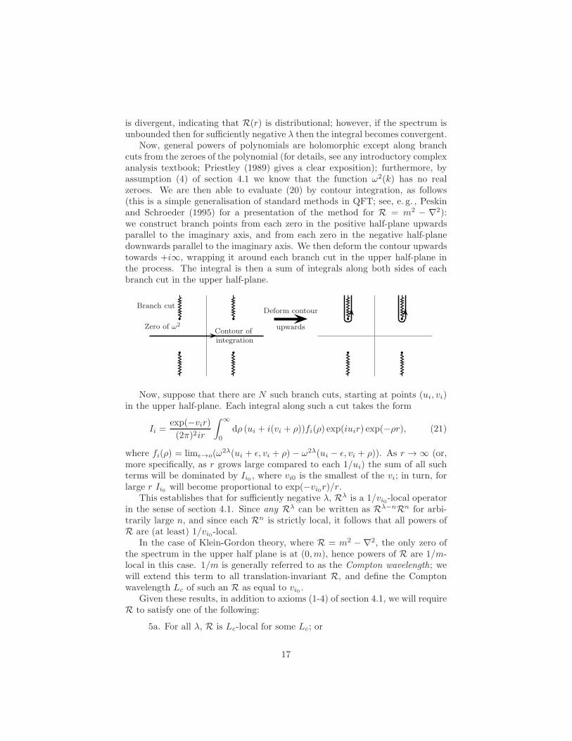
Now, general powers of polynomials are holomorphic except along branchcuts from the zeroes of the polynomial (for details, see any introductory complexanalysis textbook; Priestley (1989) gives a clear exposition); furthermore, byassumption (4) of section 4.1 we know that the function ω2(k) has no realzeroes. We are then able to evaluate (20) by contour integration, as follows(this is a simple generalisation of standard methods in QFT; see, e. g. , Peskinand Schroeder (1995) for a presentation of the method for R = m2 − ∇2):we construct branch points from each zero in the positive half-plane upwardsparallel to the imaginary axis, and from each zero in the negative half-planedownwards parallel to the imaginary axis. We then deform the contour upwardstowards +i∞, wrapping it around each branch cut in the upper half-plane inthe process. The integral is then a sum of integrals along both sides of eachbranch cut in the upper half-plane.

Branch cut

Zero of ω2

Contour ofintegration

Deform contour

upwards

Now, suppose that there are N such branch cuts, starting at points (ui, vi)in the upper half-plane. Each integral along such a cut takes the form

Ii =exp(−vir)(2π)2ir

∫ ∞

0

dρ (ui + i(vi + ρ))fi(ρ) exp(iuir) exp(−ρr), (21)

where fi(ρ) = limǫ→o(ω2λ(ui + ǫ, vi + ρ) − ω2λ(ui − ǫ, vi + ρ)). As r → ∞ (or,

more specifically, as r grows large compared to each 1/ui) the sum of all suchterms will be dominated by Ii0 , where vi0 is the smallest of the vi; in turn, forlarge r Ii0 will become proportional to exp(−vi0r)/r.

This establishes that for sufficiently negative λ, Rλ is a 1/vi0-local operatorin the sense of section 4.1. Since any Rλ can be written as Rλ−nRn for arbi-trarily large n, and since each Rn is strictly local, it follows that all powers ofR are (at least) 1/vi0-local.

In the case of Klein-Gordon theory, where R = m2 − ∇2, the only zero ofthe spectrum in the upper half plane is at (0,m), hence powers of R are 1/m-local in this case. 1/m is generally referred to as the Compton wavelength; wewill extend this term to all translation-invariant R, and define the Comptonwavelength Lc of such an R as equal to vi0 .

Given these results, in addition to axioms (1-4) of section 4.1, we will requireR to satisfy one of the following:

5a. For all λ, R is Lc-local for some Lc; or

17

5b. R is rotationally and translationally invariant.

Of course, 5b implies 5a.It might appear that solid-state systems do not satisfy 5b since the lattice

structure violates translational and rotational invariance, but in fact the latticeonly enters the observable results of the theory by imposing a short-distancecutoff, and hence (provided we work at lengthscales large compared with thecutoff) most solid-state systems may be treated as satisfying 5b.

4.3 Modes of the free field

Recall how to solve the free-field equation (1) by separation of variables: wetry an ansatz of form ψ(x, t) = A(x)B(t); this gives

A(x)B(t) +B(t)RA(x) = 0. (22)

Dividing through by A(x)B(t) splits the equation into two terms, one indepen-dent of x and the other of t; this means that the equation can be solved onlyby finding solutions to the paired equations

B + ω2B = 0; (23)

RA = ω2A (24)

where ω is to be determined. The second of these is simply the eigenfunctionequation for R. Each mode will have either exponential decay/growth (forω2 < 0), or sinusoidal variation (for ω2 > 0), in time; our restriction to positiveR eliminates the former case (this is the reason for this restriction) and we areleft with a set of solutions of the form

φ(x, t) = fk(x) cos(ωkt) (25)

andφ(x, t) = fk(x) sin(ωkt). (26)

(For the Klein-Gordon equation, the fk are just proportional to sine and cosinefunctions sin(k · x), cos(k · x), with the possible values of k constrained by theboundary conditions and with ω2

k = m2 + k · k.)An arbitrary solution of the equations can be expressed as a sum of solutions

of this form:

φ(x, t) =∑

k

1√ωk

(qkfk(x) cos(ωkt) + pkfk(x) sin(ωkt)) , (27)

so that a solution is given by the collection of real numbers (qk, pk).Since the space of solutions to the field equations is in one-to-one correspon-

dence with the phase-space P (via φ(x) ≡ φ(x, 0), π(x) ≡ φ(x, 0)) we can regard(qk, pk) as coordinatizing P : to be specific, we have

φ(x) =∑

k

1√ωkqkfk(x) (28)

18

andπ(x) =

∑

k

√ωkpkfk(x). (29)

In fact, the choice of√ωk factors in (27) means that they are canonical

coordinates, in the sense that they obey the Poisson-bracket relations qk, qk′ =pk, pk′ = 0; qk, pk′ = δk,k′ (the proofs are straightforward and make use ofthe orthonormality of the fk). In these coordinates the Hamiltonian (5) becomes

H =1

2

∑

k

ωk(p2k + q2k). (30)

Thus, subject to our restrictions on R at the start of section 4.1, any free-fieldtheory can (as is of course well-known) be expressed as a sum of independentharmonic oscillators.

If we define αk = 1√2(qk + ipk) we can rewrite (27) in the alternative form

φ(x, t) =∑

k

1√2ωk

(αkfk(x) exp(iωkt) + α∗kf

∗k (x) exp(−iωkt)) . (31)

In fact, there is no real reason to restrict to real-valued eigenfunctions fk: theexpansion (31) is just as valid for complex eigenfunctions. Inverting it gives

αk =1√2

∫

Sd3x f∗

k (x)

(√ωkφ(x) − i

1√ωkπ(x)

), (32)

which (following the definition αk = 1√2(qk + ipk) in the real-fk case) suggests

taking

qk =

∫

Sd3x

(√ωkφ(x)Refk(x) +

1√ωkπ(x)Imfk(x)

)(33)

and

pk =

∫

Sd3x

(−√ωkφ(x)Imfk(x) +

1√ωkπ(x)Refk(x)

)(34)

in the complex case. We can readily show that these are still canonical coor-dinates; the forms of (27–29) become slightly more complicated but H still hasthe form (30). This generalisation is useful in the Klein-Gordon equation, forinstance, as it allows us to take fk ∝ exp(ik·x), which is usually mathematicallymore convenient than working with sine and cosine functions.

The coordinate functions qk and pk have very simple time-dependence: fromthe Poisson brackets, we have qk = ωkpk and pk = −ωkqk. Hence the time-evolution of the system is

qk(t) = qk(0) cos(ωkt) + pk(0) sin(ωkt); (35)

pk(t) = pk(0) cos(ωkt)− qk(0) sin(ωkt), (36)

or equivalentlyαk(t) = αk(0) exp(−iωkt). (37)

19

5 Particles through coherent states

The first method which we will use to construct particle states begins byconstructing quantum-mechanical approximations to classically localised fieldstates. In fact, it will turn out that these approximations are not particles, butthey provide a natural stepping stone towards particles.

5.1 Harmonic oscillator coherent states

For a linear field theory, note that even in the classical case there are stateswhich are localized to greater or lesser degrees. For instance, plane waves are(improper) classical states which are not localized at all, whereas we can con-struct fairly localized wave-packets. This is different from the case of particlequantum mechanics, where the classical states are perfectly localized and anyloss of localization occurs only at the quantum level.

One way to construct a localized quantum state might be as follows: we beginby choosing a point in the classical phase space which is fairly localized (e. g. afairly compact classical wave-packet) and then try to construct a quantum statewhich is concentrated around this point. Obviously, in the general case there isno unique way of approximating a phase-space point in quantum mechanics sinceprecise localization in phase-space is not a well-defined quantum concept. In thecase of a harmonic oscillator, however, there is a simple prescription(Glauber(1963); see Peres (1993) for a discussion) which generates approximations to

phase-space points. If a† is the creation operator for such an oscillator and |0〉is its ground state, then the state

|α〉 = exp(−|α|2/2) exp(αa†) |0〉 (38)

has the following properties:

1. It is a Gaussian in both position and momentum space;

2. It is centred around q =√2Reα in position space, and p =

√2 Imα in

momentum space;

3. In both position and momentum space, the wave packet keeps its shapeunder time evolution (i. e. remains a Gaussian of the same width);

4. As time passes, the centres of the Gaussian in position and momentumspace evolve as would the position and momentum of a classical harmonicoscillator with the same Hamiltonian.

Such a state is called a coherent state. Note that because of the one-to-onecorrespondence between phase space and the set of solutions to the dynamicalequations, and because the coherent states track the classical evolution of phasepoints, we may equally well regard coherent states as quantum approximationsto classical solutions.

20

5.2 Field coherent states

Since the free field is (mathematically speaking) a collection of independentharmonic oscillators, these coherent states are an appropriate tool to constructquasi-classical states. The kth mode has creation operator a†k(=

1√2(qk − ipk)),

and hence a basis for the field Hilbert space HΣ is given by the states createdby successive actions of the different a†k on the vacuum.

A state localized around the kth mode would be

Dk(α) |Ω〉 := exp(−|α|2/2) exp(αa†k) |Ω〉 (39)

where the classical mode being approximated is (Reαfk/√ωk, Imαfk

√ωk).

Similarly, a classical state made from a superposition of modes may be quantum-mechanically approximated by successive application of Dk operators to thevacuum, and the evolution of the classical state will be tracked by the quantumwave-packet.

It is vital to keep in mind the differences between classical and quantumconcepts in what we are doing. Remember, we are constructing a quantumwave-packet, a complex functional on the space of field configurations, whichis concentrated around a given point in configuration space. That point itselfdescribes a classical wave-packet, that is, a real function on physical, three-dimensional space.

As time passes, the quantum wave-packet will not spread out across con-figuration space but will move around keeping its shape. Its centre will movethrough the configuration space according to the classical equations of motion,which will entail the spreading out through physical space of the classical wave-packet. Thus a coherent state will become less localized in physical space withtime even though the quantum wave-functional keeps its shape (and, in partic-ular, its width) in configuration space.

Now suppose the classical solution which we want to approximate is

φ(x, t) =∑

k

1√2ωk

(αkfk(x) exp(iωkt) + α∗kf

∗k (x) exp(−iωkt)) , (40)

and that it corresponds to the phase-space point (φ, π); then the correspondingcoherent state is

|C(φ, π)〉 =∏

k

Dk(αk) |Ω〉 (41)

(the order in which the Dk(αk) are applied is irrelevant as they all commute).Writing this out explicitly, we get

|C(φ, π)〉 =∏

k

(exp(−|αk|2/2) exp(−αka

†k))|Ω〉 (42)

which may equally well be written as

|C(φ, π)〉 = exp

(−1

2

∑

k

|αk|2)exp

(−∑

k

αka†k

)|Ω〉 . (43)

21

All we have used here is the elementary fact — applicable also to commutingoperators — that a product of exponentials is equal to the exponential of thesum of their arguments.

Now if we take (φ, π) to be an element of P satisfying∑

k |αk|2 = 1, we candefine

a†(φ,π) =∑

k

αka†k (44)

andD(φ,π)(z) = exp(−|z|2/2) exp(za†(φ,π)). (45)

then we will have|C(φ, π)〉 = D(φ,π)(1) |Ω〉 . (46)

Acting on the vacuum with D(φ,π)(z) for higher values of |z| creates coherentstates localized around successively larger wave-packets; in this way, the actionof D(φ,π)(z) on the vacuum as we vary |z| and hold (φ, π) fixed will map outa collection of states, whose span is a subspace of HΣ. It is easy to see thatthis space can also be spanned by those states generated from the vacuum bysuccessive action of the a†(φ,π) operator. Structurally there is a strong similarity

to the subspaces created by the a†k, although of course this new subspace is notpreserved by time evolution.

5.3 Coherent states are not particles

Can the coherent states be regarded as quantum particles? Absolutely not.Although there are more and less localised non-relativistic quantum particles,and more and less localised coherent states, the two forms of localisation arewildly different. If (φ, π) and (φ′, π′) are phase-space points localised in differentregions8 of Σ then (φ + φ′, π + π′) is a classical state which is non-localized inthe sense that it is an extended field concentrated in two separated regions; ifthere are two spatially separated waves propagating on the surface of a pondthen the excitations of that surface are in this sense nonlocal. And all coherentstates are approximations to classical states: a coherent state formed around(φ+φ′, π+π′) is non-localized only in the same sense as its classical progenitor.

If ψ and ψ′ are localised wave-packets of a quantum particle, on the otherhand, then ψ + ψ′ is nonlocalized in a wildly different way. Though we maybe able to regard ψ and ψ′ as approximately classical (approximating classicalpoint particles), we cannot so regard ψ+ψ′. After all, if the nonlocal nature ofthese wave-packets could be understood in the classical way then the profoundfoundational problems of quantum nonlocality would never have arisen.

The coherent states offer us the possibility of constructing localised quantumstates, but they are certainly not particles — localised or otherwise.

8Or even if just φ and φ′, or just π and π′, are localised in different regions.

22

5.4 Two linear structures

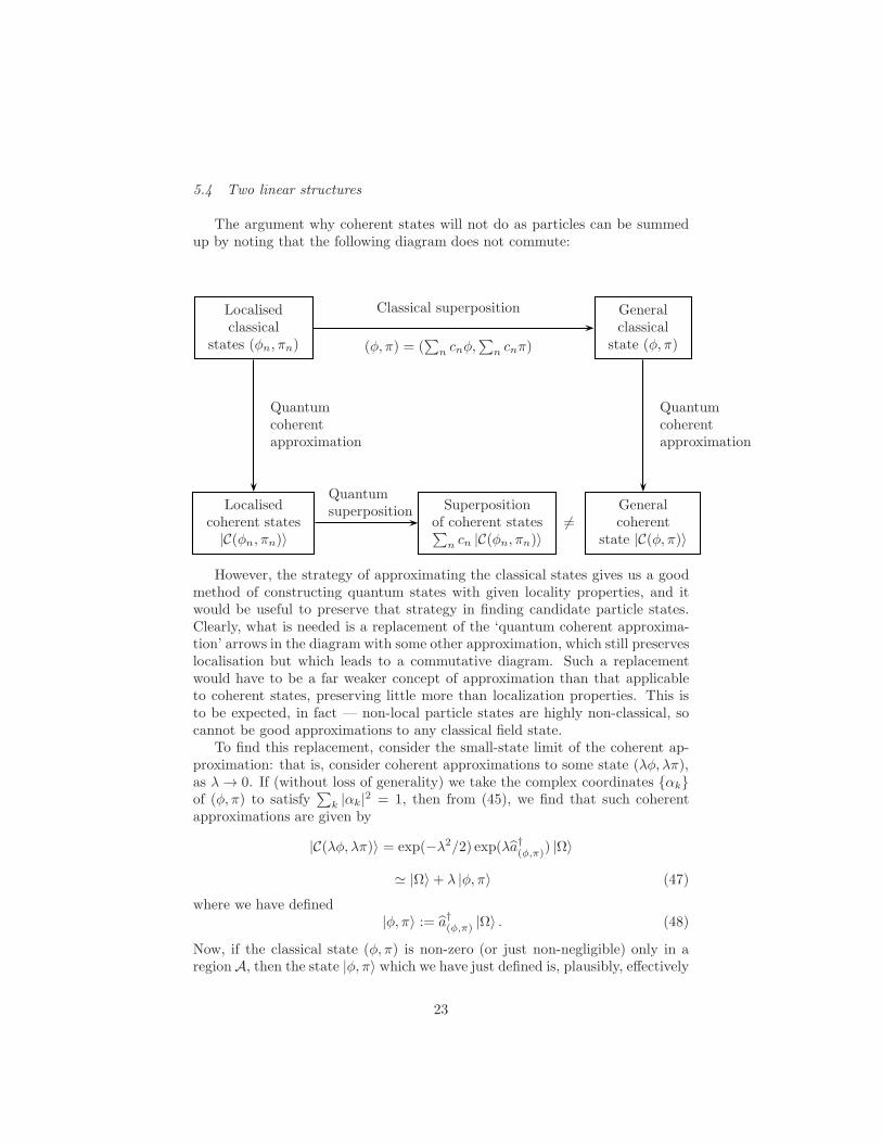
The argument why coherent states will not do as particles can be summedup by noting that the following diagram does not commute:

Localisedclassical

states (φn, πn)

Generalclassical

state (φ, π)

Localisedcoherent states|C(φn, πn)〉

Generalcoherent

state |C(φ, π)〉

Superpositionof coherent states∑

n cn |C(φn, πn)〉6=

Classical superposition

(φ, π) = (∑

n cnφ,∑

n cnπ)

Quantumsuperposition

Quantumcoherentapproximation

Quantumcoherentapproximation

However, the strategy of approximating the classical states gives us a goodmethod of constructing quantum states with given locality properties, and itwould be useful to preserve that strategy in finding candidate particle states.Clearly, what is needed is a replacement of the ‘quantum coherent approxima-tion’ arrows in the diagram with some other approximation, which still preserveslocalisation but which leads to a commutative diagram. Such a replacementwould have to be a far weaker concept of approximation than that applicableto coherent states, preserving little more than localization properties. This isto be expected, in fact — non-local particle states are highly non-classical, socannot be good approximations to any classical field state.

To find this replacement, consider the small-state limit of the coherent ap-proximation: that is, consider coherent approximations to some state (λφ, λπ),as λ→ 0. If (without loss of generality) we take the complex coordinates αkof (φ, π) to satisfy

∑k |αk|2 = 1, then from (45), we find that such coherent

approximations are given by

|C(λφ, λπ)〉 = exp(−λ2/2) exp(λa†(φ,π)) |Ω〉

≃ |Ω〉+ λ |φ, π〉 (47)

where we have defined|φ, π〉 := a†(φ,π) |Ω〉 . (48)

Now, if the classical state (φ, π) is non-zero (or just non-negligible) only in aregionA, then the state |φ, π〉 which we have just defined is, plausibly, effectively

23

localised in A: for it is a linear combination of |C(φ, π)〉 (which is a coherentapproximation to (φ, π), and thus presumably localised in A) and |Ω〉 (which,trivially, is localised everywhere).

Of course, plausibility is at the moment all we have: as section 3.1 explained,effective localization is not in general a linear property. But in the followingsection we will calculate the actual localization properties of |φ, π〉, and findthat they are indeed localized in the same region as the classical state. For themoment note that if such states are localised correctly then they are preciselywhat we are looking for — for if we define |k〉 = a†k |ω〉 :=

∣∣fk/√2ωk, 0

⟩, we

have (from 44) that

|φ, π〉 =∑

k

αk |k〉 . (49)

From this it follows immediately that the |φ, π〉 states form a subspace, and thatthe linear structure on that subspace mirrors the linear structure of the classicalstates being approximated:

a†(Aφ+A′φ′,Aπ+A′π′) = Aa†(φ,π) +A′a†(φ′,π′). (50)

5.5 Localization properties of |φ, π〉 states

To investigate the localisation properties of the |φ, π〉, we need to be able to

calculate the expectation values of products of φ(x) and π(x) operators, and themajor tool we shall use will be knowledge of the (easily-calculated) commutators

[φ(x), a†φ,π

]=

1

2

(φ(x) + i(R−1/2π)(x)

)(51)

and [π(x), a†φ,π

]=

1

2

(π(x) − i(R1/2φ)(x)

). (52)

With these known, we can calculate expectation values by the usual method ofmoving the annihilation operators over to the right where they annihilate |Ω〉.For instance:

〈φ, π| φ(x)2 |φ, π〉 ≡ 〈Ω| aφ,πφ(x)2a†φ,π |Ω〉 (53)

= 〈Ω| φ(x)φ(x) |Ω〉+ 2[φ(x), a†φ,π

] [φ(x), a†φ,π

]∗. (54)

Subtracting off the vacuum expectation value (which is in general divergent,hence depends on whatever high-energy cutoff procedure we have chosen touse), we get

〈φ, π| φ(x)2 |φ, π〉 − 〈Ω| φ(x)2 |Ω〉 = φ(x)2 + (R−1/2π)(x)2. (55)

In a similar way, we can calculate

〈φ, π| π(x)2 |φ, π〉 − 〈Ω| π(x)2 |Ω〉 = π(x)2 + (R1/2φ)(x)2, (56)

24

〈φ, π| 12π(x)2 +

1

2φ(x)

(Rφ)x) |φ, π〉 − 〈Ω| 1

2π(x)2 +

1

2φ(x)

(Rφ)x) |Ω〉

=1

2π2(x) +

1

2

(R1/2φ

)2(x), (57)

etc. (The last expectation value is that of the energy density, i. e. the (0, 0)component of the stress-energy tensor.) In each case — and, it is easy to see,for any such expectation value — the expectation value is some function of theclassical fields φ, π, modified by the action of some fractional power of R. (Inparticular, the energy density is equal to the classical energy density up to theaction of such operators.) Given that, at the end of section 4.2, R was requiredto satisfy either axiom 5b (which entails that all Rλ are Lc-local for some Lc)or axiom 5a (which requires this by fiat) it follows that

• If (φ, π) is localised in a region A then the difference of expectation valuesof |φ, π〉 falls off like exp(−d/Lc) with distance d from A.

• Hence, by the definition of effective localisation (in section 3.2), if (φ, π)is localised in a region A then |φ, π〉 is effectively localised in the sameregion.

• In view of the linearity of the map (φ, π) → |φ, π〉 which we have con-structed between classical and quantum states, it follows that the spaceof all states |φ, π〉 obeys ELP on scale Lc.

Note that (given the definition of Lc-localised states) any structure that theclassical state has on scales smaller than Lc is likely to be disrupted by theaction of Rλ; in particular, for a classical state (φ, π) localised in a region smallcompared with Lc, the corresponding quantum state |φ, π〉 will have little incommon with the classical state other than being effectively indistinguishablefrom the vacuum at distances from the classical state which are large comparedwith Lc.

5.6 Particles at last

Let us review the process we have used to construct the |φ, π〉 states. Wehave taken a classical wave-packet and constructed a coherent state around it.This state turns out to be expressible as the coherent state generated by asingle creation operator, and in turn the action of that creation operator on thevacuum produces a state which is localised in the same region as the classicalwave-packet (up to variations of size ∼ Lc).

It is now easy to see that the following diagram commutes:

25

Classicalwave-packet(φ(x), π(x))

Classicalmodesfk(x)

Quantumcoherent state

D(φ,π) |Ω〉

Quantumcoherent modes

Dk |Ω〉

Localisedparticle state

|φ, π〉 = a†(φ,π) |Ω〉

Particlemomentumeigenstates

|k〉 = a†k |Ω〉

Classical superposition

φ(x) =∑

k1√2ωk

(αkfk(x) + α∗kf

∗k (x))

π(x) = i∑

k

√2ωk (αkfk(x) − α∗

kf∗k (x))

Quantum combination

D(φ,π) |Ω〉 =∏

k Dk(αk) |Ω〉

Quantum superposition

|φ, π〉 =∑k αk |k〉

Coherentquantumapproximation

Coherentquantumapproximation

Restrict toaction offirst-ordercomponent

of Dk

Restrict toaction offirst-ordercomponent

of D(φ,π)

The important properties of the diagram are:

1. Moving down the diagram preserves Lc-localisation properties.

2. Moving from the first to the second row takes us from the classical to thequantum regime, but does not drastically change the nature of the states:states in the second row are good approximations of those in the first row,in the sense spelled out in sections 5.1–5.2 This is not true for the thirdrow: the only sense in which |φ, π〉 approximates (φ, π) is that they sharethe same localisation properties.

3. Moving leftward across the diagram corresponds to the combination ofmodes to make localised states. The middle (dashed) line is not a linearprocess, but the top and bottom lines both represent linear superposition.However, though mathematically very similar, these superpositions havephysically very different meanings.

4. In the quantum superposition process, it is natural to consider complexweightings for the states being superposed. The (mathematically) equiva-lent process at the classical level provides a generalisation of the real-linear

26

superposition process for classical states, effectively equipping the classicalsolution space with a complex structure (of which more later).

With these results in hand, it is easy to verify that the space of |φ, π〉 statesis indeed a one-particle space in the sense of section 3.2. The localised statesare constructed by beginning with classically localised wave-packets and movingdown the diagram. The requirement that all states in the space are superpo-sitions of localised ones follows from the equivalent property of classical phasespace together with the commutativity of the diagram. The validity of the su-perposition principle among effectively localised states is a trivial consequenceof the diagram’s commutativity. And, crucially, the closure of the one-particlesubspace under time-evolution follows once we observe that the |k〉 are energyeigenstates: this means that the projection operator onto the one-particle sub-space commutes with the Hamiltonian, so the subspace must be preserved undertime evolution. (Equivalently, closure under time evolution follows once we ob-serve that the map

(φ, π) −→ |φ, π〉 (58)

commutes with time evolution.)The essential property of the QFT which makes this whole process possible is

its linearity: without the linearity, we would not have the classical linear struc-ture whose interplay with the linear structure of HΣ allowed our constructionto proceed.

Henceforth, we will denote the space of all |φ, π〉 by H1P .

6 Development of the particle concept

In this section we will analyse further the construction of particles presentedabove. We will examine the importance of the Compton wavelength, and de-velop the links between the linear structures on phase space and on Hilbertspace; we will then use this analysis to give an alternative way of constructingthe one-particle subspace.

6.1 Significance of the Compton wavelength

The results above imply that it is localisation on the scale of the Comptonwavelength Lc, and not exact localisation, that is significant for particles. Thereis a straightforward physical reason for the significance of Lc: as mentioned insection 3.1, the vacuum state of any QFT is entangled (in the sense that fieldstates in different spatial regions are entangled) and this entanglement cannotbe removed from the non-vacuum states of the field without interfering with thefield’s structure at energy levels comparable to the cutoff energy (in other words,without going beyond the domain of validity of QFT). However, the correlationsin the vacuum drop off with spatial distance, as can be seen from calculatingquantities such as

27

〈Ω| φ(x)φ(y) |Ω〉 − 〈Ω| φ(x) |Ω〉 〈Ω| φ(y) |Ω〉

=1

2R−1/2δ(x− y). (59)

If R−1/2 is non-local on lengthscales of ∼ Lc, then we can treat spatial regionsseparated by distances large compared with Lc as uncorrelated, but it makesrather little sense to talk about localisation on scales small compared with Lc.

This also gives us at least heuristic grounds to extend the concept of theCompton wavelength beyond Euclidean-invariant R. As was shown in section4.1, the locality of R requires it to have form

(Rf)(x) =∑

|α|≤N

cα(x)Dαf(x), (60)

with Euclidean-invariant R corresponding to each cα being constant. Now, ifwe start with such a Euclidean-invariant R and introduce a very slow variationin its cα (with ‘very slow’ meaning ‘significant variation on lengthscales muchlonger than the Compton wavelength’), then we would expect the vacuum entan-glement lengthscale to remain substantially unchanged, which in turn suggeststhat R−1/2 would remain non-local on the same lengthscales.

Of course, we are using physical intuition to conjecture results of a math-ematical nature, and this conjecture is ultimately no substitute for rigorousresults about the operators R−1/2 in the non-Euclidean-invariant case.

6.2 Field-particle duality

The map(φ, π) −→ |φ, π〉 (61)

defines a vector-space isomorphism9 between H1P and the classical phase spaceP ; since it commutes with time evolution, it also defines an isomorphism betweenH1P and the classical solution space. We can use this isomorphism to pullback the Hilbert-space structure (i. e. , the complex structure and the innerproduct) from H1P to phase space, and hence to solution space: thus, we gaina prescription by which we can regard P as a Hilbert space.10

It is instructive to give the precise forms for the complex structure (i. e. ,the linear operator J corresponding to multiplication by i) and inner product〈〈 , 〉〉. on P . We will express each in three ways:

9Strictly speaking the map takes phase space only into a proper subset of H1P , becausethe image of the map is not complete in the Hilbert-space norm on by the latter (induced fromHΣ). Our relaxed attitude to this is due to our approach (in section 2.3) to renormalisation: wewill regard H1P as being cut off at some (very high) energy, thus making it finite-dimensionaland removing the problem.

10The existence of a complex structure on the classical phase space has long been known,and in fact is a central part of Segal’s (1964) approach to quantisation (briefly discussed insection 8.2).

28

1. In terms of qk and pk:

J(q1, p1; . . . ; qk, pk; . . .) = (−p1, q1; . . . ;−pk, qk; . . .);

〈〈 (φ, π), (φ′, π′) 〉〉 = 1

2

∑

k

[(qkq′k + pkp

′k) + i(qkp

′k − pkq′k)]. (62)

2. In terms of αk:

J(α1, . . . , αk, . . .) = (iα1, . . . , iαk, . . .);

〈〈 (φ, π), (φ′, π′) 〉〉 =∑

k

α∗kα

′k. (63)

3. Directly in terms of (φ, π):

J(φ, π) = (−R−1/2π,R1/2φ);

〈〈 (φ, π), (φ′, π′) 〉〉 = 1

2

∫

Sd3x

(φ(x)R1/2φ′(x) + π(x)R−1/2π′(x)

)

+i

2

∫

Sd3x (π(x)φ′(x) − φ(x)π′(x)) , (64)

or

〈〈 (φ, π), (φ′, π′) 〉〉 = 〈R1/4φ+ iR−1/4π,R1/4φ′ + iR−1/4π′〉 (65)

where 〈 , 〉 is the ordinary L2 inner product on S.From (2) it is easy to confirm that J and 〈〈 , 〉〉 are preserved by time-evolution.The fractional powers of R which occur in (3) tell us that J and 〈〈 , 〉〉 are notstrictly local.

Since H1P and P are isomorphic, we can use this Hilbert-space descrip-tion of P to provide a coordinatisation of H1P itself. This gives us a sort ofwave-function description, albeit one in which the complex structure and innerproduct are not locally defined. Such a description is an expression, in a sense, ofwave-particle duality, with the same mathematical description applicable to theone-particle subspace of the quantum system, and to the whole classical system.Note, though, that the duality is critically dependent upon the linear structureof the solution space — hence we have no reason to regard field-particle dualityas a general property of field theories, but only of linear (or nearly linear) ones.

The duality also implies that dynamics on phase space must be writeable inSchrodinger-equation form. Indeed, it is straightforward to check that Hamil-ton’s equations

φ = π; π = −Rφ (66)

are equivalent tod

dt(φ, π) = −JR1/2(φ, π), (67)

so that the Hamiltonian is the (mildly nonlocal) operator R1/2.

29

6.3 Alternative construction of particles: heuristic form

We have argued that it is the interplay between two Hilbert-space structures— the quantum-mechanical one and the one on the classical solution space —which leads to the emergence of particles, but it is perhaps somewhat obscureexactly how that interplay comes about. In this section and the next we willdescribe an alternative way to the particle subspace which possibly gives moreinsight into this question.

The basis of our new method is as follows: since the vacuum is significantlyentangled only on lengthscales of order the Compton wavelength, we wouldexpect that the action of a field observable like φ(x) on the vacuum wouldcreate a state differing from the vacuum only in the vicinity of x — that is,a state Lc-localised at x. We might further expect that, if f and g are realfunctions which vanish outside some spatial region Σ1, then the state

∫d3x

(f(x)φ(x) + g(x)π(x)

)|Ω〉 (68)

would be Lc-localised in Σ1. Furthermore, the space of all such states (68) is

spanned by states of form φ(x) |Ω〉 and π(x) |Ω〉 — that is, by states which weexpect to be Lc-localised at a point.

It should be stressed that it is by no means obvious that these ‘expectations’will be confirmed: the Reeh-Schlieder theorem reminds us that the link betweenthe localisation properties of operators and of those states created by the actionof those operators on the vacuum is rather subtle. Nonetheless, if they areconfirmed then the space of states of the form (68) satisfies our first two criteria(on page 12) for a particle subspace: that the ELP holds for the space, and thatthe space is spanned by a basis of localised states. (And in fact they can beconfirmed.)

No use has yet been made of the linearity of the classical solution space,so it is perhaps unsurprising that this property is essential to (amongst otherthings) ensure that our space is to satisfy the third criterion for a one-particlespace: that the space is at least approximately preserved under time evolution.For the linearity of the classical field equations is equivalent to the requirementthat the Hamiltonian is quadratic in the fields and their conjugate momentum,and this in turn entails that (writing U(t) = exp(−iHt) for the time-translationoperator),

U(t)φ(x)U†(t) ≡ φ(x)− it

[H, φ(x)

]− t2

[H,[H, φ(x)

]]+ . . . (69)

is a linear combination of φ and π operators — hence, the time evolution ofa state like φ(x) |Ω〉 is a state of form (68). This clearly entails the closure ofthe space of states of form (68) under time-evolution; hence, it is a one-particlespace.

30

6.4 Alternative construction of particles: technical details

Let us develop the formal details of this sketch. We begin in classical me-chanics: recall that a classical observable is a real functional on the phase space(so in one-particle mechanics the position observable assigns to each phase-spacepoint its configuration-space position, etc.) It will be important to preserve, inthe following, the distinction between the phase-space point (φ, π), which is astate of the classical field, and the classical observables φ(x) and π(x), whichare functionals on the space of field states: the action of φ(x) on a field statereturns the field strength at the point x.11 To make this distinction clear, inthis section we will distinguish classical observables by writing them with a baron top of them: φ(x), for instance. Thus, the observables φ(x) and π(x) aredefined by

φ(x)[(φ, π)] = φ(x) (70)

andπ(x)[(φ, π)] = π(x). (71)

The space of observables in any classical-mechanical system has a naturallinear structure: (A + B)[v] := A[v] + B[v]. Furthermore, we can define timeevolution for observables as follows: if, for any phase-space point v, v(t) denoteswhere that phase-space point has moved to after time t, then we define

A(t)[v] := A[v(t)]. (72)

If H is the classical Hamiltonian then we can write A(t) in the symbolic form

A(t) = exp(−tH, ·

)A, (73)

(which is to be understood as denoting the power-series expansion

A(t) =

( ∞∑

n=0

(−t)nn!

H, ·

)A (74)

whereH, ·

A :=

H,A

.) This movement of the dynamics from the states to

the observables is very similar, both conceptually and mathematically, to themove from the Schrodinger to the Heisenberg picture in quantum mechanics. Itis discussed in more detail by Woodhouse (1991, p.20 et seq. ).

Although we generally regard observables as real functionals, there is nothingto prevent us expanding the class of observables to include complex functionals,and we shall do so from here on. Any complex observable, of course, has theform A+ iB, where A and B are real observables.

So far, everything we have said about observables applies to any classicalsystem. If, however (as in the case of linear field theory) the classical phasespace has a linear structure which is preserved under time evolution, then it

11Similarly, in particle mechanics there is a distinction between a particle’s position x andthe observables x

i, which are functionals returning the ith component of a particle’s position.

31

is possible to define real-linear observables as those real observables which arereal-linear functionals; since the linear structure commutes with time evolutionon phase space then it is easy to verify that it commutes with time evolutionon the space of linear observables as well. In the specific case of classical fields,the linear observables are precisely those of form

∫

Σ

d3x(f(x)φ(x) + g(x)π(x)

)(75)

with f and g real functions. We will refer to any such observable as Lc-localisedin a region Σ1 if the functions f and g are Lc-localised in that region.

Since, as we have seen (in section 6.2), the classical phase space can begiven the structure of a complex Hilbert space,12 we can also define complex,conjugate-linear observables in the obvious way (i. e. all those complex observ-ables which are real-linear and which satisfy C[J(φ, π)] = −iC[(φ, π)].) It iseasy to see that each such observable can be written as C = A + iB, with Aand B real-linear observables.

Now, it is a basic result of Hilbert space theory (the Riesz representationtheorem) that the space of conjugate-linear functionals on a Hilbert space isisomorphic to that Hilbert space: in other words, that to each conjugate-linearfunctional Λ there corresponds a unique vector u such that, for any v, Λ[v] =〈u,v〉. Hence, the space of complex conjugate-linear observables over the phasespace of a classical linear field, conceived as a Hilbert space, is Hilbert-space-isomorphic to the phase space itself. This isomorphism takes the somewhatawkward form

(φ, π)←→∫

Σ

d3x((R1/2φ(x)− iπ(x))φ(x) + (R−1/2π(x) + iφ(x))π(x)

)

(76)from which we can see that it preserves Lc-locality. It takes a far simpler form(albeit one in which its locality is obscured) if we use the αk coordinates for(φ, π): if we define the observable a∗k by a∗k[α1, . . . αn, . . .] := αk then theisomorphism is

α1, . . . αn, . . . ←→∑

k

αka∗k. (77)

The move from classical to quantum mechanics can be thought of as analgorithm taking classical observables to quantum operators; it cannot be ap-plied to all observables but in field theory it does apply to all of the real-linearobservables, being generated by the maps

φ(x) −→ φ(x) (78)

andπ(x) −→ π(x). (79)

12As was mentioned briefly before (in footnote 9 on page 28) this is strictly correct only ifwe complete the classical phase space in the norm generated by its inner product.

32

The quantization map is linear, commutes with time evolution, preserves locality(trivially) and can be extended to complex conjugate-linear observables in the

obvious way: A+ iB −→ A+ iB. As might be expected, it can be written as

∑

k

αka∗k −→

∑

k

αka†k. (80)

We have now moved from classical states, to classical observables, to quan-tum observables. Finally, we move to quantum states by applying the appro-priate quantum observable to the vacuum state |Ω〉. If the vacuum is entangledon lengthscales of Lc, then we expect (though it is not a priori guaranteed) thatthis map, too, is Lc-local.

This sequence of three linear isomorphisms, each commuting with time evo-lution, can be summarised in the following diagram.

Classicalstate

(φ, π) ≃α1, . . . , αn, . . .

Classicalstate

(φ(t), π(t)) ≃. . . , αne

−iωnt, . . .

Classicalobservable∑

k αka∗k

Classicalobservable∑k αke

−iωkta∗k

Quantumoperator∑

k αka†k

Quantumoperator∑k αke

−iωkta†k

Quantumparticle∑k αka

†k |Ω〉

Quantumparticle∑

k αke−iωkta†k |Ω〉

Time evolution

via Hamilton’s equations

Time evolution

via A = −H,A

Unitary time-evolution

(Heisenberg picture)

Unitary time-evolution

(Schrodinger picture)

Isomorphismbetween statesand functionals

Isomorphismbetween statesand functionals

Quantization Quantization

Apply tovacuum

Apply tovacuum

The important properties of the diagram are:

33

• Each map on the diagram is linear; hence, the linear structure on classicalphase space transfers to the one-particle subspace.

• Nonetheless, the linear structures mean very different things: the lin-ear structures on the classical and quantum observables are conceptuallyclosely related to one another, but are conceptually different from the lin-ear structure on the classical phase space, which in turn is conceptuallydifferent from the linear structure on the one-particle space.

• The vertical maps preserve Lc-localization; hence the one particle subspacesatisfies the effective localisation principle on scale Lc and is spanned bystates which are Lc-localised at a point. (This is true by definition betweenthe first and second lines (cf. page 32), and trivial to show between thesecond and third lines. The substantive step is the one between the thirdand fourth lines — between quantum operators and quantum steps. Itis made plausible by the observations of section 6.1 (that the vacuum issignificantly entangled only on lengthscales of ∼ Lc), and proved by thecalculations of section 5.5.)

• The diagram commutes; in other words, time evolution commutes witheach horizontal map. This ensures that states within the one-particle sub-space remain in that space, i. e. that particle states are taken to particlestates under time evolution.

Compared with the coherent-states method used earlier to construct parti-cles, this new method has the advantage of showing more clearly how the linearstructure transfers from classical to quantum states; however, it provides muchweaker reasons for believing that the map between classical and quantum statespreserves Lc-locality.

(Of course, even in the coherent-state method, the argument given for parti-cle locality was only heuristic, relying on the assumption that if |C〉 is a coherentstate Lc-localised in some region, then |C〉 − |Ω〉 is Lc-localised in the same re-gion. Ultimately, the only way to check Lc-locality is by direct calculation.)

7 The Newton-Wigner representation of H1P

In this section, we will consider the so-called ‘Newton-Wigner’ definition oflocal states, which we will generalise from Lorentz-invariant QFTs to the linearQFTs discussed above.

7.1 Mathematical argument for the Newton-Wigner representation

Although the representation of H1P given in the previous section is a sortof configuration-space representation, it is somewhat awkward to use comparedto the configuration-space representations which we are accustomed to in non-relativistic quantum mechanics — essentially because of the non-local nature ofthe inner product and complex structure.

34

Purely for mathematical convenience, it would be useful to find a way oftransforming our current representation into one where the inner product andcomplex structure are represented as local operations — such a transformationwould inevitably have to be nonlocal itself, but since we realise that the particlestates are unavoidably mildly nonlocal (on scales of Lc) this is not problematic.Finding such a transformation is straightforward: it is given by

(φ, π)→R1/4φ− iR−1/4π, (81)

or, in terms of the αk coefficients, by

|φ, π〉 =∑

k

αk |k〉 →∑

k

αkfk(x). (82)

It is straightforward to verify that in the new representation, the complex struc-ture is just multiplication by i and the inner product is the usual L2-product.Unless (φ, π) is localised in a region small compared with Lc then its locali-sation will not be significantly changed by the transformation; hence, the newrepresentation is an equally accurate representation of the actual localisationproperties of the quantum states. In the case of Klein-Gordon theory, this isknown as the Newton-Wigner representation (Newton and Wigner 1949) and wewill adopt this nomenclature for all such representations (i. e. , including QFTsother than Klein-Gordon theory).

If we denote the transformation from the phase-space representation of H1P

to the Newton-Wigner representation by N , then its complex-linearity is equiv-alent to the statement

iN = NJ. (83)

Applying N to both sides of the Schrodinger equation (67), we get

d

dtN (φ, π) = −NJR1/2(φ, π) = −iR1/2N (φ, π) (84)

so that the Hamiltonian in the Newton-Wigner representation is again R1/2.In the specific case of Klein-Gordon theory, we have R1/2 = (m2 −∇2)1/2, andin the non-relativistic limit this is approximately equal to m−∇2/2m, so thatwe recover the non-relativistic free-particle Hamiltonian (up to an additive con-stant, the rest energy of the particle). It might appear that we have replaced anonlocal operator with a local one, but for the nonrelativistic approximation tobe valid we require that the wave-function contains only a negligible contribu-tion from eigenstates which don’t satisfy |k| ≪ m — which in turn means thatit must be localised in a region of size ≫ Lc.

7.2 Conceptual significance of the Newton-Wigner representation

There is another way to motivate the Newton-Wigner representation, basedmore on conceptual than mathematical grounds. In Dirac’s formulation of non-relativistic quantum mechanics, the configuration space wave-function is intro-duced by

ψ(x) ≡ 〈x|ψ〉 , (85)

35

where the states |x〉 are the eigenstates of the position operator — so that theintegral of the wave-function over a small region gives the amplitude for theparticle to be in that region. This fits well with our description of a one-particlespace in section 3.2 as a subspace spanned by well-localised states (indeed, in thenon-relativistic case such states can be arbitrarily well localised) and it wouldbe useful to have a similar representation of QFT particles.

To what extent does the Newton-Wigner representation provide this? Thedelta functions are certainly formally equivalent to position eigenstates, beingperfectly localised in configuration space and forming an (improper) basis forthe one-particle Hilbert space. But obviously they are not precisely localised inreal space: if |xNW 〉 is the abstract ket corresponding to a delta-function at X,then we have

|xNW 〉 =∑

k

f∗k (x) |k〉 , (86)

and it is easy to verify that (for instance)

〈xNW | φ(y)φ(y) |xNW 〉 − 〈Ω| φ(y)φ(y) |Ω〉 (87)

is formally equal to1

2

[R1/4δ(x− y)

]2, (88)

and hence is localised only within a region of size ∼ Lc.This is not a problem, however. Recall that even in non-relativistic quantum

mechanics, no particle can actually be placed in an eigenstate of position (suchstates are not even in Hilbert space). Rather, such states are to be seen asan idealised mathematical limit of a sequence of successively better-localisedstates (see, e. g. , Cohen-Tannoudji, Diu, and Laloe (1977, pp. 100–105)). Wecan apply the same approach here, with the proviso that the successive terms ofthis sequence are only successively better localised in physical space (as opposedto in Newton-Wigner configuration space) up to a point: the point at which theterms are localised in regions which are not large in comparison with Lc. Afterthat point the states will remain localised in a region of size ∼ Lc irrespectiveof how localised the Newton-Wigner wavefunction is. But providing that thewavefunctions which we are studying do not themselves vary on lengthscalescomparable to Lc, we will only need those terms in the sequence which are largecompared with Lc — hence, we may effectively use the concept of ‘positioneigenstate’.

Providing the Newton-Wigner wavefunction varies slowly on lengthscales ofsize Lc, we can regard the integral of the function over regions of this size asgiving the amplitude to find it in a state effectively localised in the region. Thisthen allows us to define an effective position operator:

XNW ≡∫

Σ

d3x |xNW 〉 〈xNW | . (89)

This operator will perform the same task as the non-relativistic position op-erator, provided that we are not interested on scales small compared with the

36

minimum localisation scale: its expectation value will give the expected value ofthe particle’s position upon measurement, and projections built from its spec-trum correspond to projections onto the particle being in a given region (alwaysassuming that region to be large compared with the minimum localisation scaleLc).

However, the relationship between this position operator and the Newton-Wigner position states is opposite from that which holds between non-relativisticposition operators and position eigenstates (at least in some presentations). Inthe latter case, the position operator is our starting point and position eigen-states are position eigenstates because they are eigenstates of the position op-erator. In QFT, the Newton-Wigner position states are approximately localbecause of their relationship with the field observables, and the position opera-tor is constructed from them.

7.3 “Pathological” features of the Newton-Wigner representation

The Newton-Wigner representation of Klein-Gordon particles is well knownto have two apparently pathological features: eigenstates of position do not re-main eigenstates under Lorentz transformations, and Newton-Wigner wavefunc-tions spread out superluminally. From the current perspective, both propertiesare curiosities rather than pathologies. The Newton- Wigner representation isnot covariantly defined, so there is no mathematical reason to expect localisa-tion to be totally unaffected by Lorentz boosts — but the boosts do not causeone-particle states which are effectively localised in a given region to stop beinglocalised in that region. Similarly, Newton-Wigner wave-functions do spreadfaster than light — but the transformation between phase space P and theNewton-Wigner representation commutes with time evolution, so the Newton-Wigner state continues to represent a state effectively localised in the regionoccupied by a classical state which is propagating at subluminal speeds.

As such, the Newton-Wigner representation is a perfectly legitimate, andoften very convenient, way of describing states in the one-particle subspace— but it doesn’t give the exact truth of the matter as to where particles arelocalised, because there isn’t one: particles are superpositions of field excitationswith finite size, so any attempt to give a wave-function description down toarbitrarily small scales is inevitably going to be itself arbitrary at those scales.

Before ending this discussion, I should note that there is an alternative tradi-tion (going back to (Segal 1964), and currently defended by Fleming (1996)) thattakes Newton-Wigner-localised states as by definition localised. In this view-point, localisation of states is defined directly in terms of the Newton-Wignerposition operator, rather than (as here) via the localisation properties of theoperator algebra. Such an approach, by taking the Newton-Wigner position op-erator as having fundamental significance, must of course confront the apparentpathologies of the Newton-Wigner representation.

This paper, however, has as a starting assumption that localisation is definedvia the operator algebra, and as such I will not discuss Fleming’s approach. Thereader interested in how (and if) the alternative tradition can come to terms

37

with the pathologies should see Fleming and Butterfield (1999) as well as therecent exchange of views between Fleming (2000) and Halvorson (2001).

8 Comparisons with other methods

This section is a brief comparison of the results of this paper with twoother approaches to quantum field theory: the collision theory developed inthe framework of algebraic QFT by Haag and Ruelle, and Segal’s approach toquantizing linear systems.

8.1 Comparison with Haag-Ruelle collision theory

Haag-Ruelle theory (discussed in Haag (1996), and references therein) is ananalysis of collision theory, and of the particle content of quantum fields, withinthe framework of algebraic QFT. Conceptually speaking this is essentially thesame framework used here (although treated with significantly more mathemat-ical care13): the field is taken as primary and particles are regarded as emergentconcepts; thus, this paper’s approach is complementary to, and not in conflictwith, Haag-Ruelle theory.

A detailed description of the theory lies beyond the scope of this paper,but essentially it applies to any Poincare-invariant QFT which has a discreteeigenvalue of the mass observable (other than zero) and for which the massspectrum of the subspace orthogonal to the vacuum has a lower bound awayfrom zero (so that it implies, for instance to massive Klein-Gordon theory). Andit establishes that at asymptotically early and late times,

1. The QFT behaves as a free, massive QFT;

2. Any state which lies in the N -particle sector of that free theory can setoff at most N widely separated detectors.

Note that the theory applies to interacting as well as to free theories; how-ever, it only applies at asymptotically early and late times, and implies that anyQFT is effectively free at such times; thus, it entails a particle interpretationonly for effectively free fields (which is the case described above). Its virtue overthe approach of this paper is its generality (it applies to fermionic as well asbosonic fields, and to composite as well as ‘elementary’ particles) and its abil-ity to infer the particle properties of the field directly from its mass spectrum,without recourse to concepts of field-particle duality. However, for this veryreason the close relationship between classical solutions and one-particle statesis somewhat obscure in the Haag-Ruelle analysis.

At first sight, the generality of the Haag-Ruelle analysis might seem to under-mine the argument of section 6.2 that the particle concept is essentially boundup with the linearity of the field theory in question. However, the analysis itselftells us that the existence of a massive asymptotic limit of a field theory, and

13See Wallace (2001b) for a discussion of the relationship between algebraic QFT and theprima facie less rigorous QFT described here and used in mainstream physics.

38

the existence of a discrete nonzero mass, are really equivalent statements. Inthe context of the present paper, the Haag-Ruelle analysis should remind usthat the linear theories we are studying should be regarded as effective, asymp-totic limits of interacting field theories, and not as fundamental fields in theirown right: for instance (though technically it lies rather beyond the scope ofthis paper since it deals with fermionic particles) we would expect QCD to beasymptotically analysable in terms of ‘proton’ and ‘neutron’ fields, but thesebear little resemblance to the fundamental — and strongly interacting — quarkfields of QCD.

(Technically, the analysis of this paper might seem more general than theHaag-Ruelle theory since the latter is confined to Poincare-invariant QFTs.However, we can extend Haag-Ruelle theory to general translation-invariantQFTs by generalising its spectral condition to require that the 4-momentumspectrum includes a discrete surface in 4-momentum space which nowhere in-tersects the origin (we get this for free by Lorentz invariance in a relativistictheory, once we have specified a discrete mass eigenstate). It is at best unclearhow to apply Haag-Ruelle theory to QFTs without translational symmetry; itshould, though, be acknowledged that the above analysis is also not entirely sat-isfactory in such situations as we have only a heuristic argument for the approx-imate locality of non-translation-invariantRλ operators — recall the discussionof section 6.1.)

8.2 Comparison with Segal quantization

It is instructive to compare the field-quantization approach given above withthe quantization program developed by Segal (1964) and others (see Saunders(1992) for a foundational discussion). In Segal’s approach, we begin by choosinga complex structure J on the phase space of a linear field,14 which we require tohave certain properties (specifically, for any states u, v, we require J to satisfyΩ(Ju, Jv) = Ω(u, v), and Ω(Ju, u) ≥ 0, where Ω(·, ·) is the symplectic form onP). We then use J to define an inner product on P , given by

〈〈u, v 〉〉 ≡ Ω(Ju, v)− iΩ(u, v). (90)

This (following norm-completion) makesP into a Hilbert space (the ‘one-particleHilbert space’), on which we can easily show that the classical dynamics areunitary. The Fock space generated from that Hilbert space is then taken to bethe Hilbert space of the QFT, and there is a very natural definition of the actionof the field operators upon that space.

This is effectively the reverse procedure to ours. In Segal’s approach, webegin with the Hilbert-space structure on phase-space, declare it to be the one-

14 There is another approach very closely related to Segal quantization, in which insteadof choosing a complex structure, we complexify the phase space and then choose a subspaceof (formally) half the dimension of the complexified phase space. This process is at least for-mally equivalent to choosing a complex structure, though there are some infinite-dimensionaltechnicalities to take care of: see Wald (1994) for an exposition of this method, and especiallyp. 46 of his book for the relationship with the Segal method.

39

particle Hilbert space, and then build the full QFT Hilbert space HΣ from thatstructure; in ours, we begin with HΣ, identify a subspace which deserves to becalled the ‘one-particle’ space, and then use it to give a Hilbert-space structureto P .

This highlights an important conceptual difference between Segal quantiza-tion and the ‘canonical’ method of quantization used here. In our approach, themethod used to quantize a (bosonic) field theory is essentially the same irrespec-tive of whether that theory is linear: throw the theory into Hamiltonian formand look for a map from field observables to operators on some Hilbert space,such that Poisson brackets become commutators. Then if the classical theoryis linear, analysis of the quantum theory reveals the one-particle subspace. InSegal’s approach, on the other hand, the linearity is fundamental to the entirequantization algorithm, and it is most unclear how nonlinear field theories areto be accommodated.

The attitude which one may take towards this difference depends on one’sconfidence in the mathematical and conceptual status of nonlinear QFTs —in particular, the status of the infinities which arise in the dynamics of suchtheories, and of the renormalisation process used to tame them. If (with theauthor; see Wallace 2001b) one takes a relaxed attitude to these infinities, thenthe Segal process becomes an elegant curiosity: a nice way to understand linearquantization, but of little relevance to general QFTs. If, on the other hand,one regards the infinities as a pathological problem in QFT, then (as Saunders(1992) has argued) it may be a virtue of the Segal approach that it forces usto look for radical ways of reformulating the quantization of nonlinear fieldtheories.

It is also possible to see Segal quantization as pointing to a different viewof the relationship between field and particle than the one defended here. Asmentioned above, in Segal quantization it is necessary to begin by choosing acomplex structure on the classical phase space, and different choices of structurelead to one-particle spaces with different properties. If one believes that thereis a ‘right’ choice of complex structure, then there is also a ‘right’ one-particlespace, and that space is a fundamental building block when assembling the fieldHilbert space; this is at least suggestive of a more even relationship betweenfield and particle concepts than the field-is-primary viewpoint advocated above.

On the other hand, it is also reasonable to regard the choice of a complexstructure as just being a matter of taste, in which case the importance of theone-particle subspace is downgraded. One argument in favour of this attitudeis that in general it is very unclear what rule could pick out the ‘right’ complexstructure: there is a unique prescription in the case of a time-independent linearQFT (this includes the QFTs considered above) but in, say, the presence of atime-dependent potential, or in a curved spacetime, then there does not appearto be any general rule by which one complex structure could be preferred overanother. This is, of course, a variant of the last of the arguments which (insection 2.4) led us to regard field as primary in the first place.

40

9 Conclusion

We have shown that the one-particle subspace of a free, bosonic, massivequantum field emerges very naturally as a consequence of that field’s classicallinearity, and that the interplay between classical and quantum linear structuresis such as to give those particle states the right sort of locality properties.

It is important to remember that this sort of construction of particle spacesis not intended to be any sort of explanation as to why the world around us isobserved to be particulate. At best it is able to show how such observations arecompatible with the validity of QFT — the question of why the actual worldappears to be in a particulate state is much subtler. It presumably requiresconsideration of decoherence theory (see Anglin and Zurek (1996) for some ideasalong these lines), and more generally it involves the measurement problem.

It is also important to keep in mind the limitations on our construction. Al-though these results should extend straightforwardly to multi-component fields,they do not apply to the important cases of fermionic, and massless, fields. Inthe former case we would expect the particle concept to be more, not less, impor-tant, due to the Pauli exclusion principle; but the fact that spacelike-separatedFermi field operators anticommute rather than commute suggests that we canno longer visualise the QFT Hilbert space in terms of wave-functionals on con-figuration space. In the case of massless fields, we expect the particle concept tobe much more subtle:15 QED, for instance, possesses not only regimes in whichthe electromagnetic field is analyzable in terms of free photons, but regimes inwhich it should be thought of as a classical field, and others in which it simplyprovides a long-range force between nonrelativistic particles.

This brings up perhaps the most substantial limitation of this paper’s ap-proach to particles — and indeed of any approach which analyses particles interms of asymptotic behaviour. Although it may well be the case that there isno particulate description of high-energy phenomena except at asymptoticallyearly and late times, atomic and solid-state physics — not to mention biologyand chemistry — provide us with a wealth of situations in which ‘particles’(specifically, electrons and atomic nuclei) are strongly interacting and yet stillmaintain their own particle character. Analysing this situation would require adeep understanding of the nonrelativistic limit of massive and massless QFTs,and lies far beyond this paper’s scope.

Nonetheless, despite the limitations of this approach it is satisfying to findthat field-particle duality can be understood in the context of a field ontology,and intriguing to observe the elegant and somewhat subtle ways in which thevarious linear and complex structures present intertwine to make this under-standing possible.

Acknowledgements— I would like to thank Simon Saunders, whose own work on the

foundations of QFT prompted my interest in the subject; and Jeremy Butterfield for

15This is supported by the situation in algebraic QFT, in which development of a satisfactorycollision theory for fields without a mass gap is at a much more rudimentary stage; see Haag(1996) and Buchholz (2000) for recent discussions.

41

many useful comments on earlier drafts of this paper. I have also benefitted greatly

from conversations with Ian Aitchison, James Binney, Katherine Brading, Harvey

Brown, Keith Burnett, Peter Morgan, and Andrew Steane.

References

Anglin, J. and W. H. Zurek (1996). Decoherence of quantum fields: Pointerstates and predictability. Physical Review D 53 (12), 7327–7335.

Buchholz, D. (2000). Algebraic quantum field theory: a status report.Plenary talk given at the XIIIth International Conference on Mathe-matical Physics, London. Available online at http://xxx.arxiv.org/math-ph/0011044.

Clifton, R. and H. Halvorson (2001). Entanglement and open systems in alge-braic quantum field theory. Studies in the History and Philosophy of Mod-ern Physics 32, 1–31. Available online at http://xxx.arXiv.org/abs/quant-ph/0001107.

Cohen-Tannoudji, C., B. Diu, and F. Laloe (1977). Quantum Mechanics. NewYork: Wiley.

Coleman, S. (1985). Aspects of Symmetry: selected Erice lectures. Cambridge:Cambridge University Press.

Fleming, G. (1996). Just how radical is hyperplane dependence? In R. Clifton(Ed.), Perspectives on Quantum Reality, pp. 11–28. Dordrecht: KluwerAcademic Publishers.

Fleming, G. (2000). Reeh-Schlieder meets Newton-Wigner. Philosophy of Sci-ence 67 (Proceedings), S495–S515.

Fleming, G. and J. N. Butterfield (1999). Strange positions. In J. N. Butter-field and C. Pagonis (Eds.), From Physics to Philosophy, Chapter 6, pp.108–165. Cambridge: Cambridge University Press.

Glauber, R. J. (1963). Coherent and incoherent states of the radiation field.Physical Review 131, 2766.

Goodman, R. and I. E. Segal (1965). Anti-locality of certain Lorentz-invariantoperators. Journal of Mathematics and Mechanics 14, 629–638.

Haag, R. (1996). Local Quantum Theory: Fields, Particles, Algebras. Berlin:Springer-Verlag.

Halvorson, H. (2001). Reeh-Schlieder defeats Newton-Wigner: on alternativelocalisation schemes in relativistic quantum field theory. Philosophy ofScience 68, 111–133.

Halvorson, H. and R. Clifton (2001). No place for particles in relativisticquantum theories? Available online at http://xxx.arXiv.org/abs/quant-ph/0103041.

Kittel, C. (1996). Introduction to Solid State Physics. New York: Wiley.

42

Kittel, C. and C.-Y. Fong (1987). Quantum Theory of Solids. New York:Wiley.

Knight, J. M. (1961). Strict localisation in quantum field theory. Journal ofMathematical Physics 2, 459.

Marsden, J. E. and T. S. Ratiu (1994). Introduction to Mechanics and Sym-metry. New York: Springer-Verlag.

Newton, T. D. and E. P. Wigner (1949). Localized states for elementaryparticle physics. Reviews of Modern Physics 21, 400.

Peres, A. (1993). Quantum Theory: Concepts and Methods. Dordrecht:Kluwer Academic Publishers.

Peskin, M. E. and D. V. Schroeder (1995). An introduction to Quantum FieldTheory. Reading, Massachusetts: Addison-Wesley.

Priestley, H. A. (1989). Introduction to Complex Analysis. Oxford: OxfordUniversity Press.

Redhead, M. (1995). More ado about nothing. Foundations of Physics 25,123.

Reeh, H. and S. Schlieder (1961). Bemerkungen zur unitaraquivalenz vonlorentzinvarianten feldern. Nuovo Cimento 22, 1051.

Rudin, W. (1991). Functional Analysis. New York: McGraw-Hill.

Saunders, S. (1992). Locality, complex numbers and relativistic quantum the-ory. Philosophy of Science Association 1992 1, 365–380.

Segal, I. (1964). Quantum fields and analysis in the solution manifolds of dif-ferential equations. In W. Martin and I. Segal (Eds.), Analysis in FunctionSpace, Cambridge, Massachusets. MIT Press.

Wald, R. M. (1994). Quantum Mechanics on Curved Space-Time and BlackHole Thermodynamics. Chicago: University of Chicago Press.

Wallace, D. (2001a). Everett and structure. To appear in Studies inthe History and Philosophy of Modern Physics ; available onlineat http://xxx.arXiv.org/abs/quant-ph/0107144 or from http://philsci-archive.pitt.edu.

Wallace, D. (2001b). In defence of naivete: the conceptual sta-tus of Lagrangian quantum field theory. Available online athttp://www.arxiv.org/abs/quant-ph/0112148 or from http://philsci-archive.pitt.edu.

Weinberg, S. (1995). The Quantum Theory of Fields, Volume 1. Cambridge:Cambridge University Press.

Wilczek, F. (1999). Quantum field theory. Reviews of Modern Physics 71,S85–S95. Available online at http://www.arXiv.org/abs/hep-th/9803075.

Woodhouse, N. M. J. (1991). Geometric Quantization. Oxford: Oxford Sci-ence Publications.

43