arX

iv:m

ath-

ph/0

4120

32v1

10

Dec

200

4

Loop Quantizationversus

Fock Quantizationof p-Form Electromagnetism

on Static Spacetimes

by

Miguel Carrion Alvarez

B.Sc. Physics (Complutense University of Madrid, Spain) 1998B.Sc. Mathematics (Complutense University of Madrid, Spain) 2000

M.Sc. Mathematics (University of California at Riverside) 2002

A dissertation submitted in partial satisfaction of the

requirements for the degree of

Doctor of Philosophy

in

Mathematics

in the

GRADUATE DIVISION

of the

UNIVERSITY of CALIFORNIA at RIVERSIDE

Committee in charge:

Dr. John C. Baez, ChairDr. Michel L. LapidusDr. Xiao-Song Lin

December 2004

Loop Quantizationversus

Fock Quantizationof p-Form Electromagnetism

on Static Spacetimes

Copyright December 2004by

Miguel Carrion Alvarez

The dissertation of Miguel Carrion Alvarez is approved:

Chair Date

Date

Date

University of California at Riverside

December 2004

iv

Acknowledgements

I am indebted in one way or another to the following people.Pilar Alvarez, porque madre no hay mas que una; Pedro Carrion, who taught

me to count (the rest just follows); Coral Duro, who introduced me to the FeynmanLectures on Physics at a tender age; Petra Solera, who sent me to the Math Olympiad;Luis Vazquez, who sent me on my Erasmus exchange; Guillermo Garcia–Alcaine, whotaught me quantum mechanics; Antonio Dobado, who taught me high-energy physics;Lee Smolin, who suggested that I study with John Baez; Jose Gaite, who supervisedme on my first serious research; Fernando Bombal, who taught me functional analysis;Miguel Martın Dıaz, who taught me probability theory; Ignacio Sols, who tried toteach me things about algebra that I had to rediscover on my own years later; JohnBaez, the best advisor this side of the Virgo cluster; Fotini Markopoulou, who wasinterested enough in my research to invite me to PI; and Barbara Helisova, who isjust wonderful, and wonderfully patient too.

Without them I would never have come this far.

v

A mis padres,

Pedro Carrion Lopez y Pilar Alvarez Uria.

que la sabran apreciaren su justa medida

i

Abstract

Loop Quantizationversus

Fock Quantizationof p-Form Electromagnetism

on Static Spacetimes

by

Miguel Carrion AlvarezDoctor of Philosophy in Mathematics

University of California at Riverside

Dr. John C. Baez, Chair

As a warmup for studying dynamics and gravitons in loop quantum gravity,Varadajan showed that Wilson loops give operators on the Fock space for electromag-netism in Minkowski spacetime—but only after regularizing the loops by smearingthem with a Gaussian. Unregularized Wilson loops are too singular to give denselydefined operators. Here we present a rigorous treatment of unsmeared Wilson loopsfor vacuum electromagnetism on an arbitrary globally hyperbolic static spacetime.Our Wilson loops are not operators, but “quasioperators”: sesquilinear forms on thedense subspace of Fock space spanned by coherent states corresponding to smoothclassical solutions. To obtain this result we begin by carefully treating electromag-netism on globally hyperbolic static spacetimes, addressing various issues that areusually ignored, such as the definition of Aharonov–Bohm modes when space is non-compact. We then use a new construction of Fock space based on coherent states todefine Wilson loop quasioperators. Our results also cover “Wilson surfaces” in p-formelectromagnetism.

ii

Contents

List of Figures iv

1 Introduction 1

I Classical electromagnetism 5

2 Classical vacuum electromagnetism 92.1 Geometric setting . . . . . . . . . . . . . . . . . . . . . . . . . . . . . 12

2.1.1 Static globally hyperbolic spacetimes . . . . . . . . . . . . . . 122.1.2 Spacetime geometry and topology . . . . . . . . . . . . . . . . 132.1.3 Issues of analysis on noncompact spaces . . . . . . . . . . . . 15

2.2 Maxwell’s theory . . . . . . . . . . . . . . . . . . . . . . . . . . . . . 192.2.1 Overview of covariant mechanics . . . . . . . . . . . . . . . . . 212.2.2 Kinematical phase space . . . . . . . . . . . . . . . . . . . . . 24

Lagrangian formulation . . . . . . . . . . . . . . . . . . . . . . 25Hamiltonian formulation with a Lagrange multiplier . . . . . . 25Hamiltonian formulation without Lagrange multipliers . . . . 26

2.2.3 Dynamical phase space . . . . . . . . . . . . . . . . . . . . . . 262.2.4 Physical phase space . . . . . . . . . . . . . . . . . . . . . . . 28

2.3 Free and oscillating modes . . . . . . . . . . . . . . . . . . . . . . . . 292.3.1 The space of pure-gauge potentials . . . . . . . . . . . . . . . 302.3.2 Aharonov–Bohm modes . . . . . . . . . . . . . . . . . . . . . 312.3.3 Decomposition into free and oscillating modes . . . . . . . . . 312.3.4 The oscillating sector . . . . . . . . . . . . . . . . . . . . . . . 322.3.5 The free sector . . . . . . . . . . . . . . . . . . . . . . . . . . 33

2.4 Summary . . . . . . . . . . . . . . . . . . . . . . . . . . . . . . . . . 34

3 p-form electromagnetism in n+ 1 dimensions 383.1 Spacetime Geometry . . . . . . . . . . . . . . . . . . . . . . . . . . . 413.2 p-Form electromagnetism . . . . . . . . . . . . . . . . . . . . . . . . . 423.3 Mathematical details . . . . . . . . . . . . . . . . . . . . . . . . . . . 45

iii

4 Hodge–de Rham theory on noncompact manifolds 524.1 Cohomologies galore . . . . . . . . . . . . . . . . . . . . . . . . . . . 554.2 Known results . . . . . . . . . . . . . . . . . . . . . . . . . . . . . . . 57

II Quantum electromagnetism 61

5 Coherent-state quantization of linear systems 655.1 The general boson field . . . . . . . . . . . . . . . . . . . . . . . . . . 67

5.1.1 Linear phase spaces . . . . . . . . . . . . . . . . . . . . . . . . 675.1.2 Quantizing a linear phase space . . . . . . . . . . . . . . . . . 69

Canonical commutation relations . . . . . . . . . . . . . . . . 69Correspondence principle . . . . . . . . . . . . . . . . . . . . . 73Unitary representation of physical symmetries . . . . . . . . . 81

5.1.3 Summary . . . . . . . . . . . . . . . . . . . . . . . . . . . . . 825.2 The free boson field . . . . . . . . . . . . . . . . . . . . . . . . . . . . 84

5.2.1 Normal-ordered functions . . . . . . . . . . . . . . . . . . . . 865.2.2 Quasioperators . . . . . . . . . . . . . . . . . . . . . . . . . . 88

6 p-form Electromagnetism as a Free Boson Field 936.1 Free boson field representation . . . . . . . . . . . . . . . . . . . . . . 956.2 Field quasioperators . . . . . . . . . . . . . . . . . . . . . . . . . . . 99

6.2.1 Quantizing the classical fields . . . . . . . . . . . . . . . . . . 996.2.2 Wilson surfaces as quasioperators . . . . . . . . . . . . . . . . 1016.2.3 The vacuum Maxwell equations . . . . . . . . . . . . . . . . . 102

Bibliography 104

iv

List of Figures

2.1 Schematic representation of spacetime, space and the domain of inte-gration for the action functional . . . . . . . . . . . . . . . . . . . . . 21

2.2 Schematic representation of a globally hyperbolic region foliated by afamily of Cauchy surfaces. . . . . . . . . . . . . . . . . . . . . . . . . 23

5.1 schematic representation of the relative coherent states as an affinesubspace of phase space . . . . . . . . . . . . . . . . . . . . . . . . . 77

1

Chapter 1

Introduction

This work is motivated by the open problem of representing gravitons in loopquantum gravity [Rov98], a proposed quantum theory of geometry and candidate fora theory of quantum gravity. The great virtue of loop quantum gravity is that itis manifestly background-free and diffeomorphism-invariant. Unfortunately, becausethe usual construction of the graviton Fock space depends explicitly on a backgroundmetric, it is difficult to say precisely how the notion of graviton arises in this formalism.At least at the kinematical level, in loop quantum gravity states of quantum geometryare described not in terms of gravitons but in terms of spin networks [Bae96], whichhad been invented independently by Penrose [Pen71] and can be seen as a generaliza-tion of the Wilson loops introduced in the 1970’s for the study of non-abelian gaugetheories [Wil74]. However, describing the dynamics of quantum gravity in terms ofspin networks remains a difficult open problem. So, we are not yet in a position tostudy how this dynamics reduces to that of gravitons in some limit, as presumably itshould.

As a warmup, it is natural therefore to investigate the dynamics of Wilson loopsin a gauge theory which is better understood: vacuum electromagnetism. However,until recently we were in the embarrassing situation of not even knowing the pre-cise relation between the loop representation of electromagnetism and the usual Fockrepresentation. Here, of course, the theory is linear and formulated on a fixed back-ground metric, which drastically simplifies the situation. The technical problem isthat the loop representation is based on a diffeomorphism-invariant vacuum, whilethe traditional Fock vacuum is tied to a particular background metric, which impliesthat photon (Fock) states are not part of the loop state space and Wilson loop statesare not part of the Fock state space. In particular, with respect to the Fock vacuum,the photon 2-point correlation function blows up at short distances at such a ratethat Wilson loops are not well-defined operators on Fock space.

Varadarajan [Var00, Var01] tackled this problem by “smearing” the loop γ usingGaussian convolution in Minkowski space. Varadarajan’s procedure puts photons andWilson loops in a common framework. Our goal in the present work is to understand

2

electromagnetic Wilson loops without the need for smearing, and on general static,globally hyperbolic spacetimes. A related and important outstanding problem in loopquantum gravity is that spin network dynamics is poorly understood, and here wetackle the analogous problem of electromagnetic Wilson loop dynamics in the Fockrepresentation.

The modern view of electromagnetism is that the electromagnetic potential A is aconnection on a U(1) or R bundle over spacetime, and the electromagnetic field is thecurvature of this connection. A Wilson loop observable is what mathematicians callthe holonomy of the connection around a closed loop. In quantum theory, observablesof a physical system are represented by operators on a Hilbert space of states of thesystem. In the case of electromagnetism in Minkowski spacetime, the state space ofthe electromagnetic field is the so-called Fock space. The main problem with theWilson loop approach to quantum gauge field theories is that, even in the simple caseof electromagnetism, Wilson loop operators are not defined on Fock space. Because inquantum field theory there is a correspondence between observables and states, thismeans that there are also no Wilson loop states in the Fock space of electromagnetism.

Quantum field theory on curved spacetimes is a famously problematic subject, asit combines the difficulties of quantum field theory, notably ultaviolet divergences,with a lack of a well-defined vacuum state due to the lack of global symmetries ina curved spacetime. For a free quantum field theory on a static spacetime, such aswe are studying, these problems go away as there are no divegent interactions andthere is a unique time-invariant vacuum state. Because of this, most physicist wouldsay that vacuum electromagnetism on a static spacetime is well-understood. This ismore or less true for scalar fields [Wal94], but then despite it being known [Wal94,§4.7] that

the requirement that the classical field equations have a well-posed initialvalue formulation in curved spacetime is a highly nontrivial restriction:the straightforward generalization to curved spacetime of the standardspin-s field equations in flat spacetime do not admit a well posed initialvalue formulation for s > 1

even researchers concerned only with electromagnetism and not with scalar fields workon the assumption that the mathematical theorems on scalar fields apply withoutmodification to other fields [Dim92].

For globally hyperbolic manifolds, the usual classical linear field equationswill have global solutions if they are well-behaved locally. We quote theresult for scalar fields.

Part of the point of this thesis is to show that things are not so simple: thereare subtleties involved due to gauge invariance and noncompact spacetimes whichinteract in unexpected ways. Our first goal is to clear this up and give a rigorous

3

general treatment of vacuum electromagnetism on a static, globally hyperbolic space-time. The subtleties arise mainly from the difference between the usual de Rhamcohomology and a certain twisted L2 cohomology arising from gravitational time-dilation. Indeed, in a careful treatment the electromagnetic vector potential is nota smooth 1-form modulo exact smooth 1-forms, but a normalizable 1-form moduloexact normalizable 1-forms. Similarly, the Aharonov–Bohm effect arises not fromclosed smooth modulo exact smooth vector potentials, but from closed normalizablemodulo exact normalizable ones. This distinction would be inconsequential if spacewere compact, but this is not believed to be the case in physically realistic models ofspacetime.

In Chapter 4 we present a rogues’ gallery of pathologies and counterexampleswhich illustrate how these subtleties can manifest themselves as physical effects, in-cluding the photon acquiring a mass due to the interaction of gravitational timedilation and the asymptotic geometry at spatial infinity.

When we quantize electromagnetism in Chapter 6, we will actually exclude theAharonov–Bohm modes from our analysis. Chapter 5 describes our quantizationprocedure—essentially just Fock quantization, but done in a way that emphasizes therole of coherent states. The reason for this is that Wilson loop “operators”

∮γA or :ei

∮γ A:

are not densely-defined operators on Fock space, but their matrix elements

〈φ|∮

γA |ψ〉 or 〈φ| :ei

∮γ A: |ψ〉

exist when φ, ψ are linear combinations of regular coherent states—that is, coherentstates corresponding to sufficiently smooth classical solutions of Maxwell’s equations.Such regular coherent states span a dense subspace of Fock space, so they are suffi-ciently general to study Wilson loop dynamics. We are then able to prove formulassuch as

d

dt

∮γA =

∮γE

andd

dt

〈X ′| :ei∮γ

A: |X〉〈X ′ | X〉 = i

〈X ′|∮

γE |X〉

〈X ′ | X〉 exp i〈X ′|

∮γA |X〉

〈X ′ | X〉 ,

where |X〉 , |X ′〉 are regular coherent states.The plan of this dissertation is as follows: in Part I we study classical vacuum elec-

tromagnetism, and in Part II the quantization of vacuum electromagnetism. Part Iconsists of three chapters. In Chapter 2 we study ordinary vacuum electromagnetismin a (3 + 1)-dimensional static, globally hyperbolic spacetime. In Chapter 3 we gen-eralize our results to (n+1)-dimensional spacetimes and also consider theories wherethe electromagnetic potential is not a 1-form but any p-form, including the massless

4

scalar field (p = 0) and the Kalb-Ramond field (p = 2), which plays a role in stringtheory. Finally, in Chapter 4 we survey the theory of L2 cohomology and suggestphysical interpretations of some of its main results. Part II consists of two chapters.Chapter 5 is where we describe our coherent-state quantization of linear dynamicalsystems and develop the concept of a quasioperator. Lastly, in Chapter 6 this quan-tization method is applied to vacuum electromagnetism and used to make sense ofunregularized Wilson loop quasioperators.

5

Part I

Classical electromagnetism

6

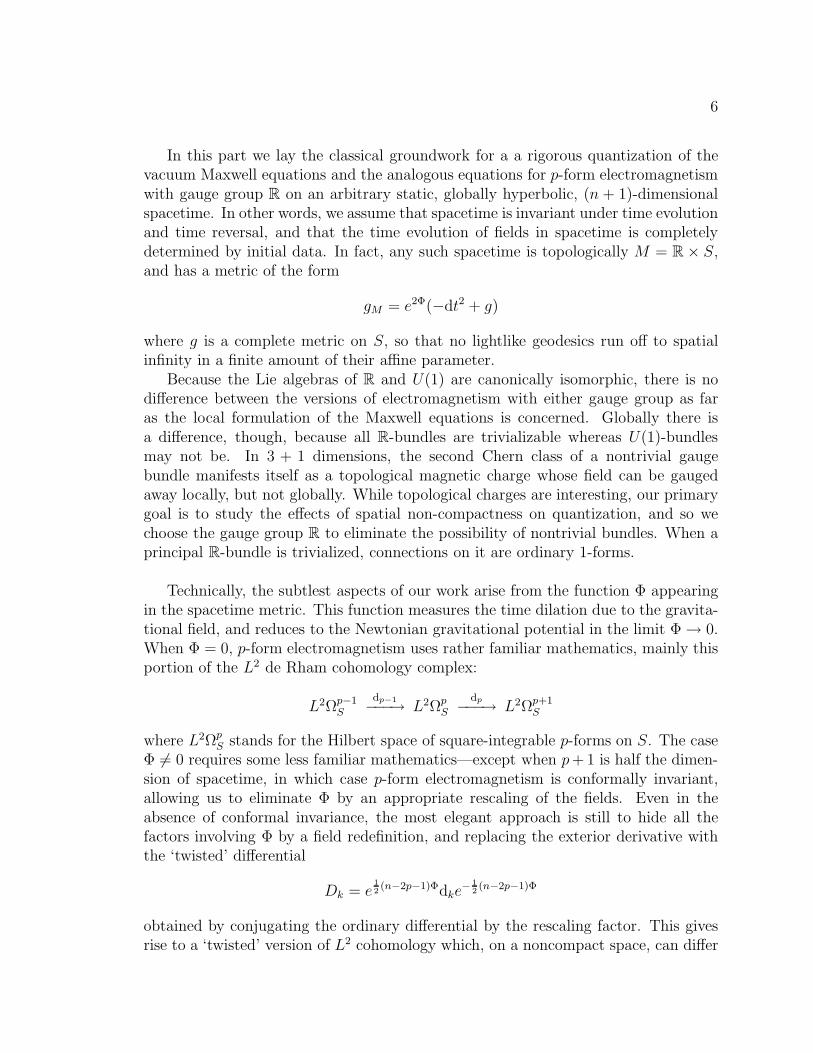
In this part we lay the classical groundwork for a a rigorous quantization of thevacuum Maxwell equations and the analogous equations for p-form electromagnetismwith gauge group R on an arbitrary static, globally hyperbolic, (n + 1)-dimensionalspacetime. In other words, we assume that spacetime is invariant under time evolutionand time reversal, and that the time evolution of fields in spacetime is completelydetermined by initial data. In fact, any such spacetime is topologically M = R × S,and has a metric of the form

gM = e2Φ(−dt2 + g)

where g is a complete metric on S, so that no lightlike geodesics run off to spatialinfinity in a finite amount of their affine parameter.

Because the Lie algebras of R and U(1) are canonically isomorphic, there is nodifference between the versions of electromagnetism with either gauge group as faras the local formulation of the Maxwell equations is concerned. Globally there isa difference, though, because all R-bundles are trivializable whereas U(1)-bundlesmay not be. In 3 + 1 dimensions, the second Chern class of a nontrivial gaugebundle manifests itself as a topological magnetic charge whose field can be gaugedaway locally, but not globally. While topological charges are interesting, our primarygoal is to study the effects of spatial non-compactness on quantization, and so wechoose the gauge group R to eliminate the possibility of nontrivial bundles. When aprincipal R-bundle is trivialized, connections on it are ordinary 1-forms.

Technically, the subtlest aspects of our work arise from the function Φ appearingin the spacetime metric. This function measures the time dilation due to the gravita-tional field, and reduces to the Newtonian gravitational potential in the limit Φ → 0.When Φ = 0, p-form electromagnetism uses rather familiar mathematics, mainly thisportion of the L2 de Rham cohomology complex:

L2Ωp−1S

dp−1−−−→ L2ΩpS

dp−−−→ L2Ωp+1S

where L2ΩpS stands for the Hilbert space of square-integrable p-forms on S. The case

Φ 6= 0 requires some less familiar mathematics—except when p+ 1 is half the dimen-sion of spacetime, in which case p-form electromagnetism is conformally invariant,allowing us to eliminate Φ by an appropriate rescaling of the fields. Even in theabsence of conformal invariance, the most elegant approach is still to hide all thefactors involving Φ by a field redefinition, and replacing the exterior derivative withthe ‘twisted’ differential

Dk = e12(n−2p−1)Φdke

− 12(n−2p−1)Φ

obtained by conjugating the ordinary differential by the rescaling factor. This givesrise to a ‘twisted’ version of L2 cohomology which, on a noncompact space, can differ

7

from the usual L2 cohomology which, in turn, can differ from the smooth de Rhamcohomology.

With this machinery in place we model the phase space of classical p-form electro-magnetism on (n+ 1)-dimensional spacetime as a real Hilbert space with continuousHamiltonian and symplectic stucture. In the process, we address the Aharonov–Bohmeffect in situations where the twisted L2 cohomology differs from the usual de Rhamcohomology, a subtle issue that is largely neglected in the literature.

Among the most rigorous published treatments of Maxwell’s equations on a fairlygeneric manifold stands that of Dimock [Dim92], which however is restricted to (3+1)-dimensional spacetimes with compact Cauchy surfaces. At the time of his writing,he said “nothing that follows is particularly new, but it seems that the various pieceshave not been put together”. A later paper reviewing the canonical and covariant for-mulations of the classical Maxwell theory on a generic globally hyperbolic spacetimeis the one by Corichi [Cor98], again “intended to fill an existing gap in the literature”.

Dimock constructs the classical phase space from gauge equivalence classes ofCauchy data and the symplectic structure obtained from the Noether current. Gaugefixing appears as a technical step used to show that Maxwell’s equations are strictlyhyperbolic, so that solutions are determined by their Cauchy data. Dimock uses“fundamental solutions” (essentially Green’s functions) to parameterize the phasespace, a technique that only works for linear field equations. Time evolution enters thepicture through symplectic transformations induced on phase space by changes in thechoice of Cauchy surface. In fact, Dimock makes “no choice of Hamiltonian or specialtime coordinate”, following the covariant canonical formalism of [CW87]. Dimockpoints out how the field strength does not provide a complete set of observableswhen the first homology class of the Cauchy surfaces is nontrivial. In Chapter 2 werelate this phenomenon to the Aharonov–Bohm effect and in Chapter 4 we presenta thorough overview of the situation in the non-compact case. Dimock assumes atrivial U(1)-bundle saying “presumably our results can be extended to non-trivialbundles for which A is only defined locally”, while we take the more drastic step ofassuming an R-bundle.

For the purposes of this Part, Dimock’s presentation of Maxwell’s equations doeshave a couple of important limitations. First, the restriction to compact Cauchysurfaces may be unphysical, and certainly excludes many cases of theoretical interest.We address the thorny analytic issues associated to allowing noncompact Cauchysurfaces in Chapter 2, albeit with the additional assumption that spacetime is static,which Dimock does not need. The topological implications of noncompactness arediscussed in Chapter 4. Dimock’s use of compact Cauchy surfaces allows his to bringHodge’s theorem to bear on the Cauchy data and, using the Kodaira decomposition,to show that the symplectic structure is non-degenerate. Although Hodge’s theoremdoes not hold on a noncompact space (see Chapter 4), we are nevertheless able toprove a form of Kodaira’s decomposition in Chapter 2.

Dimock also states without proof or reference that “for globally hyperbolic man-

8

ifolds, the usual classical linear field equations will have global solutions if they arewell-behaved locally. We quote the result for scalar fields”. We repaired this defect byreference to Chernoff’s work in Chapter 4. In the proof of existence of solutions withgiven Cauchy data Dimock states “The equation [above] has principal part gµν∂µ∂ν

and thus is strictly hyperbolic”; hyperbolicity easily follows from Chernoff’s work.Finally, the phase space constructed by Dimock does not have a topology other thanthat induced by imposing the continuity of the symplectic structure. Therefore, it isnot a real inner-product space like ours is.

While not assuming compact Cauchy surfaces, Corichi’s paper is “not very preciseabout functional-analytic issues” in the author’s own words. The covariant formula-tion is, like Dimock’s, based on the formalism of [CW87], and differs mostly in thenotation. The canonical formulation is written in a manifestly covariant way, in termsof the foliation generated by an arbitrary time coordinate function. Both formula-tions of classical electromagnetism are more general than ours, and the relationshipbetween Corichi’s covariant and canonical descriptions of phase space is equivalent toDimock’s treatment of Cauchy data in the covariant formalism.

The plan of this Part is as follows. We begin in Chapter 2 by setting up classicalelectromagnetism with gauge group R, leading up to Theorems 5 and 10, in which wemake the phase space for this theory into a real Hilbert space on which the classicalHamiltonian is a continuous nonnegative quadratic form. In Chapter 3 we generalizethis work to p-form electromagnatism in n+1 dimensions using the twisted de Rhamcomplex, leading up to the analogous Theorems 11 and 16. In Chapter 4 we surveywhat is known about L2 cohomology on noncompact spaces, and study a number ofexamples illustrating some of the associated subtleties.

9

Chapter 2

Classical vacuum electromagnetism

In this chapter we discuss the classical vacuum Maxwell equations on a (3 + 1)-dimensional static globally hyperbolic spacetime. In particular, we explain how theclassical phase space of electromagnetism splits into two parts, one containing the os-cillatory modes of the electromagnetic field and the other containing the ‘topological’modes responsible for the ‘Aharonov–Bohm’ effect.

The plan of this chapter is as follows: we begin in Section 2.1 by describingin detail our assumptions and notation concerning spacetime geometry, decomposespacetime in the form M ∼= R×S, and confront a number of analytical issues arisingfrom trying to define the exterior derivative on square-integrable differential forms.In Section 2.2 we give an overview of the stationary action formulation of classicalmechanics, and use it to derive the Maxwell equations, Noether current, Hamiltonianand symplectic structure, as well as kinematical, dynamical and physical phase spaces.Finally, in Section 2.3 we describe the splitting on the physical phase space of classicalvacuum electromagnetism into an sector consisting of oscillating modes, and a sectorconsisting of topological modes responsible for the Aharonov–Bohm effect.

After seeing that the spacetimes we are interested split in the form M ∼= R × S,where S is space, we define the exterior derivative d and coderivative d∗ so that theyact on square-integrable differential forms on space and satisfy

∫

S

g(α, dβ)vol =

∫

S

g(d∗α, β)vol (2.1)

whenever α and β are square-integrable differential forms of appropriate degrees.The key is to show that no ‘boundary terms at infinity’ appear in the integration byparts implicit in Equation (2.1). This can be used to show that the Laplacian onsquare-integrable differential forms is essentially self-adjoint and nonnegative, prop-erties necessary for rigorous quantization.

In the temporal gauge (vanishing electrostatic potential) the configuration spaceof classical electromagnetism on M consists of R-connections on S modulo gaugetransformations, and so is isomorphic to a space of 1-forms modulo square-integrable

10

exact 1-forms on S. In physics, such a 1-form is called a vector potential . We makethe configuration space into a real Hilbert space by defining it as

A =domd:L2Ω1

S → L2Ω2S

rand:L2Ω0S → L2Ω1

S

with its natural real inner product. That is, A consists of equivalence classes ofsquare-integrable 1-forms with square-integrable exterior derivatives, modulo exact1-forms. This space is naturally a real Hilbert space.

The canonical conjugate of the vector potential [A] is a divergenceless 1-form E,called the electric field . The space of electric fields

E = kerd∗:L2Ω1S → L2Ω0

S

is also naturally a real Hilbert space. The phase space of classical electromagnetismis, then, the real Hilbert space

P = A ⊕ E.

The spaces A and E are dual to each other by

([A], E) =

∫

S

g(A,E)vol,

which is independent of the representative A chosen for [A] because E is divergence-less. The symplectic structure on P is constructed from this duality pairing by anti-symmetrization:

ω([A] ⊕ E, [A′] ⊕E ′) =

∫

S

[g(A,E ′) − g(A′, E)]vol.

Because of global hyperbolicity, any point X = [A]⊕E of the physical phase spacedetermines a unique solution of Maxwell’s equations on all of M . Time evolution isgiven by a continuous one-parameter group of continuous symplectic transforma-tions T (t):P → P. Unlike the symplectic structure and the Hamiltonian, the naturalHilbert space norm on P is not preserved by this time evolution.

As a result of gauge-fixing, when restricted to the phase space the Laplacian on 1-forms is ∆ = d∗d. The assumption that spacetime is static then implies that timeevolution commutes with ∆, and so the phase space admits the decomposition

P = Po ⊕Pf

where Pf is the kernel of ∆ in P and consists of generalized Aharonov–Bohm modes.From the point of view of dynamics, the direct summand Po consists of ‘oscillatingmodes’ and Pf of ‘free modes’. Specifically, on Po the Hamiltonian is a positive-definite quadratic form, and so that ‘sector’ of the electromagnetic field has the

11

dynamics of an infinite-dimensional harmonic oscillator. The free sector Pf has dy-namics analogous to those of a free particle. For the free sector one can successfullyapply the algebraic approach to quantization of Chapter 5, but the existence of aHilbert-space representation on which time evolution is unitarily implementable isnot guaranteed unless Pf is finite-dimensional. As we shall see in Chapter 4, thatmay not be the case on a noncompact space even if it is topologically trivial.

12

2.1 Geometric setting

In this section we describe the mathematical framework for our study of clas-sical electromagnetism, and explain the mathematical reasons why various physicalrestrictions are imposed on the class of spacetimes under consideration.

2.1.1 Static globally hyperbolic spacetimes

Let us begin by recalling the precise definition of a static, globally hyperbolicspacetimes. In physical terms, a spacetime is stationary if it is invariant under timetranslations and static if, in addition, it is invariant under time reversal. Our firstdefinition casts these intuitive concepts in the language of (pseudo-)Riemannian ge-ometry.

Definition 1 (stationary and static spacetimes). A Lorentzian manifold withouttimelike loops (also called a spacetime) is stationary if, and only if, it admits a one-parameter group of isometries with smooth, timelike orbits. A stationary spacetime isstatic if, in addition, it is foliated by a family of spacelike hypersurfaces everywhereorthogonal to the orbits of the isometries.

Note. Spacetimes with closed timelike loops lead to a breakdown of the ordinaryinitial-value formulation of dynamics, and so must be excluded from our analysis.Diffeomorphism with smooth, timelike orbits are generated by an everywhere time-like vector field. A vector field generating isometries is called a Killing vector field ,and the isometries generated by a timelike Killing field are called time translations.A stationary spacetime M is diffeomorphic to R × S for some smooth manifold Srepresenting ‘space’; if, in addition, M is static, it admits a metric of the form

gM = −e2Φdt2 + gS,

where Φ is a time-independent function on S, and gS is a time-independent Rie-mannian metric on S. A stationary spacetime would require cross-terms of theform eΦ(dt ⊗ α + α ⊗ dt) in the metric, α being a nonzero time-independent 1-formon S. For proofs of these statements see, for instance, [Wal84].

The concept of global hyperbolicity is more subtle, but it is related to the simpleidea of causality: that points of spacetime are partially ordered by the relation ‘beingto the future of’. The name ‘global hyperbolicity’ originally referred to a property ofsystems of partial differential equations on Euclidean space. By reinterpreting thoseequations as coordinate representations of equations adapted to a curved Lorentzianmanifold, the hyperbolicity of the system became a geometric property of the space-time itself (see [Ger70] and references therein). As we shall see, global hyperbolicityof the spacetime implies that the evolution equations of massless fields are globallyhyperbolic systems of partial differential equations.

13

Hyperbolic systems of partial differential equations have a finite propagation veloc-ity, meaning that compactly-supported initial data evolve into compactly-supportedsolutions after a finite time. Under the reinterpretation of hyperbolic systems as prop-agation equations on Lorentzian manifolds, the finite propagation velocity means thatsolutions with compactly-supported initial data are completely contained in the lightcones of the support of their initial data. This is one of the manifestations of causality.

The following definition formalizes the geometric ideas of causality and globalhyperbolicity.

Definition 2 (globally hyperbolic spacetime). A piecewise-smooth curve in aspacetime M is causal if its tangent vector is everywhere timelike. A set is achronalif there are no causal curves between any two of its points. The domain of dependenceof a set consists of all points p ∈M such that every inextensible causal curve through pintersects the set. A Cauchy surface in a spacetime M is a closed achronal set whosedomain of dependence is all of M . A spacetime is globally hyperbolic if, and only if,it admits a Cauchy surface.

Note. The domain of dependence is also called the Cauchy development . Both names,‘domain of dependence’ and ‘Cauchy development’, betray their origin in the theory ofpartial differential equations, as does the term ‘Cauchy surface’. A Cauchy surface in aspacetime M is an achronal set intersecting every inextensible causal curve in M . It isnot hard to see that closed timelike curves cannot intersect an achronal hypersurface,and so spacetimes with closed timelike curves cannot be globally hyperbolic. For astatic spacetime with metric

gM = e2Φ(−dt2 + g), (2.2)

global hyperbolicity is equivalent to completeness of the metric g = e−2ΦgS. Thismetric g is sometimes called optical metric (see, for instance, [TdCMP99, KSA98,Sta84, Ehl66]) because light rays follow geodesics of this metric. More precisely,the geodesics of g parameterized by arc length lift to affinely parameterized lightlikegeodesics of −dt2 + g, with the time t corresponding to the arc-length parameter ongeodesics of g. Hence, the propagation of light in the geometric optics approximationis determined by g alone. We will consistently use the optical metric g on S ratherthan gS.

2.1.2 Spacetime geometry and topology

We model spacetime as a static, globally hyperbolic, (3+1)-dimensional Lorentzianmanifold. That is, spacetime will be represented by a smooth (3 + 1)-dimensionalmanifold M diffeomorphic to R × S and admitting a Lorentzian metric of the formgiven in Equation (2.2).

14

For convenience, we also assume S is oriented. In that case, the metric g de-termines a volume form vol on S. Similarly, the spacetime M acquires a volumeform volM from the metric gM . The canonical volume forms are related by

volM = e4Φvol ∧ dt. (2.3)

If S were nonorientable, we could still carry through our whole discussion with minormodifications, the most important of which being that vol and volM would have tobe treated as densities.

We religiously follow the convention of writing all differential forms on spacetimewith a subscript ‘M ’. We also write the so-called temporal part with a subscript ‘0’,and the spatial part with no subscript. We decompose k-forms on M into spatial andtemporal parts thus:

αM = dt ∧ α0 + α, (2.4)

where α0 is a (k − 1)-form and α is a k-form on S, both t-dependent.The exterior derivative operators on spacetime dM :C∞

0 ΩkM → C∞

0 Ωk+1M and on

space d:C∞0 Ωk

S → C∞0 Ωk+1

S , where C∞0 Ωk

S denotes smooth, compactly supported k-forms on S, are related by dM = dt ∧ ∂t + d; in other words,

dMαM = dt ∧ (∂tα− dα0) + dα. (2.5)

for all compactly-supported smooth k-forms αM ∈ C∞0 Ωk

M .We use g and gM to denote the respective induced metrics on k-forms, satisfying

gM(αM , βM) = e−2kΦ[g(α, β)− g(α0, β0)], (2.6)

and define the positive-definite bilinear forms

(αM , βM)M =

∫

M

gM(αM , βM)volM and (α, β) =

∫

S

g(α, β)vol (2.7)

on C∞0 Ωk

M and C∞0 Ωk

S , which are related by

(αM , βM)M =

∫

R

e(4−2k)Φ[(α, β) − (α0, β0)]dt. (2.8)

We denote by δ the formal adjoint of d with respect to the bilinear form ( , ).This means that the operator δ:C∞

0 Ωk+1S → C∞

0 ΩkS is defined by

(α, dβ) = (δα, β) for all α ∈ C∞0 Ωk+1

S and β ∈ C∞0 Ωk

S, (2.9)

The compact support in Equations (2.5) and (2.9) has the function of avoiding bound-ary terms on the implicit integration by parts involved in the definition of δ.

15

2.1.3 Issues of analysis on noncompact spaces

A restatement of Equation (2.9) is the existence of operators

C∞0 Ωk

S

d //C∞

0 Ωk+1S

δoo (2.10)

which are formal adjoints of each other. Our goal is to extend these to densely definedoperators between L2Ωk and L2Ωk+1 which are adjoint to each other in the strict senseof operator theory, where L2Ωk denotes the space of square-integrable k-forms on S.It turns out that this can be done precisely because g is a complete metric on S,which we have seen is equivalent to global hyperbolicity of spacetime.

There are both physical and mathematical reasons for wanting to do this. Mathe-matically, a mutually adjoint pair of unbounded operators between two Hilbert spacesare much better behaved than formally-adjoint operators between spaces of smoothdiferential forms, although the latter have more intuitive geometric appeal. From aphysical point of view, we do not wish to restrict ourselves to compactly-supportedfields in a noncompact space, but on the other hand we need the fields to be squareintegrable in order for the Hamiltonian and symplectic structure on phase space tobe finite at all times. These sorts of physical considerations demand that we treat dand δ as unbounded operators between Hilbert spaces of square-integrable differentialforms. To prove that time evolution maps the classical phase space to itself, we willalso need to extend δd to an unbounded self-adjoint operator on square-integrable1-forms. Finally, once we insist on interpreting d as an operator between spaces ofsquare-integrable forms, the electromagnetic gauge transformations will need to havesquare-integrable generators.

All this requires a short detour into functional analysis, which is contained in thissubsection. While the facts we need are well-known to the experts, they may beunfamiliar to some readers, so we review them in a fair amount of detail. We omitmost of the proofs, many of which can be found in Reed and Simon’s textbook [RS80].The reader who is more interested in the physical use of these operators can skip toSection 2.2, with the observation that from then on the operator δ is denoted d∗, asin

L2ΩkS

d //L2Ωk+1

Sd∗

oo , (2.11)

in order to free the symbol δ for use in variational calculus. Making sense of Equa-tion (2.11) is the main purpose of this subsection.

In going from Equation (2.10) to Equation (2.11), the first thing we need to dois establish that the operators d:C∞

0 ΩkS → C∞

0 Ωk+1S and δ:C∞

0 Ωk+1S → C∞

0 ΩkS ap-

pearing in Equations (2.9) and (2.10) can be interpreted as densely-defined operatorsbetween L2Ωk

S and L2Ωk+1S . This follows from Lemma 1.

Lemma 1. The completion of C∞0 Ωk

S with respect to the inner product ( , ) is L2ΩkS.

16

Proof. We can reduce this to the well-known case where S = Rn using a partition-of-unity argument.

The domain of the operator d is the dense subspace

dom d = C∞0 Ωk

S ⊆ L2ΩkS.

We then define the adjoint d∗ in the usual way, as follows. First, the domain of d∗

consists of all α ∈ L2Ωk+1S for which there exists a γ ∈ L2Ωk

S such that

(α, dβ) = (γ, β)

for all β ∈ C∞0 Ωk

S . If such a γ exists it is unique because C∞0 Ωk

S is dense in L2ΩkS,

and we then define d∗α to equal this γ, so that

(α, dβ) = (d∗α, β) ∀β ∈ C∞0 Ωk

S . (2.12)

as desired. Note that, because β is required to be of compact support, α is notrequired to have compact support.

Similarly, the dense domain of δ is C∞0 Ωk+1

S , the domain of δ∗ is not restricted tocompactly-supported forms, and δ∗β can be defined by

(α, δ∗β) = (δα, β) ∀α ∈ C∞0 Ωk+1

S .

We can also define operators d and δ, the respective closures of d and δ. For dthis goes as follows. We define the graph of d to be the linear subspace

Gr(d) = α⊕ dα | α ∈ C∞0 Ωk

S ⊆ L2ΩkS ⊕ L2Ωk+1

S

where the latter space is a Hilbert space in an obvious way. This subspace is typicallynot closed, and we say that d is closable if the closure of Gr(d) is the graph of anoperator, which we then denote d. In other words,

α ∈ domd ⇔ α = limn→∞

αn and dαn → dα for some αn ∈ C∞0 Ωk

S . (2.13)

We define the closure δ in essentially the same way.Because of Equation (2.9) both d∗ and δ∗ are densely defined, so the following

lemma applies.

Lemma 2. A densely defined operator T is closable if, and only if, T ∗ is denselydefined. In that case, T = T ∗∗.

Observe that T ∗ is automatically closed and T∗

= T ∗. As a result, d = d∗∗ andδ = δ∗∗. We have d ⊆ d ⊆ δ∗ and δ ⊆ δ ⊆ d∗.

Proof. See Reed and Simon’s textbook [RS80, Theorem VIII.1].

17

We have argued that

dom d ⊆ dom δ∗ and dom δ ⊆ dom d∗,

but d and δ will be mutual adjoints only if these are actually equalities. Having thembe mutual adjoints is highly desirable, as otherwise there are at least two possibleself-adjoint extensions of the operator δd, namely d∗d and δδ∗. This means we needto understand how the equations dom d = dom δ∗ and dom δ = dom d∗ could fail tohold.

The answer has to do with boundary values. Suppose that S is a relatively compactopen subset of some larger Riemannian manifold X, and its boundary ∂S is a smoothsubmanifold of X. In this case the desired equalities never hold, and there is a well-developed theory of boundary values which explains why [Eva98]. In brief, if α, β arecompactly supported smooth forms on S, integration by parts gives

(dα, β) = (α, δβ) for all α ∈ C∞0 Ωk

S and β ∈ C∞0 Ωk+1

S .

From this, an approximation argument gives

(dα, β) = (α, δβ) if α ∈ dom d and β ∈ dom δ.

On the other hand, if α, β are merely smooth forms on S that extend smoothly to X,integration by parts gives

(dα, β) − (α, δβ) = (α, β)∂S, for all α ∈ C∞ΩkS and β ∈ C∞Ωk+1

S (2.14)

and from this, again by an approximation argument, one can show

(δ∗α, β) = (α, d∗β) + (α, β)∂S if α ∈ dom δ∗ and β ∈ dom d∗.

Thus we cannot have dom d = dom δ∗ and dom δ = dom d∗ in this case: the nonzeroboundary term (α, β)∂S gets in the way.

The same sort of problem can occur even when S is not a relatively compact opensubset of some larger Riemannian manifold. However, in this more general situa-tion the concept of ‘boundary value’ needs to be reinterpreted as ‘value at spacelikeinfinity’. In fact, Equation (2.14) can be used to define the notion of boundary atinfinity of S. The domain of d can be understood as the space of square-integrabledifferential forms with square-integrable exterior derivatives and vanishing ‘values atinfinity’, while the domain of δ∗ consists of square-integrable differential forms withsquare-integrable exterior derivatives and no restriction on values at infinity. Thus,the desired equation d = δ∗ fails to hold if an element of dom δ∗ can fail to ‘vanishat infinity’. Similar remarks apply to the equation δ = d∗. Simply put, the problemsarise when there are boundary terms at infinity when we integrate by parts.

Luckily, the folowing result of Gaffney implies that these problems never happenwhen g is a complete Riemannian metric on S.

18

Proposition 3 (Gaffney). If S is a complete oriented Riemannian manifold, then

(δ∗α, β) = (α, d∗β)

whenever α ∈ dom δ∗ and β ∈ dom d∗.

Gaffney calls manifolds where the conclusion of Proposition 3 holds “manifoldswith negligible boundary”.

Proof. This can be found in Gaffney’s paper [Gaf54]; we will also give a proof of amore general result in Corollary 15, based on work of Chernoff [Che73].

Corollary 4. If S is a complete oriented Riemannian manifold, then

d = δ∗ and δ = d∗.

This means that d and δ have mutually adjoint closures

L2Ωkd //L2Ωk+1

δ

oo .

As we pointed out above, this implies that the operators δd and dδ have uniqueself-adjoint closures.

Proof. We will prove that d = δ∗, as the other equality then follows by lemma 2.We already know that d ⊆ δ∗, so we need only show that δ∗ ⊆ d. To this end, letα ∈ dom δ∗ and β ∈ dom d∗. By Lemma 1, α ∈ dom δ∗ is the L2 limit of a sequence αn

of compactly-supported differential forms. Gaffney’s Proposition 3 allows us to write

(δ∗α | β) = (α | d∗β) = limn→∞

(αn | d∗β)

By the definition of d∗ in Equation (2.12),

(δ∗α | β) = limn→∞

(αn | d∗β) = limn→∞

(dαn | β).

Since this holds for arbitrary β in the dense domain of d∗, not only αn → α but alsodαn → δ∗α, and so α ∈ domd and dα = δ∗α by the definition of d in Equation (2.13).

As we shall see, the uniqueness of the self-adjoint closure of δd (in other words, theessential self-adjointness of δd) is necessary to make sense of the Fock quantizationof the electromagnetic field. By Gaffney’s result, the essential self-adjointness of δdfollows from completeness of S which, as we have pointed out, is equivalent to theglobal hyperbolicity of the original static spacetime M . Intuitively, if a spacetimeis globally hyperbolic there is no information coming from or lost to infinity, so no

19

boundary conditions are necessary to uniquely determine time evolution of square-integrable differential forms and, in fact, space has ‘negligible boundary’ in the senseof Gaffney. This, in retrospect, is the justification for the assumption that spacetime isglobally hyperbolic although, strictly speaking, this is a sufficient but not a necessarycondition for S to have negligible boundary.

Because our assumption of global hyperbolicity implies that d = δ∗ and δ = d∗

there is no ambiguity in the closing of the operators d and δ, and from this point on weshall assume that d and δ have been closed unless otherwise stated. We will slightlyabuse notation by writing d to denote the closed version of the exterior derivative. Asnoted before, its adjoint will be denoted d∗ so as to preserve δ for use in variationalcalculus.

Sometimes, as shorthand or in order to avoid confusion between exterior derivativeoperators acting on different spaces, an additional bit of notation will be necessary;namely, we will denote by dk the operator d:L2Ωk

S → L2Ωk+1, so that d∗k will stand

for d∗:L2Ωk+1S → L2Ωk

S.

2.2 Maxwell’s theory

In the rest of this section we derive the Maxwell equations by applying Hamilton’sprinciple of stationary action, and define the phase space of the theory as the collectionof gauge equivalence classes of solutions of the equations of motion. The phase spaceis constructed in three steps (see, for instance, [Rov02a, Rov02b]): a kinematicalphase space on which the Hamilton least action principle can be formulated, butnot supporting a Hamiltonian or symplectic structure; a dynamical phase space ofsolitions of the equations of motion on which a conserved Hamiltonian and Noethercurrent are defined, but without a symplectic structure; and a physical phase spacewith no remaining gauge freedom, which is a symplectic space.

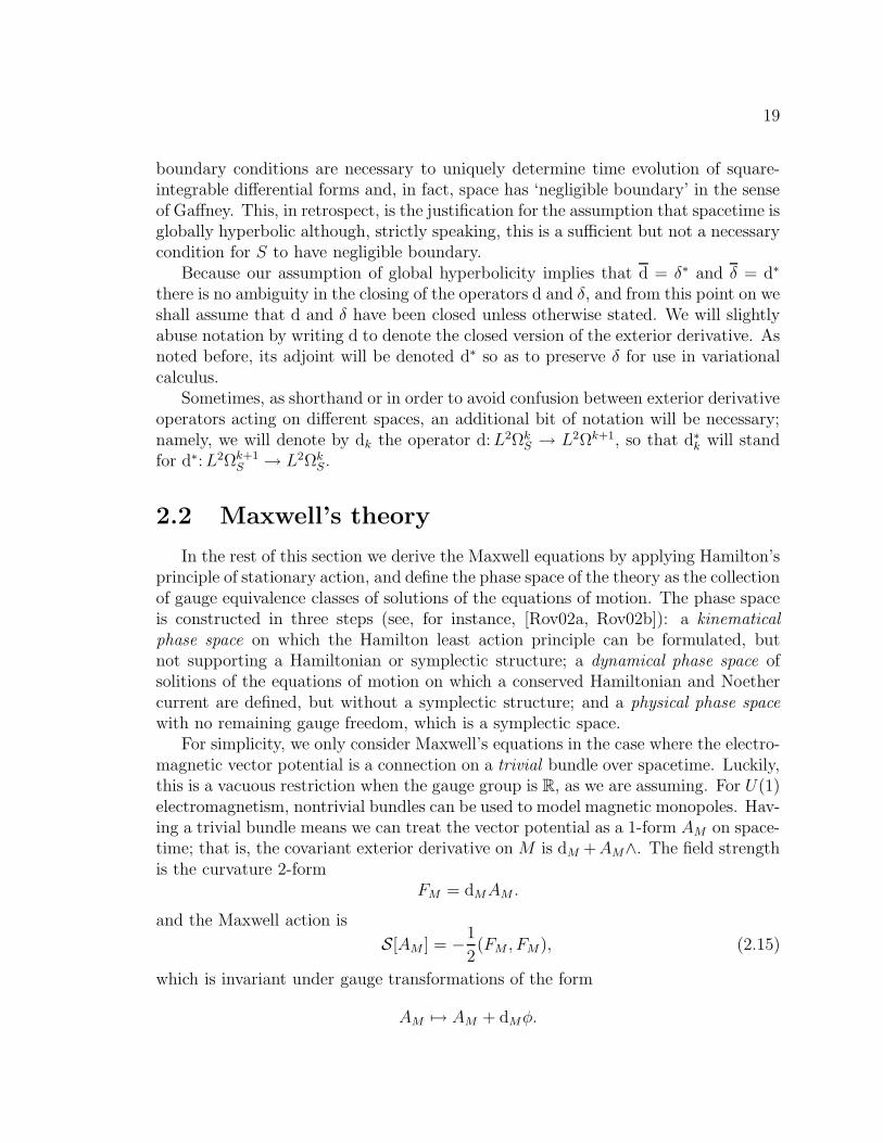
For simplicity, we only consider Maxwell’s equations in the case where the electro-magnetic vector potential is a connection on a trivial bundle over spacetime. Luckily,this is a vacuous restriction when the gauge group is R, as we are assuming. For U(1)electromagnetism, nontrivial bundles can be used to model magnetic monopoles. Hav-ing a trivial bundle means we can treat the vector potential as a 1-form AM on space-time; that is, the covariant exterior derivative on M is dM +AM∧. The field strengthis the curvature 2-form

FM = dMAM .

and the Maxwell action is

S[AM ] = −1

2(FM , FM), (2.15)

which is invariant under gauge transformations of the form

AM 7→ AM + dMφ.

20

The equations of motion follow from applying the Hamilton principle of stationaryaction to Equation (2.15).

To obtain a Hamiltonian formulation of the equations of motion one needs to usean explicit foliation of spacetime into a family of Cauchy surfaces related by a timetranslation symmetry. We can do this because we have assumed that spacetime isglobally hyperbolic and static. We use Equation (2.4) to split AM and FM into spatialand temporal parts:

AM = dt ∧A0 + A and FM = dt ∧ F0 + F,

whose physical interpretation is that F0 is the electic field and F the magnetic field,as we shall see below. By Equation (2.5)

F0 = ∂tA− dA0 and F = dA.

Gauge transformations leave FM unchanged, but their effect on A0 and A is

A 7→ A + dφ and A0 7→ A0 + ∂tφ. (2.16)

Using Equation (2.8), Equation (2.15) can be rewritten as

S[A,A0] =1

2

∫

R

[(∂tA− dA0, ∂tA− dA0) − (dA, dA)]dt. (2.17)

Note that a factor of e−4Φ in the metric on 2-forms from Equation (2.6) has cancelledthe factor of e4Φ in the volume form on spacetime from Equation (2.3). This makesthe 3 + 1-dimensional case of Maxwell’s theory special, and it is intimately relatedto the fact that Maxwell’s equations are conformally invariant in this dimension.Conformal invariance is another reason why the decomposition gM = e2Φ(−dt2 +g) ispreferable to gM = −e2Φdt2 + gS, at least in this case. The action of Equation (2.17)is the time-integral of the Lagrangian

L[A,A0] =1

2[(A− dA0, A− dA0) − (dA, dA)], (2.18)

where A = ∂tA.Because of energy conservation, the integral of Equation (2.17) is likely to diverge

unless it is restricted to a finite interval of t. This restiction is, in any case, necessaryto use the action principle to study time evolution between two given instants of time.In addition to evaluating the action integral over a finite interval of time, sufficientconditions for Equations (2.16)–(2.18) to make sense include that

φ(t), A0(t) ∈ domd:L2Ω0S → L2Ω1

S and A(t) ∈ domd:L2Ω1S → L2Ω2

S,

for almost, with t with all the L2 norms being square-integrable over any compactinterval of t; and that their respective time derivatives are in the same spaces. This

21

S

MR

Figure 2.1: Schematic representation of spacetime, space and the domain of integra-tion for the action functional

imposes nontrivial smoothness and decay restrictions on the electromagnetic poten-tials A0, A, and also on the allowed generators φ of gauge transformations. In the casewhen space is compact, any smooth gauge generator will automatically be boundedand square-integrable, but in the noncompact case we are forced to exclude somegauge transformations which are too large at infinity but would otherwise naıvely beallowed. This restriction on the gauge generators cannot manifest itself in physicaleffects on any bounded region of spacetime.

2.2.1 Overview of covariant mechanics

Hamilton’s principle states that physically allowed field configurations X in aregion R of a spacetime M are critical points (not necessarily minima) of an actionfunctional SR[X]. We assume that the action is local, that is, that SR[X] is theintegral over the spacetime region R of a Lagrangian density L[X] which, at eachpoint of spacetime, depends only on X and a finite number of its derivatives (usuallyjust the first) at that point. The action functional is often calculated by evaluatingthe integral in Equation (2.17) over a bounded region of spacetime, and almost alwaysover a finite interval of time. In fact the action calculated over all of time may beinfinite, and the variation of the action might also be ill-defined unless restricted to becompactly supported in time, which amounts to evaluating the action integral overa finite interval of time in the first place. Hamilton’s principle is formulated on akinematical phase space XR large enough to contain all plausible field configurationsand small enough that SR[X] =

∫RL[X] is well-defined.

The stationary action principle implies the vanishing of the first variation of theaction on any region R:

0 = δSR[X] =

∫

R

δL[X] = −∮

∂R

θ[X] +

∫

R

E[X].

It has been shown [Zuc87, CW87] that it is possible and advantageous to choose Xto be an infinite-dimensional manifold (possibly even a vector space) and interpretthe variational derivative δ as an exterior derivative on X. The Lagrangian density Lis then an (n + 1)-form on X ×M proportional to volM . The condition that L bea local Lagrangian means that, at any point p ∈ M , L depends on X only through

22

the values of X and finitely many ot its derivatives at p. The exterior derivativeon X ×M is δ + dM , which implies the anticommutation relation δdM + dMδ = 0.The quantity E is an (n + 2)-form on X ×M which is a 1-form with respect to Xand proportional to the (n + 1)-form volM ; similarly, θ is an (n + 1)-form which isa 1-form with respect to X and an n-form with respect to M . Tangent vectors to Xare variations of field configurations. We denote a typical such tangent vector by ∂X .

If δSR[X] is evaluated at a stationary field configuration X, on variations ∂X

vanishing on the boundary ∂R, the stationary action condition implies the Euler–Lagrange equations of motion E[X](∂X) = 0. We define the dynamical phase spaceassociated to the region R as the variety

DR = X ∈ X:E[X](∂X) = 0 on R if ∂X = 0 on ∂R.

The so-called Noether current θ[X] is defined only up to an exterior derivative,and can be interpreted as a generator of conserved quantities associated to continuoussymmetries of solutions to the Euler–Lagrange equations of motion. To see this,consider a tangent vector to DR, which is a variation of solutions to the Euler–Lagrange equations of motion. Because the Euler-Lagrange equations are satisfiedthroughout, we have ∮

∂M

θ[X](∂X) = 0.

Suppose now that R ∼= [0, 1] × T . Then,∫

T0

θ[X](∂X) −∫

T1

θ[X](∂X) =

∫

[0,1]×∂T

θ[X](∂X),

where the right-hand side represents the time integral of the flux of the conservedquantity through ∂T . In the case where R is a globally hyperbolic region with Cauchysurface T , the latter has negligible boundary in the sense of Gaffney, and

∫

T0

θ[X](∂X) =

∫

T1

θ[X](∂X),

so∫

Tθ[X](∂X) is a conserved quantity of the motion. For instance, in the case

where M ∼= R × S is static and R = [t0, t1] × S, the variation ∂X might representthe generator of a one-parameter group of isometries of S (a translation or rotation)on the field configuration X, and the associated conserved quantity would be thecorresponding momentum (linear or angular) of X. If ∂X represented the action ofan internal symmetry of the field variables at each point (a gauge transformation), theconserved quantity would be the conserved charge associated to the gauge symmetry.

The variational derivative of the Noether current is a skew-symmetric 2-formon DR,

ωT [X] =

∫

T

δθ[X].

23

?????????????

????

????

????

?

T

R

Figure 2.2: Schematic representation of a globally hyperbolic region foliated by afamily of Cauchy surfaces.

Given two variations of solutions,

ωT [X](∂X , ∂′X)

is a conserved quantity of the solution X. It is possible that ωT [X] is degenerate,admitting variations of solutions ∂X such that

ωT [X](∂X ,−) = 0.

Each such degenerate direction ∂X generates a gauge transformation of the dynamicalphase space. The space of gauge orbits of DR is the physical phase space PR. As wehave pointed out, it is in general not a manifold, but an ‘infinite-dimensional varietywith singularities’. By construction, ωS would project to a non-degenerate symplecticstructure on PR.

A more cogent approach to the physical phase space PR would be as follows.Let N denote the space of degenerate directions of ωT . The smooth functions fon DR such that ∂Xf = 0 whenever ∂X ∈ N constitute a subalgebra of C∞(DR),the so-called gauge-invariant observables on DR. The spectrum of homomorphismsof this algebra would be PR, and we can map the algebra of gauge-invariant observ-ables homeomorphically to C∞(PR). Whether or not PR turns out to be a manifoldthat can support a symplectic structure, the algebra of gauge-invariant supports thecanonical Poisson structure

f, g = ωT (∂f +N, ∂g +N) for all f ∈ C∞(PR),

where ∂f is a tangent vector to DR such that ωT (∂f , ∂Y ) = δf(∂Y ) for all tangentvectors to DR. Conveniently, ∂f is defined precisely up to addition of elements of N ,so one can associate a unique equivalence class in TDR/N to it, namely ∂f + N .Since ωT is, in fact, non-degenerate on DR, the algebra of gauge-invariant observablesis a Poisson algebra, whose spectrum is the physical phase space.

This construction simplifies considerably when the action functional is quadratic,as in that case the equations of motion and the Noether current are linear, and allthe spaces involved are vector spaces. In addition, in a stationary, globally hyperbolic

24

spacetime M there is a preferred foliation M ≃ R × S by Cauchy surfaces isometricto S. When there is a single timelike Killing field, there is a canonical identificationof the different Cauchy surfaces, and time evolution can be represented as a trans-formation of the field configuration on a single Cauchy surface. It is then possible todefine a Hamiltonian function.

In the next few sections we construct the phase space of electromagnetism usingthis method. First, the kinematical phase space is a space X of field configurations onwhich the Maxwell action can be defined, or on which the Maxwell equations can bewritten. The precise definition of the kinematical phase space is somewhat arbitrary,as long as it is large enough to contain all the actual solutions of the equations ofmotion. In the next section we shall see three acceptable formulations of the leastaction principle on different kinematical phase spaces before settling on one of them.

Next, setting the first variation of the action to zero yields the Maxwell equationsof motion, whose space of solutions if the dynamical phase space D and is a linearsubspace of the kinematical phase space (in more general cases, D is just a subvarietyof X). The dynamical phase space supports the Hamiltonian and Noether currentof the system, which can be used to obtain conserved quantities of the system anda pre-symplectic structure on D. The null directions of the pre-symplectic structureare seen to correspond to gauge transformations.

Finally, the set P of gauge orbits on D is the physical phase space or, simply, thephase space. When there is no gauge freedom, the dynamical phase space coincideswith the physical phase space. After this reduction from D to P, the pre-symplecticstructure on D becomes a non-degenerate symplectic structure on P.

2.2.2 Kinematical phase space

In this section we consider three possible action principles for electromagnetismon slightly different kinematical phase spaces. The first is the Lagrangian formula-tion of Equations (2.17–2.18). The second formulation is the associated Hamiltonianformulation, with the electrostatic potential A0 acting as a Lagrange multiplier en-forcing the Gauss law as a constraint. Since the latter is linear, it is possible andeven convenient to impose the Gauss law at the kinematical level without a Lagrangemultiplier. This is the third formulation.

All three kinematical phase spaces are equivalent in that the action principlesdefined on them lead to the same space of solutions of the equations of motion.However, the three kinematical phase spaces are not isomorphic to each other. Thefirst requires that A0 be in the domain of d, and that E = ∂tA − dA0 be square-integrable. The second alternative allows A0 to be just square integrable, but E mustnow be in the domain of d∗. The third formulation does without A0 altogether, but Emust be in the kernel of d∗.

25

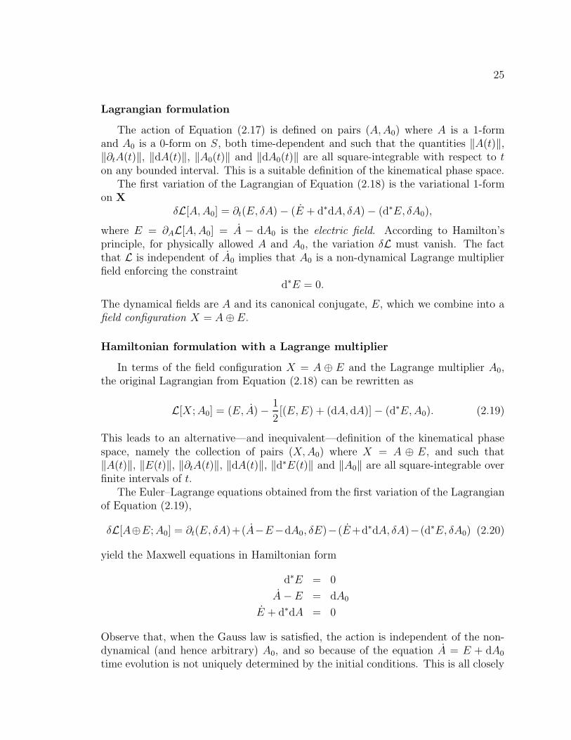
Lagrangian formulation

The action of Equation (2.17) is defined on pairs (A,A0) where A is a 1-formand A0 is a 0-form on S, both time-dependent and such that the quantities ‖A(t)‖,‖∂tA(t)‖, ‖dA(t)‖, ‖A0(t)‖ and ‖dA0(t)‖ are all square-integrable with respect to ton any bounded interval. This is a suitable definition of the kinematical phase space.

The first variation of the Lagrangian of Equation (2.18) is the variational 1-formon X

δL[A,A0] = ∂t(E, δA) − (E + d∗dA, δA) − (d∗E, δA0),

where E = ∂AL[A,A0] = A − dA0 is the electric field. According to Hamilton’sprinciple, for physically allowed A and A0, the variation δL must vanish. The factthat L is independent of A0 implies that A0 is a non-dynamical Lagrange multiplierfield enforcing the constraint

d∗E = 0.

The dynamical fields are A and its canonical conjugate, E, which we combine into afield configuration X = A⊕E.

Hamiltonian formulation with a Lagrange multiplier

In terms of the field configuration X = A ⊕ E and the Lagrange multiplier A0,the original Lagrangian from Equation (2.18) can be rewritten as

L[X;A0] = (E, A) − 1

2[(E,E) + (dA, dA)] − (d∗E,A0). (2.19)

This leads to an alternative—and inequivalent—definition of the kinematical phasespace, namely the collection of pairs (X,A0) where X = A ⊕ E, and such that‖A(t)‖, ‖E(t)‖, ‖∂tA(t)‖, ‖dA(t)‖, ‖d∗E(t)‖ and ‖A0‖ are all square-integrable overfinite intervals of t.

The Euler–Lagrange equations obtained from the first variation of the Lagrangianof Equation (2.19),

δL[A⊕E;A0] = ∂t(E, δA)+(A−E−dA0, δE)−(E+d∗dA, δA)−(d∗E, δA0) (2.20)

yield the Maxwell equations in Hamiltonian form

d∗E = 0

A−E = dA0

E + d∗dA = 0

Observe that, when the Gauss law is satisfied, the action is independent of the non-dynamical (and hence arbitrary) A0, and so because of the equation A = E + dA0

time evolution is not uniquely determined by the initial conditions. This is all closely

26

related to the existence of time-dependent gauge transformations, which by Equa-tion (2.16) result in a change of the Lagrange multiplier field A0. We can use thisgauge freedom to eliminate the Lagrange multiplier A0, that is, we perform a time-dependent gauge transformation to make A0 = 0. This is the so-called ‘temporalgauge’. Then, the Maxwell equations take the form

d∗E = 0 (Gauss law constraint) (2.21)

A− E = 0 (Faraday–Lenz law) (2.22)

E + d∗dA = 0 (Ampere–Maxwell law) (2.23)

on the kinematical phase space.

Hamiltonian formulation without Lagrange multipliers

The partial gauge-fixing of the previous case can be carried out at the level ofthe action, leading to a third possible definition of the kinematical phase space X,consisting of pairs X = A⊕ E such that ‖A(t)‖, ‖∂tA(t)‖, ‖dA(t)‖, and ‖E(t)‖ aresquare-integrable on finite intervals of t, and that d∗E(t) = 0 for almost all t.

We choose this as our preferred kinematical phase space. This means that, forus, X consists of pairs X = A⊕ E such that

A(t) ⊕ E(t) ∈ domd:L2Ω1S → L2Ω2

S ⊕ kerd∗:L2Ω1S → L2Ω0

S for almost all t

and ‖X(t)‖ is square-integrable on bounded intervals of t.On this space, Equation (2.21) is automatically satisfied and the Lagrangian

L[X] = (E, A) − 1

2[(E,E) + (dA, dA)] (2.24)

leads to the additional Maxwell Equations (2.22) and (2.23).

2.2.3 Dynamical phase space

The space of solution of the Maxwell equations in the temporal gauge (2.21)–(2.23) is the dynamical phase space of the theory. Because the Maxwell equationsare linear, the space of their solutions is a linear subspace of the kinematical phasespace X. The global hyperbolicity of M implies that, in the temporal gauge, theMaxwell equations form a hyperbolic system of partial differential equations. Then,each solution of the equations of motion is uniquely determined by its restrictionto a surface of constant t (initial data at time t), so each such surface provides acoordinatization of the dynamical phase space in terms of a pair of 1-forms on S.

In other words, we adopt the point of view that the dynamical phase space consistsof time-dependent solutions A ⊕ E of the equations of motion, that data X(t) =A(t)⊕E(t) at time t are a coordinatization of the phase space, and that time evolution

27

is a change of coordinates in phase space. Under this interpretation, it can be arguedthat it is a bad thing to concentrate too much on the time evolution of initial data.We proceed to do just this, however.

From any of the definitions of the kinematical phase space X in the previoussection it follows that, for almost all t, initial data X(t) = A(t) ⊕ E(t) are suchthat A(t) ∈ domd:L2Ω1

S → L2Ω2S and E(t) ∈ domd∗:L2Ω1

S → L2Ω0S. This

means that the space of solutions of Maxwell’s equations is isomorphic to a (dense,at least) subspace of

D = domd:L2Ω1S → L2Ω2

S ⊕ kerd∗:L2Ω1S → L2Ω0

S.

The Hamiltonian

Ht =1

2

[(E(t), E(t)) + (dA(t), dA(t))

](2.25)

can be directly read off from the form of the Lagrangian in Equation (2.24) and it ispreserved by time evolution. What this means is that, although the Hamiltonian isdefined on a particular surface of constant t, it is independent of t as long as A⊕E sat-isfies the equations of motion. In other words, the Hamiltonian is time-dependent—and thus ill-defined as a single functional—on the kinematical phase space, but iscoordinate-independent on the dynamical phase space. Moreover, D imposes just theright decay and smoothness conditions on A(t) and E(t) so that D is exactly thespace of initial data X(t) satisfying the Gauss law d∗E(t) = 0 and for which H isfinite.

The so-called Noether current can also be read off directly, in this case from thetotal derivative term in the first variation of the Lagrangian, Equation (2.20). TheNoether current is a variational 1-form on the dynamical phase space D which, forelectromagnetism, takes the form

θt = (E(t), δA(t)).

The Noether current can be used to obtain conserved quantities associated to contin-uous transformations of the fields. Indeed, If X = A⊕E is a solution of the equationsof motion,

θt − θ0 = δS[X].

This means that, if X depends on a parameter τ such that ∂τS[X] = 0, then

θt(∂τ ) = (E(t), ∂τA(t))

is independent of t and so is a conserved quantity of the equations of motion. Thismeans θ is well-defined on D. Conversely, if X = A ⊕ E were not a solution of theequations of motion the Noether current would depend on t, and so θ really shouldnot be interpreted as a 1-form on X.

28

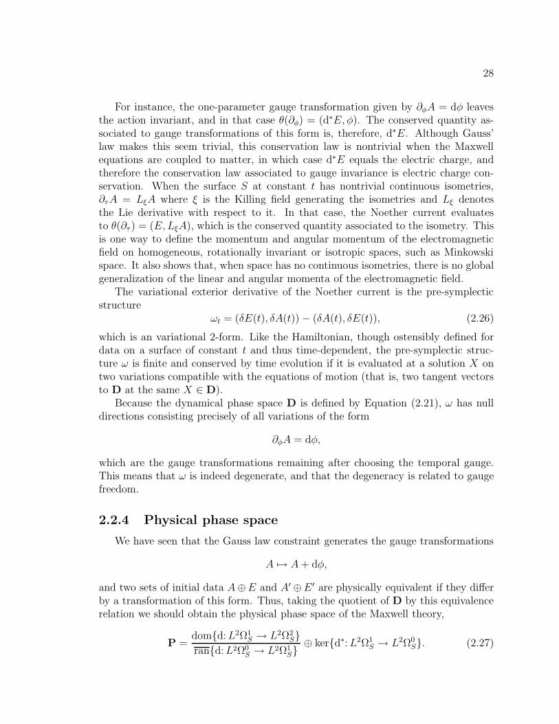
For instance, the one-parameter gauge transformation given by ∂φA = dφ leavesthe action invariant, and in that case θ(∂φ) = (d∗E, φ). The conserved quantity as-sociated to gauge transformations of this form is, therefore, d∗E. Although Gauss’law makes this seem trivial, this conservation law is nontrivial when the Maxwellequations are coupled to matter, in which case d∗E equals the electric charge, andtherefore the conservation law associated to gauge invariance is electric charge con-servation. When the surface S at constant t has nontrivial continuous isometries,∂τA = LξA where ξ is the Killing field generating the isometries and Lξ denotesthe Lie derivative with respect to it. In that case, the Noether current evaluatesto θ(∂τ ) = (E,LξA), which is the conserved quantity associated to the isometry. Thisis one way to define the momentum and angular momentum of the electromagneticfield on homogeneous, rotationally invariant or isotropic spaces, such as Minkowskispace. It also shows that, when space has no continuous isometries, there is no globalgeneralization of the linear and angular momenta of the electromagnetic field.

The variational exterior derivative of the Noether current is the pre-symplecticstructure

ωt = (δE(t), δA(t)) − (δA(t), δE(t)), (2.26)

which is an variational 2-form. Like the Hamiltonian, though ostensibly defined fordata on a surface of constant t and thus time-dependent, the pre-symplectic struc-ture ω is finite and conserved by time evolution if it is evaluated at a solution X ontwo variations compatible with the equations of motion (that is, two tangent vectorsto D at the same X ∈ D).

Because the dynamical phase space D is defined by Equation (2.21), ω has nulldirections consisting precisely of all variations of the form

∂φA = dφ,

which are the gauge transformations remaining after choosing the temporal gauge.This means that ω is indeed degenerate, and that the degeneracy is related to gaugefreedom.

2.2.4 Physical phase space

We have seen that the Gauss law constraint generates the gauge transformations

A 7→ A+ dφ,

and two sets of initial data A⊕E and A′ ⊕E ′ are physically equivalent if they differby a transformation of this form. Thus, taking the quotient of D by this equivalencerelation we should obtain the physical phase space of the Maxwell theory,

P =domd:L2Ω1

S → L2Ω2S

rand:L2Ω0S → L2Ω1

S⊕ kerd∗:L2Ω1

S → L2Ω0S. (2.27)

29

In words, the physical phase space consists of pairs [A]⊕E where: [A] is an equivalenceclass of square-integrable 1-forms on S with square-integrable exterior derivativesmodulo L2 limits of the exterior derivatives of square-integrable functions on S; and Eis a square-integrable 1-form on S with vanishing divergence.

Note that the Hamiltonian of Equation (2.25) is manifestly independent of anychoice of representative in the gauge equivalence class of A. On the other hand, the(now nondegenerate) symplectic structure (2.26) is gauge-independent only becauseof Gauss’ law, as

(A+ dβ,E) = (A,E) + (β, d∗E) = (A,E).

The first direct summand in Equation (2.27),

A =domd:L2Ω1

S → L2Ω2S

rand:L2Ω0S → L2Ω1

S,

has a natural Hilbert-space norm

‖[A]‖2A

= infφ∈Ω0

(A+ dφ,A+ dφ) + (dA, dA), (2.28)

which combines the natural norm on a quotient space with the natural Sobolev normon domd:L2Ω1

S → L2Ω2S. The second summand is simply

E = kerd∗:L2Ω1 → L2Ω0 with ‖E‖2E

= (E,E),

and the natural norm on P = A ⊕ E is the sum of the two. The Hamiltonian andsymplectic structure on P are continous with respect to these norms.

2.3 Free and oscillating modes

Since the definition of the physical phase space P is rather technical, let us ex-pound on it a bit. A point in the classical phase space is a pair [A] ⊕ E where: thevector potential [A] is an equivalence class of square-integrable 1-forms modulo gaugetransformations, with square-integrable exterior derivatives; and the electric field Eis a square-integrable 1-form satisfying the Gauss law. Our definition of the physicalphase space ensures that it contains precisely such pairs for which the Hamiltonian(physically, the energy) H is finite and the symplectic structure ω is well-defined.It also makes the gauge equivalence relation precise, and makes precise the sense inwhich the Gauss law holds.

Note that the physical phase space P does not necessarily contain all finite-energyinitial data for Maxwell’s equations, since we are imposing the additional conditionthat ([A], [A]) <∞ to make the symplectic structure well-defined. If we omitted thiscondition we could define a real Hilbert space consisting of all finite-energy initial data

30

for Maxwell’s equations, but the symplectic structure would only be densely definedon this space. This is a gauge-independent condition because ([A], [A]) smallest L2

norm among all the vector potentials in the same gauge-equivalence class; one couldfix the gauge by choosing the representative A such that (A,A) = ([A], [A]), but thatis not necessary.

Observe now that the phase space P and the Hamiltonian H are defined very sim-ply in terms of d and d∗, and recall the Kodaira orthogonal-direct-sum decomposition

L2Ω1S = rand0 ⊕ ker ∆1 ⊕ ran d∗

1

where ∆1 = d∗1d1 + d0d

∗0:L

2Ω1S → L2Ω1

S. We prove a general version of the Kodairadecomposition in Section 2.4. In the present section we use the decomposition towrite P as the direct sum of a part Pf containing the Aharonov–Bohm modes orfree modes, and a part Po containing the more familiar oscillating modes of theelectromagnetic field. We will see that it is convenient to treat the classical dynamicsof Maxwell theory separately on these two parts, but putting the results togetherwe shall see that time evolution acts as a strongly continuous 1-parameter groupof symplectic transformations on P. Note that, at least in the classical theory, theseparation of the oscillating and free modes is a matter of convenience.

Before embarking on the mathematical details of the Kodaira decomposition, letus explore its physical significance for the classical phase space of electromagnetism.

2.3.1 The space of pure-gauge potentials

Observe that, in our definition of the physical phase space, Equation (2.27), wehave taken the space of ‘pure gauge’ vector potentials to be ran d0. This is subtlydifferent from the common assumption that pure gauge potentials are derivatives ofarbitrary smooth scalar functions. Instead, we are saying they lie in the closure ofthe space of derivatives of square-integrable functions. While these nuances may seemmerely pedantic, they have have dramatic consequences in certain situations whichwe discuss in Section 4. The simplest example, in 2 + 1 dimensions, is when S is thehyperbolic plane, which has an infinite-dimensional space of square-integrable 1-formsthat are exterior derivatives of smooth functions which are not square-integrable, sothe 1-forms are not pure gauge by our definition.

Physically, as we are restricting the class of allowed gauge transformations (es-sentially to be compactly supported), in general there will be vector potentials thatwould naıvely be considered pure gauge but should not, because they involve a changeof gauge on an effectively infinite volume. However, these additional modes cannotbe detected by any experiment carried out on a finite volume, and so one could ar-gue that they should be discarded after all. However, these vector potentials arecanonically conjugate to static electric fields with finite energy, and so are required inthe canonical formulation of electromagnetism. This is even more important if theseelectric field modes are to be quantized.

31

Mathematically, our definition is natural thanks to the Kodaira decomposition,and it leads to consistent classical and quantum theories, except possibly (see chap-ters 4 and 6) in the case when the space of harmonic vector potentials is infinite-dimensional.

As for the electric field E, the space ran d0 is orthogonal to ker d∗0, so square-

integrable electric fields satisfying the Gauss’ law constraint d∗0E = 0 belong to ker ∆1⊕

ran d∗1.

2.3.2 Aharonov–Bohm modes

The space ker ∆1 consists of square-integrable harmonic 1-forms. For any vectorpotential A in this space, the magnetic field dA vanishes. If the manifold S is compact,Hodge’s theorem asserts that this space is isomorphic to the first de Rham cohomologyof S, a topological invariant, and vector potentials in this space can be detectedby their holonomies around noncontractible loops, as in the Aharonov–Bohm effect.Thus, in the compact case, it makes perfect sense to call ker ∆1 the configurationspace of ‘Aharonov–Bohm’ or ‘topological’ modes of the electromagnetic field.

The situation is subtler if S is noncompact. In this case ker ∆1 is called the‘first L2 cohomology group’ of S. The L2 cohomology of a non-compact Riemannianmanifold can differ from the de Rham cohomology, and it depends on the metric,so it is not a topological invariant. By analogy with the compact case we still callharmonic vector potentials ‘Aharonov–Bohm’ modes. As we shall see, sometimesthere are Aharonov–Bohm modes even when S is contractible. On the other hand,sometimes there are no Aharonov–Bohm modes when they would be expected onelementary topological considerations. Finally, the space of Aharonov–Bohm modesmay be infinite-dimensional. These facts make it a bit trickier to understand vectorpotentials in ker ∆ as topological Aharonov–Bohm modes. However, at least forcertain large classes of well-behaved manifolds, it still seems to be possible. Wereview some of these results in Section 4.

2.3.3 Decomposition into free and oscillating modes

We now apply the Kodaira decomposition to the physical phase space P, in orderto understand the Aharonov–Bohm modes more deeply, as well as the meaning of thethird summand ran δ1 in the Kodaira decomposition.

The Kodaira decomposition allows us write P as a direct sum Po⊕Pf of ‘oscillat-ing’ and ‘free’ modes of the electromagnetic field. The oscillating modes are familiarfrom electromagnetism on Minkowski spacetime. The free modes are those relevantto the Aharonov–Bohm effect; we call them ‘free’ because the equations of motion forthese modes are mathematically analogous to those of a free particle, as we shall see.

To see this in detail, first recall that

P = A ⊕E

32

whereA = dom d1/ ran d0

E = ker d∗1.

The Kodaira decomposition lets us split A and E into ‘oscillating’ and ‘free’ parts:

A ∼= Ao ⊕ Af

E = Eo ⊕ Ef ,

whereAo = dom d1 ∩ ran d∗

1 Af = ker ∆

Eo = rand∗1 Ef = ker ∆.

Note that the difference between Ao and Eo is coming from the different norms: ‖[A]‖2+‖dA‖2 versus ‖E‖2. This decomposition lets us write the classical phase space as adirect sum of real Hilbert spaces

P = Po ⊕ Pf ,

wherePo = Ao ⊕ Eo

Pf = Af ⊕ Ef .

This splitting respects the symplectic structure and also the Hamiltonian on P, sotime evolution acts independently on the oscillating and free part of any initial data[A] ⊕ E ∈ P.

2.3.4 The oscillating sector

For modes A⊕E ∈ Po, Maxwell’s equations say:∂tA = E∂tE = −∆A,

a generalization of the equations of motion for a harmonic oscillator. This is whywe call Po the phase space of ‘oscillating’ modes. The Hamiltonian on Po is also ofharmonic oscillator type:

H [A⊕ E] =1

2[(dA|dA) + (E|E)].

If we rewrite the above version of Maxwell’s equations as a single integral equation,we find it has solutions of the form

(AE

)7→ To(t)

(AE

)=

(cos(t

√∆) sin(t

√∆) /

√∆

−√

∆ sin(t√

∆) cos(t√

∆)

) (AE

)(2.29)

where we define functions of ∆ using the functional calculus [RS80]. The time evo-lution operators To(t) form a strongly continuous group of bounded operators on Po.This follows from three facts:

33

• ‖To(t)‖ is finite for all t.

• To(t)To(s) = To(t+s) for all real s, t. This involves simple formal manipulations(as if ∆ were a positive number) allowed by the functional calculus.

• limt→0 To(t)φ = φ for all φ ∈ Xo. This is a straightforward calculation.

2.3.5 The free sector

On the other hand, the space Pf consists of initial data where the vector potentialand electric field are harmonic; these are the states relevant to the Aharonov–Bohmeffect. For modes A⊕E ∈ Pf , Maxwell’s equations become

∂tA = E∂tE = 0

These are analogous to the equations of motion for a free particle on the line, with Aplaying the role of position and E playing the role of momentum. This is why wecall Pf the phase space of ‘free’ modes. The Hamiltonian on this space is also analo-gous to the kinetic energy of a free particle:

H [A⊕ E] =1

2(E | E).

Solving the equations of motion, we see that time evolution acts on Pf as follows:

(AE

)7→ Tf (t)

(AE

)=

(1 t0 1

) (AE

)(2.30)

The time evolution operators Tf (t) form a norm-continuous group of bounded oper-ators on Pf . Indeed:

• 1 ≤ ‖Tf (t)‖2 ≤ 2 + t2, so ‖Tf(t)‖ is finite for all t.

• Tf(t)Tf (s) = Tf (t+ s) for all real s, t, trivially.

• limt→0 Tf (t) = V (0) in the norm topology, since it is easily seen that ‖Tf(t) −Tf(0)‖ = |t|.

A key ingredient in these calculations is that (dA|dA) = 0 identically on Pf .

34

2.4 Summary

In this section we summarize the mathematical and physical content of the presentchapter in two results. The first, Theorem 5, gathers all the important analysis resultsconcerning the exterior derivative operator on square-integrable differential forms ona complete Riemannian manifold. The second, Result ?? describes the phase space ofvacuum electromagnetism in 3+1 dimensions as a real Hilbert space with a continuousquadratic and nonnegative Hamiltonian, and a continuous symplectic structure.

We can combine into a single theorem Gaffney’s Proposition 3 about the oper-ators d and δ on a complete Riemannian manifold and the version of the Kodairadecomposition (Proposition 6) which was essential to the physical interpretation ofthe phase space of Maxwell’s theory in the preceding section:

Theorem 5. Let S be a smooth manifold equipped with a complete Riemannian met-ric g. Then the formally adjoint operators

C∞0 Ωk

S

dk //C∞

0 Ωk+1S

d∗k

oo

have mutually adjoint closures

L2ΩkS

dk //L2Ωk+1

Sd∗

k

oo .

These closed operators satisfy

ran dk−1 ⊆ ker dk, ran d∗k ⊆ ker d∗

k−1

and there is a Hilbert-space direct-sum decomposition

L2Ωk = ran dk−1 ⊕ ker ∆k ⊕ ran δk.

where the Laplacian on k-forms,

∆k = δkdk + dk−1δk−1,

is a nonnegative densely defined self-adjoint operator on L2Ωk.

Proof. The properties of the operators d and d∗ are the subject of Section 2.1.3.We postpone proving the self-adjointness of the Laplacian to Corollary 15 in thenext chapter. To prove the desired direct sum decomposition, we apply the generalKodaira decomposition (Proposition 6 below) to

L2Ωk−1dk−1 //

L2Ωk

d∗k−1

oodk //

L2Ωk+1

d∗k

oo

35

and obtainL2Ωk = randk−1 ⊕ ker ∆k ⊕ ran d∗

k.

where∆k = d∗

kdk + dk−1d∗k−1

is the Laplacian on 1-forms.

It remains only to prove the following general form of the Kodaira decomposition,which is itself a generalization of the usual Hodge decomposition for differential formson a compact Riemannian manifold.

Proposition 6 (Kodaira decomposition). If

HS−−−→ H ′ T−−−→ H ′′

are densely defined closed operators and ranS ⊆ ker T , then

H ′ = ranT ∗ ⊕ ker(T ∗T + SS∗) ⊕ ranS.

Proof. We break the proof down into a series of lemmas. In the following results andproofs, all the spaces we will consider will be Hilbert spaces. The proofs work equallywell for real or complex Hilbert spaces, but in our application they will be real.

Lemma 7. If

HT−−−→ H ′

is a densely defined operator, then

ker T ∗ = (ranT )⊥ and ker T = (ranT ∗)⊥ ∩ domT.

Proof. Since (φ | Tψ)′ = (T ∗φ | ψ) for all φ ∈ domT ∗ and ψ ∈ domT , it followsthat ker T ∗ ⊥ ranT and ker T ⊥ ranT ∗. Since T is densely defined, (ranT )⊥ ⊆domT ∗.

The following lemma guarantees that the closed operators d and d∗ satisfy

ran dk−1 ⊆ ker dk, ran d∗k ⊆ ker dk−1.

Lemma 8. If

HS−−−→ H ′ T−−−→ H ′′

are densely defined operators and ranS ⊆ ker T , then

ranT ∗ ⊆ kerS∗.

Proof. Since ranS ⊆ ker T , for all φ ∈ domT ∗ and ψ ∈ domS we have

(T ∗φ | Sψ)′ = (φ | TSψ)′′ = (φ | 0)′′ = 0 = (0 | ψ),

so ranT ∗ ⊆ ker S∗.

36

Corollary 9. If

HS−−−→ H ′ T−−−→ H ′′

are densely defined closable operators and ranS ⊆ ker T , then

ranS ⊆ kerT .

Proof. By Lemma 2, since S, T are closable, S∗ and T ∗ are densely defined andS = S∗∗ and T = T ∗∗. Then, ranS ⊆ ker T implies ranT ∗ ⊆ kerS∗, so ranS∗∗ ⊆ker T ∗∗.

We are now ready to finish the proof of the Kodaira decomposition. The hypothe-ses of Proposition 6 guarantee that S∗ and T ∗ are densely defined closed operatorsand T = T ∗∗ and S = S∗∗ (Lemma 2), so

ker T = ker T ∗∗ = (ranT ∗)⊥ and kerS∗ = (ranS)⊥.

Then,H ′ = ker T ⊕ ranT ∗ = kerS∗ ⊕ ranS

which, together with the inclusions ranS ⊆ kerT and ranT ∗ ⊆ ker S∗ (Lemma 8),implies

H ′ = ranT ∗ ⊕ (ker T ∩ ker S∗) ⊕ ranS.

Finally, we know

(kerT ∩ kerS∗) ⊆ (ker(T ∗T ) ∩ ker(SS∗)) ⊆ ker(T ∗T + S∗S).

The result then follows from ker(T ∗T+S∗S) ⊆ (ker T∩ker S∗). Assume ψ ∈ ker(T ∗T+SS∗); then

(ψ | 0)′ = (ψ | (T ∗T + SS∗)ψ)′ = (ψ | T ∗Tψ)′ + (ψ | S∗∗S∗ψ)′

so that0 = (Tψ | Tψ)′′ + (S∗ψ | S∗ψ),

which implies ψ ∈ ker T ∩ ker S∗.

We end this chapter with a ‘physical theorem’ gathering all the results of physicalinterest about the phase space of electromagnetism that we proved in this chapter.

Result 10. Let M be a (3+1)-dimensional static, globally hyperbolic spacetime, withmetric

gM = e2Φ(−dt2 + g).

Then, electromagnetism on M with gauge group R has as its phase space the realHilbert space

P =domd:L2Ω1

S → L2Ω2S

rand:L2Ω0S → L2Ω1

S⊕ kerd∗:L2Ω1

S → L2Ω0S,

37

with continuous symplectic structure

ω(X,X ′) = (E,A′) − (E ′, A)

where X = [A] ⊕E and X ′ = [A′] ⊕E ′ lie in P, and

(α, β) =

∫

S

g(α, β)vol

is the canonical inner product induced on ΩkS by the optical metric g on S. The

Hamiltonian is the continuous quadratic form

H [X] =1

2[(E,E) + (dA, dA)].

There phase space splits naturally into two sectors,

P = Po ⊕ Pf ,

and the direct summands

Pf = P ∩ ker ∆ and Po = P ∩ ran d∗1

are preserved by time evolution. On Po, time evolution takes the form

(AE

)7→ To(t)

(AE

)=

(cos(t

√∆) sin(t

√∆) /

√∆

−√

∆ sin(t√

∆) cos(t√

∆)

) (AE

)

while on Pf it takes the form

(AE

)7→ Tf (t)

(AE

)=

(1 t0 1

) (AE

).

38

Chapter 3

p-form electromagnetism in n + 1

dimensions

In this chapter we generalize the results of the last chapter to electromagnetismon spacetimes of arbitrary dimension n + 1. As before, we take our spacetime to beof the form R × S, equipped with the Lorentzian metric

gM = e2Φ(−dt2 + g)

where g is a complete Riemannian metric on S. The only difference is that nowS is n-dimensional instead of 3-dimensional. However, this means that Maxwell’sequations are no longer conformally invariant, so the ‘gravitational potential’ Φ playsa more significant role. To see why, recall that the Maxwell action is still given by

S[AM ] = −1

2

∫

M

gM(FM , FM) volM

whereFM = dt ∧ (∂tA− dA0) + dA.

By Equation (2.6),

gM(FM , FM) = e−4Φ [−g(∂tA− dA0, ∂tA− dA0) + g(dA, dA)]

and, by Equation (2.3),volM = e(n+1)Φvol ∧ dt

where vol is the volume form on space. Hence, we have

S[A,A0] =1

2

∫

M

[g(∂tA− dA0, ∂tA− dA0) − g(dA, dA)] e(n−3)Φvol ∧ dt.

The factors involving Φ cancel only if n = 3, indicating conformal invariance. Inother dimensions, the most elegant way to deal with these factors involving Φ is toredefine the fields A0 and A by setting

AM = e−12(n−3)Φ(dt ∧ A0 + A),

39

and then to ‘twist’ the exterior derivative of differential forms on space, defining anew operator

D = e−12(n−3)Φ d e

12(n−3)Φ.

The action is then

S[A,A0] =1

2

∫

M

[g(∂tA−DA0, ∂tA−DA0) − g(DA,DA)]vol ∧ dt

which is formally just like equation (2.17) was in the (3 + 1)-dimensional case, butwith rescaled fields A and A0, and with the twisted exterior derivative D replacingthe usual d.

With the help of this formal equivalence, the whole theory goes through almostexactly as before. In particular, if we let L2Ωp be the Hilbert space consisting of allsquare-integrable p-forms on S, there are mutually adjoint operators

L2Ω0D0 //

L2Ω1

D∗0

ooD1 //

L2Ω2

D∗1

oo

Using the Kodaira decomposition for this sequence we obtain

L2Ω1 = ranD0 ⊕ kerL1 ⊕ ranD∗1

where now the Laplacian is replaced by the ‘twisted Laplacian’ L1, a nonnegativeself-adjoint operator on 1-forms given by

L1 = D∗1D1 +D0D

∗0.

In fact, having come this far, it would be a pity not to treat ‘p-form electromag-netism’, a generalization of Maxwell’s equations in which the electromagnetic vectorpotential is replaced by a p-form. The general case was treated by Henneaux andTeitelboim [HT86]. For p = 0, this theory is just the massless neutral scalar field.For p = 2, it is the Kalb–Ramond field arising naturally in string theory [GSW87,Section 3.4.5][KR74], while for p = 3 it plays a part in 11-dimensional supergravity[Duf99]. All our formulas generalize painlessly to these theories in the absence ofcharges. Starting with the p-form AM on spacetime, we define a field strength tensorFM = dMAM , and take the action of the theory to be

S[AM ] = −1

2

∫

M

gM(FM , FM) volM .

This action gives equations of motion and gauge symmetries having the same formas in Maxwell theory. Furthermore, if we set

AM = e−12(n−2p−1)Φ(dt ∧A0 + A)

40

and define the twisted differential D as follows:

D = e12(n−2p−1)Φde−

12(n−2p−1)Φ,

we obtain

S[A,A0] =1

2

∫

R

[(∂tA−DA0, ∂tA−DA0) − (DA,DA)]dt

in complete analogy with ordinary Maxwell theory. This allows us to generalize allour results on Maxwell’s equations to the p-form case.

41

3.1 Spacetime Geometry

We model spacetime as an (n+1)-dimensional smooth manifoldM with a Lorentzianmetric of signature (−+ · · ·+). We assume that M = R × S for some smooth mani-fold S, and that the metric on M is of the form

gM = −e2Φdt2 + gS

where gS is a Riemannian metric on S and Φ is a smooth real-valued function on S.As in Equation (2.2) we write

gM = e2Φ(−dt2 + g)

where the ‘optical metric’ g is given by g = e−2ΦgS. We assume that g makes S into acomplete Riemannian manifold, since this is a necessary and sufficient condition forMto be a globally hyperbolic spacetime with the surfaces t = c as Cauchy surfaces.For a more complete discussion, refer back to Section 2.1. As before, all fields onspacetime carry the subscript ‘M ’; fields on space are written without subscript orwith the subscript 0. To study p-form electromagnetism we need to fix an integer pwith 0 ≤ p ≤ n. Then, any k-form αM on M can be uniquely decomposed as

αM = e−12(n−2p−1)Φ(dt ∧ α0 + α)

where α is a time-dependent k-form on S and α0 a time-dependent (k−1)-form on S.As explained in the previous section, the strange-looking factor involving Φ is chosento simplify things later.

The metric gM induces a metric on the k-forms on spacetime, which we alsocall gM , and similarly for the metric g on space. In terms of spatial and temporalparts, these are related by:

gM(αM , α′M) = e−(n+2k−2p−1)Φ [−g(α0, β0) + g(α, β)] . (3.1)

Assuming that S is oriented, the metrics gM and g determine volume forms volMon M and vol on S, which are related by

volM = e(n+1)Φvol ∧ dt. (3.2)

Again, it would be possible to deal with the nonorientable case by working withdensities instead of forms. As before, we define an inner product (· | ·) on k-forms onspace by Equation (2.7), namely

(α, β) =

∫

S

g(α, β) vol,

and define L2Ωk to be the space of measurable k-forms α on S such that (α | α) <∞.

42

We define the twisted exterior derivative Dk:C∞0 Ωk

S → C∞0 Ωk+1

S by

Dk = e12(n−2p−1)Φdke

− 12(n−2p−1)Φ. (3.3)

This operator has a formal adjoint

D†k = e−

12(n−2p−1)Φδk+1e

12(n−2p−1)Φ (3.4)

meaning that(D†

kα, β) = (α,Dkβ) (3.5)

whenever α ∈ C∞0 Ωk+1 and β ∈ C∞

0 Ωk. In what follows we shall omit the subscript ‘k’from the operators Dk and D†

k when it is clear from context.In Section (3.3) we shall show that these operators have mutually adjoint clo-

sures Dk:L2Ωk

S → L2Ωk+1S and D∗

k:L2Ωk+1

S → ΩkS, and that the operators DkD

†k

andD†kDk are both essentially self-adjoint, meaning that their respective closures,DkD

∗k

and D∗kDk, are their unique self-adjoint extensions [RS80, §VIII.2].

3.2 p-Form electromagnetism

In p-form electromagnetism we take the vector potential as a p-form on space-time, AM , and take the action to be

S[AM ] = −1

2

∫

M

gM(FM , FM) volM

where the field strength tensor FM is given by

FM = dMAM

In terms of the twisted exterior derivative defined in Equation (3.3), the field strengthtensor equals

FM = (dt ∧ ∂t + d)AM

= (dt ∧ ∂t + d)e−12(n−2p−1)Φ(dt ∧ A0 + A)

= e−12(n−2p−1)Φ(dt ∧ ∂t +D)(dt ∧ A0 + A)

= e−12(n−2p−1)Φ[dt ∧ (∂tA−DA0) +DA].

With the help of equations (3.1)–(3.2), this means that the action can be written as

S =1

2

∫

R

∫

M

[g(∂tA−DA0, ∂tA−DA0) − g(DA,DA)]volM

=1

2

∫

R

[(∂tA−DA0, ∂tA−DA0) − (DA,DA)] dt. (3.6)

43

Note the complete analogy with Equation (2.17). This action gives the followingequations of motion:

∂tDA = DA0

∂2tA = −D†DA+ ∂tDA0.

The equations of p-form electromagnetism admit gauge symmetries of the form

AM 7→ AM + dMβM

where βM is a (p − 1)-form on spacetime. Thus, to obtain evolution equations, wework in temporal gauge, which amounts to setting A0 = 0. The above equations canthen be written as

D†E = 0∂tA = E∂tE = −D†DA.

The Gauss law constraint D†E = 0 generates gauge transformations of the form

A 7→ A +Dβ

where β is a (p− 1)-form on spacetime. Two pairs A⊕E are physically equivalent ifthey differ by such a transformation. Thus, ignoring analytical subtleties, the phasespace of p-form electromagnetism consists of pairs [A]⊕E where [A] is an equivalenceclass of p-forms on S modulo those of the form Dβ (twisted-exact), and E is a p-formon S satisfying D†E = 0 (twisted-divergenceless). The Hamiltonian on this phasespace is easily seen to be

H [[A] ⊕ E] =1

2[(DA,DA) + (E,E)].

and the symplectic structure is

ω[[A] ⊕ E, [A′] ⊕ E ′] = (A,E ′) − (E,A′).

Again as in the case of 3 + 1 dimensions, (Dβ,E) = (β,D†E) = 0 implies that thesymplectic structure is gauge-invariant.

All these formulas have analogues in Section 2, so to generalize all the results ofthat section we only need to generalize Theorem 5 to the present context. In otherwords, first we must show that the operators

C∞0 Ωk

D //C∞

0 Ωk+1

D†

oo

have mutually adjoint closures, which we write as

L2ΩkD //

L2Ωk+1

D∗oo .

44

Then we must prove a version of the Kodaira decomposition saying that

L2Ωp = ranDp−1 ⊕ kerLp ⊕ ranD∗p

where the twisted Laplacian on k-forms,

Lp = D∗pDp +Dp−1D

∗p−1,

is a nonnegative self-adjoint operator on L2Ωp. We do all this in Section 3.3 below.Using these facts, we define the classical phase space for p-form electromagnetism

to beP = A ⊕E

whereA = domDp/ ranDp−1

E = kerDp.

As with the Maxwell theory in 3+1 dimensions, P becomes a real Hilbert space spaceif we define

‖[A] ⊕E‖2 = ([A], [A]) + (dA, dA) + (E | E),

where ([A], [A]′) can be defined on gauge equivalence classes using the fact that, by theKodaira decomposition, L2Ωp/ranDp−1 is canonically isomorphic to ranD⊥

p , whichinherits an inner product by virtue of being a subspace of L2Ωp.

As before, we can split the spaces A and E into ‘oscillating’ and ‘free’ parts:

A = Ao ⊕ Af

E = Eo ⊕ Ef ,

whereAo = domDp ∩ ranD∗

p Af = kerLp

Eo = ranD∗p Ef = kerLp.

These decompositions let us write the classical phase space as a direct sum of realHilbert spaces:

P = Po ⊕ Pf ,

wherePo = Ao ⊕ Eo

Pf = Af ⊕ Ef .

This is also a direct sum of symplectic vector spaces, and the Hamiltonian is a sumof separate Hamiltonians on Po and Pf . As a result, time evolution acts by sym-plectic transformations, independently on the oscillating and free parts of any initialdata [A] ⊕E ∈ P.

45

For modes [A]⊕E ∈ Po, the Hamiltonian resembles that of a harmonic oscillator:

H [A⊕ E] =1

2[(DA,DA) + (E,E)]

and the equations of motion are

∂tA = E∂tE = −LA,

where we write the twisted Laplacian Lp simply as L. The solutions of the corre-sponding integral equation are given by

(AE

)7→

(cos(t

√L) sin(t

√L) /

√L

−√L sin(t

√L) cos(t

√L)

) (AE

)(3.7)

where we use the functional calculus to define functions of L. The proof that this is astrongly continuous 1-parameter group of bounded operators is essentially the sameas the one sketched after Equation (2.29).

For modes [A] ⊕E ∈ Pf , the Hamiltonian resembles that of a free particle:

H [[A] ⊕ E] =1

2(E,E)

and the equations of motion are

∂tA = E∂tE = 0.

The solutions of the equations of motion are given by

(AE

)7→

(1 t0 1

) (AE

)

Note that, in the case of free modes, nothing besides the definition of the Laplacianhas changed from the case of 1-forms in 3+1 dimensions. In particular, time evolutionis given by the very same Equation (2.30).

3.3 Mathematical details

The results we need to make our work in the previous section rigorous are allcontained in this theorem:

46

Theorem 11. Let S be a smooth n-dimensional manifold equipped with a completeRiemannian metric g, and let Φ be a smooth real-valued function on S. Fix an integer0 ≤ p ≤ n. Then for any integer k, the operators

C∞0 Ωk

S

Dk //C∞

0 Ωk+1S

D†k

oo

defined in equations (3.3) and (3.4) have mutually adjoint closures, which we writeas

L2ΩkS

Dk //L2Ωk+1

SD∗

k

oo

These closures satisfy

ranDk−1 ⊆ kerDk, ranD∗k ⊆ kerD∗

k−1,

and we obtain a direct sum decomposition

L2Ωk = ranDk−1 ⊕ kerLk ⊕ ranD∗k.

where the twisted Laplacian on k-forms,

Lk = D∗kDk +Dk−1D

∗k−1,

is a nonnegative densely defined self-adjoint operator on L2Ωk.

Proof. Because of the twisting of the exterior derivative operator in Equation (3.3),one cannot simply apply the proof of Theorem 5. The reason is that Gaffney’s Propo-sition 3 depends on the specific properties of the ‘untwisted’ d and δ. However, thegeneralization is in fact true, essentially because efde−f and d have the same first-order part whenever f is a smooth function. This is made precise by an argument dueto Chernoff, which uses the concept of the ‘symbol’ of a differential operator. Thisargument implies both a generalization of Proposition 3 and the self-adjointness ofthe twisted Laplacian.

We begin by recalling Chernoff’s formalism [Che73], which is the key to provingthis theorem. Let S be a Riemannian manifold with metric g, and let E be any vectorbundle on S whose fiber at each point x ∈ S is equipped with an inner product 〈·, ·〉xdepending smoothly on x. The space of smooth compactly supported sections of thisvector bundle, denoted C∞

0 E, is given an inner product

(α | β) =

∫

S

〈α(x), β(x)〉x volS,

where volS is the canonical volume form on S. The Hilbert space completion of C∞0 E

with respect to this inner product is denoted L2E.

47

Assume that T :C∞0 E → C∞

0 E is a first-order linear differential operator on E. Itsformal adjoint T † is again a first-order linear differential operator, defined by requiringthat

(α | Tβ) = (T †α | β) for all α, β ∈ C∞0 E.

The ‘symbol’ of T is defined by

σ(df, α) = T (fα) − fTα

for any C∞0 function f and any α ∈ C∞

0 E. Note that σ(df, α) is a function on Swhose value at any point depends only on the values of df and α at that point.

If T + T † is equal to multiplication by a smooth function, we say the differentialequation ∂tα = Tα is a ‘symmetric hyperbolic system’. At any point x ∈ S, solutionsof this equation propagate at the speed

c(x) = sup‖σ(df, α)‖x: ‖df‖x = ‖α‖x = 1

where ‖df‖x is the norm of df at the point x, defined using the Riemannian metric g,and ‖α‖x is the norm of α at the point x, defined using the inner product on the fiberof E at x.

Chernoff then essentially proves the following theorem. Note that the Hilbertspaces appearing in this theorem are complex, so to apply it to our real Hilbertspaces we need to complexify them.

Lemma 12 (Chernoff). If the metric c−2g makes S into a complete Riemannianmanifold, the symmetric hyperbolic system ∂tα = Tα with initial data in C∞

0 E has aunique solution on R × S which is in C∞

0 E for all t ∈ R. Moreover, if T is formallyskew-adjoint (T + T † = 0), then −iT and all its powers are essentially self-adjointon C∞

0 E.

Sketch of proof. The basic idea is that when we solve the differential equation ∂tα =Tα, perturbations propagate at speed 1 with respect to the metric c−2g. If this metricis complete, information can never reach spacelike infinity in a finite amount of time.Thus, given compactly supported smooth initial data, the equation ∂tα = Tα hasa solution α(t, x) such that α(t, ·) is compactly supported for all t—and smooth, bygeneral results on hyperbolic systems.

If T is formally skew-adjoint, one can show that the inner product of two solutionsis constant as a function of time:

ddt

(α(t, ·) | β(t, ·)) = (Tα(t, ·) | β(t, ·)) + (α(t, ·) | Tβ(t, ·))= (α(t, ·) | T †β(t, ·)) + (α(t, ·) | Tβ(t, ·))= 0.

The crucial point here is that α(t, ·) and β(t, ·) are compactly supported for all t,so there are no boundary terms: we only need the fact that T and T † are formaladjoints.

48

It follows that time evolution defines a one-parameter group of inner-product-preserving transformations of C∞

0 E, which by density extends uniquely to a one-parameter unitary group U(t) on L2E. One can show that C∞

0 E forms a ‘denseinvariant subspace of C∞ vectors’ for U(t); in other words, that C∞

0 E is a densesubspace of L2E, and that given initial data α in this subspace, the solution U(t)αremains in this subspace for all times, defining an infinitely differentiable functionfrom R to L2E. By a theorem of Nelson [Nel59, Lemma 10.1], this implies that −iTand all its powers are essentially self-adjoint on the domain C∞

0 E, and that the closureof −iT generates the one-parameter group U(t). The only new thing to check hereis the existence of the derivatives dn

dtnU(t)α, which one can show by repeatedly using

the differential equation ddtU(t)α = −iTU(t)α.

This result applies without modification to first-order differential equations likethe Dirac equation. To apply it to our problem, we resort to a well-known trick,taking −iT to be the operator (

0 D†k

Dk 0

).

The essential self-adjointness of this operator will imply thatDk andD†k have mutually

adjoint closures:

Lemma 13. Let H1 and H2 be Hilbert spaces and let

H1

A // H2B

oo

be densely defined operators that are formal adjoints of one another:

〈Aφ, ψ〉1 = 〈φ,Bψ〉2 for all φ ∈ domA,ψ ∈ domB.

Let H = H1 ⊕H2 and let S be the densely defined operator

(0 BA 0

)

on H. If S is essentially self-adjoint, then A and B have mutually adjoint closures.

Proof. It is easy to verify that the closure of S is

(0 BA 0

)

while the adjoint of the closure of S is

(0 (A)∗

(B)∗ 0

).

49

If S is essentially self-adjoint, these two operators are equal. This implies that

(A)∗ = B

and(B)∗ = A

so the closures of A and B are mutually adjoint.

Lemma 14. Suppose S is a complete Riemannian manifold and Φ a smooth real-valued function on S. Let

T :L2ΩkS ⊕ L2Ωk+1

S → L2ΩkS ⊕ L2Ωk+1

S

be the densely defined operator

(0 iD†

k

iDk 0

).

Then −iT and all its powers are essentially self-adjoint on C∞0 Ωk ⊕ C∞

0 Ωk+1.

Proof. We show that the hypotheses of Lemma 12 apply to the operator T . ClearlyT is formally skew-adjoint, so it suffices to check that the equation ∂tα = Tα haspropagation speed c = 1.

First we consider the case where Φ = 0, so D = d and D† = δ. The symbol of theoperator d is

σd(df, α) = (d(fα) − fdα) = df ∧ αfor any α ∈ C∞

0 ΩpS . The symbol of δ is

σδ(df, β) = −idfβ for any β ∈ C∞0 Ωp+1

S ,

since

(σδ(df, β), γ) = (δ(fβ) − fδβ, γ) = −(β, d(fγ) − fdγ) = −(β, df ∧ γ) = −(idfβ, γ)

for any γ ∈ C∞0 Ωp

S. It follows that the symbol of T is

σT (df, α⊕ β) = i(idhβ ⊕ df ∧ α).

To compute the propagation speed, note first that

‖σ(df, α⊕ β)‖2x = ‖df ∧ α‖2

x + ‖idfβ‖2x

≤ ‖df‖2 (‖α‖2x + ‖β‖2

x)= ‖df‖2 (‖α⊕ β‖2

x)

50

so the propagation speed is ≤ 1. In fact the propagation speed is exactly 1, sinceequality is achieved by letting df = dx1, α = dx2 ∧ · · · ∧ dxk+1, and β = 0 near x,where dx1, . . . , dxn is a coordinate frame orthogonal at x.

To deal with the general case where Φ is nonzero, note that for any first-orderlinear differential operator X and any smooth real-valued function h, the operatorehXe−h has the same symbol as X. In particular, the operators d and D have thesame symbol, as do δ and D†. It follows that T always has the same symbol as itdoes in the special case where Φ = 0, so the propagation speed is always 1.

Corollary 15. Under the same hypothesis as Lemma 14, the operators

C∞0 Ωk

S

Dk //C∞

0 Ωk+1S

D†k

oo

have mutually adjoint closures, and the operators D†kDk and DkD

†k−1 are essentially

self-adjoint on C∞0 Ωk.

Proof. The first part follows immediately from Lemmas 13 and 14. For the secondpart, note by Lemma 14 that T 2 = D†

kDk⊕DkD†k is essentially self-adjoint on C∞

0 Ωk⊕C∞

0 Ωk+1. This implies that D†kDk and DkD

†k are essentially self-adjoint.

We can now complete the proof of Theorem 11.If we now use Dk and D∗

k to stand for the mutually adjoint closures of the opera-tors Dk and D†

k, Lemma (8) implies that

ranDk−1 ⊆ kerDk, ranD∗k ⊆ kerD∗

k−1,

so we can apply the Kodaira decomposition (Proposition 6) to see that

L2Ωk = ranDk−1 ⊕ kerLk ⊕ ranD∗k.

whereLk = D∗

kDk +Dk−1D∗k−1.

To conclude we only need to show that Lk is a non-negative self-adjoint operator.With respect to the Kodaira decomposition this operator takes the block diagonalform

Dk−1D

∗k−1 0 0

0 0 00 0 D∗

kDk

.

It thus suffices to show that that D∗kDk and Dk−1D

∗k−1 are nonnegative and self-

adjoint. By Lemma 14 we know these operators are essentially self-adjoint whenrestricted to C∞

0 Ωk. So all that remains is to show that they are nonnegative. But(x | D∗

kDkx) = (Dkx | Dkx) ≥ 0 for all x ∈ domD∗kDk.

51

We end this section with a ‘physical theorem’ entirely analogous to the Result 10stated at the end of last chapter.

Result 16. Let M be a (n+1)-dimensional static globally hyperbolic spacetime, withmetric

gM = e2Φ(−dt2 + g).

Then, p-form electromagnetism on M with gauge group R has as its phase space thereal Hilbert space

P =domDp:L

2ΩpS → L2Ωp+1

S ranDp−1:L2Ωp−1

S → L2ΩpS

⊕ kerD∗p−1:L

2ΩpS → L2Ωp−1

S ,

whereDp = e

12(n−2p−1)Φdpe

− 12(n−2p−1)Φ

is the twisted exterior derivative. The phase space admits a continuous symplecticstructure

ω(X,X ′) = (E,A′) − (E ′, A)

where X = [A] ⊕E and X ′ = [A′] ⊕E ′ lie in P and

(α, β) =

∫

S

g(α, β)vol

is the canonical inner product induced on ΩkS by the optical metric g on S. The

Hamiltonian is the continuous quadratic form

H [X] =1

2[(E,E) + (DpA,DpA)].

The phase space splits naturally into two sectors,

P = Po ⊕ Pf ,

and the direct summands

Pf = P ∩ kerL and Po = P ∩ ranD∗p

are preserved by time evolution. On Po, time evolution takes the form(AE

)7→ To(t)

(AE

)=

(cos(t

√Lp) sin(t

√Lp) /

√Lp

−√Lp sin(t

√Lp) cos(t

√Lp)

) (AE

)

while on Pf it takes the form(AE

)7→ Tf (t)

(AE

)=

(1 t0 1

) (AE

).

52

Chapter 4

Hodge–de Rham theory onnoncompact manifolds

As we have seen, the space of harmonic differential forms, consisting of closed andcoclosed differential forms, plays a special role in the analysis of the phase space ofMaxwell’s equations: it corresponds to the space of physical vector potentials withvanishing magnetic field (Aharonov–Bohm effect), and also to static electric fieldswith no finite sources (charge without charge).

When space is compact, it is well known that the Hodge-de Rham theorem iden-tifies the square-integrable, smooth and real cohomologies of a space, and that thespace of square-integrable harmonic forms coincides with the kernel of the HodgeLaplacian ∆ = dδ + δd.

When space is noncompact everything becomes more complicated. To begin with,the definition of the codifferential δ involves integration by parts. As a result, unlessspace is complete in the optical metric it may be impossible to define the codifferential(and hence the Laplacian) without specifying boundary conditions at infinity. Whenthe optical metric on space is complete, not only is there an unambiguous definition ofthe codifferential and Laplacian, but the space of L2 harmonic forms is identified withthe kernel of the Hodge Laplacian, and it has a square-integrable cohomology inter-pretation. However, the square-integrable cohomology is not a topological invariant,as it depends crucially on the geometry at infinity.

These are the main questions one can ask about the Laplacian ∆ on a completeRiemannian manifold [Lot97, Car01, Car02]:

1. Is the dimension of ker ∆p finite or infinite? In physical terms, this is thedimension of the space of p-form Aharonov–Bohm modes.

2. What are sufficient conditions for ker ∆p to be trivial or finite-dimensional?

3. If ker ∆p is finite-dimensional, does it have a topological interpretation?

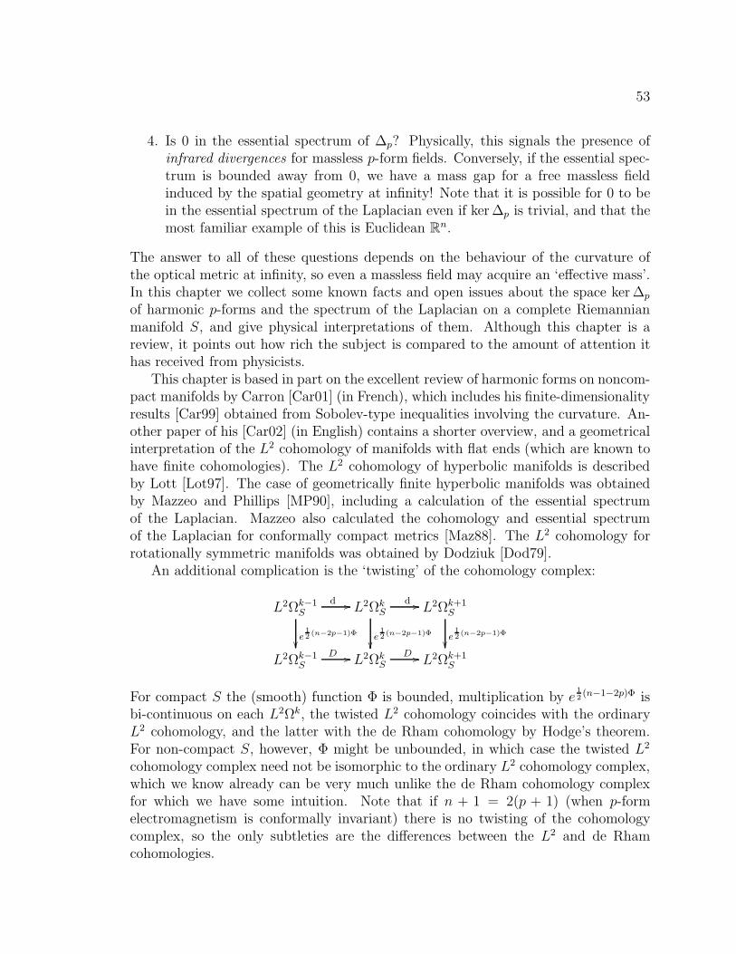
53

4. Is 0 in the essential spectrum of ∆p? Physically, this signals the presence ofinfrared divergences for massless p-form fields. Conversely, if the essential spec-trum is bounded away from 0, we have a mass gap for a free massless fieldinduced by the spatial geometry at infinity! Note that it is possible for 0 to bein the essential spectrum of the Laplacian even if ker ∆p is trivial, and that themost familiar example of this is Euclidean Rn.

The answer to all of these questions depends on the behaviour of the curvature ofthe optical metric at infinity, so even a massless field may acquire an ‘effective mass’.In this chapter we collect some known facts and open issues about the space ker ∆p

of harmonic p-forms and the spectrum of the Laplacian on a complete Riemannianmanifold S, and give physical interpretations of them. Although this chapter is areview, it points out how rich the subject is compared to the amount of attention ithas received from physicists.

This chapter is based in part on the excellent review of harmonic forms on noncom-pact manifolds by Carron [Car01] (in French), which includes his finite-dimensionalityresults [Car99] obtained from Sobolev-type inequalities involving the curvature. An-other paper of his [Car02] (in English) contains a shorter overview, and a geometricalinterpretation of the L2 cohomology of manifolds with flat ends (which are known tohave finite cohomologies). The L2 cohomology of hyperbolic manifolds is describedby Lott [Lot97]. The case of geometrically finite hyperbolic manifolds was obtainedby Mazzeo and Phillips [MP90], including a calculation of the essential spectrumof the Laplacian. Mazzeo also calculated the cohomology and essential spectrumof the Laplacian for conformally compact metrics [Maz88]. The L2 cohomology forrotationally symmetric manifolds was obtained by Dodziuk [Dod79].

An additional complication is the ‘twisting’ of the cohomology complex:

L2Ωk−1S

d //

e12 (n−2p−1)Φ

L2ΩkS

d //

e12 (n−2p−1)Φ

L2Ωk+1S

e12 (n−2p−1)Φ

L2Ωk−1S

D // L2ΩkS

D // L2Ωk+1S

For compact S the (smooth) function Φ is bounded, multiplication by e12(n−1−2p)Φ is

bi-continuous on each L2Ωk, the twisted L2 cohomology coincides with the ordinaryL2 cohomology, and the latter with the de Rham cohomology by Hodge’s theorem.For non-compact S, however, Φ might be unbounded, in which case the twisted L2

cohomology complex need not be isomorphic to the ordinary L2 cohomology complex,which we know already can be very much unlike the de Rham cohomology complexfor which we have some intuition. Note that if n + 1 = 2(p + 1) (when p-formelectromagnetism is conformally invariant) there is no twisting of the cohomologycomplex, so the only subtleties are the differences between the L2 and de Rhamcohomologies.

54

Since the twisted Laplacian DD∗ +D∗D has not been studied in nearly as muchdetail as the ordinary Hodge Laplacian, we know little about its behaviour. Therefore,when Φ is unbounded, most of what we will say in this chapter is directly applicableonly to the cases where p-form electromagnetism is conformally invariant—i.e., p-formelectromagnetism in 2(p+1)-dimensional spacetime, which includes the classical caseof 1-forms in 3 + 1 dimensions.

55

4.1 Cohomologies galore

Let C∞ΩkS denote the space of smooth k-forms on space. The exterior derivative

d:C∞ΩkS → C∞Ωk+1

S

gives rise to the smooth (de Rham) complex

C∞Ωk−1S

d // C∞ΩkS

d // C∞Ωk+1S

and the smooth de Rham cohomology is

Hk(S): =Zk(S)

Bk(S): =

kerd:C∞ΩkS → C∞Ωk+1

S dC∞Ωk−1

S

.

It is the content of de Rham’s theorem that Hk(S) is isomorphic to the real cohomol-ogy of the manifold, Hk(S; R).

Recall that we used compactly-supported smooth differential forms to derive theMaxwell equations. Denoting the space of smooth, compactly-supported k-formsby C∞

0 ΩkS, we have the complex

C∞0 Ωk−1

Sd // C∞

0 ΩkS

d // C∞0 Ωk+1

S

and the compactly-supported smooth cohomology is defined by

Hk0 (S): =

Zk0 (S)

Bk0 (S)

: =kerd:C∞

0 ΩkS → C∞

0 Ωk+1S

dC∞0 Ωk−1

S

.

If S is the interior of a compact manifold M with boundary ∂M , then Hk0 (S) is

isomorphic to the real relative cohomology of M , denoted Hk(M, ∂M ; R).In fact, the derivation of the Maxwell equations and the definition of the codiffer-

ential δ required an inner product on the space of differential forms. If L2ΩkS denotes

the space of square-integrable k-forms on S, then we have the complex

L2Ωk−1S

d // L2ΩkS

d // L2Ωk+1S

where d is the densely-defined operator obtained by closing the exterior differentialdefined on compactly-supported, smooth differential forms. The reduced L2 coho-mology is

Hk2 (S): =

Zk2 (S)

Bk2 (S)

: =kerd:L2Ωk

S → L2Ωk+1S

dL2Ωk−1S

.

and has a natural Hilbert-space topology. Note also that dL2Ωk−1S = dC∞

0 Ωk−1S . This

cohomology space is not a topological invariant, but it is quasi-isometrically invariant,

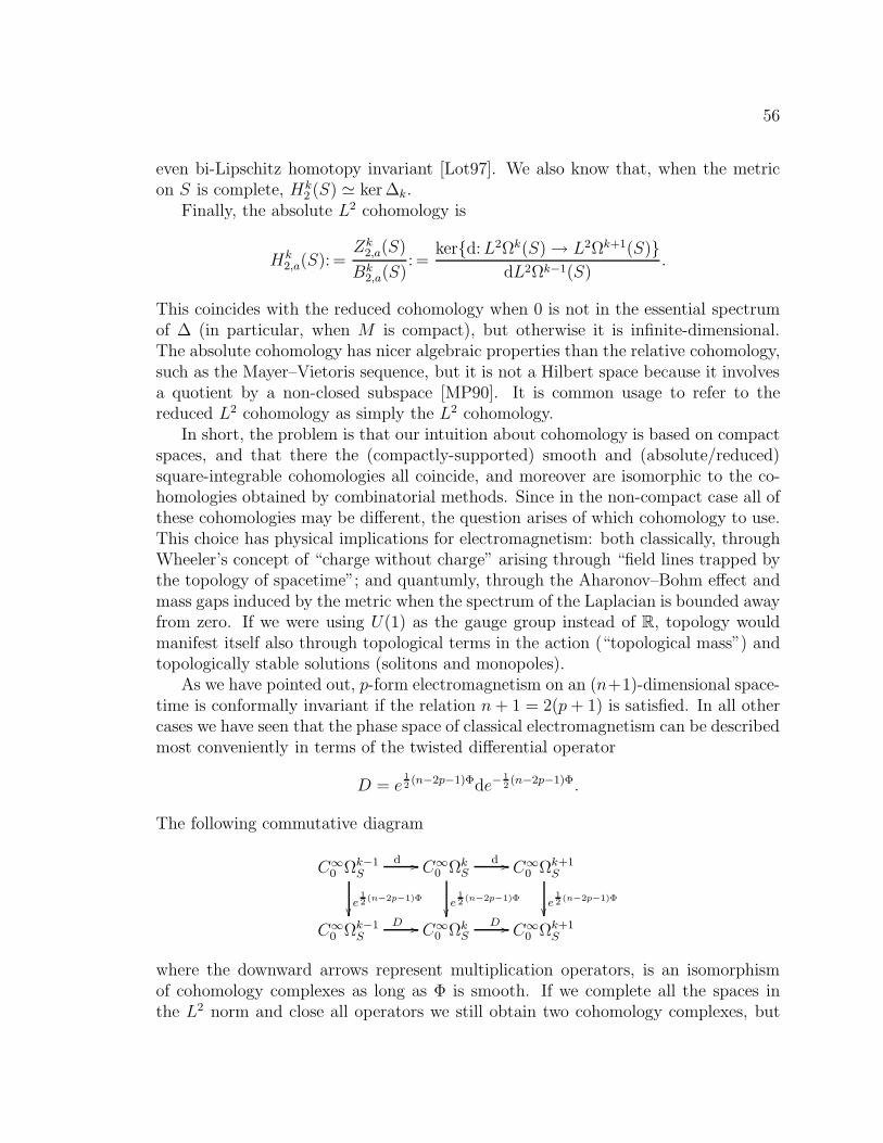
56

even bi-Lipschitz homotopy invariant [Lot97]. We also know that, when the metricon S is complete, Hk

2 (S) ≃ ker ∆k.Finally, the absolute L2 cohomology is

Hk2,a(S): =

Zk2,a(S)

Bk2,a(S)

: =kerd:L2Ωk(S) → L2Ωk+1(S)

dL2Ωk−1(S).

This coincides with the reduced cohomology when 0 is not in the essential spectrumof ∆ (in particular, when M is compact), but otherwise it is infinite-dimensional.The absolute cohomology has nicer algebraic properties than the relative cohomology,such as the Mayer–Vietoris sequence, but it is not a Hilbert space because it involvesa quotient by a non-closed subspace [MP90]. It is common usage to refer to thereduced L2 cohomology as simply the L2 cohomology.

In short, the problem is that our intuition about cohomology is based on compactspaces, and that there the (compactly-supported) smooth and (absolute/reduced)square-integrable cohomologies all coincide, and moreover are isomorphic to the co-homologies obtained by combinatorial methods. Since in the non-compact case all ofthese cohomologies may be different, the question arises of which cohomology to use.This choice has physical implications for electromagnetism: both classically, throughWheeler’s concept of “charge without charge” arising through “field lines trapped bythe topology of spacetime”; and quantumly, through the Aharonov–Bohm effect andmass gaps induced by the metric when the spectrum of the Laplacian is bounded awayfrom zero. If we were using U(1) as the gauge group instead of R, topology wouldmanifest itself also through topological terms in the action (“topological mass”) andtopologically stable solutions (solitons and monopoles).

As we have pointed out, p-form electromagnetism on an (n+1)-dimensional space-time is conformally invariant if the relation n+ 1 = 2(p+ 1) is satisfied. In all othercases we have seen that the phase space of classical electromagnetism can be describedmost conveniently in terms of the twisted differential operator

D = e12(n−2p−1)Φde−

12(n−2p−1)Φ.

The following commutative diagram

C∞0 Ωk−1

Sd //

e12 (n−2p−1)Φ

C∞0 Ωk

Sd //

e12 (n−2p−1)Φ

C∞0 Ωk+1

S

e12 (n−2p−1)Φ

C∞0 Ωk−1

SD // C∞

0 ΩkS

D // C∞0 Ωk+1

S

where the downward arrows represent multiplication operators, is an isomorphismof cohomology complexes as long as Φ is smooth. If we complete all the spaces inthe L2 norm and close all operators we still obtain two cohomology complexes, but

57

the diagram

L2Ωk−1S

d //

e12 (n−2p−1)Φ

L2ΩkS

d //

e12 (n−2p−1)Φ

L2Ωk+1S

e12 (n−2p−1)Φ

L2Ωk−1S

D // L2ΩkS

D // L2Ωk+1S

now has vertical arrows which, depending on the behaviour of Φ and dΦ at spatialinfinity, may be only densely defined, and so definitely not isomorphisms. Therefore,the ordinary (top) and twisted (bottom) chain complexes may not be isomorphic, andso the ‘twisted’ L2 cohomology based on D may not be isomorphic to the ordinaryone based on d, even though the smooth cohomologies are in fact isomorphic.

This may come about in several ways. On the one hand, the closure of themultiplication operator depends on the behaviour of the function Φ at infinity. In-

deed, for a k-form α to be in the domain of e12(n−1−2p)Φ it is necessary that both α

and e12(n−1−2p)Φα be square-integrable. Also, although multiplication by e

12(n−1−2p)Φ

is an isomorphism between spaces of smooth forms, its closure need not be invertibleif Φ is unbounded. On the other hand, the closure of D = d + [p + 1 − n+1

2](dΦ)∧

depends on the behaviour of dΦ at infinity, which can be wild even if Φ is bounded.

4.2 Known results

In this section we present a summary of known results on the (reduced) L2 co-homology of a Riemannian manifold. Since Poincare duality still holds in the formHk

2 (S) ≃ Hn−k2 (S), so only the cases 0 ≤ 2k ≤ n need be considered.

The zeroth cohomology H02 (S) is 1-dimensional if S has finite volume, and trivial

otherwise. This is easy to understand since, essentially, the question is whetherconstants are square-integrable or not. This is the first difference with the compactcase.

Other than in the extreme dimensions 0 and n, very little can be said in general.For instance, Anderson [And85] proves that, if n > 1, a > |n− 2p| and a ≥ 1, thereare complete Riemannian manifolds diffeomorphic to Rn, with curvature boundedby −a2 ≤ K ≤ 1 and such that their pth square-integrable cohomology Hp

2 is infinite-dimensional.

For rotationally symmetric n-dimensional manifolds with metric

ds2 = dr2 + f(r)2dθ2,

where dθ is the standard metric on Sn−1, the square-integrable cohomology is Hk2 =

0 if k 6= 0, n/2, n. As we know, when k = 0, n the cohomology depends on thevolume of spacetime. Finally, when k = n/2, Hk

2 = 0 if∫ ∞ ds

f(s)= ∞, and infinite-

dimensional otherwise. This is because of conformal invariance of the cohomology inthe middle dimension, and the fact that convergence of the integral correlates with

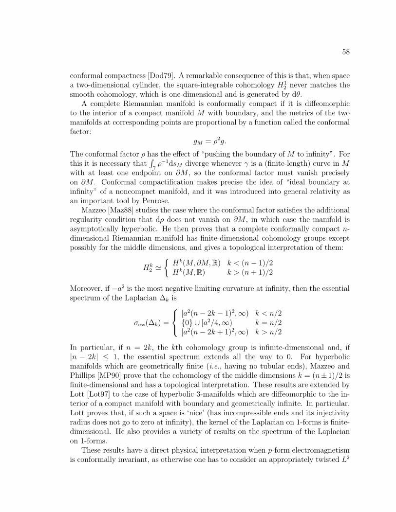
58

conformal compactness [Dod79]. A remarkable consequence of this is that, when spacea two-dimensional cylinder, the square-integrable cohomology H1

2 never matches thesmooth cohomology, which is one-dimensional and is generated by dθ.

A complete Riemannian manifold is conformally compact if it is diffeomorphicto the interior of a compact manifold M with boundary, and the metrics of the twomanifolds at corresponding points are proportional by a function called the conformalfactor:

gM = ρ2g.

The conformal factor ρ has the effect of “pushing the boundary of M to infinity”. Forthis it is necessary that

∫γρ−1dsM diverge whenever γ is a (finite-length) curve in M

with at least one endpoint on ∂M , so the conformal factor must vanish preciselyon ∂M . Conformal compactification makes precise the idea of “ideal boundary atinfinity” of a noncompact manifold, and it was introduced into general relativity asan important tool by Penrose.

Mazzeo [Maz88] studies the case where the conformal factor satisfies the additionalregularity condition that dρ does not vanish on ∂M , in which case the manifold isasymptotically hyperbolic. He then proves that a complete conformally compact n-dimensional Riemannian manifold has finite-dimensional cohomology groups exceptpossibly for the middle dimensions, and gives a topological interpretation of them:

Hk2 ≃

Hk(M, ∂M,R) k < (n− 1)/2Hk(M,R) k > (n + 1)/2

Moreover, if −a2 is the most negative limiting curvature at infinity, then the essentialspectrum of the Laplacian ∆k is

σess(∆k) =

[a2(n− 2k − 1)2,∞) k < n/20 ∪ [a2/4,∞) k = n/2[a2(n− 2k + 1)2,∞) k > n/2

In particular, if n = 2k, the kth cohomology group is infinite-dimensional and, if|n − 2k| ≤ 1, the essential spectrum extends all the way to 0. For hyperbolicmanifolds which are geometrically finite (i.e., having no tubular ends), Mazzeo andPhillips [MP90] prove that the cohomology of the middle dimensions k = (n±1)/2 isfinite-dimensional and has a topological interpretation. These results are extended byLott [Lot97] to the case of hyperbolic 3-manifolds which are diffeomorphic to the in-terior of a compact manifold with boundary and geometrically infinite. In particular,Lott proves that, if such a space is ‘nice’ (has incompressible ends and its injectivityradius does not go to zero at infinity), the kernel of the Laplacian on 1-forms is finite-dimensional. He also provides a variety of results on the spectrum of the Laplacianon 1-forms.

These results have a direct physical interpretation when p-form electromagnetismis conformally invariant, as otherwise one has to consider an appropriately twisted L2

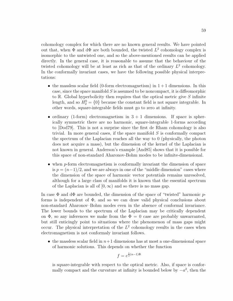
59

cohomology complex for which there are no known general results. We have pointedout that, when Φ and dΦ are both bounded, the twisted L2 cohomology complex isisomorphic to the untwisted one, and so the above-mentioned results can be applieddirectly. In the general case, it is reasonable to assume that the behaviour of thetwisted cohomology will be at least as rich as that of the ordinary L2 cohomology.In the conformally invariant cases, we have the following possible physical interpre-tations:

• the massless scalar field (0-form electromagnetism) in 1 + 1 dimensions. In thiscase, since the space manifold S is assumed to be noncompact, it is diffeomorphicto R. Global hyperbolicity then requires that the optical metric give S infinitelength, and so H0

2 = 0 because the constant field is not square integrable. Inother words, square-integrable fields must go to zero at infinity.

• ordinary (1-form) electromagnetism in 3 + 1 dimensions. If space is spher-ically symmetric there are no harmonic, square-integrable 1-forms accordingto [Dod79]. This is not a surprise since the first de Rham cohomology is alsotrivial. In more general cases, if the space manifold S is conformally compactthe spectrum of the Laplacian reaches all the way to 0 (physically, the photondoes not acquire a mass), but the dimension of the kernel of the Laplacian isnot known in general. Anderson’s example [And85] shows that it is possible forthis space of non-standard Aharonov-Bohm modes to be infinite-dimensional.

• when p-form electromagnetism is conformally invariant the dimension of spaceis p = (n−1)/2, and we are always in one of the “middle dimension” cases wherethe dimension of the space of harmonic vector potentials remains unresolved,although for a large class of manifolds it is known that the essential spectrumof the Laplacian is all of [0,∞) and so there is no mass gap.

In case Φ and dΦ are bounded, the dimension of the space of “twisted” harmonic p-forms is independent of Φ, and so we can draw valid physical conclusions aboutnon-standard Aharonov–Bohm modes even in the absence of conformal invariance.The lower bounds to the spectrum of the Laplacian may be critically dependenton Φ, so any inferences we make from the Φ = 0 case are probably unwarranted,but still enticingly point to situations where the phenomenon of mass gaps mightoccur. The physical interpretation of the L2 cohomology results in the cases whenelectromagnetism is not conformaly invariant follows.

• the massless scalar field in n+1 dimensions has at most a one-dimensional spaceof harmonic solutions. This depends on whether the function

f = e12(n−1)Φ

is square-integrable with respect to the optical metric. Also, if space is confor-mally compact and the curvature at infinity is bounded below by −a2, then the

60

essential spectrum of the Laplacian is [a2(n − 1),∞). This means that, if thedimension of space is n > 1, the free massless scalar field can have a mass gapin the Φ = 0 case.

• ordinary electromagnetism in 2+1 dimensions can have an infinite-dimensionalspace of harmonic vector potentials even in the rotationally symmetric case,including when the optical metric on space is that of the hyperbolic plane. Inaddition, if space is conformally compact the Φ = 0 mass gap is a2/4, where −a2

is the lower bound to the curvature at infinity. When the optical metric on spaceis conformally compact and of dimension 4+1 or higher, the space of harmonicvector potentials is isomorphic to the first cohomology of M relative to itsboundary, and so there are no non-standard Aharonov–Bohm modes. Whenthe curvature at infinity is bounded below by −a2, the essential spectrum ofthe ordinary Laplacian is [a2(n − 3),∞) if n ≥ 3, signaling the possibility oftopological mass gaps in 4 + 1 dimensions or higher, at least when Φ = 0.

• for p-form electromagnetism, there is an infinite-dimensional space of harmonicvector potentials if space is a 2p-dimensional and rotationally symmetric orconformally compact. In the latter case, there is a Φ = 0 mass gap of a2/4.If |n−2p| > 1 there are no non-standard Aharonov-Bohm modes, but the Φ = 0mass gap is zero only if n = 2p± 1.

61

Part II

Quantum electromagnetism

62

The apparent truism that a quantum mechanical theory needs to be cast in clas-sical language in order to correlate its predictions with our experience, a point thatNiels Bohr made into a cornerstone of his philosophy of quantum mechanics, has prac-tical consequences for the development of quantum descriptions of physical systems.This is because a physical system will be described operationally or geometrically ininevitably classical terms, and this information needs to be fashioned into a quantumtheory whose predictions need to be, again, reexpressed in classical terms. In addi-tion, the process of constructing a classical theory from operational or geometric datais so well-understood that it is convenient to construct the quantum theory by firstconstructing a classical theory from the data and then ‘quantizing’ it.

Quantization is a catch-all term for any process taking as input a classical me-chanical system, and producing as output a quantum mechanical system reducing tothe original classical system in an appropriate limit. Quantization would ideally bealgorithmic or functorial, but it turns out to be neither, although formulating quan-tization in algebraic language seems to bring it closest to the goal of functoriality.

In algebraic terms, a classical mechanical system is defined by specifying a Poissonalgebra of observables, while any associative algebra can play the role of algebraof observables for a quantum system. The Dirac quantization prescription [Dir57,Chapter IV] ‘promotes’ the commuting classical observables to operators satisfyingthe Heisenberg commutation relations

[f , g] = i~f, g,where f, g is the Poisson bracket of the classical observables f and g, [f , g] is thecommutator of their quantum counterparts, and Planck’s constant ~ measures thedeparture from classical behaviour (where observables commute). It is not hard toconvince oneself that, because the algebra of quantum observables is nonabelian, theoperation f 7→ f cannot be an algebra homomorphism. That is, f g 6= f g in general.Physicists call this fact ‘operator ordering ambiguities’.

An operator algebra of quantum observables realizing the canonical commutationrelations achieves quantization in a kinematical sense, but the physical and dynam-ical content of the theory comes about by means of a specific representation of thequantum observables as an algebra of (unbounded) linear operators on a Hilbertspace of quantum states. Each representation is associated to a choice of ‘vacuumexpectation’ on the algebra of observables and it is known that, for systems withinfinitely many degrees of freedom, different states may lead to unitarily inequivalentrepresentations. The choice of representation can be narrowed down by the need torecover an appropriate classical limit, and by requiring that physical symmetries beimplemented unitarily.

The classical limit is encoded in the correspondence principle, by which we meanthe following. The Poisson algebra of classical observables consists of smooth func-tions on a symplectic manifold (phase space) playing the role of state space for theclassical theory. The correspondence principle requires that, for any phase space

63

point x ∈ P and any observable f , there should be a quantum state |x〉 such that theexpected value of f in the state |x〉 equals the classical value f(x), if not exactly, atleast in the limit ~ → 0. That is,

〈x| f |x〉 = f(x) +O(~).

There is one last requirement that a sensible quantization must satisfy, and thatis that physical symmetries be represented by unitary operators on the Hilbert spaceof quantum states of the system.

In the case where the classical phase space is a vector space, the linear observablescan be identified with the points of the phase space itself, and so the Heisenberg com-mutation relations can be implemented on the phase space. In Chapter 5 we developthe quantization of an abstract linear system and develop the concept of a quasiop-erator on Fock space, and in Chapter 6 we apply this to Maxwell’s equations for theelectromagnetic field and express the dynamics of the quantized electromagnetic fieldin terms of Wilson loops quasioperators.

The work most closely akin to ours is that of Dimock [Dim92]. Like us, Dimockconstructs a C∗-algebra of observables for the electromagnetic field, but he does notexhibit any states or Hilbert-space representations. He notes in passing that “in anycase such [Hilbert-space] representations exist, say by a Fock space construction”. Wediscuss below some ways in which a Fock space representations may fail to exist.

Because Dimock describes the classical theory in the covariant canonical formal-ism, he is forced to focus on “the algebraic structure of the theory, not in the spec-ification of particular states”. In our terms, Dimock quantizes the electromagneticfield as a ‘general boson field’. He also constructs a classical Poisson bracket, and hisquantization procedure is equivalent to our general linear quantization. Dimock doesshow that different Hilbert-space representations lead to ∗-isomorphic C∗-algebras ofobservables. This form of equivalence, however, obviates the possible physical conse-quences of unitary inequivalence of Hilbert-space representations, and for this reasonDimock’s paper suffers from what Earman and coauthors critically term “algebraicimperialism” in [AER02].

Dimock does not show that the classical canonical transformations associatedto changes in the choice of Cauchy surface are implemented unitarily on the C∗-algebras of quantum observables, because that is simply not true. In fact, Torre andVaradarajan [TV99] show that, even in the case of free scalar fields on a flat spacetimeof dimension higher than two, there is no unitary transformation between the Fockrepresentations associated to arbitrary initial and final Cauchy surfaces. They pointout that unitary implementability is easily obtained if the Cauchy surfaces are relatedby a spacetime isometry, though. They also mention related results of Helfer (nounitary implementation of the S-matrix if the ‘in’ and ‘out’ states are Hadamardstates) [Hel96], and of van Hove (only a small subgroup of the classical canonicaltransformations is unitarily implementable) [VH51].

64

Another paper addressing specifically the quantization of the electromagnetic fieldis the one by Corichi [Cor98]. Corichi stresses that Fock quantization depends cru-cially on the linear structure of phase space, and characterizes the Fock quantizationprocedure as “completely elementary”.

Here we perform Fock quantization of Maxwell’s equations on a static, globallyhyperbolic spacetime with a trivial R bundle on it. Presumably this can be extendedto stationary spacetimes, but not beyond that because of the need for a nontrivialgroup of isometries. The treatment of nontrivial or U(1) bundles should require onlystraightforward modifications, but one of the lessons of our work is that sometimesthere are surprises in store even for topics as well-understood as electromagnetism.

In chapter 6, because of the appearance of negative powers of the Laplacian ∆(or the twisted Laplacian Lp in the general case) in the process, we will be forcedto restrict Fock quantization to the space Po of oscillating modes of the electromag-netic field. Also, for mathematical convenience one often assumes that ∆ ≥ ǫ > 0for some ǫ, which is true when space is compact but not necessarily when it is non-compact. However, we do not do this as one cannot exclude the possibility that thespectrum of Lp or ∆ reach all the way to 0 because that is the case in physicallyinteresting situations such as Minkowski space.

65

Chapter 5

Coherent-state quantization oflinear systems

In this chapter we present a rigorous framework for quantization of linear dynamicsbased on the ideas of Irving Segal.

Segal pioneered the idea of of formalizing quantum mechanics in terms of algebrasof observables, making Hilbert spaces play the subordinate role of supporting linearrepresentations of them. These Hilbert spaces can, in fact, be constructed from theabstract algebra of observables by means of the Gel’fand–Naımark–Segal constructionusing a single state or, in physics parlance, vacuum expectation.

Implicit in the work of Segal is a concept of general boson field associated to anylinear phase space, which formalizes the Heisenberg commutation relations amongfield operators in terms of exponentiated field operators, using the so-called Weylrelations. This has the advantage of avoiding the technicalities of unbounded opera-tors. In addition, physical symmetries are readily implemented as automorphisms ofthe Weyl algebra.

Segal introduced the related concept of free boson field , which can be constructedfrom a phase space equipped with a compatible complex structure. Segal’s free bosonfield axiomatizes the properties of the usual of Fock space, and the axiomatic approachmakes it transparent that the Fock, Schrodinger and Bargmann–Segal representationsof linear quantum fields are all unitarily equivalent. Within this framework, Segalalso studied the problem of representing time evolution unitarily on Fock space, andthe stability of the generator of unitary time evolution, namely whether the quantumHamiltonian is bounded below.

Here we put together both ideas, and the result is a new construction of the freeboson field based on coherent states. In this construction we not only associate toeach linear functional on phase space a field operator but, given a choice of vacuumstate, we can associate to each point in phase space a coherent state. The collectionof all coherent states indexed by points of phase space spans the Hilbert space ofquantum states of the theory, and the result is what Segal called the general boson

66

field. The free boson field, which as we have mentioned is unitarily equivalent to theFock representation, is obtained by means of a GNS state with Gaussian statistics.

We find that the mathematical process of quantization can be understood withreference to three physical guiding principles: the canonical commutation relations,the correspondence principle, and the unitary implementation of physical symmetries.

We proceed as follows: we first construct the Weyl algebra of observables associ-ated to a linear phase space, and then choose a compatible complex structure on thePhase space, which amounts to selecting a vacuum expectation on the Weyl algebra,with the help of the correspondence principle and the requirement that time evolutionbe unitarily and stably implemented.

Coherent states are most useful because many classical equations hold exactlybetween expectation values on coherent states. Thus, by using coherent states, ourquantization procedure never loses sight of the correspondence principle. In addition,the vacuum expectation value acts as a generating function of the matrix elements offield operators between coherent states, not only for ordinary field operators but alsofor their Wick powers (called normal-ordered operators in physics). As an unexpectedbonus, using matrix elements between coherent states one can define normal-orderedWilson loops as quasioperators without the need for regularization.

Segal’s treatment of the free boson field is presented in [BSZ92]. A comprehensivephysical treatment of the coherent states of the electromagnetic field can be foundin [MW95, Chapter 11].

67

5.1 The general boson field

The development that follows may seem idiosyncratic to those familiar with thetraditional quantization methods and the notations used in physics. In particular,we insist on distinguishing the phase space P from its dual P∗. There are somegood reasons for this. At the present stage of development of mathematical physics,the most compelling reason for studying the quantization of a linear systems is as aspringboard for quantization of nonlinear systems, or as a testing ground for ideassuggested by the study of nonlinear systems. Our approach is motivated by the factthat the ordinary quantization of linear systems makes use of several identificationsthat can only be made for a linear system. Adopting the view that a classical me-chanical system is characterized by its Poisson algebra of observables, the cotangentspace at each point of phase space acquires a symplectic structure. When the phasespace P is linear, the following identifications can be made: the dual P∗ can be iden-tified with the linear observables, and the restriction of the Poisson bracket to P∗ isa symplectic structure. Also, the cotangent spaces to each point of phase space arecanonically isomorphic to each other and to P∗, and the globally-defined symplecticstructure on P∗ makes P isomorphic to P∗ and also endows it with a symplecticstructure. All of these identifications, and even the possibility of considering itself Pto be a symplectic vector space, are accidents of linearity. Accordingly, we will avoidmaking use of these features as much as possible. Every time we are forced to makeuse of one of these identifications, it will be a sign that the procedure cannot bereadily generalized to nonlinear situations.

5.1.1 Linear phase spaces

We start by formalizing the notion of linear phase space, which is the necessaryclassical input of our quantization procedure.

Definition 3 (linear phase space). A linear phase space is a reflexive real topo-logical vector space P whose dual P∗ is a symplectic vector space. That is, P∗ isa topological vector space equipped with a symplectic structure: a continuous, skew-symmetric bilinear form ω which is weakly nondegenerate in the sense that the dualitymap ∗:P∗ → P given by

ω(f, g) = f(g∗) for all f, g ∈ P∗

is injective.

Note. Without the assumption that P is reflexive, the duality map would be ∗:P∗ →P∗∗. This would have a bearing on the definition of the Hilbert space of quantumstates below.

A finite-dimensional vector space has a unique Hausdorff topology, and any infinite-dimensional vector space can be topologized algebraically [BSZ92, §1.2]; in either case

68

the continuity of ω is vacuously true. In general, the dual P∗ of a topological vectorspace is itself naturally a topological vector space, with the weak-∗ topology mak-ing every element of P a continuous linear functional on P∗. If P has a normedtopology, P∗ can also be given the (normed) strong operator topology. In eithercase, P ⊆ P∗∗ is a continuous inclusion.

The right notion of automorphism of a linear phase space is the following. Recallthat, if T :P → P is linear, there is a unique linear map T ∗:P∗ → P∗ called its dualsuch that

(T ∗f)(x) = f(Tx) for all x ∈ P, f ∈ P∗.

Definition 4 (automorphism of a linear phase space). An automorphism ofthe linear phase space P is a continuous invertible linear map T :P → P whose dualmap T ∗:P∗ → P∗ preserves the symplectic structure on P∗.

The space of states of a classical system is its physical phase space P , namely thespace of gauge equivalence classes of solutions of its equations of motion. Similarly,its algebra of observables consists of smooth gauge-invariant functions of solutions tothe equations of motion, C∞(P ). The classical algebra of observables is naturallya Poisson algebra, but the physical phase space P need not be a Poisson manifold,let alone a symplectic vector space. For instance, in Yang–Mills theory P is somesort of ‘singular infinite-dimensional variety’, a concept without a precise definition.Continuous non-gauge symmetries of the physical system are are represented by auto-morphisms of the Poisson algebra of observables generated through Poisson bracketswith appropriate observables: the conserved quantities associated to the symmetriesvia Noether’s theorem.

Suppose, then, that not only C∞(P ) is a Poisson algebra with Poisson bracket , but that P is a manifold. The Poisson bracket defines a bivector ω: Ω2(P ) → R givenby

ω(df, dg) = f, g for all f, g ∈ C∞(P).

If ω is non-degenerate at x ∈ P , the space T ∗xP becomes a symplectic vector space.

In physical terms, x is a field configuration and T ∗xP is the space of linear observables

in the vicinity of this field configuration. This is the only symplectic vector spacethat can be constructed in a natural way from the phase space P , and Definition 3applies with P = TxP and ω = ωx. In these favourable cases, symmetries of fieldconfigurations x ∈ P are Poisson maps leaving x fixed, which induce linear symplectictransformations of T ∗

xP .Identifying all the T ∗

xP amounts to choosing a trivialization of T ∗P , and this isnatural only if P is a linear space admitting a canonical flat connection. In that case,each of the T ∗

xP is canonically isomorphic to P ∗ itself. When the equations of motionare linear, one can take P = P in Definition 3, and restrict one’s attention to linearobservables and symmetry transformations.

69

5.1.2 Quantizing a linear phase space

Linear quantization is a process “promoting” each x ∈ P to a unit vector |x〉 in asuitable Hilbert space K, and each f ∈ P∗ to a self-adjoint operator f on K, in sucha way that the Heisenberg commutation relations

[f , g] = iω(f, g)1K for all f, g ∈ P∗ (5.1)

hold. Equation 5.1 is a restricted form of the Dirac quantization prescription, sinceit is applied only to linear observables on P, and not to arbitrary ones as it wasoriginally formulated. In addition, the correspondence principle is required to holdin the form

〈x| f |x〉 = f(x) for all x ∈ P, f ∈ P∗, (5.2)

without allowing for corrections of order ~. Finally, one would hope to representevery physical symmetry T :P → P as a unitary operator UT :K → K in such away that USUT = UST for all symplectic maps S, T :P → P. As we shall see, ingeneral this is only possible for a subgroup of linear symplectic transformations of Pand, in fact, choosing a small subgroup of physical symmetries that must be unitarilyimplemented can be enough to determine K, sometimes uniquely. Time evolution isalways required to be a physical symmetry and, in this sense, the dynamics determinethe quantization.

Canonical commutation relations

The Heisenberg relations cannot be implemented on an algebra of bounded op-erators [Rud91, §13.6], and so Equation 5.1 must be understood as holding on the(hopefully) dense domain of [f , g] in K. This is only the first of a long list of nuisancesthat arise from necessarily dealing with unbounded operators, but all the same weencode it as a definition.

Definition 5 (Heisenberg system). A Heisenberg system on a symplectic vectorspace (P∗, ω) is a real-linear map Φ: f 7→ Φ(f) from P∗ to the self-adjoint operatorson some complex Hilbert space K, satisfying the Heisenberg commutation relations

[Φ(f),Φ(g)] = iω(f, g)1K. for all f, g ∈ P∗

as an operator equation holding on the common domain of Φ(f)Φ(g) and Φ(f)Φ(g),which is assumed to be dense. The operator Φ(f) is called the Heisenberg operatorassociated to f ∈ P∗.

In other words, linear quantization is partially achieved by constructing a Heisen-berg system on the space of linear observables (P∗, ω). However, there are lots ofHeisenberg systems that have nothing to do with physics, examples of which canbe found in [MR80, BSZ92], so for honest quantum physics one needs to impose

70

some additional regularity on the Heisenberg systems. This is achieved in an some-what circuitous way by considering the unitary groups supposedly generated by theHeisenberg operators. Heuristically, if Φ(f) is a Heisenberg operator on K, the op-erator W (f) = e−iΦ(f) is unitary and, since [Φ(f),Φ(g)] commutes with both Φ(f)and Φ(g), the Baker–Campbell–Hausdorff formula applies, giving

e−iΦ(f)e−iΦ(g) = e−iΦ(f+g)e−12[Φ(f),Φ(g)].

We take this heuristic calculation as the motivation of our next definition.

Definition 6 (Weyl algebra). The Weyl algebra on a symplectic vector spacespace (P∗, ω), is the complex ∗-algebra W(P∗, ω) generated by the set W(P∗) =W(f)f∈P∗ , of Weyl operators, modulo the unitarity relations

W(f)∗ = W(−f) for all f ∈ P∗

and the Weyl relations

W(f)W(g) = eω(f,g)/2iW(f + g) for all f, g ∈ P∗.

Note. Because the Weyl relations reduce products of Weyl operators to single Weyloperators, the Weyl algebra W(P, ω) coincides with the linear span of W(P). Infact, W(P) is a basis of W(P, ω).

Heuristically, because of the Baker–Campbell–Hausdorff formula above, one wouldexpect that a Heisenberg system can be constructed from a representation of the Weylalgebra as an algebra of operators on a suitable Hilbert space. Such a representationis called a Weyl system. We will consistently use the fonts W and W to distinguishthe abstract Weyl algebra W(P, ω), and its generators W(x), from Weyl systems Wassociated to concrete Hilbert-space representations of the Weyl algebra.

Definition 7 (Weyl system). A Weyl system on the symplectic vector space (P∗, ω)is a continuous mapping W :P∗ → U(K), where U(K) is the group of unitary opera-tors on the complex Hilbert space K with the strong operator topology, and W satisfiesthe Weyl relations

W (f)W (g) = eω(f,g)/2iW (f + g) for all f, g ∈ P∗.

Note. Since a Weyl system is required to be continuous in the strong operator topol-ogy on U(K), the map t 7→ W (tf) is a strongly-continuous one-parameter subgroupof U(K). By Stone’s theorem [RS80, §VIII.4], this one-parameter subgroup has aself-adjoint generator Φ(f) such that W (f) = e−iΦ(f).

Lemma 17. IfW :P∗ → U(K) is a Weyl system on the symplectic vector space (P∗, ω)then Φ:P∗ → L(K) is a Heisenberg system on (Φ∗, ω). In addition, for all x, y ∈ P,the operator Φ(f) + iΦ(g) is closed and Φ(f + g) is the closure of Φ(f) + Φ(g).

71

Sketch of proof. Differentiating the Weyl relation

W (tf)W (tg) = et2ω(f,g)/2iW (t(f + g))

twice and setting t = 0, one obtains that f 7→ Φ(f) is additive and satisfies theHeisenberg commutation relations

[Φ(f),Φ(g)] = iω(f, g)1K.

The proof of the closure properties of the Heisenberg operators is in [BSZ92, §1.2].

At this point, a theorem of von Neumann [MR80, §VIII.5] guarantees that all Weylsystems on a finite-dimensional phase space are unitarily equivalent. At any rate, wesee that Weyl systems are the right formalization of Equation (5.1), the Heisenbergcommutation relations. The following lemma shows one reason why it is convenientto insist that physical symmetries be represented by linear symplectic maps on P.

Lemma 18. Suppose that γ:W(P∗, ω) → W(P∗, ω) is a ∗-algebra endomorphismsuch that

for every f ∈ P∗, γ(W(f)) = W(g) for some g ∈ P∗,

and suppose furthermore that the map T ∗: (P∗, ω) → (P∗, ω) given by T ∗f = g iscontinuous. Then, T ∗ is in fact linear and preserves the symplectic structure ω. If, inaddition, γ is an automorphism, then T ∗ is invertible, that is, T is an automorphismof the linear phase space P.

What this means is that the formalization of quantization using Weyl systems isbest suited to the case when physical symmetries—in particular, time evolution—arelinear.

Proof. Assuming γ is a ∗-algebra endomorphism,

γ(W(f))γ(W(h)) = γ(W(f)W(h))

so, applying the definition of T ∗ on the left-hand side and the Weyl relations on theright-hand side,

W(T ∗f)W(T ∗h) = γ(eω(f,h)/2iW(f + h)).

Now, the Weyl relations on the left-hand side and the properties of γ on the right-handside imply

eω(T ∗f,T ∗h)/2iW(T ∗f + T ∗h) = eω(f,h)/2iW(T ∗(f + h)).

Since all the W(f)f∈P∗ are linearly independent by construction, it follows that T ∗

is additive and preserves ω. Finally, continuous additive functions are linear.

The converse of this result is also true.

72

Lemma 19. If T :P → P is an automorphism of the linear phase space P, then thereexists a unique ∗-algebra automorphism γ(T ):W(P∗, ω) → W(P∗, ω) determined by

γ(T ):W(T ∗f) 7→ W(f) for all f ∈ P∗

and such that γ(ST ) = γ(S)γ(T ).

In other words, γ is the unique representation of the group of symplectic auto-morphisms of (P∗, ω) as ∗-algebra automorphisms of W(P∗, ω) mapping the set ofgenerators W(f): f ∈ P∗ to itself. This result is related to [BSZ92, Corollary 5.1.1].

Proof. Applying γ(T ) to both sides of the Weyl relation

W (T ∗f)W (T ∗g) = eω(T ∗f,T ∗g)/2iW (T ∗(f + g)) for all f, g ∈ P∗

we obtain

W (f)W (g) = eω(T ∗f,T ∗g)/2iW (f + g) for all f, g ∈ P∗,

so γ(T ) is an automorphism because T ∗ is symplectic. Also, if S, T :P → P are twoautomorphisms of P,

γ(S)γ(T )W((ST )∗f) = γ(S)γ(T )W(T ∗S∗f)

= γ(S)W(S∗f)

= W(f)

= γ(ST )W((ST )∗f)

for all f ∈ P∗.

Definition 8 (general boson field). If (P∗, ω) is a symplectic vector space, thegeneral boson field over it is the pair (W, γ) where W: f 7→ W(f) is the map from P∗

to W(P∗, ω), and γ is the representation of automorphisms of P by ∗-automorphismsof W(P∗, ω) mentioned in Lemma 19.

Note. This definition is implicit in [BSZ92, §5.3].

In sum, given any linear phase space space P with dual (P∗, ω) one can constructthe associated Weyl algebra W(P∗, ω), which supports a representation γ of theautomorphisms of P as ∗-algebra automorphisms of W(P∗, ω). In addition, anyWeyl system on (P∗, ω), that is, any strongly continuous representation of W(P∗, ω)as unitary operators on a complex Hilbert space K provides a realization of theHeisenberg commutation relations. This is the general boson field on P.

73

Correspondence principle

The general boson field realizes the canonical commutation relations and the phys-ical symmetries of a linear system, but it does not provide a complete quantizationof a linear phase space, as there are a few lingering issues. The first is how to actu-ally construct Weyl systems. The second is whether the correspondence principle issatisfied. The third is whether physical symmetries are implemented unitarily on thesupporting Hilbert space of the Weyl system. It turns out that all three are related.In this section we will first use the Gel’fand–Naımark–Segal construction to produceWeyl systems, and then use the correspondence principle and unitary implementabil-ity of physical symmetries to select the Weyl systems that produce physically sensiblequantizations.

The following example constructs the so-called Schrodinger representation of theHeisenberg commutation relations in one dimension.

Example. We choose units such that ~ = 1. Let K = L2(R) and, for each f = (a, k) ∈R2, define

[W (f)ψ](x) = e−ik(x−a/2)ψ(x− a) for all ψ ∈ K,

which clearly makes W (f) a unitary operator on K. Also,

W (f)W (f ′) = e(ka′−k′a)/2iW (f + f ′)

so W is a Weyl system on the linear phase space P = R2 with

P∗ = f = (a, k) ∈ R2 and ω(f, f ′) = ka′ − k′a.

The Heisenberg operators are given by

Φ(f)ψ(x) = (kx− ia∂x)ψ(x).

This Heisenberg system is called the Schrodinger representation.Given that Φ is linear, it might seem odd that the momentum coordinate k appears

as the coefficient of the operator of multiplication by x, which we would usually withthe position operator. In addition, the symplectic structure ω(f, f ′) = ka′−k′a seemsbackwards. We now proceed to explain these features of the representation.

The configuration space is R with coordinate function q: R → R satisfying q(x) =x, and the phase space is P = R2 with coordinate functions q, p: R2 → R (p beingthe momentum coordinate function). Then, dp and dq are a basis of P∗, and (a, k)are coordinates on P∗ with respect to that basis. That is, we identify f = (a, k)with f = adp + kdq. This is the correct pairing despite what our intuition mightsuggest, namely pairing a with q since they both refer to the same quantity (position),because ps+ qk has homogeneous units of action while qs+ pk is not a homogeneousquantity. We are, in fact, omitting factors of Planck’s constant ~ as we have chosen‘natural units’ in which ~ = 1 according to custom.

74

The linear observables q (position) and p (momentum) on P have Poisson bracket

q, p = 1.

Accordingly, the dual P∗ is generated by dq, dp with symplectic structure

ω(dq, dp) = q, p = 1.

In other words,P∗ = f = kdq + adp: a, k ∈ R

and the symplectic structure on P∗ is

ω(f, f ′) = ω(kdq + adp, k′dq + a′dp) = ka′ − k′a.

So, the apparently contradictory

q, p = 1 and ω((a, k), (a′, k′)) = ka′ − k′a

are entirely consistent. Then, we have

Φ(dq)φ(x) = xφ(x) and Φ(dp)φ(x) = −i∂xφ(x)

as expected, and if f = (a, k),

Φ(f) = aΦ(dp) + kΦ(dq).

It is clear how this representation can be extended to any finite number of di-mensions, and by the theorem of von Neumann alluded to after Lemma (17), theserepresentations are unique up to unitary equivalence. For the infinite-dimensionalcase relevant to field theories, though, one needs to use the Gel’fand–Naımark–Segalconstruction, which is based on the concept of a state and leads to possibly unitarilyinequivalent representations.

Definition 9 (GNS state). A state on a ∗-algebra A is a linear functional

〈 〉:A→ C

which is nonnegative〈a∗a〉 ≥ 0 for all a ∈ A,

and normalized〈1〉 = 1.

75

Note. The usage here is completely analogous to that for linear functionals on vectorspaces. A purely algebraic definition of linear functional on a vector space requiresthat it be defined everywhere, but when a topology is introduced one finds it usefulto consider discontinuous, densely-defined linear functionals. In the same vein, aslong as the algebra A is not assumed to have a topology, one must require thatstates be defined on all of A. However, if A has a topology making addition andmultiplication continuous, then one can talk about continuous or bounded states,and also about discontinuous, densely-defined states. At this point, W(P∗, ω) doesnot have a topology defined on it so states on it should be defined everywhere. On theother hand, the Weyl system W (P∗, ω) on K is given the strong operator topology,and so densely-defined states make sense on it. In fact, we will use a state on W(P∗, ω)to construct K, and it is not guaranteed that the state will be everywhere defined onit.

A state on W(P∗, ω) defines a nonnegative-definite sesquilinear form 〈 | 〉on W(P∗, ω) by means of

〈W | W ′〉: = 〈W∗W ′〉 for all W,W ′ ∈ W(P∗, ω).

Note that, since 〈W(f) | W(g)〉 = 〈W(−f)W(g)〉,

〈W(f) | W(g)〉 = eiω(f,g)/2〈W(g − f)〉 for all f, g ∈ P∗. (5.3)

The associated nonnegative quadratic form

|W|2 = 〈W|W〉

is finite on all of W(P, ω), since

|W(f)| = 1 for all f ∈ P∗.

However, it can only be guaranteed to be a seminorm, because it is possible that 〈 〉has a kernel. However, this kernel is necessarily invariant under multiplication byelements of W(P∗, ω). Indeed, that |W| = 0 is equivalent to 〈W(f) | W〉 = 0 forall f ∈ P∗. But then

〈W(f) | W(g)W〉 = 〈eω(f,g)/2iW(f − g) | W〉 for all f ∈ P∗

implies that |W(g)W| = 0 for all g ∈ P∗.By the standard procedure—namely, taking the quotient of W(P∗, ω) by the null

subspace of | | and completing the result with respect to | | (which is a norm afterquotienting by the null subspace)—one can construct a complex Hilbert space K withinner product 〈 | 〉. The invariance of the null space of | | under the multiplicativeaction of W(P∗, ω) implies that W(P∗, ω) acts on K.

This is a version of the Gel’fand–Naımark–Segal construction. We now show thatwe can give a description of K in terms of the phase space P. For this, we draw thefollowing definition from [BSZ92, §5.3].

76

Definition 10 (characteristic functional). If 〈 〉 is a state on the Weyl alge-bra W(P∗, ω), its characteristic functional µ:P∗ → C is given by

µ(f): = 〈W(f)〉 for all f ∈ P∗. (5.4)

We say the state 〈 〉 is regular if, for every f ∈ P∗, the function

t 7→ µ(tf) (t ∈ R)

is twice differentiable at t = 0.

Note. We will find it convenient to introduce the following notation:

∂fµ(g) =∂

∂t

∣∣∣∣t=0

µ(g + tf).

Theorem 20. Let (P∗, ω) be a symplectic vector space. Then, given a regular state 〈 〉on W(P∗, ω) with characteristic function µ, there is an x ∈ P such that

i∂fµ(0) = f(x) for all f ∈ P∗.

Then, the collection of formal symbols Ψ = |x+ f ∗〉 : f ∈ P∗ generates a complexvector space with the following properties:

1. the sesquilinear form

〈x+ f ∗ | x+ g∗〉 = eω(g,f)/2iµ(g − f) (5.5)

makes the span of Ψ into a complex pre-Hilbert space whose Hilbert space com-pletion is denoted K

2. there is a Weyl system W :P∗ → U(K) on (P∗, ω), given by

W (f) |x+ g∗〉 = eω(f,g)/2i |x+ f ∗ + g∗〉 for all f, g ∈ P∗ (5.6)

3. the unit vector |x〉 ∈ K is a cyclic vector of the Weyl system W (P∗, ω)

4. the associated Heisenberg system Φ:P∗ → L(K) satisfies

〈x+ g∗|Φ(f) |x+ g∗〉 = f(x+ g∗) for all f, g ∈ P∗.

77

P

•x

??x+f∗

Figure 5.1: schematic representation of the relative coherent states as an affine sub-space of phase space

The last property states that the Heisenberg system obtained from the regularstate 〈 〉 satisfies the correspondence principle. Namely, the expected value of thequantum observable Φ(g) in the quantum state |x+ f ∗〉 equals the value of the clas-sical observable g ∈ P∗ in the classical state x+ f ∗ ∈ P.

Because we have not assumed that the symplectic structure ω makes the dualitymap ∗:P∗ → P onto, it is possible that x 6= f ∗ for any f ∈ P∗, in which case thecollection of indices x+ f ∗: f ∈ P∗ is an affine subspace of P. In other words, if ωis only weakly and not strongly nondegenerate, not every classical state in P has acounterpart in K.

The physical interpretation of the vector x ∈ P is that of a classical ‘background’field configuration, since 〈x|Φ(f) |x〉 = f(x) for every classical linear observable f ∈P∗. Clearly any other density operator in K can be used to define a state leadingto a unitarily equivalent Weyl system, possibly with a different background fieldconfiguration. If x is not of the form g∗ for any g ∈ P∗, it will actually be impossibleto eliminate the background altogether by a unitary change of representation.

Finally, the fact that the span of Ψ is dense in the Hilbert space K will be used con-sistently in the sequel to characterize densely defined linear operators and sesquilinearforms on K.

Proof. This proof has a curious way of pulling itself up by its own bootstraps: themain conceptual difficulty is that, in order to show that f 7→ i∂fµ(0) is a continuouslinear functional on P∗ one needs to have the Weyl system W in place. We proceedby constructing Ψ and K before the names |x+ f ∗〉 are available, and then renamingthe vectors after x is shown to have the advertised properties.

We will temporarily denote by ψf ∈ K the image of W(f) under the GNS con-struction described immediately before Definition 10. We denote Ψ = ψf : f ∈ P∗.It follows immediately from Equation (5.3) that

〈ψf | ψg〉 = eiω(f,g)/2µ(g − f) for all f, g ∈ P∗. (5.7)

The span of Ψ, which consists of unit vectors, is dense in K with respect to this innerproduct. Recall also that, in the lead-up to Definition 10, we showed that the action

78

of W(P∗, ω) on itself by left multiplication projects to K by virtue of the invarianceof the null space of 〈 | 〉. This action, namely the Weyl relations, passes to thequotient as

W (f)ψg = eω(f,g)/2iψf+g for all f, g ∈ P∗. (5.8)

We are now ready to construct a Weyl system W :P∗ → U(K). The follow-ing lemma shows that the Hilbert space K automatically supports a Weyl sistemon W(P∗, ω).

Lemma 21. Suppose that a regular state 〈 〉 is given on the Weyl algebra W(P, ω)and the GNS construction is performed resulting in the Hilbert space K, as just de-scribed. Then, Equation (5.8) defines a map W :P∗ → U(K) which is a Weyl systemon (P∗, ω). In addition, the unit vector ψ0 ∈ K is a cyclic vector of the Weyl sys-tem W :P∗ → U(K).

Proof. First, we need to show that W (f) ∈ U(K) for all f ∈ P∗. Indeed, observethat W (f) maps Ψ to itself and that, for all f, g, h ∈ P∗,

〈W (f)ψg |W (f)ψh〉 = eω(f,h−g)/2i〈ψf+g | ψf+h〉= eω(f,h−g)/2ieiω(f+g,f+h)/2µ(h− g)

= eiω(g,h)/2µ(h− g) = 〈ψg | ψh〉This implies that W (f) is an invertible isometry on the span of Ψ. Then, by densityof the span of Ψ in K and linearity, it follows that W (f) is unitary on K.

Now, we need to show that, for all f, g, h ∈ P∗,

W (f)W (g)ψh = eω(f,g)/2iW (f + g)ψh.

The left-hand side is equal to

W (f)eω(g,h)/2iψg+h = eω(g,h)/2i eω(f,g+h)/2i ψf+g+h,

and the right-hand side is equal to

eω(f,g)/2iW (f + g)ψh = eω(f,g)/2i eω(f+g,h)/2i ψf+g+h.

To show strong continuity of the Weyl system W we need to show that, if fn → fin P∗, then W (fn) → W (f) in the strong operator topology on U(K). To this end,we consider

[W (f) −W (g)]ψh = eω(f,h)/2iψf+h − eω(g,h)/2iψg+h.

Then,‖[W (f) −W (g)]ψh‖2 = 2Re[1 − eiω(f−g,h)+iω(f,g)/2µ(g − f)],

which indeed vanishes as f − g → 0 because of the continuity of ω and µ and theantisymmetry of ω.

Finally, the unit vector ψ0 ∈ K is a cyclic vector of the Weyl system W :P∗ →U(K) because W (f)ψ0 = ψf for all f ∈ P∗, and the collection of all ψf is densein K.

79

We now study the Heisenberg system associated to the Weyl system defined inLemma 21.

Lemma 22. In the hypotheses of Lemma 21, 〈ψg | Φ(f)ψg〉 and ‖Φ(f)ψg‖ are bothfinite for all f, g ∈ P∗. Moreover,

〈ψg | Φ(f)ψg〉 = ω(f, g) + 〈ψ0 | Φ(f)ψ0〉and

‖Φ(f)ψg‖2 − ‖Φ(f)ψ0‖2 = 〈ψg | Φ(f)ψg〉2 − 〈ψ0 | Φ(f)ψ0〉2.Proof. Observe that, if ψg is in the domain of Φ(f), then

〈ψg | Φ(f)ψg〉 = i∂

∂t

∣∣∣∣t=0

〈ψg |W (tf)ψg〉

and

‖Φ(f)ψg‖2 = 〈ψg | Φ(f)2ψg〉 = − ∂2

∂t2

∣∣∣∣t=0

〈ψg |W (tf)ψg〉.

Conversely, since Φ(f) is a closed operator, the finiteness of − (∂2/∂t2)|t=0 〈ψg |W (tf)ψg〉 would imply that ψg is in the domain of Φ(f). We now show this.

First we use the definition of the Weyl system given in Lemma 21 to compute thematrix elements of the unitary operator W (f) between arbitrary elements of Ψ:

〈ψg |W (f)ψh〉 = eω(f,g+h)/2i+iω(g,h)/2µ(f − g + h) for all f, g, h ∈ P∗.

When f = 0, this matrix element reduces to Equation (5.7) for 〈ψg | ψh〉Differentiating the matrix element 〈ψg | W (tf)ψg〉 twice with respect to t and

setting t = 0 one obtains

‖Φ(f)ψg‖2 = [ω(f, g)]2 + 2iω(f, g)∂fµ(0) − ∂2fµ(0),

which is finite by the assumption that µ(tf) is twice-differentiable. Particularizingto g = 0 we obtain

∂2fµ(0) = −‖Φ(f)ψ0‖2.

One obtains the matrix elements of the Heisenberg operator Φ(f) by differentiatingthe matrix element 〈ψg | W (tf)ψh〉 with respect to t and setting t = 0, namely:

〈ψg | Φ(f)ψh〉 =[1

2ω(f, g + h)µ(h− g) + i∂fµ(h− g)

]eiω(g,h)/2.

If, in particular, h = g,

〈ψg | Φ(f)ψg〉 = ω(f, g) + i∂fµ(0).

The case g = 0 shows that

i∂fµ(0) = 〈ψ0 | Φ(f)ψ0〉,and the result follows by elementary algebraic manipulations.

80

At this point, we can assert that

i∂fµ(0) = 〈ψ0 | Φ(f)ψ0〉 = f(x)

for some x ∈ P (had we not assumed that P is reflexive, we could only deducethat x ∈ P∗∗). This takes care of the first conclusion of the theorem. If we now makethe identification ψf ∼ |x+ f ∗〉, it follows that

〈x+ g∗|Φ(f) |x+ g∗〉 = f(x+ g∗)

because ω(f, g) = f(g∗).

Definition 11 (relative coherent states). Given a regular state 〈 〉 on W(P, ω),the element x ∈ P such that

i∂fµ(0) = f(x) for all f ∈ P∗

is called the background for 〈 〉. The image of W(f) inside K by the GNS construc-tion, denoted by |x+ f ∗〉, is called a coherent state relative to the state 〈 〉. Wedenote the set of relative coherent states by Ψ = |x+ f ∗〉 : f ∈ P∗.Note. One of the conclusions of Lemma 22 is that the variance (mean-square deviationfrom the mean) of the observable Φ(g) in state |x+ f ∗〉 is

Varx+f∗(g) = 〈x+ f ∗|Φ(g)2 |x+ f ∗〉 − 〈x+ f ∗|Φ(g) |x+ f ∗〉2 ,

which is independent of f ∈ P∗. In other words, the standard deviation of eachobservable Φ(g) is the same on all relative coherent states. Note that we are notclaiming that the relative coherent states are minimal-uncertainty states in the sensethat they saturate the inequality in Heisenberg’s uncertainty principle, but it is truethat if any one relative coherent state is a minimal-uncertainty state, all of them willbe. Our definition of relative coherent state includes as special cases the ordinarycoherent states of the harmonic oscillator and quantum optics, but also the so-called‘squeezed states’ and many others, which may or may not be pure states.

The problem of quantizing a linear phase space (P, ω) can thus be partly solvedby finding a state 〈 〉 on the Weyl algebra W(P, ω). This leads to a Weyl systemon (P∗, ω) and so to Heisenberg operators Φ(f) satisfying the canonical commutationrelations and the correspondence principle, albeit possibly with a nontrivial back-ground.

Still, the canonical commutation relations and the correspondence principle to-gether are far from sufficient to uniquely determine the quantization and, unless Pis finite-dimensional, different states may lead to unitarily inequivalent Weyl sys-tems. The problem remains how to construct or identify representations suitable forparticular physical applications. In the next section we investigate the implicationsof requiring that physical symmetries, in particular time evolution, be implementedunitarily.

81

Unitary representation of physical symmetries

Having quantized the phase space itself, we now consider the quantization of dy-namics and, more generally, physical symmetries. The ultimate goal is to representphysical symmetries as unitary operators on the quantum state space K. The linearphase spaces we are considering have been defined as topological vector spaces whoseduals are symplectic vector spaces, and are associated to a natural concept of auto-morphism. Here we limit our attention to those physical symmetries which can berepresented by automorphisms of the physical phase space in the sense of Definition 4.

Putting together Lemma 19, Equation (5.6) and Definition 11, we obtain thefollowing result.

Lemma 23. Assume that 〈 〉 is a regular state on W(P∗, ω), with background x ∈ P.Given any automorphism T :P → P of the linear phase space P, there is a denselydefined linear map Γ(T ):K → K such that

Γ(T ) |x+ Tf ∗〉 = |x+ f ∗〉 . (5.9)

This map intertwines the unitary operators W (f), that is,

Γ(T )W (T ∗f) = W (f)Γ(T ) for all f ∈ P∗, (5.10)

and satisfies Γ(ST ) = Γ(S)Γ(T ).

It is worth remarking that, when the background x ∈ P is a fixed point of theautomorphism T :P → P, we have the nicer formula

Γ(T ) |Ty〉 = |y〉 for all y = x+ f ∗ with f ∈ P∗.

Proof. By Lemma 19, there is a unique automorphism γ(T ) of the ∗-algebra W(P, ω)such that

γ(T )W(T ∗f) = W(f) for all f ∈ P∗

and satisfying γ(ST ) = γ(S)γ(T ). The GNS construction preceding Definition 11produces a unique densely-defined linear operator Γ(T ):K → K defined on the densespan of Ψ by Equation (5.9). In addition, since

Γ(S)Γ(T ) |x+ STf ∗〉 = Γ(S)Γ(T ) |x+ T ∗S∗f∗〉 = Γ(S) |x+ Sf ∗〉 ,

Γ(ST ) = Γ(S)Γ(T ) holds on the span of the relative coherent states, which is acommon dense domain of all three operators and is left invariant by them.

As for the intertwining of the Weyl operators, Equation (5.6) implies

Γ(T )W (T ∗f) |x+ Tg∗〉 = eω(T ∗f,T ∗g)/2iΓ(T ) |x+ T (f ∗ + g∗)〉

which, because T ∗ preserves ω and by definition of Γ(T ), equals

eω(f,g)/2i |x+ f ∗ + g∗〉 .

82

Similarly,W (f)Γ(T ) |x+ Tg∗〉 = W (f) |x+ g∗〉 ,

and the result follows, again by Equation (5.6).

Perhaps surprisingly, Γ(T ) is not necessarily an isometry of K despite the fact thatit preserves the norm of all the relative coherent states |x+ f ∗〉. However, it shouldnot be surprising that unitarity is obtained when the characteristic functional µ ispreserved by T ∗.

Lemma 24. In the hypotheses of Lemma 23, the operator Γ(T ) extends uniquely toa unitary operator on K if, and only if, T preserves 〈 〉 in the sense that

µ(T ∗h) = µ(h) for all h ∈ P∗.

In other words, the invertible operator Γ(T ) is unitary on K if, and only if, thecharacteristic functional µ is constant on orbits of T ∗.

Proof. From Equation (5.5) it follows that

〈x+ Tf ∗ | x+ Tg∗〉 = eω(T ∗g,T ∗f)/2iµ(T ∗(g − f))

so Γ(T ) is an isometry on the span of the relative coherent states if, and onlyif, µ(T ∗h) = µ(h) for all h ∈ P∗. An isometry is unitary if and only if it is in-vertible.

It follows that, for a whole subgroup G of automorphisms of P to be unitarilyimplemented on K by Γ, it is necessary and sufficient that µ be constant on theorbits of the whole subgroup. It is possible that unitary representations other than Γexist, and in fact that is guaranteed when P∗ is finite-dimensional. Now, if G is acontinuous group generated by a Poisson algebra g of classical observables on P, thisis equivalent to the characteristic functional µ having vanishing Poisson brackets withall the elements of g. In particular, if time evolution is to be implemented unitarily,the characteristic functional of the state must be a constant of the motion. It is inthis precise sense that the dynamics can be said to determine the quantization.

5.1.3 Summary

Putting Theorem 20 and Lemmas 23–24 together we obtain the following theoremlisting the properties of representations of the general boson field.

Theorem 25. Let (P, ω) be a linear phase space, let 〈 〉 be a regular GNS state onthe Weyl algebra W(P, ω) with characteristic function µ. Let the background x ∈ Passociated to µ be defined by

i∂fµ(0) = f(x) for all f ∈ P∗,

and let Ψ = |x+ f ∗〉 | f ∈ P∗. Then,

83

1. the sesquilinear form

〈x+ f ∗ | x+ g∗〉 = eiω(f,g)/2µ(g − f)

makes the span of Ψ into a complex pre-Hilbert space whose Hilbert-space com-pletion is denoted K

2. there is a Weyl system W :P∗ → U(K) on (P∗, ω), given by

W (f) |x+ g∗〉 = eω(f,g)/2i |x+ g∗ + f ∗〉 for all f ∈ P, g ∈ P∗

3. the associated Heisenberg system Φ:P∗ → L(K) satisfies

〈x+ g∗|Φ(f) |x+ g∗〉 = f(x+ g∗) for all f, g ∈ P∗

4. there is a group homomorphism Γ mapping automorphisms T :P → P to invert-ible linear operators on K, given by

Γ(T ) |x+ Tf ∗〉 = |x+ f ∗〉 for all f ∈ P∗

and satisfying

Γ(T )W (T ∗f) = W (f)Γ(T ) for all f ∈ P∗

5. the unit vector |x〉 ∈ K is a cyclic vector of the Weyl system W (P∗, ω)

6. Γ(T ) is unitary if, and only if, µ is constant on orbits of T .

Since Γ is defined on symplectic and not unitary transformations the generatorsare not self-adjoint and it is not clear that there is a meaningful notion of positivityof Γ, in contrast with the free boson field below. In other words, there seems to be noway to define what a stable representation of the general boson field is. Also, we havenot specified a topology on the automorphisms of P, so we cannot prove continuityof Γ.

Proof. 1. This is Equation (5.5) from Theorem 20.

2. This is the content of Lemma 21, which was part of the proof of Theorem 20.

3. This is by Lemma 22, also part of the proof of Theorem 20.

4. This is Lemma 23.

5. This is part of the conclusions of Lemmas 21 and 23.

6. This is the content of Lemma 24.

84

5.2 The free boson field

In certain cases, the space P∗ of linear observables on the physical phase-space aclassical theory is not only a real symplectic space, but also admits a complex Hilbertspace H such that and the symplectic structure ω is the imaginary part of the complexinner product. This is the algebraic setting in which Segal [BSZ92] defined his conceptof a free boson field, which is an axiomatic definition of the usual Fock representationof free quantum fields. In the present section we develop tools and techniques specificto Fock quantization and that will be needed later on.

Definition 12 (free boson field). The free boson field over a complex Hilbertspace H consists of

1. a complex Hilbert space K

2. a Weyl system W :H → U(K)

3. a continuous representation Γ:U(H†) → U(K) satisfying

Γ(U)W (z)Γ(U)−1 = W (Uz) for all z ∈ H

4. a unit vector ν ∈ K which is invariant under Γ(U) for all U ∈ U(H†) and acyclic vector of W (H)

such that Γ is positive in the sense that, if the one-parameter group U(t) ⊂ U(H†)has a nonnegative self-adjoint generator A, then ∂Γ(A), which denotes the self-adjointgenerator of the group Γ(U(t)):K → K, is a nonnegative self-adjoint operator on K.

Note. The positivity condition can be weakened to apply only to a single operator A,and the free boson field is unique up to unitary equivalence [BSZ92, §1.10].

Now, if H is a complex Hilbert space with inner product 〈 , 〉 and norm ‖ ‖, andone defines h(f, g) = Re〈f, g〉 and ω(f, g) = Im〈f, g〉, then H becomes a real Hilbertspace with inner product h and norm ‖ ‖, and ω is a continuous symplectic structureon H. If we denote by P the real dual of H, then P is a linear phase space in thesense of Definition 3, with (P∗, ω) = (H, ω). In addition, we have a map ∗:H → Pdefined by

g∗(f) = ω(f, g) for all f, g ∈ H.

With this notation, the following is a consequence of Theorem 25.

Theorem 26. Let H be a complex Hilbert space with inner product 〈 , 〉 and norm ‖ ‖.Define h, and ω on H ∼= P∗ and ∗:H → P as above. Then, the representation ofthe general boson field on W(P∗, ω) given by the regular state with characteristicfunctional

µ(f) = e−‖f‖2/4 for all f ∈ H

is the free boson field on H, with

85

1. K being the completion of the span of Ψ = |f ∗〉 : f ∈ H with respect to thecomplex inner product

〈f ∗ | g∗〉 = eω(g,f)/2ie−‖g−f‖2/4

2. W being the Weyl system on W(H, ω) given by

W (f) |g∗〉 = eig∗(f)/2 |g∗ + f ∗〉 for all f, g ∈ H

3. Γ being defined by

Γ(U) |f ∗〉 = |(Uf)∗〉 for all f ∈ H

4. ν = |0〉

In addition, the mean and variance of Φ(g) in the state |x〉 are

〈f ∗|Φ(g) |f ∗〉 = ω(g, f) and Varf∗(g) =1

2‖g‖2 for all x, f ∈ H.

Proof. All the numbered properties of the free boson field are immediate consequencesof Theorem 25. It only remains to show positivity of the representation Γ.

Assume that U = e−itA ∈ U(H) with 〈Af, f〉 = 〈f, Af〉 ≥ 0 for all f ∈ H. Then,

〈f ∗| ∂Γ(A) |f ∗〉 = i∂

∂t

∣∣∣∣t=0

〈f ∗|Γ(e−itA) |f ∗〉

= i∂

∂t

∣∣∣∣t=0

〈f ∗ | (e−itAf)∗〉

= i∂

∂t

∣∣∣∣t=0

eω(e−itAf,f)/2ie−‖(e−itA−1)f‖2/4

=1

2ω(−iAf, f) =

1

2〈f, Af〉 ≥ 0

for all f ∈ H.As for the mean and variance of the Heisenberg observables, note that

〈f ∗|W (g) |h∗〉 = eω(g,h+f)/2ieω(h,f)/2ie−‖h+g−f‖2/4. (5.11)

In particular, if f = h,

〈f ∗|W (g) |f ∗〉 = e−iω(g,f)e−‖g‖2/4.

But this is precisely the characteristic functional of a Gaussian random variable withmean ω(g, f) and variance 1

2‖g‖2.

86

5.2.1 Normal-ordered functions

The Weyl system W :H → U(K) has an associated real-linear Heisenberg sys-tem Φ:H → L(K). From this real-linear map we can construct complex-linear andcomplex-antilinear maps a, a†:H → L(K) with the help of the complex structureof H. The creation operator

a†(f) =Φ(f) − iΦ(if)√

2for all f ∈ H

is complex-linear, and its adjoint the annihilation operator

a(f) =Φ(f) + iΦ(if)√

2for all f ∈ H

is complex-antilinear. The creation and annihilation operators satisfy the commuta-tion relations

[a(f), a(g)] = 0, [a(f), a†(g)] = 〈f, g〉, and [a†(f), a†(g)] = 0

for all f, g ∈ H.It is now easy to prove that coherent states are joint eigenstates of every a(f).

Lemma 27. If f, g ∈ H then

a(g) |h∗〉 =〈g, h〉i√

2|h∗〉 .

Proof. Equation (5.11) implies that

〈f ∗|W (g) |h∗〉〈f ∗ | h∗〉 = e(〈f,g〉−〈g,h〉)/2e−‖g‖2/4

so the matrix elements of the Heisenberg operators satisfy

〈f ∗|Φ(g) |h∗〉〈f ∗ | h∗〉 =

i

2[〈f, g〉 − 〈g, h〉] (5.12)

which implies〈f ∗|Φ(ig) |h∗〉

〈f ∗ | h∗〉 = −1

2[〈f, g〉 + 〈g, h〉]

and so

〈f ∗| a(g) |h∗〉 =〈g, h〉i√

2〈f ∗ | h∗〉

By the density of the span of the coherent states in K, the result follows.

87

We now use this property to prove a remarkable formula for the matrix elementsof ‘normal-ordered’ functions of Heisenberg operators. We first introduce the defini-tion of normal-ordered powers of Heisenberg operators, or Wick powers. The Wickpowers are obtained by expressing the Heisenberg operator in terms of creation andannihilation operators, expanding the product and rearranging each monomial tohave all creation operators to the left of all the annihilation operators, discarding allcommutators.

Definition 13 (Wick power). If f ∈ H, the nth Wick power or normal-orderedpower of the Heisenberg operator Φ(f) is the operator on K given by

:Φ(f)n: =1

2n/2

n∑

m=0

(n

m

)a†(f)ma(f)n−m.

We first show that Wick powers are densely defined on K; what is more, theirdomain always contains the coherent states.

Lemma 28. For all n ∈ N and all f ∈ H, the Wick power :Φ(f)n: is densely definedon K.

In other words, for all f ∈ H, the coherent states are C∞ vectors for Φ(f) [RS80,§X.6].

Proof. That the domain of :Φ(f)n: is dense in K will follow from the fact that itcontains the coherent states, whose span is dense in K. Since the coherent states areeigenstates of the annihilation operators, it is clear that any power of annihilationoperators is densely defined on K. Also, the creation operators are defined on thecoherent states because they are linear combinations of the Heisenberg operators,to which Lemma 22 applies. However, the question is whether higher powers ofthe creation operators are defined on coherent states. Since powers of annihilationoperators are polynomials in the Heisenberg operators, the result will follow if we canshow that arbitrary powers of Heisenberg operators are defined on coherent states.The techniques used to prove Lemma 22 generalize to this situation.

Indeed, observe that W (f) = e−iΦ(f) implies that

‖Φ(f1) · · ·Φ(fn) |g∗〉 ‖2 = 〈g∗|Φ(fn) · · ·Φ2f1· · ·Φ(fn) |g∗〉

equals

i2n ∂2n

∂t1 · · ·∂t2n

∣∣∣ti=0

〈g∗|W (t1fn) · · ·W (tnf1)W (tn+1f1) · · ·W (t2nfn) |g∗〉 .

Since the matrix element is proportional to µ(t1fn + · · · + t2nfn), it follows that thesquared norm ‖Φ(f1) · · ·Φ(fn) |g∗〉 ‖2 is a linear combination of derivatives of µ(0) of

88

order up to 2n. It is easily checked that the characteristic functional of the free bosonfield,

µ(f) = e−‖f‖2/4

is infinitely differentiable, and the result follows.

Just how well coherent states and Wick powers get along is made evident by thefollowing result.

Lemma 29. The matrix elements of Wick powers on coherent states satisfy

〈f ∗| :Φ(g)n: |h∗〉〈f ∗ | h∗〉 =

(〈f ∗|Φ(g) |h∗〉〈f ∗ | h∗〉

)n

whenever f, g, h ∈ H.

Proof. By repeated application of Lemma 27,

〈f ∗| :Φ(g)n: |h∗〉 =1

2n/2

n∑

m=0

(n

m

)〈f ∗| a†(g)ma(g)n−m |h∗〉

=1

2n/2

n∑

m=0

(n

m

)( 〈f, g〉−i

√2

)m(〈g, h〉i√

2

)n−m

〈f ∗ | h∗〉

= 〈f ∗ | h∗〉( i

2[〈f, g〉 − 〈g, h〉]

)n

and the result follows by Equation (5.12).

5.2.2 Quasioperators

Let us look again at Equation (5.12):

〈f ∗|Φ(g) |h∗〉〈f ∗ | h∗〉 =

i

2[〈f, g〉 − 〈g, h〉] for all f, g, h ∈ H.

In this equation the right-hand side, being multilinear, is much better behaved asa function of f, g, h ∈ H than one would expect from the object on the left-handside: recall that f 7→ |f ∗〉 is not a linear map from H to K, and also that Φ(g) is anunbounded operator on K. This is extremely useful, as it allows one to make senseof the expression on the left-hand side in cases where f is so singular that Φ(f) doesnot exist as an operator on K.

Specifically, suppose that we are given a classical linear observable f which is toosingular to be an element of P∗ = H. Often-used examples of this come readily tomind, since typically P is a space of square-integrable tensor-valued differential forms

89

on a manifold and these have no pointwise values nor can they be integrated onsubmanifolds. Thus, classical observables such as A 7→ A(x) or A 7→

∮γA do not, in

general, admit quantum analogues defined by the techniques introduced so far. In thecase of the free boson field we can see explicitly that, if ‖g‖ = ∞, then any attemptat constructing the unitary operator W (g) will fail, as lim‖g‖→∞ 〈f ∗|W (g) |h∗〉 = 0

because it contains a leading factor of e−‖g‖2/4. Accordingly, there is no coherentstate |g〉 nor is a nonzero Heisenberg operator Φ(g) obtainable by taking derivativesof W (g).

However, if there is a scale of spaces H0 ⊆ H ⊆ H†0, Equation (5.12) makes sense

for g ∈ H†0 as long as f, h ∈ H0. If the span of the coherent states |f〉 : f ∈ H0

is dense in K, then Φ(g) is well-behaved enough for most practical purposes. Wenow make this idea precise by means of the concept of quasioperator, and prove thatthings are in fact as we suggest.

Definition 14 (quasioperator). Let K0 be a topological vector space with a densecontinuous inclusion into the Hilbert space K. A quasioperator on K with domain K0

is a continuous sesquilinear form Q:K0 × K0 → C, antilinear in the first argumentand linear in the second.

Note. Whenever there is a scale of spaces K0 ⊆ K ∼= K† ⊆ K†0, we will refer to

elements of K0 as the space of regular elements of K, and K†0 as the space of singular

ones. In other words, a quasioperator on K maps regular elements of K to ‘singularelements of K’. While possibly hair-raising to the mathematician, this manner ofspeaking is actually very useful in physical reasoning. For instance, we call the Diracdelta a ‘singular function’ even though it is not, strictly speaking, a function.

We now assume that the H0 ⊆ H is a complex topological vector space and thatthe inclusion map is continuous, with dense range. We call the elements of H0 regularobservables. The map ∗:H → P restricts to a map ∗:H0 → P whose image P0 is thespace of regular field configurations. The dual H†

0 is the space of singular observables.Our goal is to extend the Heisenberg system Φ from H to H†

0. If g is a singularobservable Φ(g) will be defined as a quasioperator.

Recall now that the collection of coherent states Ψ = |f ∗〉 : f ∈ H spans a densesubspace of the Fock space K. We will call the coherent states in Ψ0 = |f ∗〉 : f ∈ H0regular coherent states. We now show that the span of the regular coherent states isalso dense in K.

Lemma 30. Let H0 ⊆ H be a topological vector space with a dense continuousinclusion into H. Then, if fn ∈ H0 for all n and limn→∞ fn = f in the topology of H,then

limn→∞

|f ∗n〉 = |f ∗〉

in the topology of K.

90

Proof. For all g ∈ H,

〈g∗ | f ∗n〉 − 〈g∗ | f ∗〉 = eω(fn,g)/2iµ(g − fn) − eω(f,g)/2iµ(g − f).

By the continuity of ω and µ on H and the density of the |g∗〉 in K, the resultfollows.

We now let K0 be the span of Ψ0, consisting of finite linear combinations ofregular coherent states, topologized algebraically. We are then ready to define Φ(g)as a quasioperator on K0.

Lemma 31. For every g ∈ H†0 there is a unique quasioperator Φ(g) on K with

domain K0 such that

〈f ∗|Φ(g) |h∗〉〈f ∗ | h∗〉 =

i

2[〈f, g〉 − 〈g, h〉] for all f, h ∈ H0.

Note that, when g ∈ H, the matrix elements of the ordinary Heisenberg opera-tor Φ(g) provide a quasioperator of this form. In this sense, this construction extendsthe definition of the Heisenberg operator Φ(g) from regular g to singular g.

Proof. Consider the function from Ψ0 × Ψ0

|f ∗〉 × |h∗〉 7→ i

2[〈f, g〉 − 〈g, h〉]〈f ∗ | h∗〉 for all f, h ∈ H0,

which is clearly jointly continuous in the topology of K0. This function extends bylinearity to a continous sesquilinear form on K0, and therefore is associated to aquasioperator on K with domain K0.

An entirely analogous construction generalizes Wick powers of Heisenberg opera-tors, :Φ(g)n:, from regular g ∈ H to singular g ∈ H†

0.

Lemma 32. For every g ∈ H†0 there is a unique quasioperator :Φ(g)n: on K with

domain K0 such that

〈f ∗| :Φ(g)n: |h∗〉〈f ∗ | h∗〉 =

(〈f ∗|Φ(g) |h∗〉〈f ∗ | h∗〉

)n

for all f, h ∈ H0.

Proof. As before, the function

|f ∗〉 × |h∗〉 7→( i

2[〈f, g〉 − 〈g, h〉]

)n

〈f ∗ | h∗〉 for all f, h ∈ H0

on Ψ0 × Ψ0 is jointly continuous in the topology of K0. Extending it to all of K0 bylinearity, it defines a quasioperator on K with domain K0.

91

We can now extend the normal-ordering operation by linearity to the algebra ofpolynomials on a Heisenberg operator Φ(g), that is, if P (x) =

∑nk=0 pkx

k we define

:P (Φ(g)): =n∑

k=0

pk:Φ(g)k:.

Then, it is easily checked that

:(P +Q)(Φ(g)): = :P (Φ(g)): + :Q(Φ(g)):

for all polynomials P,Q ∈ C[x]. This holds both at the level of operators on K,if g ∈ H, and as an equation between quasioperators on K0.

Corollary 33. Let F : Cn → C be an entire function. Then, for all g ∈ H†0, there is

a unique quasioperator :F (Φ(g)): on K with domain K0 satisfying

〈f ∗| :F (Φ(g)): |h∗〉〈f ∗ | h∗〉 = F

(〈f ∗|Φ(g) |h∗〉〈f ∗ | h∗〉

)for all f, h ∈ H0.

We have proved this formula for single Heisenberg operators in Equation (5.12),and for monomials of the Heisenberg operators in Lemma 29; it also holds for Heisen-berg quasioperators (Lemma 31) and their Wick powers (Lemma 32). We have definedthe normal-ordering operator on the entire algebra of polynomials on the Heisenberg(quasi)operator Φ(g) by linearity from the normal-ordered monomials and, since theoperation

X 7→ 〈f ∗|X |h∗〉〈f ∗ | h∗〉

is complex linear, our desired formula holds for all polynomials of Heisenberg opera-tors.

Proof. For the proof, we do as before and define a complex function on Ψ0 × Ψ0 by

|f ∗〉 × |h∗〉 7→ F(〈f ∗|Φ(g) |h∗〉

〈f ∗ | h∗〉)〈f ∗ | h∗〉

which is jointly continuous in the topology of K0, and extends by linearity to asesquilinear form on K0 defining a quasioperator with the required properties.

By analogy with W (f) = e−iΦ(f), we can now define

:W (g): =∑

n≥0

(−i)n

n!:Φn(g):.

and then〈f ∗| :W (g): |h∗〉

〈f ∗ | h∗〉 = exp〈f ∗| − iΦ(g) |h∗〉

〈f ∗ | g∗〉 .

This means that :W (g): is defined as a quasioperator on the span of the regularcoherent states. We can now deduce the following useful formula.

92

Lemma 34.

:W (g): =W (g)

〈0|W (g) |0〉 for all g ∈ H

as an equation between quasioperators on K with domain K0.

This shows that the definition of the normal-ordered Weyl quasioperator W (g)for g ∈ H†

0 is analogous to resolving a singularity of the form 0/0 by taking a limit.

Proof. We particularize Equation (5.11)

〈f ∗|W (g) |h∗〉 = eω(g,h+f)/2ieω(h,f)/2ie−‖h+g−f‖2/4

to g = 0〈f ∗ | h∗〉 = eω(h,f)/2ie−‖h−f‖2/4

and, to f = h = 0〈0|W (g) |0〉 = e−‖g‖2/4.

Then,〈f ∗|W (g) |h∗〉

〈f ∗ | h∗〉 〈0|W (g) |0〉 = e(〈f,g〉−〈g,h〉)/2.

By Equation (5.12), the right-hand side is

exp〈f ∗| − iΦ(g) |h∗〉

〈f ∗ | h∗〉 =〈f ∗| :W (g): |h∗〉

〈f ∗ | h∗〉

by Corollary 33 applied to W (g) = e−iΦ(g).

93

Chapter 6

p-form Electromagnetism as a FreeBoson Field

In this chapter we show how the oscillating modes of p-form electromagnetismin (p+ 1)-dimensions have a free boson field representation, define certain physicallyinteresting observables as quasioperators, and prove that suitable analogues of theclassical equations of motion hold as quasioperator equations.

According to Section 5.2, in order to construct a free boson field representationwe need a complex Hilbert space H consisting of classical observables of p-form elec-tomagnetism. The same vector space with its real structure will be denoted P∗ sincethe space of observables is the dual of the physical phase space P. The complexinner product 〈 , 〉 on H must have as its imaginary part the classical symplecticstructure ω on P∗. The free boson field on H is the representation of W(P∗, ω)produced by the GNS construction applied to a state 〈 〉 with characteristic func-tional µ(f) = exp(−‖f‖2/4) for all f ∈ H. Now, in order for time evolution to beunitary, it is sufficient that µ be invariant under time evolution; in other words, µand hence ‖ ‖ must be constants of the motion.

However, the analysis of the classical theory produces a real phase space, without acomplex structure and not having necessarily even a real Hilbert space structure. Thatis, the starting point for quantization is a classical phase space P whose dual (P∗, ω) isa a real topological vector space with a continuous symplectic structure ω. Time evo-lution acts on phase space as a strongly continuous one-parameter group of boundedoperators T (t) preserving the symplectic structure on P∗. To quantize these symplec-tic dynamics involves constructing from (P∗, ω) and T a complex Hilbert space H onwhich T (t) is a strongly-continuous one-parameter group of unitary operators.

Ordinarily, for instance when quantizing a massive linear field such as the Klein–Gordon field, H would carry a weaker norm than P∗, and so P∗ would be containedin H. However, as we shall see, when there are infrared divergences (as is the casefor massless fields such as the Maxwell field) neither H nor P∗ contain each other.However, there is a common subspace of both P∗ and H on which all the mathematical

94

objects we are discussing are well-defined. This space is constructed as a subspaceof P∗ in a well-prescribed way and then completed to obtain H.

An additional complication is the existence of a nontrivial Aharonov–Bohm sec-tor. We have seen that the dynamics in this sector are analogous to those of afree particle. In the case of the electromagnetic field, we will see that the definitionof H involves negative powers of the Laplacian, and so the Aharonov–Bohm sectormust be quantized in a different way, if at all. Accordingly, although we set out toquantize P ≃ Po ⊕ Pf , we really only achieve a Fock quantization of the oscillatingsector Po. We do not attempt to determine whether a free boson field representationof the free modes is possible; we expect this to be the case only when Pf is finite-dimensional. Moreover, only on Po is it possible to find a (densely-defined) complexstructure preserved by time evolution. On the space Pf of Aharonov–Bohm modes,the time evolution operator Tf(t) is a shear, and there is no way to make it unitary.

The plan of this short chapter is as follows. In Section 6.1 we construct the freeboson field representation of the oscillating sector of p-form electromagnetism. InSection 6.2 we use our quasioperator technology from Section 5.2.2 to make senseof Wilson loop operators and their higher-dimensional generalizations, as well aselectromagnetic field operators at a point, which are then shown to satisfy the Maxwellequations as quasioperator equations. Most importantly, we end with a descriptionof the dynamics of the electromagnetic field in terms of Wilson loops, without anyneed for ‘regularizing’ or ‘smearing’ these loops as in the work of Varadarajan [Var00,Var01].

95

6.1 Free boson field representation

Our Result 16 associated to p-form electromagnetism in n + 1 dimensions a realHilbert space P consisting of pairs X = [A] ⊕ E, where [A] is an equivalence classof p-forms modulo Dp−1-exact p-forms and E is a p-form such that D∗

p−1E = 0 (whatone might call twisted-divergenceless). The symplectic structure on P was

ω(X,X ′) = (E,A′) − (E ′, A).

We need to make this P into a complex Hilbert space H, and put a time-independentcomplex inner product on it whose imaginary part is the symplectic structure ω. Thisis equivalent to putting a real inner product h on P which is time-independent andsatisfies

h(X,X ′) = ω(X, JX ′) for all X,X ′ ∈ P

where J :P → P is a densely-defined complex structure, that is, a real-linear mapsuch that J2 = −1 on a dense domain of P. Now, because of the appearance below ofinverse powers of the twisted Laplacian Lp, we will be forced to restrict our attentionto the oscillating sector Po, and ignore the ‘free’ sector Pf which was the intersectionof P with the kernel of Lp. Recall that the time evolution in Po is given by

To(t)

(AE

)=

(cos(t

√Lp) sin(t

√Lp) /

√Lp

−√Lp sin(t

√Lp) cos(t

√Lp)

) (AE

)

Defining multiplication by i by the action of J , we can make P into a complex vectorspace. The completion of the dense domain of K in P with respect to the norm

‖X‖2 = (E,L−1/2p E) + (A,L1/2

p A′)

is the complex Hilbert space H. The key facts about H are summarized in thefollowing theorem.

Theorem 35. Let Eo be a real Hilbert space with inner product ( | ), let L be anonnegative self-adjoint operator on Eo with vanishing kernel, and consider the realHilbert space

Ao: = A ∈ Eo: ‖A‖2 + ‖L1/2A‖2 <∞.Define time evolution on Po = Ao ⊕ Eo by

∂t(A⊕E) = E ⊕−LA,

which preserves the canonical symplectic structure on Ao ⊕ Eo, namely

ω(A⊕ E,A′ ⊕E ′) = (A | E ′) − (A′ | E).

96

Then, there is a densely-defined complex structure J :Y → Y given by J = −L−1/2K,or

J(A⊕ E): = −L−1/2E ⊕ L1/2A,

commuting with K and whose domain

Y: = A⊕ E ∈ Po: ‖A‖2 + ‖L1/2A‖2 + ‖E‖2 + ‖L−1/2E‖2 <∞

is dense in Po, preserved by time evolution and satisfying

‖Jx‖Y = ‖x‖Y and ω(Jx, Jy) = ω(x, y) for all x, y ∈ Y.

Finally, the completion of Y with respect to the norm

‖x‖2H

: = ω(x, Jy)

is a complex Hilbert space H with inner product

〈x, y〉: = ω(x, Jy) + iω(x, y)

Time evolution defined on Y then extends to a strongly-continuous one-parametergroup of unitary operators on H, with nonnegative, self-adjoint generator H = L1/2.

Proof. First we need to show that Y is dense in Po. Since ‖A⊕E‖2Y

= ‖A⊕E‖2P

+‖L−1/2E‖2, Y is dense in Ao ⊕ ranL1/2. To show that Y is dense in Po we need toshow that ranL1/2 is dense in Eo. Now, L1/2 is self-adjoint on E and has vanishingkernel so, by lemma 7, ranL1/2⊥ = kerL1/2 = 0. But this implies that ranL1/2

is dense in Eo.Next, we need to show that Y is preserved by the time evolution of equation (3.7)

or, equivalently, that ‖T (t)‖Y < ∞ for all t. It is not hard to check that, in fact,‖T (t)(A⊕E)‖Y = ‖A⊕E‖Y for all t. An even easier calculation shows that ‖J‖Y = 1,so J maps Y to itself.

Then, we need to show that J is compatible with ω. With the analytical subtletiesout of the way, it requires only straightforward algebraic calculations to check that

• 1)ω(Jx, Jy) = ω(x, y) for all x, y ∈ Y

• 2)ω(A⊕ E, J(A⊕E)) = ‖L1/4A‖2 + ‖L−1/4E‖2 ≥ 0.

Also, ‖x‖2H

= ω(x, Jx) is clearly a Hilbert-space norm.Another simple calculation shows that ‖T (t)(A ⊕ E)‖H = ‖A ⊕ E‖H, so T (t) is

a one-parameter unitary group. Strong continuity is also easily checked. Finally, theself-adjoint generator of time-evolution is determined by the condition J∂t(A⊕E) =H(A ⊕ E), that is, JK = H . It is also a straightforward algebraic calculation tocheck that 〈A⊕ E,H(A⊕ E)〉 = (A|LA) + (E|E), which is nonnegative. Since timeevolution is unitary with respect to 〈 , 〉, it follows that H is also self-adjoint.

97

We can now apply Theorem 26 to the complex dual of H (denoted H†) to obtainthe free boson field over H†. Note that because of the mis-match between H inTheorem 26 and H† now, there is a sign difference in the definition of the generatorof time evolution, which was U(t) = e−itA then and is To(t) = eJtH now.

Although this construction seems natural enough, one might worry that theremay be more than one complex structure with the given properties, but in fact it isunique, as asserted in the following theorem.

Theorem 36. Let To(t) be a one-parameter group of symplectic transformations onthe linear symplectic space (P, ω). Then there is at most one complex structure J on Pwhich is invariant, positive, symplectic and such that the self-adjoint generator Hof To(t) in the completion of P as a complex Hilbert space, H, is nonnegative andwith vanishing kernel.

Proof. The self-adjoint generator H commutes both with the complex structure Jand with each element To(t) of the unitary group. Hence, the spectral projections(see [RS80, Section VIII.3]) associated to H also commute with them. We can usethese spectral projections to restrict the problem to the subspaces Pn of P where H ≥1/n. The hypothesis of the theorem hold, but now the self-adjoint generator H isstrictly positive (that is, bounded below by a positive constant). That uniquenessholds in this case is proved in [BSZ92, Scholium 3.3].

At this point, we redefine the meaning of P. It is clear that, while mathematicallyconvenient at the classical level, the real Hilbert space structure of Theorems 11 and 16is really not the right one for Fock quantization, which is the one given in Theorem 35.We now give concrete electromagnetic counterparts for all the objects appearing inthe development of the abstract free boson field representation of Section 5.2.

• The classical phase space P consists of pairs of the form X = [A] ⊕ E suchthat h(X,X) <∞. It has a continuous symplectic structure

ω(X,X ′) = (E,A′) − (E ′, A)

and a continuous complex structure J :P → P given by

J([A] ⊕ E) = L−1/2p E ⊕ (−L1/2

p A).

We denote P by H when we want to view it as a complex Hilbert space. Mul-tiplication by i in H corresponds to the action of J on P.

• Real observables F ∈ P∗ are associated to phase space points F ∗ = [Q]⊕J ∈ Pwhere, if X = [A] ⊕E,

F (X) = (J,A) − (Q,E) = ω(F ∗, X)

98

Each such real observable defines a complex-linear observable iF + FJ ∈ H†.We have

(iF + FJ)(X) = 〈F ∗, X〉 = h(F ∗, X) + iω(F ∗, X).

This is consistent with the symplectic structure on P∗

ω(F,G) = −ω(F ∗, G∗) for all F,G ∈ P∗.

It is customary to refer to observables primarily by F ∗ = [Q] ⊕ J .

• The free boson field representation of H†—the complex dual of H—has charac-teristic functional

µ(F ) = e−14[(Q,L

1/2p Q)+(J,L

−1/2p J)].

• The coherent states of the electromagnetic field are of the form

|[Q] ⊕ J〉 with [Q] ⊕ J ∈ P.

The inner product of two coherent states is

〈[Q] ⊕ J | [Q′] ⊕ J ′〉 = e[(J,Q′)−(J ′,Q)]/2ie−14[(Q−Q′,L

1/2p (Q−Q′)+(J−J ′,L

−1/2p (J−J ′))].

• The Weyl operator W (F ), where F ∗ = [Q] ⊕ J , is defined by the followingaction on the coherent states:

W (F ) |[Q′] ⊕ J ′〉 = e[(J′,Q)−(J,Q′)]/2i |[Q+Q′] ⊕ (J + J ′)〉 .

The Heisenberg operator Φ(F ) satisfying W (F ) = e−iΦ(F ) has diagonal matrixelements on coherent states given by

〈[Q] ⊕ J |Φ(F ) |[Q] ⊕ J〉 = −ω([Q′] ⊕ J ′, [Q] ⊕ J) = (Q′, J) − (Q, J ′)

where F ∗ = [Q′] ⊕ J ′. In other words, the interpretation of F in Φ(F ) andin |F 〉 is very different: since the coherent state |F 〉 is a semiclassical state ofthe quantum theory which is peaked about the value F of the field configuration,it follows that Φ(F ) does not represent the quantization of the observable F ,but of JF . We will see this in more detail in the next section.

• Time evolution is handled as follows. We have

To(t) = etJL1/2

:P → P

on the phase space. The time evolution of the observables is

U(t) = e−tJL1/2

:P∗ → P∗.

Then, Γ(U(t)):K → K is defined by extending the following action on thecoherent states:

Γ(U(t)) |[Q] ⊕ J〉 = |To(t)([Q] ⊕ F )〉 ,and for all F ∈ P∗ the equation

Γ(U(t))W (F )Γ(U(−t)) = W (U(t)F ).

99

6.2 Field quasioperators

First we try to define A as an operator-valued p-form on S or, equivalently, anoperator with matrix elements valued in Ωp(S). It turns out A exists as a quasi-

operator, and we construct it as follows. First, A(x) can be defined for all x ∈ Sas a quasioperator by directly quantizing the classical observable A(x). Then A is

defined so that A(x) = A(x) for all x ∈ S. This technique is also used to define B(x)and E(x), and the upshot is that, almost by definition, the formulas

B(x) = dA(x) and

∮

γ

A =∮

γA

hold as equations between quasioperators. Because in the physics literature onedoes not distinguish between P and P∗, and it would be extremely awkward to usenotations such as δ∗x, we identify them by means of using the duality map ∗ relatedto the symplectic structure ω.

When the gauge group is U(1), the proper holonomy is not∮

γA but the exponen-

tiated version ei∮γ

A ∈ U(1). However, because γ is a curve and A is square-integrable,

we know that the naıve candidate for ei∮γ

A has vanishing matrix elements betweenany two coherent states, which is a problem. However, the normal-ordered versionof this exponentiated hlonomy exists as a nonzero quasioperator on K with domaincontaining the span K0 of the smooth coherent states |X〉 where X = [Q] ⊕ J is notonly in P, but it is also infinitely differentiable. We will denote the space of C∞

elements of P—called smooth field configurations—by P0.

6.2.1 Quantizing the classical fields

The classical observable A(x) is the densely-defined linear functional on P givenby

X = [A] ⊕ E 7→ A(x)

In fact, A ∈ P is in the domain of this observable as long as A is continuous. Since amore convenient sufficient condition is that A be infinitely differentiable, we give thefollowing definition.

Definition 15 (smooth coherent states). Let P be the oscillating phase space ofp-form electromagnetism, and let K be the associated Fock space. We say that X =[A] ⊕ E ∈ P is a smooth field configuration, and write X ∈ P0, if [A] and E areinfinitely-differentiable. A coherent state |X〉 with X ∈ P0 is called a smooth coherentstate. We denote by K0 the span of the smooth coherent states.

Note. The space P0 is a domain of essential self-adjointness of the Laplacian Lp

inside P, and is therefore dense. Hence, K0 is also dense in K.

100

Note that the observable A(x) takes values in ΛpT ∗xS. We get a real-valued ob-

servable by contracting it with a multivector vx ∈ ΛpTxS. We denote this contractionby Av(x). The quantum observable Av(x) should be a Heisenberg operator Φ(F ) suchthat

〈X|Φ(F ) |X〉 = (vδx, A) = ω(F ∗, X) = F (X),

where vδx is the distributional p-form defined by the equation Av(x) = (vδx, A) forall smooth A. In other words, since A(x) = ω(0 ⊕ vδx, A⊕ E), one should define

Av(x) ∼ Φ(0 ⊕ vδx),

as a quasioperator.Now, it follows from Equation 5.12 that

〈X ′| Av(x) |X〉〈X ′ | X〉 =

Av(x) + A′v(x)

2+ iL−1/2

p

E ′v(x) −Ev(x)

2

since h(0 ⊕ vδx, A ⊕ E) = (L−1/2p E)v(x). Hence, defining a quasioperator-valued

p-form A by〈X ′| A |X〉〈X ′ | X〉 =

A+ A′

2+ iL−1/2

p

E ′ −E

2, (6.1)

one hasAv(x) = Av(x) for all vx ∈ TxS

as an equation between quasioperators.In a entirely analogous manner, one can quantize the electric field. Indeed, Ev(x)

is the quantum counterpart of

A⊕E 7→ E(x) = (vδx, E),

with

E(x) = −ω(vδx ⊕ 0, A⊕E) and h(vδx ⊕ 0, A⊕ E) = (L1/2p A)v(x).

This means thatEv(x) ∼ −Φ(vδx ⊕ 0)

and, demanding Ev(x) = Ev(x),

〈X ′| E |X〉〈X ′ | X〉 =

E + E ′

2+ iL1/2

p

A−A′

2.

In the same way one can derive

(LpA)v(x) = (LpA)v(x)

as quasioperators with domain K0.

101

6.2.2 Wilson surfaces as quasioperators

Now that A is defined as a p-form (albeit quasioperator-valued), we can define itsintegral on a compact, oriented p-dimensional submanifold γ of space in such a waythat ∮

γ

A =∮

γA.

as a quasioperator equation. In the p = 1 case, these observables are called Wilsonloops in physics. We call them Wilson surfaces in general.

We do this by observing that the classical observable∮

γA can be written as

A⊕ E 7→∮

γ

A = (Γγ , A)

where Γ is a distributional p-form analogous to Dirac’s delta, uniquely defined by thisequation and satisfying

∮

γ

A = ω(0 ⊕ Γγ, A⊕ E) and h(0 ⊕ Γγ, A⊕ E) =

∮

γ

L−1/2p E.

So, letting ∮γA ∼ Φ(0 ⊕ Γγ)

it follows that showing that

〈X ′|∮

γA |X〉

〈X ′ | X〉 =

∮

γ

〈X ′| A |X〉〈X ′ | X〉 .

so ∮γA =

∮

γ

A,

as a quasioperator equation on K0. In particular, we find that

〈X|∮

γA |X〉 =

∮

γ

A,

when X = [A] ⊕ E is a smooth field configuration. In fact, this follows from the lessobvious expression

〈X ′|∮

γA |X〉

〈X ′ | X〉 =

∮

γ

(A+ A′

2

)+ i

∮

γ

1√Lp

(E − E ′

2

)

when X,X ′ are smooth field configurations, which is an easy consequence of Equa-tion (6.1).

102

Finally, in order to extend our work to the case of a U(1) connection which ismuch more common in the physics literature, we would need to define the operator

ei∮γ

A

which quantizes the holonomyei

∮γ A ∈ U(1).

As we know, there is a serious problem coming from the fact that∮

γA ∼ Φ(0 ⊕ Γγ),

and ‖0 ⊕ Γγ‖ = ∞. However, we have shown that the normal-ordered

:ei∮γ

A: = :W (0 ⊕ Γγ):

does exist as a quasioperator on K with domain K0. In fact,

〈X ′| ei∮γ A |X〉

〈X ′ | X〉 = expi 〈X ′|

∮γA |X〉

〈X ′ | X〉

whenever X,X ′ are smooth coherent states.

6.2.3 The vacuum Maxwell equations

We are now ready to show that the field quasioperators that we have definedsatisfy the vacuum Maxwell equations in the following sense:

Theorem 37. Let |X(t)〉 = Γ(U(t)) |X〉 for all X ∈ P. Then,

∂

∂t〈X ′(t)| A |X(t)〉 = 〈X ′(t)| E |X(t)〉

∂

∂t〈X ′(t)| E(x) |X(t)〉 = −〈X ′(t)|LpA |X(t)〉

Proof. First, recall thatΓ(U(t)) |X〉 = |To(t)X〉 ,

so that|X(t)〉 = |To(t)X〉 .

Therefore, if X = [A] ⊕ E, we have |X(t)〉 = |[A](t) ⊕ E(t)]〉, where [A](t) and E(t)are the solutions of the classical Maxwell equations with initial data [A] ⊕ E.

Now, from the known expression for the matrix elements of A

〈X ′(t)| A |X(t)〉〈X ′(t) | X(t)〉 =

A(t) + A′(t)

2+

i√Lp

E(t) −E ′(t)

2.

103

On the left-hand side, A and E are p-form-valued operators on K (quantum observ-ables), while on the right-hand side we have the classical solutions of the Maxwellequations evaluated at time t. Since the quantities on the right-hand side satisfy theMaxwell equations, and 〈X ′(t) | X(t)〉 is independent of t because Γ(U(t)) is unitary,we have

1

〈X ′(t) | X(t)〉∂

∂t〈X ′(t)| A(x) |X(t)〉 =

E + E ′

2− i

√Lp

(A−A′

2

),

but the right-hand side is precisely 〈X′(t)|E(x)|X(t)〉〈X′(t)|X(t)〉

.Similarly,

〈X ′(t)| E(x) |X(t)〉〈X ′(t) | X(t)〉 =

E + E ′

2− i

√Lp

(A−A′

2

)

implies that

1

〈X ′(t) | X(t)〉∂

∂t〈X ′(t)| E(x) |X(t)〉 = −Lp

(E + E ′

2

)− i

√Lp

(A− A′

2

)

= −Lp

(A+ A′

2+

i√Lp

E − E ′

2

),

and the result follows.

The calculations involved in the proof of this fact are deceptively simple. Thepoint is that these would be purely formal had we not developed a framework whereobjects such as A(x) are well-defined. All the hard work is hidden in Chapter 5.

Finally, here is the promised formula for the time evolution of electromagnetismin terms of Wilson loop quasioperators:

Corollary 38.

∂

∂t

〈X ′| ei∮γ A |X〉

〈X ′ | X〉 =i 〈X ′|

∮γE |X〉

〈X ′ | X〉 expi 〈X ′|

∮γA |X〉

〈X ′ | X〉 .

Proof. Differentiating

〈X ′| ei∮γ

A |X〉〈X ′ | X〉 = exp

i 〈X ′|∮

γA |X〉

〈X ′ | X〉

we get

∂

∂t

〈X ′| ei∮γ

A |X〉〈X ′ | X〉 =

i 〈X ′|∮

γE |X〉

〈X ′ | X〉 expi 〈X ′|

∮γA |X〉

〈X ′ | X〉 .

104

Bibliography

[AER02] Aristidis Arageorgis, John Earman, and Laura Ruetsche. Weyling thetime away: The non-unitary implementability of quantum field dynam-ics on curved spacetime. Studies in History and Philosophy of ModernPhysics, 33(2):151–184, June 2002.

[And85] Michael T. Anderson. L2 harmonic forms and a conjecture of Dodziuk–Singer. Bulletin (New Series) of the American Mathematical Society,13(2):163–165, October 1985.

[Bae96] John C. Baez. Spin network states in gauge theory. Advances in Math-ematics, 117:253–272, 1996. Available as gr-qc/9411007.

[BSZ92] John C. Baez, Irving E. Segal, and Zhengfang Zhou. Introduc-tion to Algebraic and Constructive Quantum Field Theory. Prince-ton Series in Physics. Princeton University Press, 1992. Available athttp://math.ucr.edu/home/baez/bsz.html.

[Car99] Gilles Carron. L2-cohomologie et inegalites de Sobolev. MathematischeAnnalen, 314(4):613–639, 1999.

[Car01] Gilles Carron. Formes harmoniques L2 sur les varietes non-compactes.Rendiconti di Matematica e delle sue Applicazioni. Serie VII., 21(1-4):87–119, 2001.

[Car02] Gilles Carron. L2 harmonic forms on non-compact Riemannian mani-folds. In Surveys in analysis and operator theory (Canberra, 2001), vol-ume 40 of Proc. Centre Math. Appl. Austral. Nat. Univ., pages 49–59.Austral. Nat. Univ., 2002.

[Che73] P. R. Chernoff. Essential self-adjointness of powers of generators of hy-perbolic equations. Journal of Functional Analysis, 12:401–414, 1973.

[Cor98] Alejandro Corichi. Introduction to the Fock quantization of the Maxwellfield. Revista Mexicana de Fısica, 44(4):402–412, 1998. Available asphysics/9804018.

105

[CW87] Cedomir Crnkovic and Edward Witten. Covariant description of canon-ical formalism in geometrical theories. In S. W. Hawking and W. Israel,editors, Three Hundred Years of Gravitation, chapter 16, pages 676–684.Cambridge University Press, 1987.

[Dim92] J. Dimock. Quantized electromagnetic field on a manifold. Reviews inMathematical Physics, 4(2):223–233, 1992.

[Dir57] Paul Adrien Maurice Dirac. The Principles of Quantum Mechanics.Number 27 in International Series of Monographs in Physics. OxfordUniversity Press, fourth edition, 1957. Revised 1968.

[Dod79] Josef Dodziuk. L2 harmonic forms on rotationally symmetric Rieman-nian manifolds. Proceedings of the American Mathematical Society,77(3):395–400, December 1979.

[Duf99] M. J. Duff, editor. The World in Eleven Dimensions: Supergravity,Supermembranes and M-theory. Institute of Physics Publishing, 1999.

[Ehl66] Jurgen Ehlers. Generalized electromagnetic null fields and geometricaloptics. In Perspectives in Geometry (Essays in Honor of V. Hlavaty),pages 127–133. Indiana Univ. Press, Bloomington, Ind., 1966.

[Eva98] L. C. Evans. Partial Differential Equations. American MathematicalSociety, 1998.

[Gaf54] M. P. Gaffney. A special Stokes’ theorem for complete Riemannian man-ifolds. Annals of Mathematics, 60:140–145, 1954.

[Ger70] Robert Geroch. Domain of dependence. Journal of MathematicalPhysics, II(2):437–449, February 1970.

[GSW87] M. B. Green, J. H. Schwarz, and E. Witten. Superstring Theory, vol-ume 1. Cambridge University Press, 1987.

[Hel96] A. Helfer. The stress-energy operator. Classical and Quantum Gravity,13:L129–L134, 1996. Cited in [TV99].

[HT86] Marc Henneaux and Claudio Teitelboim. p-form electrodynamics. Foun-dations of Physics, 16(7):59–617, 1986.

[KR74] M. Kalb and P. Ramond. Classical direct interstring action. Phys. Rev.,D 9(8):2273–2284, 1974. Cited in [?].

[KSA98] Simon Kristiansson, Sebastiano Sonego, and Marek A. Abramowicz. Op-tical space of the Reissner-Nordstrom solutions. Gen. Relativity Gravi-tation, 30(2):275–288, 1998.

106

[Lot97] J. Lott. L2-cohomology of geometrically infinite hyperbolic 3-manifolds.Geometric and Functional Analysis, 7(1):81–119, 1997.

[Maz88] R. Mazzeo. The Hodge cohomology of a conformally compact metric.Journal of Differential Geometry, 28:309–339, 1988.

[MP90] R. Mazzeo and R. S. Philips. Hodge theory on hyperbolic manifolds.Duke Mathematics Journal, 60:509–559, 1990.

[MR80] B. Simon M. Reed. Methods of Modern Mathematical Physics. AcademicPress, 1980.

[MW95] Leonard Mandel and Emil Wolf. Optical Coherence and Quantum Optics.Cambridge, 1995.

[Nel59] E. Nelson. Analytic vectors. Ann. of Math., 70:572–615, 1959. Citedin [Che73].

[Pen71] R. Penrose. Angular momentum: an approach to combinatorial space-time. In Ted Bastin, editor, Quantum theory and beyond. CambridgeUniversity Press, 1971.

[Rov98] Carlo Rovelli. Loop quantum gravity. Living Reviews in Relativity,1(1), 1998. Online article, version of 2001 August 15. Available athttp://www.livingreviews.org/lrr-1998-1.

[Rov02a] Carlo Rovelli. A note on the foundation of relativistic mechanics. i: Rel-ativistic observables and relativistic states. Available as gr-qc/0111037,February 2002.

[Rov02b] Carlo Rovelli. Partial observables. Available as gr-qc/0110035, January2002.

[RS80] M. Reed and B. Simon. Methods of Modern Mathematical Physics. Aca-demic Press, 1980.

[Rud91] Walter Rudin. Functional Analysis. International Series in Pure andApplied Mathematics. McGraw–Hill, second international edition, 1991.

[Sta84] John Stachel. The generally covariant form of Maxwell’s equations. In J.C. Maxwell, the Sesquicentennial Symposium (Amherst, Mass., 1981),pages 23–37. North-Holland, Amsterdam, 1984.

[TdCMP99] G. F. Torres del Castillo and J. Mercado-Perez. Three-dimensional for-mulation of the Maxwell equations for stationary space-times. J. Math.Phys., 40(6):2882–2890, 1999.

107

[TV99] Charles G. Torre and Madhavan Varadarajan. Functional evolution offree quantum fields. Classical and quantum gravity, 16:2651–68, 1999.Available as hep-th/9811222.

[Var00] M. Varadarajan. Fock representations from U(1) holonomy algebras.Physical Review, D61, 2000. Available as gr-qc/0001050.

[Var01] M. Varadarajan. Photons from quantized electric flux representations.Physical Review, D64, 2001. Available as gr-qc/0104051.

[VH51] Leon Van Hove. Sur le probleme des relations entre les transformationsunitaires de la mecanique quantique et les transformations canoniques dela mecanique classique. Acad. Roy. Belgique. Bull. Cl. Sci. (5), 37:610–620, 1951. Cited in [TV99].

[Wal84] Robert M. Wald. General Relativity. University of Chicago Press, 1984.

[Wal94] Robert M. Wald. Quantum Field Theory in Curved Spacetime andBlack Hole Thermodynamics. Chicago Lectures in Physics. Universityof Chicago Press, 1994.

[Wil74] Kenneth G. Wilson. Confinement of quarks. Phys. Rev., D10:2445–2459,1974.

[Zuc87] Gregg J. Zuckerman. Action principles and global geometry. In Mathe-matical aspects of string theory (San Diego, CA 1986), volume 1 of Adv.Ser. Math. Phys., pages 259–284. World Scientific, 1987.