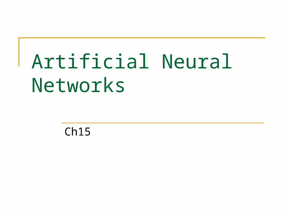
Artificial Neural Networks

Ch15

2

Objectives

Grossberg network is a self-organizing continuous-time competitive network. Continuous-time recurrent networks The foundation for the adaptive resonance theory

The biological motivation for the Grossberg network: the human visual system

3

Biological Motivation: Vision

Eyeball and Retina

Leaky Integrator

In mathematics, a leaky integrator equation is a specific differential equation, used to describe a component or system that takes the integral of an input, but gradually leaks a small amount of input over time. It appears commonly in hydraulics, electronics, and neuroscience where it can represent either a single neuron or a local population of neurons

4

5

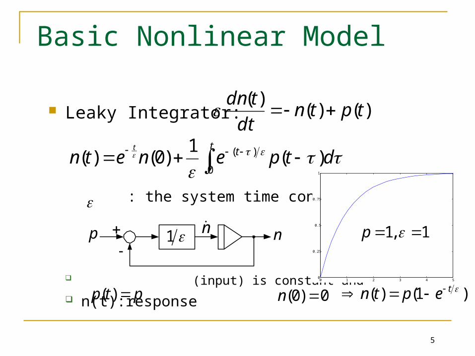
Basic Nonlinear Model

Leaky Integrator:

: the system time constant

(input) is constant and n(t):response

)()()(

tptndt

tdn

t t dtpenetnt

0

)( )(1

)0()(

1p nn

ptp )( 0)0( n )1()( teptn 0 1 2 3 4 5

0

0.25

0.5

0.75

1

1,1 p

P(t)=1

n(0)=0, = 1, 0.5, 0.25, 0.125

6

t t denetn

t

0

)(1)0()(

1)1)0(()1()0()( neenetn ttt

7

Shunting Model

Excitatory: the input that causes the response to increase –– p+. Inhibitory: the input that causes the response to decrease –– p. Biases b+ and b (nonnegative) determine the upper and lower

limits on the response.

1

p

nn

p

b

b

pbtn

ptnbtndt

tdn

)(

)()()(

btnb )(

Linear decay term

Nonlinear gain control

8

Grossberg Network

Three components:Layer 1, Layer 2 andthe adaptive weights.

The network includesshort-term memory (STM)and long-term memory(LTM) mechanisms, and performs adaptation, filtering, normalization and contrast enhancement.

Input

Layer 1(Retina)

Layer 2(Visual Cortex )

LTM(AdaptiveWeights)

STM

Normalization ConstrastEnhancement

9

Layer 1

Receives external inputs and normalizes the intensity of the input pattern.

1 nn

+W1

-W1

p

+b1

-b1

a1

pWbnpWnbnn

][)(][)()()( 1111111

1 ttt

dt

td

10

On-Center / Off-Surround

Excitatory input:

Inhibitory input:

This type of connection pattern produces a normalization of the input pattern.

100

010

001

,][ 11

WpW

011

101

110

,][ 11

WpW

11

Normalization

Inhibitory bias , Excitatory bias

Steady state neuron output

where is the relative intensity of input i.

The input vector is normalized

01 b 11 bbi

ij

jiiiii ptnptnbtndt

tdn)()()(

)( 11111

1in 0)(1 dttdni

1

1

11 ,

1

S

jj

ii pP

P

pbn iii pp

P

Pbn

1

11

Ppp ii 1

1

1

1

1

1

11

11

bP

Pbp

P

Pbn

S

jj

S

jj

12

Layer 1 Response

0 0.05 0.1 0.15 0.20

0.25

0.5

0.75

1

0 0.05 0.1 0.15 0.20

0.25

0.5

0.75

1

0.1 dn1

1t( )

dt-------------- n1

1t( )– 1 n1

1t( )– p1 n1

1t( )p2–+=

0.1 dn2

1t( )

dt-------------- n2

1t( )– 1 n2

1t( )– p2 n2

1t( )p1–+=

p128

= p21040

=

13

Characteristics of Layer 1

The network is sensitive to relative intensities of the input pattern, rather than absolute intensities.

The output of Layer 1 is a normalized version of the input pattern.

The on-center/off-surround connection pattern and the nonlinear gain control of the shunting model produce the normalization effect.

The operation of Layer 1 explains the brightness constancy and brightness contrast characteristics of the human visual system.

14

Layer 2

A layer of continuous-time instar performs several functions.

+W2W2

+b2

12n2n

-b2

a2f2

-W2

a1 On-Center

Off-Surround

15

Functions of Layer 2

It normalizes the total activity in the layer. It contrast enhances its pattern, so that the

neuron that receives the largest input will dominate the response (like winner-take-all competition in the Hamming network).

It operates as a short-term memory by storing the contrast-enhanced pattern.

16

Feedback Connections

The feedback enables the network to store a pattern, even after the input has been removed.

The feedback also performs the competition that causes the contrast enhancement of the pattern.

17

Equation of Layer 2

provides on-center feedback connection provides off-surround feedback connection W2 consists of adaptive weights. Its rows, after

training, will represent the prototype patterns. Layer 2 performs a competition between the neurons,

which tends to contrast enhance the output pattern – maintaining large outputs while attenuating small outputs.

)(][)(

)(][)()()(

22222

122222222

tt

tttdt

td

nfWbn

aWnfWnbnn

12 WW 12 WW

18

Layer 2 Example

0.1= b+ 2 1

1= b- 2 0

0= W2 w

21

T

w2

2 T

0.9 0.45

0.45 0.9= =

f2

n( )10 n

2

1 n 2+-------------------=

0.1 dn1

2t( )

dt-------------- n1

2t( )– 1 n1

2t( )– f

2n1

2t( )( ) w

21

Ta

1+

n12

t( ) f2

n22

t( )( )–+=

0.1 d n2

2t( )

dt-------------- n2

2t( )– 1 n2

2t( )– f

2n2

2t( )( ) w

22

Ta1

+

n22

t( ) f2

n12

t( )( ) .–+=

Correlation betweenprototype 1 and input.

Correlation betweenprototype 2 and input.

19

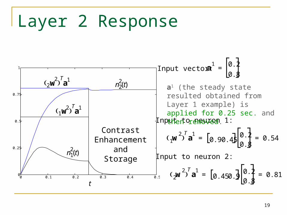
Layer 2 Response

a1 0.2

0.8=

w2

1 Ta

10.9 0.45

0.20.8

0.54= =

0 0.1 0.2 0.3 0.4 0.50

0.25

0.5

0.75

1

t

w21

Ta1

w2

2 Ta1

n12 t( )

n22 t( )

w2

2 Ta

10.45 0.9

0.20.8

0.81= =

ContrastEnhancement

andStorage

Input to neuron 1:

Input to neuron 2:

a1 (the steady state resulted obtained from Layer 1 example) is applied for 0.25 sec. and then removed.

Input vector:

20

Characteristics of Layer 2

Even before the input is removed, some contrast enhancement is performed.

After the input has been set to zero, the network further enhances the contrast and stores the patterns. It is the nonlinear feedback that enables the

network to store pattern, and the on-center/off-surround connection patterns that causes the contrast enhancement.

21

Transfer Functions

See Fig. 15.19 Linear: perfect storage of any pattern, but

amplify noise. Slower than linear: amplify noise, reduce

contrast. Faster than linear: winner-take-all, suppress

noise, quantize total activity. Sigmoid: suppress noise, contrast enhance, not

quantized.

22

Learning Law

The rows of the adaptive weights W2 will represent patterns that have been stored and that the network will be able to recognize. Long term memory (LTM)

Learning law #1:

Learning law #2:

turn off learning (and forgetting) when is NOT active.

)()()()( 122

,

2, tntntw

dt

tdwjiji

ji

decay term

Hebbian-type learning

)()()()( 12

,2

2, tntwtn

dt

tdwjjii

ji )(2 tni

23

Response of Adaptive Weights

n2 10

=

n2 01

=

For Pattern 1:

For Pattern 2:

0 0.5 1 1.5 2 2.5 30

0.25

0.5

0.75

1

w1 12 t( )

w1 22 t( )

w2 12 t( )

w2 22 t( )

The first row of the weight matrix is updated when n1

2(t) is active, and

the second row of the weight matrix is updated when n2

2(t) is active.

Two different input patterns are alternately presented to the network for periods of 0.2 seconds at a time.

n1 0.90.45

=

n1 0.450.9

=

24

Relation to Kohonen Law

Grossberg learning law (continuous-time):

Euler approximation for the derivative:

Discrete-time approximation to Grossberg law:

d w2i t( ) dt

---------------------- ni2

t( ) w2i t( ) – n1

t( )+ =

d w2i t( ) dt

----------------------w2

i t t+( ) w2i t( )–

t----------------------------------------------

w2i t t+( ) w2

i t( ) t ni2

t( ) w2i t( )– n1

t( )+ +=

25

Relation to Kohonen Law

Rearrange terms:

Assume that a faster-than-linear transfer function (winner-take-all) is used in Layer 2.

Kohonen law:

w2

i t t+( ) 1 t ni2

t( )– w2

i t( ) t ni2

t( ) n1

t( ) +=

w2

i t t+( ) 1 '– w2

i t( ) 'n1

t( )+= ' t ni2

t( )=

wi q 1 – w

i q 1– p q +=

26

Three Major Differences

The Grossberg network is a continuous-time network.

Layer 1 of Grossberg network automatically normalizes the input vectors.

Layer 2 of Grossberg network can perform a “soft” competition, rather than the winner-take-all competition of the Kohonen network. This soft competition allows more than one neuron in

Layer 2 to learn. Cause the Grossberg network to operate as a feature

map.