Artificial Artificial Intelligence for Intelligence for Data Mining in Data Mining in the Context of the Context of

Enterprise Enterprise SystemsSystemsThesis Presentation byThesis Presentation by

Real CarbonneauReal Carbonneau

OverviewOverview

BackgroundBackground Research QuestionResearch Question Data SourcesData Sources MethodologyMethodology ImplementationImplementation ResultsResults ConclusionConclusion

BackgroundBackground

Information distortion in the supply chainInformation distortion in the supply chain Difficult for manufacturers to forecastDifficult for manufacturers to forecast

Distributor

$ $

$

CustomerManufacturer RetailerWholesaler

OrderOrderOrderOrder

Information flow in the extended supply chainCollaboration Barrier

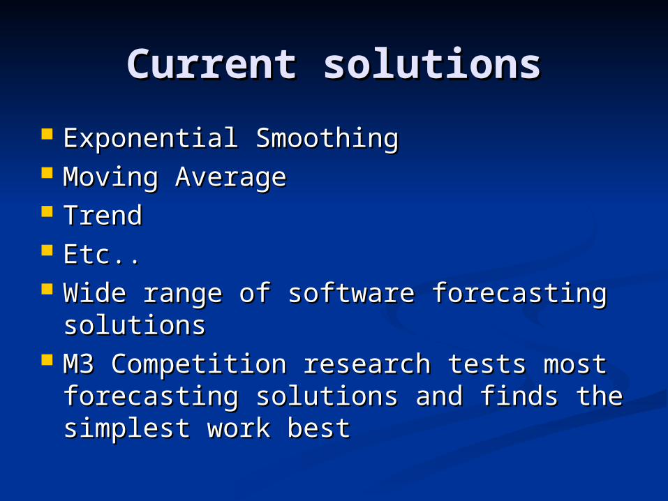
Current solutionsCurrent solutions

Exponential SmoothingExponential Smoothing Moving AverageMoving Average TrendTrend Etc..Etc.. Wide range of software forecasting Wide range of software forecasting

solutionssolutions M3 Competition research tests most M3 Competition research tests most

forecasting solutions and finds the forecasting solutions and finds the simplest work bestsimplest work best

Artificial IntelligenceArtificial Intelligence

Universal ApproximatorsUniversal Approximators Artificial Neural Networks (ANN)Artificial Neural Networks (ANN) Recurrent Neural Networks (RNN)Recurrent Neural Networks (RNN) Support Vector Machines (SVM)Support Vector Machines (SVM)

Theorectically should be able to Theorectically should be able to match or outperform any traditional match or outperform any traditional forecasting approach.forecasting approach.

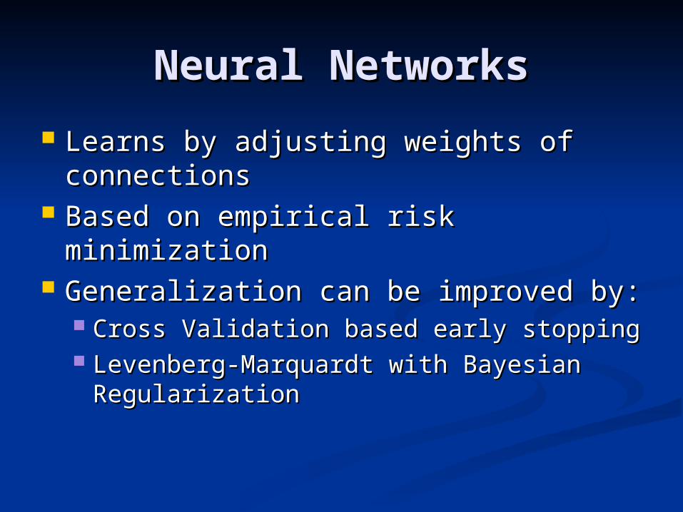
Neural NetworksNeural Networks

Learns by adjusting weights of Learns by adjusting weights of connectionsconnections

Based on empirical risk minimizationBased on empirical risk minimization Generalization can be improved by:Generalization can be improved by:

Cross Validation based early stoppingCross Validation based early stopping Levenberg-Marquardt with Bayesian Levenberg-Marquardt with Bayesian

RegularizationRegularization

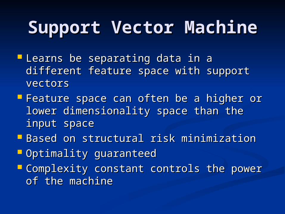
Support Vector MachineSupport Vector Machine

Learns be separating data in a different Learns be separating data in a different feature space with support vectorsfeature space with support vectors

Feature space can often be a higher or Feature space can often be a higher or lower dimensionality space than the lower dimensionality space than the input spaceinput space

Based on structural risk minimizationBased on structural risk minimization Optimality guaranteed Optimality guaranteed Complexity constant controls the power Complexity constant controls the power

of the machineof the machine

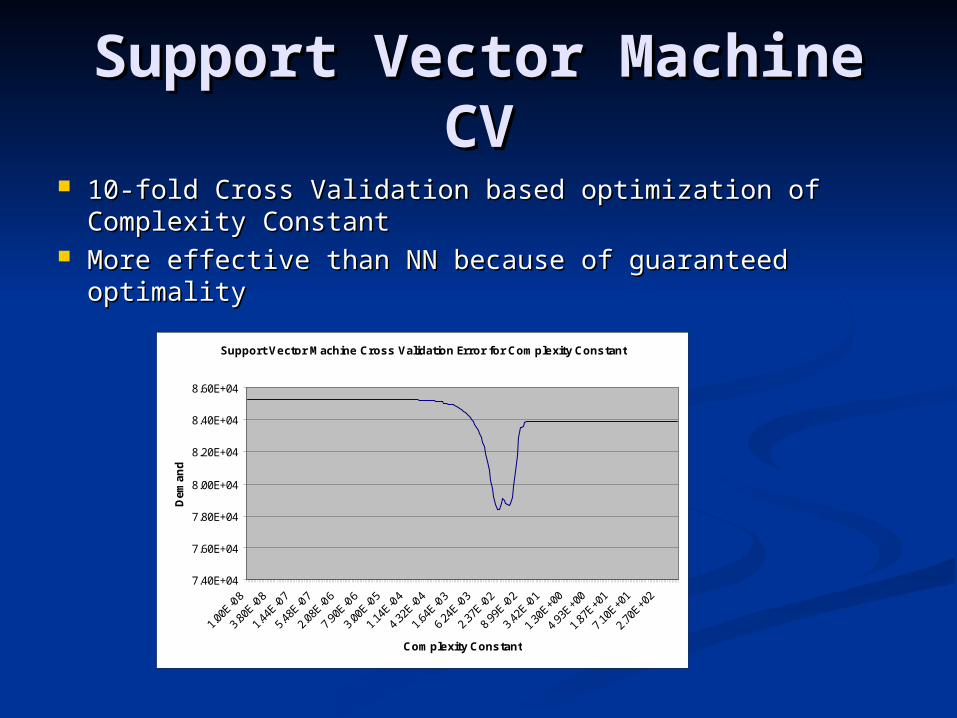
Support Vector Machine Support Vector Machine CVCV

10-fold Cross Validation based optimization of 10-fold Cross Validation based optimization of Complexity ConstantComplexity Constant

More effective than NN because of guaranteed optimalityMore effective than NN because of guaranteed optimality

Support Vector Machine Cross Validation Error for Complexity Constant

7.40E+04

7.60E+04

7.80E+04

8.00E+04

8.20E+04

8.40E+04

8.60E+04

1.00

E-08

3.80

E-08

1.44

E-07

5.48

E-07

2.08

E-06

7.90

E-06

3.00

E-05

1.14

E-04

4.32

E-04

1.64

E-03

6.24

E-03

2.37

E-02

8.99

E-02

3.42

E-01

1.30

E+00

4.93

E+00

1.87

E+01

7.10

E+01

2.70

E+02

Complexity Constant

Dem

and

SVM Complexity ExampleSVM Complexity Example

SVM Complexity Constant SVM Complexity Constant optimization based on 10-Fold Cross optimization based on 10-Fold Cross ValidationValidationSupport Vector Machine Forecasts with varying Complexity Constants

0.00E+00

5.00E+04

1.00E+05

1.50E+05

2.00E+05

2.50E+05

3.00E+05

3.50E+05

1 3 5 7 9 11 13 15 17 19 21 23

Period

Dem

and

Actual

High Complexity

Low Complexity

Optimal Complexity

Research QuestionResearch Question

For a manufacturer at the end of the For a manufacturer at the end of the supply chain who is subject to supply chain who is subject to demand distortion:demand distortion: H1: Are AI approaches better on average H1: Are AI approaches better on average

than traditional approaches (error)than traditional approaches (error) H2: Are AI approaches better than H2: Are AI approaches better than

traditional approaches (rank)traditional approaches (rank) H3: Is the best AI approach better than H3: Is the best AI approach better than

the best traditionalthe best traditional

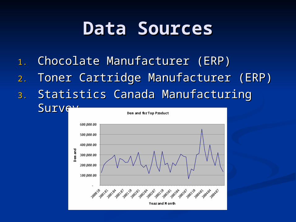
Data SourcesData Sources

1.1. Chocolate Manufacturer (ERP)Chocolate Manufacturer (ERP)

2.2. Toner Cartridge Manufacturer (ERP)Toner Cartridge Manufacturer (ERP)

3.3. Statistics Canada Manufacturing SurveyStatistics Canada Manufacturing SurveyDemand for Top Product

-

100,000.00

200,000.00

300,000.00

400,000.00

500,000.00

600,000.00

Year and Month

Dem

and

MethodoloyMethodoloy

ExperimentExperiment Using top 100 from 2 manufacturers Using top 100 from 2 manufacturers

and random 100 from StatsCanand random 100 from StatsCan Comparison based on out-of-sample Comparison based on out-of-sample

testing settesting set

ImplementationImplementation

Experiment programmed in MATLABExperiment programmed in MATLAB Using existing toolbox where Using existing toolbox where

possible (eg, NN, ARMA, etc)possible (eg, NN, ARMA, etc) Programming missing onesProgramming missing ones SVM implemented using mySVM SVM implemented using mySVM

called from MATLABcalled from MATLAB

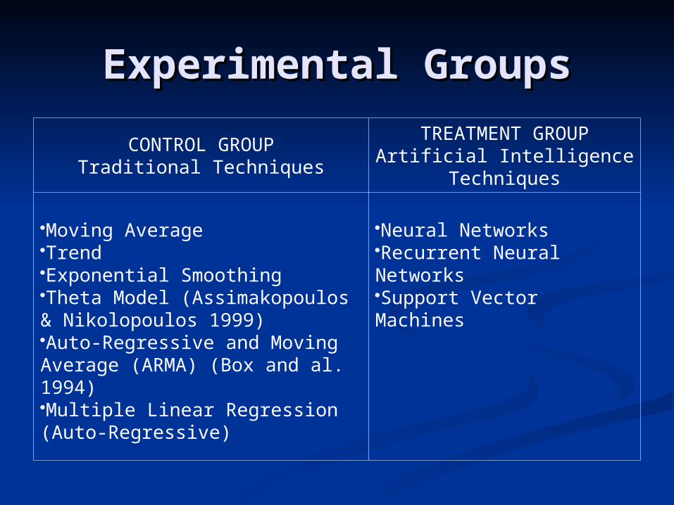
Experimental GroupsExperimental Groups

CONTROL GROUPTraditional Techniques

TREATMENT GROUPArtificial Intelligence

Techniques

Moving AverageTrendExponential SmoothingTheta Model (Assimakopoulos & Nikolopoulos 1999)Auto-Regressive and Moving Average (ARMA) (Box and al. 1994)Multiple Linear Regression (Auto-Regressive)

Neural NetworksRecurrent Neural NetworksSupport Vector Machines

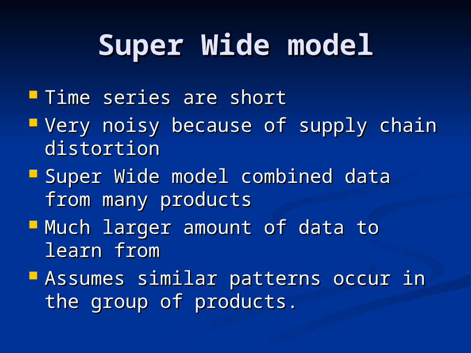
Super Wide modelSuper Wide model

Time series are shortTime series are short Very noisy because of supply chain Very noisy because of supply chain

distortiondistortion Super Wide model combined data Super Wide model combined data

from many productsfrom many products Much larger amount of data to learn Much larger amount of data to learn

fromfrom Assumes similar patterns occur in the Assumes similar patterns occur in the

group of products.group of products.

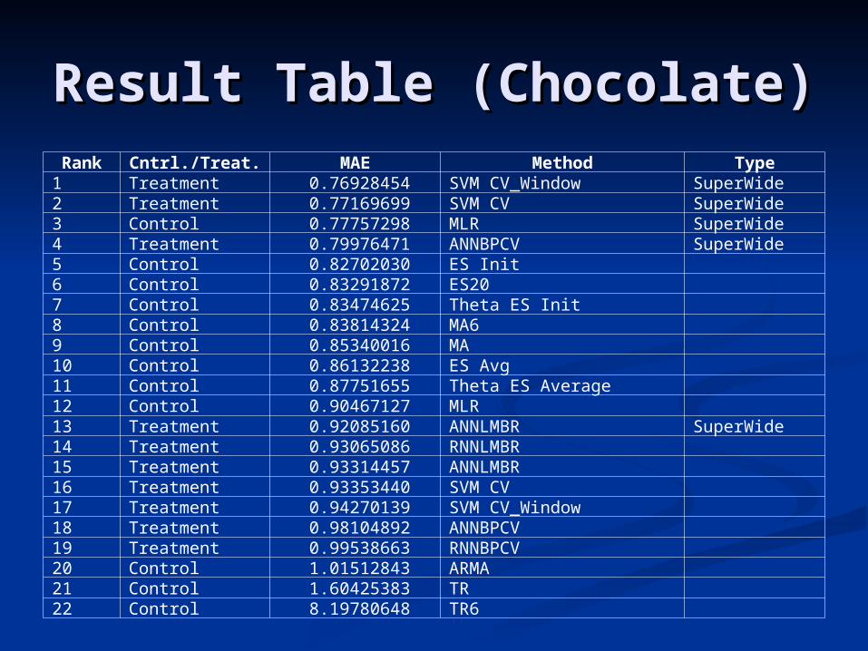
Result Table (Chocolate)Result Table (Chocolate)Rank Cntrl./Treat. MAE Method Type

1 Treatment 0.76928454 SVM CV_Window SuperWide2 Treatment 0.77169699 SVM CV SuperWide3 Control 0.77757298 MLR SuperWide4 Treatment 0.79976471 ANNBPCV SuperWide5 Control 0.82702030 ES Init6 Control 0.83291872 ES207 Control 0.83474625 Theta ES Init8 Control 0.83814324 MA69 Control 0.85340016 MA10 Control 0.86132238 ES Avg11 Control 0.87751655 Theta ES Average12 Control 0.90467127 MLR 13 Treatment 0.92085160 ANNLMBR SuperWide14 Treatment 0.93065086 RNNLMBR15 Treatment 0.93314457 ANNLMBR16 Treatment 0.93353440 SVM CV17 Treatment 0.94270139 SVM CV_Window18 Treatment 0.98104892 ANNBPCV19 Treatment 0.99538663 RNNBPCV20 Control 1.01512843 ARMA21 Control 1.60425383 TR22 Control 8.19780648 TR6

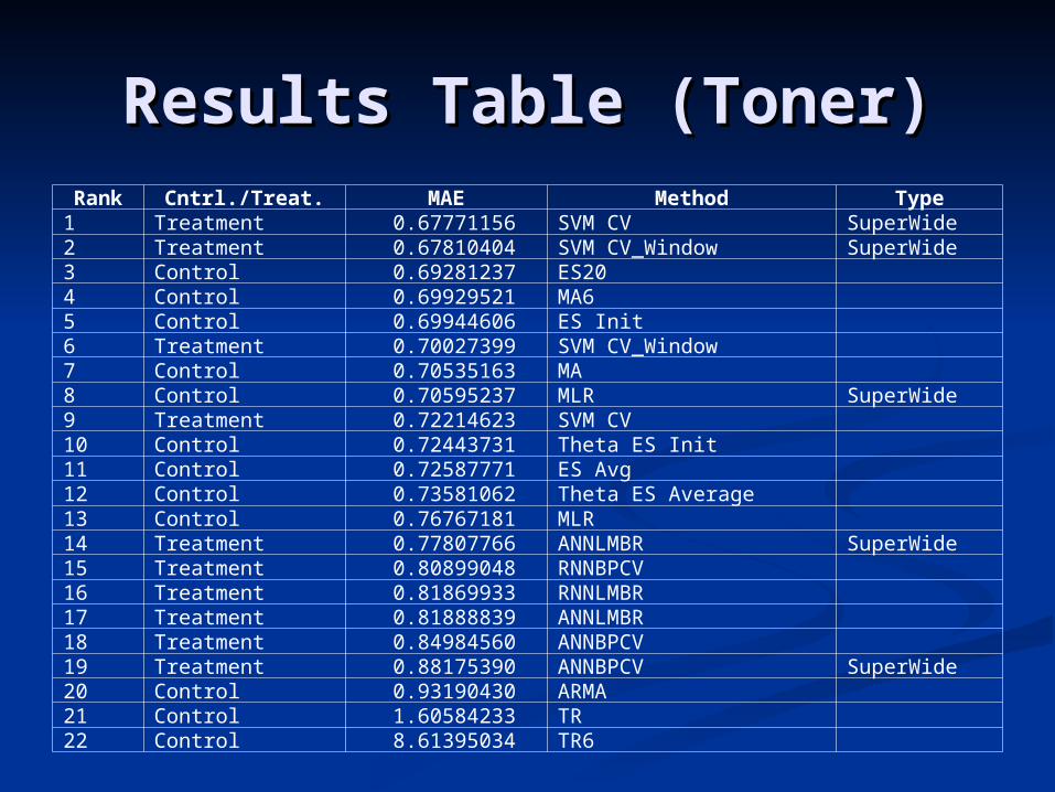
Results Table (Toner)Results Table (Toner)Rank Cntrl./Treat. MAE Method Type

1 Treatment 0.67771156 SVM CV SuperWide2 Treatment 0.67810404 SVM CV_Window SuperWide3 Control 0.69281237 ES204 Control 0.69929521 MA65 Control 0.69944606 ES Init6 Treatment 0.70027399 SVM CV_Window7 Control 0.70535163 MA8 Control 0.70595237 MLR SuperWide9 Treatment 0.72214623 SVM CV10 Control 0.72443731 Theta ES Init11 Control 0.72587771 ES Avg12 Control 0.73581062 Theta ES Average13 Control 0.76767181 MLR 14 Treatment 0.77807766 ANNLMBR SuperWide15 Treatment 0.80899048 RNNBPCV16 Treatment 0.81869933 RNNLMBR17 Treatment 0.81888839 ANNLMBR18 Treatment 0.84984560 ANNBPCV19 Treatment 0.88175390 ANNBPCV SuperWide20 Control 0.93190430 ARMA21 Control 1.60584233 TR22 Control 8.61395034 TR6

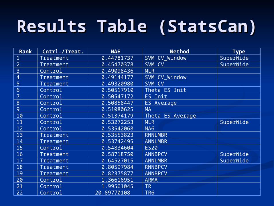
Results Table (StatsCan)Results Table (StatsCan)Rank Cntrl./Treat. MAE Method Type

1 Treatment 0.44781737 SVM CV_Window SuperWide2 Treatment 0.45470378 SVM CV SuperWide3 Control 0.49098436 MLR 4 Treatment 0.49144177 SVM CV_Window5 Treatment 0.49320980 SVM CV6 Control 0.50517910 Theta ES Init7 Control 0.50547172 ES Init8 Control 0.50858447 ES Average9 Control 0.51080625 MA10 Control 0.51374179 Theta ES Average11 Control 0.53272253 MLR SuperWide12 Control 0.53542068 MA613 Treatment 0.53553823 RNNLMBR14 Treatment 0.53742495 ANNLMBR15 Control 0.54834604 ES2016 Treatment 0.58718750 ANNBPCV SuperWide17 Treatment 0.64527015 ANNLMBR SuperWide18 Treatment 0.80597984 RNNBPCV19 Treatment 0.82375877 ANNBPCV20 Control 1.36616951 ARMA21 Control 1.99561045 TR22 Control 20.89770108 TR6

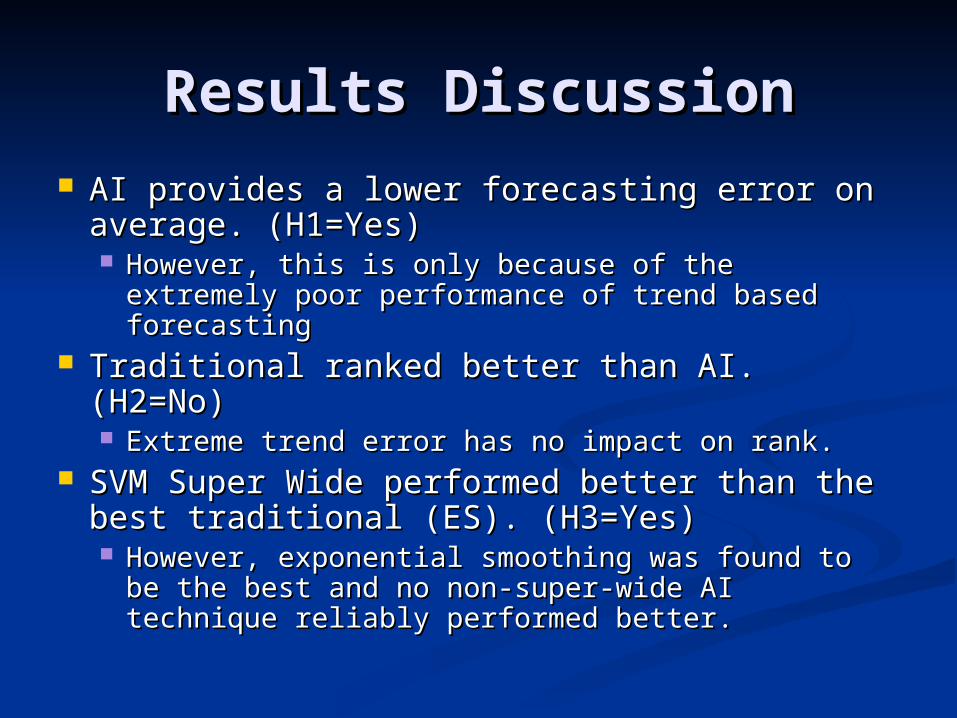
Results DiscussionResults Discussion AI provides a lower forecasting error on AI provides a lower forecasting error on

average. (H1=Yes) average. (H1=Yes) However, this is only because of the extremely However, this is only because of the extremely

poor performance of trend based forecastingpoor performance of trend based forecasting Traditional ranked better than AI. (H2=No) Traditional ranked better than AI. (H2=No)

Extreme trend error has no impact on rank.Extreme trend error has no impact on rank.

SVM Super Wide performed better than SVM Super Wide performed better than the best traditional (ES). (H3=Yes) the best traditional (ES). (H3=Yes) However, exponential smoothing was found to However, exponential smoothing was found to

be the best and no non-super-wide AI technique be the best and no non-super-wide AI technique reliably performed better.reliably performed better.

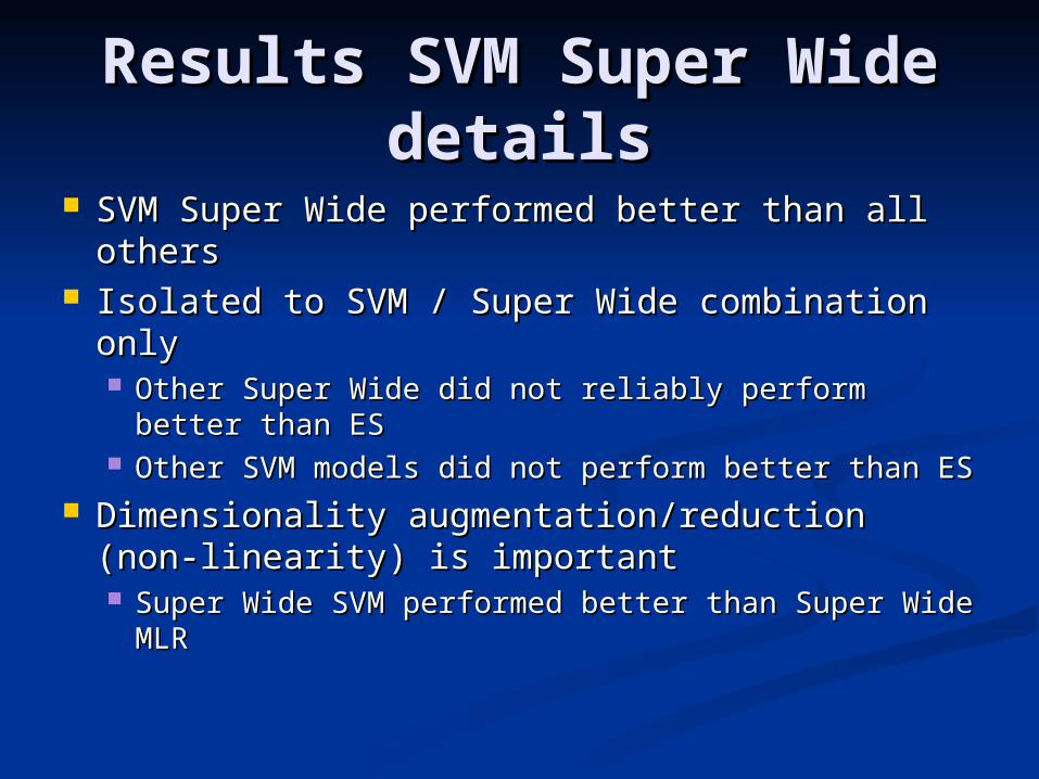
Results SVM Super Wide Results SVM Super Wide detailsdetails

SVM Super Wide performed better than all SVM Super Wide performed better than all othersothers

Isolated to SVM / Super Wide combination Isolated to SVM / Super Wide combination onlyonly Other Super Wide did not reliably perform better Other Super Wide did not reliably perform better

than ESthan ES Other SVM models did not perform better than ESOther SVM models did not perform better than ES

Dimensionality augmentation/reduction (non-Dimensionality augmentation/reduction (non-linearity) is importantlinearity) is important Super Wide SVM performed better than Super Super Wide SVM performed better than Super

Wide MLRWide MLR

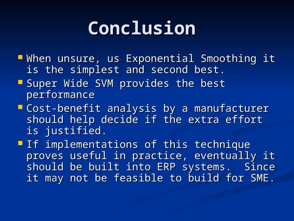
Conclusion Conclusion When unsure, us Exponential Smoothing it When unsure, us Exponential Smoothing it

is the simplest and second best.is the simplest and second best. Super Wide SVM provides the best Super Wide SVM provides the best

performanceperformance Cost-benefit analysis by a manufacturer Cost-benefit analysis by a manufacturer

should help decide if the extra effort is should help decide if the extra effort is justified.justified.

If implementations of this technique proves If implementations of this technique proves useful in practice, eventually it should be useful in practice, eventually it should be built into ERP systems. Since it may not built into ERP systems. Since it may not be feasible to build for SME.be feasible to build for SME.

ImplicationsImplications

Useful for forecasting models which Useful for forecasting models which should include more information sources should include more information sources / more variables (Economic indicators, / more variables (Economic indicators, product group performances, marketing product group performances, marketing campaigns) because:campaigns) because: Super Wide = More observationsSuper Wide = More observations SVM+CV = Better GeneralizationSVM+CV = Better Generalization

Not possible with short and noisy time Not possible with short and noisy time series on their own.series on their own.