article ship-iceberg discrimination in sentinel-

Remote Sens. 2017, 9, x; doi: FOR PEER REVIEW www.mdpi.com/journal/remotesensing

Article 1

Ship-Iceberg Discrimination in Sentinel-2 2

Multispectral Imagery by Supervised Classification 3

Peder Heiselberg 1 and Henning Heiselberg 2,* 4

1 Climate & Geophysics, Niels Bohr Institute, Juliane Maries Vej 30, 2100 Copenhagen Ø, Denmark; 5 [email protected] 6

2 National Space Institute, Technical University of Denmark, 2800 Kongens Lyngby, Denmark 7 * Correspondence: [email protected]. Tel.: +45-45259760 8

Academic Editor: name 9 Received: date; Accepted: date; Published: date 10

Abstract: The European Space Agency Sentinel-2 satellites provide multispectral images with pixel 11 sizes down to 10 m. This high resolution allows for fast and frequent detection, classification and 12 discrimination of various objects in the sea, which is relevant in general and specifically for the vast 13 Arctic environment. We analyze several sets of multispectral image data from Denmark and 14 Greenland fall and winter, and describe a supervised search and classification algorithm based on 15 physical parameters that successfully finds and classifies all objects in the sea with reflectance above 16 a threshold. It discriminates between objects like ships, islands, wakes, and icebergs, ice floes, and 17 clouds with accuracy better than 90%. Pan-sharpening the infrared bands leads to classification and 18 discrimination of ice floes and clouds better than 95%. For complex images with abundant ice floes 19 or clouds, however, the false alarm rate dominates for small non-sailing boats. 20

Keywords: Sentinel-2; multispectral; ship; iceberg; detection; discrimination; classification; Arctic 21 22

1. Introduction 23

Marine surveillance and situation awareness is essential for monitoring and controlling piracy, 24 smuggling, fishing, irregular migration, trespassing, spying, traffic safety, icebergs, sea ice, 25 shipwrecks, the environment (oil spill or pollution), etc. Black ships are non-cooperative ships with 26 non-functioning transponder systems. Their transmission may be jammed, spoofed, sometimes 27 experience erroneous returns, or are simply turned off deliberately or by accident. Furthermore, AIS 28 satellite coverage at high latitudes is sparse, which means that other non-cooperative surveillance 29 systems, including satellite or airborne systems, are required. 30

The Sentinel satellites under the Copernicus program [1] provide excellent and freely available 31 multispectral imagery with resolutions down to 10 m in four bands, and Synthetic Aperture Radar 32 primarily with resolution down to 90 m in the high resolution extra wide swath ground range 33 detection mode. Their frequent transits over the polar regions make these satellites particularly 34 useful for Artic surveillance and for monitoring icebergs, sea-ice coverage [2,3], ships [4–17], 35 oil spills [18–20], crop and forestation [21,22]. 36

The orbital period is 10 days for the Sentinel-2 (S2) satellites A + B, each of which carries 37 multispectral imaging (MSI) instruments. The image strips overlap at a given point on the Earth, and 38 the typical revisit period for each satellite is two or three days in Europe and almost daily in the 39 Arctic. S2 MSI has the potential to greatly improve the marine situational awareness, especially for 40 non-cooperative ships—weather permitting. 41

The Iceberg Alley [3] is a dangerous iceberg infested route running from west Greenland and 42 Baffin Island and Newfoundland, down into a strait where many ships, including the Titanic, transit 43 the North Atlantic. In September 2016, Crystal Serenity was the first cruise ship that risked sailing 44

Remote Sens. 2017, 9, x FOR PEER REVIEW 2 of 19

from Alaska to Greenland through the Northwest Passage, which is infested with uncharted reefs, 45 sea ice and huge icebergs. Since satellite AIS coverage is very limited at these latitudes, ships are 46 essentially non-cooperative in the Arctic. 47

SAR imagery [2–6] is weather independent, but generally has lower resolution, is subject to 48 speckle noise, motion blurring, and has target and angle dependent reflection coefficients. SAR is 49 therefore less useful for small ship detection and classification. In addition, SAR is unable to detect 50 objects with low dielectric coefficients as wooden or glass fiber boats. The high resolution S2 MSI can, 51 as is shown below, improve the classification, discrimination and multispectral identification of ships 52 and threats from icebergs, unless clouds cover the sea. 53

This article focuses on search, classification and discrimination of ships, islands, icebergs, sea 54 ice, wakes and clouds in S2 MSI. For this reason, two regions of interest have been selected: Skagen 55 on the northernmost tip of Denmark, where there are often a large number of ships, boats, wakes and 56 clouds, and Nuuk the capital of Greenland where there are numerous fishing boats, icebergs and ice 57 floes. The classification method is based on elements of principal component analyses (PCA) and also 58 k-method algorithms [23]. The analysis identifies the most useful aspects of these methods, and 59 provides a direct physical understanding and classification of the objects to be found and 60 discriminated in Arctic and other environments. Based on this analysis, a supervised classification 61 algorithm is developed that exploits both the spatial and spectral information in the multispectral 62 images from S2 MSI. 63

Detection is relatively easy due to the high sensitivity and dynamic range of the images, and the 64 generally dark sea background. Recognition is based on high-resolution images that allow for an 65 accurate and robust classification of objects from the spatial and spectral information. The accuracy 66 and confidence of all of this is fundamentally reliant on the target’s spectral reflectances and size. The 67 analysis and discussion of the accuracy of the recognition and identification, based on a target’s S2 68 MSI data, are obtained as outputs from the S2 MSI detection, recognition and identification process. 69

The paper is organized such that the S2 data are described first, followed by a description of the 70 data analysis. Subsequently, the classification model is described based on spatial and spectral 71 characteristic of the objects, followed by a presentation of the results for classification of ships, 72 islands, icebergs, grey ice, wakes, etc. including a discussion of the confusion matrix and false alarms. 73 Finally, a summary and outlook are also offered. 74

2. Satellite Images and Method of Analysis 75

The S2 multispectral images are analyzed by using dedicated software developed for the 76 purpose of small object classification in large images in several multispectral bands with different 77 pixel resolutions. The images have been preprocessed by the sen2cor algorithm for atmospheric 78 corrections [24]. The processing is mainly designed for object search and classification, and is fast (a 79 few seconds) depending on the size and complexity of the mega- to giga-pixel images with 4048 (12 80 bit) grey levels. We will describe in detail how the segments are detected, and how their multispectral 81 reflectances and several spatial properties are calculated. 82

Subsequently, we describe a supervised classification of the segments as objects based on both 83 spatial and spectral properties that are related to physical properties of the objects. The classification 84 is based on—but not restricted to—standard methods from principal components analysis (PCA), 85 k-means and Mahalonobis distances [23], but is tailored specifically to optimize the classification of 86 smaller ships and icebergs. The success of the classification method lies in choosing the best classifiers 87 and thresholds that correctly identify most segments. 88

2.1. Sentinel-2 Multispectral Images 89

S2 carries the wide-swath, high-resolution, multispectral imager (MSI) with 13 spectral bands 90 with 10, 20 or 60 m resolution [1]. As we are interested in detailed small object classification and 91 discrimination, we will focus on analyzing the four bands with 10 m resolution, namely B2 (blue), B3 92 (green), B4 (red) and B8 (near-infrared). In addition, the two short wave infrared bands B11 and B12 93 with 20 m resolution are pan-sharpened and included. 94


Two regions of interest are selected: Skagen, the northernmost tip of Denmark (Figure 1), and 95 Nuuk, the capital of Greenland (Figure 2). These images are convenient for classification because the 96 objects are relatively easy to identify as there is only ice and a few islands and sailing fishing boats in 97 Nuuk. In contrast, a number of large ships, smaller boats, wakes and clouds are present at Skagen. 98 The S2 images analyzed here are recorded over Skagen on 23 August 2016 shown in Figure 1 (with 99 analyses in Figures 3-6) and excerpts of Figure 1 in Figures 7.a+b. The S2 images over Nuuk are from 100 23 September (Figure 2), 16 October (Figure 8.a) and 23 October (Figure 8.b with analysis in Figure 101 9), all in 2016. Nuuk is situated on 64° north latitude just below the polar circle. S2 passes over Nuuk 102 around noon, therefore there is always light all year around, although shadows can be long during 103 winter. S2 data over Nuuk are processed and made available with a few days interval except in 104 December and January. Finally in Figure 10 we return to a cloudy image over Skagen from 1 105 September 2016. 106

107

Figure 1. Copernicus Sentinel-2A data [5 September 2016 at 10:30 a.m. UTC]. Southwest corner of 108 Sentinel-2A image tile VNK showing Skagen—the northernmost tip of Denmark. The image is RGB 109 contrast-enhanced so that large ships are visible but land is almost saturated. Left white box contains 110 a fleet of fishing ships located in Skagerak west of Skagen (see Figure 7a). Right white box contains a 111 number of container and tanker ships en route around Skagen and moored just east of Skagen in the 112 tranquil sea of Kattegat (see Figure 7b), a number of which are waiting for bulk fuel. 113

The images contain reflectances IBx(i,j) for each of the 13 multispectral bands x = 1, …, 8, 8A, 9, 114 10, 11, 12. The pixel coordinates (i,j) are the (x,y) coordinates in units of the pixel resolution l, which 115 is l = 10 m for the blue, green, red and near-infrared bands B2, B3, B4, and B8, respectively; l = 20 m 116 for B5, B6, B7, B8A, B11, and B12; and l = 60 m for B1, B9, and B10. 117

To detect an object, its reflectance must deviate from the sea background in one or more spectral 118 bands. Most objects we have encountered reflect more light in all bands than the sea and we therefore 119 subtract the sea background in all spectral bands. For resolving the objects optimally, we sum the 120 reflectances in the four high-resolution bands B2 + B3 + B4 + B8 with sea background subtracted 121

I4(𝑖, 𝑗) = IB2(𝑖, 𝑗) + IB3(𝑖, 𝑗) + IB4(𝑖, 𝑗) + IB8(𝑖, 𝑗) − background . (1)

Since the sea covered substantially more than half of the area in all our images, the median 122 reflectance value for each images provided an accurate and robust value for the background. This 123 total reflectance image I4 has the highest resolution and contrast to the sea and is therefore optimal 124 for object search and detection. 125

To be seen, the object must exceed a threshold which depends on the scenario. Examples of the 126 threshold dependence are shown in Figure 3 and discussed in the following subsection. In normal 127 sea background, the threshold can be chosen rather low, whereas in icy Arctic oceans with 128


widespread ice floes or images with clouds, it may be advantageous to choose a higher threshold in 129 order to distinguish objects from ice floes and clouds. Thereby the false alarm rate for ship detection 130 is much reduced as the large number ice floes with high spatial and spectral variation is suppressed. 131 However, as a result, we risk that, e.g., small and slow ships are “hidden” in a background of ice 132 floes, as will be discussed later. 133

134

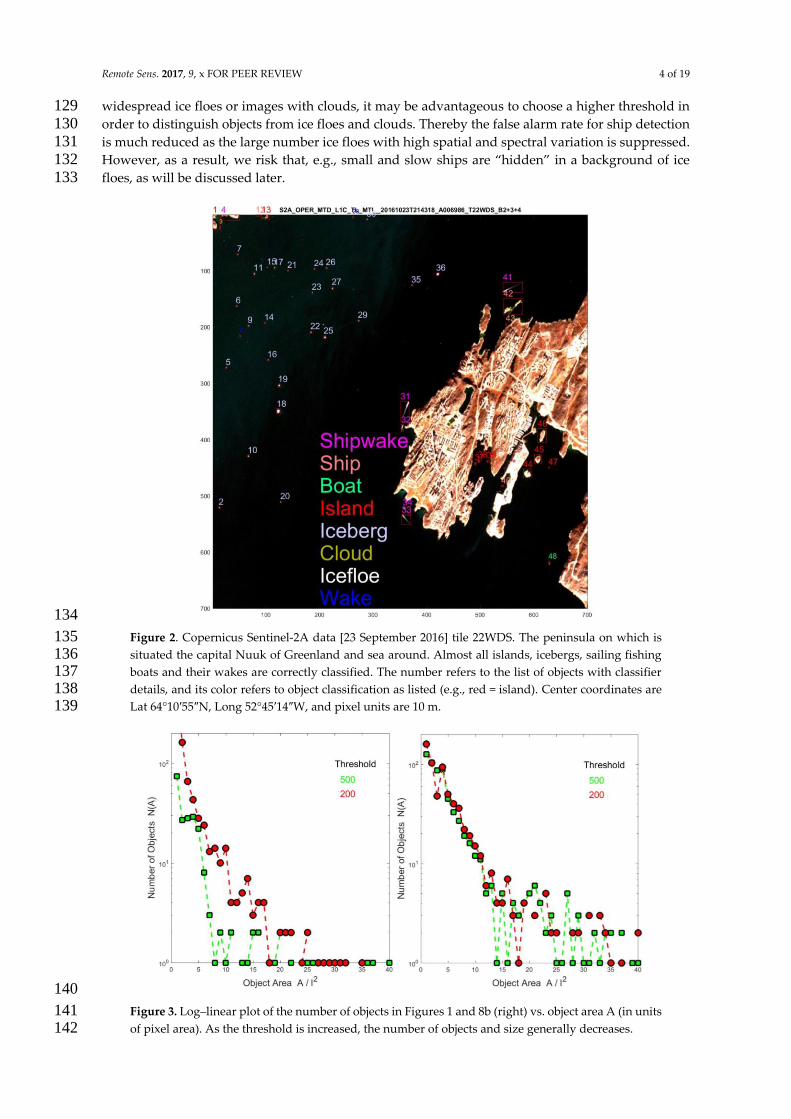
Figure 2. Copernicus Sentinel-2A data [23 September 2016] tile 22WDS. The peninsula on which is 135 situated the capital Nuuk of Greenland and sea around. Almost all islands, icebergs, sailing fishing 136 boats and their wakes are correctly classified. The number refers to the list of objects with classifier 137 details, and its color refers to object classification as listed (e.g., red = island). Center coordinates are 138 Lat 64°10′55″N, Long 52°45′14″W, and pixel units are 10 m. 139

140

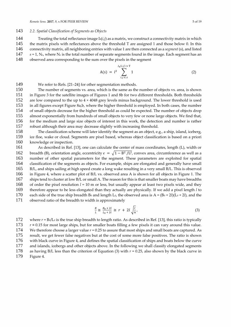
Figure 3. Log–linear plot of the number of objects in Figures 1 and 8b (right) vs. object area A (in units 141 of pixel area). As the threshold is increased, the number of objects and size generally decreases. 142


2.2. Spatial Classification of Segments as Objects 143

Treating the total reflectance image I4(i,j) as a matrix, we construct a connectivity matrix in which 144 the matrix pixels with reflectances above the threshold T are assigned 1 and those below 0. In this 145 connectivity matrix, all neighboring entries with value 1 are then connected as a segment (s), and listed 146 s = 1, Ns, where Ns is the total number of separate segments found in the image. Each segment has an 147 observed area corresponding to the sum over the pixels in the segment 148

A(s) = 𝑙2 ∑ 1

𝐼4(𝑖,𝑗) > T

𝑖,𝑗 ∈ 𝑠

(2)

We refer to Refs. [21–24] for other segmentation methods. 149 The number of segments vs. area, which is the same as the number of objects vs. area, is shown 150

in Figure 3 for the satellite images of Figures 1 and 8b for two different thresholds. Both thresholds 151 are low compared to the up to 4 × 4048 grey levels minus background. The lower threshold is used 152 in all figures except Figure 8a,b, where the higher threshold is employed. In both cases, the number 153 of small objects decrease for the higher threshold as could be expected. The number of objects drop 154 almost exponentially from hundreds of small objects to very few or none large objects. We find that, 155 for the medium and large size objects of interest in this work, the detection and number is rather 156 robust although their area may decrease slightly with increasing threshold. 157

The classification scheme will later identify the segment as an object, e.g., a ship, island, iceberg, 158 ice floe, wake or cloud. Segments are pixel based, whereas object classification is based on a priori 159 knowledge or inspection. 160

As described in Ref. [13], one can calculate the center of mass coordinates, length (L), width or 161

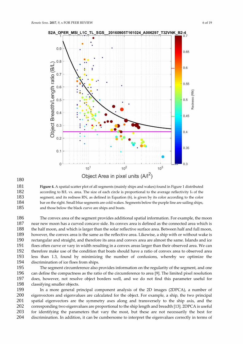
breadth (B), orientation angle, eccentricity 𝜖 = √1 − B2 /L2, convex area, circumference as well as a 162 number of other spatial parameters for the segment. These parameters are exploited for spatial 163 classification of the segments as objects. For example, ships are elongated and generally have small 164 B/L, and ships sailing at high speed create a long wake resulting in a very small B/L. This is observed 165 in Figure 4, where a scatter plot of B/L vs. observed area A is shown for all objects in Figure 1. The 166 ships tend to cluster at low B/L or small A. The reason for this is that smaller boats may have breadths 167 of order the pixel resolution l = 10 m or less, but usually appear at least two pixels wide, and they 168 therefore appear to be less elongated than they actually are physically. If we add a pixel length l to 169 each side of the true ship breadth B0 and length L0, the observed area is A = (B0 + 2l)(L0 + 2l), and the 170 observed ratio of the breadth to width is approximately 171

𝐵

𝐿≅

𝐵0 + 2𝑙

𝐿0 + 2𝑙 ≅ 𝑟 + 2𝑙 √

𝑟

A , (3)

where r = B0/L0 is the true ship breadth to length ratio. As described in Ref. [13], this ratio is typically 172 r ≅ 0.15 for most large ships, but for smaller boats filling a few pixels it can vary around this value. 173 We therefore choose a larger value r = 0.25 to assure that most ships and small boats are captured. As 174 result, we get fewer false negatives but at the cost of some more false positives. The ratio is shown 175 with black curve in Figure 4, and defines the spatial classification of ships and boats below the curve 176 and islands, icebergs and other objects above. In the following we shall classify elongated segments 177 as having B/L less than the criterion of Equation (3) with r = 0.25, also shown by the black curve in 178 Figure 4. 179


180

Figure 4. A spatial scatter plot of all segments (mainly ships and wakes) found in Figure 1 distributed 181 according to B/L vs. area. The size of each circle is proportional to the average reflectivity I4 of the 182 segment, and its redness RN, as defined in Equation (6), is given by its color according to the color 183 bar on the right. Small blue segments are cold wakes. Segments below the purple line are sailing ships, 184 and those below the black curve are ships and boats. 185

The convex area of the segment provides additional spatial information. For example, the moon 186 near new moon has a curved concave side. Its convex area is defined as the connected area which is 187 the half moon, and which is larger than the solar reflective surface area. Between half and full moon, 188 however, the convex area is the same as the reflective area. Likewise, a ship with or without wake is 189 rectangular and straight, and therefore its area and convex area are almost the same. Islands and ice 190 floes often curve or vary in width resulting in a convex areas larger than their observed area. We can 191 therefore make use of the condition that boats should have a ratio of convex area to observed area 192 less than 1.3, found by minimizing the number of confusions, whereby we optimize the 193 discrimination of ice floes from ships. 194

The segment circumference also provides information on the regularity of the segment, and one 195 can define the compactness as the ratio of the circumference to area [9]. The limited pixel resolution 196 does, however, not resolve object borders well, and we do not find this parameter useful for 197 classifying smaller objects. 198

In a more general principal component analysis of the 2D images (2DPCA), a number of 199 eigenvectors and eigenvalues are calculated for the object. For example, a ship, the two principal 200 spatial eigenvectors are the symmetry axes along and transversely to the ship axis, and the 201 corresponding two eigenvalues are proportional to the ship length and breadth [13]. 2DPCA is useful 202 for identifying the parameters that vary the most, but these are not necessarily the best for 203 discrimination. In addition, it can be cumbersome to interpret the eigenvalues correctly in terms of 204


physical parameters and for classification. We therefore use the principal components only as a 205 guideline for selecting the physical parameters most useful for classification. 206

A very useful classification method is k-means clustering or k-nearest neighbor, where k objects are 207 assigned a number of classifiers [23]. For example, a ship should have small B/L and area A smaller 208 than ca. 300 pixels (30,000 m2) but convex area not much larger than its area, as well as spectral 209 properties discussed below. A segment is classified to that object which deviates least from its 210 classifiers, i.e., the object that the segment resembles the most. Least deviation can be defined in a 211 number of ways, e.g., as a weighted least mean square value. We shall employ a more direct and 212 sharp classification algorithm that for each classifier checks whether it is above or below a threshold. 213 This threshold is a physical parameter that is determined by optimizing the classification algorithm 214 to correctly classify known objects in satellite imagery. 215

216

Figure 5. A spectral scatter plot of all segments (mainly ships and wakes) found in Figure 1 distributed 217 according to redness RN vs. average reflectance I4. The size of each circle is proportional to the object 218 area A, and its elongation B/L is given by its shading according to the grey level bar on the right. 219 The spectral classifications based on RN and I4 are shown with text as wakes, grey, ice, and icebergs. 220 The boat vs. cloud and ship vs. island discrimination are based on the spatial separation shown 221 in Figure 4. 222

2.3. Multispectral Classification 223

For each segment, we calculate its average reflectance in each bands Bx (x = 1, …, 8, 8A, 9, …, 12) 224

IBx(𝑠) = 𝑙2

𝐴(𝑠)∑ IBx(𝑖, 𝑗)

𝑖,𝑗∈ 𝑠

(4)


The average reflectance of the segment is summed over the four high resolution bands is 225

I4(𝑠) = IB2(𝑠) + IB3(𝑠) + IB4(𝑠) + IB8(𝑠)

(5)

Another useful quantity is the “redness”, defined as the reflectance in the red and near-infrared 226 with respect to the total reflectance 227

RN(𝑠) = IB4(𝑠) + IB8(𝑠)

I4(𝑠)

(6)

The multispectral imagery is mostly reflected sunlight. Cold objects tend to absorb more red and 228 infrared light whereas warmer objects absorb some of the blue light, and reflect and emit more red 229 and infrared light. For example, wakes and ice floes are cold with low redness whereas large ships, 230 islands and land generally seem warmer with higher redness. The redness RN is therefore a good 231 classifier, and we define the following four classes: 232

Red: 0.6 < RN < 1 233 Yellow: 0.45 < RN < 0.6 234 Green: 0.3 < RN < 0.45 235 Blue: 0 < RN < 0.3 236

These RN classification parameter values were determined by minimizing the number of false 237 alarms, i.e., off diagonal elements in the confusion matrix as discussed in Section 4, and thereby 238 optimizing the classification algorithm. This color classification follows the visual spectrum and is 239 shown in the color bars of Figures 4 and 9a, where the segments in the scatter plots are colored 240 accordingly. The dashed lines next to the color bars show the class distinctions. 241

Total reflectance and redness are just two classifiers based on the 13 spectral reflectances of the 242 object. In a more general 2DPCA, we find that the two principal spectral components are indeed the 243 total reflectance and the redness. A ship may have various colors but generally, its higher redness 244 discriminates it from wakes, icebergs and grey ice. 245

A similar result has been found to be very useful in the analyses of vegetation and 246 forestation [21,22]. In that case, the crops and trees all have a reflection that varies more or less linearly 247 with spectral band wavelength but with different slopes. The slope is the principal parameter that 248 can discriminate between the different types of crops and trees. The redness parameter NR is in our 249 analysis very similar to this slope parameter. 250

Other bands also provide additional spectral details. For example, snow and, in particular, 251 clouds have higher reflectance in the infrared bands B11 and B12. Accordingly, we define the infrared 252 classifier 253

IR(𝑠) = IB11(𝑠) + IB12(𝑠)

I4(𝑠)

(7)

Since the segments have pixel resolutions of 10 m, the infrared bands B11 and B12 with 20 m 254 resolution are pansharpened by dividing each infrared pixel into four weighted by the reflectance I4 255 in the corresponding four pixels. More elaborate pan-sharpening methods, such as in Ref. [25], may 256 be investigated in the future. 257

The l = 60 m low-resolution bands B1, B9 and B10 are useful for detecting aerosol, water vapour 258 and cirrus clouds respectively, but we do not use them is this analysis as we are primarily interested 259 in classifying smaller objects such as ships and icebergs. For this reason we only find minor effects of 260 our atmospheric correction using the sen2cor algorithm [24]. In addition, the background 261 subtractions, threshold, and relative reflections and band ratios, and the spatial classification reduce 262 the effect of atmospheric corrections at least in the images analyzed in this work. 263

3. Classification Results 264

In each image I4(i,j) all connected segments s = 1, …, NS are identified as described above. For all 265 segments their position, length, width, area, convex area, circumference, spectral reflectances in the 266


four high-resolution bands and the resulting total reflectance, redness and infrared classifiers are 267 calculated and listed. This information provides the basis for classifying each segment as one of the 268 following objects: sailing ship, a slow ship or boat, island, iceberg, grey ice, wake or cloud. Each 269 segment is assigned a number referring to a list with detailed spatial and multispectral parameters. 270 The number is plotted on top of segments in Figures 2, 6–8 and 10, and the color and size of the 271 number classifies the segment as a specific object (see Figure 2), as a ship + wake, ship, boat, island, 272 wake, iceberg or grey ice. 273

274

Figure 6. Zoom-in on the harbor of Nuuk (see Figure 8a). A number of islands, fishing boats and their 275 wakes are observed and correctly classified. 276

3.1. Wakes 277

Wakes appear in two forms in the S2 imagery. Breaking waves are found all along the west coast 278 of Skagen in Figures 1 and 7b. These waves are generally small and very cold and are seen in the 279 scatter plots of Figure 2 as numerous small blue circles and in the scatter plot of Figure 4 at very low 280 redness. Another type of wakes are those made by fast ships. These wakes often connected to the 281 ships and very elongated and are classified as ship + wakes as will be discussed below. However, in 282 a number of cases, large ships and catamarans make very long and wide wakes (and Kelvin waves) 283 that split up in separate wakes. These wakes are not quite as cold as breaking waves and may be 284 misidentified as discussed below. 285


(a)

(b)

Figure 7. (a) Excerpt from Figure 1 (left box) showing a large number of fishing boats west of Skagen 286 that presumably have found a good fishing ground. Center coordinates are Lat 57°54′00″N, Long 287 10°05′20″E. (b) Excerpt from Figure 1 (right box) showing a large number of tanker and container 288 ships moored in the tranquil sea of Skagerak while waiting for bulk fuel. Center coordinates are Lat 289 57°43′20″N, Long 10°40′00″E. 290


3.2. Sailing Ships 291

Ships sailing fast enough create a long wake trailing behind [13,16,17]. The ship and wake are 292 seen as distinct elongated objects with very small width to length ratio, typically B/L < 0.25, as shown 293 with purple line in Figure 2. We classify these as ship + wake based on B/L alone. Their area is usually 294 medium to large. The classification is independent of spectral properties as they can have all colors 295 as seen in Figure 2, and their total reflectance is usually medium to large. 296

We do, however, find erroneous classifications in Figure 8 from elongated drifting ice floes but, 297 as will be discussed below, they often curve spatially and can be declassified for that reason. 298

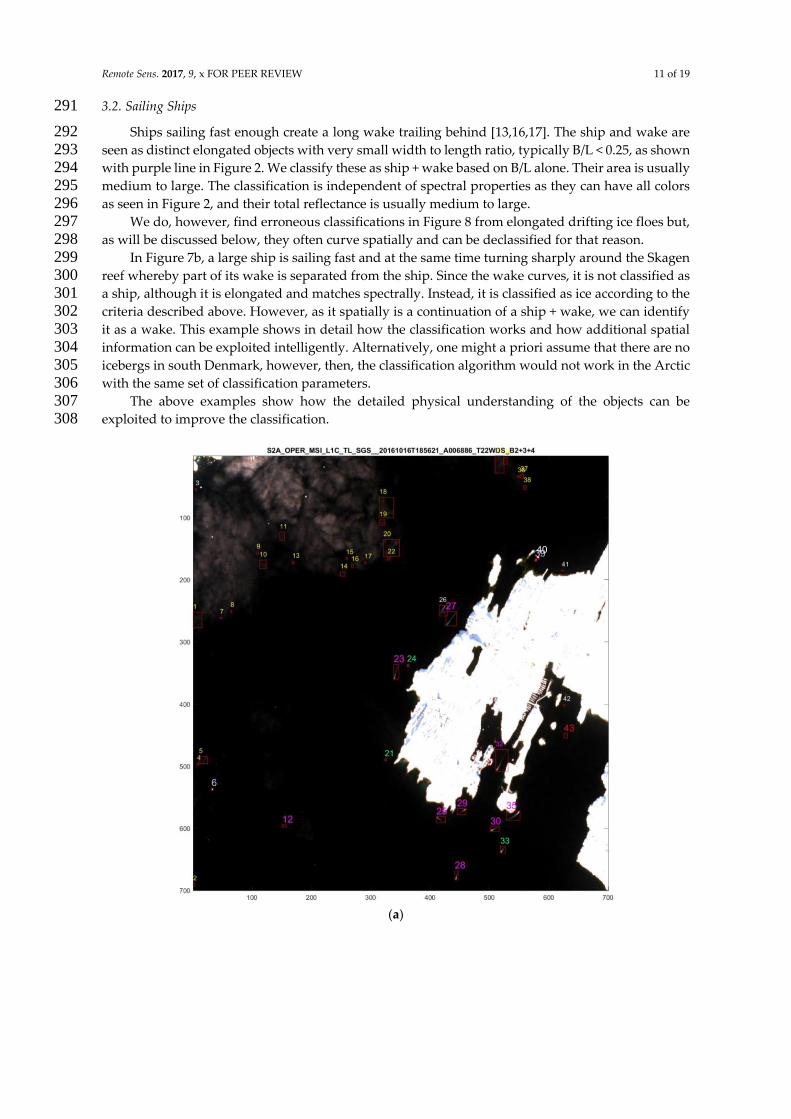
In Figure 7b, a large ship is sailing fast and at the same time turning sharply around the Skagen 299 reef whereby part of its wake is separated from the ship. Since the wake curves, it is not classified as 300 a ship, although it is elongated and matches spectrally. Instead, it is classified as ice according to the 301 criteria described above. However, as it spatially is a continuation of a ship + wake, we can identify 302 it as a wake. This example shows in detail how the classification works and how additional spatial 303 information can be exploited intelligently. Alternatively, one might a priori assume that there are no 304 icebergs in south Denmark, however, then, the classification algorithm would not work in the Arctic 305 with the same set of classification parameters. 306

The above examples show how the detailed physical understanding of the objects can be 307 exploited to improve the classification. 308

(a)


(b)

Figure 8. (a) Copernicus Sentinel-2A data as Figure 2 but from 16 October 2016, where snow has fallen. 309 The land is overexposed to see the clouds and grey ice appearing as patches in the sea northeast of 310 Nuuk. (b) Copernicus Sentinel-2 data but a week later, 23 October 2016. The grey ice abundance has 311 increased considerably. 312

3.3. Ships and Boats 313

Ships are elongated and we use the observed ratio B/L as a spatial classifier for ships. Spectrally, 314 we find that the ships have medium to large redness, generally such that smaller boats are green with 315 0.45 < RN < 0.6, whereas larger ships are red with RN > 0.6. This subdivision is not important for ship 316 classification but is practical since we anyway make this spectral subdivision for ice and islands for 317 larger ratio B/L as discussed below. 318

We also find that grey ice has a lower reflectance than most boats whereas icebergs have a higher 319 reflectance than boats. Therefore, the reflectance I4 can be used to discriminate and classify 320 these objects. 321

3.4. Islands 322

Islands come in all sizes and shapes but most have area larger than ships and shape less straight 323 and elongated than ships and therefore larger B/L. In addition, their temperatures are often larger 324 resulting in a redness above RN > 0.6, which is indicated by the red dashed line on the color bar of 325 Figure 4. 326

In Figures 7b and 10, a few large ships have fuel ship along side and therefore appear twice as 327 wide. These are on the border of being identified as islands. The discrimination parameter r = B0/L0 328 for the ratio of the ship breadth and width must therefore be chosen carefully. 329

As seen in Figures 2 and 8, several islands around Nuuk are correctly classified but a few are not 330 detected. If the islands are too close to land, their segment may not be separated from the land due 331


to ice floes clogging the narrow straight between them. In another case, two close-by islands cannot 332 be separated and are mis-classified as a long ship. These and other false positives and negatives can 333 be removed by adjusting the threshold for segment identification, however, at the cost of losing some 334 low reflectance objects close to the threshold. 335

3.5. Icebergs 336

Icebergs also come in all shapes and sizes. Spectrally, they are distinguished by having high 337 reflectance and being cold. On the redness scale, they are green 0.3 < RN < 0.45, as seen in Figure 9. A 338 number of icebergs are found and correctly classified in Figures 2 and 8. 339

Figure 9. Spatial and spectral scatter plots for Nuuk with abundant sea ice of Figure 8b. 340

3.6. Grey Ice 341

Ice comes in many forms, reflectivities and textures, and can be classified into subclasses such 342 as new ice, slush ice (nilas), young ice, grey ice, grey-white ice, first year ice, first year thin ice, second 343 year ice and multi-year ice. Eskimos have several dozens of different words for various types of ice 344 with and without layers of snow. Ice appears in increasing area and number during winter in the 345 Arctic particular in polar regions and in the ocean around Northeast Greenland, Jan Mayen and 346 Svalbard. Reflection and form vary with the age of the ice and underlying ocean currents. 347

As we are mainly interested in ships and icebergs, we classify all the above types of ice in one 348 class that simply will be referred to as “grey ice”. It appears as low intensity textures in the sea and 349 near the coast in the S2 winter images of Nuuk. Grey ice is not as highly reflecting (white) as icebergs 350 but can be as cold. 351

The grey ice may be thin and widespread and appear grey with low I4 as in the case of Figures 352 8.a+b. It is therefore advantageous in such cases to increase the threshold in order to reduce the 353 amount of sea ice objects and area. Instead other objects as icebergs, islands and ships appear which 354 otherwise would have been connected spatially with grey ice. 355

As mentioned above, we find that the convex area is a very useful spatial classifier for objects. 356 We find that ships and round objects such as some islands and icebergs have convex area about same 357 as the observed area, whereas ice floes and clouds often curve or have irregular surfaces. The 358 resulting larger convex area successfully discriminates in particular ice floes from ships. 359 Unfortunately, we also find exceptional cases where a fast and turning boat makes a curving wake 360 that therefore is mistakenly identified as an ice flow but these can be spatially correlated with nearby 361 ship + wakes. 362

363


3.7. Clouds 364

Clouds obscure the S2 imagery [13] depending on weather, geographical coordinates, time of 365 year, etc. For example, clouds cover Greenland about half of the time all year. Dense cloud cover 366 renders the imagery useless and even degrades S1 SAR imagery. Despite this, often the cloud cover 367 is only partial and is then useful to classify clouds. They come in all shapes and are generally white 368 with redness within 0.45 < NR < 0.6 and therefore difficult to discriminate from boats [10,11] and ice 369 floes. The S2 image in Figure 10 was selected because it contains a large number of smaller clouds, 370 which challenge the classification algorithm. By visual inspection, one can distinguish ships from 371 clouds from more complex texture features. We have thus far only included the spectral and spatial 372 classifiers as described above, but can foresee further improvements of our physical classification 373 algorithm embodying a number of more complex object texture features as for example described in 374 [10] or as widely employed in large area SAR imagery [2]. 375

Another way to discriminate clouds is through their infrared signature IR, which we find is 376 larger for clouds than surface objects such as boats and ice floes generally. We find that clouds 377 generally have IR > 0.45 and therefore use this classifier to separate them from ice floes, boats and 378 other objects that have IR < 0.45. 379

380

Figure 10. Copernicus Sentinel-2A data. Same as Figure 7b, but from 5 September 2016 at 10:30 a.m. 381 UTC, where a number of clouds are present. 382

3.8. Algal and Sea Clutter 383

Some sea clutter, algal blooming and sea current sediments are seen near the coast in Figures 1, 384 7 and 10. They only exceed the background threshold in a few cases, which are classified as grey 385


segments. For reasons of simplification, we ignore these few cases. In the future, we intend to extend 386 the classifications to include algal, oil spill, pollution, windmills, oil rigs and other objects in the sea. 387

4. Confusion Matrices, Classification Accuracy, False Positives and Negatives 388

For each of the S2 images, the classification algorithm results in a number of segments in each 389 class as described above. Each segment is subsequently identified as an object from a priori 390 knowledge of the images. For example, we know where the islands are situated, and that breaking 391 wakes are found along the coastline. Furthermore, we know that in the Skagen images the remaining 392 objects are mainly ships or clouds since there are no icebergs or grey ice. On the other hand, in the 393 Nuuk images, we can identify the few fishing boats as they all are sailing out of the harbor with long 394 ship wakes trailing behind. The remaining objects are islands, icebergs or grey ice. 395

Although this object classification is different for the Skagen and Nuuk images, the classification 396 algorithm is the same and with the same spectral and spatial classification parameters. The only 397 difference is the threshold and greyness parameters, which are larger in the Nuuk images because 398 the widespread ice floes have low reflectances. 399

In Table 1, we show the confusion matrix for all segments and objects in S2 images (Figures 1, 400 7.a+b and 10) of Skagen and in Table 2 those from images (Figures 2 and 8.a+b) of Nuuk. The segment 401 and object classification is described above. The classification parameters were chosen in order to 402 maximize the number of correct identifications in the diagonal. Off diagonal numbers are 403 mis-identifications or confused objects. False negatives lie above the diagonal and false positives 404 (false alarms) below. Concerning ships and icebergs, one prefers false positives rather than false 405 negatives in order not to miss any of these important objects. 406

Table 1. Confusion matrix for classifications from the Skagen area, Figures 1, 7.a+b, and 10. First 407 column lists the object classes and first row the segment classes (see text). Diagonal numbers are 408 correct identifications and non-diagonal numbers are mis-identified (confused) as false positives or 409 negatives. 410

Skagen Denmark Ship + Wake Ship Boat Island Icebergs Wake Grey Ice Cloud Total PA

Ship + Wake 25 0 0 0 0 0 0 0 25 1

Ships 0 18 0 0 1 0 0 0 19 0.93

Boats 0 0 61 5 0 0 16 8 90 0.68

Islands 0 0 0 2 0 0 0 0 2 1

Icebergs 0 0 0 0 0 0 0 0 0 -

Wakes 0 0 0 0 1 82 5 0 88 0.93

Grey ice 0 0 0 0 0 0 0 0 0 -

Clouds 0 0 0 2 0 6 0 173 181 0.96

Total 25 18 61 9 2 88 21 181 405

UA 1.0 1.0 1.0 0.22 0 0.93 0 0.96 0.89

Table 2. Confusion matrix as Table 1, but for the Nuuk area in Greenland, Figures 2 and 8.a+b. 411

Nuuk Greenland Ship + Wake Ship Boat Island Iceberg Wake Grey Ice Cloud Total PA

Ship + Wake 17 0 0 0 0 0 0 0 17 1.0

Ships 0 1 0 0 0 0 0 0 1 1.0

Boats 0 0 4 0 0 0 1 0 5 0.80

Islands 0 3 0 12 0 0 0 0 15 0.80

Icebergs 0 0 0 0 172 0 0 0 172 1.0

Wakes 0 0 0 0 1 0 0 0 1 0

Grey ice 0 0 21 0 0 3 20 3 47 0.43

Clouds 0 0 0 0 0 0 3 98 101 -

Total 17 4 25 12 173 3 24 101 359

UA 1.0 0.25 0.16 1 0.99 0 0.83 0.97 0.90

In Figure 10, there are a great number of clouds present. Spectrally, they appear in the yellow 412 class but most are not elongated spatially and can therefore be separated from boats. The infrared 413 classifier IR of Equation (7) is particular useful for correct cloud classification as can be seen in 414


Table 2. We validate the objects by visual inspection, since texture features distinguish the clouds 415 from ships. 416

In Table 1, the last column lists the object detection probability also called producer accuracy 417 (PA), i.e., the number of correct classification with respect to the total number detected of that object. 418 Only in few cases is an object not detected and therefore the number of objects present is almost the 419 same as the detection number. Last row lists the segment detection probability also called user 420 accuracy (UA). For all three Skagen images the overall accuracy is OA = 89%. Ship + wakes, ships and 421 boats are to a high degree classified correctly with PA = 100%, 93% and 68%, respectively, and UA 422 100%. Their performance factor F = 2 × PA × UA/(PA + UA) is F = 100%, 97% and 81% respectively. 423

We conclude that the classification algorithm is excellent for distinguishing ship + wakes, ships 424 and wakes. About 32% of the smaller boats are confused with grey objects and clouds. This is because 425 very small boats have low reflectance and may not be sufficiently elongated when they only extend 426 over few pixels. If we had a priori excluded ice around Skagen, we would have identified them 427 correctly as boats in these images. 428

In Table 2, we show the confusion matrix for Figures 2 and 8.a+b of the Nuuk area. Ship + wakes, 429 ships, islands, icebergs and clouds are correctly classified to a high degree. In Figure 8b, grey ice 430 appears in great numbers. Since the grey ice can appear in all forms and their number is large, a few 431 also fall in green elongated class and are mis-identified as boats resulting in a low UA = 16%. 432

It is not always possible by visual inspection to distinguish icebergs and grey ice, and it is likely 433 that some are confused. This is not cosnidered in Table 2. The confusion is not important as most 434 ships stay away from both. If icebreaker ships need to distinguish, our algorithm must be extended. 435 This would require ground truth information on positions of icebergs and sea ice in a given satellite 436 image. Ship + wakes are classified well, PA = 100%, but some cold islands are confused with ships. 437 The overall accuracy is OA = 90% 438

We learn from the supervised classification scheme applied to the Skagen and Nuuk images that 439 small boats are difficult to separate spatially and spectrally from grey ice, especially because we have 440 increased the grey ice parameter for the Nuuk images as compared to the Skagen images. The 441 important lesson learned is that it will be extremely difficult to find small boats in grey ice if they lie 442 still or are capsized. If they sail and create a wake, the boats and ships are easily detected and 443 accurately classified in Sentinel-2 images. 444

5. Conclusions 445

Several sets of S2 MSI satellite images over Skagen, the northernmost tip of Denmark, and Nuuk, 446 the capitol of Greenland, have been analyzed. Both contain a large number of ships and fishing boats 447 as well as wakes, islands, icebergs, sea ice and clouds. The search and segmentation model finds all 448 objects above a specified background. A supervised classification model was developed based on 449 spatial and spectral classification parameters that have direct physical meaning. Detailed information 450 on elongation, convex area, ship and wake correlations, allowed us to further improve and optimize 451 the classification model which resulted in fewer confusions. 452

The most important parameters (principal components) are the area and elongation for the 453 spatial part, and the total reflectivity, redness and infraredness for the spectral part. The first four 454 parameters are implicitly represented in the scatter plots of Figures 4 and 5 of all segments in Figure 455 1 from Skagen, Denmark, and likewise in Figure 9 from Nuuk, Greenland. 456

The optimal spectral and spatial classification parameters are the same for the satellite images 457 analysed here. The only scene dependent parameter is the threshold which was increased in the 458 complex Figure 8a,b to suppress the abundant sea-ice and cloud cover causing a number of false 459 alarm. The scene dependent parameter is a weakness of the model, and should be upgraded by some 460 automatic procedure. 461

Where large ships are very elongated, smaller boats fill fewer pixels and therefore generally less 462 elongated. The total reflectance is larger for icebergs, islands, and larger ships and their wakes, 463 whereas waves and small ships generally have smaller reflectance. Islands and large ships typically 464 have high redness, whereas icebergs, wakes and especially waves appear rather blue. Smaller ships 465


are more widely distributed between these limits and could be classified as boats if sufficiently 466 elongated. 467

The classification model proved very useful for detection and classification of sailing ships, 468 anchored ships, fishing boats, icebergs, grey ice, wakes, islands, and clouds. The resulting confusion 469 matrices display between 93% and 100% correct classifications of ships and icebergs in the less 470 complex S2 MSI satellite images without grey ice and clouds. However, the satellite images with 471 abundant sea ice or clouds were very challenging as these objects can come in a wide variation of 472 spatial and spectral forms, which led to a substantial increase in the number of false positives and 473 negatives as described in confusion matrices. 474

The classification model was trained and optimized on most of the data including the complex 475 images. Thus, validation on independent data was very limited. Consequently, the object 476 classification may be overfitted and the diagonalization of the confusion matrices optimistic. 477

These results can be compared to recent S1 SAR images regarding the ship classification 478 accuracy. A recent analysis of S1 Interferometric Wide Swath data [5] includes 27 SAR images 479 containing 7986 ships in total. The resolution is 10 m × 10 m and thus comparable to the S2 MSI. Their 480 optimal algorithm has a detection probability of 89% with 14% false detections, and a performance F 481 = 0.87. Their images do not contain sea ice (or clouds) and should therefore be compared to the 482 producer accuracy PA = 100% for ship + wakes and PA = 93% for ships in our multispectral S2 images. 483 In this comparison, we note that most of the boats in the multispectral images are smaller compared 484 to the 7986 ships analyzed in the SAR images. Furthermore, one should take into account that much 485 of S1 SAR data over the Arctic is in the Ground Range Detected either Extended Wide swath mode 486 with resolution 50 m × 50 m or Interferometric mode with resolution 20 m × 22 m, both considerably 487 worse than in Ref. [5]. Other satellites can provide better resolutions SAR and optical images in 488 narrower regions, but generally optical classification is considerably more accurate than SAR. 489

6. Outlook 490

An obvious extension of the object classification in marine and arctic environments from S2 MSI 491 is to include all 13 multispectral bands and to use pan- or hyper-sharpening techniques [26] for the 492 bands with lower resolution. Especially the infrared hyperspectral index IR was very useful for cloud 493 discrimination. 494

Another extension is with regard to spatial and texture classification by exploiting further details 495 of the spatial extent of the segments. For example, the curvature was useful for discriminating straight 496 ship wakes from ice floes, and such shape and texture properties may be further exploited. 497

Additionally, a comparison to Sentinel-1 SAR imagery with two polarizations will provide 498 complementary and weather-independent information although with substantial lower resolution 499 (except in the rare and narrow swath SM GRD full resolution mode). The synergy of S1 and S2 500 imagery should be investigated for daily searching and tracking of ships, icebergs and ice floes. 501

Acknowledgments: To ESA Copernicus for use of Sentinel-2 data around Nuuk and Skagen as shown in Figures 502 and described in Section 2. We thank H. Skriver and L. T. Pedersen for discussions on SAR data analysis. 503

Author Contributions: Peder Heiselberg performed the atmospheric corrections in sen2cor as well as pan-504 sharpening of all Sentinel-2 satellite images important for the infrared discrimination. Henning Heiselberg 505 developed and optimized the classification algorithm, validation and confusion matrices. 506

Conflicts of Interest: The authors declare no conflict of interest. 507

References 508

1. ESA Copernicus Program, Sentinel Scientific Data Hub. Available online: https://scihub.copernicus.eu 509 (accessed on 10 November 2017). 510

2. Zakhvatkina, N.; Korosov, A.; Muckenhuber, S.; Sandven, S.; Babiker, M. Operational algorithm for ice/water 511 classification on dual-polarized RADARSA2 images. Cryosphere Discuss. 2016, doi:10.5194/tc-2016-131. 512


3. Reid, T.; Walter, T.; Enge, P.J.; Fowler, A. Crowdsourcing Arctic Navigation Using Multispectral Ice 513 Classification & GNNS. In Proceedings of the 27th International Technical Meeting of the Satellite Division 514 of the Institute of Navigation, Tampa, FL, USA, 8–12 September 2014; pp. 707–721. 515

4. Brekke, C.; Weydahl, D.J.; Helleren, Ø.; Olsen, R. Ship traffic monitoring using multipolarisation satellite 516 SAR images combined with AIS reports. In Proceedings of the 7th European Conference on Synthetic 517 Aperture Radar (EUSAR), Friedrichshafen, Germany, 2–5 June 2008. 518

5. Kang, M.; Ji, K.; Leng, X.; Lin, A. Contextual Region-based Convolutional Neural Network with Multilayer 519 Fusion for SAR Ship Detection. Remote Sens. 2017, 9, 860, doi:10.3390/rs9080860. 520

6. Krogager, E.; Heiselberg, H.; Møller, J.G.; von Platen, S. Fusion of SAR and EO imagery for Arctic 521 surveillance. In Proceedings of the NATO IST-SET-128 Specialist Meeting, Norfolk, VA, USA, 4–5 May 2015. 522

7. Daniel, B.; Schaum, A.; Allman, E.; Leathers, R.; Downes, T. Automatic ship detection from commercial 523 multispectral satellite imagery. Proc. SPIE. 2013, 8743, doi:10.1117/12.2017762. 524

8. Burgess, D.W. Automatic ship detection in satellite multispectral imagery. Photogramm. Eng. Remote Sens. 525 1993, 59, 229–237. 526

9. Zhu, C.; Zhou, H.; Wang, R.; Guo, J. A novel hierarchical method of ship detection from spaceborne optical 527 image based on shape and texture features. IEEE Trans. Geosci. Remote Sens. 2010, 48, 3446–3456. 528

10. Corbane, C.; Marre, F.; Petit, M. Using SPOT-5 HRG data in panchromatic mode for operational detection 529 of small ships in tropical area. Sensors 2008, 8, 2959–2973. 530

11. Corbane, C.; Najman, L.; Pecoul, E.; Demagistri, L.; Petit, M. A complete processing chain for ship detection 531 using optical satellite imagery. Int. J. Remote Sens. 2010, 31, 5837–5854. 532

12. Tang, J.; Deng, C.; Huang, G.-B.; Zhao, B. Compressed-domain ship detection on spaceborne optical image 533 using deep neural network and extreme learning machine. IEEE Trans. Geosci. Remote Sens. 2015, 53, 534 1174–1185. 535

13. Heiselberg, H. A Direct and Fast Methodology for Ship Recognition in Sentinel-2 Multispectral Imagery. 536 Remote Sens. 2016, 8, 1033, doi:10.3390/rs8121033. 537

14. Wu, G.; de Leeuw, J.; Skidmore, A.K.; Liu, Y.; Prins, H.H.T. Performance of Landsat TM in ship 538 detection in turbid waters. Int. J. Appl. Earth Obs. Geoinf. 2009, 11, 54–61. 539

15. Bi, F.; Zhuang, Y.; Bian, M.; Zhang, Q. A Decision Mixture Model-Based Method for Inshore Ship Detection 540 Using High-Resolution Remote Sensing Imaging. Sensors 2017, 17, 470, doi:10.3390/s17071470. 541

16. Lapierre, F.D.; Borghgraef, A.; Vandewal, M. Statistical real-time model for performance prediction of ship 542 detection from microsatellite electro-optical imagers. EURASIP J. Adv. Signal Process. 2009, 2010, 1–15. 543

17. Bouma, H.; Dekker, R.J.; Schoemaker, R.M.; Mohamoud, A.A. Segmentation and Wake Removal of 544 Seafaring Vessels in Optical Satellite Images. Proc. SPIE. 2013, 8897, doi:10.1117/12.2029791. 545

18. Gade, M.; Hühnerfuss, H.; Korenowski, G. Marine Surface Films; Springer: Heidelberg, Germany, 2006. 546 19. Leifer, I.; Lehr, W.J.; Simecek-Beatty, D.; Bradley, E.; Clark, R.; Dennison, P.; Hu, Y.; Matheson, S.; Jones, 547

C.E.; Holt, B.; et al. State of the art satellite and airborne marine oil spill remote sensing: Application to the 548 BP Deepwater Horizon oil spill. Remote Sens. Environ. 2012, 124, 185–209, doi:10.1016/2012.03.024. 549

20. Lupidi, A.; Stagliano, D.; Martorella, M.; Berizzi, F. Fast Detection of Oil Spills and Ships Using SAR Images. 550 Remote Sens. 2017, 9, 230, doi:10.3390/rs9030230. 551

21. Immitzer, M.; Vuolo, F.; Atzberger, C. First experience with Sentinel-2 data for crop and tree species 552 classifcations in Central Europe. Remote Sens. 2016, 8, 166, doi:10.3390/rs8030166. 553

22. Ng, W.-T.; Rima, P.; Einzmann, K.; Immitzer, M.; Atzberger, C.; Eckert, S. Assessing the Potential of 554 Sentinel-2 and Pléiades Data for the Detection of Prosopis and Vachellia spp. in Kenya. Remote Sens. 2017, 9, 555 74, doi:10.3390/rs9010074. 556

23. Novelli, A.; Aguilar, M.A.; Aguilar, F.J.; Nemmaoui, A.; Tarantino, E. AssesSeg—A Command Line Tool to 557 Quantify Image Segmentation Quality: A Test Carried Out in Southern Spain from Satellite Imagery. 558 Remote Sens. 2017, 9, 40, doi:10.3390/rs9010040. 559

24. Müller-Wilm, U.; Louis, J.; Richter, R.; Gascon, F.; Niezette, M. Sentinel-2 level 2A prototype processor: 560 Architecture, algorithms and first results. In Proceedings of the ESA Living Planet Symposium, Edinburgh, 561 UK 9–13 September 2013; ESA SP-722, December 2013, Sen2cor Version 2.4.0. 562

25. Kaplan, G.; Avdan, U. Object-based water body extraction model using Sentinel-2 satellite imagery. Eur. J. 563 Remote Sens. 2017, 50, 137–143. 564

26. Selva, M.; Aiazzi, B.; Butera, F.; Chiarantini, L.; Baronti, S. Hyper-sharpening: A first approach on SIM-GA 565 data. IEEE J. Sel. Top. Appl. Earth Obs. Remote Sens. 2015, 8, 3008–3024. 566

https://doi.org/10.1016/j.rse.2012.03.024


© 2017 by the authors. Submitted for possible open access publication under the 567 terms and conditions of the Creative Commons Attribution (CC BY) license 568 (http://creativecommons.org/licenses/by/4.0/). 569

article ship-iceberg discrimination in sentinel-

Documents