article experimental study of the performance of a novel

Article 1

Experimental Study of the Performance of A Novel 2

Vertical Axis Wind Turbine 3

4

J. Agbormbai1 and W.D. Zhu2 5

6

1University of Maryland, Baltimore County,1000 Hilltop Circle, Baltimore, MD 21250;USA; 7

[email protected] 8

2University of Maryland, Baltimore County,1000 Hilltop Circle, Baltimore, MD 21250; USA; [email protected] 9

Correspondence: [email protected]; [email protected] 10

11

Abstract: The basic equation for estimating the aerodynamic power captured by an Anderson 12

Vertical Axis Wind Turbine (AVAWT) is a solution of the Navier-Stokes(N-S) equations 13

for a baroclinic, inviscid flow. In a nutshell, the pressure difference across the AVAWT is 14

derived from Bernoulli’s equation; an upshot of the integration of the N-S momentum 15

equation for a baroclinic inviscid flow, Euler’s momentum equation. The resulting 16

expression for the pressure difference across the AVAWT rotor is plotted as a function of 17

freestream speed. Experimentally determined airstream speeds at the AVAWT inlet and 18

outlet, coupled with corresponding freestream speeds are used in estimating the 19

aerodynamic power captured. The aerodynamic power is subsequently used in calculating 20

the aerodynamic power coefficient of the AVAWT. The actual power coefficient is calculated 21

from the power generated by the AVAWT at various free stream speeds and plotted as a 22

function of the latter. Experimental results show that, at all free stream speeds and tip speed 23

ratios, the aerodynamic power coefficient is higher than the actual power coefficient of the 24

AVAWT. Consequently, the power generated by the AVAWT prototype is lower than the 25

aerodynamic power captured, given the same inflow wind condition. 26

27

Keywords: Anderson-Vertical-Axis-Wind-Turbine, Actual-Power, Aerodynamic-Power, 28

Blockage-Factor, Power-Coefficient, Tip-speed-Ratio 29 30

31

Preprints (www.preprints.org) | NOT PEER-REVIEWED | Posted: 11 October 2019 doi:10.20944/preprints201910.0133.v1

© 2019 by the author(s). Distributed under a Creative Commons CC BY license.

mailto:[email protected]

mailto:[email protected]

https://doi.org/10.20944/preprints201910.0133.v1

http://creativecommons.org/licenses/by/4.0/

2 of 20

1. Introduction 32

Albeit vertical axis wind turbines are not new to subject matter experts, it is worthwhile shedding some light on 33

them so that, readers who are not subject matter experts can acquire some knowledge about these contrivances. 34

Besides the VAWT under investigation is a new contraption, something which makes an overview of existing 35

VAWTs relevant. In their bid to demonstrate the aerodynamic feasibility of a curved bladed Darrieus vertical 36

axis wind turbine (VAWT) rotor, engineers at the Sandia Laboratory of the US department of energy (USDOE) 37

developed a 5m diameter two bladed prototype which was mounted on the roof of their laboratory and observed 38

to rotate on windy days. Following the afore-mentioned rotor was the development of a 17m diameter curved, 39

two bladed rotor which was observed to perform nearly as efficiently as a horizontal axis wind turbine (HAWT) 40

rotor of equal capacity. A 34m diameter VAWT of same type, called the test rig by Sandia, was developed 41

thereafter and incorporated with instruments for condition monitoring and instruments to record weather 42

conditions that affect its performance. Sandia laboratory also uses this VAWT to; validate various computer 43

models, test airfoil designs and develop various control strategies [1]. Unlike this study that performs a wind 44

tunnel experiment to investigate the performance of a novel VAWT, the Sandia laboratory performs on-site 45

investigations on a working VAWT. 46

Typically, VAWTs may have either drag-driven or lift-driven rotors. The Savonius rotor is the most common 47

drag driven rotor. It has been used on water pumps and is cheap to manufacture. Savonius machines typically 48

have low power coefficients because of their being drag driven. Power coefficients of about 0.30 are typical of 49

Savonius rotors. Additionally, they have solidity close to unity, so-much-so that, they are very heavy relative to 50

their power production capacity and it is also difficult to protect them from high winds [2]. 51

The Darrieus VAWT is a lift-driven machine. Lift-Driven VAWTs have almost always been used for electrical 52

power generation. Lift-driven VAWTs typically have rotors with straight blades or curved blades. Some 53

VAWTs with straight blade rotors have a pitching mechanism, even though most lift driven VAWTs have fixed 54

blades. Yawing mechanisms are not needed on VAWTs, since they see the wind in any direction. The rotor 55

blades of lift driven VAWTs are generally untwisted and are of constant chord, thus, they are easy to 56

mass-produce. VAWTs are prone to high fatigue damage because, the load on each blade varies during each 57

rotation of the rotor. They are difficult to support on separate tall towers, since a large portion of the rotor tends 58

to be close to the ground in a region of low wind speed. This results in less productivity, compared to a HAWT 59

of the same capacity [2,3]. 60

In 1988, a 100m high, 60m diameter Darrieus VAWT was installed in Canada. The 60m diameter VAWT ran 61

for six years with 94% availability [2]. As stated earlier on, Darrieus VAWTs work on the principle of 62

aerodynamic lift (i.e. the wind pulls the rotor blades along). On the contrary the traditional Holland type 63

windmill operates on the principle of drag (i.e. the wind pushes a manmade barrier such as a rotor blade) [1]. 64

Typically, Darrieus VAWTs have power coefficients between 0.4 and 0.42 [4]. They are not self-starting; some 65

drag ought to be imposed on them for them to be able to be self-starting. The installation of cups or vanes on 66

Darrieus VAWTs, makes them capable of trapping the wind, thus causing them to self-start [1,3]. Using the 67

foregoing methods to self-start the Darrieus VAWT, results in larger blades, such that, these methods were 68

abandoned. 69

To encourage the development of wind energy technology in the United States, the Federal Government gave 70

incentives such as a tax credit of 1.80cents/KWh of wind energy produced. The USDOE set a goal in 2008, to 71

achieve a 20% contribution to grid power by wind energy sources by the year 2030 [1]. This is clear evidence of 72

the fact that, there is a niche for wind energy in the US energy market. 73



3 of 20

VAWTs can effectively be used in urban areas where turbulent and unsteady wind is typical [5,6]. They have 74

inherent superiority over HAWTs in severe wind conditions, because, the wind enters their rotors from about 75

any direction without yawing. A discrepancy factor of 2 typically exists between computational fluid dynamics 76

(CFD) and wind tunnel experiment results; since, the effect of finite blade length and spoke drag are not usually 77

considered in CFD analysis. The performance of a VAWT with a steady inflow condition is not a reflection of 78

the actual performance of a VAWT operating in an urban environment, an upshot of the fact that, the wind 79

fluctuates in an urban environment. The wind turbine’s performance depends on the cube of the speed of the 80

inflow wind, thus, moderate fluctuations in wind speed would result in very large fluctuations in power [5]. The 81

seeming stagnation in improvements on the aerodynamics of HAWTs has spurred up interest in the 82

development of large scale VAWTs. Another factor in favor of VAWTs is the future demand for decentralized 83

and sustainable energy supply in Cities and rural communities [7]. They are suitable where HAWTs do not 84

operate efficiently, usually in locations with high wind speeds and turbulent wind flow. VAWTs are quieter 85

than HAWTs, something which makes them suitable for use in urban areas [8,9]. 86

Savonius VAWTs can withstand gusts because of their superior stalling behavior and are suitable for use in 87

gusty environments. At a tip speed ratio of unity, the power coefficient of a Savonius rotor is maximum. 88

Modifications on the blade geometry of Savonius rotors improve the power coefficient. The power coefficient 89

of a Savonius rotor with a 45º angle of twist is 0.3385 compared to the 0.30 for rotors with untwisted blades. 90

Two stage Savonius rotors perform better than their three stage counterparts. Both three bladed and two bladed 91

Savonius rotors exhibit high power coefficients at low tip speed ratios [8]. 92

Curved Darrieus VAWTs with troposkein shapes are prone to nearly tensile loads and minimal bending 93

moments on the rotor blades. They operate at distinct angles of attack at different azimuth angles and are 94

subjected to cyclic aerodynamic loads which can result in fatigue [9]. Cognizant of the afore-mentioned setback 95

on the curved Darrieus VAWTs and other VAWTs, the conduction of experiments and simulations in order to 96

ascertain their suitability for use is imperative. The International Electro-Technical Commission (IEC) 97

guidelines include well established procedures for wind turbine testing. Based on IEC guidelines, the service 98

life of Wind Turbines (WT) is 20 years. Breakdown times are frequent with WTs and such breakdown stem 99

from manufacturing errors and design errors due to underestimated fatigue load or extreme loads. Consideration 100

of turbulent inflow conditions during aerodynamic modelling is of paramount importance. The turbulent 101

characteristics of the inflow air may have an impact on the fatigue loads experienced by the WT [10]. 102

Blade pitching is more difficult for VAWTs than for HAWTs because of the dependence of the angle of attack 103

of the former on the rotor azimuth angle; resulting in the existence of very few practical pitch control schemes 104

for VAWTs [11]. Unlike some of the existing VAWTs which may require pitch control to maximize wind 105

energy capture, the VAWT in this study does not require pitch control for wind energy capture optimization. 106

The extraction of the wind’s momentum by the VAWT occurs more during the upwind pass. Most of the 107

VAWT’s power output is produced on the upwind pass whereas flow momentum is considerably reduced on the 108

downwind pass, hence resulting in a reduced power output [12]. Darrieus type VAWTs with straight blades are 109

less efficient than those with helically twisted blades [13]. 110

Various numerical and analytical schemes have been implemented in a bid to investigating the performance 111

characteristics of VAWTs. Zanon et al [14] solved potential flow equations in conjunction with integral 112

boundary layer equations formulated for the VAWT rotor, using a semi-inverse iterative algorithm. From their 113

simulations they inferred that, VAWTs can be designed to avoid the occurrence of dynamic stall resulting from 114

blade-vortex interaction in the downward part of rotor rotation during gusts, normal operation and even at low 115

tip speed ratios [14].Scheurich and others [13] implemented a Computational Fluid Dynamics (CFD) scheme 116



4 of 20

based on the vortex transport model (VTM). The VTM is based on solving the Navier-Stokes(N-S) equations in 117

terms of vorticity and velocity. The governing momentum equation is expressed in terms of vorticity and 118

velocity and is the result of finding the curl of the velocity and pressure-based N-S momentum equation. In 119

their work on the steady state and dynamic simulations of Savonius rotors, Jaohindy et al [15], found out that, 120

the best approximations of the static torque coefficient, the dynamic torque coefficient and the power 121

coefficient were obtained using the shear stress transport (SST)-k- rather than k- turbulence models. At 122

startup, the dynamic torque coefficient curves of a Savonius rotor oscillate around fixed values in polar 123

coordinates [15].There is a significant difference between the simulated and experimental values of the power 124

coefficient of a Darrieus VAWT at high tip speed ratios even though simulation and experimental power 125

coefficient values follow the same trend as the tip speed ratio varies [16]. The power coefficient of a Darrieus 126

type VAWT peaks at tip speed ratios between 3 and 4 and drops for tip speed ratios greater than 4 for both CFD 127

simulation results and experimental results with values of the former being slightly higher than those of the 128

latter (See figure 18 of reference [17]). 129

This study uses an experimental approach to investigate the performance of a novel VAWT. Unlike the CFD 130

simulations performed by some of the cited authors, which were based on two or three tip speed ratios, this 131

study investigates the performance characteristics of the novel VAWT over a broad range of tip speed ratios. 132

The VAWT under investigation is a novel VAWT invented and patented by Bruce E. Anderson, under patent 133

number US8790069. 134

2.0 Basic Equations of Fluid Dynamics 135

Stating without proof; for baroclinic flows the integral of the Navier-Stokes equation [18,19,20] results in the 136

Bernoulli’s equation given by; 137

21

| |2

pV gz

M , (1) 138

For one dimensional (1-D) baroclinic flows, V U and p p

, yielding; 139

21

2gz

pU

M , (2) 140

Applying eqn. (2) to stations 0-1 in Fig. 1, we have; 141

2 20 10 1

1 1

2 2gz gz

p pU U

which on further simplifying, yields,

2 20 10 1

1 1

2 2

p pU U

and 142

2 2010 1

1 1

2 2

ppU U

, (3) 143

Applying eqn. (2) to stations 2-3 in fig. 1 below we have; 2 2 022 3

1 1

2 2gz gz

ppU U

, which on 144

simplifying further, yields, 2 2 022 3

1 1

2 2

ppU U

and 145



5 of 20

146

Figure.1 Control Volume of the Anderson VAWT 147

2 20 22 3

1 1

2 2

p pU U

, (4) 148

Adding eqn. (3) to eqn. (4) yields; 149

2 2 2 21 20 1 2 3

1 1 1 1

2 2 2 2

p pU U U U

. (5) 150

Applying eqn. (2) to stations 1-2 in fig. 1 below we have; 2 21 2

1 2

1 1

2 2gz gz

p pU U

, which on 151

simplifying further, yields, 2 21 2

1 2

1 1

2 2

p pU U

and 152

153

2 21 22 1

1 1

2 2

p pU U

, (6) 154

Adding eqns. (5) and (6) yields; 155

2 2 2 21 20 1 2 3

1 1

2 22( )

p pU U U U

, (7) 156



6 of 20

Momentum is recovered far downwind the VAWT, because of the atmospheric boundary layer, thus, 157

3 0U U and equation (7) becomes; 2 21 2

2 1

1 1

2 2

p pU U

, which on simplifying further yields the 158

pressure drop across the VAWT below; 159

2 2

2 1 1 2

1

2( )p p U U , (8) 160

The wind power captured could be calculated from the rate of change of kinetic energy as follows: 161

2 2

0 2

1( )

2Power m U U , (9) 162

But 1m AU and equation (9) becomes, 163

2 2

1 0 2

1( )

2Power AU U U , (10) 164

The total energy borne by the wind seen by the VAWT is given by, 165

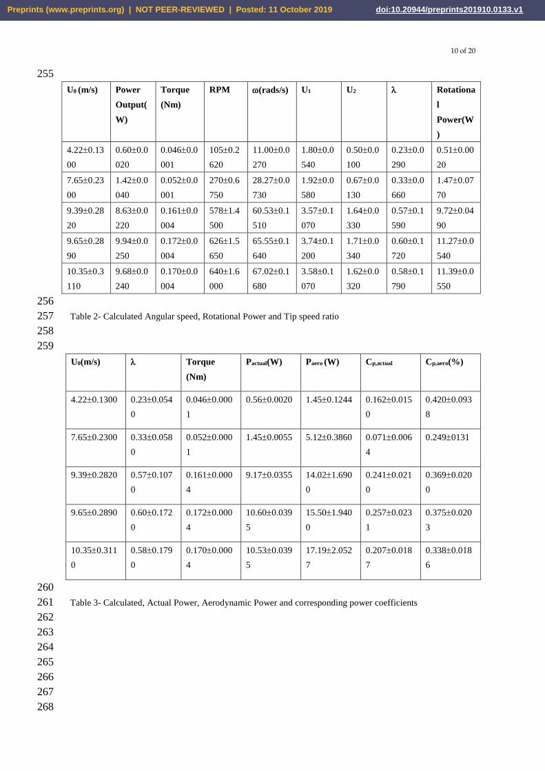
3

max 0

1

2P AU , (11) 166

The power coefficient, Cp, is given by; 167

max/pC P P , (12) 168

169

4.0 Aim of the Experiment 170

The purpose of this experiment is multipronged, namely, to prove that the Anderson Vertical Axis Wind 171

Turbine (AVAT) can generate electricity, to determine the power coefficient of an AVAWT, to investigate its 172

dependence on free stream speed and the tip speed ratio and to investigate the dependence on free stream speed 173

and tip speed ratio of the torque and the power generated. 174

5.0 Experimental Procedures 175

The International Electro-Technical Committee’s (IEC) standard number: IEC61400-12-1, requires that, on-site 176

measurements of electric power generated by wind turbines be made at respective wind speeds. Based on the 177

afore mentioned, the power generated by the AVAWT model is measured at respective free stream speeds. It is 178

worthwhile noting that, the apparatus used in this experiment consists of a 55.88cm x 60.96cm x182.88cm 179

custom made plywood wind tunnel, a 17.78cm diameter x 41.91cm high AVAWT model, a Benetech hotwire 180

anemometer (Model: GM 8903 with a resolution of 0.1 /m s and a memory of 350 records), a Hylec MS 181

6252 digital anemometer( with a resolution of 0.01 /m s ), a Torquesense model RWT421-DD-KG torque 182

transducer with a maximum torque range of 17.5Nm, a steel rule, a try square, a Lenovo Ideapad P400 Touch 183

laptop computer and a Canon PowerShot A570IS digital camera. The torque transducer measures torque, power 184

output and rotational frequency in RPM. 185

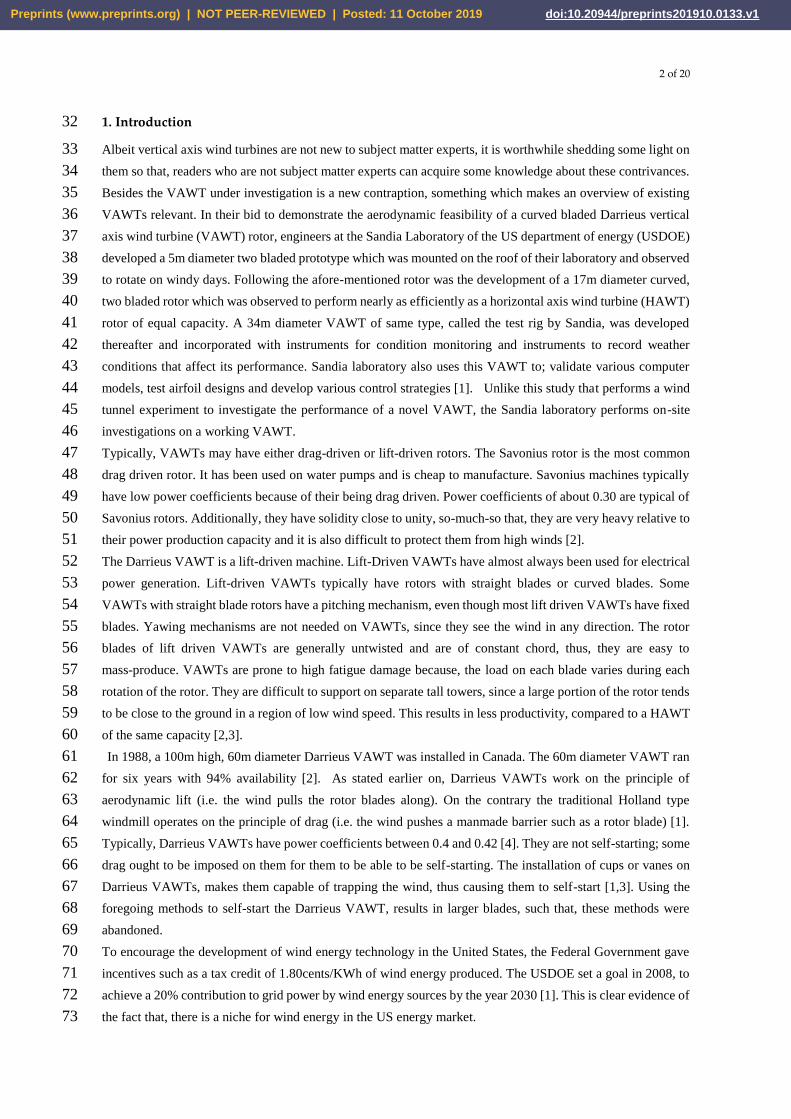
Prior to carrying out the experiment, the setting of the fan used on the wind turbine was calibrated by measuring 186

the speed of air (free stream speed) at the center of the wind tunnel with the AVAWT model not in place, using 187

a hot wire anemometer as shown in plate 1 below. The free stream speed was measured for each of the twelve 188

settings on the fan motor’s variable speed drive. All observations were recorded. Experiments were carried out 189

after the necessary safety precautions were followed. All view windows were firmly short, the fan end of the 190



7 of 20

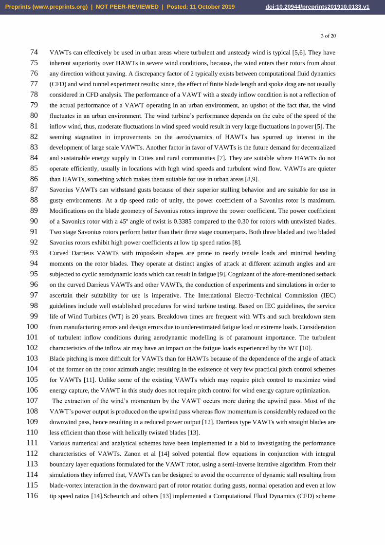
wind tunnel was provided with a protective wire gauze screen to prevent users from being injured by rotating 191

equipment. Plate 2 and Figure 2 below depict the setup of the experiment. 192

193

194

Plate 1- Setup for the Calibration of the fan setting terms speed (m/s) 195

196

197

198

Plate 2- Setup for measuring VAWT performance parameters 199

The AVAWT model was installed in the wind tunnel as shown in plate 2 and Figure 2 and coupled to the torque 200

transducer. The hotwire anemometer was placed at a distance one rotor diameter upstream the AVAWT 201

strategically located to measure the wind speed at the center of the wind tunnel while the digital anemometer 202

was placed two rotor diameters downstream the AVAWT. All leads from measuring instruments to the laptop 203

were connected and the setup was put on by selecting the fan speed and turning on the fan motor. All readings 204

were taken and tabulated. 205



8 of 20

206

207

Figure 2- Experimental Setup showing Measurements. 208

5.1 Observations 209

It is worth noting that, the fan used in this experiment has 12 speed settings; seven of the speed setting lie 210

between 1.77m/s and 3.3m/s. These speed settings imparted no rotation on the AVAWT, so their results were 211

discarded. The recorded measurements of respective parameters at respective free stream speeds are shown in 212

table 1 below. Table 4 contains the estimated induction factors at the AVAWT inlet and outlet respectively. 213

5.2 Precision 214

Torque transducer measurements are within a margin of accuracy of 0 . 2 5 % . The hotwire anemometer 215

measurements are within a margin of accuracy of 3.0% , while the digital anemometer readings are within a 216

margin of accuracy of 2.0% . 217

218

219

5.3 Calculations 220

The angular speed of the AVAWT is calculated from the measured RPM using eqn. (13) below: 221

2

60

RPM , (13) 222

The rotational power is calculated from the angular speed and the measured torque, T, as follows; 223

rotP T , (14) 224

actualP , the average power is reckoned from the measured electrical power and the rotational power using eqn. 225

(15) below; 226

2

rotactual

P PP

, (15) 227

aeroP , the aerodynamic power is given by eqn. (10) above as follows; 228

2 2

1 0 2

1( )

2aeroP AU U U , (16) 229



9 of 20

The respective power coefficients are estimated from eqn. (17) as follows: 230

, max/p actaul actualC P P , (17a) 231

, max/p aero aeroC P P , (17b) 232

The tip speed ratio is given by eqn. (18) below; 233

0

R

U

, (18) 234

Where R is the radius of the AVAWT rotor. The induction factor at the AVAWT inlet, a is given by; 235

0 1

0

U Ua

U

, (19a) 236

The average induction factor a is given by; 237

(1/ 5) aa , (19b) 238

The multiplication factor on the induction factor at the AVAWT exit, m is given by; 239

20

0

U Um

aU

, (20a) 240

(1/ 5) mm , (20b) 241

242

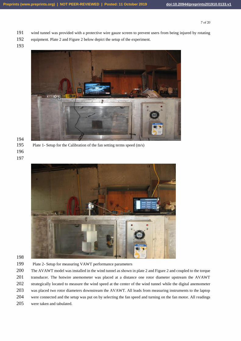
6.0 Results and Discussion 243

Experimental data are used to estimate the parameters expressed in eqns. (8) through (20b) and tabulated as 244

shown in tables 2, 3 and 4 below. Figures 3 to 10 below depict graphs plotted from experimental results. The 245

average induction factor, a , calculated from experimental measurements of the upwind and downwind free 246

stream speeds using Eqns. (19a and b) is 0.642 0.876 and the downwind speed could be expressed as 247

2 0 (1 )U U ma . Where m is an average value estimated from measured upwind and downwind speeds 248

using Eqns. (20a and b) and is 1.34 0.1122 . Thus, the AVAWT rotor inlet and outlet air speeds are given 249

as follows; 250

251

U0 (m/s) Power

Output(W)

Torque

(Nm)

RPM

4.220.1300 0.600.0020 0.0460.0001 1050.2620

7.650.2300 1.420.0040 0.0520.0001 2700.6750

9.390.2820 8.630.220 0.1610.0004 5781.4500

9.650.2890 9.940.0250 0.1720.0004 6261.5650

10.350.3110 9.680.0240 0.1700.004 6401.6000

252

Table 1-Experimental Data 253

254



10 of 20

255

U0 (m/s) Power

Output(

W)

Torque

(Nm)

RPM (rads/s) U1 U2 Rotationa

l

Power(W

)

4.220.13

00

0.600.0

020

0.0460.0

001

1050.2

620

11.000.0

270

1.800.0

540

0.500.0

100

0.230.0

290

0.510.00

20

7.650.23

00

1.420.0

040

0.0520.0

001

2700.6

750

28.270.0

730

1.920.0

580

0.670.0

130

0.330.0

660

1.470.07

70

9.390.28

20

8.630.0

220

0.1610.0

004

5781.4

500

60.530.1

510

3.570.1

070

1.640.0

330

0.570.1

590

9.720.04

90

9.650.28

90

9.940.0

250

0.1720.0

004

6261.5

650

65.550.1

640

3.740.1

200

1.710.0

340

0.600.1

720

11.270.0

540

10.350.3

110

9.680.0

240

0.1700.0

004

6401.6

000

67.020.1

680

3.580.1

070

1.620.0

320

0.580.1

790

11.390.0

550

256

Table 2- Calculated Angular speed, Rotational Power and Tip speed ratio 257

258

259

U0(m/s) Torque

(Nm)

Pactual(W) Paero (W) Cp,actual Cp,aero(%)

4.220.1300 0.230.054

0

0.0460.000

1

0.560.0020 1.450.1244 0.1620.015

0

0.4200.093

8

7.650.2300 0.330.058

0

0.0520.000

1

1.450.0055 5.120.3860 0.0710.006

4

0.2490131

9.390.2820 0.570.107

0

0.1610.000

4

9.170.0355 14.021.690

0

0.2410.021

0

0.3690.020

0

9.650.2890 0.600.172

0

0.1720.000

4

10.600.039

5

15.501.940

0

0.2570.023

1

0.3750.020

3

10.350.311

0

0.580.179

0

0.1700.000

4

10.530.039

5

17.192.052

7

0.2070.018

7

0.3380.018

6

260

Table 3- Calculated, Actual Power, Aerodynamic Power and corresponding power coefficients 261

262

263

264

265

266

267

268



11 of 20

U0 (m/s) a m

4.220.1300 0.5730.0540 1.540.0640

7.650.2300 0.7490.0580 1.220.0710

9.390.2820 0.6200.1070 1.330.1410

9.650.2890 0.6120.1120 1.340.1460

10.350.3110 0.654.01070 1.290.1390

269

Table 4- Estimates of Induction Factor 270

1 0 (1 )U U a , (21) 271

2 0 (1 (1.34 0.1122) )U U a , (22) 272

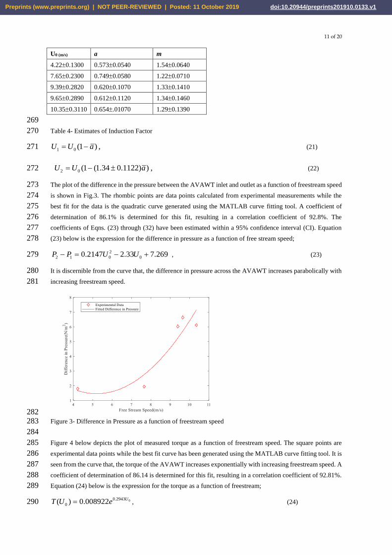
The plot of the difference in the pressure between the AVAWT inlet and outlet as a function of freestream speed 273

is shown in Fig.3. The rhombic points are data points calculated from experimental measurements while the 274

best fit for the data is the quadratic curve generated using the MATLAB curve fitting tool. A coefficient of 275

determination of 86.1% is determined for this fit, resulting in a correlation coefficient of 92.8%. The 276

coefficients of Eqns. (23) through (32) have been estimated within a 95% confidence interval (CI). Equation 277

(23) below is the expression for the difference in pressure as a function of free stream speed; 278

2

2 1 0 00.2147 2.33 7.269P P U U , (23) 279

It is discernible from the curve that, the difference in pressure across the AVAWT increases parabolically with 280

increasing freestream speed. 281

282

Figure 3- Difference in Pressure as a function of freestream speed 283

284

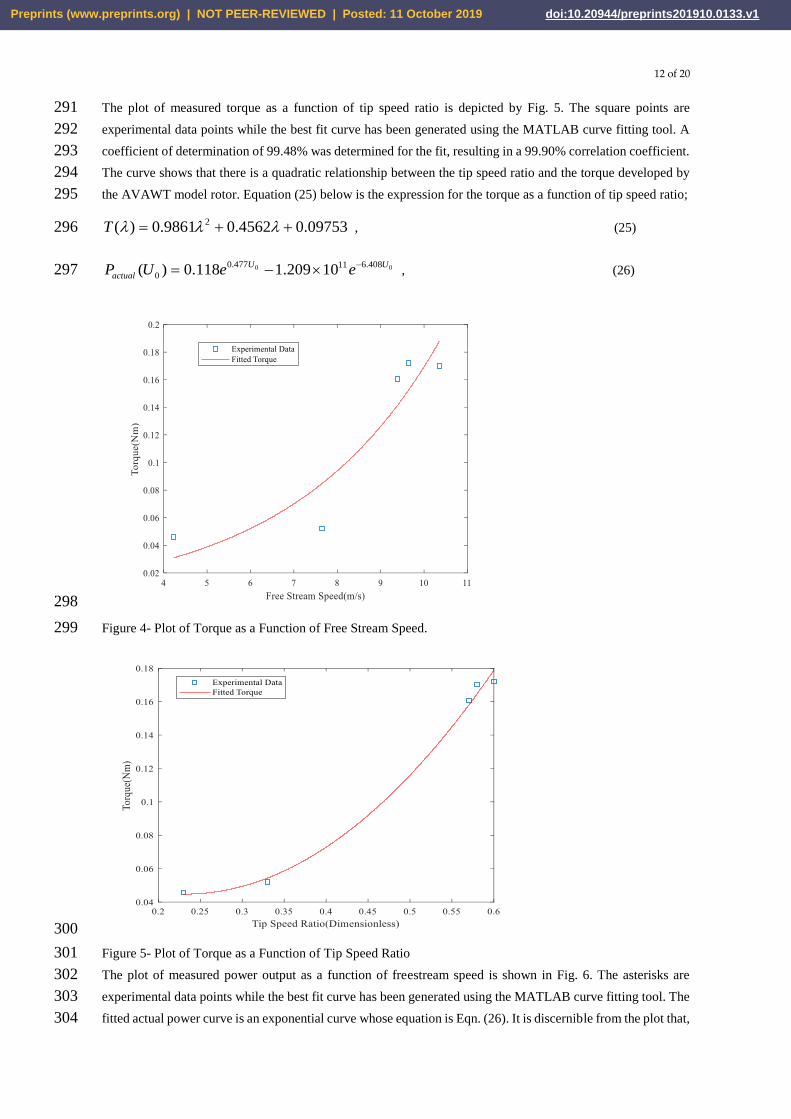
Figure 4 below depicts the plot of measured torque as a function of freestream speed. The square points are 285

experimental data points while the best fit curve has been generated using the MATLAB curve fitting tool. It is 286

seen from the curve that, the torque of the AVAWT increases exponentially with increasing freestream speed. A 287

coefficient of determination of 86.14 is determined for this fit, resulting in a correlation coefficient of 92.81%. 288

Equation (24) below is the expression for the torque as a function of freestream; 289

00.2943

0( ) 0.008922U

T U e , (24) 290



12 of 20

The plot of measured torque as a function of tip speed ratio is depicted by Fig. 5. The square points are 291

experimental data points while the best fit curve has been generated using the MATLAB curve fitting tool. A 292

coefficient of determination of 99.48% was determined for the fit, resulting in a 99.90% correlation coefficient. 293

The curve shows that there is a quadratic relationship between the tip speed ratio and the torque developed by 294

the AVAWT model rotor. Equation (25) below is the expression for the torque as a function of tip speed ratio; 295

2( ) 0.9861 0.4562 0.09753T , (25) 296

0 00.477 6.40811

0( ) 0.118 1.209 10U U

actualP U e e

, (26) 297

298

Figure 4- Plot of Torque as a Function of Free Stream Speed. 299

300

Figure 5- Plot of Torque as a Function of Tip Speed Ratio 301

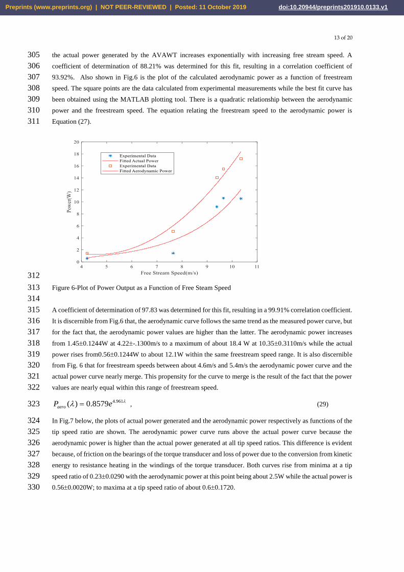
The plot of measured power output as a function of freestream speed is shown in Fig. 6. The asterisks are 302

experimental data points while the best fit curve has been generated using the MATLAB curve fitting tool. The 303

fitted actual power curve is an exponential curve whose equation is Eqn. (26). It is discernible from the plot that, 304



13 of 20

the actual power generated by the AVAWT increases exponentially with increasing free stream speed. A 305

coefficient of determination of 88.21% was determined for this fit, resulting in a correlation coefficient of 306

93.92%. Also shown in Fig.6 is the plot of the calculated aerodynamic power as a function of freestream 307

speed. The square points are the data calculated from experimental measurements while the best fit curve has 308

been obtained using the MATLAB plotting tool. There is a quadratic relationship between the aerodynamic 309

power and the freestream speed. The equation relating the freestream speed to the aerodynamic power is 310

Equation (27). 311

312

Figure 6-Plot of Power Output as a Function of Free Steam Speed 313

314

A coefficient of determination of 97.83 was determined for this fit, resulting in a 99.91% correlation coefficient. 315

It is discernible from Fig.6 that, the aerodynamic curve follows the same trend as the measured power curve, but 316

for the fact that, the aerodynamic power values are higher than the latter. The aerodynamic power increases 317

from 1.450.1244W at 4.22-.1300m/s to a maximum of about 18.4 W at 10.350.3110m/s while the actual 318

power rises from0.560.1244W to about 12.1W within the same freestream speed range. It is also discernible 319

from Fig. 6 that for freestream speeds between about 4.6m/s and 5.4m/s the aerodynamic power curve and the 320

actual power curve nearly merge. This propensity for the curve to merge is the result of the fact that the power 321

values are nearly equal within this range of freestream speed. 322

4.961( ) 0.8579aeroP e , (29) 323

In Fig.7 below, the plots of actual power generated and the aerodynamic power respectively as functions of the 324

tip speed ratio are shown. The aerodynamic power curve runs above the actual power curve because the 325

aerodynamic power is higher than the actual power generated at all tip speed ratios. This difference is evident 326

because, of friction on the bearings of the torque transducer and loss of power due to the conversion from kinetic 327

energy to resistance heating in the windings of the torque transducer. Both curves rise from minima at a tip 328

speed ratio of 0.230.0290 with the aerodynamic power at this point being about 2.5W while the actual power is 329

0.560.0020W; to maxima at a tip speed ratio of about 0.60.1720. 330



14 of 20

331

Figure 7- Plot of Power Output as a function of Tip speed ratio 332

At a tip speed ratio of 0.60.1720, the actual power read from the graph is about 10.9W while the aerodynamic 333

power is about16.8W. The best fit for the actual power as a function of tip speed ratio determined with the 334

MATLAB plotting tool is a quadratic polynomial as expressed in Eqn. (28). A coefficient of determination of 335

99.44% was determined for this fit, resulting in a correlation coefficient of 99.71%. An exponential curve is the 336

best fit for plot of aerodynamic power as a function of tip speed ratio, . The relationship between the tip 337

speed ratio and the aerodynamic power is expressed in Eqn. (29). A coefficient of determination of 95.94% was 338

determined for this fit using the MATLAB plotting tool, resulting in a correlation coefficient of 97.95%. It is 339

discernible from the plot that the aerodynamic power values are higher than the actual power generated. This 340

difference in power is the result of the fact that, the aerodynamic power is derived from the rate of loss of kinetic 341

energy by the airstream; something which does not account for the friction losses on the torque transducer 342

bearings. 343

344

345

Figure 8- Power Coefficient as a Function of Freestream speed 346

347



15 of 20

Figure 8 depicts the plot of power coefficient as a function of free stream speed. The curve of actual power 348

coefficient is below the curve of the aerodynamic power coefficient. There is a scatter between the experimental 349

data and the fitted curve of actual power coefficient; same is true for the aerodynamic power coefficient. Both 350

curves are parabolas with upward concavity, thus implying that both the aerodynamic and actual power 351

coefficients vary quadratically with varying freestream speed. The curve of the actual power coefficient has a 352

minimum value of about 0.1 at a freestream speed of about 6.5m/s while the curve of the aerodynamic power 353

coefficient has a minimum value of about 0.28 at a freestream speed of about 7.3m/s. It is discernible from the 354

graphs that, the aerodynamic power coefficient is higher than the actual power coefficient at all free stream 355

speeds. This difference in power coefficient results from power losses due to drag, friction on bearings and 356

losses in the generator windings. Equations (30) and (31) below express the relationship between the actual 357

power coefficient, the aerodynamic power coefficient respectively and the free stream speed. A coefficient of 358

determination of 56.25% was determined for Eqn. (30), using the MATLAB plotting tool; resulting 359

in a correlation coefficient of 75. The coefficient of determination determined for Eqn. (31) is 61.73%, 360

yielding a correlation coefficient of 78.57%. 361

2

, 0 0 0( ) 0.0198 0.1396 0.552p actualC U U U , (30) 362

2

, 0 0 0( ) 0.01206 0.1808 0.9629p aeroC U U U , (31) 363

364

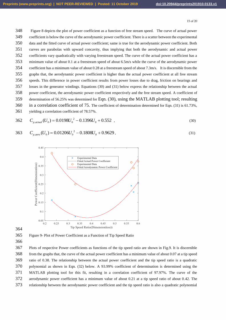
Figure 9- Plot of Power Coefficient as a Function of Tip Speed Ratio 365

366

Plots of respective Power coefficients as functions of the tip speed ratio are shown in Fig.9. It is discernible 367

from the graphs that, the curve of the actual power coefficient has a minimum value of about 0.07 at a tip speed 368

ratio of 0.38. The relationship between the actual power coefficient and the tip speed ratio is a quadratic 369

polynomial as shown in Eqn. (32) below. A 93.99% coefficient of determination is determined using the 370

MATLAB plotting tool for this fit, resulting in a correlation coefficient of 97.97%. The curve of the 371

aerodynamic power coefficient has a minimum value of about 0.21 at a tip speed ratio of about 0.42. The 372

relationship between the aerodynamic power coefficient and the tip speed ratio is also a quadratic polynomial 373



16 of 20

given by Eqn. (33). A coefficient of determination of 89.67% is determined using the MATLAB plotting tool 374

for this fit, resulting in a correlation coefficient of 94.67%. 375

2

, ( ) 4 .095 3.121 0.6603p a c t u a lC , (32) 376

2

, ( ) 5 .573 4 .694 1 .2p a e r oC , (33) 377

It is discernible from Fig. 9 that, the aerodynamic power coefficient curve runs above the actual power 378

coefficient curve. This is because, the aerodynamic power coefficient is higher than the actual power coefficient 379

within the entire range of the tip speed ratios. The aerodynamic power coefficient is an indicator of the rate of 380

change of kinetic energy as the air passes through the AVAWT while the actual power coefficient indicates the 381

rate of energy conversion to electricity as the air flows past the AVAWT. It is worth noting that the best way to 382

determine the power coefficient of a wind turbine (WT) is by measuring the actual power generated by the WT. 383

The use of aerodynamic parameters to determine the power coefficient, results in higher values even when no 384

power is generated. 385

Based on the results of the experiment, the average power coefficient due to the actual power generated by 386

the AVAWT is 0.1880.0168 while the average aerodynamic power coefficient of the AVAWT model rotor is 387

about 0.3500.0332, the power coefficient of a Savonius rotor is 0.30[3], the power coefficient of the Darrieus 388

VAWT is between 0.4 and 0.42[4] and the power coefficient of a modified Savonius rotor with a 45° angle of 389

twist is 0.3385[8]. It is worth noting that, unlike Darrieus type VAWTs that are not self-starting, the AVAWT is 390

self-starting. 391

392

7.0 Wall Effects of the Wind Tunnel 393

Wind tunnel wall effects have an impact on the drag coefficient (CD) and hence the drag on a model being 394

tested in it. Damljanovic and others [21] discovered that for blockage ratios ranging from 0.5% to 0.6% and 395

angles of attack within 10 , wind tunnel wall effects are negligible within measurement uncertainties. Other 396

workers [22] performed numerical simulations on models with blockage ratios of 1.875% and 15% respectively 397

and arrived at the conclusion that, the drag coefficient increased with increasing blockage ratio. Per these 398

workers, it is reasonable to use the method of images in studying the wall effects of a wind tunnel on the drag 399

experienced by a model being tested. In this study, the method of images is used to study the effects of the wind 400

tunnel walls on the drag on the AVAWT model. 401

Awbi et al [23] working with a spherical model, discovered that, the drag coefficient did not vary with Reynolds 402

number (Re) for Re ranging from 6.5x 104 to 2.2x 105, but it increased with increasing blockage ratio. This 403

increase in drag coefficient is lower for critical values of Re than for less than critical Re. The increase in drag 404

coefficient is lower for critical Re because the wake is narrower, resulting in a lower wake blockage effect. The 405

method of images for blockage correction, splits wind tunnel wall effects into solid blockage ( s ) due to the 406

physical dimensions of the model and wake blockage ( w ) due to the wake. Summing the two blockage factors 407

yields the overall blockage factor ( ), where; 408

s w , (34) 409

The net effect of the wind tunnel wall is the sum of the induced speed and the wind tunnel free stream speed as 410

expressed in eqn. (35) below [23]: 411



17 of 20

0 (1 )U U , (35) 412

For the AVAWT model, the effect of blockage is to reduce the wind tunnel velocity, since the rotor rotates with 413

energy extracted from the air that flows past it. Thus, eqn. (35) becomes; 414

0 (1 )U U , (36) 415

After some algebraic manipulations on A. Thom’s formula [23], the drag coefficient is given in terms of w 416

and the blockage ratio, br , as follows: 417

4 wD

b

Cr

, (37) 418

Implementing the results of this experiment, based on average conditions as determined in the foregoing 419

sections Eqn. (36) can be expressed as; 420

1 1 (1 . 3 4 0 . 1 1 2 2 )s , (39a) 421

(1.34 0.1122) s , (39b) 422

The blockage ratio br for the AVAWT model is 0.22 or 22% and from Eqns. (34) and (39b), 423

(0.34 0.1122)w s . Substituting these parameters in Eqn. (37a), yields; 424

6.182D sC , (40) 425

1

0

1 ( )s

U

U , (41) 426

Equation 40 and the expression for Re are coded in MATLAB and the resulting plot is shown in fig. 10 below. 427



18 of 20

428

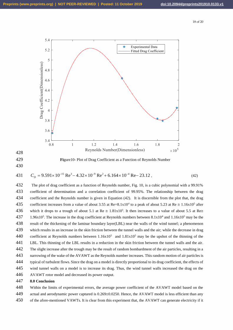
Figure10- Plot of Drag Coefficient as a Function of Reynolds Number 429

430

15 3 9 2 49.591 10 Re 4.32 10 Re 6.164 10 Re 23.12DC , (42) 431

The plot of drag coefficient as a function of Reynolds number, Fig. 10, is a cubic polynomial with a 99.91% 432

coefficient of determination and a correlation coefficient of 99.95%. The relationship between the drag 433

coefficient and the Reynolds number is given in Equation (42). It is discernible from the plot that, the drag 434

coefficient increases from a value of about 3.55 at Re=8.1x104 to a peak of about 5.23 at Re 1.16x105 after 435

which it drops to a trough of about 5.1 at Re 1.81x105. It then increases to a value of about 5.5 at Re 436

1.96x105. The increase in the drag coefficient at Reynolds numbers between 8.1x104 and 1.16x105 may be the 437

result of the thickening of the laminar boundary layer(LBL) near the walls of the wind tunnel; a phenomenon 438

which results in an increase in the skin friction between the tunnel walls and the air; while the decrease in drag 439

coefficient at Reynolds numbers between 1.16x105 and 1.81x105 may be the upshot of the thinning of the 440

LBL. This thinning of the LBL results in a reduction in the skin friction between the tunnel walls and the air. 441

The slight increase after the trough may be the result of random bombardment of the air particles, resulting in a 442

narrowing of the wake of the AVAWT as the Reynolds number increases. This random motion of air particles is 443

typical of turbulent flows. Since the drag on a model is directly proportional to its drag coefficient, the effects of 444

wind tunnel walls on a model is to increase its drag. Thus, the wind tunnel walls increased the drag on the 445

AVAWT rotor model and decreased its power output. 446

8.0 Conclusion 447

Within the limits of experimental errors, the average power coefficient of the AVAWT model based on the 448

actual and aerodynamic power captured is 0.2690.0250. Hence, the AVAWT model is less efficient than any 449

of the afore-mentioned VAWTs. It is clear from this experiment that, the AVAWT can generate electricity if it 450



19 of 20

is coupled with a generator. While it is difficult to make a good comparison between the AVAWT model used in 451

this experiment to existing VAWTs because, of the fact that, the AVAWT model is many times smaller than 452

existing VAWTs-something which rendered it incapable of generating enough torque; a better power 453

coefficient can be achieved using a larger size AVAWT and an open jet technique instead of testing in a wind 454

tunnel. The walls of the wind tunnel test section also increased the drag on the AVAWT, which subsequently 455

reduced its power output. A reduction in the drag on the AVAWT, could be achieved by using suitable airfoil 456

blades with rectangular slots at the trailing edges instead of the rolled sheet metal blades currently used. The slot 457

at the trailing edge of each airfoil blade will facilitate the flow of air through the blade from the positive pressure 458

side to the low-pressure side, thus, reducing the drag and increasing the lift on the blade. This phenomenon 459

which enhances flow from the high-pressure side to the low-pressure side through a slot at the trailing edge of 460

an airfoil is known as boundary layer suction. 461

Much work remains to be done in studying the performance characteristics of the AVAWT. This includes 462

numerical simulations and the quantification of the drag on the AVAWT using the wake speed distribution at 463

selected free stream speeds. 464

Funding: This research received no external funding. 465

Acknowledgments: The permission to use his prototype rotor in the experiment, the construction of supports for 466

instruments, the construction of the wind tunnel and the participation in the setup of the experiment by Bruce E. Anderson of 467

No Fossil Fuel LLC; 348 Baldwin Road, Odenton, Maryland is highly appreciated. 468

469

Conflicts of Interest: The authors declare no conflict of interest. 470

References 471

1. Zayas, J; 2011,” Scope of Wind Energy Generation Technologies”, Energy and Power Generation 472

Handbook by Rao K., R., ASME Press, Chap. 7. ISBN; 978-0-7918-5955-1 473

2. Manwell, J., F; McGowan, J, G; Rogers, A, L; 2011,” Wind Energy Explained (Theory, Design and 474

Applications)”, 2e, Wiley, Chaps. 1-3. ISBN:978-0-470-01500-1 475

3. Taylor, D; 2012,” Wind Energy”; Renewable Energy (Power for a Sustainable Future) 3e, by Boyle 476

G., Oxford Press, Chap.7. ISBN:978-0-19-954533-9 477

4. D’Ambrosio, M; Medaglia, M; 2010,” Vertical Axis Wind Turbines: History, Technology and 478

Applications”, Master’s Degree Thesis in Energy Engineering; Hogskolan Halmstadt 479

5. Wekesa, D; Wang, C; Wei, Y; Kamao, J; Damao, L; 2014” A Numerical Analysis of Unsteady Inflow 480

Wind for Site Specific Vertical Axis Wind Turbine: A Case Study for Marsabit and Garissa in Kenya”, 481

Renewable Energy, vol 76, Elsevier Ltd, pp 648-662. 482

6. Wekesa, D; Wang, C; Wei, Y; Damao, L; 2014,” Influence of Operating Conditions on Unsteady 483

Wind performance of Vertical Axis Wind Turbines Operating within a Fluctuating Free Stream: A 484

Numerical Study”, Journ. Engng. Ind. Aerodyn; vol135, Elsevier Ltd, pp76-89 485

7. Scheirich, F; Fletcher, T, M; Brown, R, E; 2010” Simulating the Aerodynamic Performance and Wake 486

Dynamics of a Vertical Axis Wind Turbine,” vol.14, Wind Energ., John Wiley, pp159-177, 487

8. Khan, J; Rhaman, M; 2014” Stress Analysis of Various Shaped Blade of Savonius Wind Turbine,” 488

ASME Paper No. IMECE2014-36307 489

9. Xisto C, M.; Pascoa J, C; Leger J, A; Transconi, M; 2014” Wind Energy Production Using an 490

Optimized Variable Pitch Vertical Axis Rotor. ASME Paper No. IMECE2014-38966 491

10. Mucke, T; Kleinhans, D; Peinke, J; 2010, “Atmospheric Turbulence and its Influence on the 492

Alternating Loads on Wind Turbines,” vol. 14, Wind Energ, Wiley, pp301-316 493



20 of 20

11. McPhee, D; Beyene, A; 2016, “The Straight-Bladed Morphing Vertical Axis Wind Turbine,” ASME 494

Paper No. Power2016-59192 495

12. McLaren, K; Tullis, S; Ziada, S; 2011,” Computational Fluid Dynamics of the Aerodynamics of a 496

High Solidity, Small Scale Vertical Axis Wind Turbine,” vol. 15, Wind Energ, Wiley, pp349-361 497

13. Scheurich, F; Brown, R., E; 2012,” Modelling the Aerodynamics of Vertical Axis Wind Turbines in 498

Unsteady Wind Conditions”, vol.16, Wind Energ., Wiley, pp91-107 499

14. Zanon, A; Giannattasio , P; Ferreirra, C., J., S; 2012, ” A Votex Panel Model for the Simulation of the 500

Wake Flow Past a Vertical Axis Wind Turbine in Dynamic Stall”, vol.16, Wind Energ2013, Wiley, 501

pp661-680 502

15. Jaohindy, P; Ennamiri, H; Garde, F; Bastide, A; 2013, “Numerical Investigation of Airflow Through a 503

Savonius Rotor,’ Vol 17, Wind Energ.2014, Wiley, PP853-869 504

16. Edwards, J; M., Danao, L; A., Howell, R., J; 2013, “PIV Measurements and CFD Simulation of the 505

performance and Flow Physics and a Small-Scale Vertical Axis Wind Turbine”’ vol 18, WIND 506

Energ2015, Wiley, pp201-217 507

17. Ragni, D; Ferreira, C., S; Correali, G., 2014,” Experimental Investigation of an Optimized Airfoil for 508

Vertical Axis Wind Turbines,” vol.18, Wind Energ., Wiley, pp1629-1643, 509

18. Kundu, P; K; Cohen, I., M; 2004, “Fluid Mechanics”, 3e, Elsevier Academic Press, Chap.4. 510

ISBN:978-0-12-178253-5 511

19. Aris, R.; 1989, “Vectors, Tensors and the Basic Equations of Fluid Mechanics” Dover edition, Chaps. 512

4 through 6. ISBN: 0-486-66110-5. 513

20. Graebel, W; P., 2007, “Advanced Fluid Mechanics”, Elsevier Academic Press, Chaps. 1 to 3. 514

ISBN:978-0-12-370885-4. 515

21. Damljanovia, D; Vukovic, D; Ocokoljic, G; Rasuo, B; 2016, “A Study of Wall interference effects in 516

Wind Tunnel Testing of a Standard Model at Transonic speeds”, Proc. ICAS 2016. 517

22. Mokhtar, W; Hasan, M., R; 2016, “A CFD Study of Wind Tunnel Wall Interference”, Proc. ASEE, N. 518

Central Section Conference. 519

23. Awbi, H, B; Tan, S, H; 1983, “Effects of Wind-Tunnel Walls on the Drag of a Sphere”, ASME Journ. 520

Of Fluids Engineering,103, pp. 461-465. DOI: 10.1115/ 1.3240816. 521

522



article experimental study of the performance of a novel

Documents