aroadmapforthecomputation ofpersistenthomology - …mason/papers/roadmap-fin… · ·...

Otter et al. EPJ Data Science (2017) 6:17 DOI 10.1140/epjds/s13688-017-0109-5

R E G U L A R A R T I C L E Open Access

A roadmap for the computationof persistent homologyNina Otter1,3, Mason A Porter4,1,2*, Ulrike Tillmann1,3, Peter Grindrod1 and Heather A Harrington1

*Correspondence:[email protected] of Mathematics,UCLA, Los Angeles, CA 90095, USAFull list of author information isavailable at the end of the article

AbstractPersistent homology (PH) is a method used in topological data analysis (TDA) to studyqualitative features of data that persist across multiple scales. It is robust toperturbations of input data, independent of dimensions and coordinates, andprovides a compact representation of the qualitative features of the input. Thecomputation of PH is an open area with numerous important and fascinatingchallenges. The field of PH computation is evolving rapidly, and new algorithms andsoftware implementations are being updated and released at a rapid pace. Thepurposes of our article are to (1) introduce theory and computational methods for PHto a broad range of computational scientists and (2) provide benchmarks ofstate-of-the-art implementations for the computation of PH. We give a friendlyintroduction to PH, navigate the pipeline for the computation of PH with an eyetowards applications, and use a range of synthetic and real-world data sets toevaluate currently available open-source implementations for the computation of PH.Based on our benchmarking, we indicate which algorithms and implementations arebest suited to different types of data sets. In an accompanying tutorial, we provideguidelines for the computation of PH. We make publicly available all scripts that wewrote for the tutorial, and we make available the processed version of the data setsused in the benchmarking.

Keywords: persistent homology; topological data analysis; point-cloud data;networks

1 IntroductionThe amount of available data has increased dramatically in recent years, and this situa-tion — which will only become more extreme — necessitates the development of inno-vative and efficient data-processing methods. Making sense of the vast amount of data isdifficult: on one hand, the sheer size of the data poses challenges; on the other hand, thecomplexity of the data, which includes situations in which data is noisy, high-dimensional,and/or incomplete, is perhaps an even more significant challenge. The use of clusteringtechniques and other ideas from areas such as computer science, machine learning, anduncertainty quantification — along with mathematical and statistical models — are oftenvery useful for data analysis (see, e.g., [–] and many other references). However, recentmathematical developments are shedding new light on such ‘traditional’ ideas, forging newapproaches of their own, and helping people to better decipher increasingly complicatedstructure in data.

© The Author(s) 2017. This article is distributed under the terms of the Creative Commons Attribution 4.0 International License(http://creativecommons.org/licenses/by/4.0/), which permits unrestricted use, distribution, and reproduction in any medium, pro-vided you give appropriate credit to the original author(s) and the source, provide a link to the Creative Commons license, andindicate if changes were made.

Otter et al. EPJ Data Science (2017) 6:17 of 38

Techniques from the relatively new subject of ‘topological data analysis’ (TDA) have pro-vided a wealth of new insights in the study of data in an increasingly diverse set of applica-tions — including sensor-network coverage [], proteins [–], -dimensional structureof DNA [], development of cells [], stability of fullerene molecules [], robotics [–], signals in images [, ], periodicity in time series [], cancer [–], phylogenetics[–], natural images [], the spread of contagions [, ], self-similarity in geometry[], materials science [–], financial networks [, ], diverse applications in neuro-science [–], classification of weighted networks [], collaboration networks [, ],analysis of mobile phone data [], collective behavior in biology [], time-series outputof dynamical systems [], natural-language analysis [], and more. There are numerousothers, and new applications of TDA appear in journals and preprint servers increasinglyfrequently. There are also interesting computational efforts, such as [].

TDA is a field that lies at the intersection of data analysis, algebraic topology, compu-tational geometry, computer science, statistics, and other related areas. The main goal ofTDA is to use ideas and results from geometry and topology to develop tools for studyingqualitative features of data. To achieve this goal, one needs precise definitions of qualita-tive features, tools to compute them in practice, and some guarantee about the robustnessof those features. One way to address all three points is a method in TDA called persistenthomology (PH). This method is appealing for applications because it is based on algebraictopology, which gives a well-understood theoretical framework to study qualitative fea-tures of data with complex structure, is computable via linear algebra, and is robust withrespect to small perturbations in input data.

Types of data sets that can be studied with PH include finite metric spaces, digital im-ages, level sets of real-valued functions, and networks (see Section .). In the next twoparagraphs, we give some motivation for the main ideas of persistent homology by dis-cussing two examples of such data sets.

Finite metric spaces are also called point-cloud data sets in the TDA literature. From atopological point of view, finite metric spaces do not contain any interesting information.One thus considers a thickening of a point cloud at different scales of resolution and thenanalyzes the evolution of the resulting shape across the different resolution scales. Thequalitative features are given by topological invariants, and one can represent the variationof such invariants across the different resolution scales in a compact way to summarize the‘shape’ of the data.

As an illustration, consider the set of points in R that we show in Figure . Let ϵ, whichwe interpret as a distance parameter, be a nonnegative real number (so ϵ = gives the setof points). For different values of ϵ, we construct a space Sϵ composed of vertices, edges,triangles, and higher-dimensional polytopes according to the following rule: We includean edge between two points i and j if and only if the Euclidean distance between them isno larger than ϵ; we include a triangle if and only if all of its edges are in Sϵ ; we includea tetrahedron if and only if all of its face triangles are in Sϵ ; and so on. For ϵ ≤ ϵ′, it thenfollows that the space Sϵ is contained in the space Sϵ′ . This yields a nested sequence ofspaces, as we illustrate in Figure (a). Our construction of nested spaces gives an exampleof a ‘filtered Vietoris–Rips complex,’ which we define and discuss in Section ..

By using homology, a tool in algebraic topology, one can measure several features of thespaces Sϵ — including the numbers of components, holes, and voids (higher-dimensionalversions of holes). One can then represent the lifetime of such features using a finite collec-


Figure 1 Example of persistent homology for a point cloud. (a) A finite set of points in R2 (for ϵ = 0) anda nested sequence of spaces obtained from it (from ϵ = 0 to ϵ = 2.1). (b) Barcode for the nested sequence ofspaces illustrated in (a). Solid lines represent the lifetime of components, and dashed lines represent thelifetime of holes.

tion of intervals known as a ‘barcode.’ Roughly, the left endpoint of an interval representsthe birth of a feature, and its right endpoint represents the death of the same feature. InFigure (b), we reproduce such intervals for the number of components (blue solid lines)and the number of holes (violet dashed lines). In Figure (b), we observe a dashed linethat is significantly longer than the other dashed lines. This indicates that the data set hasa long-lived hole. By contrast, in this example one can potentially construe the shorterdashed lines as noise. (However, note that while widespread, such an intepretation is notcorrect in general; for applications in which one considers some short and medium-sizedintervals as features rather than noise, see [, ].) When a feature is still ‘alive’ at thelargest value of ϵ that we consider, the lifetime interval is an infinite interval, which weindicate by putting an arrowhead at the right endpoint of the interval. In Figure (b), wesee that there is exactly one solid line that lives up to ϵ = .. One can use informationabout shorter solid lines to extract information about how data is clustered in a similarway as with linkage-clustering methods [].

One of the most challenging parts of using PH is statistical interpretation of results.From a statistical point of view, a barcode like the one in Figure (b) is an unknown quantitythat one is trying to estimate; one therefore needs methods for quantitatively assessing thequality of the barcodes that one obtains with computations. The challenge is twofold. Onone hand, there is a cultural obstacle: practitioners of TDA often have backgrounds inpure topology and are not well-versed in statistical approaches to data analysis []. Onthe other hand, the space of barcodes lacks geometric properties that would make it easyto define basic concepts such as mean, median, and so on. Current research is focusedboth on studying geometric properties of this space and on studying methods that mapthis space to spaces that have better geometric properties for statistics. In Section ., wegive a brief overview of the challenges and current approaches for statistical interpretationof barcodes. This is an active area of research and an important endeavor, as few statisticaltools are currently available for interpreting results in applications of PH.

We now discuss a second example related to digital images. (For an illustration, see Fig-ure (a).) Digital images have a cubical structure, given by the pixels (for -dimensional


Figure 2 Example of persistent homology for a gray-scale digital image. (a) A gray-scale image, (b) thematrix of gray values, (c) the filtered cubical complex associated to the digital image, and (d) the barcode forthe nested sequence of spaces in panel (c). A solid line represents the lifetime of a component, and a dashedline represents the lifetime of a hole.

digital images) or voxels (for -dimensional images). Therefore, one approach to studydigital images uses combinatorial structures called ‘cubical complexes.’ (For a different ap-proach to the study of digital images, see Section ..) Roughly, cubical complexes are topo-logical spaces built from a union of vertices, edges, squares, cubes, and higher-dimensionalhypercubes. An efficient way [] to build a cubical complex from a -dimensional digitalimage consists of assigning a vertex to every pixel, then joining vertices corresponding toadjacent pixels by an edge, and filling in the resulting squares. One proceeds in a similarway for -dimensional images. One then labels every vertex with an integer that corre-sponds to the gray value of the pixel, and one labels edges (respectively, squares) withthe maximum of the values of the adjacent vertices (respectively, edges). One can thenconstruct a nested sequence of cubical complexes C ⊂ C ⊂ · · · ⊂ C, where for eachi ∈ {, , . . . , }, the cubical complex Ci contains all vertices, edges, squares, and cubesthat are labeled by a number less than or equal to i. (See Figure (c) for an example.) Sucha sequence of cubical complexes is also called a ‘filtered cubical complex.’ Similar to theprevious example, one can use homology to measure several features of the spaces Ci (seeFigure (d)).

In the present article, we focus on persistent homology, but there are also other methodsin TDA — including the Mapper algorithm [], Euler calculus (see [] for an introduc-tion with an eye towards applications), cellular sheaves [, ], and many more. We referreaders who wish to learn more about the foundations of TDA to the article [], whichdiscusses why topology and functoriality are essential for data analysis. We point to severalintroductory papers, books, and two videos on PH at the end of Section .

The first algorithm for the computation of PH was introduced for computation overF (the field with two elements) in [] and over general fields in []. Since then, sev-eral algorithms and optimization techniques have been presented, and there are now var-ious powerful implementations of PH [–]. Those wishing to try PH for computations


may find it difficult to discern which implementations and algorithms are best suited fora given task. The field of PH is evolving continually, and new software implementationsand updates are released at a rapid pace. Not all of them are well-documented, and (as iswell-known in the TDA community), the computation of PH for large data sets is compu-tationally very expensive.

To our knowledge, there exists neither an overview of the various computational meth-ods for PH nor a comprehensive benchmarking of the state-of-the-art implementationsfor the computation of persistent homology. In the present article, we close this gap: weintroduce computation of PH to a general audience of applied mathematicians and compu-tational scientists, offer guidelines for the computation of PH, and test the existing open-source published libraries for the computation of PH.

The rest of our paper is organized as follows. In Section , we discuss related work. Wethen introduce homology in Section and introduce PH in Section . We discuss the var-ious steps of the pipeline for the computation of PH in Section , and we briefly examinealgorithms for generalized persistence in Section . In Section , we give an overview ofsoftware libraries, discuss our benchmarking of a collection of them, and provide guide-lines for which software or algorithm is better suited to which data set. (We provide spe-cific guidelines for the computation of PH with the different libraries in the Tutorial inAdditional file of the Supplementary Information (SI).) In Section , we discuss futuredirections for the computation of PH.

2 Related workIn our work, we introduce PH to non-experts with an eye towards applications, and webenchmark state-of-the-art libraries for the computation of PH. In this section, we discussrelated work for both of these points.

There are several excellent introductions to the theory of PH (see the references at theend of Section .), but none of them emphasizes the actual computation of PH by pro-viding specific guidelines for people who want to do computations. In the present paper,we navigate the theory of PH with an eye towards applications, and we provide guidelinesfor the computation of PH using the open-source libraries JAVAPLEX, PERSEUS, DIONY-SUS, DIPHA, GUDHI, and RIPSER. We include a tutorial (see Additional file of the SI) thatgives specific instructions for how to use the different functionalities that are implementedin these libraries. Much of this information is scattered throughout numerous different pa-pers, websites, and even source code of implementations, and we believe that it is benefi-cial to the applied mathematics community (especially people who seek an entry point intoPH) to find all of this information in one place. The functionalities that we cover includeplots of barcodes and persistence diagrams and the computation of PH with Vietoris–Ripscomplexes, alpha complexes, Čech complexes, witness complexes, cubical complexes forimage data. We also discuss the computation of the bottleneck and Wasserstein distances.We thus believe that our paper closes a gap in introducing PH to people interested inapplications, while our tutorial complements existing tutorials (see, e.g. [–]).

We believe that there is a need for a thorough benchmarking of the state-of-the-art li-braries. In our work, we use twelve different data sets to test and compare the librariesJAVAPLEX, PERSEUS, DIONYSUS, DIPHA, GUDHI, and RIPSER. There are several bench-markings in the PH literature; we are aware of the following ones: the benchmarking in[] compares the implementations of standard and dual algorithms in DIONYSUS; the one


in [] compares the Morse-theoretic reduction algorithm with the standard algorithm;the one in [] compares all of the data structures and algorithms implemented in PHAT;the benchmarking in [] compares PHAT and its spin-off DIPHA; and the benchmarkingin C. Maria’s doctoral thesis [] is to our knowledge the only existing benchmarking thatcompares packages from different authors. However, Maria compares only up to three dif-ferent implementations at one time, and he used the package JPLEX (which is no longermaintained) instead of the JAVAPLEX library (its successor). Additionally, the widely usedlibrary PERSEUS (e.g., it was used in [, , , ]) does not appear in Maria’s bench-marking.

3 HomologyAssume that one is given data that lies in a metric space, such as a subset of Euclideanspace with an inherited distance function. In many situations, one is not interested in theprecise geometry of these spaces, but instead seeks to understand some basic character-istics, such as the number of components or the existence of holes and voids. Algebraictopology captures these basic characteristics either by counting them or by associatingvector spaces or more sophisticated algebraic structures to them. Here we are interestedin homology, which associates one vector space Hi(X) to a space X for each natural num-ber i ∈ {, , , . . . }. The dimension of H(X) counts the number of path components in X,the dimension of H(X) is a count of the number of holes, and the dimension of H(X) is acount of the number of voids. An important property of these algebraic structures is thatthey are robust, as they do not change when the underlying space is transformed by bend-ing, stretching, or other deformations. In technical terms, they are homotopy invariant.a

It can be very difficult to compute the homology of arbitrary topological spaces. Wethus approximate our spaces by combinatorial structures called ‘simplicial complexes,’ forwhich homology can be easily computed algorithmically. Indeed, often one is not evengiven the space X, but instead possesses only a discrete sample set S from which to builda simplicial complex following one of the recipes described in Sections . and ..

3.1 Simplicial complexes and their homologyWe begin by giving the definitions of simplicial complexes and of the maps between them.Roughly, a simplicial complex is a space that is built from a union of points, edges, tri-angles, tetrahedra, and higher-dimensional polytopes. We illustrate the main definitionsgiven in this section with the example in Figure . As we pointed out in Section , ‘cubicalcomplexes’ give another way to associate a combinatorial structure to a topological space.In TDA, cubical complexes have been used primarily to study image data sets. One cancompute PH for a nested sequence of cubical complexes in a similar way as for simplicialcomplexes, but the theory of PH for simplicial complexes is richer, and we therefore exam-ine only simplicial homology and complexes in our discussions. See [] for a treatmentof cubical complexes and their homology.

Definition A simplicial complexb is a collection K of non-empty subsets of a set K suchthat {v} ∈ K for all v ∈ K, and τ ⊂ σ and σ ∈ K guarantees that τ ∈ K . The elements ofK are called vertices of K , and the elements of K are called simplices. Additionally, we saythat a simplex has dimension p or is a p-simplex if it has a cardinality of p + . We use Kpto denote the collection of p-simplices. The k-skeleton of K is the union of the sets Kp for


Figure 3 A simple example. (a) A simplicial complex, (b) a map of simplicial complexes, and (c) a geometricrealization of the simplicial complex in (a).

all p ∈ {, , . . . , k}. If τ and σ are simplices such that τ ⊂ σ , then we call τ a face of σ , andwe say that τ is a face of σ of codimension k′ if the dimensions of τ and σ differ by k′. Thedimension of K is defined as the maximum of the dimensions of its simplices. A map ofsimplicial complexes, f : K → L, is a map f : K → L such that f (σ ) ∈ L for all σ ∈ K .

We give an example of a simplicial complex in Figure (a) and an example of a map ofsimplicial complexes in Figure (b). Definition is rather abstract, but one can alwaysinterpret a finite simplicial complex K geometrically as a subset of RN for sufficientlylarge N ; such a subset is called a ‘geometric realization,’ and it is unique up to a canon-ical piecewise-linear homeomorphism. For example, the simplicial complex in Figure (a)has a geometric realization given by the subset of R in Figure (c).

We now define homology for simplicial complexes. Let F denote the field with twoelements. Given a simplicial complex K , let Cp(K) denote the F-vector space with basisgiven by the p-simplices of K . For any p ∈ {, , . . . }, we define the linear map (on the basiselements)

dp : Cp(K) → Cp–(K),

σ &→!

τ⊂σ ,τ∈Kp–

τ .

For p = , we define d to be the zero map. In words, dp maps each p-simplex to its bound-ary, the sum of its faces of codimension . Because the boundary of a boundary is alwaysempty, the linear maps dp have the property that composing any two consecutive mapsyields the zero map: for all p ∈ {, , , . . . }, we have dp ◦ dp+ = . Consequently, the im-age of dp+ is contained in the kernel of dp, so we can take the quotient of kernel(dp) byimage(dp+). We can thus make the following definition.

Definition For any p ∈ {, , , . . . }, the pth homology of a simplicial complex K is thequotient vector space

Hp(K) := kernel(dp)/ image(dp+).


Figure 4 Examples to illustrate simplicial homology. (a) Computation of simplicial homology for thesimplicial complex in Figure 3(a) and (b) induced map in 0th homology for the map of simplicial complexes inFigure 3(b).

Its dimension

βp(K) := dim Hp(K) = dim kernel(dp) – dim image(dp+)

is called the pth Betti number of K . Elements in the image of dp+ are called p-boundaries,and elements in the kernel of dp are called p-cycles.

Intuitively, the p-cycles that are not boundaries represent p-dimensional holes. There-fore, the pth Betti number ‘counts’ the number of p-holes. Additionally, if K is a simplicialcomplex of dimension n, then for all p > n, we have that Hp(K) = , as Kp is empty andhence Cp(K) = . We therefore obtain the following sequence of vector spaces and linearmaps:

dn+−→ Cn(K)

dn−→ · · ·d−→ C(K)

d−→ C(K)d−→ .

We give an example of such a sequence in Figure (a), for which we also report the Bettinumbers.

One of the most important properties of simplicial homology is ‘functoriality.’ Any mapf : K → K ′ of simplicial complexes induces the following F-linear map:

"fp : Cp(K) → Cp#K ′$,

!

σ∈Kp

cσ σ &→!

σ∈Kp such that f (σ )∈K ′p

cσ f (σ ) for any p ∈ {, , , . . . },


where cσ ∈ F. Additionally, "fp ◦ dp+ = d′p+ ◦"fp+, and the map "fp therefore induces the

following linear map between homology vector spaces:

fp : Hp(K) → Hp#K ′$,

[c] &→%"fp(c)

&.

(We give an example of such a map in Figure (b).) Consequently, to any map f : K → K ′

of simplicial complexes, we can assign a map fp : Hp(K) → Hp(K ′) for any p ∈ {, , , . . . }.This assignment has the important property that given a pair of composable maps of sim-plicial complexes, f : K → K ′ and g : K ′ → K ′′, the map (g ◦ f )p : Hp(K) → Hp(K ′′) is equalto the composition of the maps induced by f and g . That is, (g ◦ f )p = gp ◦ fp. The fact thata map of simplicial complexes induces a map on homology that is compatible with com-position is called functoriality, and it is crucial for the definition of persistent homology(see Section .).

When working with simplicial complexes, one can modify a simplicial complex by re-moving or adding a pair of simplices (σ , τ ), where τ is a face of σ of codimension and σ isthe only simplex that has τ as a face. The resulting simplicial complex has the same homol-ogy as the one with which we started. In Figure (a), we can remove the pair ({a, b, c}, {b, c})and then the pair ({a, b}, {b}) without changing the Betti numbers. Such a move is calledan elementary simplicial collapse []. In Section .., we will see an application of thisfor the computation of PH.

In this section, we have defined simplicial homology over the field F — i.e., ‘with co-efficients in F.’ One can be more general and instead define simplicial homology withcoefficients in any field (or even in the integers). However, when = –, one needs to takemore care when defining the boundary maps dp to ensure that dp ◦ dp+ remains the zeromap. Consequently, the definition is more involved. For the purposes of the present pa-per, it suffices to consider homology with coefficients in the field F. Indeed, we will seein Section that to obtain topological summaries in the form of barcodes, we need tocompute homology with coefficients in a field. Furthermore, as we summarize in Table (in Section ), most of the implementations for the computation of PH work with F.

We conclude this section with a warning: changing the coefficient field can affect theBetti numbers. For example, if one computes the homology of the Klein bottle (see Sec-tion ..) with coefficients in the field Fp with p elements, where p is a prime, thenβ(K) = for all primes p. However, β(K) = and β(K) = if p = , but β(K) = andβ(K) = for all other primes p. The fact that β(K) = for p = arises from the nonori-entability of the Klein bottle. The treatment of different coefficient fields is beyond thescope of our article, but interested readers can peruse [] for an introduction to homol-ogy and [] for an overview of computational homology.

3.2 Building simplicial complexesAs we discussed in Section ., computing the homology of finite simplicial complexesboils down to linear algebra. The same is not true for the homology of an arbitrary spaceX, and one therefore tries to find simplicial complexes whose homology approximates thehomology of the space in an appropriate sense.

An important tool is the Čech (Č) complex. Let U be a cover of X — i.e., a collection ofsubsets of X such that the union of the subsets is X. The k-simplices of the Čech complex


are the non-empty intersections of k + sets in the cover U . More precisely, we define thenerve of a collection of sets as follows.

Definition Let U = {Ui}i∈I be a non-empty collection of sets. The nerve of U is thesimplicial complex with set of vertices given by I and k-simplices given by {i, . . . , ik} ifand only if Ui ∩ · · · ∩ Uik = ∅.

If the cover of the sets is sufficiently ‘nice,’ then the Nerve Theorem implies that the nerveof the cover and the space X have the same homology [, ]. For example, suppose thatwe have a finite set of points S in a metric space X. We then can define, for every ϵ > ,the space Sϵ as the union '

x∈S B(x, ϵ), where B(x, ϵ) denotes the closed ball with radius ϵ

centered at x. It follows that {B(x, ϵ) | x ∈ S} is a cover of Sϵ , and the nerve of this coveris the Čech complex on S at scale ϵ. We denote this complex by Cϵ(S). If the space X isEuclidean space, then the Nerve Theorem guarantees that the simplicial complex Cϵ(S)recovers the homology of Sϵ .

From a computational point of view, the Čech complex is expensive because one has tocheck for large numbers of intersections. Additionally, in the worst case, the Čech complexcan have dimension |U |– , and it therefore can have many simplices in dimensions higherthan the dimension of the underlying space. Ideally, it is desirable to construct simplicialcomplexes that approximate the homology of a space but are easy to compute and have‘few’ simplices, especially in high dimensions. This is a subject of ongoing research: In Sec-tion ., we give an overview of state-of-the-art methods to associate complexes to point-cloud data in a way that addresses one or both of these desiderata. See [, ] for more de-tails on the Čech complex, and see [, ] for a precise statement of the Nerve Theorem.

4 Persistent homologyAssume that we are given experimental data in the form of a finite metric space S; thereare points or vectors that represent measurements along with some distance function(e.g., given by a correlation or a measure of dissimilarity) on the set of points or vectors.Whether or not the set S is a sample from some underlying topological space, it is usefulto think of it in those terms. Our goal is to recover the properties of such an underlyingspace in a way that is robust to small perturbations in the data S. In a broad sense, this isthe subject of topological inference. (See [] for an overview.) If S is a subset of Euclideanspace, one can consider a ‘thickening’ Sϵ of S given by the union of balls of a certain fixedradius ϵ around its points and then compute the Čech complex. One can thus try to com-pute qualitative features of the data set S by constructing the Čech complex for a chosenvalue ϵ and then computing its simplicial homology. The problem with this approach isthat there is a priori no clear choice for the value of the parameter ϵ. The key insight ofPH is the following: To extract qualitative information from data, one considers several (oreven all) possible values of the parameter ϵ. As the value of ϵ increases, simplices are addedto the complexes. Persistent homology then captures how the homology of the complexeschanges as the parameter value increases, and it detects which features ‘persist’ acrosschanges in the parameter value. We give an example of persistent homology in Figure .

4.1 Filtered complexes and homologyLet K be a finite simplicial complex, and let K ⊂ K ⊂ · · · ⊂ Kl = K be a finite sequenceof nested subcomplexes of K . The simplicial complex K with such a sequence of sub-


Figure 5 Example of persistent homology for a finite filtered simplicial complex. (a) We start with afinite filtered simplicial complex. (b) At each filtration step i, we draw as many vertices as the dimension of(left column) H0(Ki) and (right column) H1(Ki). We label the vertices by basis elements, the existence of whichis guaranteed by the Fundamental Theorem of Persistent Homology, and we draw an edge between twovertices to represent the maps fi,j , as explained in the main text. We thus obtain a well-defined collection ofdisjoint half-open intervals called a ‘barcode.’ We interpret each interval in degree p as representing thelifetime of a p-homology class across the filtration. (c) We rewrite the diagram in (b) in the conventional way.We represent classes that are born but do not die at the final filtration step using arrows that start at the birthof that feature and point to the right. (d) An alternative graphical way to represent barcodes (which givesexactly the same information) is to use persistence diagrams, in which an interval [i, j) is represented by thepoint (i, j) in the extended plane R2

, where R = R ∪ {∞}. Therefore, a persistence diagram is a finite multisetof points in R2

. We use squares to signify the classes that do not die at the final step of a filtration, and the sizeof dots or squares is directly proportional to the number of points being represented. For technical reasons,which we discuss briefly in Section 5.4, one also adds points on the diagonal to the persistence diagrams.(Each of the points on the diagonal has infinite multiplicity.)

complexes is called a filtered simplicial complex. See Figure (a) for an example of filteredsimplicial complex. We can apply homology to each of the subcomplexes. For all p, theinclusion maps Ki → Kj induce F-linear maps fi,j : Hp(Ki) → Hp(Kj) for all i, j ∈ {, . . . , l}with i ≤ j. By functoriality (see Section .), it follows that

fk,j ◦ fi,k = fi,j for all i ≤ k ≤ j. ()

We therefore give the following definition.c


Definition Let K ⊂ K ⊂ · · · ⊂ Kl = K be a filtered simplicial complex. The pth persis-tent homology of K is the pair

#(Hp(Ki)

)≤i≤l, {fi,j}≤i≤j≤l

$,

where for all i, j ∈ {, . . . , l} with i ≤ j, the linear maps fi,j : Hp(Ki) → Hp(Kj) are the mapsinduced by the inclusion maps Ki → Kj.

The pth persistent homology of a filtered simplicial complex gives more refined informa-tion than just the homology of the single subcomplexes. We can visualize the informationgiven by the vector spaces Hp(Ki) together with the linear maps fi,j by drawing the followingdiagram: at filtration step i, we draw as many bullets as the dimension of the vector spaceHp(Ki). We then connect the bullets as follows: we draw an interval between bullet u at fil-tration step i and bullet v at filtration step i + if the generator of Hp(Ki) that correspondsto u is sent to the generator of Hp(Ki+) that corresponds to v. If the generator correspond-ing to a bullet u at filtration step i is sent to by fi,i+, we draw an interval starting at uand ending at i + . (See Figure (b) for an example.) Such a diagram clearly depends ona choice of basis for the vector spaces Hp(Ki), and a poor choice can lead to complicatedand unreadable clutter. Fortunately, by the Fundamental Theorem of Persistent Homology[], there is a choice of basis vectors of Hp(Ki) for each i ∈ {, . . . , l} such that one can con-struct the diagram as a well-defined and unique collection of disjoint half-open intervals,collectively called a barcode.d We give an example of a barcode in Figure (c). Note thatthe Fundamental Theorem of PH, and hence the existence of a barcode, relies on the factthat we are using homology with field coefficients. (See [] for more details.)

There is a useful interpretation of barcodes in terms of births and deaths of generators.Considering the maps fi,j written in the basis given by the Fundamental Theorem of Per-sistent Homology, we say that x ∈ Hp(Ki) (with x = ) is born in Hp(Ki) if it is not in theimage of fi–,i (i.e., f –

i–,i(x) = ∅). For x ∈ Hp(Ki) (with x = ), we say that x dies in Hp(Kj) ifj > i is the smallest index for which fi,j(x) = . The lifetime of x is represented by the half-open interval [i, j). If fi,j(x) = for all j such that i < j ≤ l, we say that x lives forever, and itslifetime is represented by the interval [i,∞).

Remark Note that some references (e.g., []) introduce persistent homology by defin-ing the birth and death of generators without using the existence of a choice of compatiblebases, as given by the Fundamental Theorem of Persistent Homology. The definition ofbirth coincides with the definition that we have given, but the definition of death is dif-ferent. One says that x ∈ Hp(Ki) (with x = ) dies in Hp(Kj) if j > i is the smallest indexfor which either fi,j(x) = or there exists y ∈ Hp(Ki′ ) with i′ < i such that fi′ ,j(y) = fi,j(x). Inwords, this means that x and y merge at filtration step j, and the class that was born earlieris the one that survives. In the literature, this is called the elder rule. We do not adopt thisdefinition, because the elder rule is not well-defined when two classes are born at the sametime, as there is no way to choose which class will survive. For example, in Figure , thereare two classes in H that are born at the same stage in K. These two classes merge in K,but neither dies. The class that dies is [a] + [c].

There are numerous excellent introductions to PH, such as the books [, , , ]and the papers [, –]. For a brief and friendly introduction to PH and some of


Figure 6 PH pipeline.

its applications, see the video https://www.youtube.com/watch?v=hbnGWavag. For abrief introduction to some of the ideas in TDA, see the video https://www.youtube.com/watch?v=XfWibrhstw.

5 Computation of PH for dataWe summarize the pipeline for the computation of PH from data in Figure . In the fol-lowing subsections, we describe each step of this pipeline and state-of-the-art algorithmsfor the computation of PH. The two features that make PH appealing for applications arethat it is computable via linear algebra and that it is stable with respect to perturbationsin the measurement of data. In Section ., we give a brief overview of stability results.

5.1 DataAs we mentioned in Section , types of data sets that one can study with PH include finitemetric spaces, digital images, and networks. We now give a brief overview of how one canstudy these types of data sets using PH.

.. NetworksOne can construe an undirected network as a -dimensional simplicial complex. If thenetwork is weighted, then filtering by increasing or decreasing weight yields a filtered -dimensional simplicial complex. To obtain more refined information about the network,it is desirable to construct higher-dimensional simplices. There are various methods to dothis. The simplest method, called a weight rank clique filtration (WRCF), consists of build-ing a clique complex on each subnetwork. (See Section .. for the definition of ‘cliquecomplex.’) See [] for an application of this method. Another method to study networkswith PH consists of mapping the nodes of the network to points of a finite metric space.There are several ways to compute distances between nodes of a network; the methodthat we use in our benchmarking in Section consists of computing a shortest path be-tween nodes. For such a distance to be well-defined, note that one needs the network tobe connected (although conventionally one takes the distance between nodes in differentcomponents to be infinity). There are many methods to associate an unfiltered simplicialcomplex to both undirected and directed networks. See the book [] for an overview ofsuch methods, and see the paper [] for an overview of PH for networks.

.. Digital imagesAs we mentioned in Section , digital images have a natural cubical structure: -dimensional digital images are made of pixels, and -dimensional images are made ofvoxels. Therefore, to study digital images, cubical complexes are more appropriate thansimplicial complexes. Roughly, cubical complexes are spaces built from a union of vertices,edges, squares, cubes, and so on. One can compute PH for cubical complexes in a similarway as for simplicial complexes, and we will therefore not discuss this further in this paper.See [] for a treatment of computational homology with cubical complexes rather thansimplicial complexes and for a discussion of the relationship between simplicial and cubi-cal homology. See [] for an efficient algorithm and data structure for the computation


of PH for cubical data, and [] for an algorithm that computes PH for cubical data in anapproximate way. For an application of PH and cubical complexes to movies, see [].

Other approaches for studying digital images are also useful. In general, given a digitalimage that consists of N pixels or voxels, one can consider this image as a point in a c×N-dimensional space, with each coordinate storing a vector of length c representing the colorof a pixel or voxel. Defining an appropriate distance function on such a space allows oneto consider a collection of images (each of which has N pixels or voxels) as a finite metricspace. A version of this approach was used in [], in which the local structure of naturalimages was studied by selecting × patches of pixels of the images.

.. Finite metric spacesAs we mentioned in the previous two subsections, both undirected networks and imagedata can be construed as finite metric spaces. Therefore, methods to study finite metricspaces with PH apply to the study of networks and image data sets.

In some applications, points of a metric space have associated ‘weights.’ For instance, inthe study of molecules, one can represent a molecule as a union of balls in Euclidean space[, ]. For such data sets, one would therefore also consider a minimum filtration value(see Section . for the description of such filtration values) at which the point enters thefiltration. In Table (g), we indicate which software libraries implement this feature.

5.2 Filtered simplicial complexesIn Section ., we introduced the Čech complex, a classical simplicial complex from alge-braic topology. However, there are many other simplicial complexes that are better suitedfor studying data from applications. We discuss them in this section.

To be a useful tool for the study of data, a simplicial complex has to satisfy some theoreti-cal properties dictated by topological inference; roughly, if we build the simplicial complexon a set of points sampled from a space, then the homology of the simplicial complex hasto approximate the homology of the space. For the Čech complex, these properties areguaranteed by the Nerve Theorem. Some of the complexes that we discuss in this sub-section are motivated by a ‘sparsification paradigm’: they approximate the PH of knownsimplicial complexes but have fewer simplices than them. Others, like the Vietoris–Ripscomplex, are appealing because they can be computed efficiently. In this subsection, wealso review reduction techniques, which are heuristics that reduce the size of complexeswithout changing the PH. In Table , we summarize the simplicial complexes that we dis-cuss in this subsection.

Table 1 We summarize several types of complexes that are used for PH

Complex K Size of K Theoretical guarantee

Cech 2O(N) Nerve theoremVietoris–Rips (VR) 2O(N) Approximates Cech complexAlpha NO(⌈d/2⌉) (N points in Rd) Nerve theoremWitness 2O(|L|) For curves and surfaces in Euclidean spaceGraph-induced complex 2O(|Q|) Approximates VR complexSparsified Cech O(N) Approximates Cech complexSparsified VR O(N) Approximates VR complex

We indicate the theoretical guarantees and the worst-case sizes of the complexes as functions of the cardinality N of thevertex set. For the witness complexes (see Section 5.2.4), L denotes the set of landmark points, while Q denotes thesubsample set for the graph-induced complex (see Section 5.2.5).


For the rest of this subsection (X, d) denotes a metric space, and S is a subset of X, whichbecomes a metric space with the induced metric. In applications, S is the collection of mea-surements together with a notion of distance, and we assume that S lies in the (unknown)metric space X. Our goal is then to compute persistent homology for a sequence of nestedspaces Sϵ , Sϵ , . . . , Sϵl , where each space gives a ‘thickening’ of S in X.

.. Vietoris–Rips complexWe have seen that one of the disadvantages of the Čech complex is that one has to checkfor a large number of intersections. To circumvent this issue, one can instead consider theVietoris–Rips (VR) complex, which approximates the Čech complex. For a non-negativereal number ϵ, the Vietoris–Rips complex VRϵ(S) at scale ϵ is defined as

VRϵ(S) =(σ ⊆ S | d(x, y) ≤ ϵ for all x, y ∈ σ

).

The sense in which the VR complex approximates the Čech complex is that, when S is asubset of Euclidean space, we have Cϵ(S) ⊆ VRϵ(S) ⊆ C√

ϵ(S). Deciding whether a subsetσ ⊆ S is in VRϵ(S) is equivalent to deciding if the maximal pairwise distance between anytwo vertices in σ is at most ϵ. Therefore, one can construct the VR complex in two steps.One first computes the ϵ-neighborhood graph of S. This is the graph whose vertices are allpoints in S and whose edges are

((i, j) ∈ S × S | i = j and d(i, j) ≤ ϵ

).

Second, one obtains the VR complex by computing the clique complex of the ϵ-neighborhood graph. The clique complex of a graph is a simplicial complex that is de-fined as follows: The subset {x, . . . , xk} is a k-simplex if and only if every pair of verticesin {x, . . . , xk} is connected by an edge. Such a collection of vertices is called a clique. Thisconstruction makes it very easy to compute the VR complex, because to construct theclique complex one has only to check for pairwise distances — for this reason, cliquecomplexes are also called ‘lazy’ in the literature. Unfortunately, the VR complex has thesame worst-case complexity as the Čech complex. In the worst case, it can have up to|S| – simplices and dimension |S| – .

In applications, one therefore usually only computes the VR complex up to some dimen-sion k ≪ |S| – . In our benchmarking, we often choose k = and k = .

The paper [] overviews different algorithms to perform both of the steps for the con-struction of the VR complex, and it introduces fast algorithms to construct the cliquecomplex. For more details on the VR complex, see [, ]. For a proof of the approxima-tion of the Čech complex by the VR complex, see []; see [] for a generalization of thisresult.

.. The Delaunay complexTo avoid the computational problems of the Čech and VR complexes, we need a way tolimit the number of simplices in high dimensions. The Delaunay complex gives a geo-metric tool to accomplish this task, and most of the new simplicial complexes that havebeen introduced for the study of data are based on variations of the Delaunay complex.The Delaunay complex and its dual, the Voronoi diagram, are central objects of study incomputational geometry because they have many useful properties.


For the Delaunay complex, one usually considers X = Rd , so we also make this assump-tion. We subdivide the space Rd into regions of points that are closest to any of the pointsin S. More precisely, for any s ∈ S, we define

Vs =(

x ∈ Rd | d(x, s) ≤ d#x, s′$ for all s′ ∈ S

).

The collection of sets Vs is a cover for Rd that is called the Voronoi decomposition of Rd

with respect to S, and the nerve of this cover is called the Delaunay complex of S andis denoted by Del(S; Rd). In general, the Delaunay complex does not have a geometricrealization in Rd . However, if the points S are ‘in general position’e then the Delaunaycomplex has a geometric realization in Rd that gives a triangulation of the convex hullof S. In this case, the Delaunay complex is also called the Delaunay triangulation.

The complexity of the Delaunay complex depends on the dimension d of the space. Ford ≤ , the best algorithms have complexity O(N log N), where N is the cardinality of S.For d ≥ , they have complexity O(N⌈d/⌉). The construction of the Delaunay complex istherefore costly in high dimensions, although there are efficient algorithms for the com-putation of the Delaunay complex for d = and d = . Developing efficient algorithms forthe construction of the Delaunay complex in higher dimensions is a subject of ongoing re-search. See [] for a discussion of progress in this direction, and see [] for more detailson the Delaunay complex and the Voronoi diagram.

.. Alpha complexWe continue to assume that S is a finite set of points in Rd . Using the Voronoi decompo-sition, one can define a simplicial complex that is similar to the Čech complex, but whichhas the desired property that (if the points S are in general position) its dimension is atmost that of the space. Let ϵ > , and let Sϵ denote the union '

s∈S B(s, ϵ). For every s ∈ S,consider the intersection Vs ∩ B(s, ϵ). The collection of these sets forms a cover of Sϵ , andthe nerve complex of this cover is called the alpha (α) complex of S at scale ϵ and is de-noted by Aϵ(S). The Nerve Theorem applies, and it therefore follows that Aϵ(S) has thesame homology as Sϵ .

Furthermore, A∞(S) is the Delaunay complex; and for ϵ < ∞, the alpha complex is a sub-complex of the Delaunay complex. The alpha complex was introduced for points in theplane in [], in -dimensional Euclidean space in [], and for Euclidean spaces of ar-bitrary dimension in []. For points in the plane, there is a well-known speed-up for thealpha complex that uses a duality between -dimensional and -dimensional persistencefor alpha complexes []. (See [] for the algorithm, and see [] for an implementa-tion.)

.. Witness complexesWitness complexes are very useful for analyzing large data sets, because they make it possi-ble to construct a simplicial complex on a significantly smaller subset L ⊆ S of points thatare called ‘landmark’ points. Meanwhile, because one uses information about all pointsin S to construct the simplicial complex, the points in S are called ‘witnesses.’ Witnesscomplexes can be construed as a ‘weak version’ of Delaunay complexes. (See the charac-terization of the Delaunay complex in [].)


Definition Let (S, d) be a metric space, and let L ⊆ S be a finite subset. Suppose that σ

is a non-empty subset of L. We then say that s ∈ S is a weak witness for σ with respect to Lif and only if d(s, a) ≤ d(s, b) for all a ∈ σ and for all b ∈ L \σ . The weak Delaunay complexDelw(L; S) of S with respect to L has vertex set given by the points in L, and a subset σ of Lis in Delw(L; S) if and only if it has a weak witness in S.

To obtain nested complexes, one can extend the definition of witnesses to ϵ-witnesses.

Definition A point s ∈ S is a weak ϵ-witness for σ with respect to L if and only if d(s, a) ≤d(s, b) + ϵ for all a ∈ σ and for all b ∈ L \ σ .

Now we can define the weak Delaunay complex Delw(L; S, ϵ) at scale ϵ to be the simplicialcomplex with vertex set L, and such that a subset σ ⊆ L is in Delw(L; S, ϵ) if and only if ithas a weak ϵ-witness in S. By considering different values for the parameter ϵ, we therebyobtain nested simplicial complexes. The weak Delaunay complex is also called the ‘weakwitness complex’ or just the ‘witness complex’ in the literature.

There is a modification of the witness complex called the lazy witness complexDelw

lazy(L; X, ϵ). It is a clique complex, and it can therefore be computed more effi-ciently than the witness complex. The lazy witness complex has the same -skeletonas Delw(L; X, ϵ), and one adds a simplex σ to Delw

lazy(L; X, ϵ) whenever its edges are inDelw

lazy(L; X, ϵ). Another type of modification of the witness complex yields parametrizedwitness complexes. Let ν = , , . . . and for all s ∈ S define mν(s) to be the distance to theνth closest landmark point. Furthermore, define m(s) = for all s ∈ S. Let Wν(L; S, ϵ) bethe simplicial complex whose vertex set is L and such that a -simplex σ = {x, x} is inWν(L; X, ϵ) if and only if there exists s in S for which

max(

d(x, s), d(x, s))

≤ mν(s) + ϵ.

A simplex σ is in Wν(L; X, ϵ) if and only if all of its edges belong to Wν(L; X, ϵ). For ν = ,note that W(L; X, ϵ) = Delw

lazy(L; X, ϵ). For ν = , we have that W(L; X, ϵ) approximatesthe VR complex VR(L; ϵ). That is,

W(L; X, ϵ) ⊆ VR(L; ϵ) ⊆ W(L; X, ϵ).

Note that parametrized witness complexes are often called ‘lazy witness complexes’ in theliterature, because they are clique complexes.

The weak Delaunay complex was introduced in [], and parametrized witness com-plexes were introduced in []. Witness complexes can be rather useful for applications.Because their complexity depends on the number of landmark points, one can reduce thecomplexity by computing simplicial complexes using a smaller number of vertices. How-ever, there are theoretical guarantees for the witness complex only when S is the metricspace associated to a low-dimensional Euclidean submanifold. It has been shown that wit-ness complexes can be used to recover the topology of curves and surfaces in Euclideanspace [, ], but they can fail to recover topology for submanifolds of Euclidean spaceof three or more dimensions []. Consequently, there have been studies of simplicialcomplexes that are similar to the witness complexes but with better theoretical guaran-tees (see Section ..).


.. Additional complexesMany more complexes have been introduced for the fast computation of PH for large datasets. These include the graph-induced complex [], which is a simplicial complex con-structed on a subsample Q, and has better theoretical guarantees than the witness com-plex (see [] for the companion software); an approximation of the VR complex that hasa worst-case size that is linear in the number of data points []; an approximation of theČech complex [] whose worst-case size also scales linearly in the data; and an approxi-mation of the VR complex via simplicial collapses []. We do not discuss such complexesin detail, because thus far (at the time of writing) none of them have been implemented inpublicly-available libraries for the computation of PH. (See Table in Section for infor-mation about which complexes have been implemented.)

.. Reduction techniquesThus far, we have discussed techniques to build simplicial complexes with possibly ‘few’simplices. One can also take an alternative approach to speed up the computation of PH.For example, one can use a heuristic (i.e., a method without theoretical guarantees on thespeed-up) to reduce the size of a filtered complex while leaving the PH unchanged.

For simplicial complexes, one such method is based on discrete Morse theory [],which was adapted to filtrations of simplicial complexes in []. The basic idea of the al-gorithm developed in [] is that one can compute a partial matching of the simplicesin a filtered simplicial complex so that (i) pairs occur only between simplices that enterthe filtration at the same step, (ii) unpaired simplices determine the homology, and (iii)one can remove paired simplices from the filtered complex without altering the PH. Suchdeletions are examples of the elementary simplicial collapses that we mentioned in Sec-tion .. Unfortunately, the problem of finding an optimal partial matching was shown tobe NP complete [], and one thus relies on heuristics to find partial matchings to reducethe size of the complex.

One particular family of elementary collapses, called strong collapses, was introducedin []. Strong collapses preserve cycles of shortest length in the representative class ofa generator of a hole []; this feature makes strong collapses useful for finding holes innetworks []. A distributed version of the algorithm proposed in [] was presented in[] and adapted for the computation of PH in [].

A method for the reduction of the size of a complex for clique complexes, such as the VRcomplex, was proposed in [] and is called the tidy-set method. Using maximal cliques,this method extracts a minimal representation of the graph that determines the cliquecomplex. Although the tidy-set method cannot be extended to filtered complexes, it canbe used for the computation of zigzag PH (see Section ) []. The tidy-set method is aheuristic, because it does not give a guarantee to minimize the size of the output complex.

5.3 From a filtered simplicial complex to barcodesTo compute the PH of a filtered simplicial complex K and obtain a barcode like the oneillustrated in Figure (c), we need to associate to it a matrix — the so-called boundarymatrix — that stores information about the faces of every simplex. To do this, we place atotal ordering on the simplices of the complex that is compatible with the filtration in thefollowing sense:

• a face of a simplex precedes the simplex;


Algorithm The standard algorithm for the reduction of the boundary matrix to barcodesfor j = to n do

while there exists i < j with low(i) = low(j) doadd column i to column j

end whileend for

• a simplex in the ith complex Ki precedes simplices in Kj for j > i, which are not in Ki.Let n denote the total number of simplices in the complex, and let σ, . . . ,σn denote thesimplices with respect to this ordering. We construct a square matrix δ of dimension n×nby storing a in δ(i, j) if the simplex σi is a face of simplex σj of codimension ; otherwise,we store a in δ(i, j).

Once one has constructed the boundary matrix, one has to reduce it using Gaussianelimination.f In the following subsections, we discuss several algorithms for reducing theboundary matrix.

.. Standard algorithmThe so-called standard algorithm for the computation of PH was introduced forthe field F in [] and for general fields in []. For every j ∈ {, . . . , n}, we define low(j) tobe the largest index value i such that δ(i, j) is different from .g If column j only contains entries, then the value of low(j) is undefined. We say that the boundary matrix is reducedif the map low is injective on its domain of definition. In Algorithm , we illustrate thestandard algorithm for reducing the boundary matrix. Because this algorithm operates oncolumns of the matrix from left to right, it is also sometimes called the ‘column algorithm.’In the worst case, the complexity of the standard algorithm is cubic in the number ofsimplices.

.. Reading off the intervalsOnce the boundary matrix is reduced, one can read off the intervals of the barcode bypairing the simplices in the following way:

• If low(j) = i, then the simplex σj is paired with σi, and the entrance of σi in thefiltration causes the birth of a feature that dies with the entrance of σj.

• If low(j) is undefined, then the entrance of the simplex σj in the filtration causes thebirth of a feature. It there exists k such that low(k) = j, then σj is paired with thesimplex σk , whose entrance in the filtration causes the death of the feature. If no suchk exists, then σj is unpaired.

A pair (σi,σj) gives the half-open interval [dg(σi), dg(σj)) in the barcode, where for a sim-plex σ ∈ K we define dg(σ ) to be the smallest number l such that σ ∈ Kl . An unpairedsimplex σk gives the infinite interval [dg(σk),∞). We give an example of PH computationin Figure .

.. Other algorithmsAfter the introduction of the standard algorithm, several new algorithms were developed.Each of these algorithms gives the same output for the computation of PH, so we only givea brief overview and references to these algorithms, as one does not need to know them


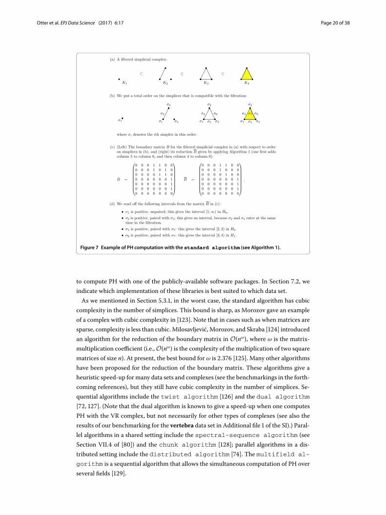
Figure 7 Example of PH computation with the standard algorithm (see Algorithm 1).

to compute PH with one of the publicly-available software packages. In Section ., weindicate which implementation of these libraries is best suited to which data set.

As we mentioned in Section .., in the worst case, the standard algorithm has cubiccomplexity in the number of simplices. This bound is sharp, as Morozov gave an exampleof a complex with cubic complexity in []. Note that in cases such as when matrices aresparse, complexity is less than cubic. Milosavljević, Morozov, and Skraba [] introducedan algorithm for the reduction of the boundary matrix in O(nω), where ω is the matrix-multiplication coefficient (i.e., O(nω) is the complexity of the multiplication of two squarematrices of size n). At present, the best bound for ω is . []. Many other algorithmshave been proposed for the reduction of the boundary matrix. These algorithms give aheuristic speed-up for many data sets and complexes (see the benchmarkings in the forth-coming references), but they still have cubic complexity in the number of simplices. Se-quential algorithms include the twist algorithm [] and the dual algorithm

[, ]. (Note that the dual algorithm is known to give a speed-up when one computesPH with the VR complex, but not necessarily for other types of complexes (see also theresults of our benchmarking for the vertebra data set in Additional file of the SI).) Paral-lel algorithms in a shared setting include the spectral-sequence algorithm (seeSection VII. of []) and the chunk algorithm []; parallel algorithms in a dis-tributed setting include the distributed algorithm []. The multifield al-

gorithm is a sequential algorithm that allows the simultaneous computation of PH overseveral fields [].


5.4 Statistical interpretation of topological summariesOnce one has obtained barcodes, one needs to interpret the results of computations. Inapplications, one often wants to compare the output of a computation for a certain dataset with the output for a null model. Alternatively, one may be studying data sets from theoutput of a generative model (e.g., many realizations from a model of random networks),and it is then necessary to average results over multiple realizations. In the first instance,one needs both a way to compare the two different outputs and a way to evaluate thesignificance of the result for the original data set. In the second case, one needs a way tocalculate appropriate averages (e.g., summary statistics) of the result of the computations.

From a statistical perspective, one can interpret a barcode as an unknown quantity thatone tries to estimate by computing PH. If one wants to use PH in applications, one thusneeds a reliable way to apply statistical methods to the output of the computation of PH.To our knowledge, statistical methods for PH were addressed for the first time in the pa-per []. Roughly speaking, there are three current approaches to the problem of sta-tistical analysis of barcodes. In the first approach, researchers study topological proper-ties of random simplicial complexes (see, e.g., [, ]) and the review papers [, ].One can view random simplicial complexes as null models to compare with empirical datawhen studying PH. In the second approach, one studies properties of a metric space whosepoints are persistence diagrams. In the third approach, one studies ‘features’ of persistencediagrams. We will provide a bit more detail about the second and third approaches.

In the second approach, one considers an appropriately defined ‘space of persistencediagrams,’ defines a distance function on it, studies geometric properties of this space,and does standard statistical calculations (means, medians, statistical tests, and so on).Recall that a persistence diagram (see Figure for an example) is a multiset of points inR and that it gives the same information as a barcode. We now give the following precisedefinition of a persistence diagram.

Definition A persistence diagram is a multiset that is the union of a finite multiset ofpoints in R with the multiset of points on the diagonal ) = {(x, y) ∈ R | x = y}, whereeach point on the diagonal has infinite multiplicity.

In this definition, we include all of the points on the diagonal in R with infinite mul-tiplicity for technical reasons. Roughly, it is desirable to be able to compare persistencediagrams by studying bijections between their elements, and persistence diagrams mustthus be sets with the same cardinality.

Given two persistence diagrams X and Y , we consider the following general definitionof distance between X and Y .

Definition Let p ∈ [,∞]. The pth Wasserstein distance between X and Y is defined as

Wp[d](X, Y ) := infφ:X→Y

*!

x∈Xd%x,φ(x)

&p+/p

for p ∈ [,∞) and as

W∞[d](X, Y ) := infφ:X→Y

supx∈X

d%x,φ(x)

&

for p = ∞, where d is a metric on R and φ ranges over all bijections from X to Y .


Usually, one takes d = Lq for q ∈ [,∞]. One of the most commonly employed distancefunctions is the bottleneck distance W∞[L∞].

The development of statistical analysis on the space of persistence diagrams is an areaof ongoing research, and presently there are few tools that can be used in applications. See[–] for research in this direction. Until recently, the library DIONYSUS [] was theonly library to implement computation of the bottleneck and Wasserstein distances (ford = L∞); the library HERA [] implements a new algorithm [] for the computation ofthe bottleneck and Wasserstein distances that significantly outperforms the implementa-tion in DIONYSUS. The library TDA PACKAGE [] (see [] for the accompanying tu-torial) implements the computation of confidence sets for persistence diagrams that wasdeveloped in [], distance functions that are robust to noise and outliers [], and manymore tools for interpreting barcodes.

The third approach for the development of statistical tools for PH consists of mappingthe space of persistence diagrams to spaces (e.g., Banach spaces) that are amenable tostatistical analysis and machine-learning techniques. Such methods include persistencelandscapes [], using the space of algebraic functions [], persistence images [],and kernelization techniques [–]. See the papers [, ] for applications of persis-tence landscapes. The package PERSISTENCE LANDSCAPE TOOLBOX [] (see [] for theaccompanying tutorial) implements the computation of persistence landscapes, as well asmany statistical tools that one can apply to persistence landscapes, such as mean, ANOVA,hypothesis tests, and many more.

5.5 StabilityAs we mentioned in Section , PH is useful for applications because it is stable with respectto small perturbations in the input data.

The first stability theorem for PH, proven in [], asserts that, under favorable condi-tions, step () in the pipeline in Figure is -Lipschitz with respect to suitable distancefunctions on filtered complexes and the bottleneck distance for barcodes (see Section .).This result was generalized in the papers [–]. Stability for PH is an active area ofresearch; for an overview of stability results, their history and recent developments, see[], Chapter .

6 Excursus: generalized persistenceOne can use the algorithms that we described in Section to compute PH when one hasa sequence of complexes with inclusion maps that are all going in the same direction, asin the following diagram:

· · · → Ki– → Ki → Ki+ → · · · .

An algorithm, called the zigzag algorithm, for the computation of PH for inclusionmaps that do not all go in the same direction, as, e.g., in the diagram

· · · → Ki– → Ki ← Ki+ → · · ·

was introduced in []. In the more general setting in which maps are not inclusions, onecan still compute PH using the simplicial map algorithm [].


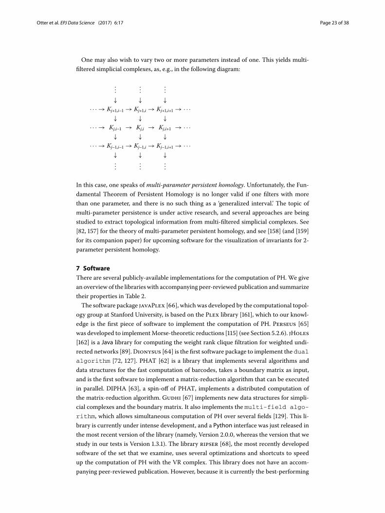
One may also wish to vary two or more parameters instead of one. This yields multi-filtered simplicial complexes, as, e.g., in the following diagram:

......

...↓ ↓ ↓

· · · → Kj+,i– → Kj+,i → Kj+,i+ → · · ·↓ ↓ ↓

· · · → Kj,i– → Kj,i → Kj,i+ → · · ·↓ ↓ ↓

· · · → Kj–,i– → Kj–,i → Kj–,i+ → · · ·↓ ↓ ↓...

......

In this case, one speaks of multi-parameter persistent homology. Unfortunately, the Fun-damental Theorem of Persistent Homology is no longer valid if one filters with morethan one parameter, and there is no such thing as a ‘generalized interval.’ The topic ofmulti-parameter persistence is under active research, and several approaches are beingstudied to extract topological information from multi-filtered simplicial complexes. See[, ] for the theory of multi-parameter persistent homology, and see [] (and []for its companion paper) for upcoming software for the visualization of invariants for -parameter persistent homology.

7 SoftwareThere are several publicly-available implementations for the computation of PH. We givean overview of the libraries with accompanying peer-reviewed publication and summarizetheir properties in Table .

The software package JAVAPLEX [], which was developed by the computational topol-ogy group at Stanford University, is based on the PLEX library [], which to our knowl-edge is the first piece of software to implement the computation of PH. PERSEUS []was developed to implement Morse-theoretic reductions [] (see Section ..). JHOLES[] is a Java library for computing the weight rank clique filtration for weighted undi-rected networks []. DIONYSUS [] is the first software package to implement the dualalgorithm [, ]. PHAT [] is a library that implements several algorithms anddata structures for the fast computation of barcodes, takes a boundary matrix as input,and is the first software to implement a matrix-reduction algorithm that can be executedin parallel. DIPHA [], a spin-off of PHAT, implements a distributed computation ofthe matrix-reduction algorithm. GUDHI [] implements new data structures for simpli-cial complexes and the boundary matrix. It also implements the multi-field algo-

rithm, which allows simultaneous computation of PH over several fields []. This li-brary is currently under intense development, and a Python interface was just released inthe most recent version of the library (namely, Version .., whereas the version that westudy in our tests is Version ..). The library RIPSER [], the most recently developedsoftware of the set that we examine, uses several optimizations and shortcuts to speedup the computation of PH with the VR complex. This library does not have an accom-panying peer-reviewed publication. However, because it is currently the best-performing


Tabl

e2

Ove

rvie

wof

exis

ting

soft

war

efo

rthe

com

puta

tion

ofPH

that

have

anac

com

pany

ing

peer

-rev

iew

edpu

blic

atio

n(a

ndal

soRI

PSER

[68]

,bec

ause

ofits

perf

orm

ance

)

Soft

war

eJA

VAPL

EXPE

RSEU

SJH

OLE

SD

ION

YSU

SPH

ATD

IPH

AG

UD

HI

SIM

PPER

SRI

PSER

(a)L

angu

age

Java

C++

Java

C++

C++

C++

C++

C++

C++

(b)A

lgor

ithm

sfor

PHst

anda

rd,d

ual,

zigz

agM

orse

redu

ctio

ns,

stan

dard

stan

dard

(use

sJA

VAPL

EX)

stan

dard

,dua

l,zig

zag

stan

dard

,dua

l,tw

ist,c

hunk

,sp

ectr

alse

quen

ce

twist

,dua

l,di

strib

uted

dual

,mul

tifiel

dsim

plic

ialm

aptw

ist,d

ual

(c)C

oeffi

cien

tfiel

dQ

,Fp

F 2F 2

F 2(s

tand

ard,

zigz

ag),

F p(d

ual)

F 2F 2

F pF 2

F p

(d)H

omol

ogy

simpl

icia

l,cel

lula

rsim

plic

ial,c

ubic

alsim

plic

ial

simpl

icia

lsim

plic

ial,c

ubic

alsim

plic

ial,c

ubic

alsim

plic

ial,c

ubic

alsim

plic

ial

simpl

icia

l(e

)Filt

ratio

nsco

mpu

ted

VR,W

,Wν

VR,l

ower

star

ofcu

bica

lcom

plex

WRC

FVR

,α,C

-VR

,low

erst

arof

cubi

calc

ompl

exVR

,α,W

,low

erst

arof

cubi

cal

com

plex

-VR

(f)F

iltra

tions

asin

put

simpl

icia

lco

mpl

ex,z

igza

g,CW

simpl

icia

lco

mpl

ex,c

ubic

alco

mpl

ex

-sim

plic

ialc

ompl

ex,

zigz

agbo

unda

rym

atrix

ofsim

plic

ialc

ompl

exbo

unda

rym

atrix

ofsim

plic

ial

com

plex

-m

apof

simpl

icia

lco

mpl

exes

-

(g)A

dditi

onal

feat

ures

Com

pute

ssom

eho

mol

ogic

alal

gebr

aco

nstr

uctio

ns,

hom

olog

yge

nera

tors

wei

ghte

dpo

ints

forV

R-

vine

yard

s,ci

rcle

-val

ued

func

tions

,hom

olog

yge

nera

tors

--

--

-

(h)V

isual

izat

ion

barc

odes

pers

isten

cedi

agra

m-

--

pers

isten

cedi

agra

m-

--

The

sym

bol‘

-’sig

nifie

stha

tthe

asso

ciat

edfe

atur

eis

noti

mpl

emen

ted.

Fore

ach

soft

war

epa

ckag

e,w

ein

dica

teth

efo

llow

ing

item

s.(a

)The

lang

uage

inw

hich

itis

impl

emen

ted.

(b)T

heim

plem

ente

dal

gorit

hmsf

orth

eco

mpu

tatio

nof

barc

odes

from

the

boun

dary

mat

rix.(

c)Th

eco

effic

ient

field

sfor

whi

chPH

isco

mpu

ted,

whe

reth

ele

tter

pde

note

sany

prim

enu

mbe

rin

the

coef

ficie

ntfie

ldF p

.(d)

The

type

ofho

mol

ogy

com

pute

d.(e

)The

filte

red

com

plex

esth

atar

eco

mpu

ted,

whe

reVR

stan

dsfo

rVie

toris

–Rip

scom

plex

, Wst

ands

fort

hew

eak

witn

essc

ompl

ex,W

νst

ands

forp

aram

etriz

edw

itnes

scom

plex

es,W

RCF

stan

dsfo

rthe

wei

ghtr

ank

cliq

uefil

trat

ion,

α

stan

dsfo

rthe

alph

aco

mpl

ex,a

ndC

fort

heCe

chco

mpl

ex.P

ERSE

US,

DIP

HA

,and

GU

DH

Iim

plem

entt

heco

mpu

tatio

nof

the

low

er-s

tarfi

ltrat

ion

[160

]ofa

wei

ghte

dcu

bica

lcom

plex

;one

inpu

tsda

tain

the

form

ofa

d-di

men

siona

larr

ay;t

heda

tais

then

inte

rpre

ted

asa

d-di

men

siona

lcub

ical

com

plex

,and

itslo

wer

-sta

rfiltr

atio

nis

com

pute

d.(S

eeth

eTu

toria

lin

Addi

tiona

lfile

2of

the

SI,f

orm

ore

deta

ils.)

Not

eth

atD

IPH

Aan

dG

UD

HIu

seth

eef

ficie

ntre

pres

enta

tion

ofcu

bica

lcom

plex

espr

esen

ted

in[5

5],s

oth

esiz

eof

the

cubi

calc

ompl

exth

atis

com

pute

dby

thes

elib

rarie

siss

mal

lert

han

the

size

ofth

ere

sulti

ngco

mpl

exw

ithPE

RSEU

S.(f

)The

filte

red

com

plex

esth

aton

eca

ngi

veas

inpu

t.JA

VAPL

EXsu

ppor

tsth

ein

puto

fafil

tere

dCW

com

plex

fort

heco

mpu

tatio

nof

cellu

larh

omol

ogy

[78]

;in

cont

rast

with

simpl

icia

lcom

plex

es,t

here

dono

tcur

rent

lyex

istal

gorit

hmst

oas

sign

ace

llco

mpl

exto

poin

t-cl

oud

data

.(g)

Addi

tiona

lfea

ture

sim

plem

ente

dby

the

libra

ry. J

AVA

PLEX

supp

orts

the

com

puta

tion

ofso

me

cons

truc

tions

from

hom

olog

ical

alge

bra

(see

[66]

ford

etai

ls),a

ndPE

RSEU

Sim

plem

ents

the

com

puta

tion

ofPH

with

the

VRfo

rpoi

ntsw

ithdi

ffere

nt‘b

irth

times

’(se

eSe

ctio

n5.

1.3)

.The

libra

ryD

ION

YSU

Sim

plem

ents

the

com

puta

tion

ofvi

neya

rds[

155]

and

circ

le-v

alue

dfu

nctio

ns[1

27].

Both

JAVA

PLEX

and

DIO

NYS

US

supp

ortt

heou

tput

ofre

pres

enta

tives

ofho

mol

ogy

clas

sesf

orth

ein

terv

alsi

na

barc

ode.

(h)W

heth

ervi

sual

izat

ion

ofth

eou

tput

ispr

ovid

ed


(both in terms of memory usage and in terms of wall-time secondsh) library for the com-putation of PH with the VR complex, we include it in our study. The library SIMPPERS[] implements the simplicial map algorithm. Libraries that implement tech-niques for the statistical interpretation of barcodes include the TDA PACKAGE [] andthe PERSISTENCE LANDSCAPE TOOLBOX []. (See Section . for additional libraries forthe interpretation of barcodes.) RIVET, a package for visualizing -parameter persistenthomology, is slated to be released soon []. We summarize the properties of the librariesfor the computation of PH that we mentioned in this paragraph in Table , and we discussthe performance for a selection of them in Section .. and in Additional file of the SI.For a list of programs, see https://github.com/n-otter/PH-roadmap.

7.1 BenchmarkingWe benchmark a subset of the currently available open-source libraries with peer-reviewed publication for the computation of PH. To our knowledge, the published open-source libraries are JHOLES, JAVAPLEX, PERSEUS, DIONYSUS, PHAT, DIPHA, SIMPPERS,and GUDHI. To these, we add the library RIPSER, which is currently the best-performinglibrary to compute PH with the VR complex. To study the performance of the packages,we restrict our attention to the algorithms that are implemented by the largest numberof libraries. These are the VR complex and the standard and dual algorithms for the re-duction of the boundary matrix. PHAT only takes a boundary matrix as input, so it is notpossible to conduct a direct comparison of it with the other implementations. However,the fast data structures and algorithms implemented in PHAT are also implemented in itsspin-off software DIPHA, which we include in the benchmarking. The software JHOLEScomputes PH using the WRCF for weighted undirected networks, and SIMPPERS takes amap of simplicial complexes as input, so these two libraries cannot be compared directlyto the other libraries. In Additional file of the SI, we report benchmarking of some addi-tional features that are implemented by some of the six libraries (i.e., JAVAPLEX, PERSEUS,DIONYSUS, DIPHA, GUDHI, and RIPSER) that we test. Specifically, we report results forthe computation of PH with cubical complexes for image data sets and the computationof PH with witness, alpha, and Čech complexes.

We study the software packages JAVAPLEX, PERSEUS, DIONYSUS, DIPHA, GUDHI, andRIPSER using both synthetic and real-world data from three different perspectives:

. Performance measured in CPU seconds and wall-time (i.e., elapsed time) seconds.. Memory required by the process.. Maximum size of simplicial complex allowed by the software.

.. Data setsIn this subsection, we describe the data sets that we use for our benchmarking. We usedata sets from a variety of different mathematical and scientific areas and applications. Ineach case, when possible, we use data sets that have already been studied using PH. Ourlist of data sets is far from complete; we view this list as an initial step towards building acomprehensive collection of benchmarking data sets for PH.

Data sets ()–() are synthetic; they arise from topology (), stochastic topology (),dynamical systems (), and from an area at the intersection of network theory and fractalgeometry (). (As we discuss below, data set () was used originally to study connectionpatterns in the cerebral cortex.) Data sets ()–() are from empirical experiments and


Figure 8 Two well-known examples. (a) Plot ofthe image of the figure-8 immersion of the Kleinbottle and (b) the reconstruction of the StanfordDragon (retrieved from [164]).

measurements: they arise from phylogenetics ()–(), image analysis (), genomics (),neuroscience (), medical imaging (), political science (), and scientometrics ().

In each case, these data sets are of one of the following three types: point clouds,weighted undirected networks, and gray-scale digital images. To obtain a point cloud froma real-world weighted undirected network, we compute shortest paths using the inverseof the nonzero weights of edges as distances between nodes (except for the US Congressnetworks and the human genome network; see below). For the synthetic networks, thevalues assigned to edges are interpreted as distances between nodes, and we therefore usethese values to compute shortest paths. We make all processed versions of the data setsthat we use in the benchmarking available at https://github.com/n-otter/PH-roadmap/tree/master/data_sets. We provide the scripts that we used to produce the synthetic datasets at https://github.com/n-otter/PH-roadmap/tree/master/matlab/synthetic_data_sets_scripts.

We now describe all data sets in detail:() Klein bottle. The Klein bottle is a one-sided nonorientable surface (see Figure ).

We linearly sample points from the Klein bottle using its ‘figure-’ immersion in R

and size sample of points. We denote this data set by Klein. Note that theimage of the immersion of the Klein bottle does not have the same homotopy typeas the original Klein bottle, but it does have the same singular homologyi withcoefficients in F. We have H(B) = F, H(B) = F ⊕ F, and H(B) = F, where Bdenotes the Klein bottle and Hi(B) is the ith singular homology group withcoefficients in F.

() Random VR complexes (uniform distribution) []. The parameters for thismodel are positive integers N and d; the random VR complex for parameters Nand d is the VR complex VRϵ(X), where X is a set of N points sampled from Rd .(Equivalently, the random VR complex is the clique complex on the randomgeometric graph G(N , ϵ) [].) We sample N points uniformly at random from[, ]d . We choose (N , d) = (, ) and we denote this data set by random. Thehomology of random VR complexes was studied in [].

() Vicsek biological aggregation model. This model was first introduced in [] andwas studied using PH in []. We implement the model in the form in which itappears in []. The model describes the motion of a collection of particles thatinteract in a square with periodic boundary conditions. The parameters for themodel are the length l of the side of the square, the initial angle θ, the (constant)absolute value v for the velocity, the number N of particles, a noise parameter η,and the number T of time steps. The output of the model is a point cloud in-dimensional Euclidean space in which each point is specified by its position inthe -dimensional box and its velocity angle (‘heading’). We run three simulationsof the model using the parameter values from []. For each simulation, we choose


two point clouds that correspond to two different time frames. See [] for furtherdetails. We denote this data set by Vicsek.

() Fractal networks. These are self-similar networks introduced in [] to investigatewhether connection patterns of the cerebral cortex are arranged in self-similarpatterns. The parameters for this model are natural numbers b, k, and n. Togenerate a fractal network, one starts with a fully-connected network with b

nodes. Two copies of this network are connected to each other so that the‘connection density’ between them is k–, where the connection density is thenumber of edges between the two copies divided by the number of total possibleedges between them. Two copies of the resulting network are connected withconnection density k–. One repeats this type of connection process until thenetwork has size n, but with a decrease in the connection density by a factor of /kat each step.

We define distances between nodes in two different ways: () uniformly atrandom, and () with linear weight-degree correlations. In the latter, the distancebetween nodes i and j is distributed as kikjX , where ki is the degree of node i and Xis a random variable uniformly distributed on the unit interval. We use theparameters b = , n = , and k = ; and we compute PH for the weighted networkand for the network in which all adjacent nodes have distance . We denote thisdata set by fract and distinguish between the two ways of defining distancesbetween weights using the abbreviations ‘r’ for random, and ‘l’ for linear.

() Genomic sequences of the HIV virus. We construct a finite metric space using theindependent and concatenated sequences of the three largest genes — gag, pol,and env — of the HIV genome. We take , different genomic sequences andcompute distances between them by using the Hamming distance. We use thealigned sequences studied using PH in []. (The authors of that paper retrievedthe sequences from [].) We denote this data set by HIV.

() Genomic sequences of HN. This data set consists of , different genomicsequences of HN influenza. We compute the Hamming distance betweensequences. We use the aligned sequences studied using PH in []. We denote thisdata set by HN.

() Stanford Dragon graphic. We sample points uniformly at random from-dimensional scans of the dragon [], whose reconstruction we show inFigure . The sample sizes include , and , points. We denote these datasets by drag and drag , respectively.

() C. elegans neuronal network. This is a weighted, undirected network in which eachnode is a neuron and edges represent synapses or gap junctions. We use thenetwork studied using PH in []. (The authors of the paper used the data setstudied in [], which first appeared in [].) Recall that for this example, and alsofor the other real-world weighted networks (except for the human genome networkand the US Congress networks), we convert each nonzero edge weight to adistance by taking its inverse. We denote this data set by eleg.

() Human genome. This is a weighted, undirected network representing a sample ofthe human genome. We use the network studied using PH in []. (The authors ofthat paper created the sample using data retrieved from [].) Each noderepresents a gene, and two nodes are adjacent if there is a nonzero correlation


between the expression levels of the corresponding genes. We define the weight ofan edge as the inverse of the correlation.j We denote this data set by genome.

() Gray-scale image: -dimensional rotational angiography scan of a head with ananeurysm. This data set was used in the benchmarking in []. This data set isgiven by a -dimensional array of size × × , where each entry stores aninteger that represents the grey value for the corresponding voxel. We retrieved thedata set from the repository []. We denote this data set by vertebra.

() US Congress roll-call voting networks. These two networks (the Senate and Houseof Representatives from the th United States Congress) are constructed usingthe procedure in [] from data compiled by []. In each network, a node is alegislator (Senators in one data set and Representatives in the other), and there is aweighted edge between legislators i and j, where the weight wi,j is a number in [, ](it is equal to if and only if legislators i and j never voted the same way on anybill) given by the number of times the two legislators voted in the same way dividedby the total number of bills on which they both voted. See [] for further details.We denote the networks from the Senate and House by senate and house,respectively. The network senate has nodes, and the network house has nodes. To compute shortest paths, we define the distance between two nodes i andj to be – wi,j. In the th Congress, no two politicians voted in the same way onevery bill, so we do not have distinct nodes with distance between them. (This isimportant, for example, if one wants to apply multidimensional scaling.)

() Network of network scientists. This is a weighted, undirected networkrepresenting the largest connected component of a collaboration network ofnetwork scientists []. Nodes represent authors and edges representcollaborations, and weights indicate the number of joint papers. The largestconnected component consists of nodes. We denote this data set by netw-sc.

.. Machines and compilersWe tested the libraries on both a cluster and a shared-memory system. The cluster is a DellSandybridge cluster, it has , (i.e., × ) cores of . GHz Xeon SandyBridge, RAMof GiB in nodes and RAM of GiB in nodes, and a scratch disk of TB. It runsthe operating system (OS) Red Hat Enterprise Linux . The shared-memory system is anIBM System x M server with (i.e., × ) cores of . GHz, RAM of GB, andstorage of TB. It runs the OS Ubuntu ...k The major difference in running sharedalgorithms on the shared-memory system versus the distributed-memory system is thateach node in the former has much more available RAM than in the latter. (See also thedifference in performance between computations on cluster and shared memory systemin Tables and .) To compile GUDHI, DIPHA, PERSEUS, and DIONYSUS, we used thecompiler gcc .. on the cluster and gcc .. on the shared-memory system; for bothmachines, we used the (default) optimization -O3. Additionally, we used openmpi ..for DIPHA.

.. Tests and resultsWe now report the details and results of the tests that we performed. We have madethe data sets, header file to measure memory, and other information related to the testsavailable at https://github.com/n-otter/PH-roadmap. Of the six software packages that


Table 3 Performance of the software packages measured in wall-time (i.e., elapsed time), andCPU seconds (for the computations running on the cluster)

Data set (a) Computations on cluster: wall-time seconds

eleg Klein HIV drag 2 random genome

Size of complex 4.4 × 106 1.1 × 107 2.1 × 108 1.3 × 109 3.1 × 109 4.5 × 108

Max. dim. 2 2 2 2 8 2JAVAPLEX (st) 84 747 - - - -DIONYSUS (st) 474 1,830 - - - -DIPHA (st) 6 90 1,631 142,559 - 9,110PERSEUS 543 1,978 - - - -DIONYSUS (d) 513 145 - - - -DIPHA (d) 4 6 81 2,358 5,096 232GUDHI 36 89 1,798 14,368 - 4,753RIPSER 1 1 2 6 349 3

Data set (b) Computations on cluster: CPU seconds


Size of complex 4.4 × 106 1.1 × 107 2.1 × 108 1.3 × 109 3.1 × 109 4.5 × 108

Max. dim. 2 2 2 2 8 2JAVAPLEX (st) 284 1,031 - - - -DIONYSUS (st) 473 1,824 - - - -DIPHA (st) 68 1,360 25,950 1,489,615 - 130,972PERSEUS 542 1,974 - - - -DIONYSUS (d) 513 145 - - - -DIPHA (d) 39 73 1,276 37,572 79,691 3,622GUDHI 36 88 1,794 14,351 - 4,764RIPSER 1 1 2 5 348 2

Data set (c) Computations on shared-memory system: wall-time seconds

eleg Klein HIV drag 2 genome fract r

Size of complex 3.2 × 108 1.1 × 107 2.1 × 108 1.3 × 109 4.5 × 108 2.8 × 109

Max. dim. 3 2 2 2 2 3JAVAPLEX (st) 13,607 1,358 43,861 - 28,064 -PERSEUS - 1,271 - - - -DIONYSUS (d) - 100 142,055 35,366 - 572,764DIPHA (d) 926 13 773 4,482 1,775 3,923GUDHI 381 6 177 1,518 442 4,590RIPSER 2 1 2 5 3 1,517

For each data set, we indicate the size of the simplicial complex and the maximum dimension up to which we construct theVR complex. For all data sets, we construct the filtered VR complex up to the maximum distance between any two points. Weindicate the implementation of the standard algorithm using the abbreviation ‘st’ following the name of the package, andwe indicate the implementation of the dual algorithm using the abbreviation ‘d.’ The symbol ‘-’ signifies that we were unableto finish computations for this data set, because the machine ran out of memory. PERSEUS implements only the standardalgorithm, and GUDHI and RIPSER implement only the dual algorithm. (a), (b) We run DIPHA on one node and 16 cores for thedata sets eleg, Klein, and genome; on 2 nodes of 16 cores for the HIV data set; on 2 and 3 nodes of 16 cores for the dual andstandard implementations, respectively, for drag 2; and on 8 nodes of 16 cores for random. (The maximum number ofprocesses that we could use at any one time was 128.) (c) We run DIPHA on a single core.

we study, four implement the computation of the dual algorithm, and four implement thestandard algorithm. It is reported in [] that JAVAPLEX implements the dual algorithm,but the implementation of the algorithm has a bug and gives a wrong output. To our knowl-edge, this bug has not yet been fixed (at the time of writing), and we therefore test onlythe standard algorithm.

For the computations on the cluster, we compare the libraries running both the dualalgorithm and the standard algorithm. The package DIPHA is the only one to implementa distributed computation. As a default, we run the software on one node and cores;we only increase the number of nodes and cores employed when the machine runs out ofmemory. However, augmenting the number of nodes can make the computations faster


Table 4 Memory usage in GB for the computations summarized in Table 3

Data set (a) Computations on cluster


Size of complex 4.4 × 106 1.1 × 107 2.1 × 108 1.3 × 109 3.1 × 109 4.5 × 108

Max. dim. 2 2 2 2 8 2JAVAPLEX (st) <5 <15 >64 >64 >64 >64DIONYSUS (st) 1.3 11.6 - - - -DIPHA (st) 0.1 0.2 2.7 4.9 - 4.8PERSEUS 5.1 12.7 - - - -DIONYSUS (d) 0.5 1.1 - - - -DIPHA (d) 0.1 0.2 1.8 13.8 9.6 6.3GUDHI 0.2 0.5 8.5 62.8 - 21.5RIPSER 0.007 0.02 0.06 0.2 24.7 0.07

Data set (b) Computations on shared-memory system

eleg Klein HIV drag 2 genome fract r

Size of complex 3.2 × 108 1.1 × 107 2.1 × 108 1.3 × 109 4.5 × 108 2.8 × 109

Max. dim. 3 2 2 2 2 3JAVAPLEX (st) <600 <15 <700 >700 <700 >700PERSEUS - 11.7 - - - -DIONYSUS (d) - 1.1 16.8 134.2 - 268.5DIPHA (d) 31.2 0.9 17.7 109.5 37.3 276.1GUDHI 15.4 0.5 10.2 62.8 21.4 134.8RIPSER 0.2 0.03 0.07 0.2 0.07 155

For JAVAPLEX, we indicate the value of the maximum heap size that was sufficient to perform the computation. The valuethat we give is an upper bound to the memory usage. For DIPHA, we indicate the maximum memory used by a single core(considering all cores). See Table 3 for details on the number of cores used.

(in terms of CPU seconds) for complexes of all sizes.l We see this in our experiments, andit is also discussed in []. For the other packages, we run the computations on a singlenode with one core.

For computations on the shared-memory system, we compare the libraries using onlythe dual algorithm if they implement it, and we otherwise use the standard algorithm. Forthe shared-memory system, we run all packages (including DIPHA) on a single core.

In our benchmarking, we report mean computation times and memory measurements.In Table , we give the computation times for the different software packages. We mea-sure elapsed and CPU time by using the time function in Linux. We report computa-tion times with a precision of one second; if a computation took only fractions of a sec-ond, we report ‘one second’ as the computation time. For space reasons, we report resultsfor a subset of the computations. (In Additional file of the SI, we tabulate the rest ofour computations.) In Table , we report the memory used by the processes in terms ofmaximum resident set size (RSS); in other words, we give the maximum amount of realRAM a program has used during its execution. We measure the maximum RSS using thegetrusage function in Linux. The header file that we use to measure memory is avail-able at https://github.com/n-otter/PH-roadmap. In DIPHA, the measurement of mem-ory is already implemented by the authors of the software. They also use the getrusagefunction in Linux. The package JAVAPLEX is written in Java, and we thus cannot measureits memory as we do for the other packages. However, one can infer memory requirementsfor this software package using the value of the maximal heap size necessary to performthe computations; we report this value in Table . In Table , we give the maximum size ofthe simplicial complex for which we were able to compute PH with each software packagein our benchmarkings.


Table 5 For each software package in (a), we indicate in (b) the maximal size of the simplicialcomplex supported by it thus far in our tests

(a) JAVAPLEX DIONYSUS DIPHA PERSEUS GUDHI RIPSERst st d st d st d d

(b) 4.5 · 108 1.1 · 107 2.8 × 109 1.3 · 109 3.4 · 109 1 · 107 3.4 · 109 3.4 · 109

7.2 Conclusions from our benchmarkingOur tests suggest that RIPSER is the best-performing library currently available for thecomputation of PH with the Vietoris–Rips complex, and in order of decreasing perfor-mance, that GUDHI and DIPHA are the next-best implementations. For the computationof PH with cubical complexes, GUDHI outperforms DIPHA by a factor of to in termsof memory usage, and DIPHA outperforms GUDHI in terms of wall-time seconds by a fac-tor of to (when running on one core on a shared-memory system). Both DIPHA andGUDHI significantly outperform the implementation in PERSEUS. For the computation ofPH with the alpha complex, we did not observe any significant differences in performancebetween the libraries GUDHI and DIONYSUS. Because the alpha complex has fewer sim-plices than the other complexes that we used in our tests, further tests with larger datasets may be appropriate in future benchmarkings.

There is a huge disparity between implementations of the dual and standard algorithmswhen computing PH with the VR complex. In our benchmarking, the dual implementa-tions outperformed standard ones both in terms of computation time (with respect to bothCPU and wall-time seconds) and in terms of the amount of memory used. This significantdifference in performance and memory usage was also revealed for the software packageDIONYSUS in []. However, note that when computing PH for other types of complexes,the standard algorithm may be better suited than the dual algorithm. (See, e.g., the resultof our test for the vertebra data set in Additional file of the SI.)

To conclude, in our benchmarking, the fastest software packages were RIPSER, GUDHI,and DIPHA. For small complexes, the software packages PERSEUS and JAVAPLEX are goodchoices, because they are the easiest ones to use. (They are the only libraries that need onlyto be downloaded and are then ‘plug-and-play,’ and they have user-friendly interfaces.)Because the library JAVAPLEX implements the computation of a variety of complexes andalgorithms, we feel that it is the best software for an initial foray into PH computation.

We now give guidelines for the computation of PH based on our benchmarking. We listseveral types of data sets in Table and indicate which software or algorithm that we feel isbest-suited to each one. These guidelines are based on the findings of our benchmarking.Note that one can transform networks into distance matrices, and distance matrices canyield points in Euclidean space using a method such as multi-dimensional scaling. Natu-rally, given a finite set of points in Euclidean space, we can compute their distance matrix.As we discussed in Section ., image data can also be considered as a finite metric space,so the indications for distance matrices and points in Euclidean space also apply to imagedata.

8 Future directionsWe conclude by discussing some future directions for the computation of PH. As we sawin Section , much work has been done on step (i.e., going from filtered complexes tobarcodes) of the PH pipeline of Figure , and there exist implementations of many fast


Table 6 Guidelines for which implementation is best-suited for which data set, based on ourbenchmarking

Data type Complex Suggested software

networks WRCF JHOLES

image data cubical GUDHI or DIPHA (st)distance matrix VR RIPSER

distance matrix W JAVAPLEX

points in Euclidean space VR GUDHI

points in Euclidean space C DIONYSUS

points in Euclidean space α (only in dim 2 and 3) DIONYSUS ((st) in dim 2, (d) in dim 3) or GUDHI

Recall that we indicate the implementation of the dual algorithm using the abbreviation ‘d’ following the name of a package,and similarly we indicate the implementation of the standard algorithm by ‘st’. Note that for smaller data sets one can alsouse JAVAPLEX to compute PH with VR complexes from points in Euclidean space, and PERSEUS to compute PH with cubicalcomplexes for image data, and with VR complexes for distance matrices. The library JHOLES can only handle networks withdensity much less than 1.

algorithms for the reduction of the boundary matrix. Step (i.e., going from data to a fil-tered complex) of the PH pipeline is an active area of research, but many sparsificationtechniques (see, e.g., [, ]) for complexes have yet to be implemented, and more re-search needs to be done on steps and (i.e., interpreting barcodes; see, e.g., [, ,]) of the PH pipeline. In particular, it is important to develop approaches for statisticalanalysis of persistent homology.

We believe that there needs to be a community-wide effort to build a library that imple-ments the algorithms and data structures for the computation of PH, and that it should bedone in a way that new algorithms and methods can be implemented easily in this frame-work. This would parallel similar community-wide efforts in fields such as computationalalgebra and computational geometry, and libraries such as Macaulay [], Sage [],and CGAL [].

We also believe that there is a need to create guidelines and benchmark data sets for thetest of new algorithms and data structures. The methods and collection of data sets thatwe used in our benchmarking provide an initial step towards establishing such guidelinesand a list of test problems.

9 List of abbreviations. α: alpha complex. d (following the name of a library): implementation of the dual algorithm. Č: Čech complex. PH: persistent homology. SI: Supplementary Information. st (following the name of a library): implementation of the standard algorithm. TDA: topological data analysis. VR: Vietoris–Rips complex. W: weak witness complex

. Wν : parametrized witness complexes. WRCF: weight rank clique filtration

10 Availability of data and materialsThe processed version of the data sets used in the benchmarking and the scripts writtenfor the tutorial are available at https://github.com/n-otter/PH-roadmap. The open-source


libraries for the computation of PH studied in this paper are available at the referencesindicated in the associated citations.

Additional material

Additional file 1: Additional computations. (pdf )Additional file 2: Tutorial for ‘A roadmap for the computation of persistent homology’. (pdf )

AcknowledgementsWe thank the Rabadan Lab at Columbia University for providing the HIV and H3N2 sequences used in [23] and GiovanniPetri for sharing the data sets used in [89]. We thank Krishna Bhogaonker, Adrian Clough, Patrizio Frosini, Florian Klimm,Yacoub Kureh, Vitaliy Kurlin, Robert MacKay, James Meiss, Dane Taylor, Leo Speidel, Parker Edwards, and Bernadette Stolzfor helpful comments on a draft of this paper. We also thank the anonymous referees for their many helpful comments.The first author thanks Ulrich Bauer, Michael Lesnick, Hubert Wagner, and Matthew Wright for helpful discussions, andthanks Florian Klimm, Vidit Nanda, and Bernadette Stolz for precious advice. The authors would like to acknowledge theuse of the University of Oxford Advanced Research Computing (ARC) facility (http://dx.doi.org/10.5281/zenodo.22558) incarrying out some of the computations performed in this work. The first author thanks the support team at the ARC fortheir assistance. NO and PG are grateful for support from the EPSRC grant EP/G065802/1 (The Digital Economy HORIZONHub). HAH gratefully acknowledges EPSRC Fellowship EP/K041096/1. NO and UT were supported by The Alan TuringInstitute through EPSRC grant EP/N510129/1. NO and HAH were supported by the EPSRC institutional grant D4D01270BKA1.01.

Competing interestsThe authors declare that they have no competing interests.

Authors’ contributionsNO did the benchmarking and wrote the original version of the manuscript. NO, MAP, UT, PG, and HAH designed thestudy and revised the manuscript. NO, MAP, and HAH obtained the example data sets to be analyzed.

Author details1Mathematical Institute, University of Oxford, Oxford, OX2 6GG, UK. 2CABDyN Complexity Centre, University of Oxford,Oxford, OX1 1HP, UK. 3The Alan Turing Institute, 96 Euston Road, London, NW1 2DB, UK. 4Department of Mathematics,UCLA, Los Angeles, CA 90095, USA.

Endnotesa Conversely, under favorable conditions (see [78], Corollary 4.33), these algebraic invariants determine the topology

of a space up to homotopy — an equivalence relation that is much coarser (and easier to work with) than the morefamiliar notion of homeomorphy.

b Note that this is usually called an ‘abstract simplicial complex’ in the literature.c A pair ({Mi}i∈I , {φi,j : Mi → Mj}i≤j), where (I, ≤) is a totally ordered set, such that for each i, we have that Mi is a vector

space and the maps φi,j are linear maps satisfying the functoriality property (1), is usually called a persistence module.With this terminology, the homology of a filtered simplicial complex is an example of persistence module.

d Although the collection of intervals is unique, note that one has to choose a vertical order when drawing theintervals in the diagram, and there is therefore an ambiguity in the representation of the intervals as a barcode.However, there is no ambiguity when representing the intervals as points in a persistence diagram (see Figure 5(d)).

e A set S of points in Rd is in general position if no d + 2 points of S lie on a d-dimensional sphere, and for any d′ < d,no d′ + 2 points of S lie on a d′-dimensional subspace that is isometric to Rd′

. In particular, a set of points S in R2 isin general position if no four points lie on a 2-dimensional sphere and no three points lie on a line.

f As we mentioned in Section 4, for the reduction of the boundary matrix and thus the computation of PH, it is crucialthat one uses simplicial homology with coefficients in a field; see [61] for details.

g This map is called ‘low’ in the literature, because one can think of it as indicating the index of the ‘lowest’ row — theone that is nearest to the bottom of the page on which one writes the boundary matrix — that contains a 1 incolumn j.

h ‘Wall time’ is the amount of elapsed time perceived by a human.i Singular homology is a method that assigns to every topological space homology groups encoding invariants of the

space, in an analogous way as simplicial homology assigns homology groups to simplicial complexes. See [78] foran account of singular homology.

j We note that the weight should be the correlation; this issue came to our attention when the paper was in press.k Note that we performed the computations for GUDHI and RIPSER at a different point in time, during which the

shared-memory system was running the OS Ubuntu 16.04.01.l Based on the results of our tests, we think of small, medium, and large complexes, respectively, as complexes with a

size of order of magnitude of up to 10 million simplices, between 10 million and 100 million simplices, and between100 million and a billion simplices.


Publisher’s NoteSpringer Nature remains neutral with regard to jurisdictional claims in published maps and institutional affiliations.

Received: 30 January 2017 Accepted: 7 June 2017

References1. Kaufman L, Rousseeuw PJ (1990) Finding groups in data: an introduction to cluster analysis. Wiley, New York2. Goldenberg A, Zheng AX, Fienberg SE, Airoldi EM (2010) A survey of statistical network models. Found Trends Mach

Learn 2:129-2333. Gan G, Ma C, Wu J (2007) Data clustering: theory, algorithms, and applications. SIAM, Philadelphia4. Schaeffer SE (2007) Graph clustering. Comput Sci Rev 1:27-645. de Silva V, Ghrist R (2007) Coverage in sensor networks via persistent homology. Algebraic Geom Topol 7:339-3586. Kovacev-Nikolic V, Bubenik P, Nikolic D, Heo G (2014) Using persistent homology and dynamical distances to

analyze protein binding. arXiv:1412.13947. Gameiro M, Hiraoka Y, Izumi S, Kramár M, Mischaikow K, Nanda V (2015) A topological measurement of protein

compressibility. Jpn J Ind Appl Math 32:1-178. Xia K, Wei G-W (2014) Persistent homology analysis of protein structure, flexibility, and folding. Int J Numer Methods

Biomed Eng 30:814-8449. Xia K, Li Z, Mu L (2016) Multiscale persistent functions for biomolecular structure characterization. arXiv:1612.08311

10. Emmett K, Schweinhart B, Rabadán R (2016) Multiscale topology of chromatin folding. In: Proceedings of the 9th EAIinternational conference on bio-inspired information and communications technologies (formerly BIONETICS),BICT’15. ICST (Institute for Computer Sciences, Social-Informatics and Telecommunications Engineering), Brussels,pp 177-180

11. Rizvi A, Camara P, Kandror E, Roberts T, Schieren I, Maniatis T, Rabadan R (2017) Single-cell topological RNA-seqanalysis reveals insights into cellular differentiation and development. Nat Biotechnol 35:551-560.doi:10.1038/nbt.3854

12. Xia K, Feng X, Tong Y, Wei GW (2015) Persistent homology for the quantitative prediction of fullerene stability.J Comput Chem 36:408-422

13. Bhattacharya S, Ghrist R, Kumar V (2015) Persistent homology for path planning in uncertain environments. IEEETrans Robot 31:578-590

14. Pokorny FT, Hawasly M, Ramamoorthy S (2016) Topological trajectory classification with filtrations of simplicialcomplexes and persistent homology. Int J Robot Res 35:204-223

15. Vasudevan R, Ames A, Bajcsy R (2013) Persistent homology for automatic determination of human-data based costof bipedal walking. Nonlinear Anal Hybrid Syst 7:101-115

16. Chung MK, Bubenik P, Kim PT (2009) Persistence diagrams of cortical surface data. In: Prince JL, Pham DL, Myers KJ(eds) Information processing in medical imaging. Lecture notes in computer science, vol 5636. Springer, Berlin,pp 386-397

17. Guillemard M, Boche H, Kutyniok G, Philipp F (2013) Signal analysis with frame theory and persistent homology. In:10th international conference on sampling theory and applications, pp 309-312

18. Perea JA, Deckard A, Haase SB, Harer J (2015) Sw1pers: sliding windows and 1-persistence scoring; discoveringperiodicity in gene expression time series data. BMC Bioinform 16:Article ID 257

19. Nicolau M, Levine AJ, Carlsson G (2011) Topology based data analysis identifies a subgroup of breast cancers with aunique mutational profile and excellent survival. Proc Natl Acad Sci USA 108:7265-7270

20. DeWoskin D, Climent J, Cruz-White I, Vazquez M, Park C, Arsuaga J (2010) Applications of computational homologyto the analysis of treatment response in breast cancer patients. Topol Appl 157:157-164

21. Crawford L, Monod A, Chen AX, Mukherjee S, Rabadán R (2016) Topological summaries of tumor images improveprediction of disease free survival in glioblastoma multiforme. arXiv:1611.06818

22. Singh N, Couture HD, Marron JS, Perou C, Niethammer M (2014) Topological descriptors of histology images. In:Wu G, Zhang D, Zhou L (eds) Machine learning in medical imaging. Lecture notes in computer science, vol 8679.Springer, Cham, pp 231-239

23. Chan JM, Carlsson G, Rabadan R (2013) Topology of viral evolution. Proc Natl Acad Sci USA 110:18566-1857124. Cámara PG, Levine AJ, Rabadán R (2016) Inference of ancestral recombination graphs through topological data

analysis. PLoS Comput Biol 12:Article ID e100507125. Emmett K, Rosenbloom D, Camara P, Rabadan R (2014) Parametric inference using persistence diagrams: a case

study in population genetics. arXiv:1406.458226. Carlsson G, Ishkhanov T, de Silva V, Zomorodian A (2008) On the local behavior of spaces of natural images. Int J

Comput Vis 76:1-1227. Taylor D, Klimm F, Harrington HA, Kramár M, Mischaikow K, Porter MA, Mucha PJ (2015) Topological data analysis of

contagion maps for examining spreading processes on networks. Nat Commun 6:Article ID 772328. Lo D, Park B (2016) Modeling the spread of the Zika virus using topological data analysis. arXiv:1612.0355429. MacPherson R, Schweinhart B (2012) Measuring shape with topology. J Math Phys 53:Article ID 07351630. Kramár M, Goullet A, Kondic L, Mischaikow K (2013) Persistence of force networks in compressed granular media.

Phys Rev E 87:Article ID 04220731. Kramár M, Goullet A, Kondic L, Mischaikow K (2014) Quantifying force networks in particulate systems. Physica D

283:37-5532. Hiraoka Y, Nakamura T, Hirata A, Escolar E, Matsue K, Nishiura Y (2016) Hierarchical structures of amorphous solids

characterized by persistent homology. Proc Natl Acad Sci USA 113:7035-704033. Lee Y, Barthel SD, Dłotko P, Mohamad Moosavi S, Hess K, Smit B (2017) Pore-geometry recognition: on the

importance of quantifying similarity in nanoporous materials. arXiv:1701.0695334. Leibon G, Pauls S, Rockmore D, Savell R (2008) Topological structures in the equities market network. Proc Natl Acad

Sci USA 105:20589-2059435. Gidea M (2017) Topology data analysis of critical transitions in financial networks. arXiv:1701.06081


36. Giusti C, Ghrist R, Bassett D (2016) Two’s company and three (or more) is a simplex. J Comput Neurosci 41:1-1437. Curto C (2017) What can topology tell us about the neural code? Bull, New Ser, Am Math Soc 54:63-7838. Dłotko P, Hess K, Levi R, Nolte M, Reimann M, Scolamiero M, Turner K, Muller E, Markram H (2016) Topological

analysis of the connectome of digital reconstructions of neural microcircuits. arXiv:1601.0158039. Kanari L, Dłotko P, Scolamiero M, Levi R, Shillcock J, Hess K, Markram H (2016) Quantifying topological invariants of

neuronal morphologies. arXiv:1603.0843240. Lord L-D, Expert P, Fernandes HM, Petri G, Van Hartevelt TJ, Vaccarino F, Deco G, Turkheimer F, Kringelbach M (2016)

Insights into brain architectures from the homological scaffolds of functional connectivity networks. Front SystNeurosci 10:Article ID 85

41. Bendich P, Marron JS, Miller E, Pieloch A, Skwerer S (2016) Persistent homology analysis of brain artery trees. AnnAppl Stat 10:198-218

42. Yoo J, Kim EY, Ahn YM, Ye JC (2016) Topological persistence vineyard for dynamic functional brain connectivityduring resting and gaming stages. J Neurosci Methods 267:1-13

43. Dabaghian Y, Brandt VL, Frank LM (2014) Reconceiving the hippocampal map as a topological template. eLife3:Article ID e03476

44. Sizemore A, Giusti C, Bassett D (2017) Classification of weighted networks through mesoscale homological features.J Complex Netw 5:245-273

45. Pal S, Moore TJ, Ramanathan R, Swami A (2017) Comparative topological signatures of growing collaborationnetworks. In: Complex networks VIII. Springer, Cham, pp 201-209

46. Carstens CJ, Horadam KJ (2013) Persistent homology of collaboration networks. Math Probl Eng 2013:ArticleID 815035

47. Bajardi P, Delfino M, Panisson A, Petri G, Tizzoni M (2015) Unveiling patterns of international communities in a globalcity using mobile phone data. EPJ Data Sci 4:Article ID 3

48. Topaz CM, Ziegelmeier L, Halverson T (2015) Topological data analysis of biological aggregation models. PLoS ONE10:Article ID e0126383

49. Maletic S, Zhao Y, Rajkovic M (2015) Persistent topological features of dynamical systems. arXiv:1510.0693350. Zhu X (2013) Persistent homology: an introduction and a new text representation for natural language processing.

In: Proceedings of the twenty-third international joint conference on artificial intelligence, IJCAI ’13, Beijing, ChinaAAAI Press, Menlo Park, pp 1953-1959

51. Wang B, Wei G-W (2016) Object-oriented persistent homology. J Comput Phys 305:276-29952. Stolz BJ, Harrington HA, Porter MA (2017) Persistent homology of time-dependent functional networks constructed

from coupled time series. Chaos 27:Article ID 04741053. Bendich P, Marron JS, Miller E, Pieloch A, Skwerer S (2016) Persistent homology analysis of brain artery trees. Ann

Appl Stat 10:198-21854. Adler R (2014) TOPOS, and why you should care about it. IMS Bull 43:4-555. Wagner H, Chen C, Vuçini E (2012) Efficient computation of persistent homology for cubical data. In: Peikert R,

Hauser H, Carr H, Fuchs R (eds) Topological methods in data analysis and visualization II. Mathematics andvisualization. Springer, Berlin, pp 91-106

56. Singh G, Mémoli F, Carlsson G (2007) Topological methods for the analysis of high dimensional data sets and 3Dobject recognition. In: Eurographics symposium on point-based graphics, pp 91-100

57. Ghrist R (2014) Elementary applied topology, 1.0 edn58. Curry J (2013) Sheaves, cosheaves and applications. arXiv:1303.325559. Carlsson G (2009) Topology and data. Bull Am Math Soc 46:255-30860. Edelsbrunner H, Letscher D, Zomorodian A (2002) Topological persistence and simplification. Discrete Comput

Geom 28:511-53361. Zomorodian A, Carlsson G (2005) Computing persistent homology. Discrete Comput Geom 33:249-27462. Bauer U, Kerber M, Reininghaus J, Wagner H (2014) PHAT: persistent homology algorithms toolbox. In: Hong H,

Yap C (eds) Mathematical software - ICMS 2014. Lecture notes in computer science, vol 8592. Springer, Berlin,pp 137-143. Software available at https://code.google.com/p/phat/

63. Bauer U, Kerber M, Reininghaus J (2014) DIPHA (a distributed persistent homology algorithm).https://code.google.com/p/dipha/

64. Morozov D Dionysus. http://www.mrzv.org/software/dionysus/65. Nanda V Perseus, the persistent homology software. http://www.sas.upenn.edu/~vnanda/perseus66. Tausz A, Vejdemo-Johansson M, Adams H (2014) JavaPlex: a research software package for persistent (co)homology.

In: Hong H, Yap C (eds) Mathematical software - ICMS 2014. Lecture notes in computer science, vol 8592,pp 129-136. Software available at http://appliedtopology.github.io/javaplex/

67. Maria C, Boissonnat J-D, Glisse M, Yvinec M (2014) The Gudhi library: simplicial complexes and persistent homology.In: Hong H, Yap C (eds) Mathematical software - ICMS 2014. Lecture notes in computer science, vol 8592. Springer,Berlin, pp 167-174. Software available at https://project.inria.fr/gudhi/software/

68. Bauer U (2016) Ripser. https://github.com/Ripser/ripser69. Fasy BT, Kim J, Lecci F, Maria C (2014) Introduction to the R package TDA. arXiv:1411.183070. Bubenik P, Dłotko P (2017) A persistence landscapes toolbox for topological statistics. J Symb Comput 78:91-11471. Adams H, Tausz A JavaPlex tutorial. https://github.com/appliedtopology/javaplex72. de Silva V, Morozov D, Vejdemo-Johansson M (2011) Dualities in persistent (co)homology. Inverse Probl 27:Article

ID 12400373. Nanda V (2012) Discrete Morse theory for filtrations. PhD thesis, Rutgers, The State University of New Jersey74. Bauer U, Kerber M, Reininghaus J (2014) Distributed computation of persistent homology. In: 2014 proceedings of

the sixteenth workshop on algorithm engineering and experiments (ALENEX). SIAM, Philadelphia, pp 31-3875. Maria C (2014) Algorithms and data structures in computational topology. PhD thesis, Université de Nice-Sophia

Antipolis. http://www-sop.inria.fr/members/Clement.Maria/docs/ClementMaria_PhDdissertation.pdf76. Kaczynski T, Mischaikow K, Mrozek M (2004) Computational homology. Applied mathematical sciences, vol 157.

Springer, New York


77. Cohen MM (1970) A course in simple homotopy theory. Graduate texts in mathematics. Springer, New York78. Hatcher A (2002) Algebraic topology. Cambridge University Press, Cambridge79. Björner A (1995) Topological methods. In: Graham R, Grötschel M, Lovász L (eds) Handbook of combinatorics.

Elsevier, Amsterdam, pp 1819-187280. Edelsbrunner H, Harer J (2010) Computational topology: an introduction. Applied mathematics. Am. Math. Soc.,

Providence81. Eilenberg S, Steenrod NE (1952) Foundations of algebraic topology. Princeton mathematical series. Princeton

University Press, Princeton82. Oudot SY (2015) Persistence theory: from quiver representations to data analysis. AMS mathematical surveys and

monographs, vol 209. Am. Math. Soc., Providence83. Zomorodian A (2009) Topology for computing. Cambridge monographs on applied and computational

mathematics. Cambridge University Press, Cambridge84. Weinberger S (2011) What is. . . persistent homology? Not Am Math Soc 58:36-3985. Ghrist R (2008) Barcodes: the persistent topology of data. Bull Am Math Soc 45:61-7586. Edelsbrunner H, Harer J (2008) Persistent homology — a survey. In: Goodman JE, Pach J, Pollack R (eds) Surveys on

discrete and computational geometry: twenty years later. Contemporary mathematics, vol 453. Am. Math. Soc.,Providence, pp 257-282

87. Edelsbrunner H, Morozov D (2012) Persistent homology: theory and practice. In: Proceedings of the Europeancongress of mathematics, pp 31-50

88. Patania A, Vaccarino F, Petri G (2017) Topological analysis of data. EPJ Data Sci 6(1):789. Petri G, Scolamiero M, Donato I, Vaccarino F (2013) Topological strata of weighted complex networks. PLoS ONE

8:Article ID e6650690. Jonsson J (2007) Simplicial complexes of graphs. Lecture notes in mathematics. Springer, Berlin91. Horak D, Maletic S, Rajkovic M (2009) Persistent homology of complex networks. J Stat Mech Theory Exp

2009:Article ID P0303492. Bendich P, Edelsbrunner H, Kerber M (2010) Computing robustness and persistence for images. IEEE Trans Vis

Comput Graph 16:1251-126093. Zhou W, Yan H (2014) Alpha shape and Delaunay triangulation in studies of protein-related interactions. Brief

Bioinform 15:54-6494. Xia K, Wei G-W (2016) A review of geometric, topological and graph theory apparatuses for the modeling and

analysis of biomolecular data. arXiv:1612.0173595. Zomorodian A (2010) Technical section: fast construction of the Vietoris–Rips complex. Comput Graph 34:263-27196. Vietoris L (1927) Über den höheren Zusammenhang kompakter Räume und eine Klasse von

zusammenhangstreuen Abbildungen. Math Ann 97:454-47297. Kerber M, Sharathkumar R (2013) Approximate Cech complex in low and high dimensions. In: Cai L, Cheng S-W,

Lam T-W (eds) 24th international symposium on algorithms and computation (ISAAC 2013). Lecture notes incomputer science, vol 8283, pp 666-676

98. Boissonnat J-D, Devillers O, Hornus S (2009) Incremental construction of the Delaunay triangulation and theDelaunay graph in medium dimension. In: Proceedings of the twenty-fifth annual symposium on computationalgeometry, SoCG ’09. ACM, New York, pp 208-216

99. Goodman JE, O’Rourke J (eds) (2004) Handbook of discrete and computational geometry, 2nd edn. CRC Press, BocaRaton

100. Edelsbrunner H, Kirkpatrick D, Seidel R (1983) On the shape of a set of points in the plane. IEEE Trans Inf Theory29:551-559

101. Edelsbrunner H, Mücke EP (1994) Three-dimensional alpha shapes. ACM Trans Graph 13:43-72102. Edelsbrunner H (1995) The union of balls and its dual shape. Discrete Comput Geom 13:415-440103. Kurlin V (2015) A one-dimensional homologically persistent skeleton of an unstructured point cloud in any metric

space. Comput Graph Forum 34:253-262104. Kurlin V (2015) http://kurlin.org/projects/persistent-skeletons.cpp105. de Silva V (2008) A weak characterisation of the Delaunay triangulation. Geom Dedic 135:39-64106. de Silva V, Carlsson G (2004) Topological estimation using witness complexes. In: Proceedings of the first

Eurographics conference on point-based graphics, pp 157-166107. Guibas LJ, Oudot SY (2008) Reconstruction using witness complexes. Discrete Comput Geom 40:325-356108. Attali D, Edelsbrunner H, Mileyko Y (2007) Weak witnesses for Delaunay triangulations of submanifolds. In:

Proceedings of the 2007 ACM symposium on solid and physical modeling, SPM ’07. ACM, New York, pp 143-150109. Boissonnat J-D, Guibas LJ, Oudot SY (2009) Manifold reconstruction in arbitrary dimensions using witness

complexes. Discrete Comput Geom 42:37-70110. Dey TK, Fan F, Wang Y (2013) Graph induced complex on point data. In: Proceedings of the twenty-ninth annual

symposium on computational geometry, SoCG ’13. ACM, New York, pp 107-116111. Jyamiti research group (2013) GIComplex. http://web.cse.ohio-state.edu/~tamaldey/GIC/GICsoftware/112. Sheehy DR (2013) Linear-size approximations to the Vietoris–Rips filtration. Discrete Comput Geom 49:778-796113. Dey TK, Shi D, Wang Y (2016) SimBa: an efficient tool for approximating Rips-filtration persistence via simplicial

batch-collapse. In: 24th annual European symposium on algorithms (ESA 2016). LIPIcs - Leibniz internationalproceedings in informatics, vol 57. Schloss Dagstuhl - Leibniz-Zentrum für Informatik, Saarbrücken, pp 35:1-35:16

114. Robin F (1998) Morse theory for cell complexes. Adv Math 134:90-145115. Mischaikow K, Nanda V (2013) Morse theory for filtrations and efficient computation of persistent homology.

Discrete Comput Geom 50:330-353116. Joswig M, Pfetsch ME (2006) Computing optimal Morse matchings. SIAM J Discrete Math 20:11-25117. Barmak JA, Minian EG (2012) Strong homotopy types, nerves and collapses. Discrete Comput Geom 47:301-328118. Wilkerson AC, Moore TJ, Swami A, Krim H (2013) Simplifying the homology of networks via strong collapses. In: 2013

IEEE international conference on acoustics, speech and signal processing (ICASSP), pp 5258-5262119. Wilkerson AC, Chintakunta H, Krim H, Moore TJ, Swami A (2013) A distributed collapse of a network’s dimensionality.

In: 2013 IEEE global conference on signal and information processing, pp 595-598


120. Wilkerson AC, Chintakunta H, Krim H (2014) Computing persistent features in big data: a distributed dimensionreduction approach. In: 2014 IEEE international conference on acoustics, speech and signal processing (ICASSP),pp 11-15

121. Zomorodian A (2010) The tidy set: a minimal simplicial set for computing homology of clique complexes. In:Proceedings of the twenty-sixth annual symposium on computational geometry, SoCG ’10. ACM, New York,pp 257-266

122. Zomorodian A (2012) Topological data analysis. In: Zomorodian A (ed) Advances in applied and computationaltopology. Proceedings of symposia in applied mathematics, vol 70. Am. Math. Soc., Providence, pp 1-39

123. Morozov D (2005) Persistence algorithm takes cubic time in worst case. BioGeometry News (Feb 2005), Departmentof Computer Science, Duke University

124. Milosavljevic N, Morozov D, Skraba P (2011) Zigzag persistent homology in matrix multiplication time. In:Proceedings of the twenty-seventh annual symposium on computational geometry, SoCG ’11. ACM, New York,pp 216-225

125. Coppersmith D, Winograd S (1990) Matrix multiplication via arithmetic progressions. J Symb Comput 9:251-280126. Chen C, Kerber M (2011) Persistent homology computation with a twist. In: Proceedings of the 27th European

workshop on computational geometry, pp 197-200127. de Silva V, Morozov D, Vejdemo-Johansson M (2011) Persistent cohomology and circular coordinates. Discrete

Comput Geom 45:737-759128. Bauer U, Kerber M, Reininghaus J (2014) Clear and compress: computing persistent homology in chunks. In: Bremer

P-T, Hotz I, Pascucci V, Peikert R (eds) Topological methods in data analysis and visualization III. Mathematics andvisualization. Springer, Cham, pp 103-117

129. Boissonnat J-D, Maria C (2014) Computing persistent homology with various coefficient fields in a single pass. In:Schulz AS, Wagner D (eds) Algorithms - ESA 2014. Lecture notes in computer science, vol 8737. Springer, Berlin,pp 185-196

130. Bubenik P, Kim PT (2007) A statistical approach to persistent homology. Homol Homotopy Appl 9:337-362131. Adler R, Bobrowski O, Weinberger S (2014) Crackle: the homology of noise. Discrete Comput Geom 52:680-704132. Young J-G, Petri G, Vaccarino F, Patania A (2017) Construction of and efficient sampling from the simplicial

configuration model. arXiv:1705.10298133. Adler RJ, Bobrowski O, Borman MS, Subag E, Weinberger S (2010) Persistent homology for random fields and

complexes. In: Borrowing strength: theory powering applications - a festschrift for Lawrence D. Brown. IMScollections, vol 6. Institute of Mathematical Statistics, Beachwood, pp 124-143

134. Kahle M (2014) Topology of random simplicial complexes: a survey. In: Applied algebraic topology: new directionsand applications. Contemporary mathematics, vol 620. Am. Math. Soc., Providence, pp 221-241

135. Mileyko Y, Mukherjee S, Harer J (2011) Probability measures on the space of persistence diagrams. Inverse Probl27:Article ID 124007

136. Turner K, Mileyko Y, Mukherjee S, Harer J (2014) Fréchet means for distributions of persistence diagrams. DiscreteComput Geom 52:44-70

137. Munch E, Turner K, Bendich P, Mukherjee S, Mattingly J, Harer J (2015) Probabilistic Fréchet means for time varyingpersistence diagrams. Electron J Stat 9:1173-1204

138. Kerber M, Morozov D, Nigmetov A (2016). https://bitbucket.org/grey_narn/hera139. Kerber M, Morozov D, Nigmetov A (2016) Geometry helps to compare persistence diagrams. arXiv:1606.03357140. Fasy BT, Kim J, Lecci F, Maria C, Rouvreau V TDA: statistical tools for topological data analysis.

https://cran.r-project.org/web/packages/TDA/index.html141. Fasy B, Lecci F, Rinaldo A, Wasserman L, Balakrishnan S, Singh A (2014) Confidence sets for persistence diagrams.

Ann Stat 42:2301-2339142. Chazal F, Fasy BT, Lecci F, Michel B, Rinaldo A, Wasserman L (2014) Robust topological inference: distance to a

measure and kernel distance. arXiv:1412.7197143. Bubenik P (2015) Statistical topological data analysis using persistence landscapes. J Mach Learn Res 16:77-102144. Adcock A, Carlsson E, Carlsson G (2013) The ring of algebraic functions on persistence bar codes. arXiv:1304.0530145. Chepushtanova S, Emerson T, Hanson E, Kirby M, Motta F, Neville R, Peterson C, Shipman P, Ziegelmeier L (2015)

Persistence images: an alternative persistent homology representation. arXiv:1507.06217146. Kwitt R, Huber S, Niethammer M, Lin W, Bauer U (2015) Statistical topological data analysis - a kernel perspective. In:

Cortes C, Lawrence ND, Lee DD, Sugiyama M, Garnett R (eds) Advances in neural information processing systems,vol 28. Curran Associates, Red Hook, pp 3052-3060

147. Reininghaus J, Huber S, Bauer U, Kwitt R (2015) A stable multi-scale kernel for topological machine learning. In: 2015IEEE conference on computer vision and pattern recognition (CVPR), pp 4741-4748

148. Bobrowski O, Mukherjee S, Taylor J (2017) Topological consistency via kernel estimation. Bernoulli 23:288-328149. Zhu X, Vartanian A, Bansal M, Nguyen D, Brandl L (2016) Stochastic multiresolution persistent homology kernel. In:

Proceedings of the twenty-fifth international joint conference on artificial intelligence, IJCAI’16. AAAI Press, PaloAlto, pp 2449-2455

150. Dłotko P Persistence landscape toolbox. https://www.math.upenn.edu/~dlotko/persistenceLandscape.html151. Cohen-Steiner D, Edelsbrunner H, Harer J (2007) Stability of persistence diagrams. Discrete Comput Geom

37:103-120152. Chazal F, Cohen-Steiner D, Glisse M, Guibas LJ, Oudot SY (2009) Proximity of persistence modules and their

diagrams. In: Proceedings of the twenty-fifth annual symposium on computational geometry, SoCG ’09. ACM, NewYork, pp 237-246

153. Bubenik P, Scott JA (2014) Categorification of persistent homology. Discrete Comput Geom 51:600-627154. Bubenik P, de Silva V, Scott J (2014) Metrics for generalized persistence modules. Found Comput Math 15:1501-1531155. Carlsson G, de Silva V, Morozov D (2009) Zigzag persistent homology and real-valued functions. In: Proceedings of

the twenty-fifth annual symposium on computational geometry, SoCG ’09. ACM, New York, pp 247-256156. Dey TK, Fan F, Wang Y (2014) Computing topological persistence for simplicial maps. In: Proceedings of the thirtieth

annual symposium on computational geometry, SoCG ’14. ACM, New York, pp 345-354


157. Carlsson G, Zomorodian A (2009) The theory of multidimensional persistence. Discrete Comput Geom 42:71-93158. Lesnick M, Wright M (2016) RIVET: the rank invariant visualization and exploration tool. http://rivet.online/159. Lesnick M, Wright M (2015) Interactive visualization of 2-D persistence modules. arXiv:1512.00180160. Edelsbrunner H, Morozov D, Pascucci V (2006) Persistence-sensitive simplification functions on 2-manifolds. In:

Proceedings of the twenty-second annual symposium on computational geometry, SoCG ’06. ACM, New York,pp 127-134

161. Perry P, de Silva V (2000– 2006) Plex. http://mii.stanford.edu/research/comptop/programs/162. Binchi J, Merelli E, Rucco M, Petri G, Vaccarino F (2014) jHoles: a tool for understanding biological complex networks

via clique weight rank persistent homology. Electron Notes Theor Comput Sci 306:5-18163. Jyamiti research group (2014) SimpPers. http://web.cse.ohio-state.edu/~tamaldey/SimpPers/SimpPers-software/164. Stanford University Computer Graphics Laboratory, The Stanford 3D scanning repository.

https://graphics.stanford.edu/data/3Dscanrep165. Kahle M (2011) Random geometric complexes. Discrete Comput Geom 45:553-573166. Penrose M (2003) Random geometric graphs. Oxford University Press, Oxford167. Vicsek T, Czirók A, Ben-Jacob E, Cohen I, Shochet O (1995) Novel type of phase transition in a system of self-driven

particles. Phys Rev Lett 75:1226-1229168. Sporns O (2006) Small-world connectivity, motif composition, and complexity of fractal neuronal connections.

Biosystems 85:55-64169. Los Alamos National Laboratory, HIV database. http://www.hiv.lanl.gov/content/index170. Watts DJ, Strogatz SH (1998) Collective dynamics of ‘small world’ networks. Nature 393(6684):440-442171. White JG, Southgate E, Thomson JN, Brenner S (1986) The structure of the nervous system of the nematode

Caenorhabditis elegans. Philos Trans R Soc Lond B, Biol Sci 314(1165):1-340172. Davis TA, Hu Y (2011) The University of Florida sparse matrix collection. ACM Trans Math Softw 38:1-25.

http://www.cise.ufl.edu/research/sparse/matrices173. Volvis repository. http://volvis.org174. Waugh AS, Pei L, Fowler JH, Mucha PJ, Porter MA (2012) Party polarization in congress: a network science approach.

arXiv:0907.3509. Data available athttp://figshare.com/articles/Roll_Call_Votes_United_States_House_and_Senate/1590036

175. Poole KT (2016) Voteview. http://voteview.com176. Newman MEJ (2006) Finding community structure in networks using the eigenvectors of matrices. Phys Rev E

74:Article ID 036104177. Grayson DR, Stillman ME Macaulay2, a software system for research in algebraic geometry.

http://www.math.uiuc.edu/Macaulay2/178. T. S. Developers, Sage mathematics software. http://www.sagemath.org179. The CGAL Project (2015) CGAL user and reference manual, 4.7 edn. CGAL Editorial Board

ADDITIONAL COMPUTATIONS

1. Introduction. We report additional computations that we perform with thelibraries that we study. See the main paper for a description of the data sets anddetails on how we perform the computations.

2. Vietoris–Rips complex. In this section, we report additional results forthe computation of PH with the VR complex, as explained in Section 7 of the mainmanuscript. In Tables 1–4, we give results for the computations on a cluster; in Table5, we give results for the computations on a shared-memory system. For the dataset Vicsek, we computed PH for six different point clouds, as we also explain in themain paper. We report results only for one of these points clouds, because the resultsof the computations — in terms of wall-time seconds and memory used — were allsimilar. The point cloud for which we report the results has the following parameters(see the main manuscript for a discussion of these parameters): N = 300, l = 5,θ0 = 1, v0 = 0.03, η = 0.1, and T = 600. Of the 600 different points clouds (one foreach time step t), we choose the one that corresponds to time step t = 300.

Table 1

Computations of PH with VR complex for the data set drag 1. The size of the complex is1.7× 108, and the dimension is 2. We run DIPHA on one node and 16 cores.

Wall-time seconds CPU seconds Memory in GBjavaPlex (st) - - > 64Dionysus (st) - - -DIPHA (st) 7356 117417 2.4Perseus - - -

Dionysus (d) 4360 4362 16.8DIPHA (d) 75 1176 1.8GUDHI 1524 1517 7.9Ripser 2 1 0.04

Table 2

Computations of PH with VR complex for the data set house. The size of the complex is1.6× 109, and the dimension is 3. We run DIPHA (d) on three nodes of 16 cores, and DIPHA (st)on four nodes of 16 cores.

Wall-time seconds CPU seconds Memory in GBjavaPlex (st) - - > 64DIPHA (st) 53686 243587 5.3Perseus - - -

Dionysus (d) - - -DIPHA (d) 1450 22981 7.1GUDHI 46377 25925 64.6Ripser 11 11 0.8

3. Image data set. In this section, we report timings and memory usage for thecomputation of PH with cubical complexes with the libraries DIPHA, Perseus, andGUDHI for the data set vertebra. For this data set, the standard implementationin DIPHA performs better in terms of wall time, CPU seconds, and memory usagethan the dual implementation. This does not necessarily contradict the fact that thedual implementation gives a heuristic speed-up with respect to the standard imple-

1

Table 3

Computations of PH with VR complex for the data set senate. The size of the complex is4.6× 106, and the dimension is 3. We run DIPHA on two nodes and 16 cores.

Wall-time seconds CPU seconds Memory in GBjavaPlex (st) 222 571 < 5DIPHA (st) 5 58 0.1Perseus 457 457 4.9

Dionysus (d) 183 183 0.5DIPHA (d) 5 34 0.1GUDHI 51 51 0.2Ripser 1 1 0.01

Table 4

Computations of PH with VR complex for the data set netw-sc. The size of the complex is8.5× 108, and the dimension is 3. We run DIPHA on two nodes of 16 cores.

Wall-time seconds CPU seconds Memory in GBjavaPlex (st) - - > 64DIPHA (st) 16004 202755 5.6Perseus - - -

Dionysus (d) - - -DIPHA (d) 618 9842 5.8GUDHI 13483 13465 40.6Ripser 9 9 0.5

Table 5

Computations on the shared-memory system.

Data set H3N2 Vicsek drag 1 fract l

Size of complex 3.4× 109 3.3× 108 1.7× 108 2.8× 109

Max. dim. 2 3 2 3javaPlex (st) - 26257 19054 -

Perseus - - - -Dionysus (d) - 4637 2889 593528DIPHA (d) 14362 369 1775 3920GUDHI 3377 433 144 4154Ripser 24 3 2 14

(a) Computations on the shared-memory system: wall-time seconds

Data set H3N2 Vicsek drag 1 fract l

Size of complex 3.4× 109 3.3× 108 1.7× 108 2.8× 109

Max. dim. 2 3 2 3javaPlex (st) > 700 < 600 < 600 > 700

Perseus - - - -Dionysus (d) - 33.5 16.8 269DIPHA (d) 276.1 32.5 13.8 276.1GUDHI 158.2 15.9 7.9 134.5Ripser 0.2 0.3 0.04 1.2

(b) Computations on the shared-memory system: memory in GB

mentation, because it is well-known that the dual implementation gives a speed-upwhen one computes PH with the VR complex but not in general.

2

Table 6

Computations of PH with cubical complexes for the data set vertebra on the shared-memorysystem. The complex, as constructed by DIPHA and GUDHI, has 1.1×109 cells, and its dimensionis 3. Note that Perseus implements a less efficient way for building filtered cubical complexes fromgrey-scale images, and the resulting complex has more cells than the one constructed by DIPHA andGUDHI.

DIPHA (d) DIPHA (st) Perseus GUDHI (d)Wall-time seconds 2115 1793 19604 3668Memory in GB 82.1 80.9 628.8 59.8

4. Additional functionalities. In this section, we report timings and memoryusage for the computation of PH with the alpha (α), Cech (C), weak witness complex(W), and parametrized witness complex for ν = 2 (W2) (see the main text for adescription of these complexes). For the witness complexes we choose the landmarkpoints uniformly at random. We use the two data sets consisting of point clouds inR3 (i.e., the data sets Klein and Vicsek). Additionally, note that the newest versionof GUDHI (Version 1.3.1) implements the computation of witness complexes, but itdoes not implement the computation of filtered witness complexes.

Table 7

Computations of alpha and Cech complexes on the shared-memory system.

Dionysus α Dionysus C GUDHI α

Size of complex 9.2× 103 - 9.2× 103

Wall-time seconds 1 - 2Memory in GB 0.008 - 0.006

(a) Time and memory usage for the data set Klein.

Dionysus α Dionysus C GUDHI α

Size of complex 7.7× 103 - 7.7× 103

Wall-time seconds 1 - 2Memory in GB 0.007 - 0.006

(b) Time and memory usage for the data setVicsek. For the witnesscomplexes we choose 100 landmark points uniformly at random.

3

Table 8

Computations of PH with the witness complex on the shared-memory system.

javaPlex W javaPlex W2

Size of complex 6.8× 105 2.8× 106

Wall-time seconds 32 328Memory in GB < 2 < 5

(a) Time and memory usage for the data set Klein. Wechoose 100 landmark points uniformly at random.

javaPlex W javaPlex W2

Size of complex 1× 106 4.1× 106

Wall-time seconds 50 84Memory in GB < 3 < 5

(b) Time and memory usage for the data set Vicsek. Forthe witness complexes, we choose 100 landmark pointsuniformly at random.

4

Tutorial for “A roadmap for the computation of persistent

homology”

1 Introduction

In this tutorial, we give detailed guidelines for the computation of persistent homology and for several ofthe functionalities that are implemented by the libraries in Table 2 in the main manuscript. We first givesome advice on how to install the various libraries, and we then give guidelines for how to compute PH forevery step of the pipeline in Fig. 3 of the main paper. We explain how to compute PH for networks with theweight rank clique filtration (WRCF); for point clouds with the VR, alpha, Cech, and witness complexes;and for image data sets with cubical complexes. We then give guidelines for visualizing the outputs ofthe computations and for computing the bottleneck and Wasserstein distances with Dionysus and Hera.In addition to the bottleneck and Wasserstein distances, there are also other tools (such as persistencelandscapes and confidence sets) that are useful for statistical assessment of barcodes, but we do not discussthem here, as there are already comprehensive tutorials [4,5] for the packages that implement these methods.All MATLAB scripts written for this tutorial are available at https://github.com/n-otter/PH-roadmap/tree/master/matlab. In Fig. 1, we give instructions for how to navigate this tutorial.

Many tears and much sweat and blood were spent learning about the di↵erent libraries, writing thistutorial, and the scripts. If you find this tutorial helpful, please acknowledge it.

Networkdata

(Section3)

Point-clouddata

(Section4)

Imagedata

(Section5)

jHoles

DionysusDIPHAGUDHIJavaPlexPerseusRipser

DionysusGUDHI

JavaPlex Dionysus

DIPHAGUDHIPerseus

WRCF

Pointcloud

(Section3.4)

Pointcloud

(Section5.4)

CubicalVR ↵ W

C

Figure 1: Schematic for how to navigate the tutorial.

1

Contents

1 Introduction 1

2 Installation 32.1 Dionysus . . . . . . . . . . . . . . . . . . . . . . . . . . . . . . . . . . . . . . . . . . . . . . . 32.2 DIPHA . . . . . . . . . . . . . . . . . . . . . . . . . . . . . . . . . . . . . . . . . . . . . . . . 32.3 GUDHI . . . . . . . . . . . . . . . . . . . . . . . . . . . . . . . . . . . . . . . . . . . . . . . . 32.4 JavaPlex . . . . . . . . . . . . . . . . . . . . . . . . . . . . . . . . . . . . . . . . . . . . . . . 32.5 Hera . . . . . . . . . . . . . . . . . . . . . . . . . . . . . . . . . . . . . . . . . . . . . . . . . 42.6 jHoles . . . . . . . . . . . . . . . . . . . . . . . . . . . . . . . . . . . . . . . . . . . . . . . . 42.7 Perseus . . . . . . . . . . . . . . . . . . . . . . . . . . . . . . . . . . . . . . . . . . . . . . . 42.8 Ripser . . . . . . . . . . . . . . . . . . . . . . . . . . . . . . . . . . . . . . . . . . . . . . . . 4

3 Computation of PH for networks 43.1 Sample network data . . . . . . . . . . . . . . . . . . . . . . . . . . . . . . . . . . . . . . . . . 43.2 Adjacency matrix versus edge-list file . . . . . . . . . . . . . . . . . . . . . . . . . . . . . . . . 53.3 PH with the WRCF (with jHoles) . . . . . . . . . . . . . . . . . . . . . . . . . . . . . . . . 53.4 Networks as point clouds . . . . . . . . . . . . . . . . . . . . . . . . . . . . . . . . . . . . . . . 5

4 Computation of PH for point clouds 64.1 Sample point-cloud data . . . . . . . . . . . . . . . . . . . . . . . . . . . . . . . . . . . . . . . 64.2 Distance matrices versus points clouds . . . . . . . . . . . . . . . . . . . . . . . . . . . . . . . 64.3 VR complex . . . . . . . . . . . . . . . . . . . . . . . . . . . . . . . . . . . . . . . . . . . . . . 6

4.3.1 Input data . . . . . . . . . . . . . . . . . . . . . . . . . . . . . . . . . . . . . . . . . . 64.3.2 Dionysus . . . . . . . . . . . . . . . . . . . . . . . . . . . . . . . . . . . . . . . . . . . 74.3.3 DIPHA . . . . . . . . . . . . . . . . . . . . . . . . . . . . . . . . . . . . . . . . . . . . 84.3.4 GUDHI . . . . . . . . . . . . . . . . . . . . . . . . . . . . . . . . . . . . . . . . . . . . 84.3.5 JavaPlex . . . . . . . . . . . . . . . . . . . . . . . . . . . . . . . . . . . . . . . . . . . 84.3.6 Perseus . . . . . . . . . . . . . . . . . . . . . . . . . . . . . . . . . . . . . . . . . . . 94.3.7 Ripser . . . . . . . . . . . . . . . . . . . . . . . . . . . . . . . . . . . . . . . . . . . . 9

4.4 Alpha . . . . . . . . . . . . . . . . . . . . . . . . . . . . . . . . . . . . . . . . . . . . . . . . . 104.4.1 Dionysus . . . . . . . . . . . . . . . . . . . . . . . . . . . . . . . . . . . . . . . . . . . 104.4.2 GUDHI . . . . . . . . . . . . . . . . . . . . . . . . . . . . . . . . . . . . . . . . . . . . 10

4.5 Cech . . . . . . . . . . . . . . . . . . . . . . . . . . . . . . . . . . . . . . . . . . . . . . . . . . 114.6 Witness . . . . . . . . . . . . . . . . . . . . . . . . . . . . . . . . . . . . . . . . . . . . . . . . 11

5 Computation of PH for image data 115.1 DIPHA . . . . . . . . . . . . . . . . . . . . . . . . . . . . . . . . . . . . . . . . . . . . . . . . 125.2 Perseus . . . . . . . . . . . . . . . . . . . . . . . . . . . . . . . . . . . . . . . . . . . . . . . 125.3 GUDHI . . . . . . . . . . . . . . . . . . . . . . . . . . . . . . . . . . . . . . . . . . . . . . . . 125.4 Images as point clouds . . . . . . . . . . . . . . . . . . . . . . . . . . . . . . . . . . . . . . . . 13

6 Barcodes and persistence diagrams 13

7 Statistical interpretation of barcodes 147.1 Bottleneck distance . . . . . . . . . . . . . . . . . . . . . . . . . . . . . . . . . . . . . . . . . . 15

7.1.1 Dionysus . . . . . . . . . . . . . . . . . . . . . . . . . . . . . . . . . . . . . . . . . . . 157.1.2 Hera . . . . . . . . . . . . . . . . . . . . . . . . . . . . . . . . . . . . . . . . . . . . . 15

7.2 Wasserstein distance . . . . . . . . . . . . . . . . . . . . . . . . . . . . . . . . . . . . . . . . . 167.2.1 Dionysus . . . . . . . . . . . . . . . . . . . . . . . . . . . . . . . . . . . . . . . . . . . 167.2.2 Hera . . . . . . . . . . . . . . . . . . . . . . . . . . . . . . . . . . . . . . . . . . . . . 16

2

2 Installation

In this section, we give guidelines on how to get and/or install the software packages.

2.1 Dionysus

The code for Dionysus is available at http://www.mrzv.org/software/dionysus/get-build-install.html, where one can also find information on dependencies and how to build the library.

The library is written in C++, but it also supports python bindings (i.e., there is a python interfaceto some of the functionalities that are implemented in the library). Depending on the machine on whichone is building Dionysus, the python bindings can create some issues. Additionally, from the perspec-tive of performance, it is better to directly use the C++ code. If one wishes to build the library with-out the python bindings, one needs to delete the bindings directory and also to delete the (last) lineadd_subdirectory (bindings) in the file CMakeLists.txt.

If one seeks to compute the bottleneck or Wasserstein distances with the library (see Section 7), thenbefore building the library, one needs to amend a mistake in the bottleneck-distance.cpp script as follows:in the subdirectory examples, one finds the file bottleneck-distance.cpp. One needs to uncomment thefollowing line (which occurs towards the end of the file):

std::cout << "Distance: " << bottleneck_distance(dgm1, dgm2) << std::endl;

Now one can build the library as follows (from the directory in which the CMakeLists.txt file is):

$ mkdir build$ cd build$ cmake ..$ make

2.2 DIPHA

The DIPHA library is available at https://github.com/DIPHA/dipha. One can build the library as follows(from the directory in which the CMakeLists.txt file is):


2.3 GUDHI

The GUDHI library is available at https://gforge.inria.fr/frs/?group_id=3865. Information aboutdependencies and how to build the library is available at http://gudhi.gforge.inria.fr/doc/latest/installation.html. One can build the library in a similar way as explained for DIPHA.

We note that a python interface was released with the most recent version (at the time of this writing)of the library GUDHI; in this tutorial, we give instructions on how to use the C++ implementation, andwe point readers who are familiar with python to the documentation available at http://gudhi.gforge.inria.fr/python/latest/.

2.4 JavaPlex

The JavaPlex library does not require installation or to be built, and all implementations that we listedin Table 2 in the main text can be found in the directory matlab-examples_x.y.z (where x.y.z standsfor the version number). This directory, and the accompanying tutorial, can be downloaded at https://github.com/appliedtopology/javaplex/releases/. All of the scripts in matlab-examples_x.y.z arewritten in MATLAB.

3

2.5 Hera

The Hera library is available at https://bitbucket.org/grey_narn/hera. The root folder includes twosubfolders: geom_bottleneck contains the source code for computing bottleneck distance, and geom_matchingcontains the source code for computing Wasserstein distance.

One can build the library by running the following commands in each of the subfolders geom_bottleneck/and geom_matching/wasserstein:


2.6 jHoles

Ideally, the jHoles library should be available for download at http://cuda.unicam.it/jHoles. However,this website is often down, so the best way to obtain the library is to contact Matteo Rucco, who is thecorresponding author of the companion paper [3]. The library does not require installation or to be built.

2.7 Perseus

A compiled version of the Perseus library is available at http://people.maths.ox.ac.uk/nanda/perseus/.Those wishing to build the library from source code can find the source code at the same website.

2.8 Ripser

The Ripser library is available at https://github.com/Ripser/ripser. One can build the library byrunning make in the folder that includes the Makefile. Note that Ripser supports several options that canbe passed to make. See https://github.com/Ripser/ripser for more information.

3 Computation of PH for networks

In this section, we explain how to compute PH for undirected weighted networks. We represent the nodesof a network with N nodes using the natural numbers 1, . . . , N .

3.1 Sample network data

To create weighted networks, one can use the script fractal_weighted.m available at https://github.com/n-otter/PH-roadmap/tree/master/matlab/synthetic_data_sets_scripts. We recall that a frac-tal network is determined by three non-negative integers n, b and k (see the main paper for details). Thescript fractal_weighted.m takes four parameters as input: (1) a natural number n (the total numberof nodes of the graph is 2n); (2) a natural number b (the number of nodes of the initial network); (3) anatural number k (this is the connection density parameter); and (4) a string which indicates how weightsare associated to edges: this is either 'random'or 'linear' (see the main paper for details).

Example: The command

>> fractal_weighted(4,2,1,'random')

saves the files fractal_4_2_1_random.txt and fractal_4_2_1_random_edge_list.txt, where the firstfile is a text file storing the weighted adjacency matrix of a fractal network with 16 nodes and randomweight on every edge, while the second file is a text file storing the weighted edge list of the same network.

4

3.2 Adjacency matrix versus edge-list file

We assume that a network is given either as an adjacency matrix in a MAT-file or as a text file with a listof weighted edges. A typical entry on one line of such a file is a triple “i j w

ij

”, where i and j are the nodesincident to the edge and w

ij

is the weight of the edge. We call such a file an “edge-list file”. We provide thescript adj_matrix_to_edge_list.m to obtain edge-list files from adjacency matrices. (Note that we alsoprovide the script edgelist_to_point_cloud_dist_mat.m to obtain distance matrices from edge-list files,where the distances between nodes are computed using shortest paths.)

3.3 PH with the WRCF (with jHoles)

Using edge-list files, we compute PH by constructing the weight rank clique filtration (WRCF) with thelibrary jHoles. Here we give instructions on how to compute PH with Version 3 of jHoles. One needs torun the following command in the terminal:

$ java -Xmx<value> -jar jHoles.jar input-file output-file1 output-file2

where -Xmx<value> is optional and can be used to set the maximum heap size of the garbage collector (werecommend doing this for networks with a large number of nodes or high density). For example, -Xmx4gsets the maximum heap size to 4 gigabytes. The file input-file is the edge-list file of the network, andoutput-file1 is a file in which information (e.g., number of edges, average degree, etc.) about the networkis saved, and output-file2 is the file in which the intervals are saved.

Example: With the command

$ java -Xmx4g -jar jHoles.jar fractal_4_2_1_random_edge_list.txt fractal_info.txt \fractal_intervals.txt

one computes PH with the WRCF for the fractal network with parameters (n, b, k) = (4, 2, 1) and randomweight on every edge. The persistence diagram is saved in the file fractal_intervals.txt, where for everyinterval also representative cycles are given, while in file fractal_info.txt information such as averagedegree, density, or average cluster is given. Note that the backslash in the above command indicates thatthe command continues on the next line, and should therefore be omitted if one writes the whole commandon the same line.

3.4 Networks as point clouds

One can construe a connected weighted network as a finite metric space and then compute PH by usingone of the methods from Section 4. We now explain how to compute a distance matrix from an undirectedweighted network using information about shortest paths between nodes. If two nodes i and j are connectedby an edge with weight w, we set the distance between i and j to be 1/w. Otherwise, we define the distancebetween i and j to be the minimum of the lengths of all paths between them, where we define the length ofa path to be the the sum of the inverse of the weights of the edges in this shortest path. One can computethis distance matrix with the script shortest_paths.m. As input, it takes an edge-list file. (See Section3.2 for how to obtain an edge-list file from a MAT-file that stores an adjacency matrix.) The output ofthe script is a text file in which each line gives the entries of a row of the distance matrix. (Note that ifa network is not connected, then one sets the distance between nodes in two distinct components of thenetwork to be infinite, and one thereby obtains an extended metric space.)

Example:

>> shortest_paths('fractal_4_2_1_random_edge_list.txt')

saves the text file 'fractal_4_2_1_random_edge_list_SP_distmat.txt'.

5

Additionally, using tools like multidimensional scaling, one can convert a distance matrix into a finiteset of points in Euclidean space. This is handy if one wants to use a library that does not support distancematrices as an input type. We provide the script distmat_to_pointcloud.m to obtain a point cloud froma distance matrix using multidimensional scaling.

Example:

>> distmat_to_pointcloud('fractal_4_2_1_random_edge_list_SP_distmat.txt')

4 Computation of PH for point clouds

In this section, we explain how to compute PH for finite metric spaces.

4.1 Sample point-cloud data

We provide scripts to create point-cloud data. These are available at https://github.com/n-otter/PH-roadmap/tree/master/matlab/synthetic_data_sets_scripts. To create points clouds in R3 andR4, one can use the scripts klein_bottle_imm.m and klein_bottle_emb.m, respectively.

Example:

>> klein_bottle_imm(5)

samples 25 points uniformly at random from the image of the immersion of the Klein bottle in R3 and savesthe point cloud in the text file klein_bottle_pointcloud_25.txt, with each line storing the coordinatesof one point, as well as in the MAT-file klein_bottle_25.mat.

4.2 Distance matrices versus points clouds

Given a finite set of points in Euclidean space, one can compute an associated distance matrix. To get adistance matrix from a point cloud, we provide the script pointcloud_to_distmat.m.

Example:

pointcloud_to_distmat('klein_bottle_pointcloud_25.txt')

computes the distance matrix for the 25 points sampled from the Klein bottle and saves it in the text file'klein_bottle_pointcloud_25_distmat.txt'.

Conversely, a distance matrix can yield a finite set of points in Euclidean space by using a method suchas multidimensional scaling. We implement such a conversion in the script distmat_to_pointcloud.m.

Example:

>> distmat_to_pointcloud('klein_bottle_pointcloud_25_distmat.txt')

4.3 VR complex

4.3.1 Input data

The standard input for the construction of the VR complex is a distance matrix. The software packagesthat take a distance matrix as input are Perseus and DIPHA, but the other packages do not. Instead,they take a set of points in Euclidean space as input. Note that Perseus can also take a set of points inEuclidean space as input, but the implementation does not allow one to set a bound on the upper dimensionin the computation of the VR complex, so this implementation is impractical to use for most data sets.We next compute the VR complex with each library. With most of the libraries, one has to indicate the

6

maximum filtration value for which one wants to compute the filtered simplicial complex. We set this valueto the maximum distance between any two points. Note, however, that a smaller value often su�ces. Tocompute the maximum distance given a text file input-file with the coordinates of a point on each line,one can type the following in MATLAB:

>> A=load(input-file);>> D=pdist(A);>> D=squareform(D);>> M=max(max(D));

Example:

>> A = load('klein_bottle_pointcloud_25.txt');>> D=pdist(A);>> D=squareform(D);>> M=max(max(D));>> M

M =

7.0513

The maximum distance is given by M. Similarly, if one is given a text file input-file that stores a distancematrix, then one can compute the maximum distance by typing

>> D=load(input-file);>> M=max(max(D));

4.3.2 Dionysus

The library Dionysus takes a point cloud as input. We can use either the standard or dual algorithm. Forthe former, we use the command

$ ./rips-pairwise -s max-dimension -m max-distance \-d output-file input-file

where the file ./rips-pairwise is in the dionysus/build/examples/rips directory, further max-dimensionis the maximum dimension for which we want to compute the simplicial complex, max-distance is the max-imum parameter value for which we want to compute the complex, output-file is the file to which theintervals are written, and input-file is a text file with the coordinates of a point on each line. To computethe intervals with the dual algorithm, we use the command

$ ./rips-pairwise-cohomology -s max-dimension -m max-distance \-p prime -d output-file input-file

where the file ./rips-pairwise-cohomology is in the dionysus/build/examples/cohomology directory,further prime is a prime number and indicates the coe�cient field for the computation of cohomology. (Forthe standard algorithm, there is no choice: one must use p = 2.)

Example:

$ ./rips-pairwise-cohomology -s 3 -m 7.0513 -p 2 -d klein_bottle_25_output.txt \klein_bottle_pointcloud_25.txt

7

4.3.3 DIPHA

The DIPHA library reads and writes to binary files. One can convert the text file that stores the distancematrix (see Section 4.2 for how to obtain a distance matrix from a point cloud) into a binary file of the rightinput type for DIPHA by using the file save_distance_matrix.m provided by the developers of DIPHA,which can be found in dipha-master/matlab.

Example:

>> D=load('klein_bottle_pointcloud_25_distmat.txt');>> save_distance_matrix(D,'kleinbottle_25.bin');

To run DIPHA using a single process, one types the command

$ ./dipha [options] --upper_dim d input-file output-file

where options include --benchmark to display profiling information and --dual to run the dual algorithm.(The default is the standard algorithm.) To run DIPHA on more than one process, one uses the command

$ mpiexec -n N dipha options --upper-dim d input-file output_file

where N is the number of process and the above options are again available.

Example:

$ ./dipha --benchmark --dual --upper_dim 3 klein_bottle_25.bin klein_bottle_out.bin

4.3.4 GUDHI

The library GUDHI takes a point cloud as input. We run the command

$ ./rips_persistence -r max-distance -d max-dimension \-p prime -o output-file input-file

where max-distance, max-dimension, and prime are as above, output-file is a file to which the intervalsare written, and input-file is a text file with the coordinates of a point on each line.

Example:

$ ./rips_persistence -r 7.0513 -d 3 -p 2 -o klein_bottle_25_output.txt \klein_bottle_pointcloud_25.txt

4.3.5 JavaPlex

The library JavaPlex takes a point cloud as input. Before starting using this library one has to run thescript load_javaplex.m which is located in the JavaPlex directory matlab_examples. We wrote thescript vietoris_rips_javaplex.m to compute PH with the VR complex in JavaPlex. This script takesfour parameters as input: (1) the name of the text file with the point cloud; (2) the maximum dimensionfor which we want to compute the simplicial complex; (3) the maximum filtration step for which we wantto compute the VR complex; and (4) the number of filtration steps for which we compute the VR complex.The script saves text files containing the barcode intervals, one file for each homological dimension. Theseare the files ending with i_right_format.txt where i indicates the homological dimension.

Example:

>> vietoris_rips_javaplex('klein_bottle_pointcloud_25.txt',7.0513,3,20);

8

4.3.6 Perseus

The library Perseus takes a distance matrix as input (see Section 4.2 for how to obtain a distance matrixfrom a point cloud). One has to prepare the input file by adding two lines at the beginning of the file thatstores the distance matrix. We do this as follows:

Nfirst-step step-increment steps max-dimensiond11 d12 ...d21 d22 ......

where N is the number of points (and hence the number of rows (or columns) in the distance matrix),first-step is the value for the first filtration step, step-increment is the step size between any twofiltration steps, steps is the number of total steps, and max-dimension is the maximum dimension forwhich we compute the complex. We now can compute PH with the command

$ ./perseus distmat input-file output-file

in the terminal, where input-file is the name of the input file and output-file is the name of thefile in which the intervals will be saved. Perseus creates a series of files named output-file_i.txt fori 2 {0, 1, . . . }, where output-file_i.txt contains the intervals for the homological degree i.

Example:

$ ./perseus distmat klein_bottle_25.txt klein_bottle_25_output.txt

where these are the first two lines of the file klein_bottle_25.txt:

250 0.1 71 3

4.3.7 Ripser

The library Ripser takes both a point cloud and a distance matrix as input, and it supports four di↵erentformat types for the distance matrix. (See https://github.com/Ripser/ripser#description for moredetails.) One of the supported input types for the distance matrix is the format accepted by DIPHA (seeSection 4.3.3).

We run the command

$ ./ripser --format input-type --dim max-dimension [options] input-file

where input-type is a string that indicates the type of the input, max-dimension is the maximum dimen-sion of persistent homology that is computed (note the di↵erence with respect to the other libraries, forwhich one indicates the maximum dimension of the complex), and options includes -- modulus p (withwhich one can choose the coe�cient field F

p

). Note that one has to enable this option at compilation (seeSection 2.8). The output of the computation is written to the standard output.

Example:

$ ./ripser --format dipha --dim 2 klein_bottle_25.bin > klein_bottle_25_out.log

where klein_bott_25.bin is the input file from Section 4.3.3 and the standard output is saved to the fileklein_bottle_25_out.log.

9

4.4 Alpha

In this section, we explain how to compute PH with the alpha complex with Dionysus and GUDHI.

4.4.1 Dionysus

One can compute PH with the alpha complex for finite subsets of points in R2 or R3. For points clouds inR2, one runs the command

$ ./alphashapes2d < input-file > output-file

where input-file a text file with coordinates of a point in R2 on each line and output-file is the file towhich the intervals in the persistence diagram are written. For points clouds in R3, one runs the command

$ ./alphashapes3d-cohomology input-file output-file

where input-file and output-file are as above.1

Example:

$ ./alphashapes3d-cohomology klein_bottle_pointcloud_25.txt klein_bottle_25_output.txt

4.4.2 GUDHI

The programGUDHI supports both points clouds in R2 and R3. To compute PH with the alpha complex onecan use the script ./alpha_complex_persistence which is in the folder example/Persistent_cohomology.The script takes as input an OFF file, as decribed here http://www.geomview.org/docs/html/OFF.html.Namely, the first lines of the input file are as follows:

OFFembedding-dimension V 0 0x11 x12 ... x1dx21 x22 ... x2d...

where embedding-dimension is the dimension d of the Euclidean space, V is the number of points, and allother lines store coordinates xi1,. . . , xid of the points.

One then computes PH by running the following command in the terminal

$ ./alpha_complex_persistence -p prime -o output-file input-file

where p is a prime number and indicates that one does computations over the coe�cient field Fp

.

Example:

$ ./alpha_complex_persistence -p 2 -o klein_bottle_25_output.txt klein_bottle_25_input.txt

where the first two lines of the file klein_bottle_25_input.txt are as follows:

OFF3 25 0 0

1There is also a script ./alphashapes3d , but this script has a bug and does not compute.

10

4.5 Cech

One can compute PH with the Cech complex for a point cloud in Euclidean space using the implementationin Dionysus. One runs the command

$ ./cech-complex < input-file > output-file

where input-file is a text file of the following form:

embedding-dimension max-dimensionx11 x12 ... x1dx21 x22 ... x2d...

where embedding-dimension is the dimension d of the Euclidean space, max-dimension is the dimensionup to which we compute the complex, and all other lines store coordinates xi1,. . . , xid of the points.

Example:

$ ./cech-complex < klein_bottle_25_input.txt > klein_bottle_output.txt

where the first line of the file klein_bottle_25_input.txt is as follows:

3 3

4.6 Witness

One can compute the witness complex using JavaPlex. Recall that before starting using this library onehas to run the script load_javaplex.m which is located in the JavaPlex directory matlab_examples.Given a point cloud S, the witness complex is a simplicial complex constructed on a subset L ✓ S ofso-called “landmark” points. As we explained in the main manuscript, there are several versions of thewitness complex. The ones implemented in JavaPlex are the weak Delaunay complex, which is also justcalled the “witness complex”, and parametrized witness complexes, which are also known as “lazy witnesscomplexes”. Given a point cloud L, one can compute the witness complex or lazy witness complex usingthe scripts witness_javaPlex.m and lazy_witness_javaPlex.m.

The script witness_javaPlex.m takes four parameters as input: (1) the name of the text file with thepoint cloud; (2) the maximum dimension for which we want to compute the simplicial complex; (3) themaximum filtration value for which we want to compute PH; and (4) the number of filtration steps forwhich we compute the complex.

The script lazy_witness_javaPlex.m takes six parameters as input: (1) the name of the text file withthe point cloud; (2) the maximum dimension for which we want to compute the simplicial complex; (3) thenumber of landmark points; (4) how the landmark points are selected (this is either 'random' or 'maxmin');(5) the value for the parameter ⌫; and (6) the number of filtration steps for which we compute the complex.

See the scripts for further details on input parameters, and see the main manuscript and the JavaPlextutorial [2] for further detail on witness complexes.

Example:

lazy_witness_javaPlex('klein_bottle_pointcloud_25.txt',3,10,'random',2,20)

5 Computation of PH for image data

In this section, we discuss how to compute PH for image data using cubical complexes. The packagesDIPHA, Perseus, and GUDHI support the construction of filtered cubical complexes from grey-scaleimage data. As an example of grey-scale image data, we use the data set “Nucleon” from the Volvis

11

repository [1]. This is a 3-dimensional grey-scale image data set; one is given a 3-dimensional lattice ofresolution 41⇥ 41⇥ 41, where each lattice point is labeled by an integer that represents the grey-scale valuefor the voxel anchored at that lattice point. The .raw data file from [1] is binary, and it stores 8 bits foreach voxel. We read the .raw data file in MATLAB as follows:

>> fileID=fopen('nucleon.raw','r');>> A=fread(fileID,41*41*41,'int8');>> B=reshape(A,[41 41 41]);

so B is a 3-dimensional array of size 41⇥ 41⇥ 41 that stores the grey-scale values.Note for this example that the cubical complex constructed in DIPHA and GUDHI has dimension 3

and size 531441, while the cubical complex constructed with Perseus has dimension 3 and size 571787.This is because DIPHA and GUDHI implement the optimized way to represent a cubical complex thatwas introduced in [7]. However, all three libraries implement the same algorithm for the computation of PHfrom cubical complexes. When interpreting the results of the computations with GUDHI and Perseus,one needs to take into account the rescaling of the grey values (see Section 5.2).

5.1 DIPHA

To save the array in a file that can be given as input to DIPHA, one can use the MATLAB scriptsave_image_data.m provided by the developers of DIPHA, which can be found in dipha-master/matlab.One gives the array B as input and a name for the input file. One then proceeds in a similar way as for thecomputation of the VR complex (see Section 4.3).

Example:

>> save_image_data(B,'nucleon.bin');$ ./dipha --benchmark nucleon.bin nucleon_out.bin

5.2 Perseus

To compute PH with cubical complexes with Perseus, one needs to rescale the grey values so that all greyvalues are positive, because Perseus does not allow cells to have negative birth times. We wrote the scriptsave_image_data_perseus.m to save the array in a file that can be given as input to Perseus. This scripttakes the array B as input and a name for the input file for Perseus.

Example:

>> save_image_data_perseus(B,'nucleon.txt');

To compute PH with Perseus one then runs the following command:

$ ./perseus cubtop input-file output-file

where input-file is the text file prepared with the script save_image_data_perseus.m, and output-fileis the name of the text file to which the barcode intervals are written.

Example:

$ ./perseus cubtop nucleon.txt nucleon_output.txt

5.3 GUDHI

To compute PH with GUDHI, one can use the same input file as for Perseus. We run the command

$ ./Bitmap_cubical_complex input-file

and the output is then saved to a file with name input-file_persistence.

12

5.4 Images as point clouds

As we discussed in Section 5.1 of the main manuscript, one can construe a collection of images as a metricspace, and one can then apply the methods for computing the PH for point clouds that we discussed inSection 4.

6 Barcodes and persistence diagrams

Once we have computed the intervals, we plot the barcodes and persistence diagrams. The format of theoutput files varies widely across the di↵erent packages. To address this issue and to interpret the results ofthe computations, we first need to change the format of the output files to a common format. In the unifiedformat, each homological dimension has an accompanying text file in which we store the intervals. In thisfile, the entry in line i has the form

x

i

y

i

,

where x

i

is the left endpoint of the interval and y

i

is the right endpoint. If the interval is infinite, we sety

i

= �1.

• Dionysus: We provide the script dionysus_reformat_output.m to obtain the right format. Thisscript takes two parameters as input, namely the name of the text file to which the ouput of thecomputations with Dionysus were stored, and a string of five letters indicating the type of file:“dcech” for the output of PH computation with the Cech complex; “alpha” for the output of PHcomputation with the alpha complex; “VR-st” for the output of PH computation with a Vietoris–Rips complex and the standard algorithm; and “VR-co’ for the output of PH computation with aVietoris–Rips complex and the dual algorithm.

• DIPHA: We provide the script dipha_reformat_output.m to obtain the right format. The scripttakes as input the name of the binary file to which the ouput of the computations with DIPHA werestored.

• GUDHI: We provide the script gudhi_reformat_output.m to obtain the right format. The scripttakes as input the name of the text file to which the output of the computations with GUDHI arestored.

• JavaPlex: We wrote the three scripts vietoris_rips_javaplex.m, lazy_witness_javaPlex.m, andwitness_javaPlex.m, which have been written to give this type of output.

• jHoles: We provide the script jholes_reformat_output.m to obtain the right format. The scripttakes as input the name of the text file to which the barcode intervals obtained with jHoles werestored.

• Perseus: The output is already in the right format.

• Ripser: The script ripser_reformat_output.m gives the right format.

Example:

>> dionysus_reformat_output('klein_bottle_25_output.txt','alpha')

creates the three files klein_bottle_25_output_0.txt, klein_bottle_25_output_1.txt, and furtherklein_bottle_25_output_2.txt, each storing intervals for PH in dimension 0, 1, and 2, respectively.

We can then plot barcodes using the script plot_barcodes.m and plot persistence diagrams using thescript plot_pdg.m. Both scripts take as inputs (1) the name of a text file storing the intervals for PH in acertain dimension and (2) the title for the plot.

Example:

13

>> plot_pdg('klein_bottle_25_output_1.txt','Klein bottle alpha dim 1')

produces the plot in Fig. 2(a) and saves it as a .pdf file klein_bottle_25_output_1.pdf.

Example:

>> plot_barcodes('klein_bottle_25_output_1.txt','Klein bottle alpha dim 1')

produces the plot in Fig. 2(a) and saves it as a .pdf file klein_bottle_25_output_1_barcodes.pdf.

(a)0 0.2 0.4 0.6 0.8 1 1.2 1.4 1.6 1.8 2

birth

0

0.2

0.4

0.6

0.8

1

1.2

1.4

1.6

1.8

2

de

ath

Klein bottle alpha dim 1

(b)0 0.5 1 1.5 2

filtration step

0

5

10

15

20

Klein bottle alpha dim 1

Figure 2: Visualisation of output for the computation of PH in dimension 1 with the alpha complex (withDionysus)for 25 points sampled uniformly at random form the Klein bottle: (a) persistence diagram and (b) barcode.

In the plots in Fig. 2, there are no infinite intervals, so we give an additional example to illustrate howinfinite intervals are plotted with our scripts.

Example:

>> gudhi_reformat_output('klein_bottle_25_output.txt')>> plot_barcodes('klein_bottle_25_output_0.txt','Klein bottle VR dim 0')>> plot_pdg('klein_bottle_25_output_0.txt','Klein bottle VR dim 0')

produces the two plots in Fig. 3.

7 Statistical interpretation of barcodes

Once one has computed barcodes, one can interpret the results using available implementations of tools(such as bottleneck distance, Wasserstein distance, and persistence landscapes) that are useful for statis-tical assessment of barcodes. In this section, we give instructions for how to compute the bottleneck andWasserstein distances with Dionysus and Hera. See the tutorial for the Persistence landscape toolbox [4]and the TDA package [5] for instructions on how to use these packages. For ease of reference, we recall thedefinition of Wasserstein distance from the main manuscript:

Definition 1 Let p 2 [1,1]. The pth Wasserstein distance between X and Y is defined as

W

p

[d](X,Y ) := inf� : X!Y

"X

x2X

d[x,�(x)]p#1/p

14

(a)0 0.2 0.4 0.6 0.8 1 1.2 1.4 1.6 1.8 2

birth

0

0.2

0.4

0.6

0.8

1

1.2

1.4

1.6

1.8

2

de

ath

Klein bottle VR dim 0

(b)0 0.5 1 1.5 2

filtration step

0

5

10

15

20

25Klein bottle VR dim 0

Figure 3: Visualisation of output for the computation of PH in dimension 0 with the VR complex (with GUDHI)for 25 points sampled uniformly at random form the Klein bottle: (a) persistence diagram and (b) barcode. Infiniteintervals are represented by a square in the persistence diagram, by an arrow in the barcode plot.

for p 2 [1,1) and as

W1[d](X,Y ) := inf� : X!Y

supx2X

d[x,�(x)]

for p = 1, where d is a metric on R2and � ranges over all bijections from X to Y .

7.1 Bottleneck distance

The bottleneck distance is the Wasserstein distance for p = 1 and d = L1 (see Definition 1).

7.1.1 Dionysus

To compute the bottleneck distance between two barcodes, one can use the script bottleneck-distance.cpp(appropriately modified as explained in Section 2.1) in the Dionysus subdirectory examples. This scriptrequires right endpoints of infinite intervals to be denoted by inf ; additionally, if there are intervals oflength 0, the script will compute the wrong distance. To make sure that no intervals of length 0 arein the input files and that the intervals of infinite length are in the right format, one can use the scriptbottleneck_dionysus.m. This script takes as input two text files corresponding to two persistence diagramsin the unified format (see Section 6), with one interval per line, as follows:>> bottleneck_dionysus('pdg1','pdg2')and saves the persistence diagrams to two files called diagram1.txt and diagram2.txt to the currentdirectory. Now one can compute the bottleneck distance as follows:

$ ./bottleneck-distance diagram1.txt diagram2.txt

7.1.2 Hera

To compute the bottleneck distance with Hera, one can use the script bottleneck_dist in the subdirectorygeom_bottleneck/build/example. This script requires right endpoints of infinite intervals to be denotedby -1 ; this corresponds to the convention in the unified format (see Section 6). One can compute thebottleneck distance as follows:

$ ./bottleneck_dist diagram1.txt diagram2.txt error

where diagram1.txt and diagram2.txt are two text files corresponding to two persistence diagrams in the

15

unified format, and error is a nonnegative real number that is an optional input argument. If error isnonzero, instead of the exact distance, an approximation to the bottleneck distance with relative error errorwill be computed. (See the explanation in [6].) This option can be useful when dealing with persistencediagrams that include many o↵-diagonal points, as it can speed up computations.

7.2 Wasserstein distance

With Dionysus, one can compute the Wasserstein distance for d = L1 and p = 2, and one can computethis distance for other values of p with a straightforward modification of the source code. With Hera,one can compute the Wasserstein distance for any choice of metric d = L

q

, with q 2 [1, . . . ,1], for anyp 2 [1,1).

7.2.1 Dionysus

The script bottleneck-distance.cpp computes both the bottleneck distance and the Wasserstein distancefor d = L1 and p = 2, so one can follow the instructions in 7.1.1 to compute the Wasserstein distance forthese choices. If one wishes to compute the Wasserstein distance for other values of p, one has to modifythe script bottleneck-distance.cpp as follows. Towards the end of the file, in the line

std::cout << "L2-Distance: " << wasserstein_distance(dgm1, dgm2, 2) << std::endl;

one can substitute the third input of the script wasserstein_distance with any number p 2 [1,1).

7.2.2 Hera

With Hera, one can compute the approximate Wasserstein distance discussed in [6]. One can use thescript wasserstein_dist in the subdirectory geom_matching/wasserstein/build. This script requiresright endpoints of infinite intervals to be denoted by -1 ; this corresponds to the convention in the unifiedformat (see Section 6). One can compute the approximate Wasserstein distance as follows:

$ ./wasserstein_dist power error distance diagram1.txt diagram2.txt

where power is the value for p, error is the relative error, distance is the value for q (where d = L

q

is the employed distance), and diagram1.txt and diagram2.txt are two text files corresponding to twopersistence diagrams in the unified format.

References

[1] Volvis repository. http://volvis.org.

[2] H. Adams and A. Tausz. JavaPlex tutorial. available at https://github.com/appliedtopology/javaplex.

[3] J. Binchi, E. Merelli, M. Rucco, G. Petri, and F. Vaccarino. jHoles: A tool for understanding biologicalcomplex networks via clique weight rank persistent homology. Electronic Notes in Theoretical ComputerScience, 306(0):5–18, 2014. Proceedings of the 5th International Workshop on Interactions betweenComputer Science and Biology (CS2Bio14).

[4] P. Bubenik and P. D lotko. A persistence landscapes toolbox for topological statistics. J. Symb. Comput.,78(C):91–114, January 2017.

[5] B. T. Fasy, J. Kim, F. Lecci, and C. Maria. Introduction to the R package TDA. ArXiv:1411.1830,November 2014.

16

[6] M. Kerber, D. Morozov, and A. Nigmetov. Geometry Helps to Compare Persistence Diagrams. ArXive-prints, June 2016. 1606.03357.

[7] H. Wagner, C. Chen, and E. Vucini. E�cient computation of persistent homology for cubical data. InRonald Peikert, Helwig Hauser, Hamish Carr, and Raphael Fuchs, editors, Topological Methods in DataAnalysis and Visualization II, Mathematics and Visualization, pages 91–106. Springer Berlin Heidelberg,2012.

17

aroadmapforthecomputation ofpersistenthomology - …mason/papers/roadmap-fin… · ·...

Documents