Journal of Wind Engineering and Industrial Aerodynamics, 36 (1990) 415-427 Elsevier Science Publishers B.V., Amsterdam - Printed in The Netherlands

415

ARMA REPRESENTATION OF WIND FIELD

Yousun Li* and A. Kareem**

AE3sTRAcr

The dynamic response analysis of structures subjected to a stochastic wind field is carried out in the time domain by a step-by-step integration approach. The loading is repre- sented by simulated time histories of the aerodynamic force. The auto-regressive and moving average (ARMA) recursive models are utilized to simulate time series of wind loads. Depending on the system dynamic characteristics, the time-integration schemes require that the time increment should not exceed a prescribed value. This study focuses on the development of ARMA representation based procedures to simulate realizations of wind loading with small time increments required by the time-integration schemes. A three- stage-matching method and a scheme which combines ARMA and digital interpolation filters are presented to efficiently generate correlated time histories of wind loads at the prescribed time increments.

INTRODUCITON

The dynamic response analysis of structures is often performed in the frequency domain for the sake of computational expedience. However, there are cases such as system nonlinearities where a straightforward application of the frequency domain analysis becomes computationally prohibitive and the time domain solution provides a convenient alternative. The input to the numerical time domain solution requires corresponding time histories of the space-time variations in the loads. The simulated time series are required to match single-point power spectral density functions and multi-point correlation structure. One of the traditional approaches for simulation is to utilize a superposition of trigonometric functions, e.g., cosine functions, with statistically independent phase angles (Shinozuka, 197 1). The simulated numbers can be convenientlv incoroorated in a Monte Carlo simulation of the response of a system utilizing a &mericai integration scheme. The procedure in principle is applicable not only to scalar processes, but may be applied to multivariate and/or multidimensional fields. However, the summation of a large set of trigonometric terms involved in the simulation procedure renders this approach computa- tionally inefficient (Shinozuka and Jan, 1972; Wittig and Sinha, 1975). In this context, it has been noted that the digital generation of the sample time histories can be carried out efficiently with the aid of the Fast Fourier Transform (FFT) algorithm.

* Graduate Student, Department of Civil and Environmental Engineering, University of Houston, Houston, Texas 77204-4791, U.S.A.

** Professor of Civil and Environmental Engineering, University of Houston, Houston, Texas 77204-4791. U.S.A.

0167.6105/90/$03.50 0 1990-Elsevier Science Publishers B.V.

416

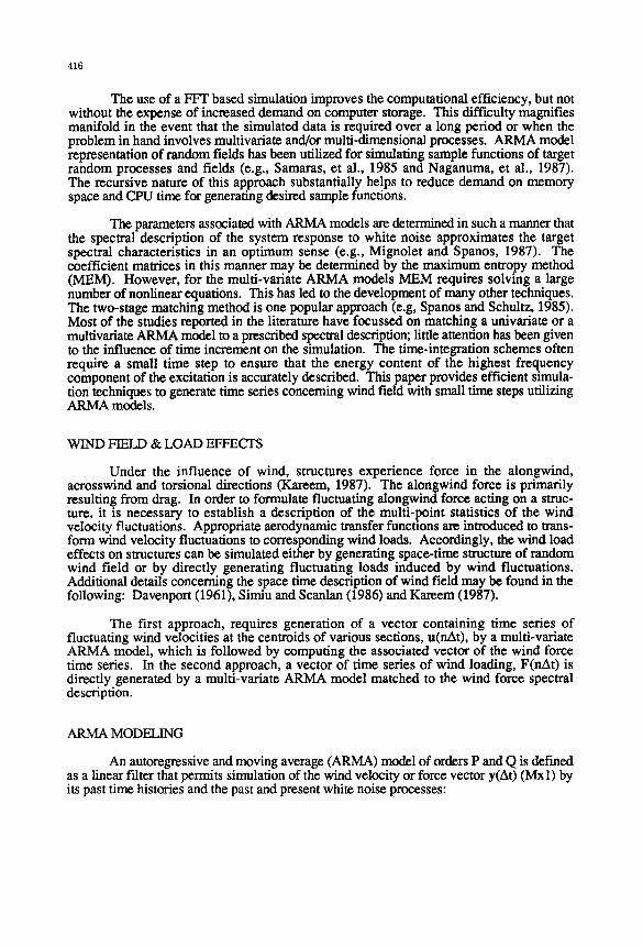
The use of a FFT based simulation improves the computational efficiency, but not without the expense of increased demand on computer storage. This difficulty magnifies manifold in the event that the simulated data is required over a long period or when the problem in hand involves multivariate and/or multi-dimensional processes. ARMA model representation of random fields has been utilized for simulating sample functions of target random processes and fields (e.g., Samaras, et al., 1985 and Naganuma, et al., 1987). The recursive nature of this approach substantially helps to reduce demand on memory space and CPU time for generating desired sample functions.

The parameters associated with ARMA models are determined in such a manner that the spectral description of the system response to white noise approximates the target spectral characteristics in an optimum sense (e.g., Mignolet and Spanos, 1987). The coefficient matrices in this manner may be determined by the maximum entropy method (MEM). However, for the multi-variate ARMA models MEM requires solving a large number of nonlinear equations. This has led to the development of many other techniques. The two-stage matching method is one popular approach (e.g, Spanos and Schultz, 1985). Most of the studies reported in the literature have focussed on matching a univariate or a multivariate ARMA model to a prescribed spectral description; little attention has been given to the influence of time increment on the simulation. The time-integration schemes often require a small time step to ensure that the energy content of the highest frequency component of the excitation is accurately described. This paper provides efficient simula- tion techniques to generate time series concerning wind field with small time steps utilizing ARMA models.

WIND FIELD & LOAD EFFECTS

Under the influence of wind, structures experience force in the alongwind, acrosswind and torsional directions (Kareem, 1987). The alongwind force is primarily resulting from drag. In order to formulate fluctuating alongwind force acting on a struc- ture, it is necessary to establish a description of the multi-point statistics of the wind velocity fluctuations. Appropriate aerodynamic transfer functions are introduced to trans- form wind velocity fluctuations to corresponding wind loads. Accordingly, the wind load effects on structures can be simulated either by generating space-time structure of random wind field or by directly generating fluctuating loads induced by wind fluctuations. Additional details concerning the space time description of wind field may be found in the following: Davenport (1961), Simiu and Scanlan (1986) and Kare~m (1987).

The first approach, requires generation of a vector containing time series of fluctuating wind velocities at the centroids of various sections, u(nAt), by a multi-variate ARMA model, which is followed by computing the associated vector of the wind force time series. In the second approach, a vector of time series of wind loading, F(nAt) is directly generated by a multi-variate ARMA model matched to the wind force spectral description.

ARMA MODELING

An autoregressive and moving average (ARMA) model of orders P and Q is def'med as a linear fiher that permits simulation of the wind velocity or force vector y(At) (Mxl) by its past time histories and the past and present white noise processes:

417

P

y(nAt) + Z Ary[(n-r)At] = Br en-r, r= I r=0

(1)

in which A r and B r ale AR and MA coefficient matrices, and en_ r is a vector containing white noise with a zero mean and a unit variance. The coefficient matrices are determined from the specified spectral description of the random field to be simulated. A desirable feature of ARMA modeling is that the model orders and the error are small, since the total order translates into the number of multiplications and additions at each discrete time interval during the simulation procedure.

ARMA models are characterized by poles and zeroes. A low-order ARMA model could produce a small error if the coefficients are suitably selected. The application of the maximum entropy condition to a multivariate ARMA model requires the solution of a large number of nonlinear equations. Therefore, some techniques have been developed to cir- cumvent this difficulty. One of these approaches is the two-stage-matching method, by which an ARMA model is developed based on a prior AR model. There are a number of different approaches that follow the two-stage-matching method e.g., (Samaras et al., 1984 and Spanos and Shultz, 1985). In this manner, an ARMA model can be formulated by the solution of a number of linear equations. This procedure is computationally convenient. However, ARMA model coefficients with given P and Q are not unique, since they depend on the prior AR order P'.

Altogether, there are three parameters to be selected: P', P, Q and At. Samaras et al. (1984) gave an empirical relationship,

P - - Q and P ' > P + Q + 2 . (2)

Optimal model orders may only be obtained from a larger number of combinations of the above parameters. In the present study, an interactive computer algorithm is developed to study the effects of various combinations of the parameters on the model accuracy. An empirical relation based on this study suggests

P' -- 3 (P + Q). (3)

Then for a fixed P+Q, a selection of P and Q can affect the model error. For the wind

field, it is recommended to use

P > Q. (4)

The time increment, At, also influences the model error. Approximately, the ARMA model involves a window of time period (P+Q) At. A decrease in At could increase the model error. The shape of the wind spectral density function can affect significantly the model accuracy. For example, an ARMA model used to match the wind spectrum with a finite value at the zero frequency, such as the Harris spectrum, has higher accuracy than an ARMA model for the wind spectrum with a zero value at the zero frequency, such as the Davenport spectrum. It is important to note that the ARMA matching is also sensitive to the accuracy of the correlation functions derived from a given spectral density function.

418

Typical examples of the comparisons between the target spectra and the estimated spectra are shown in Fig. 1, and the comparisons of the coherence functions are shown in Fig. 2. It is noted that an ARMA model can be matched to the Harris wind spectrum with almost no error in the entire frequency range. The main difficulty in matching the Davenport wind spectrum is due to the representation of the sharp drop in the spectral ordinates near the zero frequency.

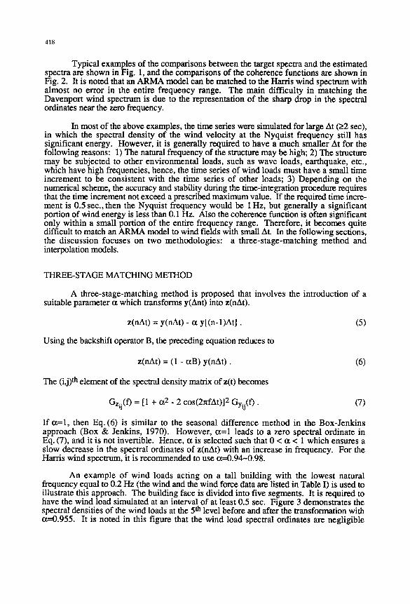
In most of the above examples, the time series were simulated for large At (>2 sec), in which the spectral density of the wind velocity at the Nyquist frequency still has significant energy. However, it is generally required to have a much smaller At for the following reasons: 1) The natural frequency of the structure may be high; 2) The structure may be subjected to other environmental loads, such as wave loads, earthquake, etc., which have high frequencies, hence, the time series of wind loads must have a small time increment to be consistent with the time series of other loads; 3) Depending on the numerical scheme, the accuracy and stability during the time-integration procedure requires that the time increment not exceed a prescribed maximum value. If the required time incre- ment is 0.5 sec., then the Nyquist frequency would be 1 Hz, but generally a significant portion of wind energy is less than 0.1 Hz. Also the coherence function is often significant only within a small portion of the entire frequency range. Therefore, it becomes quite difficult to match an ARMA model to wind fields with small At. In the following sections, the discussion focuses on two methodologies: a three-stage-matching method and interpolation models.

THREE-STAGE MATCHING METHOD

A three-stage-matching method is proposed that involves the introduction of a suitable parameter cc which transforms y(Ant) into z(nAt).

z(nAt) = y(nAt) - ct y[(n-1)At]. (5)

Using the backshift operator B, the preceding equation reduces to

z(nAt) = (1 - c~B) y(nAt). (6)

The (i,j) th element of the spectral density matrix of z(t) becomes

Gzij(f) = [1 + o~ 2 - 2 cos(2~fAt)] 2 Gyij(f). (7)

If c~=1, then Eq. (6) is similar to the seasonal difference method in the Box-Jenkins approach (Box & Jenkins, 1970). However, {z=l leads to a zero spectral ordinate in Eq. (7), and it is not invertible. Hence, ~ is selected such that 0 < ~ < 1 which ensures a slow decrease in the spectral ordinates of z(nAt) with an increase in frequency. For the Harris wind spectrum, it is recommended to use c¢=0.94~.98.

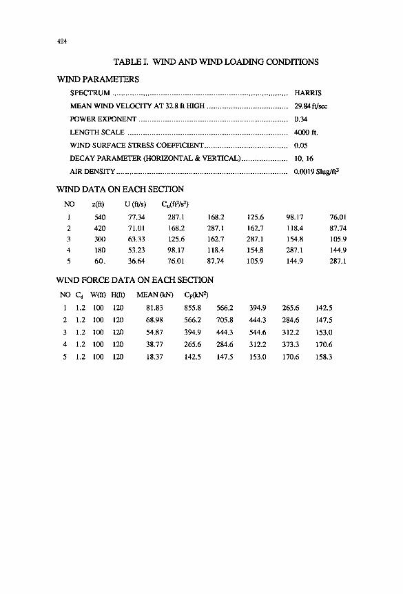
An example of wind loads acting on a tall building with the lowest natural frequency equal to 0.2 Hz (the wind and the wind force data are listed in Table I) is used to illustrate this approach. The building face is divided into five segments. It is required to have the wind load simulated at an interval of at least 0.5 sec. Figure 3 demonstrates the spectral densities of the wind loads at the 5 th level before and after the transformation with a,---0.955. It is noted in this figure that the wind load spectral ordinates are negligible

419

within the frequency range 0.1-1Hz. However, after the transformation, the spectrum covers the entire frequency range up to the Nyquist frequency and decays slowly with the frequency.

z(nAt) can be matched by an ARMA model utilizing the two-stage-matching procedure discussed in the preceding section,

5"PZ z(nAt) + ~ A~z[(n-r)At] = B r ~,n-r , (8)

r = l r=0

which, after substitution in Eq. (6), takes the form of Eq. (1), in which

and

P = P Z + I ,

I a 0 . . . 0

0 a . . . O A 1 -- A 1 - • : . . . 0

0 . . . . . . . . .

(9)

A r = A Z - ( ~ A z f o r t > 1 r -1

(10)

In this example, an ARMA (4,4) model from a prior AR (30) model has been matched for z(nAt). Subsequently, ARMA model (5,4) for y(nAt) is formulated. The spectral density of the target wind load and those represented by the ARMA model are plotted in Fig. 4. The results demonstrate the closeness between the target and estimated spectral functions.

The ARMA model representation given by the three-stage-matching method is especially suitable for describing the high frequency spectra. If the low frequency wind loads are not important, it is possible to obtain a very low order ARMA model, e.g., ARMA (3,1) for the above example. The three-stage-matching method involves a selection of the parameter a, in addition to P', P and Q. However, it does improve the shape of the spectral density functions, which facilitates a convenient modeling, but it cannot improve the shape of the coherence functions. Hence, the error in the correlation functions may not be small. Additional details may be found in Li and Kareem (1990). This method can be applied to most of the wind spectra, such as the Harris or Kareem spectra (Kareem, 1987). For some wind spectra, such as the Davenport spectrum, which has a zero ordinate at the zero frequency, this method is not suitable.

INTERPOLATION MODELS

A more general procedure to simulate time series of wind field involves a combination of an ARMA model and the interpolation model. Let the time increment in the ARMA model be At, such that the corresponding Nyquist frequency is a little larger than the frequency beyond which the wind has insignificant energy. Suppose that the time- integration scheme for the solution of the dynamic system requires a much smaller time increment St, where At /8 t is an integer S. It is required to formulate time series y[(nS+l~)St] from y(nAt) in which 1~ < S. There are a number of interpolation methods

420

available in the literature (e.g., Oppenheim & Schafer, 1989). Recently, new interpolation techniques with applications in engineering mechanics have been developed (Li, 1988). Their details will be reported elsewhere. Here some concepts relevant to wind engineering are introduced. First, it is important that the interpolation following an ARMA model satisfy the following requirements:

Local interpolation: y[(nS+~)&] is simulated from y(mAt) with m= n-Q1-, n-Qi-+l ..... n, .... n+Qi +, in which QI- and QI + are small integer numbers. The conventional global interpolation involving the total time series is not suitable for the present application.

Stability: The interpolation is said to be stable if a bounded time series after interpolation still remains bounded.

Accuracy: The spectral density functions represented by y[(nS+13)St] are the same as those of y(nAt) when the frequency is less than 1/2At, and zeros in the frequency range 1/2At- 1/28t.

The interpolation techniques may be classified as linear, polynomial and trigonometric. Frequently, a piecewise linear interpolation of the discrete data is utilized. This method is the simplest, but it may introduce a large error in the spectral density func- tion. The polynomial interpolation is the next level of interpolation. For example, Li (1988) developed a cubic polynomial interpolation, which results in a process continuous at its first-order time derivative, involving three multiplications and additions at each discrete time interval. The trigonometric interpolation suggested by Saunders and Collings (1980), is further developed in this study, and it is perceived to be the most suitable choice for wind engineering applications. In the following a basic concept of the trigonometric interpolation developed herein is presented:

pulses: The discrete time series can be viewed as a process, yat(t), consisting of numerous

yAt(t) = ~ y(nAt) At 8(t - nAt), (11)

in which 8(t-nAt) is the Dirac delta function. Its Fourier transform is written as

yAt(f) = ~ y(nAt) exp(-j2~f nat) At, n = - ~

(12)

which is a discrete Fourier transformation. The preceding equation shows that yAt(f) is cyclic with a cycle 1/At, and yat(f) =yat(1/A t _ ~ in which the overbar is the conjugate si~gn. Similarly, the time series with a time increment 8t can be viewed as a pulse process y~t(t), and the corresponding Fourier transformation becomes

ySt(f) = Z y(m8t) exp(-j 2~f mSt) St. (13)

Define a transfer function H(f) which satisfies

421

H(f) = ySt(f) (14) yat(0 "

For the ideal case, H(f)=l for f < I/2At and H(f)=0 for 1/28t < f < I/2At. Additional details are available in Li and Kareern (1990). The f'mal expression for ySt(t) is given by

y&[m&] = r=-SQ I+~1 h (r &) yat[(m-r)SX] , (15)

in which QI is the interpolation order, and h(rAt) the convolution kernel for interpolation is given by

m r h(r&) : H(rnAf) exp ( j g ) / ( 2 S Q ' ) , (16)

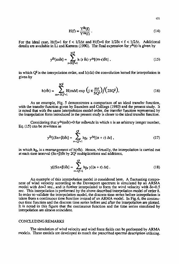
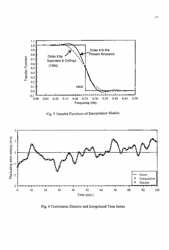
As an example, Fig. 5 demonstrates a comparison of an ideal transfer function, with the transfer function given by Saunders and Collings (1980) and the present study. It is noted that with the same interpolation model order, the transfer function represented by the interpolation form introduced in the present study is closer to the ideal transfer function.

Considering that yat(m&)--0 for m&-,~At in which n is an arbitrary integer number, Eq. (15) can be rewritten as

¢ - d

YSt[(Sn+l])&] = r=-~+~l hl~r Yat[(n + r) At], (17)

in which hi3 r is a rearrangement of h(r&). Hence, virtually, the interpolation is carried out at each tim'e interval (Sn+l])& by 2Q I multiplications and additions,

y[(Sn+13)&] = £ hl]r y[(n + r) At]. (18) ~-QI+I

An example of this interpolation model is considered here. A fluctuating compo- nent of wind velocity according to the Davenport spectrum is simulated by an ARMA model with At=2 see., and is further interpolated to form the wind velocity with 5t=0.5 sec. This interpolation is performed by the above described interpolation model of order 8. In order to validate the interpolation model, the discrete time series before interpolation is taken from a continuous time function instead of an ARMA model. In Fig. 6, the continu- ous time function and the discrete time series before and after the interpolation are plotted. It is noted in this figure that the continuous function and the time series simulated by interpolation are almost coincident.

CONCLUDING REMARKS

The simulation of wind velocity and wind force fields can be performed by ARMA models. These models are developed to match the prescribed spectral description utilizing,

422

among others, the two-stage-matching procedures. However, the nature of the dynamic systems and the numerical schemes utilized for the solution of the dynamic response often require a small time increment, which renders a straightforward application of ARMA models difficult. A three-stage-matching method is developed, in which a multivariate ARMA model of small time increments can be matched to a target wind spectrum. A salient feature of this method is that despite the low order of the model the spectral density function of the simulated data is in good agreement with the target spectral density function.

A more general technique utilizing an interpolation approach is presented. First, the time series is generated from an ARMA model with the time increment selected according to the maximum frequency of interest. Then by the interpolation technique the generated time series with large time increment is transformed into a time series with a smaller time increment. In this research a digital filter based on trigonometric interpolation is developed utilizing discrete convolution of finite and infinite waveforms. The two-stage proposed approach based on an ARMA model combined with an interpolation scheme offers a computationally efficient simulation procedure.

ACKNOWLEDGEMENT

The support for this research was provided in part by the PYI award to the second author by the National Science Foundation under Grant No. CES 8352223 and matching funds provided by a group of industrial sponsors.

REFERENCES

Box, G.E.P. and Jenkins, G.M. (1970), Time Series Analysis: Forecasting and Control, Holden-Day, San Francisco.

Davenport, A.G. (1961), "The Spectrum of Horizontal Gustiness Near the Ground in High Winds", Q. J. Roy. Met. Soc., Vol.87, pp.194-211.

Harris, R.I.(1968), "On the Spectrum and Auto-Correlation Function of Gustiness in High Winds", ERA Report 5273.

Kareem, A. and Dalton, C. (1982), "Dynamic Effects of Wind on Tension Leg Platforms," OTC 4229, Proceedings of Offshore Technology Conference, Houston, TX.

Kareem, A. (1985), "Wind-induced Response Analysis of Tension Leg Platforms," Journal of Structural Engineering, ASCE, Vol.111, pp.37-55.

Kareem, A. (1987), "Wind Effects on Structures: A Probabilistic Viewpoint," Probabilistic Engineering Mechanics, Vol. 2, No. 4, pp. 166-194.

Li, Y. (1988), "Stochastic Response of a Tension Leg Platform to Wind and Wave Fields," Ph.D. Thesis, Department of Mechanical Engineering, University of Houston.

Li, Y. and Kareem, A., "ARMA Systems in Wind Engineering," Probabilistic Engineering Mechanics, to appear in 1990.

Mignolet, M. P. and Spanos, P. D. (1987), "Recursive Simulation of Stationary Multivariate Random Processes - Part I," Journal of Applied Mechanics, ASME, Vol. 109, pp. 674-680.

Naganuma, T.,Deodatis, G., and Shinozuka, M. (1987), "ARMA Model for Two- Dimensional Processes," Journal of Engineering Mechanics, ASCE, Vol. 113 (2), pp. 234-251.

Oppenheim, A.V. and Schafer, R.W. (1989), Discrete-Time Signal Processing, Prentice-Hall.

Reed, D. A. and Scanlan, R. H. (1983), "Time Series Analysis of Cooling Tower Wind Loading," Journal of Structural Engineering, ASCE, Vol. 109, No. 2, pp. 538- 554.

423

Samaras, E., Shinozuka, M. and Tsurui, A. (1985), "ARMA Representation of Random Processes", Journal of Engineering Mechanics, ASCE, Vol.111, pp.449=461.

Saunders, L. R. and Collings, G. (1980), "Efficient Solution of Model Equations With Arbitrary Loadings", Eng. Struct., Vol.2, pp.35-48.

Shinozuka, M. (1971), "Simulation of Multivariate and Multidimensional Random Processes," Journal of the Acoustical Society of America, Vol. 49, pp. 357-367.

Shinozuka, M. and Jan, C.-M. (1972), "Digital Simulation of Random Processes and Its Application," Journal of Sound and Vibration, Vol. 25(1), pp. 111-128.

Simiu, E. and Scanlan, R. H. (1986), "Wind Effects on Structures," Second Edition, John Wiley & Sons, New York, NY.

Spanos, P.D. and Mignolet, M.P. (1987), "Recursive Simulation of Stationary Multi- variate Random Processes - Part II," Journal of Applied Mechanics, Vol. 54, pp. 681-686.

Spanos, P.D. and Mignolet, M.P. (1989), "MA to ARMA Modeling of Wind," Proceedings of the 6th U.S. National Conference on Wind Engineering (A. Kareem, editor).

Wittig, L. E. and Sinha, A. K. (1975), "Simulation of Multicorrelated Random Processes Using FFT Algorithm," Journal of Acoustic Society of America, Vol. 58, pp. 630-633.

424

T A B L E I. W I N D A N D W I N D L O A D I N G C O N D I T I O N S

W I N D P A R A M E T E R S

SPECTRUM ... . . . . . . . . . . . . . . . . . . . . . . . . . . . . . . . . . . . . . . . . . . . . . . . . . . . . . . . . . . . . . . . . . . . . . . . . . . . . . HARRIS

MEAN WIND VELOCITY AT 32.8 ft HIGH ... . . . . . . . . . . . . . . . . . . . . . . . . . . . . . . . . . . 29.g4 ft/sec

POWER EXPONENT ... . . . . . . . . . . . . . . . . . . . . . . . . . . . . . . . . . . . . . . . . . . . . . . . . . . . . . . . . . . . . . . . . . 0.34

LENGTH SCALE ... . . . . . . . . . . . . . . . . . . . . . . . . . . . . . . . . . . . . . . . . . . . . . . . . . . . . . . . . . . . . . . . . . . . . . . 4000 ft.

WIND SURFACE STRESS COEFFICIENT ... . . . . . . . . . . . . . . . . . . . . . . . . . . . . . . . . . . . 0.05

DECAY PARAMETER (HORIZONTAL & VERTICAL) .... . . . . . . . . . . . . . . . . . 10, 16

AIR DENSITY ... . . . . . . . . . . . . . . . . . . . . . . . . . . . . . . . . . . . . . . . . . . . . . . . . . . . . . . . . . . . . . . . . . . . . . . . . . . . 0.0019 Slug/ft 3

W I N D D A T A O N E A C H S E C T I O N

NO z(ft) U (ft/s) Cu(ftz/s a)

1 540 77.34 287.1 168.2 125.6 98.17 76.01

2 420 71.01 168.2 287.1 162.7 118.4 87.74

3 300 63.33 125.6 162.7 287.1 154.8 105.9

4 180 53.23 98.17 118.4 154.8 287.1 144.9

5 60. 36.64 76.01 87.74 105.9 144.9 287.1

W I N D F O R C E D A T A O N E A C H S E C T I O N

NO Ca W(ft) H(ft) MEAN(kN) C~(kN 2)

I 1.2 100 120 81.83 855.8 566.2 394.9 265.6 142.5

2 1.2 100 120 68.98 566.2 705.8 444.3 284.6 147.5

3 1.2 100 120 54.87 394.9 444.3 544.6 312.2 153.0

4 1.2 100 120 38.77 265.6 284.6 312.2 373.3 170.6

5 1.2 100 120 18.37 142.5 147.5 153.0 170.6 158.3

425

12000

90OO

E 600O , m

~ 3000

0 0.00

~ Target arris . . . . . . . Estimated by ARMA

ARMA for Harris: P'--30, P--Q=5, e=0.53% ARMA for Davenport: P'--30, P=6, Q=4, e=2.6%

t = 3.5 sec

Davenport ~ , • I • • • I • • • I • • • I i i i l , , . l

0.02 0.04 0.06 0.08 0.10 0.12 Frequency (Hz)

0.14

Fig. 1 Comparison of Estimated and Target Spectral Density Functions

1 . 0 ,

0.9 i 0.8 i 0.7 0.6 i 0.5' 0.4' 0.3 " 0.2 0.1 0.0

0.00 • _ ¶ , . I . . . !

0.02 0.04 0.06 0.08 0.10 Frequency (Hz)

Target Estimated (Harris) e=3.8% Estimated (Davenport) e=9.1%

i , , ,

0.12 0.14

Fig. 2 Comparison of Estimated and Target Coherence Functions

4 2 6

Oe+lO f 5e+10 [

eqZ~ 4e+10 ~

E 2 3e+10

o) 2e+10 t - "

0 2

(.9 le+10

0¢+0

Transformation: ~ = 0.955

. . . . . . . . . . . . . . . . , . . . . . . . . I I ''- -,

-1.2e+8

"G 1.0e+8

("4

z 8.0e+7

E --.i

"5 6.0e+7 ¢/2 "o

4.0e+7 a~

2 2.0e+7 ~

I.--- 0.0e+0

0.0 0.1 0.2 0.3 0.4 0.5 0.6 0.7 0.8 0.9 1.0 Frequency (Hz)

Fig. 3 Target Spectra Before and After Pre-Transformation

6e+10~

5e+10

4e+10 "G

3e+10 d ~

E 2 2e+10

13t.

t.O le+10

Oe+O 0.00

I ~ Target • Estimated

by ARMA(5,4)

C _ ~ . - " . . . . . A . . . .

0.02 0.04 0.06 0.08 0.10 Frequency (Hz)

Fig. 4 Target and Estimated Wind Load Spectra on the 5th Floor

4 2 7

1.1 1.0 0.9 0.8

.=_o 0.7

0.6 "= o.5

0.4 t--

0.3 I---

0.2

• Order e in the . . . . . . . . . J " ~, ~ I r P r e s e n t Research Order 8 b y " "'~.~k- I Saunders& Collings \ \ I (1980) "~[

0.1 Ideal 0.0

i -0.1

0.00 0.05 0.10 0.15 0.20 0.25 0.30 0.35 0.40 0.45 0.50 Frequency (Hz)

Fig. 5 Transfer Functions of Interpolation Models

E 1 v

O O

~ 0 " O t---

~-2 Lt..

-3 . . . . I • • ' , i . . . . I . . . . I . , • ' i . . . . I . . . . I • , , , i

0 10 20 30 40 50 60 70 80

i T Given Interpolation Discrete

90 100

Time (sec.)

Fig. 6 Continuous, Discrete and Interpolated Time Series