NBER WORKING PAPER SERIES

ARE YOU SURE YOU'RE SAVING ENOUGH FOR RETIREMENT?

Jonathan Skinner

Working Paper 12981http://www.nber.org/papers/w12981

NATIONAL BUREAU OF ECONOMIC RESEARCH1050 Massachusetts Avenue

Cambridge, MA 02138March 2007

I am grateful to the National Institute on Aging Grant PO1-AG19783 for financial support. I thankwithout implicating seminar participants at Washington University St. Louis, the NBER Summer Institute,Victor Fuchs, Michael Hurd, Alan Gustman, Laurence Kotlikoff, David Laibson, Annamaria Lusardi,Susann Rohwedder, Karl Scholz, Douglas Staiger, Steven Venti, Stephen Utkus, Jonathan Zinman,and especially the editors of the Journal of Economic Perspectives for helpful comments and suggestions.I am indebted to Laurence Kotlikoff for a copy of ESPlanner, and to Weiping Zhou for excellent researchassistance. The views expressed herein are those of the author(s) and do not necessarily reflect theviews of the National Bureau of Economic Research.

© 2007 by Jonathan Skinner. All rights reserved. Short sections of text, not to exceed two paragraphs,may be quoted without explicit permission provided that full credit, including © notice, is given tothe source.

Are You Sure You're Saving Enough for Retirement?Jonathan SkinnerNBER Working Paper No. 12981March 2007JEL No. D13,I11,J11,J14

ABSTRACT

Many observers believe current aging baby boomers are woefully unprepared for retirement. Othersraise the prospect that Americans are saving too much for retirement. This paper attempts to reconcilethese contrasting views using a simple life cycle model and a more sophisticated retirement program,ESPlanner, with special reference to retirement prospects for economists. I find most households withpost-graduate degrees fall short of the wealth needed to smooth spending through retirement. Of course,there are ways to economize during retirement: stepping up household production (cooking at homerather than eating out), selling one's house, or maintaining the modest individual consumption levelsfrom when children still roamed the house. But ultimately, I argue these laudable strategies to reduceretirement expenses will be dwarfed by rapidly growing out-of-pocket medical expenses. The combinationof eroding retiree health benefits and the risk of catastrophic future out-of-pocket health spendingsuggests that even conventional retirement planning recommendations could be too low.

Jonathan SkinnerDepartment of Economics6106 Rockefeller HallDartmouth CollegeHanover, NH 03755and NBERjonathan.skinner@dartmouth.edu

Many view the soon-to-retire Baby Boomers as woefully unprepared for their golden years.

Bernheim (1992) suggested this cohort was saving just one-third of what they needed to retire

comfortably. Christine Weller of the Economic Policy Institute stated that “the average American

household has virtually no chance to reach an adequate retirement savings in the next 50 years”

(Dugas, 2002). One recent report declared 43 percent of American households “at risk” of

substantial declines in retirement income, even after factoring in financial and housing wealth

(Munnell, Webb, and Delorme, 2006)

Other economists have taken a more sanguine view of American levels of saving (for

example Engen, Gale, and Uccello, 1999). Baby Boomers may not be accumulating much, but at

least they’re saving more than their parents did (Sabelhaus and Manchester, 1995; Keister and

Deeb-Sossa, 2001). Households don’t need to save because of reduced expenses as children leave

the household ((Scholz, Seshadri, and Khitatrakun, 2006b), or because they can rely on programs

such as Medicaid and Supplemental Security Income once they retire (Pauly, 1990; Hubbard,

Skinner, and Zeldes, 1995; Scholz, Seshadri, and Khitatrakun, 2006a).

And many feel that Baby Boomers just don’t need to spend as much once they retire

because of their greater ability to cut back on expenses (Brock, 2004). Aguiar and Hurst (2005a, b)

find that retired households spend less money and engage in more “home production” such as

shopping for lower prices, even while maintaining the quality and quantity of caloric intake through

retirement. Finally, if Americans are failures at saving enough for retirement, why are some

retirees so happy? As one wrote to the New York Times (as quoted in Loewenstein, Prelec, and

Weber , 1999): “You can get by on a lot less when you’re retired, without really depriving yourself

of anything important…. If I had known earlier how much ‘wealth’ derives from such simple

2

pleasures, I would have retired a lot sooner.” Indeed, some financial planners have evolved into

“life planners” who encourage clients to reevaluate their life priorities rather than accept the status

quo of meaningless materialism (Eisenberg, 2006).

This paper attempts to reconcile these widely diverging views of saving adequacy. The

seemingly simple question of “Am I saving enough for retirement?” is apparently not so simple at

all. Instead, it touches on a variety of deeper issues in economics, psychology, and health policy.

As a starting point, several observations seem to hold true. First, wealth requirements necessary to

maintain steady consumption through retirement are indeed daunting for many households, even

those with generous 401(k) plans and high incomes. (Readers are warned that life-cycle retirement

wealth targets presented below may lead to feelings of financial inadequacy.) Most households

cannot save enough to guard against all future contingencies, such as dramatically lower rates of

return on investments or unexpected earnings losses near planned retirement.

Second, while smoothing consumption through retirement may not be the sine qua non of

retirement planning, it’s not entirely clear what is needed for retirement security. In theory,

prospective retirees know they can always move to smaller houses or to less expensive regions of

the country, or cook at home rather than eating out, but how will their future selves feel about

calling the moving van or seeking out less expensive stores? There is no simple answer to this

question, because retirement is such a heterogeneous experience that depends on health and

temperament as well as wealth (Kelly, 1958). Still, one can conclude that many newly retired

households both anticipate a modest decline in consumption, and adjust to it.

The final observation is that retirement encompasses both age 66, when healthy households

can easily substitute leisure for market expenditures on food, and age 86, when few can substitute

home production for purchased health care. Growth rates for out-of-pocket health care spending

3

have kept pace with overall health care cost growth, and thus continue to outstrip GDP growth, or

may accelerate as firms jettison retiree health benefits. These health care cost projections are

perhaps the scariest beast under the bed. Fronstin (2006) estimates that a 55-year-old couple in

2006, planning to retire at age 65, would need to accumulate more than $400,000 during the next

10 years in order to afford supplemental health costs, beyond what Medicare already covers,

through age 90. Even in the near term, projections based on the Health and Retirement Study

suggest that by 2019, nearly one-tenth of elderly retirees will be devoting more than half of their

total income to out-of-pocket health expenses. Thus, saving for retirement may ultimately be less

about the golf condo at Hilton Head and more about being able to afford wheelchair lifts, private

nurses, and a high-quality nursing home.

Retirement Saving in a Life Cycle Model

A good starting point for calculating retirement saving is the standard life cycle model in

which consumption (adjusted for family size) is flat over the life cycle and so is “smoothed”

through retirement. Thus, households save while working in order to finance income shortfalls

during retirement. Of course, depending on levels of risk, and on how the rate at which individuals

discount future consumption compares to the after-tax interest rate, a flat path of consumption may

not be optimal, but it is a reasonable first start, and is consistent with observed growth rates in

consumption near retirement (Bernheim, Skinner, and Weinberg, 2001).

How Much Wealth Do You Need to Smooth Consumption Through Retirement?

The first task of this paper is to calculate how much wealth you should own to smooth

consumption. These calculations are performed only for those aged 40 and up. Readers in their

20s and 30s should be maximizing their workplace matching contributions (Benartzi and Thaler,

4

forthcoming), seeking automatic saving mechanisms such as house mortgages, and hoping that their

generation can still look forward to solvent Social Security and Medicare programs.

I will focus here on non-housing net worth, under the working assumption that most

households value the option of remaining in one’s house until declining health forces a move or a

sale (Lusardi and Mitchell, 2006). Count up 401(k) plan balances, IRAs, business equity, stock

investments, equity in second houses, and so forth, but do not count defined benefit pension plans

that pay a fixed amount at retirement, or prospective Social Security payments; these will both be

included as components in retirement income flows. Take the ratio of net non-housing wealth to

before-tax income.

The next step is to calculate the hypothetical target wealth that would allow for smoothing

consumption through retirement. Note that the intertemporal budget constraint specifies that (a)

current non-housing net wealth plus (b) the present value of net earnings, pension flows, and Social

Security benefits is equal to (c) the present value of non-housing consumption plus bequests.

Ignoring bequests for the moment, the unknown wealth level (a) – that is, the difference between

(c) and (b) -- is the level of current wealth that would ensure a consumption path sustainable

through retirement as long as the household shall exist. This target wealth is “The Number”; if

current assets are below the number, you’re not saving enough, or you need to plan for a reduction

in consumption at retirement.1 In a simplified life cycle, just a few parameters are necessary to

calculate this target wealth: 1) current age, expected retirement age, marital status, and retirement

planning horizon; 2) the expected real rate of return or interest rate; 3) the mortgage payment rate as

a fraction of earnings, where the mortgage is assumed paid off by retirement; 4) the saving rate, as a

1 “The Number,” the subject of Eisenberg’s (2006) breezy book, is a bit different, because it is the amount of money one needs to retire today to pursue one’s life goals.

5

fraction of before-tax earnings; 5) the retirement “replacement rate” β, or the fraction of retirement

annuity flows divided by pre-retirement earnings.

Retirement annuity flows should include any income from a defined benefit pension plan,

but for many Baby Boomers (and most academics), the only guaranteed income transfers will

consist of Social Security benefits. These are anticipated to pay an annual maximum of $33,390 (in

2006 dollars) in 2031 for an age-65 individual with spousal benefits, or $45,240 if both members of

the family contribute to the 2006 maximum of $94,200. Amounts are more if retirement is

deferred, and could turn out to be less if Social Security is trimmed back under the weight of its

long-term obligations.2 I adopt a value of β = 0.3, which is consistent with final-year income of

$120,000 and Social Security payments of $40,000. Converting wealth to annuities would further

allow households to increase β at the expense of current wealth.

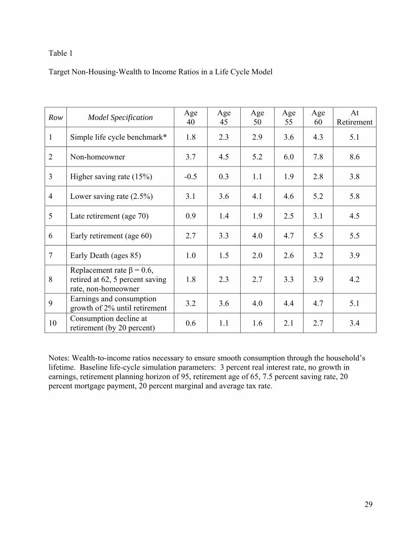
The first row of Table 1 displays asset-income ratios for a set of benchmark parameters: a

replacement ratio β of 30 percent, real interest rate of 3 percent, retirement age 65, planning horizon

of age 95, 20 percent average and marginal tax rate, mortgage payments comprising 20 percent of

income, and the flow of new savings equal to 7.5 percent of before-tax earnings. (Relatively few

Americans work until 65, but academics do tend to retire later than the general population.) At age

40, the non-housing wealth-to-income ratio is 1.8, rising to 2.9 at age 50 and peaking at 5.1 when

retirement occurs.

Sensitivity of “The Number”

The first sensitivity analysis, in Row 2 of Table 1, shows the importance of housing wealth in

attenuating the need to accumulate non-housing wealth for retirement. Renters would need to set

2 An alternative approach is to take current wealth as given, and calculate necessary replacement rates, with more elaborate models accounting for sources of investment, longevity, or health risk (VanDerhei, 2006).

6

aside 8.6 times income by the time they retire to afford both non-housing consumption (as above)

plus 30 years of future rental payments. Thus paying off the mortgage by retirement reduces non-

housing wealth requirements substantially.

Target wealth is also sensitive to changes in the saving rate; the wealth-income ratio at age

40 is -0.5 when the saving rate is 15 percent, and 3.1 when the saving rate is 2.5 percent (Rows 3

and 4). One puzzle is why wealth requirements at retirement are so much larger for the household

saving 2.5 percent (5.8 times income) instead of 15 percent (3.8 times income). After all, the

saving rate might not seem to matter once households reach retirement. The resolution of the

puzzle is to note that the high saving household has gotten used to a lower rate of consumption

while working, so less is needed to smooth consumption through retirement. Raising saving rates

therefore yields a “double dividend” in life-cycle saving by stimulating asset accumulation and

attenuating future required consumption.

Extending retirement age to 70 (Row 5), not uncommon among academics, sharply reduces

required wealth accumulation at all ages, while retiring early at 60 (Row 6) raises wealth

accumulation. As Row 7 demonstrates, dying early is another approach to ensuring retirement

security. A scenario closer to a lower income worker who doesn’t own a house -- a replacement

ratio of β = 0.6, a retirement age of 62, and a saving rate of 5 percent -- yields a wealth/income

target of 1.8 at age 40, rising to 4.2 at retirement (Row 8). Finally, allowing earnings to grow in

real terms at 2 percent, coupled with consumption growth of 2 percent until retirement, leads to

even larger wealth requirements relative to the benchmark, since consumption growth also raises

the level of retirement consumption (Row 9).

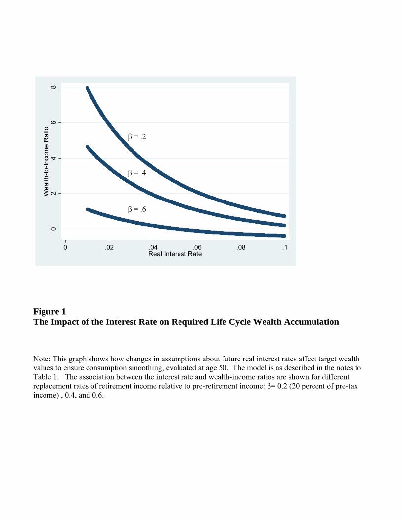
Figure 1 demonstrates the sensitivity of retirement savings to two important factors: the

income replacement ratio β and the interest rate. The target retirement wealth ratio is graphed for

7

different values of the replacement rate β (0.2, 0.4, and 0.6) and the interest rate. Note that the

wealth target is not particularly sensitive to the interest rate when β = 0.6. When the household

saves (7.5 percent of earnings), and pays a mortgage (20 percent of earnings) and income taxes,

what’s left over for consumption is sufficiently small to be taken care of by retirement income

flows. Thus high replacement rates help to insure against the risk of interest rate fluctuations. By

contrast, when saving requirements are much greater, as in the case where β = .2, “The Number” is

highly sensitive to adverse outcomes in equity and bond markets. It ranges from below one (that is,

wealth less than current income) for a 10 percent rate of return, to 8.0 for a laggard 1 percent

return.3

This model ignores many factors potentially relevant to retirement planning, such as tax-

deferred accounts (where balances are typically pre-tax dollars before being distributed from the

account), the progressivity of the tax code, children’s expenses (including college or bail bonds),

mortgage payments, estate planning, and a variety of other factors. To handle this additional

complexity, I turn to ESPlanner, a commercial retirement planning program built on the same life-

cycle framework simulated in Table 1, but with all these other factors relevant for saving plans built

in.4 I use several representative income levels based on the 2005 annual American Economic

Association survey of economics departments, kindly supplied by John Siegfried (Vanderbilt) and

Charles Scott (Loyola, Maryland).

3 This model assumes a steady state with constant real interest rates. Were interest rates to fluctuate, the calculations would be affected by simultaneous changes in the market value of assets held by the household. 4 It was programmed originally by Jagdeesh Gohkale and Laurence Kotlikoff. Kotlikoff (2006) argues persuasively that this model provides better financial advice than popular alternatives. In the program, I determined target wealth iteratively to within a tolerance of under $50 between actual and recommended consumption.

8

The income distribution is based on median earnings at schools (not individuals), but the

percentiles are weighted by the number of faculty at each institution. I begin with what is a

relatively low baseline academic-year income for full professors, $68,000, at the 10th percentile

(from the bottom) of B.A.-granting colleges. This rises to $88,000 for the median and $126,000 at

the 95th percentile. By contrast, the 10th percentile salary for full professors at Ph.D.-granting

institutions is $104,000, the median $134,000, and the 95th percentile $184,000. To span these

ranges, I adopt multiples of $68,000, reaching as high as $272,000 to capture the hypothetical

income of very well-compensated dual working households (or a part-time finance professor).

These calculations cannot be generalized to the wealth requirements of low-income households

whose saving needs may be more modest owing to more generous replacement rates in Social

Security or from Social Security Disability Insurance (Bernheim et al., 2000, although see

VanDerhei, 2006).

Table 2 provides these target wealth holdings by age for single and married households for a

variety of income and demographic scenarios. The detailed inputs are described in the notes to

Table 2; the surprising feature is how important all of these additional variables are for retirement

planning. The house is assumed to be worth 2.5 times income, and the mortgage balance, with 20

years remaining, is initially equal to twice income. The equivalence scale of a spouse is assumed to

augment consumption by 0.6, while each child increases the consumption requirements of the

household by .25.5 I assume a baseline saving rate equal to 7.5 percent of pre-tax income, with 5

percent to a 401(k) and 2.5 percent to non-retirement assets, split equally between bonds and

stocks. This is a flow measure, and underestimates the real saving rate which includes capital

5 The total equivalence scale for two adults and two children in this model, 2.1, matches the OECD-modified equivalence scale (although they place slightly more weight on children and less on adults); for a very succinct introduction see OECD (2005).

9

gains, the reinvestment of interest and dividend income, and any appreciation in housing equity.

An important assumption implicit in this model is that once the house mortgage is paid off, monthly

payments are diverted to saving, not consumption.

Consider the simplest case, of a single person with income of $68,000, and whose

contingency planning allows for a 95-year lifespan. As in the previous analysis, I focus solely on

non-housing wealth. The first row in Table 2 shows that wealth at age 40 necessary to sustain a

constant consumption flow is just $14,000. By retirement, non-housing wealth has grown to

$272,000, somewhat below the prescribed wealth-to-income ratio in Table 1. For households with

children (Row 2), target wealth levels in a household with $68,000 in income are higher during

their 40s in anticipation of college expenses. For single households earning $136,000 annually

(Row 3), wealth requirements are substantially greater, $964,000 at retirement, because the

progressivity of Social Security payments leads to a lower replacement rate β. Home ownership

reduces target wealth (Row 4 versus Row 3) because the homeowner need not save against future

rental payments during retirement (as in the example above), and because of the extra saving gained

by paying off the mortgage at age 60.

For married households with two children and income of $136,000, saving requirements are

$167,000 at age 40, rising to $850,000 prior to retirement (Row 5). In the presence of a defined

benefit plan that pays 30 percent of before-tax income, however, wealth requirements drop

substantially, with prescribed wealth of only $95,000 at age 65 (Row 6). This is because combined

Social Security and pension payments match the consumption of the empty-nest couple (and the

surviving spouse) quite closely. As one moves up the income distribution (Rows 7 – 10), target

wealth measures rise accordingly, but the wealth-to-income ratio for these higher income groups is

actually a bit lower; for example, the wealth-to-income at retirement for the household earning

10

$136,000 (Row 5) is 6.2, but is only 5.6 for the household earning $272,000 (Row 10). This pattern

largely reflects the progressivity in the tax code leading to less-than-proportional increases in

lifetime consumption streams.

A comparison of Rows 8 and 9 suggests a somewhat smaller interest elasticity of target

wealth than that suggested by the earlier simulations, in part because the discount rate is less

important for college expenses, and also because of declining total expenditures as first children,

and then a spouse, leaves the household. Table 2 also demonstrate that the presence of children,

with equivalent scale measures of 0.7, actually reduces required wealth accumulation (Row 11

compared to Row 3), and that wealth requirements necessary to plan for a future in which the

spouse spends five years in a nursing home, are indeed daunting (Row 12 compared to Row 8).

These topics are taken up in more detail below.

How Much Money Do You Really Need to Enjoy Retirement?

As noted above, a variety of studies show that most American households fail to meet

saving goals suggested by certainty life-cycle models (Ameriks and Utkus, 2006; Warshawsky and

Ameriks, 2000; Shackleton, 2003; Munnell, Webb, and Delorme, 2006; Mitchell and Moore, 1998;

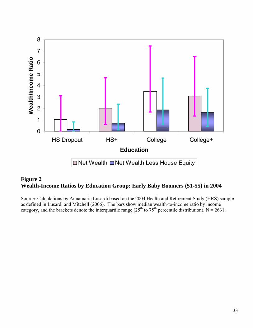
Lusardi and Mitchell, 2006). Figure 2 shows that even Baby-Boomers aged 51-55 with post-

graduate degrees fall short of the conventional savings targets calculated above; the median non-

housing wealth-to-income ratio is 1.7, with the 25th percentile just 0.5 (Lusardi and Mitchell, 2006).

Many well-educated Baby Boomers will likely need to scale back consumption at retirement. But

does this mean that they’ve failed to save “enough”? Here I consider several explanations for why

consuming less at retirement might not imperil retirement security.

11

Housing Equity Can Be Used to Finance Consumption During Retirement

Some financial planners have noted how much retirees could save simply by unleashing

their housing equity and moving to towns such as Henderson, Nevada, where living cost are less

than half that in New York (Brock, 2004, p. 74).6 A more limited approach would be to purchase a

smaller house or condominium in the same town. If one is planning to downsize in the future, it’s

okay to add some part of housing equity to the retirement nest-egg available for non-housing

consumption – but the value should be discounted, perhaps at a risky rate of return. In practice,

Venti and Wise (1989) have shown that recent retirees are about as likely to move into more

expensive as less expensive housing. The exception occurs when there are adverse transitions such

as widowhood or serious illness, at which point households are more likely to tap into housing

equity (Venti and Wise, 2004). Thus, average housing equity tends to decline with age, particularly

among older households (Hurd, 2003).

Still, future retirees are typically unwilling to commit having to move to a smaller house.

Lusardi and Mitchell (2006) found nearly 70 percent of respondents to the Health and Retirement

Survey aged 70 and under felt there was a minimal (10 percent or less) chance of selling their house

to pay for retirement (see also Smeeding et. al., 2006). Reverse mortgages allow retirees to borrow

money against housing equity, to be repaid upon death, but in practice their use has not been

widespread (Sun, Triest, and Webb, 2006).

A middle ground recognizes the option value of housing equity for future uncertain

contingencies. Housing equity is perhaps the best hedge against future catastrophic health care

costs, because such equity is often exempted from Medicaid asset limits, and because patients with

expensive chronic illnesses who require specialized health care would need to vacate their house in

6 Of course, this strategy begs the question of why housing costs are so low in Henderson, Nevada.

12

any case (Skinner, 2004). Even if these adverse events don’t occur, home equity can still provide a

bequest to children or other worthy causes (Dynan, Skinner, Zeldes, 2002).

With Children Gone (Or A Spouse Lost), Consumption Expenses Are Lower During Retirement

Any parent will bemoan the expenses of raising children, ranging from diapers early in the

life cycle to college education and helping out with housing down-payments later. For this reason,

parents may reasonably expect a decline in family consumption as the children depart. The

importance of children in life-cycle consumption and saving was emphasized by Scholz, Seshadri,

and Khitatrakun (2006a,b), who found 80 percent of U.S. households were optimally saving for

retirement after accounting for the timing and influence of children on optimal consumption plans.

Equivalence scales were used to adjust household consumption for differences in the size and

composition of it members. Their equivalence scale, from Citro and Michael (1995), implied that a

married couple with two children now consuming $40,000 can smooth person-equivalent

consumption by planning for $24,600 in expenditures once the children have left, and $17,000

following the departure of a spouse. 7

The importance of equivalence scales can also be seen in ESPlanner by comparing Row 11

in Table 2, a single parent with two children against Row 4, a single person without children. (In

Row 11, the ESPlanner default equivalence scale of 0.7 per child is used.) Target wealth at age 40

is $18,000 for the household with children, and $282,000 for the household without! Despite the

additional expense of college, retirement saving is diminished for the parent with children because

her annual consumption at retirement is just $49,301, rather than the $63,445 required for the single

household.

7 The classic study of how demographic factors affect life cycle consumption is Attanasio, Banks, Meghir, and Weber (1998), who find more modest effects of children and spouses on consumption.

13

In other words, parents are already used to getting by on peanut butter, given that a large

fraction of their pre-retirement budget has been devoted to supporting children, so it’s not difficult

to set aside enough money to keep them in peanut butter through retirement. By contrast, childless

households with the same income accustomed to caviar and fine wine must set aside more assets to

maintain themselves in the style to which they have become accustomed. This assumption is

central to why both the Scholz, Seshadri, and Khitatrakun studies, and Kotlikoff’s own studies

using ESPlanner, show that many households are saving too much for retirement (Darlin, 2007).

In practice, whether parents should plan to continue consuming just peanut butter is not entirely

clear, particularly if they want to substitute into more consumption for themselves, or if they value

strategic bequests and the warm glow from inter vivos transfers.

There Are Ample Opportunities to Economize While Retired

It is reasonable to believe that households need not spend as much during retirement, given

the sudden increase in leisure time.8 In this view, retirement is an opportunity to substitute leisure,

or home production, for market expenditures, given that the “price” of labor inputs into the

household production (or the reservation wage) has just fallen (Ghez and Becker, 1975). For

example, retirees now have more time to cook spaghetti sauce at home rather than buy prepackaged

sauce, or purchase lower cost but equally nutritious food. And it is certainly true that if households

can plan on a decline of (say) 20 percent at retirement, their target wealth while younger declines

substantially, from a wealth-income ratio of 2.3 to only 1.1 at age 45 (Table 1, Row 10).

8 It might appear that retiring from a job frees up expenditures on commuting, work-related

clothing, and other expenses associated with employment. However, work-related expenses do not appear to account for much of the consumption decline (Bernheim, Skinner, and Weinberg, 2001).

14

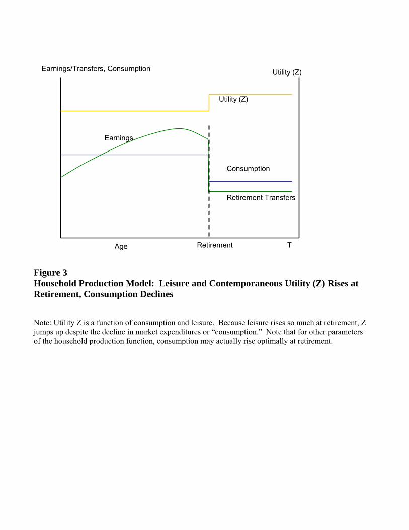
Consider an economic model in which leisure and consumption expenditures are combined

to create contemporaneous utility Z. For those who retire voluntarily, Z will rise simply because

the wage rate, or the price of a major input into the household production function, has declined.

This can be shown in Figure 2, where the contemporaneous utility Z jumps up discontinuously at

retirement. It is straightforward to show in a constant-elasticity-of-substitution utility function that

consumption smoothing is optimal only when the intertemporal elasticity of substitution of Z – or

the ease of substituting utility from one time period to the next -- is equal to the intratemporal

elasticity of substitution between consumption and leisure.9

Intuition might suggest that optimal consumption expenditures should drop discretely at

retirement, as is shown in Figure 3. However, this result holds only when the intertemporal

elasticity is less than the intratemporal elasticity – meaning that households can more easily

substitute leisure for consumption than shift household production (or Z) to later in life.

Conversely, when the intratemporal elasticity is less than the intertemporal elasticity, optimal

consumption is predicted to rise at consumption, meaning that households would save more so they

could really enjoy themselves during their retirement years.

There is mixed evidence on the relative magnitude of these elasticities; some imply a rise at

retirement (for example, Kniesner and Ziliak, 2005), while others imply a decline. Aguiar and

Hurst (2005a) find that recently retired households are remarkably efficient in home production,

saving large amounts of market expenditures while maintaining both the quality and quantity of

food. Similarly, Aguiar and Hurst (2005b) find that in a cross-section of shoppers in Denver, prices

9 The intratemporal elasticity is related closely to the labor supply elasticity. In standard

notation, lifetime utility U = (1-1/γ)-1 ∑t Zt1-1/γ

(1+δ)1-t and Zt = (Ct1-1/ρ+ ηLt

1-1/ρ)[1/(1-1/ρ)] with C and L denoting consumption and leisure, δ the time preference rate, ρ the intratemporal elasticity of substitution, γ the intertemporal elasticity of substitution, and η measuring the relative taste for leisure. Alternatively, smoothing holds when consumption and leisure are strongly separable.

15

for identical packaged goods varied systematically across demographic groups, with higher income

and middle-aged people paying more and younger and older households less.

Distinguishing between consumption and home production can potentially resolve a puzzle

in the data; 73 percent of retirees wished they had saved more (Hurd and Zissimopoulos, 2003), yet

the majority of voluntary retirees are as happy or happier being retired (Loewenstein et al., 1999;

Charles, 2002; Bender, 2004). These retirees may not have saved enough for the retirement they

thought they wanted, but the additional leisure cannot help but to raise their utility and create good

cheer. The story is different when retirement is involuntary because of job separation or poor

health, which occurs for 37 percent of the Health and Retirement Study (Bender, 2004). For this

group, subjective well-being declines (Charles, 2002), a decline that could also reflect a much

diminished household production function.

There is a remarkable heterogeneity in the saving adequacy of households, even in academic

settings (Bernheim, et. al., 2002). Perhaps 20 percent of households arrive at retirement with

generous replacement rates (β) and asset-to-income ratios, and these households do smooth

consumption, or even increase consumption by a small amount. These households also spend more

time cooking and shopping (Schwerdt, 2005). But for the one-third of the population with

inadequate replacement rates and wealth accumulation, consumption declines by one-third or more,

not because of any specific economic theory, but because of the unrelenting discipline of the budget

constraint (Bernheim, Skinner, and Weinberg, 2001). Households largely anticipate the decline

(Hurd and Rohwedder, 2006), with the exception of those who didn’t plan well for retirement,

where nearly one-quarter are surprised by how high their expenses are at retirement (Ameriks,

Caplin, and Leahy, forthcoming). What we don’t know is whether this heterogeneity in wealth

accumulation at retirement reflects natural variation in the household production function (some are

16

better at making spaghetti sauce than others) or heterogeneity in psychological biases towards

saving (Bernheim and Rangel, 2005).10

Evidence that favors psychological explanations for variations in wealth accumulation come

from the literature on 401(k) plan participation, in which simple changes in program participation

default rules, so that workers must opt out of a 401(k) rather than opt in, had a dramatic impact on

participation rates (Madrian and Shea, 2001; Choi, Laibson, Madrian, and Metrick, 2004). In this

issue, Benartzi and Thaler discuss this and other default rules involving issues such as the level of

contributions to a retirement savings account over time and how those savings are invested.

Similarly, Lusardi (1999) and Ameriks, Caplin, and Leahy (2003) suggest that simply planning for

retirement encourages greater savings, while Lusardi and Mitchell (2006) find financial literacy –

whether households understand compound interest – is also associated with higher levels of wealth.

From this perspective, the lack of wealth at retirement for many Americans may not be the

consequence of well-formed preferences, but instead of procrastination or inertia.

However, behavioral models cut both ways in terms of whether retirees will be happy with

the savings choices they made earlier in life, because these models also have demonstrated that

people have the ability to adapt to new circumstances. For example, paraplegics report happiness

levels that are not so far from lottery winners (Brickman, Coates, and Janoff-Bulman, 1978). By

comparison, learning to live with a 20 percent decline in consumption at age 66 shouldn’t be too

difficult, particularly for those in comfortable economic circumstances. If households are able to

replicate the same nutritional consumption flow post-retirement with relatively little effort, as in

10 Another possibility is variation in time-preference rates. However, Bernheim, Skinner, and Weinberg (2001) found no evidence that consumption growth rates differed across these groups prior to retirement, when households should be least likely to encounter liquidity constraints.

17

Aguiar and Hurst (2005a), it could even prompt households to wonder why they hadn’t economized

on expensive food expenditures years before.

Some retirement planners go one step further, taking on the role of life-cycle therapist, and

trying to understand what makes baby boomers happy. As Eisenberg (2006, p. 251) gently

admonishes, “you’re simply trapping yourself in a never ending cycle of acquisition and you

haven’t even taken a stab at figuring out what it would cost to do what you really want.” In other

words, why work until age 65 to maintain a $150,000 per year consumption habit where by retiring

early, one can live a fulfilling life on “only” $100,000 annually? Recognizing that money may not

buy happiness, Eisenberg suggests instead that retirement may be better spent in early-morning

meditation, spending a few hours writing “the great American novel,” and then volunteering at a

community center. But when the client becomes too sick or frail to write a novel and needs

volunteers to visit her – then what?

The Real Worry: Growing Out-of-Pocket Health Care Costs

Models of retirement planning with perfect certainty are likely to understate the risks from

poor health. First, there are risks to future income and wealth from poor health prior to retirement.

In a 10-year period, seven out of ten adults aged 51-61 developed health problems, lost their jobs,

or lost spouses owing to divorce or death (Johnson, Mermin, and Uccello, 2005; also see Smith,

2005). Most of these shocks had a sharp adverse impact on wealth: among couples, a new medical

condition caused a 17 percent decline in wealth for couples, work disability caused a 16 percent

decline and divorce a 44 percent decline, presumably the consequence of uninsured legal fees and

other contingencies (Johnson, Mermin, and Uccello, 2006). Typically, complex dynamic

programming models call for higher levels of precautionary saving to guard against such risks.

18

Once retired, health care is a commodity were opportunities for substitution between leisure

and market expenditures is limited. Poor health both restricts the ability of elderly people to engage

in home production (for example, if they can no longer drive around to search for low prices) while

increasing demand for expensive health care. Also, the elderly face substantial financial risk from

health care expenditures (McGarry and Shoeni, 2005; Goldman and Zissimopoulos, 2003; French

and Jones, 2004).

Currently, Medicare requires a 20 percent copayment and a one-day deductible for hospital

stays. Most retirees have a “Medigap” plan that covers these out-of-pocket liabilities, while

Medicaid picks up the difference for those with low-incomes who are eligible. But the percentage

of private-sector employers offering retiree health benefits has eroded, from 20 percent in 1997 to

just 13 percent in 2002 (Fronstin, 2005). Even academic institutions are shedding their retiree

health benefits; only 76 percent offered such benefits in 2004, and many of those are planning to

drop coverage within the next five years (Fronstin and Yakoboski, 2005). As noted earlier, a 55-

year-old couple retiring in 2016 will need to accumulate more than $400,000 over the next decade

to pay for Medigap insurance (Fronstin, 2006), and this sum does not include protection from

nursing home expenditure risk.

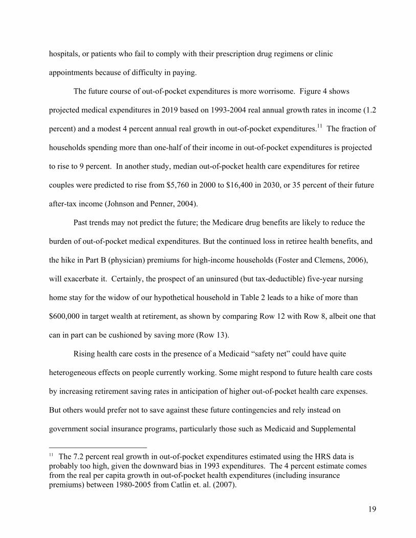
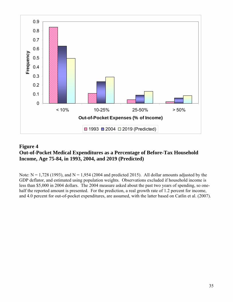
To capture the distribution and growth of these expenditures, estimates of out-of-pocket

medical expenditures for households age 75-84 were estimated from 1993 and 2004 in the Health

and Retirement Study (HRS); these are shown in Figure 4. Two percent of households experienced

out-of-pocket expenses in 1993 in excess of 50 percent of their before-tax income. (This probably

understates the true distribution because the initial sample comprised non-institutionalized

households.) By 2004, this fraction had risen to 6 percent, with an additional 9 percent paying

between 25-50 percent of income. These estimates do not reflect unpaid bills written off by

19

hospitals, or patients who fail to comply with their prescription drug regimens or clinic

appointments because of difficulty in paying.

The future course of out-of-pocket expenditures is more worrisome. Figure 4 shows

projected medical expenditures in 2019 based on 1993-2004 real annual growth rates in income (1.2

percent) and a modest 4 percent annual real growth in out-of-pocket expenditures.11 The fraction of

households spending more than one-half of their income in out-of-pocket expenditures is projected

to rise to 9 percent. In another study, median out-of-pocket health care expenditures for retiree

couples were predicted to rise from $5,760 in 2000 to $16,400 in 2030, or 35 percent of their future

after-tax income (Johnson and Penner, 2004).

Past trends may not predict the future; the Medicare drug benefits are likely to reduce the

burden of out-of-pocket medical expenditures. But the continued loss in retiree health benefits, and

the hike in Part B (physician) premiums for high-income households (Foster and Clemens, 2006),

will exacerbate it. Certainly, the prospect of an uninsured (but tax-deductible) five-year nursing

home stay for the widow of our hypothetical household in Table 2 leads to a hike of more than

$600,000 in target wealth at retirement, as shown by comparing Row 12 with Row 8, albeit one that

can in part can be cushioned by saving more (Row 13).

Rising health care costs in the presence of a Medicaid “safety net” could have quite

heterogeneous effects on people currently working. Some might respond to future health care costs

by increasing retirement saving rates in anticipation of higher out-of-pocket health care expenses.

But others would prefer not to save against these future contingencies and rely instead on

government social insurance programs, particularly those such as Medicaid and Supplemental

11 The 7.2 percent real growth in out-of-pocket expenditures estimated using the HRS data is probably too high, given the downward bias in 1993 expenditures. The 4 percent estimate comes from the real per capita growth in out-of-pocket health expenditures (including insurance premiums) between 1980-2005 from Catlin et. al. (2007).

20

Security Income (SSI) that are only available to people with low wealth (Hubbard, Skinner, and

Zeldes, 1995). But Medicaid and SSI are not in themselves the most appealing of options. For

example, Medicaid restricts the dollar amount of resources one can leave to a spouse, and does not

pay for a number of medical services for chronic illness, such as wheelchair or stair lifts, safety

devices, and nursing aides.12 Medicaid also limits the choice of nursing homes, because Medicaid

rates are below private pay rates.13 As Arrowood (2005) notes: “Think long and hard about

counting on Medicaid for [long-term care]. You might not get what you had expected.”

Conclusion

The question of how much one should be saving for retirement touches on many issues in

economics, psychology, and health. While there is much that we don’t know, and much that may

be unknowable, the literature does offer several lessons. First, greater accuracy in calculating

required saving rates or assets can only be a good thing, even if it means wrestling with child

equivalence scales, retirement dates, household structure, future interest rates, and other values. In

using ESPlanner, I was struck by how many factors – far more than just the standard economic

variables – had enormous effects on target wealth. Even a simple spreadsheet program can

engender that critical wake-up call to think more about planning for retirement.

But the best laid plans can be undone by a messy divorce, a disabling disease, or a stock

market crash. In theory, one could use dynamic programming models in a world of risk to solve for

12 For an example of adaptive equipment not allowed by the Wisconsin Medicaid program, see <http://dhfs.wisconsin.gov/medicaid/updates/2004/2004-75att.htm>, accessed May 22, 2006. 13 “While many nursing-home residents rely on Medicaid, you'll most likely have a much easier time finding an available bed in the nursing home of your choice if your loved one can at least pay for the first six months or year out-of-pocket.” In “Nursing Homes Don’t Come Cheap” (Sept. 2, 2005). http://www.foxnews.com/story/0,2933,167743,00.html accessed May 23, 2006.

21

the optimal saving plan, but doing so would simply drive home the point that it’s never possible to

be entirely prepared for retirement. One wants to avoid that sense of futility and avoidance, as

expressed in a 1997 New Yorker cartoon by Roz Chaz: “Who can plan, like, next week? Because an

asteroid could smash into the Earth tomorrow, so what’s the point?”

Second, planning to smooth household expenditures through retirement is a reasonable

target, particularly given that wealth requirements for Baby Boomers may be substantially greater

than those of their parents. As noted above, saving incrementally more is a good strategy, because

it both raises wealth accumulation, and makes it easier to sustain consumption in the future.

Substantial evidence exists that saving programs run through employers – like IRA and 401k

accounts – can be redesigned in a number of ways to encourage greater participation and wise

portfolio choices (Benartzi and Thaler, forthcoming).

Third, planning for consumption smoothing doesn’t mean one has to maintain consumption

spending through retirement. One could plan on getting by with less just after retirement (as in

Aguiar and Hurst, 2006a), while leaving some assets untouched for future contingencies. Housing

wealth is ideal for this type of risk, since equity in the house can be directly transferred to purchase

an apartment in an assisted living development, or to help pay nursing home bills. These

considerations may explain why households might sensibly hold on to their housing wealth longer

than is predicted under standard life cycle models (Sun, Triest, and Webb, 2006). A more modest

goal is to keep enough assets to install a walk-in shower or wheelchair-accessible ramps, but to rely

on the government for extended long-term care.

Of course, one also wants to guard against obsessive over-saving – scrimping for years only

to die before enjoying it – and the difficult part of retirement planning is in finding that balance.

Nor will the balance be the same for every household; retirement planning should mirror individual

22

psychological preferences or even biological differences in brain functioning reflecting tradeoffs

between the thrill of shopping today and the impulse to save for the future (McClure et al., 2004;

Knutson et al., 2007)).

Fourth, retirement planning is complex and uncertain even in the absence of fundamental

changes in public policy. Short of asteroids, there are likely to be major changes in Social Security

and health care insurance during the next few decades (Fuchs and Emanuel, 2005). A movement

towards universal health insurance coverage could lead us closer to the system in the United

Kingdom, where the ability to pay for private health care allows patients to jump the queues and get

their hip replacements sooner (e.g., Aaron and Schwartz, 2005). Thus, private wealth may become

even more valuable should health care reform provide universal basic coverage without the extras.

Finally, the best hope for future retirement prospects lies in strong and equitable

macroeconomic income growth, coupled with moderation in health expenditures and a favorable

fiscal balance to fund Social Security and Medicare obligations. Of course, even with these

favorable trends, a healthy 401(k) plan won’t ensure a happy retirement, but it’s certainly a good

place to start.

23

References Aaron, Henry J. and William B. Schwartz (with Melissa Cox). Can We Say No? The Challenge of

Rationing Health Care. Washington DC: The Brookings Institution Press, 2005. Aguiar, Mark, and Erik Hurst. “Consumption versus Expenditure,” Journal of Political Economy,

113(5), October 2005a, 919-948. Aguiar, Mark, and Erik Hurst. “Lifecycle Production and Prices,” NBER Working Paper No.

11601, September 2005b. Ameriks, John, Andrew Caplin, and John Leahy. “Wealth Accumulation and the Propensity to

Plan,” Quarterly Journal of Economics (August 2003): 1007-47. Ameriks, John, Andrew Caplin, and John Leahy. “Retirement Consumption: Insights from a

Survey,” Review of Economics and Statistics (forthcoming). Ameriks, John, and Stephen P. Utkus, Vanguard Retirement Outlook 2006. New York: Vanguard

Center for Retirement Research, August 2006. Arrowood, Janet. “Medicaid Versus LTC Insurance,” Investopedia.com, March 10, 2005. Attanasio, Orazio, James Banks, Costas Meghir, Guglielmo Weber. “Humps and Bumps in

Lifetime Consumption,” Journal of Business & Economic Statistics 17(1), January 1999, 22-35.

Benartzi, Shlomo, and Richard, H. Thaler, "Heuristics and Biases in Retirement Savings Behavior,"

Journal of Economic Perspectives, forthcoming. Bender, Keith A. “The Well-Being of Retirees: Evidence Using Subjective Data,” Center for

Retirement Research Working Paper No. 2004-24, Boston College, 2004. Bernheim, B. Douglas. Is the Baby Boom Generation Preparing Adequately for Retirement?

Merrill Lynch, 1992. Bernheim, B. Douglas, Solange Berstein, Jagadeesh Gokhale, and Laurence J. Kotlikoff, “Saving

and Life Insurance Holdings at Boston University – A Unique Case Study,” May 2002, http://www.esplanner.com/Download/CaseStudy6-1-02.pdf (Accessed January 20, 2007).

Bernheim, B. Douglas, Lorenzo Forni, Jagadeesh Gokhale, and Laurence J. Kotlikoff. “How Much

Should Americans Be Saving For Retirement?” American Economic Review 90(2), May 2000, 288-292.

Bernheim, B. Douglas, and Antonio Rangel. “Behavioral Public Economics: Welfare and Policy

Analysis with Non-Standard Decision Makers,” NBER Working Paper No. 11518, July 2005.

24

Bernheim, B. Douglas, Jonathan Skinner, and Stephen Weinberg. “What Accounts for the Variation

in Retirement Wealth Among U.S. Households?” American Economic Review 91, September 2001, 832-857.

Brickman, Philip, Dan Coates, and Ronnie Janoff-Bulman. “Lottery Winners and Accident Victims:

Is Happiness Relative?” Journal of Personality and Social Psychology, 36(8): 917-927, 1978.

Brock, Fred. Live Well on Less than You Think. New York: Henry Holt, 2004. Catlin, Aaron, Cathy Cowan, Stephen Heffler, Benjamin Washington, and the National Health

Expenditure Accounts Team, “National Health Spending in 2005: The Slowdown Continues, Health Affairs, 26(1) January/February 2007:142-153.

Charles, Kerwin K. “Is Retirement Depressing? Labor Force Inactivity and Psychological Well-

Being in Later Life,” NBER Working Paper No. 9033, 2002. Choi, James J, David Laibson, Brigitte C. Madrian, and Andrew Metrick. “Saving for Retirement

on the Path of Least Resistance,” mimeo, Harvard University, July 2004. Citro, Constance F. and Robert T. Michael. Measuring Poverty: A New Approach. Washington,

D.C.: National Academy Press, 1995. Darlin, Damon, “A Contrarian View: Save Less and Still Save Enough for Retirement,” The New

York Times, January 27, 2007. Dugas, Christine. “Retirement Crisis Looms as Many Come Up Short,” USA Today, July 19, 2002. Dynan, Karen E., Jonathan Skinner, and Stephen P. Zeldes. “The Importance of Bequest and Life-

Cycle Saving in Capital Accumulation: A New Answer” American Economic Review 92(2), May 2002, 274-78.

Eisenberg, Lee. The Number: A Completely Different Way to Think About the Rest of Your Life.

New York: Free Press, 2006. Engen, Eric M., William G. Gale, and Cori E. Uccello. “The Adequacy of Retirement Saving,”

Brookings Papers on Economic Activity No. 2, 1999. Foster, Richard, and M. Kent Clemens. “Additional Information Regarding Comparisons of

Beneficiary Income and Out-of-Pocket Costs for Medicare Supplementary Medical Insurance,” memo, Centers for Medicare and Medicaid Research, May 1, 2006.

French, Eric, and John Bailey Jones, “On the Distribution and Dynamics of Health Care Costs,”

Journal of Applied Econometrics 19(4), 2004, 705-721.

25

Fronstin, Paul. “Employment-Based Health Benefits: Trends in Access and Coverage.” Employee Benefit Research Institute Issues Brief No. 284, August 2005.

Fronstin, Paul. “Savings Needed to Fund Health Insurance and Health Care Expenses in

Retirement,” Employee Benefit Research Institute Issues Brief No. 295, July 2006. Fronstin, Paul, and Paul Yakoboski. “Options and Alternatives to Fund Retiree Health Benefits.”

TIAA-CREF Institute Policy Brief, July 2005. Fuchs, Victor R. and Ezekiel J. Emmanuel. “Health Care Reform: Why? What? When?” Health

Affairs 24(6) 2005, 1399-1414. Ghez, Gilbert, and Gary Becker. The Allocation of Time and Goods Over the Life Cycle. New

York: Columbia University Press and NBER, 1975. Goldman, Dana P., and Julie M. Zissimopoulos. “High Out-of-Pocket Health Care Spending by the

Elderly,” Health Affairs, May/June 2003, 194-202. Hubbard, R. Glenn, Jonathan Skinner, and Stephen P. Zeldes. "Precautionary Saving and Social

Insurance," Journal of Political Economy, Volume 103, (April 1995): 360-399. Hurd, Michael D. “Bequests: By Accident or Design?” in Alicia Munnell and Annika Sunden,

Death and Dollars: The Role of Gifts and Bequests in America, Washington DC: Brookings Institution Press, 2003.

Hurd, Michael D, and Susann Rohwedder. “Some Answers to the Retirement-Consumption

Puzzle,” NBER Working Paper No. 12057, February 2006. Hurd, Michael, and Julie Zissimopoulos. “Saving for Retirement: Wage Growth and Unexpected

Events,” Working Paper No. 2003-045, University of Michigan Retirement Research Center, April 2003.

Johnson, Richard W., and Rudolph G. Penner, “Will Health Care Costs Erode Retirement

Security?” Center for Retirement Research at Boston College Issue Brief No. 23, October 2004.

Johnson, Richard W., Gordon B.T. Mermin, and Cori E. Uccello, “How Secure are Retirement Nest

Eggs?” Center for Retirement Research at Boston College Issue Brief 45, April 2006. Keister, Lisa, and Natalia Deeb-Sossa, “Are Baby Boomers Richer Than Their Parents?

Intergenerational Patterns of Wealth Ownership in the United States,” Journal of Marriage and the Family, 63(2), May 2001, 569-579.

Kelly, Harry M. “Financial Planning for Retirement,” Journal of Educational Sociology, 31(8)

(April 1958): 306-317.

26

Kotlikoff, Laurence. “Is Conventional Financial Planning Good for your Financial Health,” mimeo, February 2006.

Knutson, Brian, Scott Rick, G. Elliott Wimmer, Drazen Prelec, and George Loewenstein, “Neural

Predictors of Purchases,” Neuron, 53, January 4, 2007, 147-156. Ladd, Helen, and Katharine L. Bradbury. “City Taxes and Property Tax Bases.” National Tax

Journal 41(4), December 1988, 503-23. Loewenstein, George, Drazen Prelec, and Roberto Weber, “What Me Worry? A Psychological

Perspective on Economic Aspects of Retirement,” in Henry J. Aaron (ed.) Behavioral Dimensions of Retirement Economics. Washington DC: The Brookings Institution, 1999.

Lusardi, Annamaria, “Information, Expectations, and Savings for Retirement,” in Henry J. Aaron

(ed.) Behavioral Dimensions of Retirement Economics. Washington DC: The Brookings Institution, 1999.

Lusardi, Annamaria and Olivia S. Mitchell. “Financial Literacy and Planning: Implications for

Retirement Wellbeing,” Working Paper, Dartmouth College, April, 2006. Madrian, Brigitte, and Dennis Shea. “The Power of Suggestion: Inertia in 401(k) Participation and

Savings Behavior,” Quarterly Journal of Economics 116(4), 2001, 1149-87. McClure, Samuel M., David I. Laibson, George Loewenstein, and Jonathan D. Cohen, “Separate

Neural Systems Value Immediate and Delayed Monetary Rewards,” Science 306(5695), October 15, 2004, 503-507.

McGarry, Kathleen, and Robert F. Schoeni, “Widow(er) Poverty and Out-of-Pocket Medical

Expenditures Near the End of Life,” Journal of Gerontology: Social Sciences 60B(3) 2005, S160-S168

Mitchell, Olivia S., and James F. Moore, “Can Americans Afford to Retire? New Evidence on

Retirement Saving Adequacy,” The Journal of Risk and Insurance 65(3), September 1998, 371-400.

Munnell, Alicia, Anthony Webb, and Luke Delorme, “Retirements at Risk: A New National

Retirement Index,” Boston College Center for Retirement Research, June 2006. OECD, “What Are Equivalence Scales?”, http://www.oecd.org/dataoecd/61/52/35411111.pdf,

September 2005 (accessed 9 September 2006). Pauly, Mark, “The Rational Nonpurchase of Long-Term-Care Insurance,” The Journal

of Political Economy, 98(1), February 1990, 153-168.

27

Sabelhaus, John, and Joyce Manchester. “Baby Boomers and Their Parents: How Does Their Economic Well-Being Compare in Middle Age?” Journal of Human Resources 30(4), Fall 1995: 791-806.

Scholz, John Karl, Ananth Seshadri, and Surachai Khitatrakun, “Are Americans Saving ‘Optimally’

for Retirement,” Journal of Political Economy 114(4), August 2006a: 607-643. Scholz, John Karl, and Ananth Seshadri. “Children and Household Wealth,” mimeo, University of

Wisconsin, November 2006. Schwerdt, Guido. “Why Does Consumption Fall at Retirement? Evidence from Germany,”

Economics Letters 89, 2005, 300-305. Shackleton, Robert. “Baby Boomers’ Retirement Prospects: An Overview,” Congressional Budget

Office, United States Congress, November 2003. Skinner, Jonathan. “Comment on ‘Aging and Housing Equity: Another Look’.” in Perspectives on

the Economics of Aging, ed. by David A. Wise, Chicago: The University of Chicago Press, 2004.

Smeeding, Timothy, Barbara Boyle Torrey, Jonathan Fisher, David S. Johnson, and Joseph

Marchand, “No Place Like Home: Older Adults and Their Housing,” Boston College, Center for Retirement Research WP 2006-16, August 2006.

Smith, James P. “Consequences and Predictors of New Health Events,” in David A. Wise (ed.)

Analyses in the Economics of Aging, Chicago: University of Chicago Press and NBER, 2005.

Social Security Advisory Board (SSAB), Retirement Security: The Unfolding of a Predictable

Surprise. Washington DC: Social Security Advisory Board, May 2005. Sun, Wei, Robert K. Triest, and Anthony Webb. “Optimal Retirement Asset Decumulation

Strategies: The Impact of Housing Wealth,” Center for Retirement Research Working Paper No. 2006-22, Boston College, November 2006.

Van Derhie, Jack, “Measuring Retirement Income Adequacy: Calculating Realistic Income

Replacement Rates,” EBRI Issues Briefs No. 297, September 2006.

28

Venti, Steven F. and David A. Wise. "Aging, Moving and Housing Wealth," Economics of Aging, ed. by David A. Wise, Chicago: The University of Chicago Press, 1989, 9-48.

Venti, Steven F. and David A. Wise. "Aging and Housing Equity: Another Look,” in Perspectives

on the Economics of Aging, ed. by David A. Wise, Chicago: The University of Chicago Press, 2004.

Warshawsky, Mark J. and John Ameriks, “How Prepared are Americans for Retirement?” in Olivia

S. Mitchell, P. Brett Hammond, and Anna M. Rappaport (eds.) Forecasting Retirement Needs and Retirement Wealth. Philadephia: University of Pennsylvania Press, 2000.

29

Table 1

Target Non-Housing-Wealth to Income Ratios in a Life Cycle Model

Row Model Specification Age 40

Age 45

Age 50

Age 55

Age 60

At Retirement

1 Simple life cycle benchmark* 1.8 2.3 2.9 3.6 4.3 5.1

2 Non-homeowner 3.7 4.5 5.2 6.0 7.8 8.6

3 Higher saving rate (15%) -0.5 0.3 1.1 1.9 2.8 3.8

4 Lower saving rate (2.5%) 3.1 3.6 4.1 4.6 5.2 5.8

5 Late retirement (age 70) 0.9 1.4 1.9 2.5 3.1 4.5

6 Early retirement (age 60) 2.7 3.3 4.0 4.7 5.5 5.5

7 Early Death (ages 85) 1.0 1.5 2.0 2.6 3.2 3.9

8 Replacement rate β = 0.6, retired at 62, 5 percent saving rate, non-homeowner

1.8 2.3 2.7 3.3 3.9 4.2

9 Earnings and consumption growth of 2% until retirement 3.2 3.6 4.0 4.4 4.7 5.1

10 Consumption decline at retirement (by 20 percent) 0.6 1.1 1.6 2.1 2.7 3.4

Notes: Wealth-to-income ratios necessary to ensure smooth consumption through the household’s lifetime. Baseline life-cycle simulation parameters: 3 percent real interest rate, no growth in earnings, retirement planning horizon of 95, retirement age of 65, 7.5 percent saving rate, 20 percent mortgage payment, 20 percent marginal and average tax rate.

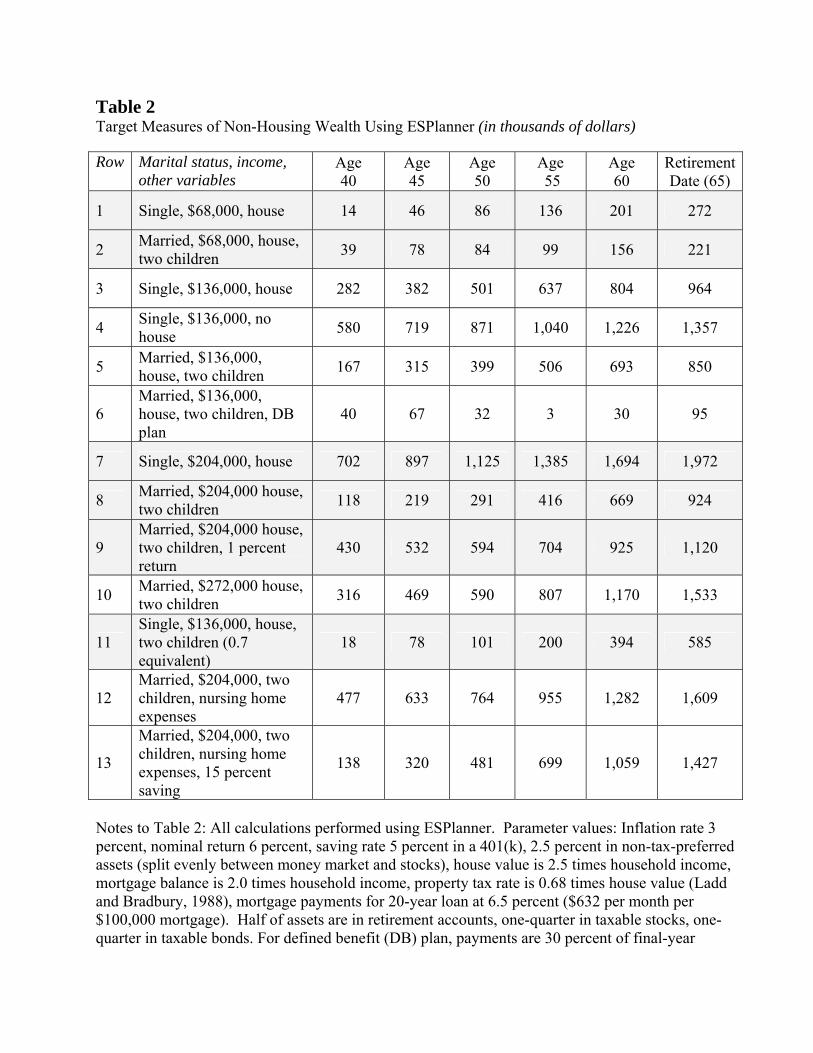
Table 2 Target Measures of Non-Housing Wealth Using ESPlanner (in thousands of dollars)

Notes to Table 2: All calculations performed using ESPlanner. Parameter values: Inflation rate 3 percent, nominal return 6 percent, saving rate 5 percent in a 401(k), 2.5 percent in non-tax-preferred assets (split evenly between money market and stocks), house value is 2.5 times household income, mortgage balance is 2.0 times household income, property tax rate is 0.68 times house value (Ladd and Bradbury, 1988), mortgage payments for 20-year loan at 6.5 percent ($632 per month per $100,000 mortgage). Half of assets are in retirement accounts, one-quarter in taxable stocks, one-quarter in taxable bonds. For defined benefit (DB) plan, payments are 30 percent of final-year

Row Marital status, income, other variables

Age 40

Age 45

Age 50

Age 55

Age 60

Retirement Date (65)

1 Single, $68,000, house 14 46 86 136 201 272

2 Married, $68,000, house, two children 39 78 84 99 156 221

3 Single, $136,000, house 282 382 501 637 804 964

4 Single, $136,000, no house 580 719 871 1,040 1,226 1,357

5 Married, $136,000, house, two children 167 315 399 506 693 850

6 Married, $136,000, house, two children, DB plan

40 67 32 3 30 95

7 Single, $204,000, house 702 897 1,125 1,385 1,694 1,972

8 Married, $204,000 house, two children 118 219 291 416 669 924

9 Married, $204,000 house, two children, 1 percent return

430 532 594 704 925 1,120

10 Married, $272,000 house, two children 316 469 590 807 1,170 1,533

11 Single, $136,000, house, two children (0.7 equivalent)

18 78 101 200 394 585

12 Married, $204,000, two children, nursing home expenses

477 633 764 955 1,282 1,609

13

Married, $204,000, two children, nursing home expenses, 15 percent saving

138 320 481 699 1,059 1,427

31

income. The home mortgage is assumed paid off by age 60. Two children age 8 and 10 at age 40, equivalence scales for children are 0.25 (as in Attanasio, et. al., 1998), $20,000 per year of college expenses in 2006 dollars for incomes of $136,000 or more, $10,000 per year for the $68,000 income household. In the medical expenses scenario, tax-deductible out-of-pocket expenditures for a nursing home stay for the last 5 years of spouse’s life; assumed to be $40,000 annually (in 2006) but in each year such costs rise at a 3% real annual rate, so that by 2056 they are $175,000 for each of the five years. The household is assumed to reside in Pennsylvania for state tax purposes. Single scenario: Single, life expectancy of 95. Married scenario: Equivalence scale of 0.6 for spouse, life expectancy of male is 85, life expectancy of female is 95, $250,000 held in a term life insurance policy.

02

46

8W

ealth

-to-In

com

e R

atio

0 .02 .04 .06 .08 .1Real Interest Rate

Figure 1 The Impact of the Interest Rate on Required Life Cycle Wealth Accumulation Note: This graph shows how changes in assumptions about future real interest rates affect target wealth values to ensure consumption smoothing, evaluated at age 50. The model is as described in the notes to Table 1. The association between the interest rate and wealth-income ratios are shown for different replacement rates of retirement income relative to pre-retirement income: β= 0.2 (20 percent of pre-tax income) , 0.4, and 0.6.

β = .2 β = .4 β = .6

33

0

1

2

3

4

5

6

7

8

HS Dropout HS+ College College+

Education

Wea

lth/In

com

e R

atio

Net Wealth Net Wealth Less House Equity

Figure 2 Wealth-Income Ratios by Education Group: Early Baby Boomers (51-55) in 2004 Source: Calculations by Annamaria Lusardi based on the 2004 Health and Retirement Study (HRS) sample as defined in Lusardi and Mitchell (2006). The bars show median wealth-to-income ratio by income category, and the brackets denote the interquartile range (25th to 75th percentile distribution). N = 2631.

Age T

Earnings/Transfers, Consumption

Consumption

Earnings

Retirement

Retirement Transfers

Utility (Z)

Utility (Z)

Figure 3 Household Production Model: Leisure and Contemporaneous Utility (Z) Rises at Retirement, Consumption Declines Note: Utility Z is a function of consumption and leisure. Because leisure rises so much at retirement, Z jumps up despite the decline in market expenditures or “consumption.” Note that for other parameters of the household production function, consumption may actually rise optimally at retirement.

35

Figure 4 Out-of-Pocket Medical Expenditures as a Percentage of Before-Tax Household Income, Age 75-84, in 1993, 2004, and 2019 (Predicted) Note: N = 1,728 (1993), and N = 1,954 (2004 and predicted 2015). All dollar amounts adjusted by the GDP deflator, and estimated using population weights. Observations excluded if household income is less than $5,000 in 2004 dollars. The 2004 measure asked about the past two years of spending, so one-half the reported amount is presented. For the prediction, a real growth rate of 1.2 percent for income, and 4.0 percent for out-of-pocket expenditures, are assumed, with the latter based on Catlin et al. (2007).

0

0.1

0.2

0.3

0.4

0.5

0.6

0.7

0.8

0.9

< 10% 10-25% 25-50% > 50%

Out-of-Pocket Expenses (% of Income)

Freq

uenc

y

1993 2004 2019 (Predicted)