Are Trade Liberalizations a Source of Global

Imbalances?

Jiandong Ju∗ and Shang-Jin Wei∗∗

June 17, 2010Preliminary and Incomplete

Abstract

A wave of trade liberalizations have taken place in both developing and

developed countries in the last two decades. Global capital flows and the

so-called global imbalances have also risen to an unprecedented level. Are

the two developments related? We study how trade reforms affect capital flows

in a modified Heckscher-Ohlin framework that incorporates convex costs of

capital flows, factor adjustment costs, and financial institutions. We show

that goods trade and capital flows are substitutes in most cases. Since the

nature of trade liberalizations is inherently asymmetric between developed and

developing countries, we show that trade reforms could induce cross-country

capital flows in a way that could contribute to global imbalances.

JEL Classification Numbers: F3 and F4

∗University of Oklahoma, Tsinghua University, and Center for International Economic

Research; E-mail: jdju@ou.edu. **Columbia Business School, NBER, CEPR and CIER, E-mail:

shangjin.wei@columbia.edu, Web page: www.nber.org/∼wei.

0

Contents

1 Introduction 2

2 The Model 4

2.1 Household . . . . . . . . . . . . . . . . . . . . . . . . . . . . . . . . . 5

2.2 Production . . . . . . . . . . . . . . . . . . . . . . . . . . . . . . . . 6

3 Equilibrium Analysis 7

3.1 Heckscher-Ohlin Model with Capital Flows . . . . . . . . . . . . . . 7

3.2 Specific Labor . . . . . . . . . . . . . . . . . . . . . . . . . . . . . . . 9

3.3 Specific Capital . . . . . . . . . . . . . . . . . . . . . . . . . . . . . . 11

3.4 Partial Rigidities . . . . . . . . . . . . . . . . . . . . . . . . . . . . . 13

4 Financial Institutions and Structures of Capital Flows 16

4.1 Determinants of Financial Interest Rates . . . . . . . . . . . . . . . . 20

4.2 Financial Capital Flow and FDI . . . . . . . . . . . . . . . . . . . . 20

4.3 Comparative Statics . . . . . . . . . . . . . . . . . . . . . . . . . . . 21

5 Conclusion 23

6 Appendix 23

1

1 Introduction

A wave of trade liberalizations have taken place in both developing and developed

countries in the last two decades. Global capital flows and global imbalances

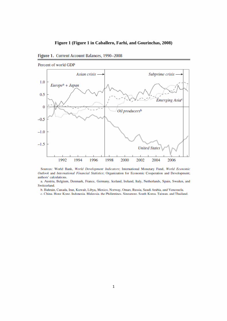
have also risen to an unprecedented level. Figure 1 (from Caballero, Farhi, and

Gourinchas (2008)) displays the main patterns of global imbalances since 1990.

Starting in 1991 the U.S. current account deficit worsened continuously, reaching

6.4 percent of U.S. GDP in the fourth quarter of 2005, then falling back to 5 percent

of GDP by early 2008. The current account surpluses that were the counterpart

of the U.S. deficits initially emerged in Japan and Europe and were bolstered by

surpluses in emerging Asia and the commodity-producing countries after 1997.

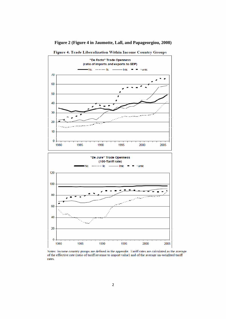
Figure 2 (Figure 4 in Jaumotte, Lall, and Papageorgiou (2008)) illustrates the

wave of trade liberalizations. World trade, measured as the ratio of imports plus

exports over GDP, has grown five times in real terms since 1980. All groups of

emerging market and developing countries, when aggregated by income group, have

been catching up with or surpassing high-income countries in their trade openness.

In particular, the ratio of imports and exports to GDP in low income countries has

increased from about 20% in 1990 to more than 40%, and the average tariff rate in

low income countries has declined from about 60% to 15%. Figure 3 shows balances

of current account in China. China joined the WTO in 2001. The current account

balance was 7.6 billion dollars from 1982 to 2001, but increased to 156 billion dollars

from 2002 to 2007: a 20 times jump!

This paper aims to develop a theoretical model to explain the data patterns

indicated above. In particular, we study how trade reforms affect capital flows in a

modified Heckscher-Ohlin framework that incorporates convex costs of capital flows,

factor adjustment costs, and financial institutions. We show that if a developing

(labor abundant) country reduces the tariff in the capital intensive sector, the

interest rate declines. As a result, capital flows out so that trade liberalizations

2

in a labor abundant country lead to current account surplus. On the other hand,

tariff reductions in the labor intensive sector in a capital abundant country lead to

a decrease in the wage rate but an increase in the interest rate. As a result, capital

flows into the country so that trade liberalizations in a capital abundant country

lead to current account deficits.

Two main problems exist in the classical Heckscher-Ohlin-Samuelson framework

when both goods trade and capital flows are considered. First, As Mundell (1957)

argues, goods trade and capital flow are perfect substitutes in the HO model.

Without costs of trade in goods or capital, there are infinite combinations of goods

trade and capital flow composition that constitute equilibria. So the exact amount

of capital flows is indeterminate. With linear costs of trade in goods and/or capital,

the corner solutions occur: either goods trade or capital flow takes place, but goods

trade and capital flow do not coexist.1 Second, if factors are freely mobile across

sectors, goods trade and capital flow are substitutes. If factors are sector-specific,

however, as Markusen (1983) and Antras and Caballero (2009) point out, goods

trade and capital flow are complement.

By introducing convex costs of capital flows to the Heckscher-Ohlin framework,

we show that there is a unique equilibrium in which goods trade and capital flows

coexist. With factor adjustment costs across sectors, the HOmodel and the factor-specific

model become two polar cases in our model. Thus, the issue of substitutability or

complementarity between goods trade and capital flows can be examined comprehensively.

Suppose a labor abundant country reduces the tariff in the capital intensive

sector. When the capital adjustment cost is small, we show that the tariff cut leads

to lower returns to capital and therefore capital outflows in both sectors. Therefore,

trade liberalizations and capital flows are substitutes in this case. When the labor

adjustment cost is small, the tariff cut always results in lower returns to capital in

the importing sector. The effect on the return to capital in the exporting sector,

1For more detail discussions, readers are guided to Ju and Wei (2007).

3

however, varies with the capital adjustment cost. If the capital adjustment cost is

small, the return to capital in the exporting sector is lower, but becomes higher

when the capital adjustment cost is above a threshold value. In the extreme case,

when labor is freely mobile across sectors, but capital is sector specific, a tariff

reduction results in a decrease in the return to capital in the importing sector,

but an increase in the return to capital in the exporting sector. However, the

average return to capital for all sectors are always lower than that before the trade

reform. Therefore, trade liberalizations and capital flows are substitutes on average.

The theoretical results in this paper, that trade liberalizations in labor abundant

countries lead to the current account surplus, are consistent with the data patterns

of global imbalances we have observed.

We then introduce financial institutions into the model and consider two types of

capital flows: financial capital flow and FDI. We show that trade liberalizations in a

labor abundant country lead to capital outflows in both financial capital and FDI. So

trade liberalizations and two types of capital flows are all substitutes. However, the

effects of financial development on financial capital flow and FDI are opposite: the

higher level of financial development in the country leads to more financial capital

inflow but more FDI outflow.

If trade liberalizations may not balance the trade, we show one possible solution

to the global imbalances is for emerging economies to improve the technology in the

capital intensive sector, and therefore increases the domestic investment demand.

2 The Model

We develop a comprehensive benchmark model in this section. First, we introduce

a convex cost of capital flows so that there is an unique equilibrium in which

goods trade and capital flows coexist. Second, we introduce both labor and capital

adjustment costs so that the HO models and the factor specific models become

4

special cases of out model. In section 4, we further introduce the financial system

to the benchmark model and study how the efficiency of financial system affects

capital flows. To simplify the analysis, we focus on the case of small open economy

in this section.

2.1 Household

The economy’s endowment consists of labor and capital stock which are owned

by households. There are two sectors in the economy. The households supply labor

and capital to both sectors. However, the factors can not be costlessly reallocated

between two sectors. To model the factor market friction, we assume that the

households are subject to quadratic labor and capital adjustment costs for working

in each sector. That is, if the households supply to sector for = 1 2, they

will bear the adjustment costs2( − )

2 and2( −)

2, where and

are parameters that measure the labor and capital market frictions in sector , and

and are labor and capital usages before the trade liberalization, respectively.

As a result, the wage and rental rates will be different across sectors. The wage

rate and the return to capital (the interest rate) in sector are represented by

and , respectively. Let and be the quantity of consumption and the price in

sector The representative consumer’s utility function is (1 2) and she solves

the following maximization problem:

max

(1 2) (1)

subject to

5

11 + 22 +

2X=1

2( − )

2 +

2X=1

2( −)

2 =

2X=1

( + ) (2)

1 + 2 = (3)

1 +2 = (4)

Solving the first order conditions of the above problem, we obtain:

1 = 1 +1 − 2

2 2 = 2 − 1 − 2

2(5)

1 = 1 +1 −2

22 = 2 − 1 −2

2(6)

2.2 Production

Both goods and capital are tradable, while labor is immobile across the border.

The market is perfectly competitive. The production function for good is =

() where measures labor productivity in sector . = can be

understood as effective labor. All production functions are assumed to be homogeneous

of degree one. The unit cost function for is

(

) = min{ + | () ≥ 1}

= min{µ

¶ + | () ≥ 1} (7)

Free entry ensures zero profit for producers. If the country’s endowment is within

the diversification cone, both goods are produced, and we have:

1 = 1(11 1) and 2 = 2(22 2) (8)

6

where is the price of good Let ∗ be the world price,2 and be the tariff rate

in good . Then we have = (1 + ) ∗

3 Equilibrium Analysis

We will first consider two polar cases: the HO model where factors are freely

mobile across sectors, and the specific factor models where either labor or capital

is sector-specific. In the HO model, the parameters that measure factor adjustment

costs, and are set to zero. The wage and the interest rates in two sectors

are equalized and are denoted as and respectively. When labor (or capital)

is sector-specific, on the other hand, (or ) is infinity, so labor (or capital)

employed in sector is fixed. We then move to the general case where and

are between zero and infinity.

3.1 Heckscher-Ohlin Model with Capital Flows

Let e be the amount of capital flow. e 0 denotes capital inflow while e 0

denotes capital outflow. The marginal cost of capital flow is represented by ewhere is a positive number. Thus, the cost of capital flow is assumed to be convex

so that the marginal cost of capital flow is increasing. The equilibrium condition for

capital flows is written as follows:

−∗ = e ⇔ e =−∗

(9)

When ∗ e 0 so capital flows into the country; when ∗ e 0 so

capital flows out.

2We use a superscript “*” to denote variables in the foreign country.

7

The full employment conditions for labor and capital, respectively, are

11 + 22 = (10)

11 + 22 = + e (11)

where

=()

and =

()

(12)

are labor and capital usages per unit of production, respectively.

Let sector 1 be labor intensive. That is, 11

22

In equations (8), we

have 1 = 2 = and 1 = 2 = in HO model. In this HO model, the

Stolper-Samuelson theorem holds. That is, an increase in the price of a good will

increase the return to the factor used intensively in that good, and reduce the

return to the other factor. More formally, we have 1

0, 1

0, 2

0, and

2

0 Note that in our small country model, the increase in price is qualitatively

equivalent to the improvement in technology in equations equations (8). Thus,

we also have 1

0, 1

0, 2

0, and 2

0

Trade liberalizations are represented by reductions in tariffs, 1 and 2 A tariff

reduction in labor intensive sector (a decrease in 1) increases since1

0 Thus,

using equation (9), the amount of capital inflow (outflow) increases (decreases). As

+ e increases, using the Rybczynski theorem, the output of capital intensive

sector, 2 increases relative to 1 so that the country exports more the capital

intensive good. On the other hand, A tariff reduction in 2 reduces and therefore

results in capital outflow. Using the Rybczynski theorem again, the country produces

less 2 relative to 1 so it imports more capital intensive good. Summarizing the

results, we have:

Proposition 1 Suppose factors are freely mobile across sectors. If a country reduces

the tariff in the labor intensive sector, it will export more the capital intensive good

8

but export less capital. On the other hand, if a country reduces the tariff in the

capital intensive sector, it will import more the capital intensive good but import

less capital.

A labor abundant country imports the capital intensive good in the HO model.

Trade liberalizations in the country, therefore, feature a tariff reduction in the capital

intensive sector, which promotes imports of the capital intensive good, but reduces

the interest rate and therefore leads to more (less) capital outflow (inflow). In other

words, trade liberalizations in a developing (labor abundant) country result in more

current account surpluses. By contrast, trade liberalizations in a developed (capital

abundant) country increases the interest rate and therefore result in more current

account deficits.

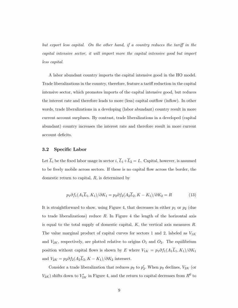
3.2 Specific Labor

Let be the fixed labor usage in sector 1+2 = . Capital, however, is assumed

to be freely mobile across sectors. If these is no capital flow across the border, the

domestic return to capital, is determined by

11(111)1 = 22(22 −1)2 = (13)

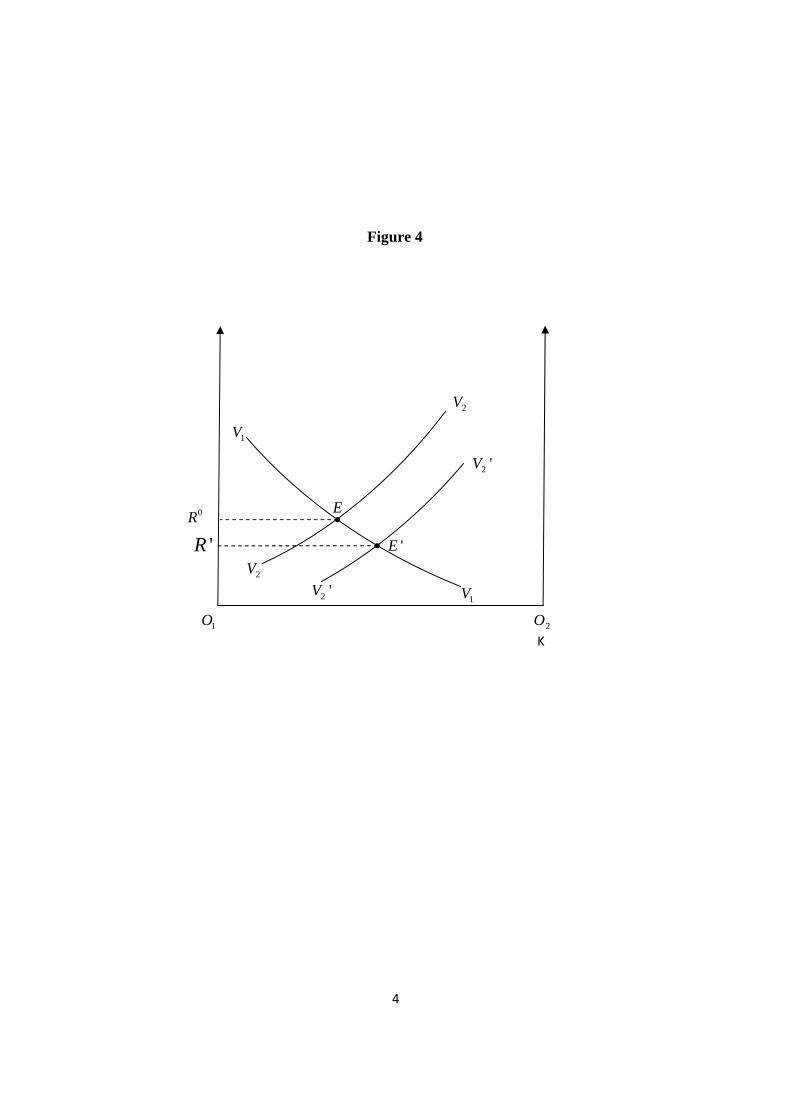
It is straightforward to show, using Figure 4, that decreases in either 1 or 2 (due

to trade liberalizations) reduce In Figure 4 the length of the horizontal axis

is equal to the total supply of domestic capital, the vertical axis measures .

The value marginal product of capital curves for sectors 1 and 2, labeled as 1

and 2 respectively, are plotted relative to origins 1 and 2. The equilibrium

position without capital flows is shown by where 1 = 11(111)1

and 2 = 22(22 −1)2 intersect.

Consider a trade liberalization that reduces 2 to 02 When 2 declines, 2 (or

2) shifts down to 02 in Figure 4, and the return to capital decreases from 0 to

9

0. Likewise, a decline in 1 shifts down 1 and correspondingly reduces It is

interesting to note the difference between HO model and the specific-labor model.

In the HO model, the decrease in 2 reduces but the decrease in 1 increases

while in the specific-labor model, both decreases in 1 and 2 reduce

With capital flows across the border, the equilibrium condition after the trade

liberalization becomes:

011(111)1 = 22(22 + e −1)2 =

−∗ = e (14)

Three endogenous variables,1 e and are solved by the system (14). Summarizing

we have:

Proposition 2 Suppose labor is sector specific, but capital is freely mobile across

sectors. A tariff reduction in any sector reduces the return to capital. As the result,

the country experiences a capital outflow (current account surplus).

Comparing Proposition 2 with Proposition 1, it is interesting to note that for a

labor abundant country, a trade liberalization (reduction in 2) leads to a decrease

in the return to capital, and therefore a capital outflow in both the HO model and

the specific-labor model. However, a trade liberalization (reduction in 1) in a capital

abundant country leads to an increase in and therefore a capital inflow in the HO

model, but a reduction in and therefore a capital outflow in the specific-labor

model.

Two effects are associated with trade liberalizations. First, the decrease in price

reduces the value marginal product of capital, which is labelled as the price effect.

Second, the trade liberalization results in changes in production structures and leads

the country to produce more goods that use its abundant factor intensively, which

is called the structural effect. The former reduces in any country. The later, on

10

the other hand, increases the demand for capital in a capital abundant country and

therefore raises , but decreases it in a labor abundant country.

Both the price effect and the structural effect reduce the return to capital in a

labor abundant country, so a trade liberalization leads to capital outflow in the HO

model and in the specific-labor model. However, the structural effect is weaker in

the specific-labor model, as immobile labor prevents the structural adjustment at

the full scale. Thus, the reduction in and therefore the amount of capital outflow

in a labor abundant country is smaller in the specific-labor model than that in the

HO model. On the other hand, however, the price effect and the structural effect

move in opposite directions in a capital abundant country. Furthermore, in HO

model the later dominates the former, so a trade liberalization leads to a capital

inflow, while in the specific-labor model, it is the reverse.

3.3 Specific Capital

Let be the fixed capital usage in sector Now labor is assumed to be freely

mobile across sectors. Without capital flow across the border, the wage rate is

determined by

11(111)1 = 22(2 (− 1) 2)2 = (15)

Similar to the above analysis, the wage rate declines after the trade liberalization.

Consider a decrease in 2 Similar to the analysis in Figure 4, but now the the

horizontal axis represents the supply of labor, and the vertical axis measures the

wage rate . As a result of the decrease in 2 the value marginal product of labor

curve for sector 2, 2 = 22(222)2 shifts down. So 2 decreases. Both

decreases in 2 and 2 reduce the return to capital in sector 2, 2 = 22(222)2

Thus, the decrease in 2 leads a capital outflow in the importing sector 2. On the

other hand, the decrease in 2 implies that 1 increases. Therefore, the return to

11

capital in sector 1, 1 = 11(111)1 must increase, which leads to a

capital inflow in sector 1. Likewise, if a tariff reduction results in a decrease in 1,

then 1 declines but 2 increases. Summarizing we have:

Proposition 3 Suppose capital is sector specific, but labor is freely mobile across

sectors. A tariff reduction results in a decrease in the return to capital in the

importing sector, but an increase in the return to capital in the exporting sector.

As a result, the country experiences a capital outflow in the importing sector but a

capital inflow in the exporting sector.

The effects of trade liberalizations on capital flows can be summarized as follows.

Table 1

Labor Abundant Country Capital Abundant Country

Tariff Reductions 2 ↓ 1 ↓HO ↓ ↑

Specific Labor ↓ ↓Specific Capital 1 ↑ 2 ↓ 1 ↓ 2 ↑

Antras and Caballero (2009) argue that trade liberalizations and capital flow are

complements, in the sense that a process of trade integration increases the incentives

for capital to flow to developing country. From the above table, only one case in our

analysis that if capital is sector specific, and capital in sector 2 is prohibited to flow

across the border, then trade liberalizations and capital flow are complements. This

case bears some similarity to the case discussed by Antras and Caballero (2009)

where capital in sector 2 is fixed due to financial frictions and capital in sector 2

(called entrepreneurs’ capital) is not allowed to flow across the border. In this case,

trade liberalization in the developing country expands the country’s production in

sector 1, and therefore induces foreign capital to flow into the sector.

12

It is interesting to note that the complementarity between trade liberalizations

and capital flows discussed by Antras and Caballero (2009) is rather special in our

discussions. If factors are freely mobile (HO model), or labor but not capital is

sector specific, we all have that trade and capital flows are substitutes, rather than

complement. The effect of financial development on capital flows, which is a focus

in Antras and Caballero (2009), will be discussed in section 4.

3.4 Partial Rigidities

We now discuss the general case that both labor and capital are partially rigid.

That is, the adjustment cost parameters, and are between zero and infinity.

The model with general function forms is complicated and we do not have a closed

form solution to the comparative statics. So we parameterize the model and use

simulations to analyze the effect of factor market rigidities on capital flows.

We assume the following Cobb-Douglas production functions

1(111) = (11)1 1−1

1 and 2(222) = (22)2 1−2

2 (16)

Thus, we have

=()

=

1− (17)

=()

= (1− )

− (18)

where =

Using (5) and (6), we obtain:

1 =1 +

1−11 −2

−22

2

1 +1

1−11 −2

1−22

2

(19)

2 =2 − 1

−11 −2

−22

2

2 − 11−11 −2

1−22

2

(20)

13

where = and = (1− )

Equations (19) and (20) solve for

1 and 2 which than solve for the wage rates and the returns to capital, using (17)

and (18). Let be the marginal cost of capital flow in sector to across the border.

Similar to equation (9), capital flows across the border in two sectors, respectively,

are determined by the following equations:

e1 =1 −∗

1 e2 =

2 −∗

2(21)

Finally, the factor usages and in each sector are solved by four equations as

follows.

1

1= 1

2

2= 2

1 + 2 = and 1 +2 = + e1 + e2

We set the parameters in the model as follows:

1 = 075 2 = 025

∗1 = 9 ∗2 = 1

1 = 0 2 = 02

∗1 = 0 ∗2 = 0

∗ = 153867 ∗ = 019

1 = 1 2 = 0482

∗1 = 1 ∗2 = 1

= 1 = 135

1 2 so sector 1 is labor intensive. The home country is labor abundant and

exports good 1 before the trade reform. Let the tariff rate be zero in sector 1, and

20% in sector 2 at home. Thus the prices at home are 1 = 9 and 2 = 12 1 is

set to 1. 2 is chosen so that 222 = 1 Assume that the foreign country imposes

14

zero tariffs. Thus = ∗

∗ The economy is in the steady sate equilibrium

before the reform and adjustment costs are zero. So we must have 1 = 2 =

and 1 = 2 = Using (17) and (18), therefore, factor prices at home and abroad

are equalized, so there is no capital flow before the reform.

Using equations (17) and (18), we have the solution 1 = 27 and 2 = 243 That

gives = 153867 = ∗ and = ∗ = 019 Let 1 = 2 = 12 1 = 272 and

2 = 2432 which implies that = 1 and = 135

Now consider a tariff cut which reduces 2 to zero. After the reform 1 =

∗1111 = 675 2 = ∗22

22 = 0208 1 = ∗1 (1− 1)

11 = 225 and

2 = ∗2 (1− 2)22 = 0625 Using these results, we then solve for 1 and 2 by

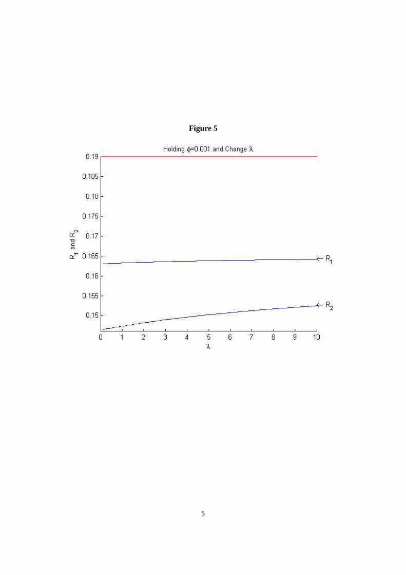
equations (19) and (20). To examine the effect of factor market rigidities, we first

fix the capital adjustment cost = 0001 and let change from 01 to 10 The

results are reported in Figure 5. The 20% tariff cut in sector 2 reduces 1 to below

01642 and 2 to below 01524 That is, the tariff cut reduces the interest rate by

more than 019−01642019

= 136% in sector 1, and more than 019−01524019

= 198% in

sector 2. When increases from 01 to 10 both 1 and 2 increase, reflecting that

as the labor market becomes more rigid, less labor intensive good is produced and

the domestic demand for capital is higher.

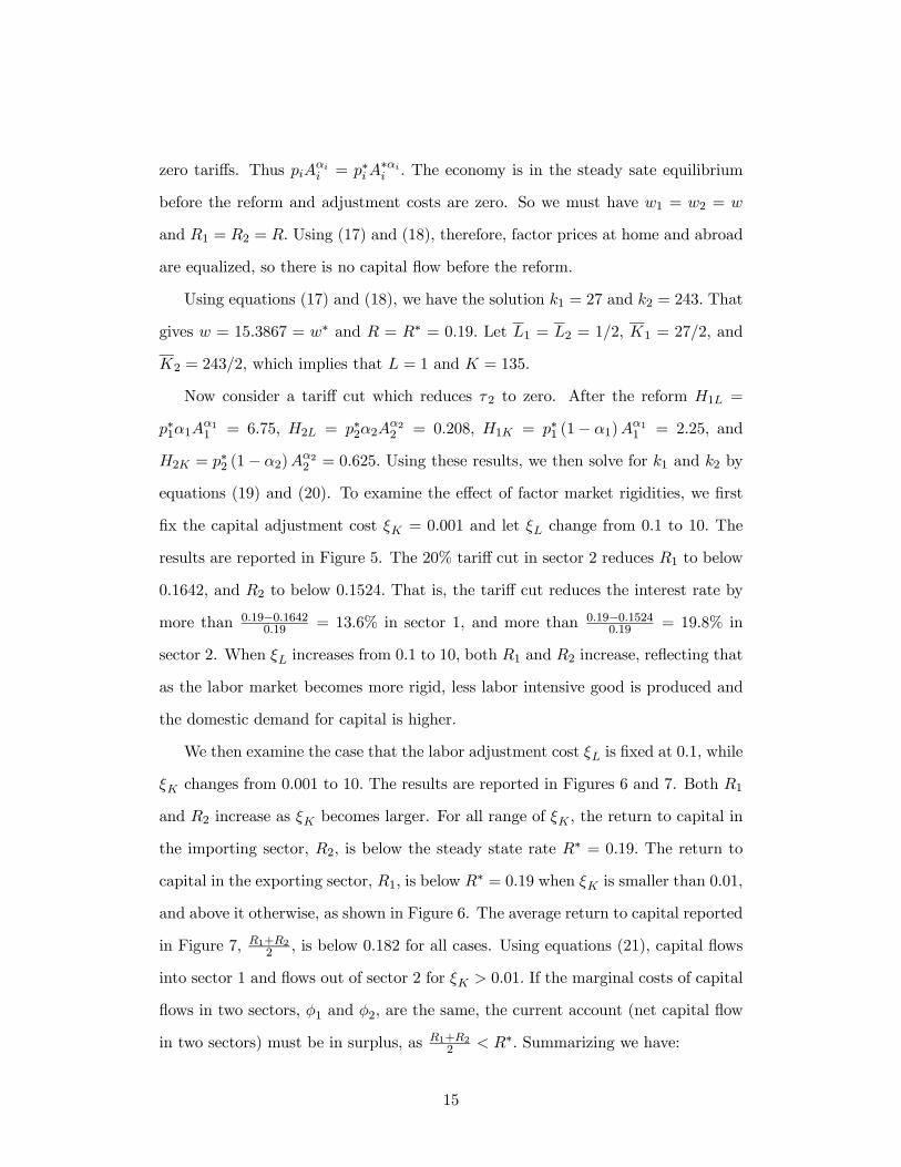
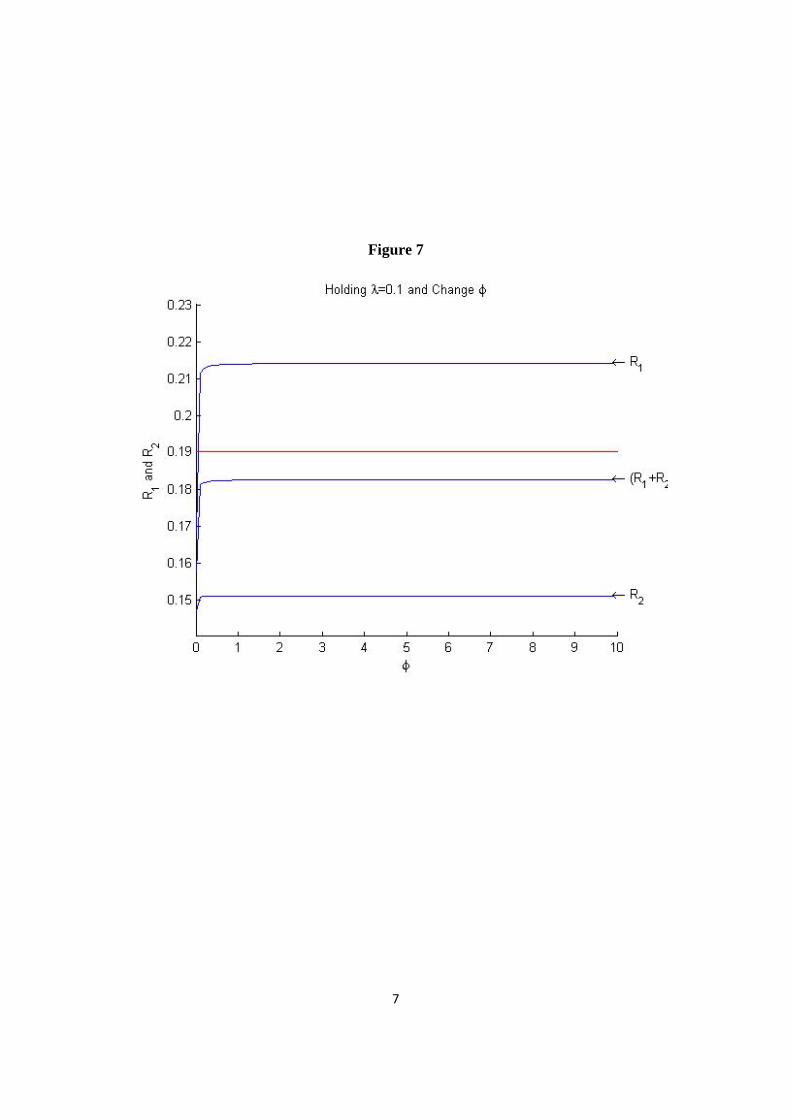
We then examine the case that the labor adjustment cost is fixed at 01, while

changes from 0001 to 10 The results are reported in Figures 6 and 7. Both 1

and 2 increase as becomes larger. For all range of the return to capital in

the importing sector, 2 is below the steady state rate ∗ = 019 The return to

capital in the exporting sector, 1 is below ∗ = 019 when is smaller than 001

and above it otherwise, as shown in Figure 6. The average return to capital reported

in Figure 7, 1+22

is below 0182 for all cases. Using equations (21), capital flows

into sector 1 and flows out of sector 2 for 001 If the marginal costs of capital

flows in two sectors, 1 and 2, are the same, the current account (net capital flow

in two sectors) must be in surplus, as 1+22

∗ Summarizing we have:

15

Proposition 4 Suppose a labor abundant country reduces its tariff in the capital

intensive sector. A) The tariff cut always results in lower return to capital in

the importing sector. B) If the capital adjustment cost is sufficiently small, the

tariff cut also leads to lower return to capital in the exporting sector; if the capital

adjustment cost is above a threshold, however, the return to capital in the exporting

sector becomes higher. On average, the return to capital is lower than that before

the reform. C) As factor adjustment costs across sectors become larger, the return

to capital increases.

4 Financial Institutions and Structures of Capital Flows

In this section we introduce the financial contract into the model discussed above.

The financial contract model is based on Ju and Wei (2008) who incorporate the

financial contract model of Holmstrom and Tirole (1997) into the standard Heckscher-Ohlin

framework. The model in this paper differs from that in Ju and Wei (2008) as we

allow the private benefit to entrepreneurs to be endogenous in this paper.

Suppose the production process takes two periods. The capital endowment

in the country is owned by number of capitalists, each born with 1 unit of

capital and facing an endogenous choice of becoming either an entrepreneur or a

financial investor at the beginning of the first period. If a capitalist chooses to be an

entrepreneur, she would manage one project, investing her 1 unit of capital (labeled

as internal capital) and raising amount of additional capital (external capital)

from financial investors in sector , possibly through a financial institution. The

total investment in the firm in sector is the sum of internal and external capital,

or = 1 + . There will be = of firms in sector

After the investment decision is made in the first period, production and consumption

take place in the second period. Let depreciation rate be zero. If the project

succeeds, the gross return to one unit of capital in sector is which is the value

16

marginal product of capital discussed in the above sections. The financial interest

rate received by investors is denoted as Note that if capital is freely mobile across

sectors, 1 = 2 =

For a representative firm, the final output depends in part on the entrepreneur’s

level of effort, which can be low or high, but is not observable by the financial

investors or the financial institution. Assume that the entrepreneur can choose

among two versions of the project. The “Good” version has a high probability

of success, while offering no private benefit. The “Bad” version has a lower

probability of success, but offering a private benefit per unit of capital managed,

to the entrepreneur. Following Holmstrom and Tirole (1997), we further assume

that only the “Good” project is economically viable. That is, −(1 + ) 0

− (1 + ) + so that only the “Good” project is implemented in the moral

hazard problem.

We use to denote a country’s level of property rights protection, where (1− )

could be understood as a tax rate on the capital returns, where taxation is broadly

defined to include state expropriation. We normalize = 0 and define =

thereafter. Since we fix , without loss of generality, we can conveniently refer to

directly as an index of property rights protection.

The entrepreneur is paid per unit of capital to induce her to choose the

“Good” project. In addition to that, we assume that units of numeraire good

are used to intermediate one unit of investment in sector . Thus, the pay to the

financial intermediation is units of good per unit of investment. may

represent the transaction cost, the monitoring cost to reduce the extent of moral

hazard, or the expropriation by government officials. The efficiency level of the

financial system in the country is then represented by . The higher the , the

lower is the financial intermediation cost.

The entrepreneur in sector chooses the amount of external capital her own

capital contribution to the project , total investment of the project and the

17

marginal pay to the entrepreneur’s effort to solve the following program:

max

= + (1 + ) (1− ) (22)

subject to

≤ 1 (23)

≤ + (24)£¡ −

¢− ¤ ≥ (1 + ) (25)

≥ (26)

The objective function (22) represents the entrepreneur’s expected income. The

first term represents the entrepreneur’s share in total capital revenue. The second

term is the return from investing her own 1 − capital in the market. Turning

into the constraints, inequality (23) requires that entrepreneur’s internal capital is

less than her capital endowment. Inequality (24) requires that total investment

does not exceed the sum of internal and external capitals. Inequality (25) is the

participation constraint for the outside financial investors,3 while inequality (26) is

the entrepreneur’s incentive compatibility constraint.

It is then straightforward to show that all constraints must be binding in equilibrium.4

The entrepreneur will invest all her endowment = 1 in the firm. The total

investment equals the sum of internal and external capitals + 1 The incentive

compatibility constraint (26) gives

=

(27)

3Following Holmstrom and Tirole (1997), it is assumed that financial intermediaries monitor

entire project to ensure entrepreneurs to behave. Thus, the intermediation cost is proportional to

the amount of total capital, not just external capital.4The problem is solved by setting the Lagrangian. The marginal return to internal capital

must be higher than the financial interest rate as the entrepreneur needs to pay an entry cost (to be

specified later). Then straightforward manipulation of the first order conditions shows that (23),

(24), (25), and (26) must bind.

18

Substituting (27) into (25) gives the firm’s optimal investment5

=1 +

(1 + ) + + − (28)

Substituting (27) and (28) into (11), the entrepreneur’s expected income becomes

= (1 + )

(1 + ) + + − (29)

We assume that a capitalist (a potential entrepreneur) needs to pay a fixed entry

cost of units of goods to become an entrepreneur.6 With free entry and exit of

entrepreneurs, an entrepreneur’s expected income net of the entry cost −(1+)should be equal to (1 + ) so that capitalists are indifferent between becoming

entrepreneurs or financial investors in equilibrium. That is,

− (1 + ) = (1 + ) (30)

Using (29), the free entry condition (30) implies that

= (1 + ) +

+

1 + (31)

The equation (31) describes how the expected return to the physical capital is

divided up among its usages, which we label as a capital revenue sharing rule. The

expected marginal product of capital on the left hand side of the equation, is shared

by the return to financial investment, 1 + the cost of financial intermediation,

and the agency cost 1+

paid to the entrepreneur.

5Following Holmstrom and Tirole (1997), we rule out the case that (1 + ) + + − 0

in which the firm would want to invest without limit.6Both intermediation costs, and the enty cost, are in the unit of numeraire good which

has the same function form as the consumer’s utility function.

19

4.1 Determinants of Financial Interest Rates

The financial interest rate, and the private benefit, are solved by capital revenue

sharing rules (31) in sectors 1 and 2. To simplify the analysis, we consider the case

that the capital adjustment cost is zero so that 1 = 2 = Denoting 1+

as

we have:

= − 1− 21 − 12

(2 − 1)(32)

=1 − 2

(2 − 1)(33)

We assume that the fixed cost to become an entrepreneur in capital intensive

sector 2 is higher than that in sector 2, so that 2 1 Furthermore, we assume

that the monitoring cost in sector 1 is higher than that in sector 2. That is, 1 2

Under these assumptions, the private benefit is positive when 1 = 2.7

4.2 Financial Capital Flow and FDI

Let and be the amounts of financial capital flow and FDI, respectively. Recall

that a positive number represents capital inflow and a negative number represents

capital outflow. The marginal costs of financial capital flow and FDI are and

, respectively. Financial capital goes where the interest rate is the highest.

The equilibrium condition for financial capital flow is

− ∗ = (34)

Foreign direct investment (FDI) goes to where the expected return to an entrepreneur

is the highest. It takes place when the entrepreneur decides to take her project (and

the capital under her management) to a foreign country and use foreign labor to

7Alternatively, we may assume that 1 2 and 1 2

20

produce.

We assume that the entrepreneur still uses her native financial system only and

pay the domestic interest rate. In other words, if a U.S. multinational firm operates

in India, the US firm still uses a US bank or stock market for its financing need.

When an entrepreneur at home in sector directly invests in the foreign country

and produces there, using (29), the entrepreneur’s expected income becomes

=

(1 + )

(1 + ) + + − ¡∗∗ + ¢ (35)

In equilibrium, we must have = which holds if and only if

= ∗∗ + (36)

It is easy to verify that condition (36) is also the equilibrium condition for a foreign

entrepreneur to directly invest in the home country.

4.3 Comparative Statics

The return to capital, is determined by product prices and total capital usages

(together with labor productivity, labor endowment, and factor adjustment costs)

in the home country. Thus, we write = (1 2+ +) Substituting (32)

into (34) and rewriting (36), we have:

(1 2 + +)− = 1 +1

µ21 − 12

2 − 1

¶+ ∗ (37)

(1 2 + +)− = ∗∗ (38)

Totally differentiating equations (37) and (38), in the Appendix we show that

0 but

0 while

=

and

=

Thus, as the

efficiency of financial system improves ( increases), there will be more financial

21

capital inflow, but more FDI outflow. Consider trade liberalizations in a labor

abundant country (decrease in 2) and changes in the efficiency of financial system.

We have:

=

22 +

=

22 +

(39)

=

22 +

=

22 +

(40)

When the capital adjustment cost is zero, as we have discussed in Proposition

2, a reduction in 2 decreases the return to capital That is,2

0 Thus, there

will be more (less) outflows (inflows) in both financial capital and FDI. On the other

hand, an improvement in a developing country’s efficiency of financial institutions

(an increase in ), tends to simultaneously reduce its financial capital outflow and

FDI inflow. While an increase in does not directly affect the marginal product of

capital, it leads to a higher financial interest rate in condition (32). As a result,

there is less incentive for financial capital to leave the country. As more financial

capital stays with local firms, the marginal product of capital declines, which makes

it less attractive for inward FDI.

Therefore, trade liberalizations and both financial capital flow and FDI are

substitutes, in the sense that the trade liberalizations in a labor abundant country

lead to less inflows in both financial capital and FDI. It is interesting to note that

different from Antras and Cabellero (2009) which shows that the lower financial

development in South, the lower the amount of trade integration needed (higher

tariff rate) to ensure that capital flows into South, in our model the effect of trade

liberalizations on capital flows is independent from the level of financial development,

as 2

= 2

= 0 Summarizing we have:

Proposition 5 The trade liberalizations in a labor abundant country lead to less

inflows (more outflows) in both financial capital and FDI. The lower financial development

22

in the country leads to more financial capital outflow but more FDI inflow. The effect

of trade liberalizations on capital flows is independent from the level of financial

development.

5 Conclusion

To be written.

References

[1] Antras, Pol and Ricardo J. Caballero (2009), “Trade and Capital Flows: A

Financial Frictions Perspective,” Journal of Political Economy, 117(4), pp.

701-744.

[2] Caballero, Ricardo J., Emmanuel Farhi, and Pierre-Olivier Gourinchas (2008),

“Financial Crash, Commodity Prices, and Global Imbalances,” Brookings

Papers on Economic Activity, Fall, 1-68.

[3] Jaumotte, F., S. Lall, and C. Papageorgiou, 2008, “Rising Income Inequality:

Technology, or Trade and Financial Globalization?” IMF Working Paper

08/185.

[4] Ju, Jiandong and Shang-Jin Wei (2008), “When Is Quality of Financial System

a Source of Comparative Advantage?” NBER Working Paper 13984.

[5] to be added.

6 Appendix

This appendix analyzes the effect of changes in prices and efficiency of financial

system on financial capital flow and FDI. Totally differentiating equations (37) and

(38), we obtain:

µ

−

¶ +

= −

2 −

11 −

22 (41)

+

µ

−

¶ = −

11 −

22 (42)

where = 21−122−1 0 Let Let || denote the determinant of the 2× 2 matrix on

the left hand side of the above system. We can show that

|| = −

−

+ 0 (43)

23

since 0 and

0 It is then easy to show that

= −

2

µ

−

¶ 0

=

2

0

=

and

=

(44)

24

1  

Figure 1 (Figure 1 in Caballero, Farhi, and Gourinchas, 2008)

 

 

 

 

 

 

 

 

 

2  

Figure 2 (Figure 4 in Jaumotte, Lall, and Papageorgiou, 2008)

 

3  

Figure 3

 

 

 

 

 

 

 

 

 

 

 

 

 

 

‐50

0

50

100

150

200

250

300

350

1980

1981

1982

1983

1984

1985

1986

1987

1988

1989

1990

1991

1992

1993

1994

1995

1996

1997

1998

1999

2000

2001

2002

2003

2004

2005

2006

2007

Trade Balance( Billian $)

Trade Balance( Billian $)

4  

 

 

 

0R  

1O  

2 'V  

2V  

1V  

 

'E  

E  

2O  

Figure 4

1V  2 'V  

2V  

 

K

'R  

5  

Figure 5

6  

Figure 6

7  

Figure 7