Are they all crazy or Just Risk Averse? Some Movie Puzzles and Possible Solutions. By S. Abraham Ravid* First Draft, May 2002 Revised June 2002 *Rutgers Business School, Rutgers University, 180 University Av. Newark, NJ 07102 email: ravid@andromeda.rutgers.edu The author wishes to acknowledge many useful discussions with Suman Basuroy and Art DeVany on these issues. All errors remain my own.

Introduction Making profitable movies remains a very elusive goal. Producers use, they say, gut

feeling, heavy promotions and stars in order to somehow hedge uncertain bets.

In this paper we will survey recent work on the nature film profitability and provide some

support for the idea that decisions in the film business are made according to a risk averse

objective function, not necessarily in the best interests of shareholders.

This essentially only moves the puzzle one step back, namely to the question of why such

objective functions are allowed in equilibrium. We can and will speculate on that some.

However, here we are in good company, and we will show that much of the new

literature in finance supports the view that executives in various industries tend not to

take risks or to hedge too often.

The plan of the paper is as follows – we first survey the literature on profitability in

films. This literature suggests that some observed decisions are sub-optimal. We then

survey the literature on non- profit maximizing executive decision. Finally we provide

evidence that seems to support the view that film executives’ decisions follow from risk

averse objective functions.

Profitability Studies.

There have been a few early studies of the determinants of profitability in movies. Litman

(1983) finds that Academy award nominations or winnings are significantly related to

revenues. Smith and Smith (1986) analyze a sample, which includes only the most

successful films in the 50's 60's and 70's. The results (which differ by decade) of running

revenues against awards are curious. For instance, winning an award seems to have a

negative and significant effect in the 60's and a positive and significant effect in the 70's.

The Best Actor award variable is insignificant, whereas the Best Actress award variable

changes sign from positive in the 50's to negative in the 70's. The total number of awards

received per film has a positive and significant effect on revenues.

Litman and Kohl (1989) find that the participation of stars and top directors, critical

reviews, ratings, and several other variables are significantly related to revenues. However,

academy award nominations are significant only for the best film category and winning

does not seem to affect revenues.

These studies, as well as some sophisticated analyses of success in the business (see

Eliashberg and Shugan (1997) and Eliashberg and Sawney (1996)) have focused on

receipts. In recent years, there have been several studies, which have extended earlier

work, added variables and included return on investment. Ravid’s (1999) study is based

upon a sample of close to 200 films in the early 1990’s. It extended the literature in several

ways empirically and conceptually. Conceptually, it sought to explain the importance (or

lack thereof) of stars to economic success, using the competing economic concepts of

signaling (with an expensive star) or rent capture (if stars capture all their value added).

Empirically, in addition to domestic revenues, (which have been the focus of most previous

research), and which currently represent less than 20% of the total receipts of a typical

movie, Ravid (1999) includes video and international revenues. Indeed, it turns out that

video revenues drive one of the most significant conclusions in the study1. Recently, many

films have spawned merchandise and other products, which of course make films more

valuable properties.2 Therefore, the inclusion of additional sources provides a much better

picture of where the money comes from in the industry.

Second, Ravid (1999) uses a comprehensive set of control variables, including MPAA

ratings, sequel status, critical reviews and release dates. The study naturally includes

several alternative star definitions. Also, the study is based upon a random sample, as

opposed to top 100 or other non-neutral classifications, which were common in earlier

work.

Finally, Ravid (1999) also studies the return on investment, rather than just revenues, on

the left-hand side of the equation. This is important, because, most studies find that budgets

1 S&P Credit week (1997) reports that in 1996 video revenues were the largest component of the average film's revenues. This was not yet the case in Ravid (1999) sample period (video revenues have grown about 7 fold between 1986 and 1996); still, the inclusion of video revenues and international theatrical revenues improves the accuracy of our revenue estimate compared to other recent studies.

2"The Lion King", a very successful recent G rated movie, cost $55 million to make in 1994. It took 313 million in domestic theaters, 454 million abroad, 520 million in video revenues, but Disney also sold another 3 billion dollars worth of related merchandise (see Stevens and Grover, 1998).

are a main driver of revenues. Thus, it is easy to produce movies that make a lot of money-

just put in a lot of money. However, that may not be a profit maximizing strategy.

However, in studying profitability, one is faced with many difficulties. First, although most

movie studios are publicly traded companies, they do not have to report individual project

information. Thus, much of the needed data is not public. Further, even if it were, the

nature of movie accounting (and other accounting, as we have learned from Enron..) is such

that profit and loss statements must be pruned essentially line by line if one is to reach

economically meaningful numbers. Thus, even if profit were reported, it would not

necessarily be meaningful.

Thus Ravid (1999) chooses a proxy measure, namely total revenue over negative cost,

which represents a good approximation for profit. Ravid (1999) does not include

advertising and promotional costs, however, his specification implicitly assumes that such

costs are proportional to the budget. Ravid and Basuroy (2002) who later collected these

data for the same sample, found that the conjecture was right – in fact, the correlation was

so high that it was impossible to run these cost components separately in a regression.

Ravid (1999) finds that stars play no role in the financial success of a film. Univariate tests

support the industry view that stars increase revenues. However, in multiple regressions,

including budget figures, budgets seem to take all the significance - in other words, big

budget films may signal high revenues, regardless of the source of spending. Also,

attention by reviewers seems to be important to success - the more reviews a film receives,

the higher the revenues. Film ratings are important as well and sequels seem to do better

which is consistent with the view that insiders are not better informed than outsiders, but

when, for whatever elusive reason, a film succeeds, studios attempt to replicate the

formula.

Return regressions also cannot reject the "rent capture" vs. the signaling hypothesis.

That is to say, stars are not correlated with returns either. However, the role of budgets sees

a dramatic reversal - big budgets do not contribute to profitability - if anything (as the final

table in Ravid (1999) demonstrates) they may contribute to losses. Only G and PG ratings

and marginally sequels or reviewers' attention seem to matter. A later study on a

completely different sample supports the view that budgets on average are bad for returns

(see John Ravid and Sunder (2002)).

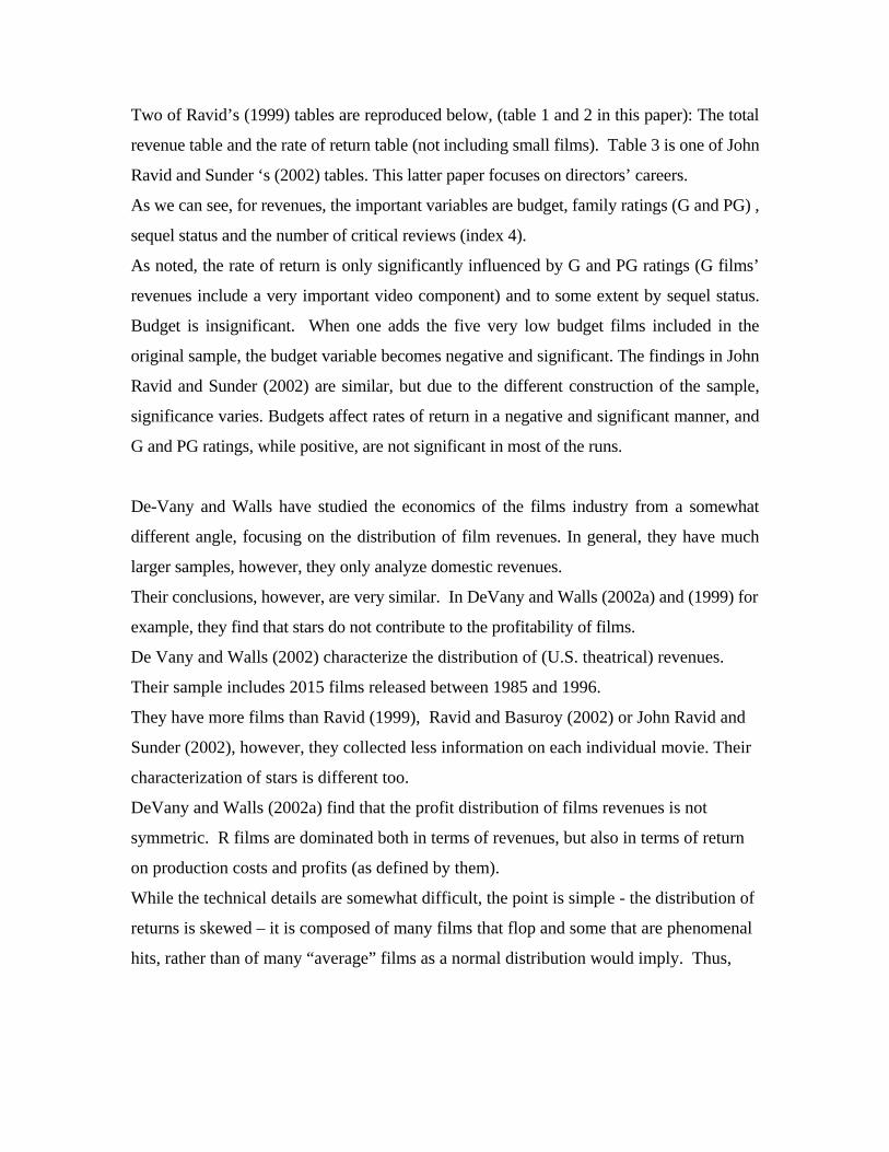
Two of Ravid’s (1999) tables are reproduced below, (table 1 and 2 in this paper): The total

revenue table and the rate of return table (not including small films). Table 3 is one of John

Ravid and Sunder ‘s (2002) tables. This latter paper focuses on directors’ careers.

As we can see, for revenues, the important variables are budget, family ratings (G and PG) ,

sequel status and the number of critical reviews (index 4).

As noted, the rate of return is only significantly influenced by G and PG ratings (G films’

revenues include a very important video component) and to some extent by sequel status.

Budget is insignificant. When one adds the five very low budget films included in the

original sample, the budget variable becomes negative and significant. The findings in John

Ravid and Sunder (2002) are similar, but due to the different construction of the sample,

significance varies. Budgets affect rates of return in a negative and significant manner, and

G and PG ratings, while positive, are not significant in most of the runs.

De-Vany and Walls have studied the economics of the films industry from a somewhat

different angle, focusing on the distribution of film revenues. In general, they have much

larger samples, however, they only analyze domestic revenues.

Their conclusions, however, are very similar. In DeVany and Walls (2002a) and (1999) for

example, they find that stars do not contribute to the profitability of films.

De Vany and Walls (2002) characterize the distribution of (U.S. theatrical) revenues.

Their sample includes 2015 films released between 1985 and 1996.

They have more films than Ravid (1999), Ravid and Basuroy (2002) or John Ravid and

Sunder (2002), however, they collected less information on each individual movie. Their

characterization of stars is different too.

DeVany and Walls (2002a) find that the profit distribution of films revenues is not

symmetric. R films are dominated both in terms of revenues, but also in terms of return

on production costs and profits (as defined by them).

While the technical details are somewhat difficult, the point is simple - the distribution of

returns is skewed – it is composed of many films that flop and some that are phenomenal

hits, rather than of many “average” films as a normal distribution would imply. Thus,

one must worry about the predictive power of data analysis. 3 However, table 5 in their

study shows that only 6% of R rated movies make over 50 million dollars, whereas 13%

of G and PG rated films succeed in doing so, as well as 10% of PG-13 rated films.

Similarly, 20% of G rated films are hits (rates of return more than 3 times the production

budget) as opposed to 16% for PG, 12% for PG 13 and 11% for R rated films.

For G films, the mean lies much to the right of the median. It is true also for other films,

but less so. Thus G films stochastically dominate all others almost everywhere.

Therefore, if we were to summarize the conclusions of these recent profitability studies,

one can say that big budget movies lead to higher revenues, but generally to somewhat

lower returns. Stars do not help or hurt movies. What seems to be important for return on

investment is a G or PG rating and to some extent sequel status.4

The puzzle

This summary leaves us with three major puzzles – first, if indeed stars do not help you out,

why hire them? Industry wisdom talks about “bankable stars”, who can “open” a movie,

and further, very often projects are funded if a star is attached. Does industry simply not

know what is going on? Are they just unaware of all studies or are they just ignoring

them?5

Second, if we believe the consistent finding that G films perform better, why is it that so

few G films are being produced? The puzzle becomes even more pronounced when we

realize that the huge success of G films is not a new or surprising phenomenon – the past is

3 However, the distribution of total revenues is in general smoother than that of domestic revenues, since films may make money in video, internationally or in TV distribution, even if they do not do well domestically. This may make the profit distributions less skewed. For example, the finding that violent movies do well internationally will move the revenue distribution of R films more to the center. 4 Simonoff and Sparrow (2000) use a different sample, films released in 1997-98. Only domestic revenues are considered. However, the G- factor seems to be there, in spite of the fact that the main source of income of G rated films is video revenues (not included in their sample) and that, as we saw international revenues matter. 5 This latter view is probably not true – Ravid (1999) was cited in Variety several times, as well as in the Hollywood Reporter, NY Times Wall Street Journal and papers around the world, and requested by dozens of industry executives.

all about G films. As noted in Ravid (1999), the list of top 10 films of all times (adjusted

for inflation) is dominated by G rated films, including the likes of Bambi and Fantasia.

Table 4 shows the distribution of films by MPAA ratings through the 90’s. The percentage

of R- rated films, which has always been (too?) high has not declined, but has increased

over the years. So, is indeed Hollywood producing too many R-rated movies, as DeVany

and Walls (2002) ask, and if so, why? .6

The third puzzle is Hollywood’s pursuit of so- called “event movies” (Consider Pearl

Harbor or Spiderman as recent examples) which by definition are expensive action-packed

films. If big budgets are not good for you, why not just go for a slate of small films instead?

In the remainder of the paper, we will attempt to provide at least partial answers to this

triple puzzle. In order to do that, one must consider other attributes of the films in question,

namely their risk characteristics. When we do that, we can show that all three puzzles can

be interpreted as risk –minimizing strategies by extremely risk-averse executives. In the

next section we will review the literature on executive objective function. The final section

will show how such objective functions can lead to the puzzles we have described.

Executive objectives – a review

Agency theory, going back to Jensen and Meckling (1976), Holmstorm (1979)

and many other related papers suggests, that when the objective function of the agent is

different from that of the principal, one may observe behavior that deviates from value

maximization (unless it is not too costly to eliminate all such deviations with the proper

use of incentives).

In particular, many papers, going back to Baumol (1958) have described revenue

maximization as a possible goal for firm managers. For example, Fershtman and Judd

(1987) model a case where owners, who are interested in profit maximization, may find it

optimal to include sales maximization in the agent’s objective function in an oligopoly

setting. The general idea is that if one of the two firms modeled maximizes sales, then

the other is better off increasing output rather than keeping output low. Zaboznic (1998)

develops this idea further.

Other studies have sought to justify and document another seeming deviation

from profit or value maximization, namely, corporate hedging behavior. In general,

investors should not want firms to hedge risks, which shareholders can usually hedge

better on their own by portfolio choices and in various derivative markets. However,

specific imperfections can make hedging an optimal policy for an individual business

entity. Smith and Stulz (1985) identify and model three such imperfections, namely,

taxes, bankruptcy costs, and managerial risk aversion. Empirical studies, in particular a

study by Tufano (1996) of the gold-mining industry, seem to show that corporate officers

do engage in hedging. Tufano (1996) finds that almost all firms in the gold mining

industry employ some form of hedging. He detects no correlation between hedging and

measures of bankruptcy costs. However, he does find a significant relationship between

hedging measures and proxies for risk exposure of executives. Tufano (1996) also tests

several other theories.

A well-known paper by Froot et al. (1993) justifies hedging as a way of avoiding

costly external financing. Thus hedging enables the firm to take advantage of profitable

investment opportunities. Tufano (1996) cannot find support for this theory. However,

Houshalter (2000), who studies the hedging behavior of oil and gas producers, does find a

correlation between leverage related variables and the fraction of production hedged,

which he interprets as supporting the financial contracting cost hypothesis. There is little

support in his study for tax proxies and mixed support for managerial risk aversion

proxies, mainly the structure of compensation. A study of the mutual funds industry by

Chevalier and Ellison (1997) also discovers seemingly sub-optimal risk management in

response to incentives, which have to do with timing and age of the fund (see also Jin

(2001) where performance is tied to different types of risks faced by managers)7.

6 The tide may be turning in the 21st century as studios bow to overwhelming economic evidence. Several Variety articles in 2002 described a turn towards more family production, see for example “Hollywood Hot to Trot with Tots” (Jonathan Bing, front page, weekly edition April 29 – May 5, 2002). 7 Lim and Wang (2001) suggest that there may be a trade-off between corporate diversification and hedging as risk management mechanisms,

All these studies and several others use firm level data and their analysis is at the

CEO or CFO level. If risk-averse behavior is indeed what motivates executives, then it

should be even more pronounced at the project choice level. The motion pictures industry

has project data. Further, it seems that the particular characteristics of this industry are

likely to encourage seemingly sub-optimal behavior on the part of managers, along the

lines described in the literature. In particular, film studios are a collection of projects,

which are difficult to hedge individually and as a group. The motion pictures industry is

also characterized by extreme uncertainty8 (see DeVany and Walls (2000)). There is no

job security, and in practice, executive turnover has been accelerating (see Weinstein

(1998)). In view of this, and of the previous discussion, it seems almost impossible or

perhaps equivalently, excessively costly, to provide risk-averse executives with the right

incentives to avoid some hedging behavior. In the rest of the paper, we will provide

evidence that supports the notion that the production of R-rated films, as well as the use

of stars and big budgets may be because of hedging behavior on the part of motion

picture executives.

A solution to the puzzle

Ravid and Bausroy (2002) test directly the question of the R-rating puzzle. In

particular, they are concerned with the production of violent movies. Ravid and Basuroy

use the following method to classify R-rated movies – they consider the description

provided by Motion Pictures Association of America (MPAA) in determining the rating.

R rated films are then sub-divided into several categories. The first group contains all

films that were described by MPAA as containing violence. This group (VIOLENT) is

further sub-divided into “very violent” films (VV) – namely, films which were described

by MPAA as containing “graphic” or “extreme” violence and a second group (V) which

includes films rated R for violent content but which are not “very violent”. The

8 An illustrative example is the film Titanic, the highest grossing (in nominal terms) film of all times. Several months before the end of the project, with its budget exploding, Fox felt that the risk was too big, and sold Paramount a significant stake in the film in return for 65 million dollars towards the budget. In

complementary group, (RNOTV) contains all R rated films, which according to MPAA

show no violence. Ravid and Basuroy (2002) then split the R-rated films into films that

have a significant sexual component (SEX) vs. all other R’s. These are cases where the

MPAA description contains words such as “explicit sexual content” or “sensuality”. They

also define an interactive variable for films, which feature both sex and violence.

Ravid and Basuroy (2002) find that much of the economic “action” in the R-rated

films is either in the movies that portray graphic violence or in movies that include both

sex and violence. Such films do not provide a higher rate of return than other types of

movies. However, they increase revenues significantly. In the domestic market, very

violent films or films that have both sex and violence, produce higher revenues. In the

international market, very violent films sell very well, but in the video market family fare

does better. Ravid and Basuroy (2002) also find that very violent films tend to open

much better than other films. The total revenue regression which sums it all up, finds that

very violent films and films that contain both sex and violence, provide significantly

higher revenues. This makes production of such films consistent with revenue (sales)

maximization objectives.

More important to our discussion, Ravid and Basuroy (2002) provide several tests

that show that very violent films and films that feature sex and violence are less “risky”

in several important ways – they lose money less often, their returns are concentrated in

the middle deciles, and their variances are lower.

More specifically, Among the 175 films in the sample, 59.4% have a rate of

return that is greater than one. This percentage is lower for all R films, where only 56.4%

“break even”9, consistent with all previous work. For violent films as a whole, there is an

improvement, however. Sixty six percent of violent films have a rate of return greater

than one. On the other hand, fully 77% of the very violent films, as well as 71% of the

films with sex and violence (SEXV) feature a rate of return higher than one. For G

retrospect, it was one of the best investments in the history of motion pictures for Paramount and the worst opportunity loss for Fox. 9 A rate of return greater than one does not necessarily mean that the film indeed broke even in any meaningful sense of the word., however, the higher the profitability, the higher the rate of return we calculate, so that it makes films comparable. We could choose another cutoff – the results would be similar, however, the higher the cutoff, the less films we will have in the higher category.

films, this percentage is 83%, but the number of G films in the sample is naturally small.

Ravid and Basuroy (2002) provide a Z test that shows that very violent films are

significantly “less risky” in that sense. Similarly, sequels are less risky as well.

The second set of tests examines the distribution of returns by deciles. Table 5a

(14a in the Ravid and Basuroy paper) shows how various types of films are distributed in

different ROI deciles. Whereas the distribution of the rate of return for violent films as a

whole seems to be similar to that of all films, very violent films are much “safer”. About

71% of these films are in the 6-9th deciles whereas only 23% of these movies are in the

lowest four deciles. For films that contain both sex and violence, the picture is similar

but somewhat less appealing – 71% of these films are in the 5th through 9th deciles. No

film of this category is in the lowest decile, whereas the percentage for the bottom four is

29%. In other words, whereas no film that is very violent or that features sex and

violence has a return on investment in the top decile, these films tend not to be found in

the lowest deciles either.

Finally, Ravid and Basuroy (2002) use an F-test to consider the hypothesis that

the variances of very violent films and films with sex and violence are smaller. The

results are presented in table 5b (14b in their paper). This table shows again that very

violent films and films that contains sex and violence have significantly lower variances

than other films, and so do violent films.

In other words, one possible explanation for the production of “too many” R-rated

films is that when we sub-divide films into well defined categories, at least some of these

categories contribute to risk reduction on the part of executives. That is to say, R-rated

violent films may not be great hits, but they also do not tend to be flops. And, it is only

with major flops that you lose your job.10.

We now turn to the issue of stars and big budgets. DeVany and Walls (2002b)

suggest that stars, defined differently than in Ravid (1999), increase revenues. Because of

their large sample size, they are also able to test the power of individual stars, and there

they reach an interesting conclusion: “No actors are able to move the upper decile of

10 Devany and Walls (2000) find that R rated films in general are cheaper to produce and they are stochastically dominated by other categories. However, they do note that at the upper deciles of the distribution, R rated films tend to be more expensive – this includes most probably our very violent, effect laden movies.

revenues, although several are able to move upward the lower decile of revenues” (p.14). In

other words, such stars may provide “a floor” to the revenues of a film. Similarly, DeVany

and Walls (2002b) find that whereas budgets increase revenues in general, the effect is

much more pronounced for the lower quantiles. That is to say, big budgets “in some sense,

place a probabilistic floor” (p. 10) on revenues.

Basuroy Chatterjee and Ravid (2002) in a paper which focuses on the impact of

critical reviews, provide an interesting piece of the puzzle, which agrees with the intuitive

gist of the findings in DeVany and Walls (2002)b. In the last part of the paper, they split

the data into groups. They define a variable, NETRATIO, which is the percentage of

positive reviews less the percentage of negative reviews a film receives. For 97 films in

their sample, NETRATIO is positive. For the remaining 62 films, NETRATIO ≤ 0. For

each group, they ran Fuller-Battese regressions controlling for unobserved heterogeneity.

Table 6a and b is table 6a and 6b from Basuroy Chatterjee and Ravid (2002).

Table 6a (reproduced below) shows that two out of the four measures of star

power (WONAWARD and RECOGNITION) and the BUDGET can serve as moderators

for bad reviews. In other words, for the group in which NETRATIO ≤ 0, star power has

a moderately significant effect on box office returns when measured with WONAWARD

(β = 1.162, t = 1.62, p < .10), and RECOGNITION (β = .231, t = 2.14, p < 0.03).

Similarly, when NETRATIO ≤ 0, BUDGET has a positive and significant effect on box

office returns at .01 level.

On the other hand, there are no significant effects of star power and budget on box

office returns for the group for which NETRATIO > 0 i.e., for films that receive a higher

percentage of positive than negative reviews. These results appear to suggest that star

power and the budget act as countervailing forces against negative reviews, but do very

little for films that receive a higher percentage of positive than negative reviews. In other

words, if an executive is concerned about flops, big budgets and star power seem to help.

If he is concerned about return on investment, as we have seen, this data set proves that

stars do not help.

To summarize this section, we see that violent films, which are a significant sub-set of R-

rated films universe, tend to be less risky than other types of films. Similarly, stars and

big budget seem to provide some cushion against critical failure.

Devany and Walls (2002b) support this view, and show that stars and big budget affect

the lower tail of the distribution more than they affect the upper tail.

Conclusions:

This paper suggests that Hollywood ignores profitability studies in three important ways.

First, it produces “too many” R-rated films and too few family films. Second, it uses

stars, which does not seem to help profitability, and third, executives focus on big budget,

“event” movies, which seem to be dominated by films with lower budgets and higher

returns.

We survey a large body of literature in finance and economics, which documents

executive behavior that strays from profit maximization, generally in ways which can be

interpreted as hedging or risk reduction.

We finally demonstrate that the cumulative evidence from several recent papers, supports

the view that the puzzles observed in Hollywood may be the result of hedging behavior

by risk-averse studio executives.

References:

Adler, M. 1985. Stardom and Talent. American Economic Review 75 (March): 208-212.

Baumol, W. (1958) “On the Theory of Oligopoly” Economica, August, 25, pp. 187-198

Basuroy, S. S. Chatterjee and S. A. Ravid “How Critical are Critical reviews” working paper, University of Buffalo, 2002.

Becker, G. “Crime and Punishment – an Economic Approach” Journal of Political Economy, March 1968.

Bing, J. and C. Dunkley : “Kiddy Litter Rules Hollywood” Variety, Front page, January 7-13, 2002.

Boliek, Brooks Hollywood Reporter, March 30 2000. Chevalier, J. and G. Ellison (1997) “Risk Taking by Mutual Funds as a Response to Incentives” Journal of Political Economy, Vol. 105 #6 , pp. 1167-1200. Chisholm, D.C. 1997. Profit Sharing Vs. Fixed Payment Contracts - Evidence from the Motion Pictures Industry Journal of Law, Economics and Organization 13 (1): 169 -201. Dekom, P.J. 1992. Movies, Money and Madness. In J.E. Squire (ed.) The Movie Business Book. New York: Fireside. De-Vany, A. and W.D. Walls.(1997). “The Market for Motion Pictures: Rank, Revenue and Survival”. Economic Inquiry (October): 783-797. De Vany A. and W.D. Walls (1999) “Uncertainty in the Movie Industry: Does Star Power Reduce the Terror at the Box Office” Journal of Cultural Economics, 23(4) pp. 285-318. De-Vany A. and W. D. Walls (2002a) "Does Hollywood Make Too Many R-rated Movies? Risk, Stochastic Dominance, and the Illusion of Expectation." forthcoming in The Journal of Business. DeVany A. and W. D. Walls (2002b) “Movie Stars, Big Budgets and Wide Releases: Empirical Analysis of the Blockbuster Strategy” Working paper, U.C. Irvine. Eliashberg, J. and S.M. Shugan. (1997) “Film Critics: Influencers or Predictors?” Journal of Marketing, 61(2), pp. 68-78.

Eliashberg, J. and M.S. Sawhney. (1996). A Parsimonious Model for Forecasting Gross Box-Office Revenues of Motion Pictures. Marketing Science 15(2): 113-31. Fee, C.E. 1998. The Costs of Outside Equity Control: Evidence from Motion Picture Financing Decisions. Working paper, University of Florida. Froot, K.J., D.S. Scharfstein and J.C. Stein.1992. Herd on the Street: Information Inefficiencies in the Market with Short Term Speculation. Journal of Finance 47 (September): 1461-1484. Fershtman, C. and K.L. Judd. 1987. Equilibrium Incentives in Oligopoly. American Economic Review (December): 927-940. Hamlen, W.A. 1991. Superstardom in Popular Music: Empirical Evidence. Review of Economics and Statistics 73 (November): 729-733. Jin, l (2001)“CEO Compensation, Diversification and Incentives” working paper, MIT. Katz, Ephraim, The Film Encyclopedia 2nd edition New York: Harper Perennial, 1994. Lim, S. and H.C. Wang “ Stakeholder Firm-Specific Investments, Financial Hedging andt Corporate Diversification” 2001, Working paper, the Ohio State University. Lippman, J. 1995. Dying Hard - How a Red-Hot Script that Made a Fortune Never Became a Movie. The Wall Street Journal (June 13). Litman, B.R. "The Motion Picture Mega Industry" Allyn and Bacon, 1998. Litman, B.R. "Predicting the Success of Theatrical Movies: An Empirical Study" Journal of Popular Culture Spring 1983, pp. 159-175. Litman, B. R. and L. Kohl "Predicting Financial Success of Motion Pictures: the 80's Experience" Journal of Media Economics, Fall 1989, pp. 35-49. Litman, B.R. 1993. Predicting the Success of Theatrical Movies: An Empirical Study. Journal of Popular Culture (Spring):159-175. Litman, B. R. and L. Kohl. 1989. Predicting Financial Success of Motion Pictures: the 80's Experience. Journal of Media Economics (Fall): 35-49. Maltin, Leonard. 1994. Leonard Maltin's Movie and Vide Guide 1995. New York: Signet. Ravid, S.Abraham :"Information, Blockbusters and Stars" Journal of Business, October 1999.

Ravid, S.A. and M. Spiegel. 1997. Optimal Financial Contracts for a Startup with Unlimited Operating Discretion. Journal of Financial and Quantitative Analysis 32 (September): 269-286. Ravid, S. A. and S. Basuroy : “ Beyond Morality and Ethics – executive objective function, the R-rating puzzle and the production of violent movies” Working paper, Rutgers University, March 2002. Rosen, S. The Economics of Superstars. American Economic Review 71 (December) :845-858. Sawhney, S., J. Eliashberg and C.B. Weinberg “SilverScreener: A Modeling Approach to Movie Screens Management” Working paper, University of Pennsylvania, March 1999 Simonoff, J. and I. R. Sparrow : Predicting movie grosses: Winners and Losers, Blockbusters and Sleepers” Chance, 13(3) Summer 2000. Smith, S.P and V.K. Smith.1986. Successful Movies - a Preliminary Empirical Analysis. Applied Economics 18 (May): 501-507. S&P Credit Week.1997. Are the Cameras Ready to Roll on Securitizing the Movies? (September 3). Tufano, Peter (1996) “Who Manages Risk? An Empirical Examination of Risk Management Practices in the Gold Mining Industry” Journal of Finance, Vol 31, 4, September, 1097-1137. Vogel, H. 1994. Entertainment Industry Economics. Third Edition. Cambridge, U.K.: Cambridge University Press. Vogel, H. 1998. Entertainment Industry Economics. Fourth Edition. Cambridge, U.K.: Cambridge University Press. Walker, John (ed.) 1993. Halliwell's Filmgoer's and Video Viewer's Companion. Harper Perennial. Webb, D. C. 1991. Long-term Financial Contracts Can Mitigate the Adverse Selection Problem in Project Financing. International Economic Review 32(2) (May): 305-20. Weinstein, M. 1998. Profit Sharing Contracts in Hollywood: Evolution and Analysis. Journal of Legal Studies January Weinraub, B. 1995. Skyrocketing Star Salaries.The New York Times (September 18). Weinraub, B. 1997. Feeling the Pain when a Film Fails. The New York Times (November 23): E1.

Williamson, O.E. 1964. The Economics of Discretionary Behavior: Managerial Objectives and the Theory of the Firm. Prentice Hall. Zabojnik,-Jan :” Sales Maximization and Specific Human Capital” Rand Journal of Economics; 29(4), Winter 1998, pages 790-802.

Table 1 from Ravid 1999

The total revenue regression. The dependent variable is LNTOTREV. Independent variables include dummy variables

for ratings (G, PG, PG13, R- the default is non-rated films) dummies as to whether participants had received academy

awards (AWARD), whether cast members could not be found in standard film references (UNKNOWN), and whether a

cast member had participated in a top grossing film (NEXT). Additional variables include the log of the budget of the film

(LNBUDGET), the number of reviews (INDEX4), the percentage of non-negative reviews (INDEX1), a seasonality variable

(RELEASE) and a dummy variable denoting sequels.

Number of observations: 175

VARIABLE COEFFICIENT STD. ERROR T-STAT. 2-TAIL SIG. C -1.6640436 0.5951840 -2.7958473 0.0058 LNBUDGET 1.1440347 0.1076819 10.624206 0.0000 AWARD -0.1140279 0.2516058 -0.4532005 0.6510 UNKNOWN 0.0995203 0.2306891 0.4314045 0.6667 NEXT 0.0643578 0.2879520 0.2235017 0.8234 G 1.5057576 0.6036583 2.4943872 0.0136 PG 1.2953600 0.4794962 2.7015023 0.0076 PG13 0.6080620 0.4640158 1.3104336 0.1919 R 0.6151957 0.4463671 1.3782282 0.1700 INDEX1 0.3688243 0.3667739 1.0055903 0.3161 INDEX4 0.0293834 0.0111675 2.6311501 0.0093 RELEASE 0.0658945 0.5034361 0.1308895 0.8960 SEQUEL 0.8275352 0.3261848 2.5370130 0.0121 R-squared 0.697344 Mean of dependent var 2.565284 Adjusted R-squared 0.674925 S.D. of dependent var 1.731456 S.E. of regression 0.987195 Sum of squared resid 157.8777 Log likelihood -239.3048 F-statistic 31.10513 Durbin-Watson stat 1.920040 Prob(F-statistic) 0.000000

Table 2 From Ravid (1999) : The rate of return regression. The dependent variable is RATE. Independent variables include dummy variables for ratings (G, PG, PG13, R- the

default is non-rated films) dummies as to whether participants had received academy awards (AWARD), whether cast members could not be found in

standard film references (UNKNOWN), and whether a cast member had participated in a top grossing film (NEXT). Additional variables include the log

of the budget of the film (LNBUDGET), the number of reviews (INDEX4), the percentage of non-negative reviews (INDEX1), a seasonality variable

(RELEASE) and a dummy variable denoting sequels.

Number of observations: 175

VARIABLE COEFFICIENT STD. ERROR T-STAT. 2-TAIL SIG. C -0.7617633 1.4388176 -0.5294370 0.5972 LNBUDGET 0.1374015 0.2603138 0.5278304 0.5983 AWARD 0.1915046 0.6082402 0.3148503 0.7533 UNKNOWN 0.0002182 0.5576756 0.0003913 0.9997 NEXT 0.1005287 0.6961048 0.1444161 0.8854 G 4.5204547 1.4593037 3.0976792 0.0023 PG 3.3560438 1.1591499 2.8952629 0.0043 PG13 1.0216946 1.1217273 0.9108226 0.3637 R 1.0604629 1.0790626 0.9827631 0.3272 INDEX1 1.0017531 0.8866514 1.1298162 0.2602 INDEX4 0.0295905 0.0269967 1.0960783 0.2747 RELEASE 0.1312974 1.2170231 0.1078841 0.9142 SEQUEL 1.3314045 0.7885301 1.6884637 0.0932 R-squared 0.222304 Mean of dependent var 2.273892 Adjusted R-squared 0.164696 S.D. of dependent var 2.611171 S.E. of regression 2.386478 Sum of squared resid 922.6348 Log likelihood -393.7784 F-statistic 3.858960 Durbin-Watson stat 2.021334 Prob(F-statistic) 0.000034

Table 3 (Table 6 from John Ravid and Sunder 2002).

Determinants of Profitability and Impact of the Director This table contains OLS regressions with and without fixed effects for directors. The dependent variable in these OLS regressions is profitability of films in the sample. In each specification, the first regression is without fixed effects and the second regression is with director fixed effects. In specifications (i), the dependent variable is the return of a film and in specification (ii), it is the return in excess of the average return of the genre. The coefficients on the director fixed effects are not reported. Standard errors are White's hetroskedasticity adjusted errors and are reported in parenthesis ( ) and the t-statistics are given in the square brackets [ ]. The explanatory variables used in each of the specifications are described in Table 2. Variable (i) Return (ii) Excess return (iii) Favrev

Director Fixed Effects

Director Fixed Effects

Director Fixed Effects

Dummy G-PG 0.7011 (1.2281)

[0.57]

0.0912 (0.1006)

[0.91] Dummy PG13 -0.1416

(1.2740) [-0.11]

0.0875 (0.0975)

[0.90] Dummy R -1.2108

(1.0618) [-1.14]

0.0443 (0.0896)

[0.49] FavRev 4.7932***

(1.1897) [4.03]

4.3131*** (1.1292)

[3.82]

Star 0.3331 (0.7817)

[0.43]

0.4310 (0.7675)

[0.56]

0.1090* (0.0584)

[1.87] Budget -14.607***

(5.2908) [-2.76]

-13.410*** (5.2304) [-2.56]

N 156 156 156

Adjusted R2 0.153 0.110 0.177

* Significant at the 10% level ** Significant at the 5% level *** Significant at the 1% level

Table 5 Table 14a. (reproduced from Ravid and Basuroy (2002) - The Percentages of Different Types of Films In Various ROI Deciles ROI Deciles ROI Range VVa SEXV Violent

Sequels

10th Decile 5.79 – 17.05 0 0 0.04 0.27 9th Decile 3.53 – 5.74 0.18 0.29 0.15 0.27 8th Decile 2.56 - 3.52 0.06 0.12 0.13 0.18 7th Decile 1.89 – 2.33 0.35 0.06 0.17 0.18 6th Decile 1.30 – 1.85 0.12 0.12 0.06 0.09 5th Decile 1.00 - 1.29 0.06 0.12 0.11 0 4th Decile .70 - .98 0 0.06 0.13 0 3rd Decile .50 - .69 0.12 0.18 0.09 0 2nd Decile .34 - .49 0 0.06 0.04 0 1st Decile .09 - .29 0.12 0 0.09 0

a Read as “percentages of VV films in the 10th ROI decile.” Table 14b. Results of F-tests for the variances of films in various categories.

VV (17) Violent (47) SEXV (17) SEX (38) Sequel

(11)

Variances in

Other R (77) F.05, 76,

16 = 2.06

All Films (158)

F.05, 157,

16 = 2.01

Other R (47) F.05, 46,

46 = 1.69

All Films (128)

F.05, 127,

46 = 1.45

Other R (77) F.05, 76,

16 = 2.06

All Films (158)

F.05, 157,

16 = 2.01

Other R (56) F.05, 55,

37 = 1.64

All Films (137)

F.05, 136,

37 = 1.51

All Films (164) F.05, 10,

163 = 1.81

ROI

4.04/2.87 = 1.41 ns

7.29/2.87 = 2.52**

2.81/4.62 = .61 ns

7.67/4.62 = 1.66**

3.96/3.06 = 1.29 ns

7.24/3.06 = 2.36**

3.76/4.02 = .93 ns

7.59/4.02

=1.88*

6.81/5.01

=1.36

*Significant at .01 level; **Significant at .05 level; ***Significant at .10 level; ns=Not Significant

Table 6 Table 6a: (reproduced from Basuroy Chatterjee and Ravid (2002) Interaction of Star Power and Budget When Netreview <=0 (n=62) Under Fuller-Battese Method

Variable Star Power is WONAWARD

Star Power is RECOGNITIO

N Constant -.444 (-.39) -.758 (-.67)

WONAWARD 1.162 (1.62) c N/A RECOGNITION N/A .230 (2.14) b

SEQUEL -.538 (-.68) -.517 (-.65) G -2.383 (-1.86) c -2.700 (-2.11) b

PG -.245 (-.36) -.458 (-.66) PG13 -.853 (-1.60) c -1.017 (-1.88) c

R 0 0 RELEASE -1.387 (-.91) -.785 (-.53) BUDGET .050 (2.48) a .044 (2.47) a SCREEN .003 (11.47) a .003 (11.60) a R-square .368 .371

Hausman Test for random effects

M = 9.46 a M = 9.14 a

t-values are reported in the parentheses a: Significant at .01 level; b: Significant at .05 level; c: Significant at .10 level

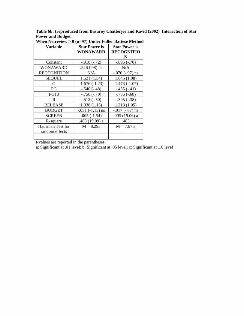
Table 6b: (reproduced from Basuroy Chatterjee and Ravid (2002) Interaction of Star Power and Budget When Netreview > 0 (n=97) Under Fuller Battese Method

Variable Star Power is WONAWARD

Star Power is RECOGNITIO

N Constant -.918 (-.72) -.896 (-.70)

WONAWARD .526 (.98) ns N/A RECOGNITION N/A -.070 (-.97) ns

SEQUEL 1.521 (1.54) 1.045 (1.08) G -1.676 (-1.23) -1.473 (-1.07)

PG -.540 (-.48) -.455 (-.41) PG13 -.756 (-.70) -.736 (-.68)

R -.512 (-.50) -.395 (-.38) RELEASE 1.338 (1.15) 1.218 (1.05) BUDGET -.031 (-1.15) ns -.017 (-.87) ns SCREEN .005 (-1.54) .005 (19.06) a R-square .483 (19.09) a .483

Hausman Test for random effects

M = 8.29a M = 7.67 a

t-values are reported in the parentheses a: Significant at .01 level; b: Significant at .05 level; c: Significant at .10 level