Are the World’s Poorest Being Left Behind?

Reconciling Conflicting Views on Poverty and Growth

Martin Ravallion1

Department of Economics, Georgetown University

Washington DC., 20057, U.S.A.

mr1185@georgetown.edu

Abstract: Traditional assessments of progress against poverty put no explicit

weight on increasing the standard of living of the poorest—raising the

consumption floor. Yet this is often emphasized by policy makers and moral

philosophers. To address this deficiency, the paper defines and measures the

expected value of the consumption floor as a weighted mean for the poorest

stratum. Using data for the developing world over 1981-2011, the estimated value

of the floor is about half the $1.25 a day poverty line. This is also very close to the

expected value of the national poverty line at the limit of zero consumption.

Economic growth has delivered only modest progress in raising the floor, despite

much progress in reducing the number living near the floor. This helps reconcile

the dramatic differences in prevailing views on poverty and growth.

Keywords: Poverty; growth; Rawls; development goals; safety-nets

JEL: I32, I38, O15

1 For helpful discussions on the topic of this paper and comments on the paper the author is grateful to Francois

Bourguignon, Mary Ann Bronson, Cait Brown, Shaohua Chen, Denis Cogneau, Garance Genicot, Peter Lanjouw,

Nkunde Mwase, Henry Richardson, Dominique van de Walle and seminar participants at the International Monetary

Fund.

2

1. Introduction

At the launch of the United Nations’ (2011) Millennium Goals Report, the U.N.’s

Secretary-General Ban Ki-moon said that:

“The poorest of the world are being left behind. We need to reach out and lift them into our

lifeboat.”

This view that the world’s poorest have been left behind is heard quite often. To give another

example, a press release by the International Food Policy Research Institute carried the headline:

“The world’s poorest people not being reached.”2

Yet other observers appear to tell a strikingly different story. They use aphorisms such as

“a rising tide lifts all boats” or they point to seemingly credible evidence that “growth is good for

the poor” or that the poor are “breaking through from the bottom.”3

This paper tries to make sense of these seemingly conflicting views on this important

question. The central issue is how we should assess progress against poverty. The approach of

economists and statisticians has been to count the poor in some way. One might track the

proportion of the population living below some deliberately low poverty line or use a more

sophisticated measure giving higher weight to poorer people. A prominent early advocate of this

approach was Arthur Bowley (the first Professor of Statistics at the London School of

Economics) who wrote 100 years ago that: 4

“There is perhaps no better test of the progress of a nation than that which shows what proportion

are in poverty; and for watching the progress the exact standard selected as critical is not of great

importance, if it is kept rigidly unchanged from time to time.” (Bowley, 1915, p.213.)

I dub this the counting approach. The theoretical foundations of the approach are found in a large

literature on poverty measurement, in which various axioms have been proposed.5

2 The press release was for an IFPRI report Ahmed et al. (2007).

3 The first expression is attributed to John F. Kennedy, the middle claim is the title of an influential paper by Dollar

and Kraay (2002), reiterated by Dollar et al. (2013), while the last expression is due to Radelet (2015). 4 There are antecedents in the literature. On the history of thought on measuring poverty see Ravallion (2015).

5 The most commonly used axioms are: (i) focus: that the measure of poverty should be unaffected by any changes

in the incomes (or consumptions) of those who are not deemed to be poor ; (ii) monotonicity: that, holding all else

constant, the measure of poverty must rise if a poor person experiences a drop in her income; (iii) subgroup

monotonicity: that aggregate poverty falls when any sub-group becomes poorer; (iv) scale invariance: that the

measure is unchanged when all incomes and the poverty line increase by the same proportion; (v) the transfer

principle: that the measure of poverty falls whenever a given sum of money is transferred from a poor person to

someone even poorer. An influential early contribution to the axiomatic foundations was made by Sen (1976),

although Sen’s proposed measure did not satisfy all of the above axioms. Other axioms have also been proposed; for

a fuller listing and further discussion see Foster et al. (2013).

3

This approach indicates falling incidence of absolute poverty in the developing world

over recent decades, when judged by poverty lines typical of developing countries.6 However,

Ban Ki-moon’s view could still be right if past applications of the counting approach have

missed the poorest. The poorest subset of the poor can be called the “ultra-poor.”7 In principle,

progress against poverty can be achieved in large part by lifting people near the poverty line out

of poverty, with little gain to the ultra-poor. That is not what this paper finds. Using various

definitions, the progress we have seen over the last 30 years in reducing the number of people

living under $1.25 a day has come with roughly similar progress in lifting people out of ultra-

poverty. By this approach many of the poorest have gained from rising overall affluence.

However, the paper argues that the counting approach does not adequately address

prevailing concerns about whether the poorest are left behind. Logically, for the poorest to not be

left behind in a period of overall economic growth there must be an increase in the lower bound

to the distribution of levels of living. That lower bound can be called the consumption floor,

which we can think of as the typical level of living of the poorest stratum. Human physiology

makes the existence of a positive floor plausible, given the nutritional requirements for basal

metabolism. This can be called the “the biological floor.” In practice, however, we would hope

that the actual consumption floor rises above the biological floor. Private social interactions can

probably provide some degree of protection. A consumption floor above the biological minimum

can also stem from a policy-supported minimum income.

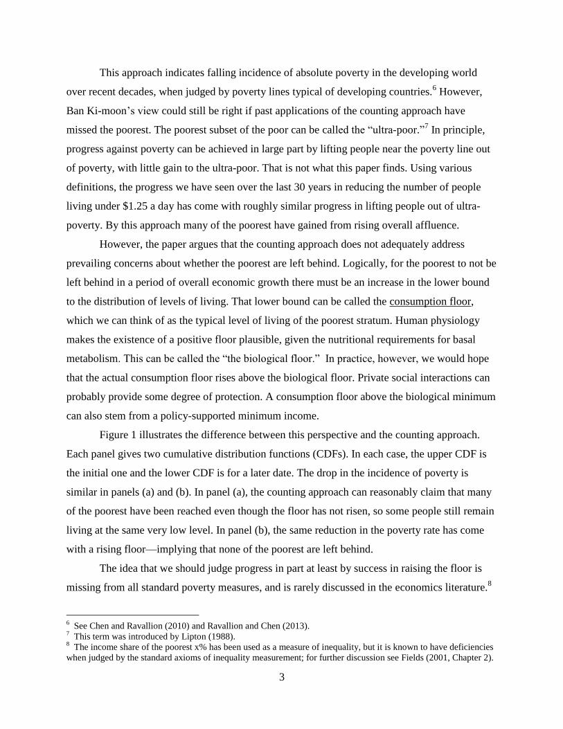
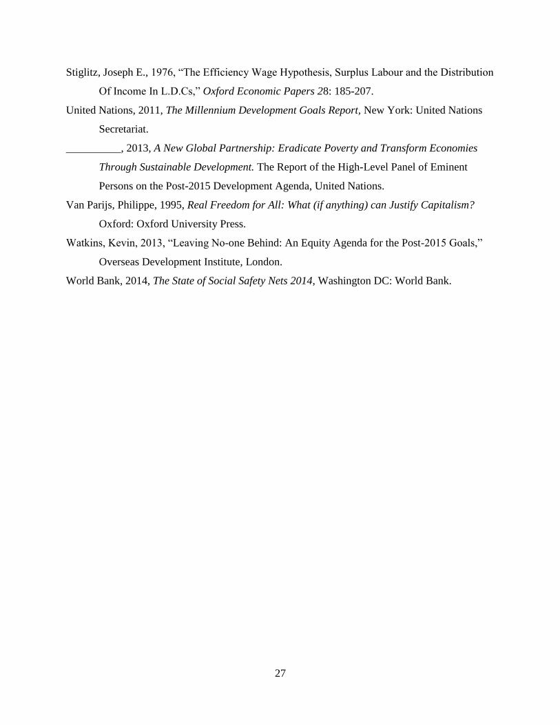
Figure 1 illustrates the difference between this perspective and the counting approach.

Each panel gives two cumulative distribution functions (CDFs). In each case, the upper CDF is

the initial one and the lower CDF is for a later date. The drop in the incidence of poverty is

similar in panels (a) and (b). In panel (a), the counting approach can reasonably claim that many

of the poorest have been reached even though the floor has not risen, so some people still remain

living at the same very low level. In panel (b), the same reduction in the poverty rate has come

with a rising floor—implying that none of the poorest are left behind.

The idea that we should judge progress in part at least by success in raising the floor is

missing from all standard poverty measures, and is rarely discussed in the economics literature.8

6 See Chen and Ravallion (2010) and Ravallion and Chen (2013).

7 This term was introduced by Lipton (1988).

8 The income share of the poorest x% has been used as a measure of inequality, but it is known to have deficiencies

when judged by the standard axioms of inequality measurement; for further discussion see Fields (2001, Chapter 2).

4

The concept of the consumption floor is conceptually distinct from existing poverty lines.9

Naturally, any poverty line aims to reflect what “poverty” means in a specific society, on the

understanding that (potentially many) people live below that level. The poverty line is a

normative concept, while the consumption floor is a positive one. Nor do standard poverty

measures necessarily reflect any progress in raising the floor. Although a higher consumption

floor (ceteris paribus) automatically reduces any measure of consumption poverty satisfying the

monotonicity axiom, none of the standard axioms of poverty measurement attach any explicit

weight to the level of the floor. This is due, at least in part, to the difficulties in identifying the

floor.10

Given the current interest in assuring that no one is left behind, this is surely a gap in the

current “dashboard” of development indicators.

Focusing on the floor can draw support from a literature, though largely outside

economics. An important school of moral philosophy has argued that we should judge a society’s

progress by its ability to enhance the welfare of the least advantaged, following the principles of

justice proposed by John Rawls (1971).11

By this view, a higher floor (as in Figure 1(b)) is not

only preferred, but is the main criterion of distributive justice (subject to other criteria of liberty,

as identified by Rawls).12

While Rawls’s “difference principle” is often interpreted as “maximin”

(to maximize the minimum level of welfare), Rawls insisted that some degree of averaging was

required in defining the “least advantaged”:

“I assume that it is possible to assign an expectation of well-being to representative individuals

holding these positions.” (Rawls, 1971, p. 56, my emphasis.)

I call the idea of focusing on the expected welfare of the poorest stratum in assessing social

progress the Rawlsian approach.

The difference between the two approaches illustrated by Figure 1 begs some questions

for which we currently have little idea of the answers: The consumption floor plausibly exists,

but at what level? What is the relationship between the two approaches? Has success judged by

9 For further discussion of poverty lines in theory and practice see Ravallion (2012).

10 See, for example, Freiman’s (2012) comments on Rawls’s difference principle.

11 Rawls proposed two principles of distributive justice. First, each person should have equal right to the most

extensive set of liberties compatible with the same rights for all. Second, subject to the constraint of liberty, social

choices should only permit inequality if it is efficient to do so—that a difference is only allowed if both parties are

better off as a result; this is what Rawls called the “difference principle.” 12

While popularity need not guide ethical judgments it is at least notable in the context of understanding debates

about distributive justice that there is experimental evidence indicating that a non-negligible number of people make

distributional judgments consistently with a Rawlsian “maximin” criterion (Michelbach et al., 2003).

5

the counting approach also come with success in raising the floor, such as through new social

protection policies in developing countries?

The task of addressing these questions calls for a method of estimating the level of the

consumption floor. When we refer to the “typical level of living of the poorest stratum” we are

acknowledging that consumption may be low at one date for purely transient reasons. Identifying

the floor as the strict lower bound of the distribution of consumption would be unsatisfactory as

this could well be subject to idiosyncratic transient factors, and possibly sizeable measurement

errors. We need an approach that is likely to be robust to transient effects and errors, but is still

operational with the data available.

The paper proposes an approach that can be implemented with readily available

secondary data sources. The method aims to identify an expected consumption floor amongst

those who are identified as poor in absolute terms by the standards of poor countries. Echoing

the above quote from Rawls (1971), the floor is an expectation formed over a stratum of people

with low observed consumption levels, where the expectation is weighted more heavily on the

poorest. Specifically, the lowest observed consumption is assumed to have the highest

probability of being at the floor, but that probability is less than one. The probability declines

linearly as consumption rises above the lowest observed value up to some critical point, above

which there is zero probability of being the poorest. Then the idea of the consumption floor can

be interpreted in terms of standard, readily available, poverty measures. The paper also compares

this to an alternative approach based on national poverty lines. The national line is interpreted as

the expected value of the consumption floor plus a relative component proportional to actual

mean consumption. Both methods indicate a consumption floor today that is about half of the

international poverty line of $1.25 a day.

The paper then shows that, while the counting approach shows huge progress for the

poorest, the Rawlsian approach does not. The distribution of the gains amongst the poor has

meant that the estimated consumption floor has risen little over those 30 years. While there has

been marked progress in reducing the numbers of the ultra-poor, and the poorest have not been

left behind, the expected value of the lowest level of living amongst those who are considered

poor by developing country standards has advanced rather little.

After reviewing the literature and policy discussions related to the idea of a consumption

floor (Section 2), the paper describes the data to be used in this study (Section 3). Then it turns to

6

the two proposed definitions of the floor and their empirical implementations (Sections 4 and 5).

Next the paper presents new evidence using the counting method (Section 6). Section 7 looks at

the empirical relationships with rates of growth in average living standards. Section 8 concludes.

2. The consumption floor in theory and policy

While the Rawlsian approach of using success in raising the consumption floor as an

indicator of social progress has not been favored by economists, it has deep roots in development

and social-policy thinking. Versions of the approach thrive today in policy discussions.

In a famous example, in 1948 (shortly before his assassination) Mahatma Gandhi was

asked “How can I know that the decisions I am making are the best I can make?” He answered:

“I will give you a talisman. Whenever you are in doubt, or when the self becomes too much with

you, apply the following test. Recall the face of the poorest and the weakest man whom you may

have seen, and ask yourself if the step you contemplate is going to be of any use to him. Will he

gain anything by it?” (Gandhi, 1958, p.65)

The spirit of Gandhi’s talisman was echoed (in somewhat dryer terms) 65 years later in a report

initiated by the U.N. on setting new development goals, which argued that:

“The indicators that track them should be disaggregated to ensure no one is left behind and targets

should only be considered ‘achieved’ if they are met for all relevant income and social groups.”

(United Nations, 2013, Executive Summary; my emphasis)

Endorsing this view, Kevin Watkins (2013, p.1) refers explicitly to Gandhi’s talisman, and

argues that “As a guide to international cooperation on development, that’s tough to top.”

If the poorest person sees a gain in permanent consumption then (by definition) the

consumption floor must rise. Social policies aim in part to support consumption levels at a point

well above the biological minimum. Indeed, something close to the Rawlsian approach and

Gandhi’s talisman has long been proposed as a guiding principle for thinking about antipoverty

policy in rich and poor countries alike. One motivation for the laws establishing statutory

minimum wage rates that first appeared in the late 19th

century is that they help raise the

consumption floor.13

From the 1970s, we started to see arguments in support of the idea of a

“basic-income guarantee”—a fixed cash transfer to every adult person.14

The idea is that the

13

There are also well-known efficiency arguments, notably in non-competitive labor markets. The first minimum

wage law was introduced by New Zealand in 1894. 14

This too is an old idea, with antecedents going back to at least Thomas Paine’s (1797) pamphlet Agrarian Justice

recommending the all agrarian land should be subject to taxation—a “ground rent,” the revenue from which should

be allocated equally to all adults in society, as all have a claim to that property.

7

basic income would provide a firm floor to living standards. This idea has gained momentum

since in the 1990s in both rich and poor countries.15

When financing through a progressive

income tax, the idea becomes formally similar to Milton Friedman’s (1962) Negative Income

Tax. The International Labor Organization (2012) has recommended a comprehensive “Social

Protection Floor,” comprising “nationally defined sets of basic social security guarantees”

spanning health, schooling and income security.

While economists measuring poverty have not attached any special significance to the

level of the consumption floor, the concept has long played a role in positive economics. Indeed,

the idea goes back to the first economists. Early ideas of the “subsistence wage” can be

interpreted as the wage rate required to assure that the biological floor is reached for a typical

family. The idea of a consumption floor played a key role in classical economics.16

Famously,

the Reverend Thomas Malthus (1806) argued that the economic dynamics of population growth

assures that the unskilled wage rate stays at the subsistence level; any temporary increase

(decrease) in the consumption of working-class families in a neighborhood of the floor would

induce population growth (contraction). The idea of a floor has been a feature of development

models for dualistic economies since Arthur Lewis’s (1954) model postulated a perfectly elastic

supply of labor to the developing modern sector at the subsistence wage.

The idea has continued to play a role in modern economics. It has been built into demand

models, such as the widely-used linear expenditure system. The idea is found in modern

theoretical treatments of the problem of determining the optimal population size.17

The idea of a

consumption floor is also found in modern dynamic models.18

For example, some theoretical

models have postulated an instantaneous utility function of the Stone–Geary form; consumers

then maximize the present value of the utility stream subject to their consumption not falling

below the floor (in addition to other standard constraints).19

There are also arguments on the

production side, whereby the existence of a floor generates a low-level non-convexity in

production possibility sets. Various theoretical arguments have been made to generate such non-

15

See, for example, Van Parijs (1995), Raventós (2007) and Bardhan (2011). 16

See Blaug’s (1962) discussion of the classical model of wage determination. 17

See Dasgupta (1993, Chapter 13). Blackorby and Donaldson (1984) proposed that social welfare increases with a

larger population if and only if the extra people have a level of consumption above a critical minimum. This can be

interpreted as an ethical floor, unlike the consumption floor, which is a positive concept. 18

See, for example, Azariadis (1996), Ben-David (1998) and Kraay and Raddatz (2007). 19

An example is found in Lopez and Servén (2009), who add a subsistence consumption parameter to the type of

model discussed in Aghion et al. (1999).

8

convexities. The essential argument is that worker productivity and/or access to credit (given

default likelihoods) suffer when a person’s consumption is close to the floor.20

Such arguments suggest an efficiency case for policy effort to raise the floor, in addition

to the equity case. In response to both efficiency and equity concerns, the new millennium has

seen a significant change in the set of development policies, which have come to embrace a

range of direct interventions, variously called “antipoverty programs,” “social safety nets,” and

“social assistance;” here I call them social safety nets (SSN’s).21

Their common feature is the use

of direct income transfers to poor families. This was rare in the developing world prior to the

mid-1990s, but today almost every country has at least one SSN program (World Bank, 2014).

The only estimate made to date (to my knowledge) indicates that 0.75-1 billion people in

developing countries currently receive social assistance (Barrientos, 2013). The new SSN

programs have mainly in the form of conditional cash transfers and workfare schemes (World

Bank, 2014). The compilation of survey-based estimates of SSN coverage spanning 2000-2010

in the World Bank’s ASPIRE database suggests that the proportion of the population receiving

help from SSN programs is growing rapidly, although there are probably selection biases in the

data.22

The term “safety net” evokes the idea of a floor, and some of the programs can be

interpreted as efforts to raise the floor, including the two largest programs to date in terms of

population coverage, namely China’s Di Bao program and India’s National Rural Employment

Guarantee Scheme, which is interpretable as an attempt to enforce the minimum wage rate in an

informal economy.23

Raising the consumption floor is a common motivation for SSN programs.

The fact that SSN coverage is expanding gives hope that the floor is rising. Of course,

whether this is happening in practice is another matter. Despite the expansion of SSN programs,

the majority of the poor are still not covered; the ASPIRE data indicate that only about one-third

20

Examples include Mirrlees (1975), Stiglitz (1976), Dasgupta and Ray (1986), Lipton (1988) and Banerjee and

Newman (1994). 21

A good working definition is: “Social safety nets are non-contributory transfers designed to provide regular and

predictable support to targeted poor and vulnerable people.” (World Bank, 2014, p.xii.) 22

Comparing the latest and earliest surveys for the 25 countries with more than one observation in the ASPIRE

database (with observations spanning 2000-2010) I find that the overall coverage rate (percentage of the population

as a whole receiving help from the SSN) is increasing at an average proportionate rate of 9.1% per annum (standard

error of 2.8%); in levels the rate is 3.5% points per year (standard error of 1.1% points). However, there may well be

selection bias in this sample, whereby the introduction of a SSN program stimulates survey data collection. 23

The Di Bao program makes transfers to bring urban residents up to locally determined “Di Bao lines” (see, for

example, Ravallion, 2014b). The Rural Employment Guarantee Scheme in India aims to guarantee up to 100 days of

work per household per year doing unskilled manual labor at stipulated minimum wage rates; see Dutta et al. (2014).

9

of the poorest quintile in the developing world receives any help from SSNs.24

To assess whether

economic growth and expanding SSN coverage is achieving progress against poverty

consistently with the Rawlsian approach, one needs to define and measure the consumption

floor. No such definition and measure is currently available.

Given the prominence of the idea of a consumption floor in moral philosophy and social

policy, as well as in positive economics, it is of interest to see how one might make the idea

operational—to quantify the expected level of the floor and how it has evolved over time,

including in response to economic growth. That is the task of the rest of the paper.

3. Data and descriptive statistics

The primary data source is the World Bank’s PovcalNet website. Here only a brief

summary is provided.25

The database draws on distributional data from 900 surveys spanning

125 developing countries. Using the most recent survey for each country, 2.1 million households

were interviewed. All poverty measures are estimated from the primary (unit record or tabulated)

sample survey data rather than relying on pre-existing estimates. Prior truncations of the data

(trimming the bottom or top) are avoided as far as possible, and appear to be rare at the bottom of

the distribution. Past estimates are updated to ensure internal consistency with new data.26

Households are ranked by either consumption or income per person, with consumption being

preferred when both are available. About 70% of the surveys allow a consumption-based

measure. The measures of consumption (or income, when consumption is unavailable) are

reasonably comprehensive, including both cash spending and imputed values for consumption

from own production. All distributions are weighted by household size and sample weights. The

poverty count is the number of people living in households with per capita consumption or

income below the international poverty line. All currency conversions are at purchasing power

parities using the results of the 2005 round of the International Comparison Program.27

The main

24

These are data for around 2008-2011. The one-third calculation uses the estimates in ASPIRE for October 2014

and is population-weighted. 25

The sources and estimation methods are described in greater detail in Chen and Ravallion (2010). 26

The version of the data set used here is for November 2014. 27

Adjusting this $1.25 line consistently with the new PPPs available 2011, the equivalent line in PPP $’s for India

(say) is about $2.00 a day in 2011 prices. (This is calculated by converting the $1.25 a day line for 2005 to Indian

rupees and then converting to 2011 local prices using the CPI for India, and converting back to 2011 $’s using the

2011 PPP.) This line gives a poverty measure for India very close to the measure using $1.25 a day at 2005 PPP.

10

international poverty line is $1.25 a day as proposed by Ravallion et al. (2009) who provide

various rationales for this line.

The surveys were mostly done by governmental statistics offices as part of their routine

operations. Not all available surveys are included in PovcalNet. A survey was dropped if there

were known to be serious comparability problems with the rest of the data set. Obvious problems

were addressed by either re-estimating the consumption/income aggregates or by dropping a

survey. Of course, there are data problems that cannot be dealt with, and differences in survey

methods can create differences in the estimates obtained.

The latest results from these data confirm past findings that the developing world has

seen impressive progress against absolute poverty over the last 30 years, with signs of

acceleration since 2000. The proportion of the developing world’s population living below $1.25

a day fell from 53% to 17% over this 30-year period.

4. Estimating the consumption floor as a weighted mean

With a sound sampling design and large enough representative samples we can be

confident about our estimate of the overall mean from a survey. But it is less clear how reliably

we can estimate the consumption floor—the lower bound of the distribution of consumption. If

we knew the true consumptions we could confidently estimate the floor directly from a

sufficiently large sample. However, there are measurement errors and transient consumption

shortfalls, whereby observed consumption in a survey falls temporarily below the floor (such as

due to illness), but recovers soon after the survey is done. How then might we estimate the floor?

The expected value of the consumption floor: The first method of estimating the floor

defines it as a weighted mean of the observed consumptions of the poorest stratum, with highest

weight on the poorest. A special case is the actual observed consumption of the poorest, with

zero weight on everyone else. This cannot, however, be treated as a reliable estimate of the

typical level of living of the poorest. For one thing, there will be transient effects on

consumption, such as due to shocks. There will also be measurement errors.28

More believably,

there is a positive probability that anyone within some stratum of undeniably poor people is in

fact the poorest, but that those who appear to be poorer are more likely to be closer to the true

28

Here measurement errors can be taken to include both statistical errors—reporting errors, selective non-

response—and mistakes in measurement, such as in calibrating price indices.

11

floor. In the spirit of Rawls’s formulation of distributive justice, we can thus justify forming a

pro-poor weighted expected value.

To formalize the approach, letminy denote the lowest level of permanent consumption in a

population. This is the consumption floor. We have an n-vector of observed consumptions, y.

The task is to use that data to estimate )( min yyE . As usual we can write:

n

i

ii yyyyE1

min )()( (1)

Here the probability that person i, with the observed iy , is in fact the worst off person is denoted

)Pr()( minyyy ii . The probabilities are not data, of course. But there are some seemingly

defensible assumptions we can make. The key assumption is as follows:

Assumption on the probability of being the poorest: Beyond some critical level *y of

consumptions in the survey data there is no chance of being the poorest person in terms

of latent permanent consumption. For those observed to be living below *y the

probability of observed consumption being the true lower bound of permanent

consumption falls monotonically as observed consumption rises until *y is reached.

This guarantees that the expected value of the floor cannot exceed the (un-weighted) mean of

observed consumptions for those living under *y , which is a logically defensible property. By

implication, the probability of being the poorest person is highest for the person who appears to

be worst off in the data. This also seems reasonable, but it is certainly not guaranteed to hold.

The assumption will fail if there is a sufficiently large under-estimation of consumption for the

lowest observed value in the data.

Intuitively, the extent of inequality amongst those living below *y must play a role in

determining the expected value of the floor. Imagine that all those living below *y have the same

observed consumption, the mean *y for the q persons with *yyi . Then it would be reasonable

to treat *y as the floor (assuming that the errors average out to zero). Now introduce inequality

amongst the poor. This implies a larger spread of y’s below the mean and hence a lower

)( min yyE relative to*y , given that the lower observed y’s are more likely to be near the floor.

12

Inequality amongst the poor is reflected in various distribution-sensitive poverty

measures, satisfying the standard transfer axiom in poverty measurement. The most widely-used

distribution-sensitive measure is the squared-poverty gap,

Zy

i

i

nzySPG /)/1( 2 where z is

the poverty line; this measure was introduced by Foster, Greer and Thorbecke (FGT) (1984). Let

*SPG denote the value of SPG when *yz . Intuitively, we expect a higher *SPG to be

associated with a lower expected floor for any given*y . The precise relationship between the

floor and measures of poverty also depends on the distribution of the errors in estimating the

lowest consumption level, to which we now turn.

To derive an operational measure, the assumption of monotonic-decreasing probabilities

is now specialized as:

)/1()( *yyky ii for *yyi (2)

0 for *yyi

To assure that the probabilities sum to unity we require that )/(1 *nPGk where

*

/)/1( **

yy

i

i

nyyPG is the poverty gap index for a poverty line of *y . Thus )( iy is person

i’s share of the aggregate poverty gap treating *y as the poverty line.

An operational formula for )( min yyE in terms of the FGT poverty measures can now be

derived. There are two steps. First, note that the expected value of the floor relative to *y is a

weighted mean of the values of the */ yyi (for *yyi ) with weights given by each person’s

share of the aggregate gap:

*

**min /)(/)(yy

ii

i

yyyyyyE (3)

Next, consider the value of ** / PGSPG . By construction, this is a weighted mean of the values

of */1 yyi conditional on *yyi , also with weights given by the shares of the poverty gap:

*

)/1)((/ ***

yy

ii

i

yyyPGSPG (4)

13

Comparing (3) and (4) we immediately have the following formula for the expected value of the

consumption floor (in $’s per person per day):

)/1()( ***min PGSPGyyyE (5)

It is plain that the poverty measures can suggest progress even when the expected value

of the floor is falling. For example, if y = (0.50, 0.50, 1.00, 1.25, 2.5, 5) and 25.1* y then

PG=0.233 and SPG=0.127; the expected value of the floor is 0.57. Suppose that the distribution

changes to (0.50, 0.50, 1.25, 1.25, 2.5, 5). Then both PG and SPG show an improvement (the

indices falling to 0.200 and 0.120 respectively) but the floor has fallen to 0.50.

It is plain from (4) that the necessary and sufficient condition for a rising floor is that the

proportionate rate of decline in PG exceeds that for SPG when using *y as the poverty line.

Intuitively, a rising floor requires faster progress against the distribution-sensitive poverty gap

measure, SPG, when based on the observed consumptions. If both poverty measures are falling

then one requires that SPG is falling faster than PG for the expected value of the floor to rise.

While the formula in (5) makes the relationship between the expected floor and poverty

measures clear, it is still not obvious what role is played by inequality amongst the poor. With

some straightforward algebra, the following alternative formula can be derived:29

**

2*

*min )(yy

yyyE

(6)

where

*

/)( 2*2*

yy

i

i

qyy is the sample variance amongst those for whom *yyi . This

makes clear how the gap between *y and )( min yyE reflects the inequality amongst those with

*yyi , as measured by their variance of consumption normalized by the mean gap, ** yy .

The formula in (5) can be generalized by setting )/1()( *yyky ii ( 1 ), giving:

)/1()( **

1

*

1 PPyyxE (7)

where:

29 This formula is derived by first noting that 2*2*2*2** /)/1()/(/)/1(

*

yyynqnyySPG i

yy

i

i

and

that )/1)(/( ** yynqPG i and then substituting into (5).

14

*

)/1(1 **

yy

i

i

yyn

P

(8)

This is the FGT class of measures for *yz . However, while the FGT measures naturally

emerge analytically, the interpretation of the parameter is different. Here determines how

the probability of being the poorest person falls as observed consumption increases, rather than

the degree of aversion to inequality amongst the poor, as in the FGT index.

Note that 0 can be ruled out; the probability must fall as consumption increases. To

put the point another way, if one uses 0 then every consumption below *y is equally likely to

be the lowest value, so )/1( 01

* PPy is the mean consumption of the poor (*y ). However, values

of 1 can be defended, to allow the probability to decline non-linearly. The choice of 1

(rather than 2 or higher) is made for a practical reason, namely that PovcalNet only gives values

of P for 2,1,0 .

Estimates of the consumption floor: One can take either an absolute or relative approach

to setting *y . The former approach sets *y at a constant value in real terms, while the latter fixes

instead the proportion of the population who could be living at the floor. However, it does not

seem plausible that the same proportion of the population could be living at the floor in a poor

society as a rich one; it is more believable that the poorer the society the larger the set of people

who could be living at the floor if we knew their true permanent consumption.

Using the absolute approach, a plausible assumption for *y is to set it according to

poverty lines found in the poorest countries. This is one of the methods used by Ravallion et al.

(2009) to set the international poverty line of $1.25 a day. So the first key assumption made here

for implementing the approach outlined in theory above is that there is no chance that any

observed consumption level above $1.25 a day corresponds to a true level of consumption that is

in fact the floor. The $1.25 line corresponds closely to the 20th

percentile in 2010. So this is quite

a wide range. I test sensitivity to using a lower value for *y of $1.00 a day and using a relative

definition, such that a constant percentage of the population is identified as the group of people

who may be living at the true floor.

Table 1 gives my estimates of the expected value of the floor from the data described in

Section 2. The table gives the estimated floor for z=$1.00 as well as $1.25, although the

15

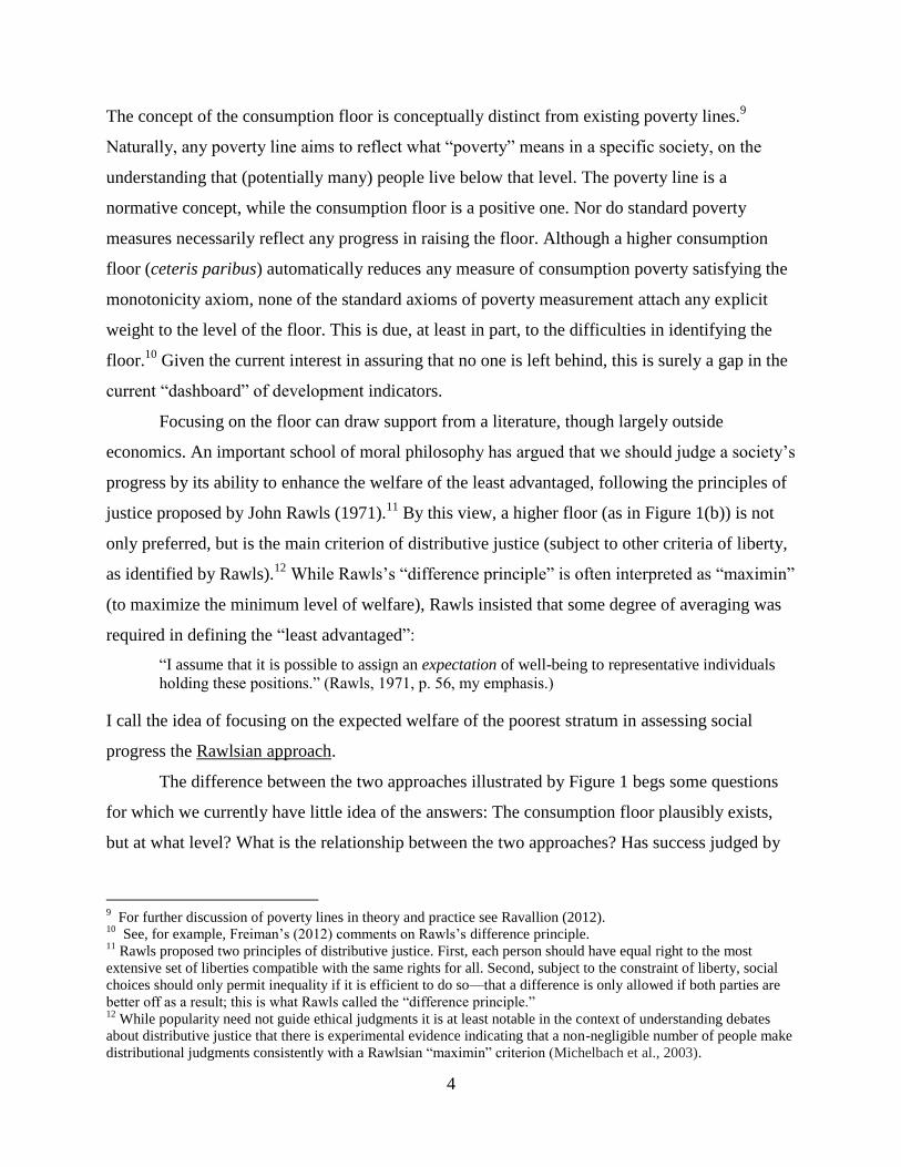
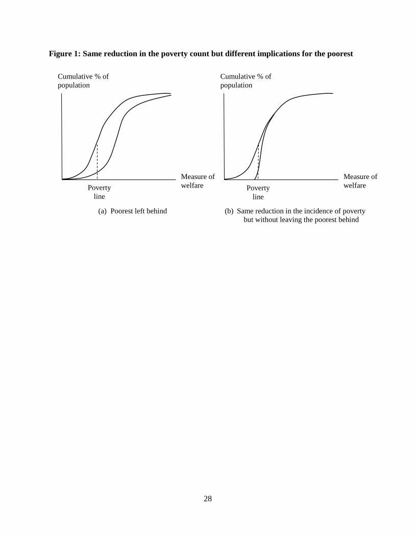
discussion will focus on the latter case. Figure 2 plots the estimated consumption floor over

1981-2011, as well as the mean consumptions of both the poor and the overall population of the

developing world. Panel (b) gives a “blow-up” of the lower portion, also identifying the

contribution of inequality amongst the poor, i.e., )/( **2* yy (recalling equation (5)).

The estimate of the expected value of the lowest consumption level is $0.67 per day.30

The main source of statistical imprecision in this estimate is the cut-off point*y . The global

sample sizes for estimating *SPG and

*PG are huge (over 2 million sampled households from

over 900 surveys for the recent years, though less as one goes back in time). Using the Ravallion

et al. (2009) estimate of the standard error of the $1.25 a day poverty line, the implied standard

error of the present estimate of the floor is $0.10 per day.31

The 95% confidence interval for the

consumption floor is thus $0.47 to $0.87 per day.

It should be recalled that this assumes that there is zero probability of an observed

consumption above $1.25 a day corresponding to the floor. Naturally, a higher (lower) *y will

raise (lower) the estimated floor. If anything, I suspect that $1.25 is on the high side.

Alternatively, if one sets *y =$1.00 then the time mean of the floor falls to $0.55.32

Also notice that this estimation method does not of course require that nobody should be

found living below the expected consumption floor. That would be too stringent. Even putting

measurement errors aside, at any one survey date there will invariably be some people

temporarily living below any consumption floor. For 2011, PovcalNet indicates that 3.7% of the

population of the developing world lived below $0.67 a day. The proportion living below the

lower bound of the 95% confidence interval for this estimate of the floor is 1.8%.33

It is evident from Figure 2 that the estimated floor has proved to be quite stable over

time; indeed, the inter-temporal standard error is less than $0.01 per day (although this does not

30

This is the un-weighted mean over time. The inter-temporal variance is so low that it is unlikely that population

weighting would make any detectable difference. 31

Ravallion et al. (2009) used Hansen’s (2002) estimator for a piece-wise linear (“threshold”) model in estimating

the standard error of the lower (flat) segment of the relationship between national poverty lines and private

consumption per person. 32

For an upper bound on *y one might assume instead that nobody above the median consumption for the

developing world could be living at the floor. This would entail *y =$2.00 per day (for 2005), in which case the

time-mean of the estimated floor rises to $0.90 a day. However, the median is an implausibly high value of for z. 33

This is probably an overestimate given that PovcalNet uses grouped data for many countries, which require curve

fitting; the software uses parameterized Lorenz curves fitted to the grouped data. These will give non-zero estimates

to very low levels, even when the micro data do not indicate any observations.

16

factor in all the sources of variance as reflected in the “full” standard error of $0.10). The

estimated consumption floor rose by only 9 cents per day over 30 years, from $0.59 to $0.68,

reflecting a (slightly) steeper pace of decline in *SPG and

*PG . The contribution of inequality

amongst those living below $1.25 rose from $0.14 to $0.20 over the period (Table 1, Column 5),

representing 19% and 23% of *y respectively.

The growth rate in the floor (regression coefficient of )(ˆln min yyE on time) is 0.34% per

annum, with a standard error of 0.08%. There is divergence between the mean for the poor as a

whole and the estimated floor, with a growth rate for the former of 0.46% per annum (s.e.=0.06).

(And the divergence is statistically significant; t-test=4.39; prob.=0.14%.) Using an upper bound

of $1.00 a day there is even less sign of a positive trend in the implied floor; the estimate of the

floor rises from $0.52 to $0.53 over the period, although it rises then falls (Table 1).34

However, the divergence between the mean for the poor and the expected consumption

floor is minor compared to the expanding gap between both and the overall mean of household

consumption per person (Figure 2), which grew at an annual (per capita) rate of 2.1% over this

period (s.e.=0.24%) and the rate of growth roughly doubled from the turn of the century.

Strikingly, there is no sign that the upsurge in average living standards in the developing world

since 2000 has put upward pressure on the consumption floor (Figure 7). In relative terms, the

consumption floor has fallen from 22% of the mean in 1981 to 13% in 2011.

The above results have used a fixed absolute standard for setting *y (either $1.25 or $1.00

a day). It was argued that this is more plausible than a relative approach to defining the stratum

of people who could be living at the floor. However, it should be noted that using a relative

standard implies a rising absolute floor over time. For example, suppose one focuses instead on

the poorest 20%, corresponding closely to the absolute standard of $1.25 a day in 2010. If one

defines the group of people who are potentially living at the floor in 1981 as the poorest 20%

then the estimate of )( min yyE falls to $0.37 a day, with a value of *y for that year of $0.63

(only slightly higher than the estimate of )( min yyE using *y =$1.25). This suggests far greater

progress in raising the floor than the absolute approach, with its value almost doubling over 30

years. The “relative floor” has remained a fairly constant % of the overall mean (14% in 1981

34

The trend coefficient is very close to zero (a coefficient of 0.0002, with a standard error of 0.0009).

17

and 13% in 2011). The bulk of the drop in the floor for 1981 using the relative definition for *y

is due to the fact that the relative bound has almost halved; the value of SPG/PG is not much

different between the two approaches (0.53 in 1981 using the absolute approach versus 0.42

using the relative approach).

5. The consumption floor implicit in national poverty lines

A national poverty line can be thought of as the sum of two components: an absolute

consumption floor plus a relative component that depends positively on the country’s mean

consumption. This suggests an alternative method of defining the floor as the expected value of

the national poverty line at zero mean. How does this compare to the method in Section 3?

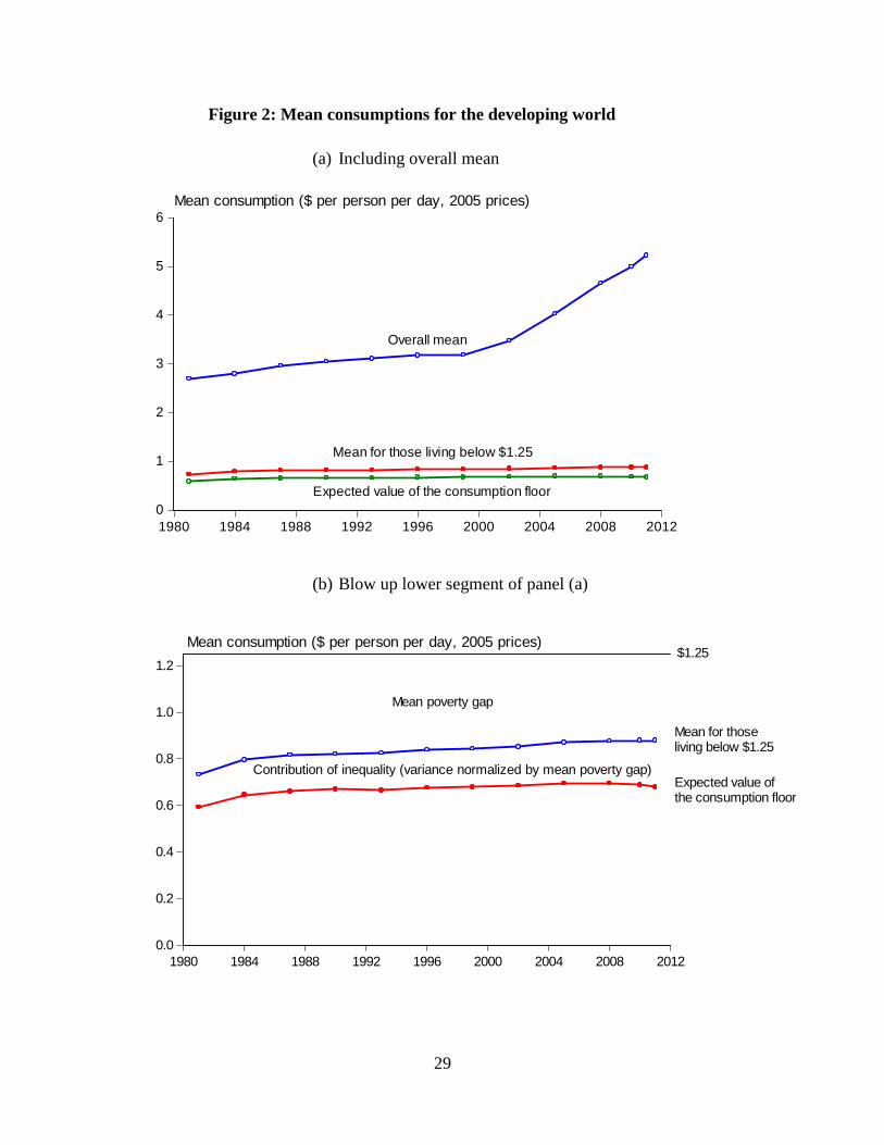
Figure 3 plots national poverty lines for developing countries. Regressing the national

line (z) on the mean ( y ) from the closest available household survey one obtains for country i:35

iii yz ̂530.0647.0)064.0()288.0(

R2=0.709, n=73 (9)

The implied consumption floor of $0.65 per day is not significantly different from the prior

estimate of $0.67 in Section 3, based on very different data.36

This level of agreement can be

interpreted as largely independent support for the assumption that *y =$1.25 in the first method

of estimating the consumption floor.

The national lines were set at different dates. On adding a time trend to the above

regression one finds no significant drift in the consumption floor.37

However, with only one

observation of the poverty line per country this can only be considered a weak test. The results in

Table 1 are clearly more convincing on this point.

Another implication of (9) is notable. Given that the floor is found to be positive, the

national lines are weakly relative, as defined by Ravallion and Chen (2011). By implication,

when all incomes rise by a fixed proportion, the poverty rate falls, as distinct from the strongly

relative lines set at a constant proportion of the mean or median, as used in Western Europe.38

35

White standard errors in parentheses. I also tested an augmented model with a cubic function of the mean, but the

higher-order terms were individually and jointly insignificant. 36

The mean national line at the lowest national consumption is $1.22 a day. 37

The coefficient on the year in which the poverty line was set is 0.0008 (s.e.=0.0005). 38

Eurostat (2005) uses such relative poverty measures as does the Luxembourg Income Study (LIS).

18

6. Revisiting the counting approach

As discussed in the introduction, the traditional counting approach suggests that the gains

to the poor of the developing world over the last 30 years have reached many of the poorest. This

section re-examines that approach in the light of the findings above.

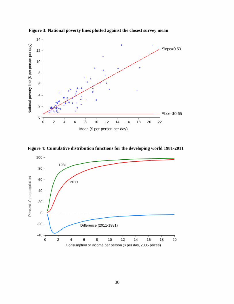
Figure 4 gives the cumulative distribution functions (CDF’s) for 1981 and 2011.39

We see

that there is first-order dominance, implying an unambiguous reduction in poverty for all

possible lines and all additive measures, as was found by Chen and Ravallion (2010) for a

shorter period.40

There is a feature of Figure 4 that immediately suggests that there has been little

gain in the level of the floor (although this point has not been made before to my knowledge).

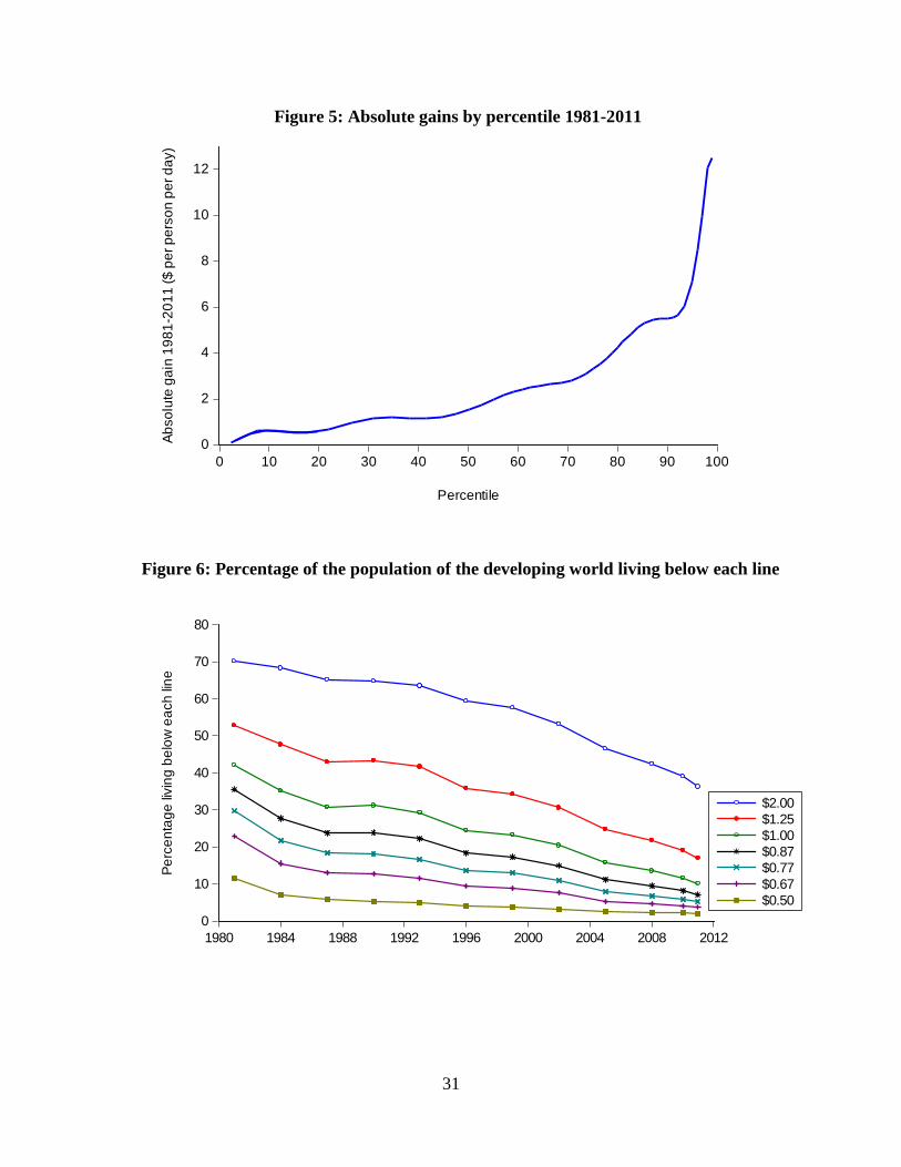
Figure 5 makes this clearer by giving the monetary gain at each percentile implied by Figure 4,

i.e., the absolute difference between the quantile functions, obtained by inverting the CDFs.41

(These gains are simply the horizontal differences between the CDFs in Figure 4.) Consistently

with the lack of progress in raising the floor we see that the gains are close to zero for the

poorest, but rising to quite high levels. This is also consistent with what we know about rising

absolute inequality in the developing world (Ravallion, 2014).

A further insight from Figure 5 is that there are larger absolute gains for the second decile

from the bottom (though fairly flat between the 10th

and 20th

percentiles). Using the 20th

percentile as the cut-off point in the relative approach is thus picking up these gains. At a

sufficiently low cut-off, even the relative approach will show little gain in the floor.

Might the counting approach pick up the lack of progress for the poorest if one looks well

below the $1.25 line? To provide a simple measure of the incidence of ultra-poverty using the

counting approach, it is defined here as the share of the population living below $0.87 a day.

This is the upper bound of the 95% confidence interval for the estimated consumption floor in

the developing world, as described in Section 4. The use of the 95% confidence interval is

essentially arbitrary. I also give the main results for a line of $0.77 a day, one standard error

above the point estimate, and for a measure of poverty that gives higher weight to those living

39

The CDF is truncated above $20 a day to give greater detail at the lower end; however, there is dominance all the

way to the top. 40

On the implications of first-order dominance in this context see Atkinson (1987). 41

The empirical quantile function is used for 1981. For the purpose of creating the graph, the quantile function for

2011 was based on a 10th

degree polynomial, which fitted extremely well (R2=0.998), although the top 2% were

trimmed from the GIC as these are considered less reliable.

19

closer to the floor. However, it should not be forgotten that the claim that poverty has fallen is

robust to the poverty line (Figure 4).

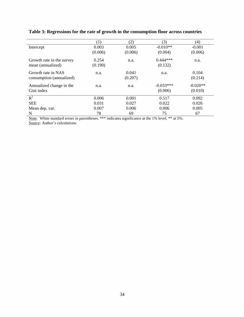
In the earliest survey rounds in PovcalNet, the incidence of ultra-poverty by the $0.87

line varies across countries from zero to 89%. It has declined steadily over time in the

developing world as a whole (Figure 6) and for most countries; see Figure 7, comparing the

earliest and latest surveys for those countries in PovcalNet with two or more surveys. In the

latest surveys the proportion varies from zero to 75%. The number of people living in ultra-

poverty fell from 1,317 (35.4%) million to 423 million (7.1%) over this period. (Using the more

stringent definition of $0.77 a day, the percentage declined from 1,098 million (29.6%) to 308

million (5.2%) in 2011.) For the developing world as a whole, the share of total poverty

represented by the ultra-poor fell from 67% in 1981 to 42% in 2011.

The bulk of the reduction in overall poverty rates (for $1.25 a day or $2.00) is

accountable to a lower incidence of ultra-poverty. Between 1981 and 2011 the $1.25 a day

poverty rate fell by 35.8% points; almost 80% of this decline (28.4% points) is accountable to the

decline in the ultra-poverty rate.

The trend (regression coefficient on time) over 1981-2011 for the percentage of ultra-

poor is -0.83% points per annum (with a standard error of 0.07%).42

This is lower than the trend

for the percentage below $1.25 a day of -1.13% (s.e.=0.04%), but the difference is not large, with

the implication that the bulk of the inter-temporal variance in the overall poverty rate is

accountable to progress against ultra-poverty; the R2 for the regression of the overall poverty rate

for $1.25 and the ultra-poverty rate for $0.87 is 0.97. Even more strikingly, progress against

ultra-poverty also accounts for the bulk of the progress against poverty judged by the $2.00 line.

The poverty rate for the latter line has an annual trend of -1.12% (s.e.=0.09%), almost identical

to that for the $1.25 line. For the $2.00 line, the R2 for the regression of the overall poverty rate

on the ultra-poverty rate for $0.87 is 0.91.

This pattern is also evident at country level. Over three-quarters (77.4%) of the variance

in annualized rates of poverty reduction using the $1.25 line is accountable to rates of progress

against ultra-poverty. Only 13.6% is accountable to changes in the density of those who were

poor but not ultra-poor; the covariance term accounts for 9.0%. Figure 8 plots the rate of change

in P0 for $1.25 a day across countries against the corresponding change in the ultra-poverty rate.

42

For the $0.77 line the annual trend is -0.69% (s.e.=0.05).

20

There is close to a 1-to-1 relationship; as the number of ultra-poor in a country falls, we also see

roughly similar exit rates from the ranks of the poor population as a whole.

This pattern is suggestive of a process of what can be called rank-preserving lifting out of

poverty. It is as though, as one of the group of “poor but not ultra-poor” is lifted out of poverty

this frees up space for one of the ultra-poor, who moves up to take that spot on the ladder. But

the floor rose very little.

7. Growth and the poorest

In the light of these findings, let us now revisit the longstanding debate about how much

poor people have benefited from economic growth.43

A stylized fact that has emerged from the

literature on developing countries is that growth in average living standards tends to come with

lower incidence of absolute poverty.44

Typically this has been demonstrated by focusing on

prevailing poverty lines for low income countries, such as represented by the $1.25 a day line.

However, the incidence of ultra-poverty is no less responsive to growth in the mean. This

is demonstrated in Table 2, which gives the “least-squares elasticity”—the regression coefficient

of the annualized proportionate rates of poverty reduction between the earliest and latest survey

rounds on the corresponding growth rates in the mean.45

Results are given for three estimators of

the growth rate in the mean: that based on the same surveys, the growth rate of private

consumption from the national accounts (NAS), and the simple mean of these. There are

arguments one can make for and against each estimator. The survey mean has the advantage that

it is automatically for exactly the same time as the survey used to measure poverty, while the

NAS consumption is annual (for the year in which the survey was done). However, there is a

concern that measurement errors may bias the estimate based on the survey mean growth rates; if

the growth rate in the survey mean is over-estimated then the reduction in the poverty rate will

also tend to be underestimated. (The direction of total bias is theoretically ambiguous given that

there is also the usual attenuation bias due to measurement error in a regressor.) Private

consumption in the NAS for developing countries is typically calculated as a residual at the

43

Ravallion (2015) provides an overview of this debate. 44

See Ravallion (1995, 2001) and Dollar and Kraay (2002). Ferreira and Ravallion (2009) review the literature. 45

More precisely, this is the regression coefficient of iitit iPP /)/ln( (where itP is the poverty measure for

country i at date t and i is the time interval since the previous survey) on iitit iMM /)/ln( (where itM is the

mean for country i at date t).

21

commodity level (after deducting other measured sources of domestic absorption) rather than

being calibrated to surveys. Different price indices are also typically relevant to the two series,

although a correlation between the errors in the price indices cannot be ruled out. So the

problem of correlated measurement errors is less severe using NAS growth rates, but it does not

vanish. The third estimate simply splits the difference between the two growth rates.

The main lesson from Table 2 is that it cannot be claimed that the growth elasticities are

lower (in absolute value) for the ultra-poor. Indeed, the NAS growth rates suggest even higher

elasticities for the ultra-poverty poverty rates.

By contrast, the consumption floor using the absolute approach has responded little to

economic growth. The least-squares elasticity of the country-specific consumption floors to the

survey mean is 0.254, with a standard error of 0.190 (n=78); the elasticity is not significantly

different from zero at the 10% level. Using instead the growth rates based on NAS consumption,

the least-squares elasticity is even lower at 0.041 (s.e.=0.207; n=69). As can be seen from Table

3, a significant relationship with the growth rate in the survey mean emerges when one controls

for the change in overall inequality as measured by the annualized change in the Gini index.

However, this is not robust to using the NAS growth rate instead (comparing columns 3 and 4 of

Table 4). Rising inequality remains a robust covariate of changes in the floor.

8. Conclusions

A clue to understanding why we hear very different answers to the question posed in the

title of this paper can be found in the conceptual difference between focusing on counts of poor

people (following in the footsteps of Bowley and others) versus focusing on the level of living of

the poorest, in the spirit of Gandhi’s talisman or the Rawlsian difference principle. Both

perspectives are evident in past thinking and policy discussions. Both have been advocated as

development goals, although the counting approach, as implemented in various poverty

measures, has long monopolized the attention of economists and statisticians monitoring

progress against poverty.

The paper has demonstrated that our success in assuring that no-one is left behind can be

readily monitored from existing data sources under certain assumptions. The proposed approach

recognizes that there are both measurement errors and transient consumption effects in the

observed data. However, the data are assumed to be reliable enough to assure that it is more

22

likely that the person with the lower observed consumption is living at the floor than anyone

else. To make this approach operational with available data, the paper has made some

simplifying assumptions that might be relaxed in future work. The empirical measure used here

assumes that the probability of any observed consumption being the floor falls linearly up to an

assumed upper bound. Then the ratio of the squared poverty gap to the poverty gap relative to

that bound—two readily-available poverty measures—emerges as the key (inverse) indicator for

assessing progress in raising the floor.

Drawing on the results from household surveys for developing countries spanning 1981-

2011, the paper finds considerable progress against poverty using the counting approach. There

is first-order dominance over the 30 years, implying an unambiguous reduction in absolute

poverty by the counting approach over all lines and all additive measures (including distribution-

sensitive measures). Standard poverty measures have responded to economic growth, and that

holds for lines well below $1.25 a day (corresponding to the poorest 20% in 2010). Indeed, the

bulk of either the inter-temporal or the cross-country variance in rates of poverty reduction for

either $1.25 or $2.00 a day is accountable to progress for those living under $0.87 or even $0.77

a day. Elasticities of poverty incidence to economic growth are no lower for lower lines.

However, there appears to have been very little absolute gain for the poorest. Using an

absolute approach to identifying the floor, the increase in the level of the floor seen over the last

30 years or so has been small—far less than the growth in mean consumption. The modest rise in

the mean consumption of the poor has come with rising inequality (specifically, a rising variance

normalized by the mean poverty gap), leaving room for only a small gain in the level of living of

the poorest. The bulk of the developing world’s progress against poverty has been in reducing

the number of people living close to the consumption floor, rather than raising the level of that

floor. Growth in mean consumption has been far more effective in reducing the incidence of

poverty than raising the consumption floor. In this sense, it can be said that the poorest have

indeed been left behind.

Stronger indications of a rising floor are found if one adopts a relative approach to

defining the upper bound on consumption for those people who could conceivably be living at

the floor, and one sets the fixed percentage at a sufficiently high level. For example, focusing on

the poorest 20% suggests considerable progress in raising the expected value of the floor.

However, the paper has argued that an absolute approach makes more sense on the grounds that

23

one expects a poorer society to have more people living near the floor, as is found to be the case

empirically using the counting approach.

To anticipate one response, it might be argued that progress in lifting the floor is a

second-order issue, as long as fewer people live near the floor. That is implicit in the traditional

counting methods used to assess progress against poverty. However, proponents of this view

must surely take pause when one notes that for a long time, and across countries at very different

levels of development, social policies have often claimed that they aim to ensure a minimum

level of living above any biological consumption floor required for mere survival. Negative

income tax schemes and (formally-equivalent) basic-income guarantees financed by progressive

income taxes aim to raise society’s consumption floor above the biological minimum. And such

efforts are not confined to rich countries; indeed, the two largest anti-poverty programs in the

world today (in China and India) aim to raise the floor. In forming their views, casual observers

may well focus on the observed level of living of those they deem to be the poorest. The level of

the floor is salient to understanding the continuing debates about poverty and growth.

While it would be ill-advised to look solely at the level of the floor, it can be

acknowledged that this has normative significance independently of attainments in reducing the

numbers of people living near that floor. The thesis of this paper is not that progress against

poverty should be judged solely by the level of the consumption floor, but only that the latter

should no longer be ignored.

24

References

Aghion, Philippe, Eve Caroli and Cecilia Garcia-Penalosa, 1999, “Inequality and Economic

Growth: The Perspectives of the New Growth Theories,” Journal of Economic Literature

37(4): 1615-1660.

Ahmed, Akhter, Ruth Vargas Hill, Lisa C. Smith, Doris M. Wiesmann, and Tim Frankenberger,

2007, The World’s Most Deprived. Washington DC: International Food Policy Research

Institute.

Atkinson, Anthony B., 1987, “On the Measurement of Poverty,” Econometrica 55: 749-764.

Azariadis, Costas, 1996, “The Economics of Poverty Traps: Part One. Complete Markets,”

Journal of Economic Growth 1: 449–496.

Banerjee, Abhijit, and Andrew Newman, 1994, “Poverty, Incentives and Development,”

American Economic Review 84(2): 211-215.

Bardhan, Pranab, 2011, “Challenges for a Minimum Social Democracy in India,” Economic and

Political Weekly 46(10): 39-43.

Barrientos, Armando, 2013, Social Assistance in Developing Countries. Cambridge: Cambridge

University Press.

Ben-David, Dan, 1998, Convergence Clubs and Subsistence Economies, Journal of Development

Economics 55: 153–159.

Blackorby, Charles, and David Donaldson, 1984, “Social Criteria for Evaluating Population

Change,” Journal of Public Economics 25: 13–33.

Blaug, Mark, 1962, Economic Theory in Retrospect, London: Heinemann Books.

Bowley, Arthur L., 1915, The Nature and Purpose of the Measurement of Social Phenomena.

London: P.S. King and Sons.

Chen, Shaohua, and Martin Ravallion, 2010, “The Developing World is Poorer than we Thought,

but no Less Successful in the Fight against Poverty,” Quarterly Journal of Economics

125(4): 1577-1625.

Dasgupta, Partha, 1993, An Inquiry into Well-Being and Destitution, Oxford: Oxford University

Press.

Dasgupta, Partha, and Debraj Ray, 1986, “Inequality as a Determinant of Malnutrition and

Unemployment,” Economic Journal 96: 1011-34.

25

Dollar, David, and Kraay, Aart, 2002, “Growth is Good for the Poor,” Journal of Economic

Growth 7(3): 195-225.

Dollar, David, Tatjana Kleineberg and Aart Kraay, 2013, “Growth Still is Good for the Poor,”

Policy Research Working Paper 6568, World Bank.

Dutta, Puja, Rinku Murgai, Martin Ravallion and Dominique van de Walle, 2014, Right-to-

Work? Assessing India’s Employment Guarantee Scheme in Bihar. World Bank.

Eurostat, 2005, “ Income Poverty and Social Exclusion in the EU25,” Statistics in Focus 03

2005, Office of Official Publications of the European Communities, Luxembourg.

Fields, Gary, 2001, Distribution and Development, New York: Russell Sage Foundation.

Freiman, Christopher, 2012, “Why Poverty Matters Most: Towards A Humanitarian Theory Of

Social Justice,” Utilitas 24(1): 26-40.

Friedman, Milton, 1962, Capital and Freedom. Chicago: University of Chicago Press.

Foster, James, J. Greer, and Erik Thorbecke, 1984, “A Class of Decomposable Poverty

Measures,” Econometrica 52: 761-765.

Foster, James, Suman Seth, Michael Lokshin, and Zurab Sajaia, 2013, A Unified Approach to

Measuring Poverty and Inequality. Washington DC: World Bank.

Gandhi, Mahatma, 1958, The Last Phase, Volume II. Ahmedabad: Navajivan Publishing House.

Hansen, Bruce E., 2000, “Sample Splitting and Threshold Estimation,” Econometrica 68:

575-603.

International Labor Organization, 2012, “R202:Social Protection Floors Recommendation,”

Recommendation concerning National Floors of Social Protection Adoption, Geneva,

101st ILC session (14 June 2012).

Kraay, Aart, and Claudio Raddatz, 2007, “Poverty Traps, Aid and Growth,” Journal of

Development Economics 82(2): 315-347.

Lewis, Arthur, 1954, “Economic Development with Unlimited Supplies of Labor,” Manchester

School of Economic and Social Studies 22: 139-191.

Lipton, Michael, 1988, “The Poor and the Ultra-Poor: Some Interim Findings,” Discussion Paper

25, World Bank, Washington DC.

26

Lopez, Humberto, and Luis Servén, 2009, “Too Poor to Grow,” Policy Research Working Paper

5012, World Bank.

Malthus, Thomas Robert, 1806, An Essay on the Principle of Population, 1890 Edition, London:

Ward, Lock and Co.

Mirrlees, James, 1975, “A Pure Theory of Underdeveloped Economies,” in: L. G. Reynolds

(ed.), Agriculture in Development Theory, New Haven: Yale University Press.

Michelbach, Philip A., John T. Scott, Richard E. Matland, and Brian H. Bornstein, 2003, “Doing

Rawls Justice: An Experimental Study of Income Distribution Norms,” American

Journal of Political Science 47(3): 523–539.

Paine, Thomas, 1797, Agrarian Justice, 2004 edition published with Common Sense by Penguin.

Radelet, Steven, 2015, The Great Surge: The Unprecedented Economic and Political

Transformation of Developing Countries Around the World. Simon & Schuster.

Ravallion, Martin, 1995, “Growth and Poverty: Evidence for Developing Countries in the

1980s,” Economics Letters 48, 411-417.

__________, 2001, “Growth, Inequality and Poverty: Looking Beyond Averages.” World

Development 29(11): 1803-1815.

__________, 2012, “Why Don’t we See Poverty Convergence?” American Economic Review

102(1): 504-523.

__________, 2014, “Income Inequality in the Developing World,” Science 344: 851-5.

__________, 2015, The Economics of Poverty, New York and Oxford: Oxford University Press.

Ravallion, Martin, and Shaohua Chen, 2011, “Weakly Relative Poverty,” Review of Economics

and Statistics 93(4): 1251-1261.

__________, 2013, “More Relatively Poor People in a Less Absolutely Poor World,” Review of

Income and Wealth 59(1): 1-28.

Ravallion, Martin, Shaohua Chen and Prem Sangraula, 2009, “Dollar a Day Revisited,” World

Bank Economic Review 23(2):163-184.

Raventós, Daniel, 2007, Basic Income: The Material Conditions of Freedom, London: Pluto

Press.

Rawls, John, 1971, A Theory of Justice, Cambridge MA: Harvard University Press.

Sen, Amartya, 1976, “Poverty: An Ordinal Approach to Measurement,” Econometrica 46: 437-

446.

27

Stiglitz, Joseph E., 1976, “The Efficiency Wage Hypothesis, Surplus Labour and the Distribution

Of Income In L.D.Cs,” Oxford Economic Papers 28: 185-207.

United Nations, 2011, The Millennium Development Goals Report, New York: United Nations

Secretariat.

__________, 2013, A New Global Partnership: Eradicate Poverty and Transform Economies

Through Sustainable Development. The Report of the High-Level Panel of Eminent

Persons on the Post-2015 Development Agenda, United Nations.

Van Parijs, Philippe, 1995, Real Freedom for All: What (if anything) can Justify Capitalism?

Oxford: Oxford University Press.

Watkins, Kevin, 2013, “Leaving No-one Behind: An Equity Agenda for the Post-2015 Goals,”

Overseas Development Institute, London.

World Bank, 2014, The State of Social Safety Nets 2014, Washington DC: World Bank.

28

Figure 1: Same reduction in the poverty count but different implications for the poorest

(a) Poorest left behind (b) Same reduction in the incidence of poverty

but without leaving the poorest behind

Measure of

welfare

Cumulative % of

population

Measure of

welfare

Cumulative % of

population

Poverty

line

Poverty

line

29

Figure 2: Mean consumptions for the developing world

(a) Including overall mean

(b) Blow up lower segment of panel (a)

0

1

2

3

4

5

6

1980 1984 1988 1992 1996 2000 2004 2008 2012

Mean consumption ($ per person per day, 2005 prices)

Expected value of the consumption floor

Mean for those living below $1.25

Overall mean

0.0

0.2

0.4

0.6

0.8

1.0

1.2

1980 1984 1988 1992 1996 2000 2004 2008 2012

Mean consumption ($ per person per day, 2005 prices)

Mean for thoseliving below $1.25

Expected value ofthe consumption floor

Contribution of inequality (variance normalized by mean poverty gap)

$1.25

Mean poverty gap

30

Figure 3: National poverty lines plotted against the closest survey mean

Figure 4: Cumulative distribution functions for the developing world 1981-2011

0

2

4

6

8

10

12

14

0 2 4 6 8 10 12 14 16 18 20 22

Mean ($ per person per day)

Na

tio

na

l p

ove

rty lin

e ($

pe

r p

ers

on

pe

r d

ay)

Slope=0.53

Floor=$0.65

-40

-20

0

20

40

60

80

100

0 2 4 6 8 10 12 14 16 18 20

Pe

rce

nt o

f th

e p

op

ula

tio

n

Consumption or income per person ($ per day, 2005 prices)

1981

2011

Difference (2011-1981)

31

Figure 5: Absolute gains by percentile 1981-2011

Figure 6: Percentage of the population of the developing world living below each line

0

2

4

6

8

10

12

0 10 20 30 40 50 60 70 80 90 100

Percentile

Ab

so

lute

ga

in 1

98

1-2

01

1 ($

pe

r p

ers

on

pe

r d

ay)

0

10

20

30

40

50

60

70

80

1980 1984 1988 1992 1996 2000 2004 2008 2012

$2.00

$1.25

$1.00

$0.87

$0.77

$0.67

$0.50

Pe

rce

nta

ge

livin

g b

elo

w e

ach

lin

e

32

Figure 7: Changes in the incidence of ultra-poverty at country level

Figure 8: Progress against ultra-poverty at country level translated into progress against

total poverty

0

10

20

30

40

50

60

70

80

90

0 10 20 30 40 50 60 70 80 90

Ultra-poverty rate for the earliest survey (%)

Ultra

-po

ve

rty r

ate

fo

r la

test su

rve

y (

%)

Latest=earliest

-7

-6

-5

-4

-3

-2

-1

0

1

2

-7 -6 -5 -4 -3 -2 -1 0 1 2

Annualized % point change in the ultra-poverty rate

An

nu

alize

d %

po

int ch

an

ge

in

th

e to

tal p

ove

rty r

ate Slope=1.058

(s.e.=0.058)

33

Table 1: Estimated consumption floors the developing world

(1) (2) (3) (4) (5)

Estimated consumption floor Means Contribution of

inequality (variance

normalized by the

mean gap)

*y =$1.25 *y =$1.00 Mean

consumption

Mean

consumption of

those living below

$1.25 a day

1981 0.59 0.52 2.70 0.73 0.14

1984 0.64 0.56 2.80 0.80 0.15

1987 0.66 0.56 2.97 0.82 0.16

1990 0.67 0.57 3.05 0.82 0.15

1993 0.66 0.56 3.11 0.83 0.16

1996 0.68 0.56 3.18 0.84 0.16

1999 0.68 0.57 3.19 0.84 0.16

2002 0.68 0.57 3.48 0.85 0.17

2005 0.69 0.56 4.03 0.87 0.18

2008 0.69 0.56 4.66 0.88 0.18

2010 0.69 0.54 5.00 0.88 0.19

2011 0.68 0.53 5.23 0.88 0.20

Notes: All numbers are $ per person per day in 2005 prices using purchasing power parity rates for private

consumption. Source: Author’s calculations. Columns (1) and (2) use the estimates of PG and SPG from PovcalNet

and equation (4).

Table 2: Growth elasticities of poverty reduction for various poverty lines

Poverty line Growth rate based

on survey mean

Growth rate based

on NAS

consumption

Average of survey

mean and NAS

growth rates

$2.00 -1.681

(0.433; 98)

-1.494

(0.427; 87)

-1.817

(0.333; 87)

$1.25 -2.345

(0.628; 91)

-1.961

(0.494; 80)

-2.588

(0.402; 80)

$0.87 -2.072

(0.841: 77)

-2.332

(0.541; 68)

-3.247

(0.481; 68)

$0.77 -2.115

(0.881; 76)

-2.549

(0.565; 67)

-3.480

(0.520; 67)

Note: White standard errors in parentheses, followed by the number of observations.

All coefficients are significantly different from zero at the 1% level.

Source: Author’s calculations.

34

Table 3: Regressions for the rate of growth in the consumption floor across countries

(1) (2) (3) (4)

Intercept 0.003

(0.006)

0.005

(0.006)

-0.010**

(0.004)

-0.001

(0.006)

Growth rate in the survey

mean (annualized)

0.254

(0.190)

n.a. 0.444***

(0.132)

n.a.

Growth rate in NAS

consumption (annualized)

n.a. 0.041

(0.207)

n.a. 0.104

(0.214)

Annualized change in the

Gini index

n.a. n.a. -0.033***

(0.006)

-0.020**

(0.010)

R2 0.006 0.001 0.517 0.092

SEE 0.031 0.027 0.022 0.026

Mean dep. var. 0.007 0.006 0.006 0.005

N 78 69 75 67 Note: White standard errors in parentheses. *** indicates significance at the 1% level; ** at 5%.

Source: Author’s calculations.