1

Are Rural Areas Underserved by HUD’s Subsidy Programs?

Paul E. McNamara

Department of Agricultural and Consumer Economics,

University of Illinois at Urbana-Champaign

Email: mcnamar1@illinois.edu

Han Bum Lee

Department of Agricultural and Consumer Economics,

University of Illinois at Urbana-Champaign

Email: lee466@illinois.edu

Selected Paper prepared for presentation at the 2016 Agricultural & Applied Economics

Association Annual Meeting, Boston, Massachusetts, July 31-August 2

Copyright 2016 by McNamara and Lee. All rights reserved. Readers may make verbatim copies

of this document for non-commercial purposes by any means, provided that this copyright notice

appears on all such copies.

2

Are Rural Areas Underserved by HUD’s Subsidy

Programs?

Paul E. McNamara, University of Illinois at Urbana-Champaign

Han Bum Lee, University of Illinois at Urbana-Champaign

Abstract

Despite the extensive research exploring the effects of public provision of subsidized housing

opportunities in urban areas, especially large cities, in the United States, very little or no research

exists concerning the geographical inequality of federally funded rental subsidy programs in rural

areas. This paper uses a multilevel modelling approach to analyze the extent rural-urban spatial

disproportionality exist in rental subsidy programs of the U.S. Department of Housing and Urban

Development (HUD) across all counties in the 48 contiguous states. Results indicate that rural

residents in poverty are less likely to receive the rental subsidies by approximately 3.4 – 7.1

percentage points, based on different rural-urban geographical classifications and model

specifications, than those in urban areas. Also, the predicted estimates of heterogeneous state

effects reveal intergovernmental relationship of particularly how a state is involved in local

government’s administration of the rental subsidy programs.

Keywords: Rural poverty; HUD rental subsidy programs; Geographical inequality

3

Introduction

A federally funded rental subsidy program, managed by the U.S. Department of Housing and

Urban Development (HUD) in the United States, primarily provides housing subsidies to the

elderly, persons with disabilities, and low-income families who face a probable risk, in the absence

of the subsidy, of falling into poverty. In recent years, HUD has served approximately 5 million

eligible low-income families each year, devoting around $40 billion annually, which is over two-

thirds of federal spending on the Earned Income Tax Credit (EITC) and twice what is spent on the

Temporary Assistance for Needy Families (TANF) (Falk, 2012). Because of its national scale of

regulatory intervention and governance, and the large federal contribution, an extensive research

literature exists concerning the effectiveness of the federal rental subsidy program in assisting

vulnerable people and reducing spatial poverty concentration, as well as helping people move

toward employment and breaking the poverty cycle (i.e. Wilson, 1987; Currie & Yelowitz, 2000;

Katz, Kling, & Liebman, 2001; Goetz, 2003; Jacob, 2004; Jacob & Ludwig, 2012). However, the

majority of research efforts have concentrated on understanding the effects of public provision of

subsidized housing opportunities in urban areas, especially large cities under the urban antipoverty

political agenda, and very little research exists concerning the spatial inequality of federal rental

subsidy programs across rural and urban areas.

The research question we explore in this paper is does a rural-urban bias exist in the current

HUD rental subsidy programs across all counties in the 48 contiguous states? Also, given the

existence of the rural-urban effect, we examine the role of state government of particularly how

heterogeneous state characteristics are associated with the local government’s administration of

the rental subsidy programs. This paper adopts a multilevel modelling approach to explain

variation in the percent of people in poverty who received HUD’s rental subsidy programs (or

recipient-poor ratio), attributed by rural-urban geographic basis, in different geographic levels.

We structure a two-level model with counties (local governments or public housing authorities) at

the lower level grouped within the states at the higher level, enabling us to investigate how the

recipient-poor ratio varies at each level compared to the others, and at the same time to identify

plausible factors that may explain this variation. The main data set used in this paper is the HUD’s

2013 Picture of Subsidized Households (PSH) merged with the 5-year (2009-2013) American

Community Survey (ACS) data at the county level. Also, we adopt two rural-urban geographical

4

classifications using the Economic Research Service’s (ERS) 2013 Rural-Urban Continuum Codes

and HUD’s definition of rurality.

The remainder of the paper proceeds as follow: it begins by describing poverty in a rural

context and addressing its critical needs of the adequate rental subsidy programs. Then the paper

discusses the background information of the federally funded rental subsidy programs. The next

section presents data on the geographical distribution of the rental subsidy programs and the

comparison of selected rural-urban characteristics based on defined rural-urban geographical

classifications. The following section details the empirical strategy, discusses the regression results,

and performs robustness checks of the results. Lastly, the paper closes with concluding remarks.

Poverty in Rural America

Rural America has long suffered a disproportionate share of the nation’s poverty population

(Tickamyer & Duncan, 1990; Albrecht & Albrecht, 2000; Duncan & Coles, 2000). According to

the 2014 Census, 14.8 percent of the U.S. population (or 46.7 million persons) was poor (DeNavas-

Walt, 2014). Particularly, poverty is more prevalent among women, racial and ethnic minority

groups, people with low-socioeconomic status, and single-parent families. Because these

phenomenon are often presented as the nation’s urban problems, most of us tend to think of poverty

as being associated with metropolitan areas; however, in reality, nearly 16.5 percent of non-

metropolitan residents, which were 2 percentage points higher than those of metropolitan areas,

were impoverished. Also, the recent report from the ERS shows that persistent poverty existed in

301 counties in non-metropolitan areas, compared to 52 counties in metropolitan areas (Farrigan,

2015).1

Furthermore, severity and persistence of poverty in rural areas are often linked to a limited

opportunity structure – mainly derived from past social and economic development policies

targeting economic areas with promising higher returns, particularly in large urban centers, and

the industrialization of agriculture – associated with insufficient and unstable jobs (significant

decrease in share of agricultural employment), challenges in geographic and income mobility, and

1 The study defines persistent poverty as at least higher than 20 percent poverty rates in each U.S. Census 1980,

1990, 2000, and ACS 5-year estimates 2007-2011.

5

limited access to proper health care and decent affordable housing, as well as narrow investment

for community development and diversity in economic and other social institutions (Albrecht,

1998; Brown & Swanson, 2003; Conger & Elder, 1994; Duncan & Coles, 2000; Irwin et al., 2010;

Ricketts, 1999). Moreover, according to the 2014 National Rural Housing Coalition (NRHC)

report, nearly half (48 percent) of all rural renters are cost-burdened (spending 30 percent or more

of their monthly income), and about half of theses households pay more than 50 percent of their

monthly income toward housing. Without access to adequate rental subsidies, these people have

very few options for decent affordable housing, rendering them vulnerable toward homeless.

The Provision of Federally Funded Rental Subsidy Programs

HUD’s rental subsidy programs can be broadly divided into three major programs – public housing

(publicly owned housing), Section 8 Housing Choice Voucher (HCV) (privately owned housing),

and Section 8 Project-Based Voucher (PBV) programs (privately owned, subsidized housing).

Eligibility for HUD’s rental subsidy programs is limited to physically and financially

disadvantaged people, determined by applicants’ demographic status (elderly or disability status)

and annual gross income adjusted by family size.

Public housing was the first federal housing subsidy program, established by the Housing

Act of 1937, aimed at clearing slum-dwelling poor, especially in large cities, to create a better

living environment believed to improve their economic mobility (Hoffman, 1996, 2012). Rents for

the public housing tenants are limited to 30 percent of income, with public housing authorities

receiving federal operating subsidies intended to cover the difference between rental income and

operating costs. By 1950, the government had begun or completed construction of about 150,000

public housing units nationally. Through the next two decades of rapid expansion, the stock of

public housing units peaked at 1.4 million in 1991 (Schwartz, 2014). However, as the public

housing program grew, emerging issues (i.e. obsolete building conditions, inefficient utility costs,

racial and economic segregation) led to a policy shift to the tenant-based rental subsidy programs,

gradually diminishing the stock of public housing (Jencks & Mayer, 1990; Massey & Kanaiaupuni,

1993; Wilson, 1987).

6

Since the mid-1970s, the Section 8 HCV program has received greater attention as an

alternative public housing policy to resolve pre-existing problems, particularly the issue of low-

income minorities’ poverty concentration around public housing developments (i.e. Devine, Gray,

Rubin, & Taghavi, 2003; Newman & Schnare, 1997; Goering, Stebbings, & Siewert, 1995; Pendall,

2000; Lens, Ellen, & O’Regan, 2011; Turner, 1998). In contrast to the downward trend of public

housing units, the HCV program has grown to represent the nation’s largest housing subsidy

program, serving more than 2.2 million low-income families in conjunction with over 3,000 local

public housing authorities. Uniquely, the HCV program allows recipients the opportunity to rent

privately owned housing in any neighborhood within the jurisdiction of the local public housing

authority, allowing recipients more flexibility about where to live. Section 8 housing voucher

holders are generally obliged to pay the Total Tenant Payment (TTP) which is 30 percent of their

monthly income towards housing; however, the HCV program exceptionally allows an additional

10 percent of their income in situations where the gross rent exceeds the locally designated

payment standard representing the maximum allowable rent subsidy. HUD pays the subsidy to the

landlord of the unit selected by the tenant, provided the unit meets certain quality standards.

The Section 8 PBV program, which emerged in the 1960s, relies on a public-private

partnership in which federal government enters into contracts with private owners to provide

affordable housing for a specified number of years, after which the housing is converted to market

rate by owners’ decisions. Specifically, unlike the HCV program renewing the rental contract

every year, the PBV program provides owners with a guaranteed rental contract (a long-term

contract of 10 years) as long as the property remains in the assisted program. Recently, the PBV

program serves nearly 1.3 million low-income families, mostly elderly or disabled head of

households; however, this stock of housing is in danger of being permanently lost as a result of

owners opting out or physical deterioration of a property (Newman, 2005; Rice, 2009). Therefore,

a key challenge for this housing program is to incentivize existing owners to remain under contract,

as well as increase new owners’ program participation, to maintain the stock of affordable housing

for low-income families.

7

Data Set

The data set used in this paper is HUD’s 2013 Picture of Subsidized Households (PSH) merged

with the 5-year (2009-2013) American Community Survey (ACS) data at the county level.

Specifically, the PSH provides a total number of HUD’s rental subsidies including public housing,

Section 8 HCV, Section 8 PBV, Section 8 New Construction/Substantial Rehabilitation, Section

236, and Multi-family rental subsidy programs. Also, the 5-year ACS data set provides more

reliable estimates of demographic and socioeconomic characteristics at smaller geographic

boundaries than one-year and three-year estimates (Census Bureau, 2008). We use the 5-year ACS

data to obtain the number of households with income below the poverty threshold to calculate the

percent of poor who receive HUD’s rental subsidy programs. Additionally, other county-level and

state-level variables are obtained from the 5-year ACS data and 2013 Annual Survey of State

Government Finances.

We consolidate the data to the county level because HUD’s rental subsidy programs are

administered by local PHAs, distributed across more than 3,000 counties in the 48 contiguous

states of the United States.2 For the purpose of this analysis, we adopt HUD’s rural geographic

definition – a county with a population of 20,000 inhabitants or less, and not located in a

Metropolitan Statistical Area. According to HUD’s rurality definition, there are 1,464 rural

counties and 1,645 urban counties. Also, in order to confirm the robustness of the results, we

replicate the analysis with a different definition of rurality using the ERS’s 2013 Rural-Urban

Continuum Codes defining a county as rural if it belongs to the category “Completely rural or less

than 2,500 urban population.” According to the ERS geographical classification, there are 3,106

counties that include 626 counties in non-metropolitan rural areas and 2,480 counties in

metropolitan and non-metropolitan urban areas. Since the PSH contains observations that list

number of rental subsidies with no geographic identifier for each state, we exclude a total of 6,060

housing subsidies – 5,860 housing subsidies in New York State (about one percent of all allocated

housing subsidies), and 200 housing subsidies for the rest of the 47 states.3

2 Some PHAs manage public provision of the rental subsidy programs in city area rather than county (i.e. Chicago

Housing Authority, Housing Authority of Baltimore City, etc.). In order to run county-level analysis, we incorporate

city-based PHAs into county-based housing authority. 3 New York State consists of 62 counties with 49 urban counties (or 79%). Excluding 5,860 rental subsidies in

New York State may decrease the recipients-poor ratio of a certain county. For example, if majority of the rental

8

Regional Characteristics and Descriptive Statistics

Since the late 1970s, state and local governments have had an increasingly important role than

federal government in implementing programs and providing services more closely attuned to the

needs of specific communities and populations. In order to capture distinct effects of the

components determining the recipients-poor ratio at different geographical levels, we construct

the state- and county-level variables.

County-level variables: we measure poverty rates by dividing the number of persons with

income below the poverty threshold by the total number of persons in the county, and the

recipients-poor ratio represents the percent of persons in poverty who received HUD’s rental

subsidies. Rural is binary variable – 1 for rural and 0 for urban counties. Sex ratio indicates the

number of males per 100 females (divided by 100); elderly dependency ratio is the number of

persons 65 and older to every 100 persons of traditional working ages (divided by 100);

population-housing ratio represents the average number of persons in a housing unit; and

population density represents the average number of people living in a unit of an area (mile). Also,

percent black population, percent Hispanic population, percent disabled population; percent

single-parent family, median income, and median rent are included as county-level control

variables to increase precision of the estimates in the regression.

State-level variables: we measure public welfare expenditure by dividing state’s public

welfare expenditures (Medicaid, Supplementary Security Income (SSI), and TANF; and other

welfare services) by the number of persons in poverty in the state.4 Also, we include the state’s

intergovernmental expenditures since rural communities depend heavily on such transfers from

the states to provide local services (Felix & Henderson, 2010). Intergovernmental expenditure is

measured by the total amounts paid to local governments – “as fiscal aid in the form of shared

subsidies were missing from rural counties, it will decrease the recipients-poor ratio in rural counties which result in

upward bias of the rural effect estimate because this will create a greater gap of the recipients-poor ratio between rural

and urban counties. On the other hand, if majority were missing from urban counties, it will decrease the recipients-

poor ratio in urban areas resulting in a downward bias of the rural effect estimate. We first regress with all observed

counties, and then regress without New York state observations in order to see how the estimates (sign, statistical

significance, and the magnitude) change. 4 See State Government Finances glossary, Census Bureau, for detailed metric of public welfare expenditures.

9

revenues and grants-in-aid, as reimbursements for performance of general government activities

and for specific services for the paying government, or in lieu of taxes” (State Government

Finances, n.d.) – divided by the number of counties within the state. This represents the average

amount of the state’s transfers to each local government if all conditions are identical; however, in

reality, it is more likely that a larger share of transfers happens in metropolitan areas and large

cities potentially due to high population density (high demand for local services) and economic

returns. The state-level variables do not necessarily indicate the exact amount transferred to the

local governments, but they explain the specific state effect related to those expenditures on the

recipients-poor ratio in the regression, and the story of the rural effect conditioned on such

expenditures can be explained by the interactions with those variables with the rural variable.

These state-level variables are designed to capture state efforts – financial supports and means-

tested assistance programs dedicated to poverty alleviation and administration of general activities

and programs related, but not limited to, housing and community development on specific places

and populations in need – on the provision of HUD’s rental subsidy programs at the local

government level.

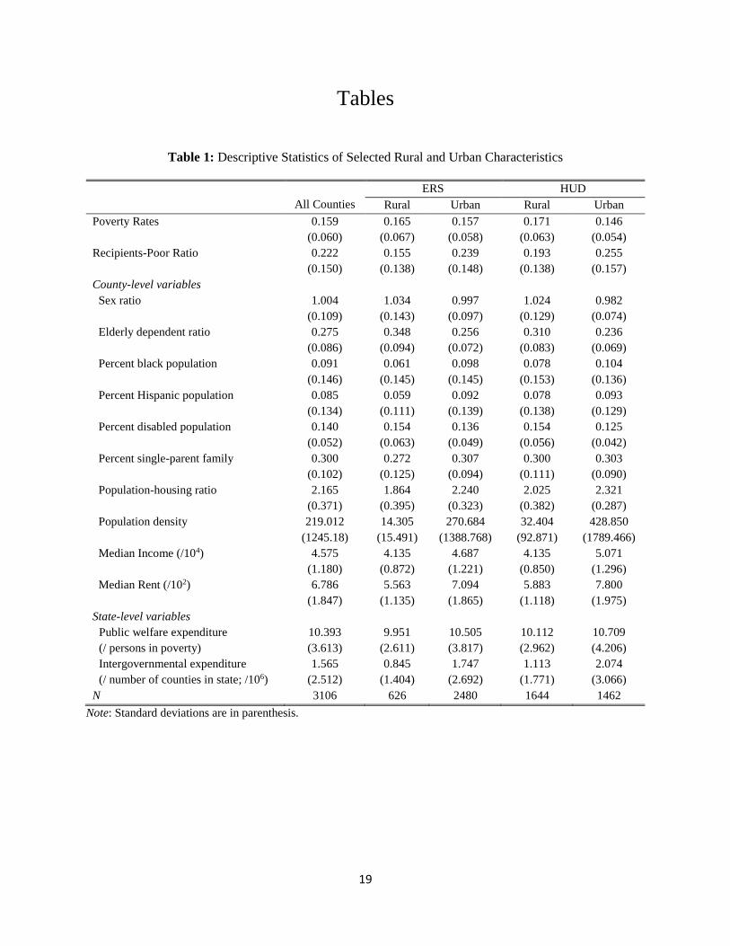
For more detailed comparison between rural and urban counties across the 48 contiguous

states, Table 1 presents descriptive statistics for the selected rural and urban characteristics. We

observe that overall poverty rates are shown to be higher in rural counties, and the gap of mean

poverty rates between rural and urban counties becomes greater using HUD’s rurality definition,

while, on average, the recipients-poor ratio in rural counties tends to be smaller than those in urban

counties (the absolute mean difference of the recipients-poor ratio is greater with the ERS

definition). Taken at face value, the results suggest that, although rural counties have higher

percentages of people living in poverty than the metropolitan/non-metropolitan urban counties,

HUD’s underprovides rental subsidy programs in rural counties. Also, rural counties tend to have

a higher level of sex ratio, elderly dependent ratio, proportion of disabled people, and population

density than those in urban counties; while, on average, rural counties tend to have a lower

proportion of minorities (black and Hispanic population) and single-parent families. Rural counties

have a lower level of population-housing ratio, median income, and median rent, and the results

show a distinct difference between rural and urban counties in population density and population-

housing ratio variables. Moreover, we observe that, on average, rural counties tend to be in states

10

with a relatively lower level of public welfare (adjusted by the number of persons in poverty) and

intergovernmental expenditures (adjusted by the number of counties in the state) than more

urbanized states.

Empirical Model

The multilevel models, also referred to as linear random coefficient model and hierarchical model,

have long been applied in the social sciences. The distinct feature of the model is to capture

regional random effects (heterogeneous state effects), and it also accounts for the correlation

between counties nested within the same state (non-independently identically distributed).

Additionally, the multilevel models address potential issues of spatial heterogeneity, assuming that

the effect of an explanatory variable can be different in each geographical level. For instance, in

some states, rural counties may be more strongly associated with the outcome variable than others,

indicating that the slope would vary from one state to another. In this paper, we structure a two-

level model in which county-level variables explain county (lower level) variation within a state,

and state-specific variables explain state (higher level) variance between states. If we denote by

𝑦𝑖𝑗 the outcome variable at the county, i, in state j (i = 1,… 𝑛𝑗; j = 1,…, J), the following equations

show a simple two level linear model:

𝑦𝑖𝑗 = 𝛽0𝑗 + 𝛽1𝑗𝑅𝑖𝑗 + 𝛽2𝑗𝑋𝑖𝑗 + 𝜀𝑖𝑗 (1)

𝛽0𝑗 = 𝛾00 + 𝛾01𝐶𝑗 + 𝑢0𝑗 . (2)

In Eq. (1), the outcome variable, 𝑦𝑖𝑗, can be modeled as a function of the mean outcome

variable for state j (𝛽0𝑗), rural-urban binary variable (𝑅𝑖𝑗), county-level control variables (𝑋𝑖𝑗), and

county-level errors (𝜀𝑖𝑗) that assume to be independent and normally distributed with a mean of 0

and a variance of 𝜎𝑒2 within each state. In Eq. (2), the state mean of the outcome variable (𝛽0𝑗), is

modeled as a function of a state-mean outcome variable (𝛾00), state-level variable (𝐶𝑗), and state-

level errors (𝑢0𝑗) which are assumed to be normally distributed with mean 0 and variance of 𝜎𝑢02 .

Specifically, 𝑢0𝑗 measures a state-specific deviation from the state-mean outcome (𝛾00) after

accounting for the effect of state-specific variable (𝐶𝑗). Variance of the residual errors of 𝜀𝑖𝑗 is

specified as 𝜎𝑒2. Substituting Eq. (2) into Eq. (1) yields the two level multilevel model shown as:

11

𝑌𝑖𝑗 = 𝛾00 + 𝛽1𝑗𝑅𝑖𝑗 + 𝛽2𝑗𝑋𝑖𝑗 + 𝛾01𝐶𝑗 + 𝑢0𝑗 + 𝜀𝑖𝑗 . (3)

Relaxing the assumption of the fixed coefficient in the Eq. (3) yields the random slope

model, in which, of particular relevance to our paper, we allow rural-urban binary variable (𝑅𝑖𝑗)

to vary randomly across states, shown as the following equation:

𝛽1𝑗 = 𝛾10 + 𝛾11𝐶𝑗 + 𝑢1𝑗, (4)

In Eq. (4), 𝛽1𝑗 (the regression coefficient of the effect of 𝑅𝑖𝑗 on 𝑌𝑖𝑗) can be modeled as

mean slope (𝛾10), state-specific variable (𝐶𝑗), and state-level errors (𝑢1𝑗) which represent the

deviation of the slope within each state from the overall slope 𝛾10 after accounting for the effect

of 𝐶𝑗. Substituting Eq. (4) into Eq. (3) yields the two level random slope model shown as:

𝑌𝑖𝑗 = 𝛾00 + 𝛾10𝑅𝑖𝑗 + 𝛽2𝑗𝑋𝑖𝑗 + 𝛾01𝐶𝑗 + 𝛾11𝐶𝑗 𝑅𝑖𝑗 + 𝑢1𝑗𝑅𝑖𝑗 + 𝑢0𝑗 + 𝜀𝑖𝑗. (5)

The state-level errors 𝑢0𝑗 and 𝑢1𝑗 are assumed to have a multivariate normal distribution

with expectation 0, and to be independent from the county-level residual errors (𝜀𝑖𝑗). The variance

of the residual errors 𝑢1𝑗 is specified as 𝜎𝑢02 . Also, covariance between 𝑢0𝑗 and 𝑢1𝑗 denote by 𝜎𝑢2

2

(for example, if is positive, as the intercept increases the slope increases). Eq. (5) includes the fixed

coefficients for county-level variables, state-level variables, and interaction terms, as well as it has

complex error structure including random intercept component and a random slope and individual

level errors.

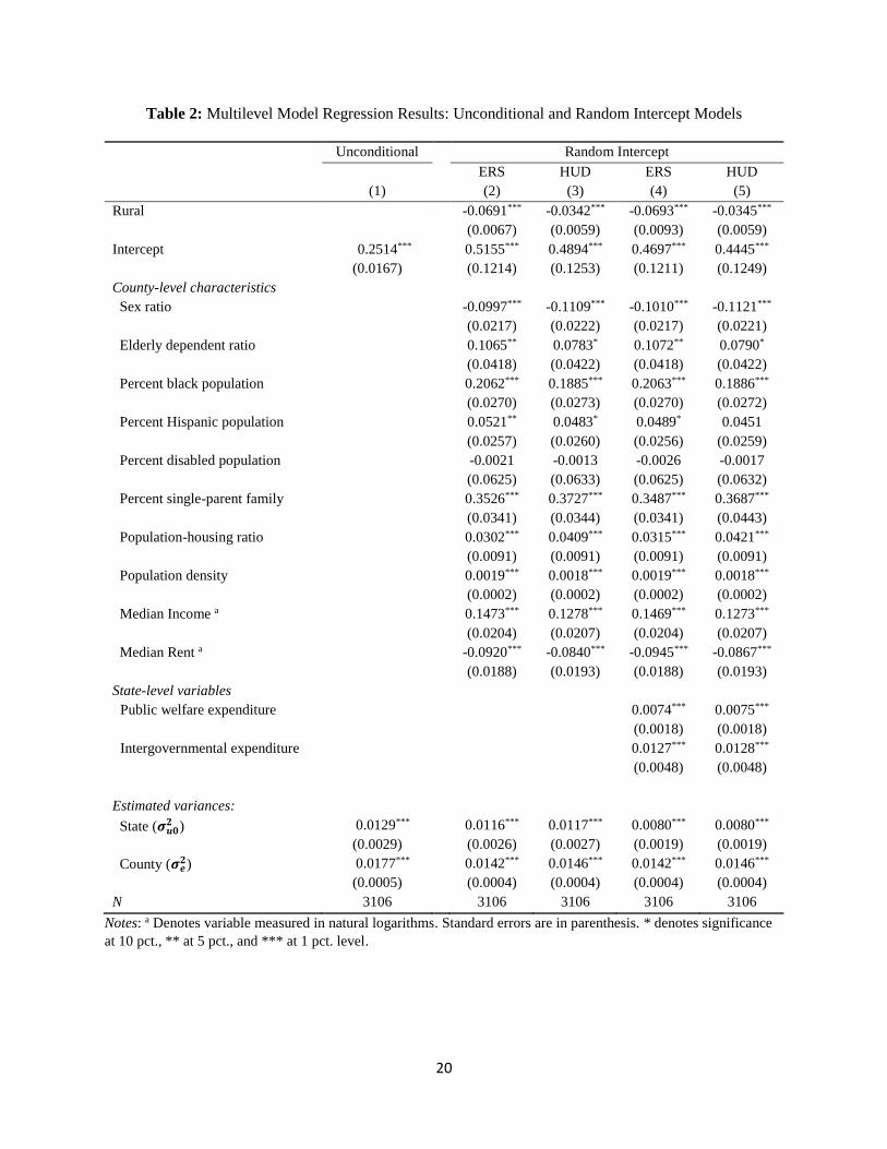
Results

Table 2 presents the results of three multilevel models of the geographical distribution of federally

funded rental subsidy programs. Column (1) presents results of the unconditional model that only

includes the intercept which varies across states. This preliminary information is useful in

providing Intraclass Correlation (ICC) coefficient estimated by the ratio of variance between states

(𝜎𝑢02 ) to the total variance (𝜎𝑢0

2 + 𝜎𝑒2). As can be seen in the column (1), the estimated variance, 𝜎𝑒

2,

12

is 0.0177 at county level, and at the level of states equals, 𝜎𝑢02 , 0.0129. The ICC is approximately

42.2 percent, and the remaining variation is at the county level (57.8 percent). The ICC shows that

a large amount of variance, attributed to the state-level, confirms that the two-level multilevel

models provide a better fit to the data.

Columns (2) and (3) report the results of the random intercept models with an inclusion of

the rural variable and the set of county-level control variables based on the two rural-urban

geographical classifications. With the exception of the percent disabled population variable, all

coefficients exhibit high levels of statistical significance. Specifically, using the ERS classification,

the negative coefficient of the rural variable indicates that rural residents in poverty are less likely

to receive federal rental subsidies by approximately 6.9 percentage points than those in urban areas;

and 3.4 percentage points lower with HUD’s rurality definition. Also, the results show that the

elderly-dependent ratio, proportion of minorities (black and Hispanic population), and single-

parent family are positively associated with the recipients-poor ratio. Additionally, population-

housing ratio, population density, and median income positively correlate, while sex ratio and

median rent negatively correlate with the recipients-poor ratio. Moreover, based on the estimates

of the random intercept model, we can predict the state-level random effects (unobserved

heterogeneity) to examine what extent the state influences the uneven administration of the current

federal rental subsidy programs. Since, in this model specification, we predict a random effect for

each state without state-level predictors, the interpretation of the results are straightforward.5

Based on the ERS definition, most states in the South region (i.e. Florida, Georgia, Mississippi,

and South Carolina) and some states in the West region (i.e. Arizona and Nevada) tend to have a

relatively lower-level of the recipients-poor ratio among 48 contiguous states; while some states

in the Northeast region (i.e. Connecticut, Massachusetts, New Hampshire, New Jersey, and Rhode

Island) and the Midwest region (South Dakota and Minnesota) are predicted to have a relatively

higher level of the recipients-poor ratio. 6

5 Because state random effect (𝑢0𝑗 ) measures a state-specific deviation from the state-mean outcome after

accounting for the effects of state-specific variables, the inclusion of additional state-level variables make the

interpretation difficult. 6 We observe very similar results of the predicted state effects (random intercepts) using the HUD’s rural

definition except slight changes in the magnitude of coefficients in South Dakota, Kansas, and Kentucky states.

13

In columns (4) and (5), we add state-level variables into the random intercept models. The

results show that state-level variables – the public welfare expenditure (per person in poverty) and

intergovernmental expenditure (adjusted by the number of counties within state) – are positively

associated with the recipients-poor ratio. Also, the inclusion of state-level variables explains about

an additional 31 percent of variance between states (𝜎𝑢02 ) relative to the estimated variances without

state-level variables reported in columns (2) and (3). However, these measures refer to variation

without random attributes existing across states. Estimating the random slope model can reveal a

state effect operating within the slopes as well. Specifically, we allow the rural variable to vary

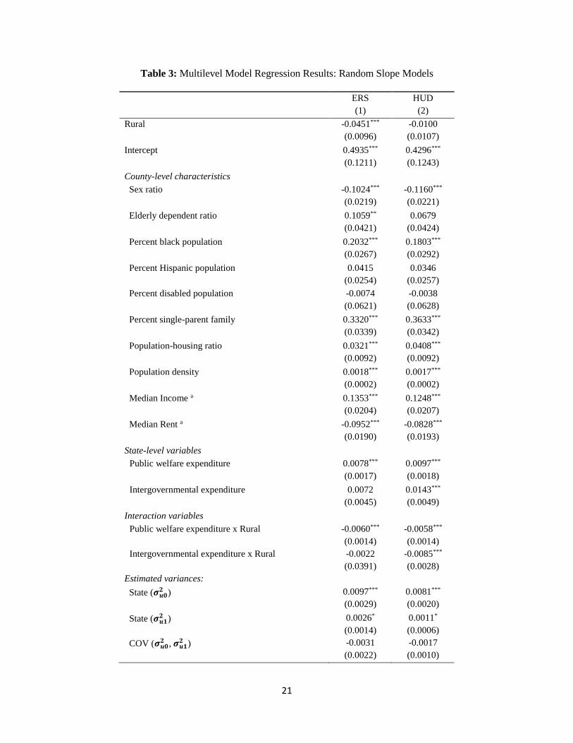
randomly across states in addition to state-level random intercepts (Table 3). Also, as we discussed

in Eq. (5), we add the interaction terms between rural variable (random slope variable) and state-

level variables into the regressions. In column (1), the results show that rural residents in poverty

are less likely to receive the rental subsidies by 4.5 percentage points after accounting for the

interaction terms (fixed effects) and random effects (random intercept and random slope), however,

using HUD’s rurality definition, the coefficient for rural variable still shows a negative sign but

most of the rural effects are absorbed into interaction terms (lose its statistical significance). Also,

we find that the multilevel random slope model reveals a statistical significance (at 10 percent

level of significance) of heterogeneous rural effects across states. Also, we find that both

interaction terms negatively correlate with the recipients-poor ratio, indicating that rural counties

tend to have a lower level of the recipients-poor ratio compared to the urban counties with the

same level of the state’s public welfare and intergovernmental expenditures. The rural context and

intergovernmental relationships explain these results.

If the state’s expenditures on public welfare programs and intergovernmental transfers to

local governments are concentrated in particular urban areas, the high level of such expenditures

(at the state level) does not necessarily alleviate poverty nor increase the number of rental subsidies

in rural areas. Indeed, in this case, rural poverty and inequality of the provision of federal rental

subsidies between rural and urban areas would become more severe. This story is plausible based

on findings in the previous literature. Undeniably, rural local governments may have insufficient

professionals, administrative capacity, and experience to obtain block grants and undertake

housing and community development initiatives (Reeder, 1996; Brown & Swanson, 2003). Also,

in economic return perspective, “federal funds are increasingly disbursed in the form of block

14

grants to the states, which can then decide whether they will invest in lagging rural communities

or in more economically vibrant communities that can serve as engines of economic growth”

(Brown & Swanson, 2003, p. 254). Under block grants, with less redistributing within a state, even

more rural local governments may fall behind.

Discussion

This paper uses multilevel modelling to analyze what extent of the rural-urban spatial

disproportionality exists in the current federal rental subsidy programs across all counties in the

48 continuous states. Our main findings suggest that rural residents in poverty are less likely to

receive the rental subsidies by approximately 3.4-7.1 percentage-points, based on different rural-

urban geographical classifications, than those in urban areas. Also, we understand the role of state

of particularly how states’ financial transfers, as well as state heterogeneity, are attributable to

uneven administration of the federal rental subsidy programs.

Our primary findings show a statistically significant program bias in the HUD public

housing subsidy programs against rural poor people. While 3.4 to 7.1 percentage points may not

appear to be a large effect size, the bias against rural poor people that we measure implies between

23,000 and 64,000 rural poor people do not receive services under the current program

implementation compared to a subsidized housing program implementation where rural people

were treated similarly to urban people. The within HUD housing program differential points to the

importance of the USDA housing and rental assistance programs, such as the Section 521 Rental

Assistance Program and the Section 515 financing program for developments that include low-

income households. Despite their importance as part of the rural housing safety net, these USDA

programs have experienced lower funding levels in recently, with reductions for the Section 521

Program in 2013 totaling 7.5% of the previous year’s funding level (Housing Assistance Council

[HAC], n.d.).

Because of the presence of USDA’s rural housing programs, our estimates represent an

upper bound on the size of the overall urban bias in public housing in the United States. That said,

significant variation in rural housing services exists at the state level, and public housing in general

15

faces a difficult financial future. All of these reasons point to the need for continued monitoring

and measurement of access to affordable housing in rural areas of the United States.

16

Reference

Albrecht, D. E. (1998). The industrial transformation of farm communities: Implications for

family structure and socioeconomic conditions. Rural Sociology, 63(1), 51-64.

Albrecht, D. E., & Albrecht, S. L. (2000). Poverty in nonmetropolitan America: Impacts of

industrial, employment, and family structure variables. Rural Sociology, 65(1), 87-103.

Brown, D. L., Swanson, L. E., & Barton, A. W. (2003). Challenges for rural America in the

twenty-first century. Rural Studies Series/Rural Sociological Society.

Conger, R. D., & Elder Jr, G. H. (1994). Families in Troubled Times: Adapting to Change in

Rural America. Social Institutions and Social Change. New York: Walter de Gruyter,

Inc.

Currie, J., & Yelowitz, A. (2000). Are public housing projects good for kids? Journal of Public

Economics, 75(1), 99-124.

DeNavas-Walt, C., & Proctor, B. D. (2015). Income and poverty in the United States: 2014.

United States Census Bureau. Retrieved from

http:// www.census.gov/content/dam/Census/library/publication/2015/demo/p60-252.pdf.

Devine, D. J., Gray, R. W., Rubin, L., & Taghavi, L. B. (2003). Housing choice voucher location

patterns: Implications for participant and neighborhood welfare. Washington, DC: U.S.

Department of Housing and Urban Development. Retrieved from

http://www.huduser.gov/publications/pdf/location_paper.pdf.

Duncan, C. M., & Coles, R. (2000). Worlds apart: Why poverty persists in rural America. Yale

University Press.

Falk, G. (2015). Low-Income Assistance Programs: Trends in Federal Spending. Congressional

Research Service (CRS), House Ways and Means Committee, United States Congress.

Retrieved from

http://www.greenbook.waysandmeans.house.gov/sites/greenbook.waysandmeans.houseg

ov/files/2012/documents/RL41823_gb.pdf.

Farrigan, T. (2015). Geography of Poverty. Economic Research Service (ERS), United States

Department of Agriculture (USDA). Retrieved from

http://www.ers.usda.gov/topics/rural-economy-population/rural-poverty-well-being.aspx.

Felix, A., & Henderson, J. (2010). Rural America’s Fiscal Challenge. Federal Reserve Bank of

Kansas City. Retrieved from http://kansascityfed.org/publicat/mse/MSE_0310.pdf.

Goering, J. M., Stebbins, H., & Siewert, M. (1995). Promoting housing choice in HUD's

rental assistance programs: Report to Congress. US Department of Housing and Urban

Development, Office of Policy Development and Research.

17

Goetz, E. G. (2003). Clearing the way: Deconcentrating the poor in urban America. The Urban

Institute.

Housing Assistance Council. (n.d.). USDA Rural Development Notifies Rural Rental Housing

Borrowers Regarding Section 521 Rental Assistance Shortfall. Retrieved from:

http://www.ruralhome.org/whats-new/mn-whats-new/45-announcements/726-usda-rural-

development-notifies-rural-rental-housing-borrowers-regarding-section-521-rental-

assistance-shortfall

Irwin, E. G., Isserman, A. M., Kilkenny, M., & Partridge, M. D. (2010). A century of research on

rural development and regional issues. American Journal of Agricultural Economics,

92(2), 522-553.

Jacob, B. A. (2004). Public Housing, Housing Vouchers, and Student Achievement: Evidence

from Public Housing Demolitions in Chicago. American Economic Review, 233-258.

Jacob, B. A., & Ludwig, J. (2012). The effects of housing assistance on labor supply: Evidence

from a voucher lottery. The American Economic Review, 272-304.

Jencks, C., & Mayer, S. E. (1990). The social consequences of growing up in a poor

neighborhood. Inner-city poverty in the United States, 111, 186.

Katz, L. F., Kling, J. R., & Liebman, J. B. (2001). Moving to Opportunity in Boston: Early

Results of a Randomized Mobility Experiment. Quarterly Journal of Economics, 607-

654.

Lens, M. C., Ellen, I. G., & O'Regan, K. (2011). Do vouchers help low-income households

live in safer neighborhoods? Evidence on the housing choice voucher program.

Cityscape, 135-159.

Massey, D. S., & Kanaiaupuni, S. M. (1993). Public housing and the concentration of poverty.

Social Science Quarterly, 74(1), 109-122.

National Rural Housing Coalition (NRHC). (2014). Rural America’s Rental Housing Crisis.

Washington, DC.

Newman, S. J., & Schnare, A. B. (1997). … And a suitable living environment: The failure

of housing programs to deliver on neighborhood quality. Housing Policy Debate, 8(4),

703-741.

Newman, S. J. (2005). Low-end rental housing: The forgotten story in Baltimore's housing

boom.

Urban Institute. Retrieved from

http://www.urban.org/research/publication/low-end-rental-housing

18

Pendall, R. (2000). Why voucher and certificate users live in distressed neighborhoods.

Housing Policy Debate, 11(4), 881-910.

Reeder, R. J. (1996). How Would Rural Areas Fare Under Block Grants? (No. 33609). United

States Department of Agriculture, Economic Research Service.

Rice, D., & Obama’s, W. P. (2009). What to look for in HUD’s 2010 budget for low-income

housing. Center on Budget and Policy Priorities, 5.

Ricketts, T. C. (1999). Rural health in the United States. New York: Oxford University Press.

Schwartz, A. F. (2014). Housing policy in the United States. New York: Routledge.

Tickamyer, A. R., & Duncan, C. M. (1990). Poverty and opportunity structure in rural America.

Annual Review of Sociology, 67-86.

Turner, M. A. (1998). Moving out of poverty: Expanding mobility and choice through

tenant‐based housing assistance. Housing Policy Debate, 9(2), 373-394.

Von Hoffman, A. (1996). High ambitions: The past and future of American low‐income housing

policy. Housing Policy Debate, 7(3), 423-446.

____________. (2012). History lessons for today's housing policy: the politics of low-income

housing. Housing Policy Debate, 22(3), 321-376.

Wilson, W. J. (1987). The Truly Disadvantaged: The Inner City, the Underclass, and Public

Policy. Chicago: Univ. Press, Chicago.

U.S. Bureau of Census. (n.d.). State Government Finances. Available at:

https://www.census.gov/govs/state/. Accessed December 15, 2015.

U.S. Bureau of Census. (2008). A compass for understanding and using American Community

Survey data: What general data users need to know. Census Bureau. Retrieved from

http//www.census.gov/content/dam/Census/library/publications/2008/acs/ACSGernealHa

ndbook.pdf.

19

Tables

Table 1: Descriptive Statistics of Selected Rural and Urban Characteristics

All Counties

ERS HUD

Rural Urban Rural Urban

Poverty Rates 0.159

(0.060)

0.165

(0.067)

0.157

(0.058)

0.171

(0.063)

0.146

(0.054)

Recipients-Poor Ratio 0.222

(0.150)

0.155

(0.138)

0.239

(0.148)

0.193

(0.138)

0.255

(0.157)

County-level variables

Sex ratio 1.004

(0.109)

1.034

(0.143)

0.997

(0.097)

1.024

(0.129)

0.982

(0.074)

Elderly dependent ratio 0.275

(0.086)

0.348

(0.094)

0.256

(0.072)

0.310

(0.083)

0.236

(0.069)

Percent black population 0.091

(0.146)

0.061

(0.145)

0.098

(0.145)

0.078

(0.153)

0.104

(0.136)

Percent Hispanic population 0.085

(0.134)

0.059

(0.111)

0.092

(0.139)

0.078

(0.138)

0.093

(0.129)

Percent disabled population 0.140

(0.052)

0.154

(0.063)

0.136

(0.049)

0.154

(0.056)

0.125

(0.042)

Percent single-parent family 0.300

(0.102)

0.272

(0.125)

0.307

(0.094)

0.300

(0.111)

0.303

(0.090)

Population-housing ratio 2.165

(0.371)

1.864

(0.395)

2.240

(0.323)

2.025

(0.382)

2.321

(0.287)

Population density 219.012

(1245.18)

14.305

(15.491)

270.684

(1388.768)

32.404

(92.871)

428.850

(1789.466)

Median Income (/104) 4.575

(1.180)

4.135

(0.872)

4.687

(1.221)

4.135

(0.850)

5.071

(1.296)

Median Rent (/102) 6.786

(1.847)

5.563

(1.135)

7.094

(1.865)

5.883

(1.118)

7.800

(1.975)

State-level variables

Public welfare expenditure

(/ persons in poverty)

10.393

(3.613)

9.951

(2.611)

10.505

(3.817)

10.112

(2.962)

10.709

(4.206)

Intergovernmental expenditure

(/ number of counties in state; /106)

1.565

(2.512)

0.845

(1.404)

1.747

(2.692)

1.113

(1.771)

2.074

(3.066)

N 3106 626 2480 1644 1462

Note: Standard deviations are in parenthesis.

20

Table 2: Multilevel Model Regression Results: Unconditional and Random Intercept Models

Unconditional Random Intercept

(1)

ERS

(2)

HUD

(3)

ERS

(4)

HUD

(5)

Rural -0.0691***

(0.0067)

-0.0342***

(0.0059)

-0.0693***

(0.0093)

-0.0345***

(0.0059)

Intercept 0.2514***

(0.0167)

0.5155***

(0.1214)

0.4894***

(0.1253)

0.4697***

(0.1211)

0.4445***

(0.1249)

County-level characteristics

Sex ratio -0.0997***

(0.0217)

-0.1109***

(0.0222)

-0.1010***

(0.0217)

-0.1121***

(0.0221)

Elderly dependent ratio 0.1065**

(0.0418)

0.0783*

(0.0422)

0.1072**

(0.0418)

0.0790*

(0.0422)

Percent black population 0.2062***

(0.0270)

0.1885***

(0.0273)

0.2063***

(0.0270)

0.1886***

(0.0272)

Percent Hispanic population 0.0521**

(0.0257)

0.0483*

(0.0260)

0.0489*

(0.0256)

0.0451

(0.0259)

Percent disabled population -0.0021

(0.0625)

-0.0013

(0.0633)

-0.0026

(0.0625)

-0.0017

(0.0632)

Percent single-parent family 0.3526***

(0.0341)

0.3727***

(0.0344)

0.3487***

(0.0341)

0.3687***

(0.0443)

Population-housing ratio 0.0302***

(0.0091)

0.0409***

(0.0091)

0.0315***

(0.0091)

0.0421***

(0.0091)

Population density 0.0019***

(0.0002)

0.0018***

(0.0002)

0.0019***

(0.0002)

0.0018***

(0.0002)

Median Income a 0.1473***

(0.0204)

0.1278***

(0.0207)

0.1469***

(0.0204)

0.1273***

(0.0207)

Median Rent a -0.0920***

(0.0188)

-0.0840***

(0.0193)

-0.0945***

(0.0188)

-0.0867***

(0.0193)

State-level variables

Public welfare expenditure

0.0074***

(0.0018)

0.0075***

(0.0018)

Intergovernmental expenditure

0.0127***

(0.0048)

0.0128***

(0.0048)

Estimated variances:

State (𝝈𝒖𝟎𝟐 ) 0.0129***

(0.0029)

0.0116***

(0.0026)

0.0117***

(0.0027)

0.0080***

(0.0019)

0.0080***

(0.0019)

County (𝝈𝒆𝟐) 0.0177***

(0.0005)

0.0142***

(0.0004)

0.0146***

(0.0004)

0.0142***

(0.0004)

0.0146***

(0.0004)

N 3106 3106 3106 3106 3106

Notes: a Denotes variable measured in natural logarithms. Standard errors are in parenthesis. * denotes significance

at 10 pct., ** at 5 pct., and *** at 1 pct. level.

21

Table 3: Multilevel Model Regression Results: Random Slope Models

ERS

(1)

HUD

(2)

Rural -0.0451***

(0.0096)

-0.0100

(0.0107)

Intercept 0.4935***

(0.1211)

0.4296***

(0.1243)

County-level characteristics

Sex ratio -0.1024***

(0.0219)

-0.1160***

(0.0221)

Elderly dependent ratio 0.1059**

(0.0421)

0.0679

(0.0424)

Percent black population 0.2032***

(0.0267)

0.1803***

(0.0292)

Percent Hispanic population 0.0415

(0.0254)

0.0346

(0.0257)

Percent disabled population -0.0074

(0.0621)

-0.0038

(0.0628)

Percent single-parent family 0.3320***

(0.0339)

0.3633***

(0.0342)

Population-housing ratio 0.0321***

(0.0092)

0.0408***

(0.0092)

Population density 0.0018***

(0.0002)

0.0017***

(0.0002)

Median Income a 0.1353***

(0.0204)

0.1248***

(0.0207)

Median Rent a -0.0952***

(0.0190)

-0.0828***

(0.0193)

State-level variables

Public welfare expenditure

0.0078***

(0.0017)

0.0097***

(0.0018)

Intergovernmental expenditure

0.0072

(0.0045)

0.0143***

(0.0049)

Interaction variables

Public welfare expenditure x Rural

-0.0060***

(0.0014)

-0.0058***

(0.0014)

Intergovernmental expenditure x Rural

-0.0022

(0.0391)

-0.0085***

(0.0028)

Estimated variances:

State (𝝈𝒖𝟎𝟐 ) 0.0097***

(0.0029)

0.0081***

(0.0020)

State (𝝈𝒖𝟏𝟐 ) 0.0026*

(0.0014)

0.0011*

(0.0006)

COV (𝝈𝒖𝟎𝟐 , 𝝈𝒖𝟏

𝟐 ) -0.0031

(0.0022)

-0.0017

(0.0010)

22

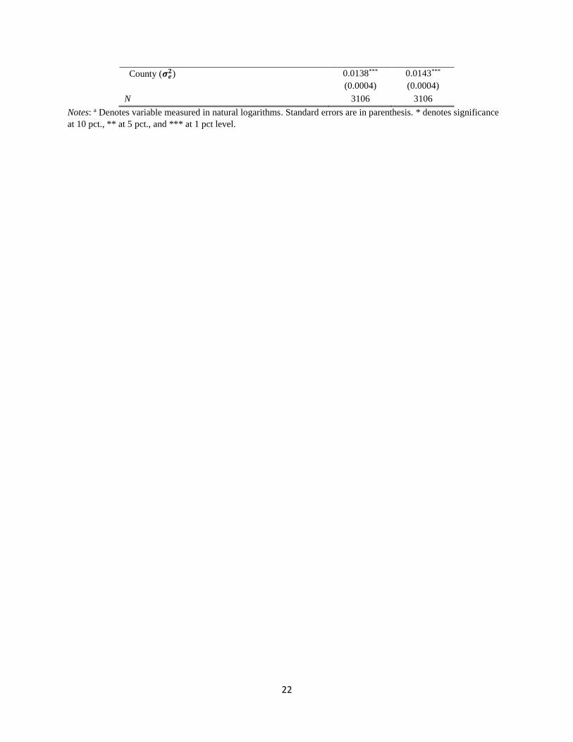
County (𝝈𝒆𝟐) 0.0138***

(0.0004)

0.0143***

(0.0004)

N 3106 3106

Notes: a Denotes variable measured in natural logarithms. Standard errors are in parenthesis. * denotes significance

at 10 pct., ** at 5 pct., and *** at 1 pct level.