are rich and poor equally represented by lawmakers...

How Poorly are the Poor Represented in the US Senate?

Robert S. Erikson

Professor of Political Science Columbia University

726 IAB, 420 W. 118th St. New York, NY 10027

Yosef Bhatti Department of Political Science

Øster Farimagsgade 5, 1353 København K University of Copenhagen

Chapter prepared for Enns, Peter and Christopher Wlezien (eds.): “Who Gets Represented”, New York: Russell Sage Foundation

Abstract

In his new book Unequal Democracy, Larry Bartels finds that rich constituents are substantially better represented by the legislators in the US Senate than their poorer counterparts. In fact, the poorest third of the population is not represented at all. While we do not find evidence directly contradictory this result, we add some complications. First, we solve a methodological problem caused by the fact that the weights used in the existing literature render the results scale variant. Second, we replicate Bartels’ findings in two recent datasets with larger sample sizes and hence less measurement error. We cannot find statistical evidence of differential representation. A contributing reason is that ideological preferences among different income strata of state electorates are almost impossible to separate statistically.

Introduction

In his widely (and justly) acclaimed new book, Unequal Democracy, Larry

Bartels (2008) presents the case that the rich get more representation than the poor.

Among other findings, we learn that Republican administrations serve to advance income

inequality rather than retard it. And we learn that Republicans are capable of fooling

voters, although not for the reasons that Thomas Frank (2004) offers in What’s the Matter

with Kansas? Among the most provocative findings is that when it comes to

representation in the US Senate (as measured by roll call voting), the poor—unlike the

well-to-do—get virtually no representation at all. That is, when Senators take into

account (or respond in some indirect fashion) to public opinion, only the views of the

relatively rich and—to a lesser extent middle-income voters—matter. Based on Bartels’

statistical analysis, the views of the relatively poor are not visibly represented at all.

In terms of senatorial representation, is political inequality as severe as Bartels

makes out? While one would certainly expect that affluence would have something to do

with influence over Congress, the degree of inequality reported by Bartels is stronger

than one might expect to be the case. In this paper we investigate further. We replicate

and extend Bartels’ analysis, while presenting certain methodological hurdles that hinder

a decisive verdict. In the end, this paper does not challenge Bartels’s finding of unequal

representation as necessarily incorrect. However we do offer what we believe to be

compelling reasons to interpret the evidence with considerable caution.

Some Theory

Before turning to the statistical evidence, it is helpful to review the reasons why

senatorial representation would be expected to be unequal. That is, why would Senators

1

be more responsive to the opinions of the rich than the poor? Bartels mentions several

reasons. The rich are more attentive and more likely to vote. Second, the rich are more

likely to contribute to campaigns. For these reasons, reelection-seeking Senators have

reason to pay more attention to rich opinion than to poor opinion. Moreover, Senators are

themselves from the social strata of the relatively rich. To some extent, they would share

the views of the relatively rich and interact with constituents who themselves are

relatively rich. To the extent that the poor are invisible to Senate members, it is unlikely

that Senators consider the views of the poor.

At the same time, as Bartels acknowledges, these are only relative differences.

The statistical analysis suggests that the top third in income gets most of the

representation while the bottom third gets none. Many citizens in the bottom third vote

and many in the top third do not. While the relatively affluent give more to campaigns, it

is an elite strata of the top third in income—who give the most. These considerations

make it puzzling that the gap in representation between the moderately rich and

moderately poor is as great as Bartels’ statistical analysis would suggest.

There is also another consideration. Following the lead of Miller and Stokes’

(1963) classic study of congressional representation, political scientists are prone to

discuss representation as a phenomenon that is solely due to the actions of the

representatives. When scholars theorize about why legislators represent (or not represent)

constituency opinion, the focus usually is on the supply side—why, deliberately or

incidentally, legislators end up following constituency wishes. The demand side should

not be ignored. Voters also play a role. At least potentially, they sort candidates into

winners and losers in part based on their ideological proximity to the candidates. At a

2

minimum, members of Congress—including Senators—behave as if they believe this to

be true. Otherwise they would be indifferent to constituency representation. Political

scientists—going back to Miller and Stokes’ classic works—sometimes write as if

legislators overestimate constituency attention to their behavior. While this is possible,

one could also bring forward a “rational expectations” argument that legislators do not

make systematic mistakes. That is, given their relative utilities for voting correctly in

terms of their personal ideological values and voting to stay elected, representatives

weigh the goals correctly in terms of maximizing their long-term welfare.

The implication of this line of theorizing is that legislators know what they are

doing. If they respond to public opinion generally (as they seem to do), they respond with

good reason rather than with unjustified inflation of their visibility to constituents. But if

we take Bartels’ finding of differential representation seriously, then legislators rationally

ignore the poor. For such behavior to be rational, Senators are indeed invisible to the poor

while sufficiently visible to the well-to-do for Senators to give the rich their attention. To

come full circle, for Senators to ignore the poor is rational only if the poor ignore their

Senators.

Based on Bartels’ analysis it is unlikely that Senators overestimate the attention

they receive from their poorer constituents. But consider the opposite—a world where

Senators mistakenly ignore the poor while the poor do pay attention and—just like their

affluent counterparts—vote their legislators in or out based on the proximity of candidate

positions to their own. The outcome is the positive representation of poor constituents, as

the poor have some ability to elect and keep Senators who share their views and reject

those who do not.

3

The net result of this theorizing is that for it to make sense for the poor to get no

representation of their views in the Senate, the poor must indeed be inattentive to their

Senators. If Bartels’ research is correct, the implication is not only that Senators freely

ignore the views of the poor. The poor must ignore the fact that they are not represented.

Bartels’ Analysis and Replication

Bartels’s analyses the relationship between state opinion and senatorial liberalism

for three Congresses following the elections of 1988, 1990, and 1992. These Congresses

were chose because the 1988, 1990 and 1992 elections were the venue for the American

National Election Study’s “Senate” study in which the respondents in larger than usual

state samples were interviewed for the purpose of analyzing senatorial representation.

The Senate study was designed to provide equal sample sizes in each state, resulting in an

average of 185 respondents per state ranging between 151 and 223.1

To estimate the degree of Senate representation in general, Bartels modeled

Senator conservatism (the first dimension of Poole and Rosenthal’s W-nominate scores)

on party affiliation and the state mean self-identification on a rescaled version of the NES

7-point ideology question.

As Bartels’ analysis makes clear (see Figure 9.1 on page 256), state public

opinion is a strong predictor of senatorial roll call ideology, even with the Senator’s party

affiliation controlled. We show this strong relationship in Table 1, where both

partisanship and state ideology (measured as Bartels does from the NES Senate study) are

strong predictors of W-nominate first dimension scores over the three Congresses

following the 1988, 1990, and 1992 election.

1 The numbers drops slightly when we take into account non-respondents to the ideology question and its follow up. Thus, an average of 171 valid respondents could be used in the analysis, ranging from 138 to 209.

4

[Table 1 about here]

The general fact that state opinion influences roll call behavior is not in question.

At issue is the equality of the representation process. Do some opinions matter more than

others? Specifically, is it mainly the opinions of the affluent that count?

After first demonstrating that state opinion matters for Senate roll call voting,

even with Senator party controlled, Bartels turns to the test that is crucial for this

discussion. Bartels separates opinion by the lowest third, the middle third, and the highest

third on family income where the thirds are defined by the national division. That is,

separate mean ideologies are calculated for each of three income groups in each state.

The lowest group is composed of individuals with a family income below $20,000, in the

middle-income group the income ranges from $20,000 to $40,000, while respondents

with family income above $40,000 are assigned to the high-income group. Using a

methodological principle that has been employed elsewhere (e.g., Erikson et al. 1993;

Clinton 2006), Bartels decomposes state opinion into three separate variables: The

notation is ours.

Low-income ideology times proportion in the low-income category:

LL PX_

Middle-income ideology times the proportion in the middle-income category

MM PX_

High-income ideology times proportion in the high-income category

HH PX_

5

Where = mean ideology among the income group G within the state sample and =

the proportion within the sample in income group G. Had Bartels only measured Senator

ideology as a function of the raw mean group ideologies ( ), he would had captured

the Senators’ responsiveness to the actual groups in the population which varies across

states. Hence, the purpose multiplying the proportions ( ) with the raw mean group

ideologies ( ) is to take into account the different sizes of the groups in the electorate

and thereby to create a common baseline for comparison. Bartels measures ideology by

recoding scores on the original NES seven point 1-7 scale into a scale from -1 to +1. The

original “1” becomes -1; the original “7” becomes +1, etc. The midpoint shifts from 4 to

zero, a seemingly innocuous shift that becomes salient in the discussion below.

GX_

GP

GX_

GP

GX_

To sum up, with individual Senators as the unit of analysis, Bartels match the first

dimension of the W-nominates (dependent variable) with subgroup constituency

ideologies weighted by the proportion of the groups in each state. A Republican Senator

dummy is added to allow for party-specific behavior independent of constituency

influence.


We show Bartels’ original finding for the pooled 101-103 Congresses in Table 2,

column 1. Senate W-nominate scores are highly responsive to party plus high-income

opinion and (to a lesser extent) middle-income opinion. But for the low-income third, the

coefficient is non-significant and actually negative in sign. This is the crucial finding that

suggests that for poor folks, there is no representation in the upper chamber of Congress.

6

When we try to replicate Bartels’ equation, we come passably close, as shown in

column 2 of Table 2. So this is the starting point of our investigation. Would further

analysis lead to the discovery of anything different? The first step of our investigation

was a seemingly innocuous variation. We repeated the model with the only change being

a rescaling of the key independent variables on the original scale of 1 to 7 rather than -1

to +1. The results are in column 3 of Table 2.

One’s first thought is that the equations of column two and three should be

identical except for the matter of scale since scores on the -1 to +1 scale correlate

perfectly with the scores on the 1 to 7 scale. One can refer back to Table 1 to see that this

is true about total opinion. When the scale range is stretched by a factor of three from 2

points (-1 to +1) to 6 points (1-7 rather than 2 points (-1 to +1)), the coefficients are

identical except for the proportional shrinkage of the opinion coefficient by one third.

But when opinion is measured separately by income group, as in Table 2, scale

matters. Observe first that by replacing the -1 to +1 scale with the 1 to 7 scale, the

explained variance (adjusted R squared) actually declines slightly from .85 to .83.

Crucially, the relative sizes and significance levels of the three components of state

opinion also changed. Taking the equation in column 3 at face value, opinion is about

equally influential among low-income, middle-income, and high-income families.

Moreover, the coefficients are “statistically significant” at the .001 level for all three

income groups. Thus by measuring ideology on a 7 point scale instead of a 2 point scale,

we have transformed our result into one approaching a utopia of equal and strong

ideological representation.

7

Clearly something is amiss. The problem lies in the algebra with which the

independent variables in Table 1 are constructed. Recall that our three opinion variables

are each a multiplicative term, with the within-group state mean multiplied by the

proportion of the state sample within the group category. When we modify the original

measures of state’s income-category mean opinion by adding or subtracting a constant for

all values, we transform so that the initial coefficients for ideology effects (depicted

below as betas) change to represent the composite weighted contribution of group

ideology plus the proportion in the group (depicted below as gammas).

Let us examine algebraically what happens when we add an arbitrary constant (k)

to the state mean and thus replace the original set of estimates of relative state opinion

effects (the βs) with the new ones (the γs).

For low-income ideology,

is replaced by LLL PX_

β )()(__

LLLLLLL kPPXPkX +=+ γγ

For middle-income ideology,

MMM PX_

β is replaced by )()(__

MMMMMMM kPPXPkX +=+ γγ

And similarly, for high-income ideology,

HHH PX_

β is replaced by )()(__

HHHHHHH kPPXPkX +=+ γγ

As long as the and ”effects” are zero, adding the constant makes no

difference. But they will not be zero, because these “effects” are the accounting

mechanisms that anchor the equation when the state mean and proportion within the

income category are “zero.” By arbitrarily adding or subtracting a constant k, one can

,, ML PP HP

8

change the order and the signs of the relative effects ideology within the three income

categories. We have already seen this when we shift from a -1 to +1 range for ideology to

a 1 to 7 range. The culprit is not the expansion of the range from 2 to 6 points, but rather

the shift of the “midpoint” from zero to four.

The problem is readily solved, however, by simply incorporating the proportions

in the categories as additional variables. With three categories, adding the proportion

low-income and the proportion high-income are sufficient as they perfectly define the

proportion in the middle as the portion left over from one hundred percent. With this step,

adding an arbitrary constant will not affect the estimate of the relative contributions of

income categories. The relative effects of ’s become scale invariant. The relative

effects of the ’s however will indeed vary, as they remain conditional on the

(arbitrary) choice of zero point. Thus any substantive interpretation of the relative

coefficients must be conditional on the location of the zero points on the scales.

GG PX_

GP

GP

GG PX_

We see the result of adding coefficients for the ’s in Table 3. The new table

appears to validate Bartels’ original finding: With proportions in the low-income and

high-income category controlled, the relative impact of ideology within the state appears

to be highest for high-income voters, next highest for middle-income voters, and

nonexistent (actually negative) for low-income voters. The two sets of estimates are now

equivalent with the 1-7 estimates being exactly three times those with the -1 to +1 scale.

GP


We have also replicated Bartels’ separate analyses of Democrats and of

Republicans while adding as independent variables the proportion high-income and the

9

proportion low-income. As before, the estimated impact of high-income opinion is

positive and significant; the estimated impact of middle-income opinion is also but less

so; and the estimated impact of low-income opinion is trivial and actually negative. So

like Bartels, our replication finds that even Democratic Senators appear unresponsive to

low-income opinion. We also performed separate analyses excluding the South, and

excluding the south separately by party of the Senator. In each case the essential findings

are unmoved.

So far, our analysis supports Bartels. Analyzing the same NES Senate data as he

did, we find considerable evidence for public opinion influencing roll call behavior, but

only for citizens of sufficiently high-income. We should not lose sight of the fact that

opinion generally seems influential (Table 1); it is just that some opinions count more

than others.

For further understanding, we replicated a step that Bartels reports in a footnote.

Instead of dividing state samples into three groups based on the national income division,

we divided each states into thirds based on income within the state, allotting each group

(low-income, middle-income, and large income) as close to one third of the sample of

opinion-holders as possible. Then we ran a simple regression predicting roll call W-

nominate scores from Senator party affiliation plus mean scores in each state’s lowest

third, middle third, and highest third in terms of family income. The advantage is that

these results require no correction by proportion since each state’s sub-samples are

designed to be roughly equal in size.


10

Table 4 shows the results. The first and second column shows an equation

predicting W-nominate scores from the Senator’s party plus the mean ideology of each of

the three income groups in the NES sample. We see once again that high-income

respondents appear to matter but not low-income respondents. The difference is that this

time respondents’ placement in their income category is based on their income relative to

income of other families in their home state rather than their classification in the national

income breakdown.

An important issue when using survey generated means to predict legislative

behavior is the measurement error in the ideology variables. Large as the samples are for

the NES Senate study, their use produces wobbly estimates when the data is sliced by

income groups. The mean N’s for the low-income, medium income, and high-income

samples are, respectively, only 48, 68, and 54 cases per state. We draw on sampling

theory to estimate the measurement error and reliability of the three sets of ideology

scores based on states’ N’s and within-state variances and the observed between-state

variances. Reliability estimates for these data suggest that less than more than half the

variance of the three income group means is actually sampling error rather than variance

in true state means - more specifically, the reliabilities are .41, .48 and .50 for the low-

income, middle-income and high-income groups respectively.2

This assessment represents both bad news and good news. The bad news is that

estimates of the effects should be taken as more uncertain than the coefficients in Tables 2 We calculated the reliability for the three groups using the following formula based on sampling theory: Reliability= (total variance-error variance)/total variance. The total variance is simply the observed between-state variance, i.e. the variance of state ideology means of the group in question across states. The error variance is the within-state variance. It is obtained by first taking the variance for the group in question in each state and divide with the number of valid observations for that group in the states. Then the mean is taken of these state-specific within variances. The intuition is the greater variance between states compared to the (within-state) error variance, the higher reliability.

11

1-4 would suggest. The good news is that in general, the measurement error attenuates

the relationships so that the error must tilt in the direction of underestimation of the

magnitudes of state opinion effects. In short, we should expect even more representation

generally than reported so far in these pages.

The reliabilities are in this case unfortunately too small to run errors-in-variables

regression. This calls for further examination, using dataset with higher sample sizes with

the purpose of obtaining higher reliabilities. Thus, below we examine Bartels’ findings

using two large recent datasets, namely the Annenberg surveys 2000-2004 and exit poll

data from the 2004 election.

New Data I: Annenberg 2000-2004

We replicated the findings from the Senate study by pooling the Annenberg

surveys from 2000 and 2004. The advantage of the Annenberg surveys compared to the

Senate study is that they provide us with extremely high sample sizes and hence less

measurement error in the main independent variables. When the 2000 and 2004 surveys

are pooled, a total of 155,000 respondents are available. This is a substantial

improvement compared to the 9,253 respondents available to Bartels. Thus, we can

expect the income-specific mean ideology scores to be estimated with a much higher

reliability with this new dataset. Furthermore, using the Annenberg surveys allows us to

test Bartels’ findings across time (1999-2005 compared to 1989-1995). The downside of

this new dataset is that it was sampled nationally and not state-wise as the NES Senate

study, resulting in very unequal sample sizes across states.3

3 The state-level sample sizes varied between 344 (Wyoming) and 15,419 (California) in the Annenberg pooled file, while ranging between 151 (New York) and 223 (Idaho) in the Senate study.

12

As in the previous analysis, we recode the original 5-point measure to range

between -1 and 1. In the interest of space, only the recoded measure will be presented

below. For comparison with Bartels, the dependent variable is still the 1st dimension of

W-nominates. As with NES Senate data, using the Annenberg data results in a strong

effect of state opinion on roll calls (Table 5).4 It is the equality of opinion that is at issue.

[Tables 5, 6 about here]

In Table 6 we have applied the methodology from Bartels (2008) to the

Annenberg surveys. At first sight, the results seem to verify the findings from Table 3.

There is statistical evidence that Senators are representative of high-income ideology,

while the coefficient for the poorest third is insignificant. However, a Wald test for the

difference between low-income representation and high-income representation fails the

.05 threshold. That is, we cannot find statistical evidence for a difference between the

low-income and high-income group.

Now why is that? If we compare the Annenberg results with the Senate study, two

main differences emerge. First, though still insignificant, the low-income ideology now

has a positive coefficient. Second, and most important, the standard errors of the

coefficients are more than twice in magnitude compared to the 1989-1995 results. This

can be ascribed to the fact that the income categories are much more internally correlated

in the Annenberg data (low-middle 64, low-high .67 and middle-high .86) than in the

Senate study (low-middle .31, low-high .31 and middle-high .33).5 This results in higher

multicollinearity and thus higher standard errors.

4 We examine the 106th to 108th Congresses instead of 107th-109th since W-nominate scores are not at the time of writing available for the 109th Congress. This should be inconsequential for the results. 5 When corrected for reliability, the correlations among the ideology scores for the income groups in the Senate study are approximately twice as high as observed.

13

The results are substantively equivalent when we base the income groups upon

state-specific definitions (Table 7, column 1). High-income ideology is the only

significant ideology variable but is not significant differently from low-income ideology.

As in table 4 we exclude the proportions, since each group approximately contains one-

third of the respondents in each state.


An advantage of the Annenberg data compared to the NES Senate study is the

higher reliabilities which allows us to run errors-in-variables regression (Table 7, column

2). Using sampling theory, reliabilities of .70 (low-income), .88 (middle-income) and .95

(high-income) are obtained. The differences in the reliabilities are mainly due to lower

true variance in the low-income group than in the two other groups. The lower reliability

for low-income could mean that it is differentially attenuated, i.e. that part of tendency

towards larger high-income coefficient is a statistical artefact.

When errors-in-variables regression is applied (Table 7, column 2), the

coefficients increase somewhat in magnitude, and the relative difference between low-

income and high-income decrease further. Additionally, multicollinearity becomes even

more severe as the error-corrected correlations between the income groups are as high as

.82 (low-middle), .82 (low-high) and .94 (middle-high). This adds to the impression that

the income groups are too closely related to statistically separate their individual impact

and that robust statistical evidence for uneven representation therefore cannot be found in

the Annenberg data.

New Data II: The 2004 Exit Polls

14

As a further data set, we replicate the Senate study findings using the 2004 state

exit polls. For this part of the analysis, we also experiment with different dependent

variables to check the robustness of the results across policy dimensions. More

specifically, we use three measures of Senator ideology in the 109th Congress: Pool and

Rosenthal’s DW-nominate scores on dimension 1, DW-nominate scores on dimension 2,

and a composite, weighing the second dimension .0.35 the amount of the first (.74 times

dimension 1 and .26 times dimension 2).

The advantage of the exit poll dataset is that the large state samples allow an

expansion of the state N’s to an average of 1350 (summed across income categories) and

a minimum of 584. Thus most Ns per income category are in the multiple hundreds, an

advantage over the Annenberg study with its more uneven set of N’s per state. One

obvious difference from the NES Senate data and the Annenberg data is that exit polls are

limited to voters only. Also, the exit poll mean ideology scores are based on a 3 point

scale, where respondents are only allowed to declare themselves as liberals, moderates, or

conservatives, with no categories in-between. As in the previous part, we calibrate this

ideology scale to range from -1 to 1.


Table 8 displays the estimated effects for dependent variables, using the national

income categories6 and weighting within-category means by their proportions. Relating

Senate ideology to opinion within income groups in the 2004 exit polls, we find some

pattern of senatorial responsiveness to opinion. However, while the coefficients for all

6 Low-income voters are defined as under $30,000 in family income (22 percent). High-income voters are defined as those with $75,000 or over in family income (33%). The remainder who revealed their income were coded as middle-income voters. We used the $30,000 threshold to distinguish low-income voters from middle-income voters even though it reduces the low-income percent to barely over one fifth because the next highest income category in the questionnaire ($30-$50 K) contains 22 percent of all voters.

15

three groups for all three versions of the dependent variable are positive, they are most

positive for low-income opinion. This is an outcome that does not seem right, and will be

challenged below. One possibility is that breaking down exit poll opinion by income

group adds virtually nothing to the prediction of Senator behavior.


Consider that if we substitute ideological means for the entire state sample (Table

9) we obtain not only highly significant coefficients but also virtually the same explained

variance as when parsing by income. When each of the three dependent variables of

Table 8 is predicted from party and net state ideology alone, the adjusted R squared is

within a point or two of those shown with the more elaborate model.

As for Annenberg, the main problem with the Senate exit poll data is that mean

ideology scores for the three income categories were highly correlated (.85 low-

middle,75 low-high and .90 middle-high). That is, the three income groups move

together. If a state is liberal, all three groups are relatively liberal; if it is conservative, all

three groups are relatively conservative. This extreme multicollinearity rendered

problematical any attempt to separate the effects of opinion across income groups. The

problem is even slightly worse when measurement error is taking into account.7

A different but also odd verdict arises when exit poll respondents are classified by

thirds of income within their state. For this exercise we divide the state exit poll

electorate into precise thirds for the division into low, medium, and high-income

respondents. We do it in a slightly refined way compared to in the previous sections.

When voters in an income category span the percentile threshold between the first and

7 The error-corrected pair-wise correlations are .95 (high-middle), 92 (middle-low) and .80 (high-low). In the interest of space, we do not present eivreg results which only amplify our conclusions.

16

second or the second and final third of the income categories, their group identity is

assigned proportionally. For instance when voters in an income category are between the

27.3 and 35.3 percentile, they are assigned .75 to the low-income group and .25 to the

middle-income group. The advantage of doing it this way is that the proportions within

each group by construction become exactly .333. The correlations of state ideology

across these three groups remain high—between .83 and .91.

[Table 10 about here] Table 10 shows the results. If one differentiates one group that is least influential

from Table 10 it is low-income voters. On the presumably most salient first dimension,

middle-income ideology appears as most influential, but the positive coefficient is not

statistically significant. High-income voters have a particularly positive (and significant)

coefficient on the second dimension, as if this dimension - dealing with issues such as

civil rights and civil liberties - has special significance to high-income voters.

We should not, however, put much weight on the results of either Table 8 or

Table 10. In only one of the six equations, are the three ideology variables significantly

different from each other. Oddly, that is for the composite measure of roll call ideology in

Table 8. In general, the coefficients vary widely but with large standard errors that

dampen confidence in the estimates. The collinearity makes it difficult for the researcher

to distinguish among the effects of ideology for the different income groups. Perhaps this

challenge is also true for Senators. The evidence just examined would suggest that

Senators see the same relative differences across states whether they observe the opinions

of high or low-income voters.

17

Based on the Exit poll data, Senators are highly responsive to state opinion - as

much if not more so as circa 1990, the time of the Senate study. What has changed is that

in 2004 ideology within income categories tended to move together as the states tended to

be uniformly liberal or conservative across income categories, unlike for circa 1990 when

the mean ideology scores for the three income groups were relatively uncorrelated.8

An Important note on Mean Scores

From the focus on the influence of state opinion by income group, one might

think that the question is whether a liberal underclass is getting its proper representation

relative to a conservative middle class or perhaps a reactionary economic elite. At least

when opinion is measured by self-identified ideology, this is not the correct framing.

Ideological identification does not necessarily correlate as one might expect with income.

In addition, in the Senate Study data the three income groups were essentially tied in

terms of mean ideological identification and with the poor actually the slightly most

conservative group. The Annenberg data has the groups in their “correct” order (poor =

liberal, etc.) but only by a slim margin. Only in the 2004 exit poll data does one find that

the mean self-identification of the three income groups decidedly follow in its

stereotypical pattern of conservatism increasing with one’s position on the income ladder

(consult Tables 11, 13, and 15 in the Appendix to this chapter).

This set of facts should help to place the findings of this paper in perspective.

Perhaps we get the expected order among exit poll voters because among voters ideology

follows the rich vs. poor gradient but among nonvoters it does not. In any case, for those

seeking evidence of class-based opinion structure, ideological identification is not the

8 However, note again that part of the explanation for difference is likely to be the low reliability of the NES Senate Study which roughly halves the correlation between the income groups.

18

place to look. Indeed one might argue that in terms of ideological identification, ignoring

the views of the poor is a non-problem, since states’ views tend to be systematically

shared by rich and poor alike. As a question for further research, it might be worthwhile

to explore differential representation not on self-described ideology but rather some

concrete domestic policy issues, such as differences between the rich and poor in terms of

taxing and spending.

Conclusions

When Larry Bartels in Unequal Democracy (2008) examined inequality in

representation, his finding was unambiguous: the richest third of the population is

substantially better represented than their poorest counterparts. In fact the poorest third is

not represented in the voting behavior of US Senators at all. Our reinvestigation is not

directly contradictory to Bartels’ but suggests that assessing the degree of inequality in

representation is more complicated than it might seem.

First, the results are not scale invariant, when proportions are added to the raw

mean scores as done in the existing literature. We found two ways of dealing with this.

First, one can add the proportions to the equations in order to make the relative results

insensitive to zero point. Second, and perhaps more elegantly, the definition of the groups

can be changed to thirds in each state instead of nationally. This is exactly what the

proportions were intended to correct for. Though the corrections ultimately turned out not

to challenge Bartels’ results, they are important in a broader perspective since the scale

variant weights are commonly used in the existing literature.

We also re-examined Bartels’ findings using two newer datasets with much

higher sample sizes than the original NES Senate study in order to limit the measurement

19

error. Conclusive statistical evidence could not be found in favor of the differential

representation hypothesis. For the Annenberg data, high-income ideology was the only

significant variable in all regressions, but it was not statistical different from low-income

ideology. For the exit poll data, the expected unevenness in favor of the high-income

group was only present for the 2nd dimension of the DW-nominates, and only when the

break-down of income groups was done state-wise. This is peculiar, since both dataset

could be expected to be superior to the original NES Senate study due to much higher

sample sizes for each group.

We suspect the reason for our failure to confirm Bartels’ results in the newer

datasets was multicollinearity, and hence higher standard errors compared to the NES

Senate study. This was caused by much higher correlations between the income groups’

ideologies than in the original study. In fact, in the two newer surveys we did not find any

error-corrected correlations between the income groups to be below .80. The fact that the

income groups’ average ideologies are very similar and vary closely together when

reliable surveys are used indicates that the stakes are not particularly high when

examining differential representation on the basis of general ideology. In this perspective,

it might be worthwhile for future research to look more into detail on differences between

rich and poor on concrete domestic policy issues.

20

References

Clinton, J.D. 2006. Representation in Congress: Constituents and roll calls in the 106th

house. Journal of Politics, 68(2), 397-409 available from: ISI:000237117300014

Erikson, R.S., Wright, G.C., & McIver, J.P. 1993. Statehouse Democracy Cambridge,

Cambridge University Press.

Frank, T. 2004. What's the Matter with Kansas? How Conservatives Won the Heart of

America New York, Metropolitan Books.

Miller, W.E. & Stokes, D.E. 1963. Constituency Influence in Congress. American

Political Science Review, 57(1), 45-56 available from: ISI:A1963CAT5000003

Poole, K.T. & Rosenthal, H.L. 2006. Ideology and Congress New York, Oxford

University Press, Data available at www.voteview.com.

21

http://www.voteview.com/

Tables

Table 1: Predicting roll call ideology in the Senate from mean state ideologies (101st

to 103rd Congress).

Mean ideology =

-1 to +1 scale

Mean ideology =

1 to 7 scale

Mean ideology for voting-age population

Republican Senator

Intercepts

1.41***

(0.24)

0.95***

(0.04)

Congress-specific

0.47***

(0.08)

0.95***

(0.04)

Congress-specific

Std. error of regression

Adjusted R-squared

N

0.226

.82

303

0.226

.82

303

Note: Dependent variable in both regressions is Senator specific W-nominates. The coefficients are the unstandardized regression coefficients. Standard errors clustered by Senator in parentheses. Statistical significance: ***=p<.001, **=.001<p<.01, *=.01<p<.05.

22

Table 2 Predicting roll call ideology in the Senate from income specific ideologies

(101st to 103rd Congress).

Bartels

Mean

ideology =

-1 to +1 scale

Replication,

Mean

ideology =

-1 to +1 scale

Replication,

Mean

ideology=

1 to 7 scale

Wgt. low-income ideology ( LL PX )

Wgt. middle-income ideology ( MM PX )

Wgt. high-income ideology ( HH PX )

Republican Senator dummy Intercepts

-0.33

(0.44)

2.66***

(0.60)

4.15***

(0.85)

0.95***

(0.04)

Congress-specific

-0.67

(0.41)

2.52***

(0.53)

4.91***

(0.72)

0.92***

(0.04)

Congress-specific

0.50***

(0.09)

0.43***

(0.13)

0.50***

(0.14)

0.96***

(0.04)

Congress-specific


Adjusted R-squared

N

0.207

.85

303

0.205

.85

303

.0223

.83

303

Note: Dependent variable in all regressions is Senator specific W-nominates. Wgt. low-income ideology, Wgt. middleincome-ideology and Wgt. high-income ideology are the raw mean ideologies for the respective income groups times the proportion of that group. The coefficients are the unstandardized regression coefficients. Standard errors clustered by Senator in parentheses. Statistical significance: ***=p<.001, **=.001<p<.01, *=.01<p<.05. .

23

Table 3: Predicting roll call ideology in the Senate from income specific ideologies

(101st to 103rd Congress). Replicated results with proportions added.

Replication, Mean ideology =

-1 to +1 scale

Replication, Mean ideology =

1 to 7 scale Wgt. low-income ideology ( LL PX )



Republican Senator dummy

Proportion low-income ( ) LP

Proportion high-income ( ) HP

Intercepts

-1.06**

(0.39)

2.26***

(0.56)

4.58***

(0.75)

0.92***

(0.04)

0.75

(0.39)

0.14

(0.35)

Congress-specific

-0.35**

(0.13)

0.75***

(0.19)

1.52***

(0.25)

0.92***

(0.04)

5.18***

(1.03)

-2.97*

(1.35)

Congress-specific


Adjusted R-squared

N

0.202

.86

303

0.202

.86

303

Note: Dependent variable in both regressions is Senator specific W-nominates. Wgt. low-income ideology, Wgt. middleincome-ideology and Wgt. high-income ideology are the raw mean ideologies for the respective groups times the proportion of that group. Proportion low-income and Proportion high-income denotes the proportions entered separately. The coefficients are the unstandardized regression coefficients. Standard errors clustered by Senator in parentheses. Statistical significance: ***=p<.001, **=.001<p<.01, *=.01<p<.05.

24

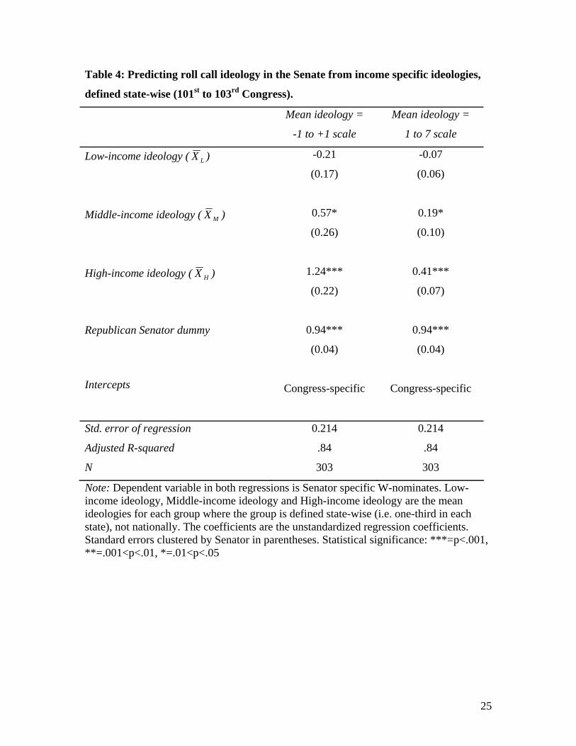
Table 4: Predicting roll call ideology in the Senate from income specific ideologies,

defined state-wise (101st to 103rd Congress).

Mean ideology =

-1 to +1 scale

Mean ideology =

1 to 7 scale

Low-income ideology ( LX )

Middle-income ideology ( MX )

High-income ideology ( HX )


-0.21

(0.17)

0.57*

(0.26)

1.24***

(0.22)

0.94***

(0.04)

Congress-specific

-0.07

(0.06)

0.19*

(0.10)

0.41***

(0.07)

0.94***

(0.04)

Congress-specific


Adjusted R-squared

N

0.214

.84

303

0.214

.84

303

Note: Dependent variable in both regressions is Senator specific W-nominates. Low-income ideology, Middle-income ideology and High-income ideology are the mean ideologies for each group where the group is defined state-wise (i.e. one-third in each state), not nationally. The coefficients are the unstandardized regression coefficients. Standard errors clustered by Senator in parentheses. Statistical significance: ***=p<.001, **=.001<p<.01, *=.01<p<.05

25

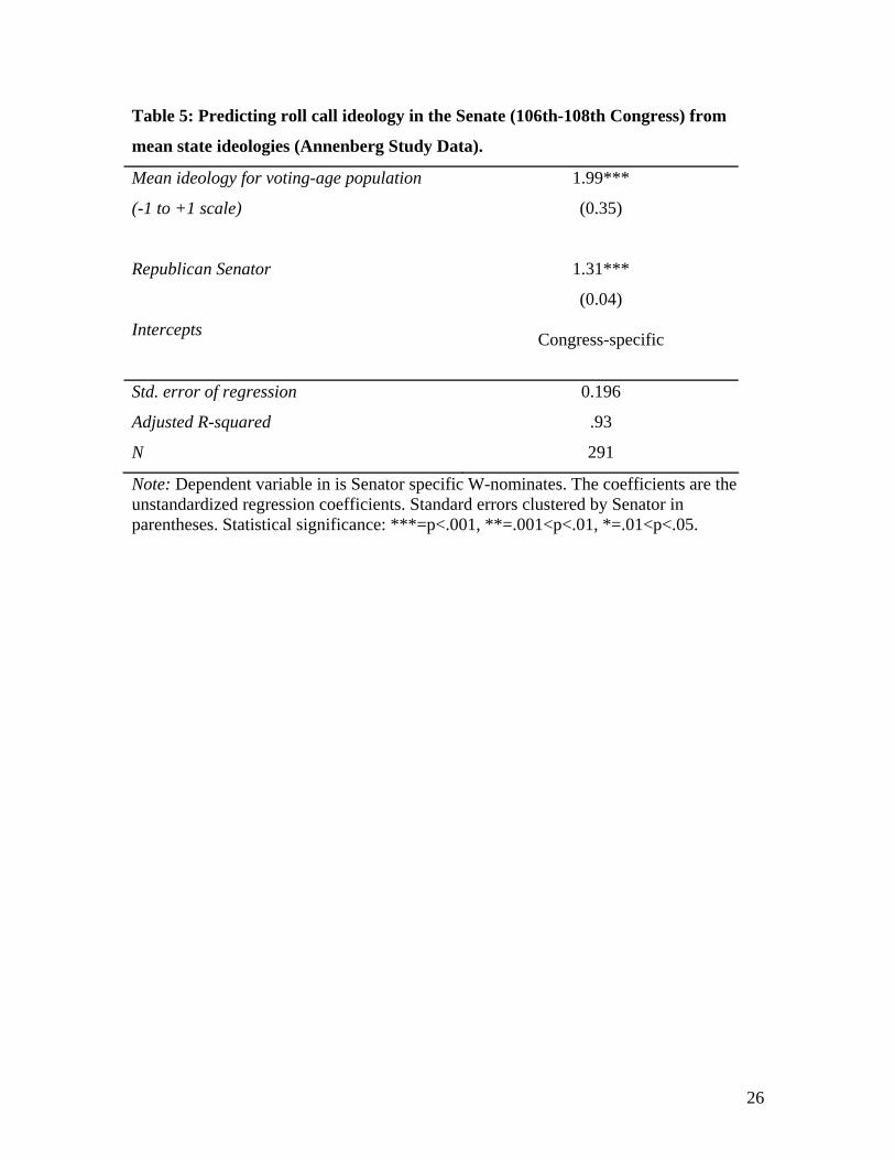
Table 5: Predicting roll call ideology in the Senate (106th-108th Congress) from

mean state ideologies (Annenberg Study Data).

Mean ideology for voting-age population

(-1 to +1 scale)

Republican Senator Intercepts

1.99***

(0.35)

1.31***

(0.04)

Congress-specific


Adjusted R-squared

N

0.196

.93

291

Note: Dependent variable in is Senator specific W-nominates. The coefficients are the unstandardized regression coefficients. Standard errors clustered by Senator in parentheses. Statistical significance: ***=p<.001, **=.001<p<.01, *=.01<p<.05.

26

Table 6: Predicting roll call ideology in the Senate (106th-108th Congress) from

income-specific ideologies, defined nationally (Annenberg Study data).

Mean ideology =

-1 to +1 scale







Intercepts

1.02

(1.14)

2.06

(1.99)

3.72*

(1.57)

1.30***

(0.05)

0.02

(0.79)

-0.56

(0.82)

Congress-specific


Adjusted R-squared

N

0.194

.93

291

Note: Dependent variable is Senator specific W-nominates. Wgt. low-income ideology, Wgt. middleincome-ideology and Wgt. high-income ideology are the raw mean ideologies for the respective income groups times the proportion of that group. The groups are defined nationally. Proportion low-income and Proportion high-income denotes the proportions entered separately. The coefficients are the unstandardized regression coefficients. Standard errors clustered by Senator in parentheses. Statistical significance: ***=p<.001, **=.001<p<.01, *=.01<p<.05.

27

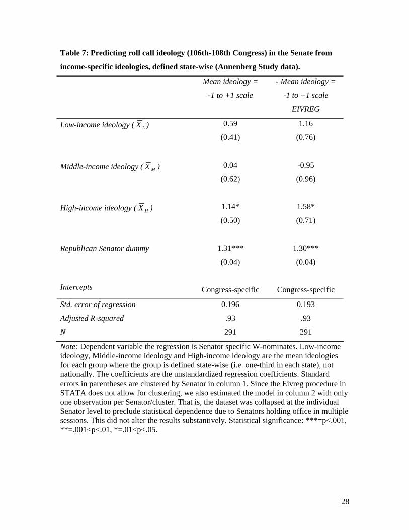
Table 7: Predicting roll call ideology (106th-108th Congress) in the Senate from

income-specific ideologies, defined state-wise (Annenberg Study data).

Mean ideology =

-1 to +1 scale

- Mean ideology =

-1 to +1 scale

EIVREG

Low-income ideology ( LX )

Middle-income ideology ( MX )

High-income ideology ( HX )


0.59

(0.41)

0.04

(0.62)

1.14*

(0.50)

1.31***

(0.04)

Congress-specific

1.16

(0.76)

-0.95

(0.96)

1.58*

(0.71)

1.30***

(0.04)

Congress-specific


Adjusted R-squared

N

0.196

.93

291

0.193

.93

291

Note: Dependent variable the regression is Senator specific W-nominates. Low-income ideology, Middle-income ideology and High-income ideology are the mean ideologies for each group where the group is defined state-wise (i.e. one-third in each state), not nationally. The coefficients are the unstandardized regression coefficients. Standard errors in parentheses are clustered by Senator in column 1. Since the Eivreg procedure in STATA does not allow for clustering, we also estimated the model in column 2 with only one observation per Senator/cluster. That is, the dataset was collapsed at the individual Senator level to preclude statistical dependence due to Senators holding office in multiple sessions. This did not alter the results substantively. Statistical significance: ***=p<.001, **=.001<p<.01, *=.01<p<.05.

28

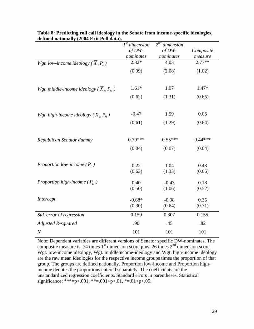
Table 8: Predicting roll call ideology in the Senate from income-specific ideologies, defined nationally (2004 Exit Poll data).

1st dimension of DW-

nominates

2nd dimension of DW-

nominates

Composite measure







Intercept

2.32*

(0.99)

1.61*

(0.62)

-0.47

(0.61)

0.79***

(0.04)

0.22 (0.63)

0.40

(0.50)

-0.68* (0.30)

4.03

(2.08)

1.07

(1.31)

1.59

(1.29)

-0.55***

(0.07)

1.04 (1.33)

-0.43 (1.06)

-0.08 (0.64)

2.77**

(1.02)

1.47*

(0.65)

0.06

(0.64)

0.44***

(0.04)

0.43 (0.66)

0.18

(0.52)

0.35 (0.71)


Adjusted R-squared

N

0.150

.90

101

0.307

.45

101

0.155

.82

101

Note: Dependent variables are different versions of Senator specific DW-nominates. The composite measure is .74 times 1st dimension score plus .26 times 2nd dimension score. Wgt. low-income ideology, Wgt. middleincome-ideology and Wgt. high-income ideology are the raw mean ideologies for the respective income groups times the proportion of that group. The groups are defined nationally. Proportion low-income and Proportion high-income denotes the proportions entered separately. The coefficients are the unstandardized regression coefficients. Standard errors in parentheses. Statistical significance: ***=p<.001, **=.001<p<.01, *=.01<p<.05.

29

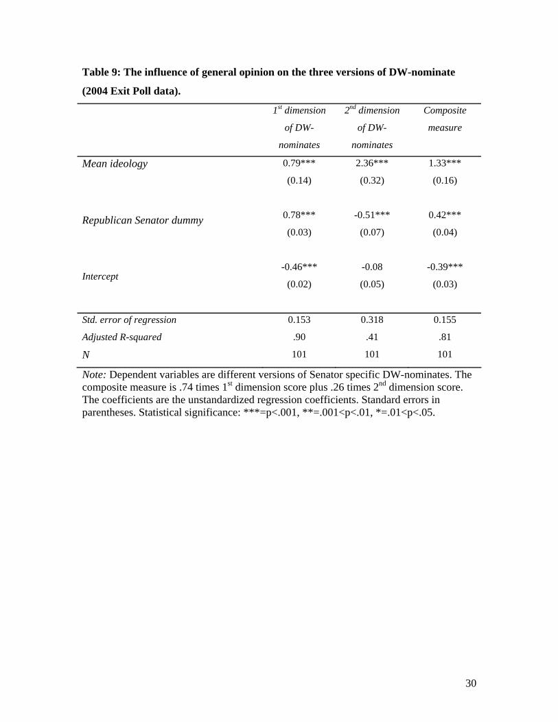
Table 9: The influence of general opinion on the three versions of DW-nominate

(2004 Exit Poll data).

1st dimension

of DW-

nominates

2nd dimension

of DW-

nominates

Composite

measure

Mean ideology


Intercept

0.79***

(0.14)

0.78***

(0.03)

-0.46***

(0.02)

2.36***

(0.32)

-0.51***

(0.07)

-0.08

(0.05)

1.33***

(0.16)

0.42***

(0.04)

-0.39***

(0.03)


Adjusted R-squared

N

0.153

.90

101

0.318

.41

101

0.155

.81

101

Note: Dependent variables are different versions of Senator specific DW-nominates. The composite measure is .74 times 1st dimension score plus .26 times 2nd dimension score. The coefficients are the unstandardized regression coefficients. Standard errors in parentheses. Statistical significance: ***=p<.001, **=.001<p<.01, *=.01<p<.05.

30

Table 10: Predicting Roll Call Ideology from Ideology of State Income Groups,

defined state-wise (2004 Exit Poll data).

1st dimension

of DW-

nominates

2nd dimension

of DW-

nominates

Composite

measure

Low-income ideology

Middle-income ideology

High-income ideology


Intercept

1.00

(0.86)

1.70

(1.04)

0.40

(0.76)

0.77***

(0.04)

-0.50***

(0.03)

-1.23

(1.79)

2.34

(2.17)

4.78**

(1.59)

-.60***

(0.07)

-0.12*

(0.06)

0.45

(0.89)

1.86

(1.08)

1.54

(0.79)

0.41***

(0.04)

-0.40***

(0.03)


Adjusted R-squared

N

0.149

.90

101

0.312

.44

101

0.155

.81

101

Note: Dependent variables are different versions of Senator specific DW-nominates. .The composite measure is .74 times 1st dimension score plus .26 times 2nd dimension score. Low-income ideology, Middle-income ideology and High-income ideology are the ideologies of voters in the state’s lowest, middle and highest third of family income respectively. The coefficients are the unstandardized regression coefficients. Standard errors in parentheses. Statistical significance: ***=p<.001, **=.001<p<.01, *=.01<p<.05.

31

Appendix – descriptive statistics and correlation matrices for the three surveys

For simplicity, all tables in the appendix are based on the -1- to +1 scale. The statistics

for the various decompositions of income groups are substantively very similar.

Table 11: Descriptive statistics for NES Senate study (-1 to +1 scale). Income groups

are defined nationally.

Variable Mean Std. dev. Min Max N

W-nominate 1st dimension -.19 0.54 -1.0 .99 303

Low-income ideology 0.14 0.11 -0.09 0.33 303

Middle-income ideology 0.15 0.09 -0.03 0.37 303

High-income ideology 0.13 0.09 -0.10 0.32 303

Overall mean ideology 0.14 0.07 0.03 0.31 303

Republican Senator .44 0.50 0 1 303

Table 12: Correlation matrix for NES Senate study (-1 to +1 scale). Income groups

are defined nationally.

WN LII MII HIO OMI RS

W-nominate 1st dimension (WN) -

Low-income ideology (LII) .01 -

Middle-income ideology (MII) .17 .31 -

High-income ideology (HIO) .31 .30 .33 -

Overall mean ideology (OMI) .23 .71 .78 .69 -

Republican Senator (RS) .89 -.04 .00 .09 .04 -

Note: The coefficients are the pair-wise correlations.

32

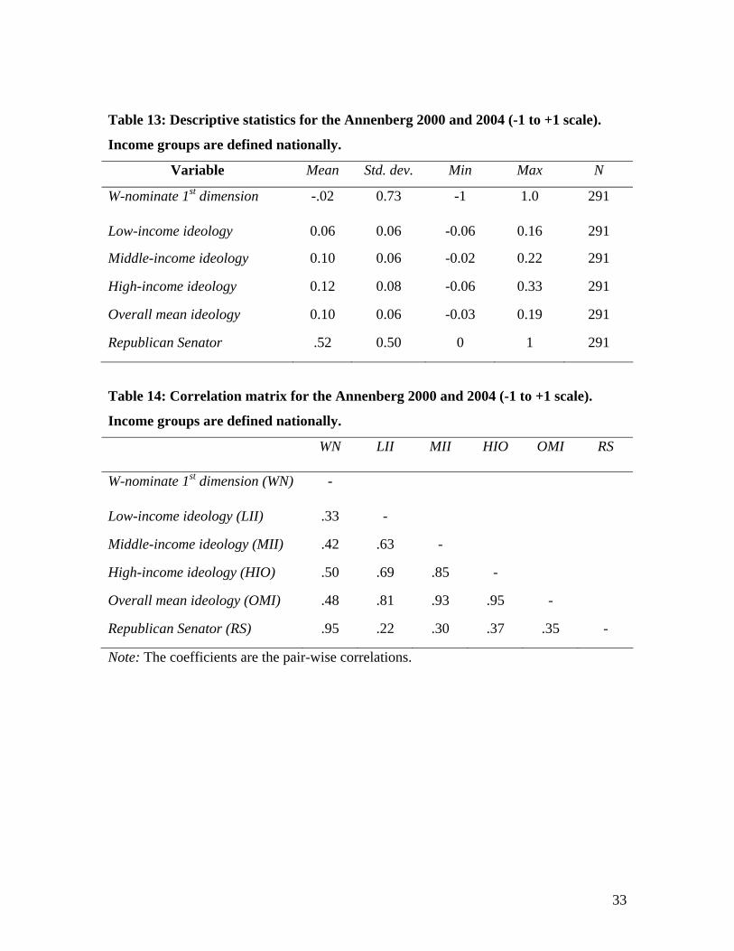
Table 13: Descriptive statistics for the Annenberg 2000 and 2004 (-1 to +1 scale).

Income groups are defined nationally.


W-nominate 1st dimension -.02 0.73 -1 1.0 291




Overall mean ideology 0.10 0.06 -0.03 0.19 291

Republican Senator .52 0.50 0 1 291

Table 14: Correlation matrix for the Annenberg 2000 and 2004 (-1 to +1 scale).

Income groups are defined nationally.


W-nominate 1st dimension (WN) -





Republican Senator (RS) .95 .22 .30 .37 .35 -


33

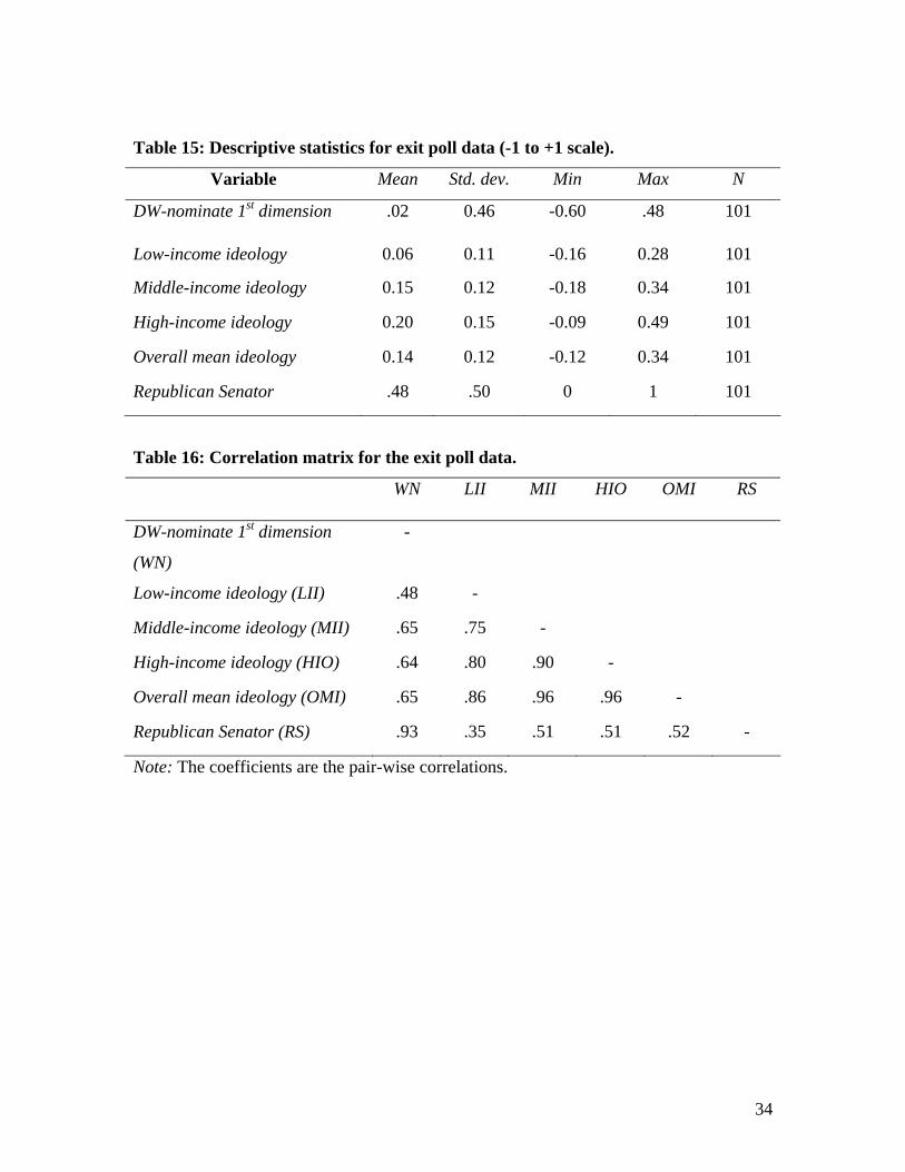
Table 15: Descriptive statistics for exit poll data (-1 to +1 scale).


DW-nominate 1st dimension .02 0.46 -0.60 .48 101




Overall mean ideology 0.14 0.12 -0.12 0.34 101

Republican Senator .48 .50 0 1 101

Table 16: Correlation matrix for the exit poll data.


DW-nominate 1st dimension

(WN)

-





Republican Senator (RS) .93 .35 .51 .51 .52 -


34

are rich and poor equally represented by lawmakers...

Documents