are agricultural land use patterns influenced by farmer imitation?

Are agricultural land use patterns influenced by farmer imitation?

Claude Schmit *, M.D.A. Rounsevell

Department of Geography, UCL, 3, Place Pasteur, 1348 Louvain-la-Neuve, Belgium

Received 11 April 2005; received in revised form 14 September 2005; accepted 28 December 2005

Available online 23 February 2006

Abstract

This paper proposes a methodology based solely on spatial data to analyse whether and, to what extent, farmer imitation leaves an

observable footprint on an agricultural landscape. Geographical Information System (GIS) analysis of parcel and farm location data of a study

region in central Belgium was developed as an alternative methodology to farmer interviews. Results suggest that imitation is not an important

determinant of agricultural land use patterns in the study area. The effect of imitation on landscapes is limited to the extent of being hardly

significant. Neighbouring parcels cultivated by farmers who live in close proximity are only slightly more similar than neighbouring parcels

cultivated by farmers who live further away from one another. The results question the validity of the assumptions underlying agent-based

models that try to explain agricultural land use through imitation behaviour.

The results should, however, be considered with caution as the proposed methodology has two limitations. First, comparison between

neighbouring parcels could not identify the imitation effect from all factors that influence agricultural land use. Relative space was not

accounted for, which led to two possible explanations for the similarity of neighbouring parcels: imitation or the location of a parcel relative to

the farm. Secondly, the method was applied to aggregated land use classes for a single year, which did not allow for the effect of crop rotations

in understanding imitation behaviour.

# 2006 Elsevier B.V. All rights reserved.

Keywords: Imitation; Agricultural land use; Farmer proximity; Agent-based model; Equi-finality

www.elsevier.com/locate/agee

Agriculture, Ecosystems and Environment 115 (2006) 113–127

1. Introduction

In modelling agricultural land use and land cover

distributions using an optimisation approach, Rounsevell

et al. (2003) generated patterns of land use that were more

spatially-distributed than the reality. They attributed this

observation to the influence of neighbouring land uses on

farmer choices (e.g. White and Engelen, 1993, 1997) that

were thought to create more concentrated land use patterns

in reality. This process can result in actual land use

distributions being significantly different from those, which

might be expected from a knowledge of the physical

conditions (soils and climates) and economic factors alone.

When making decisions about land use and management,

farmers have to cope with large uncertainties related to price

and cost fluctuations, weather variability and policy change.

* Corresponding author. Tel.: +32 10 47 85 06; fax: +32 10 47 28 77.

E-mail address: [email protected] (C. Schmit).

0167-8809/$ – see front matter # 2006 Elsevier B.V. All rights reserved.

doi:10.1016/j.agee.2005.12.019

Their behaviour is typified by multidimensional optimisa-

tion rather than a rational-actor-approach. When faced with

uncertainties, farmers seek robust solutions that often put

into play adaptive social processes (Festinger, 1954;

Lempert, 2002) such as imitation.

Farmers engage in imitation and repetitive behaviour

(habits) to efficiently use their limited cognitive resources

(Jager et al., 2000). Habits describe the repetition of their

originally deliberate choices for as long as the outcomes are

satisfying (Jager et al., 2000). Imitation is an automatic

social process, which relates to the theories of social

learning (Bandura, 1977, 1986) and normative conduct

(Cialdini et al., 1991). Social learning theory states that

watching another person being rewarded for understandable

and reproducible behaviour may result in the imitation of

that behaviour (Jager et al., 2000). Imitation has been

studied as part of the diffusion of innovation process (Ryan

and Gross, 1943; Hagerstrand, 1967). Adaptation of an

innovation depends on the characteristics of the innovation

C. Schmit, M.D.A. Rounsevell / Agriculture, Ecosystems and Environment 115 (2006) 113–127114

itself, the characteristics of the innovators (actors), and the

characteristics of the environmental context (Wejnert,

2002). Examples of farmer imitation behaviour include

the adoption of hybrid corn varieties (Ryan and Gross,

1943), conservation tillage practices (Warriner and Moul,

1992), new fertilizer (Feder and Umali, 1993) or grassland

management practices (Hagerstrand, 1967). Diffusion

processes strongly affect agriculture (Hagerstrand, 1967),

which suggests that private information and local social

networks are especially important in rural areas (Reimer,

1997; Hofferth and Iceland, 1998; Lindsay et al., 2005). The

exchange of information between individuals has been

found to be important for innovation decisions (Berger,

2001) and imitation is known to be a method that land

managers use in choosing between various options (Pomp

and Burger, 1995). Imitation can be understood as a strategy

to economise cognitive efforts, and/or to compensate for an

absence of knowledge (Jager et al., 2000). Imitation

strategies are based on the observation of successful land

uses or techniques (and conversely, avoidance of innovations

that are seen to fail). Farmers rely on information from past

decisions – their own and those of other agents – to update

decision-making strategies (Parker et al., 2002). At the most

critical stages in their decision process, farmers rely on

information brought to them by their peers (Berger, 2001).

Buttel et al. (1990) state that farmers’ decisions were

affected by the opinions and advice of neighbouring farmers.

Lowe et al. (1990) also found that farmers tend to give more

importance to sources of information that derive from the

farming community than elsewhere. The public nature of

farming favours farmer imitation strategies (Newby et al.,

1978). Farming is a very visible activity – visible, to other

local inhabitants, to anyone who passes through the

countryside and more importantly to other farmers.

The existence and observation of a neighbourhood effect

has led to the development of land use and land use change

models that integrate, implicitly, social and behavioural

factors into cellular automata (CA) and agent-based models

(ABM) (Verburg et al., 2004; Engelen et al., 2002; White and

Engelen, 1997; Berger, 2001; Batty et al., 1997; Caruso et al.,

2005). Most CA and ABM are, however, still theoretical. For

example, the Framework for the Evaluation and Assessment

of Regional Land Use Scenarios (FEARLUS) approach used a

simple, but abstract agent-based model to explore in a

spatially explicit way the performance of imitative versus

non-imitative strategies of land use selection by land

managers (Gotts et al., 2003). The model showed that the

success of a range of different imitative strategies depended

on the context in which imitation takes place. Performance

depends on the strategies being followed by other agents and

various aspects of the spatio-temporal heterogeneity of the

environment: the balance between spatial and temporal

variability, the predictability of variations over time, and the

scale of spatial heterogeneity (Polhill et al., 2001).

The incorporation of a micro-level perspective on human

behaviour within integrated models of land use and land

use change would potentially provide a better understanding

and eventual management of the processes involved in the

formation of landscape patterns (Jager et al., 2000).

However, a wide gap remains between the theoretical

implications of agent-based models (ABM) and empirical

data (Parker et al., 2003). It is difficult to parameterise and

validate ABM due to their large data requirements (Verburg

et al., 2001). A model of a complex land use system has

many parameters that change both in space and in time,

which require calibration and validation data at a high spatial

and temporal resolution. The lack of individual data limits

ABM model validation (Parker et al., 2003). Furthermore,

multi-agent models are often built on anecdotal evidence

because of the problem of equi-finality (or multi-causality)

that cannot always be resolved though calibration. The same

final state or condition of a system may be reached from

different initial conditions (inputs) and in different ways

(transformations). It is difficult to find unequivocal

empirical evidence for the very micro-level laws that give

the models their richness (Jager et al., 2000). With different

techniques, an infinite number of models can be created,

whilst reality remains constant. It is possible to develop a

model that can reproduce a statistically correct meta-

phenomenon with a model structure that does not capture

any real processes (Parker et al., 2003).

Taking advantage of the availability of detailed spatial

data, the research presented in this article addresses the

validity of the assumptions about imitation that underpin

many agent-based models of agricultural land use. More

generally, the objective of this paper was to propose a

methodology based solely on spatial data to analyze whether

and, to what extent, farmer imitation leaves an observable

footprint on land use in an agricultural landscape. The goal

was to gain insight into farmer imitation from the

Geographical Information System (GIS) analysis of parcel

and farm location data only. This is proposed as an

alternative (and complimentary) methodology to most

studies of social processes that use interviews or surveys

(Ryan and Gross, 1943; Stockdale, 2002; Chiffoleau, 2005;

Lindsay et al., 2005). The basic principle of the

methodology was to test whether the land use of

neighbouring parcels cultivated by farmers living close to

one another were more similar than neighbouring parcels of

farmers who are separated by greater distances. The

methodology relied on two assumptions. First, the socio-

informational networks of farmers decay with distance

(Ryan and Gross, 1943; Hagerstrand, 1967; Lindsay et al.,

2005). Thus, the distance between farms determines the

frequency of interactions and the quantity of information

exchanged between farmers. If imitation influences agri-

cultural land use patterns, then the distance between farms

cultivating two neighbouring parcels should influence the

similarity of those parcels. The second assumption was that

analysing neighbouring parcels allows the control of all

other factors (such as physical and political factors) that

influence agricultural land use. In comparing neighbouring

C. Schmit, M.D.A. Rounsevell / Agriculture, Ecosystems and Environment 115 (2006) 113–127 115

parcels over distances of a few hundred meters, it is

reasonable to assume that the independent variables of

climate, soils and policy (explaining the dependent variable

‘‘land use’’) are constant.

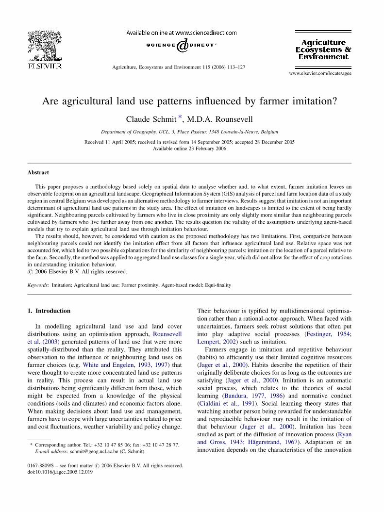
Fig. 1. Map of the location of the case study area (B, Brussels region).

2. Material and methods

2.1. The case study area

The work presented here is based on a case study region

in central Belgium defined as the Dyle river catchment

(508380N, 48450E) within the Walloon region, a 650 km2

catchment which is part of the Scheldt river basin. The study

region is characterised by a heterogeneous landscape that is

typical of northwest Europe, with a predominance of mixed

agriculture (crop cultivation and livestock production), and

high urbanisation (about 20% of the total land use area)

because of the proximity to Brussels. The study region was

chosen because detailed land use parcel data were available,

as well as additional spatial information.1

2.2. Parcel data

The basic landscape unit considered in this study is the

parcel, which is a contiguous entity of unique agricultural

land use cultivated by a single farmer. The vector land use

data used in this paper were obtained from the Integrated

Administration and Control System (IACS) (EEA, 2001).

The IACS monitor all agricultural parcels of holdings that

receive subsidies within the European Union (EU) area

payment scheme. Data is collected directly from farmers,

who are required to indicate the boundaries of all parcels

they cultivate on aerial photographs and to specify the land

use. These maps are digitised and used to monitor farmer

area declarations. The IACS vector dataset provides

therefore a detailed source of information about subsidised

agricultural land use (EEA, 2001) with high spatial detail

(parcel polygons) and thematic accuracy (more than 40

different crop types, see Appendix A).

The IACS database for the study region included all

parcels of farmers that cultivated at least one parcel within

the boundaries of the Dyle catchment during the year 1999.

Therefore, the extent of the dataset is not limited to the Dyle

catchment, as shown in Fig. 1. The dataset comprised 16,464

parcel polygons, of which 11,186 are located within the Dyle

catchment. The parcels cover an area of 48,660 ha (with

31,311 ha within the catchment). The main crop rotation is

winter wheat and sugar beet, which makes up half of the total

agricultural parcel area (winter wheat 30% and sugar beet

20%). Permanent grassland (16%) is the third most

important agricultural land use in terms of surface and

the second most important in terms of parcel numbers. The

1 Soil maps, climate data, road and river networks, administrative bound-

aries, aerial photography, agricultural census data per commune.

parcels are cultivated by 918 farm holdings, of which the

average farm size is 53 ha. The parcels are located in the

same administrative region, and therefore the same laws and

regulations apply.

2.3. Farm location data

The locations of farm buildings were manually geo-

coded as points. The farm building postal addresses were

collected for every farm holding cultivating at least one

parcel within the boundaries of the Dyle catchment. These

addresses were located on a map using an online route-

planning program (www.mappy.be). In ArcMap 8.3

(Environmental Systems Research Institute, ESRI Inc.),

the exact building locations were identified on aerial

photographs and digitised topographic maps at a scale of

1:10,000. For 67 of the 918 farms, postal addresses were

not available. For each of these farms, the gravity centre

of the farm’s parcels was calculated. The farm building

location was then estimated as the closest building

(recognizable on the 1:10,000 topographic map or on

the aerial photographs) to the gravity centre.

Some farmers operate from several production units

without declaring all of them, whereas others do not

necessarily cultivate their parcels from the location

specified in their mailing address. A field survey was used,

therefore, to validate a subset of the geocoded database.

Furthermore, an effort was made to quantify the uncertainty

or error associated with the location of all of the farm

buildings. A small sub-routine programmed in ArcMap

allowed the display of a particular farm location and its

corresponding parcels. Visual analysis of the mapped

representation of the farm building location relative to the

location of the parcels allowed an expert judgement to be

made about the quality of the geo-referenced farm

locations. A variable named ‘‘LOK’’ was generated for

each farm to quantify the subjective confidence in the

location of the farm buildings, based on criteria such as the

http://www.mappy.be/


Table 1

Coding of the accuracy of the geocoded farm building locations

Farm location OK? LOK-value

Perfect, no doubts 5

Good 4

Fair 3

Unusual, but possible 2

Bad, not likely 1

Worse 0

Missing �1

LOK-value, location of farm OK-value.

Fig. 2. Illustration of the buffer 50 m method to determine neighbouring

parcel pairs.

dispersion of the parcels relative to the farm, the distance

from the farm to the closest parcel and on the overall

clustering of the parcels. The ‘‘LOK’’ coding is shown in

Table 1.

The subsequent sections outline how the imitation

hypothesis was tested and describe how ‘‘neighbouring

parcels’’, ‘‘similarity’’ and ‘‘social distance’’ were deter-

mined.

2.4. Neighbouring parcels

Individual parcels were in vector format polygons (ESRI

shapefiles) that represent their actual shape and georefer-

enced position. GIS techniques were used to define the

neighbourhood of each parcel and to link neighbouring

parcel pairs. Two approaches to the estimation of neighbours

were tested: 50 m buffers and Thiessen polygons.

2.4.1. Buffer 50 m neighbourhood (Buf50 m)

A buffer of 50 m was generated around each parcel using

the ARC MAP Buffer Wizard. The newly created polygons

included the parcel and a buffer zone of 50 m around the

parcel. An identifier of the original parcel (‘‘PID’’) was

attributed to each of the ‘‘parcel + Buffer’’ polygons. The

theme of the ‘‘parcel + Buffer’’ was intersected with the

‘‘parcels-only’’ theme. This produced an attribute table with

two parcel IDs in each row, which were the IDs of the parcels

neighbouring each other. In order to map the parcel

neighbours, a line theme was created in ARC CATALOG

to link the centroids of the neighbouring parcels (Fig. 2).

If parcel A is a neighbour of parcel B, then parcel B is also

a neighbour of parcel A. For the analysis of neighbouring

parcels, the direction of the link is of no importance.

Because every pair-wise observation is represented twice

(parcel link A–B and parcel link B–A), the dataset was

filtered for the redundant (B–A parcel link) representations

of neighbouring parcel pairs.

The buffer distance was set to 50 m for two reasons. First,

parcels separated by a road should still be regarded as

neighbours and most roads (except some highways) are less

than 50 m wide. Secondly, wider buffer distances would

generate more neighbouring parcel pairs and a larger dataset

is better for statistical analyses. However, over greater

distances, the physical characteristics of the environment are

no longer constant, which contravenes the basic assumption

made here that neighbouring parcels should have basically

the same physical characteristics.

A drawback of the buffer method is that parcels that are

further apart than the buffer distance are considered to be

completely isolated. These parcels are systematically

excluded from the analysis, which influences the results.

Thus, in order to test the sensitivity of the results to the

choice of method, an alternative way of defining parcel

neighbourhoods, based on the use of Thiessen polygons, was

also applied.

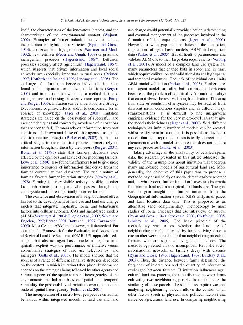
2.4.2. Thiessen polygon neighbourhoods

The parcels were first represented by a point theme that

was created from the coordinates of the centroids of the

parcel polygons. The Thiessen method creates non-over-

lapping polygons around each parcel centre point. Each

Thiessen polygon encloses the area that is the closest to the

enclosed parcel centre: the boundaries of the polygons are

fixed at an equal distance between two parcel centres.

Parcels were defined as neighbours if their respective

Thiessen polygons shared a common edge. The neighbour-

ing parcel pairs were linked with lines (Fig. 3).

The advantage of this method is that every parcel has a

similar number of neighbours and there are no isolated

parcels (compare Fig. 3 to Fig. 2). Conversely, the distance

between parcel neighbours can be highly variable.

2.5. Similarity

The similarity between neighbouring parcels was deter-

mined by agreement of the agricultural land use classes. Each

of the 43 different crops in the parcels dataset forms a

different agricultural land use class. For each neighbouring

parcel pair, a binary variable was created, which took the

value 1 if the land use of parcel Awas the same as the land use

of parcel B, and 0 otherwise. The ratio of similar parcel pairs


Fig. 3. Illustration of the Thiessen method to determine neighbouring

parcel pairs (for the same parcels as in Fig. 2).

2 A commune is the basic administrative unit in Belgium and is equivalent

to the NUTS 5 (Nomenclature of Territorial Units or Statistics) level.

Belgium is covered by a total of 589 communes.

over the total number of neighbouring parcel pairs (in

percent) was used as a general measure of similarity. Acreage

percentages were not considered because parcels, rather than

hectare, represent functional landscape units. Decisions

concerning land use are taken per parcel.

2.6. Social distance

If farmers follow imitation strategies they will gather

information from their peers. Due to a lack of spatial data on

social networks and social contacts, the exchange of

information between farmers was approximated, based on

indications from the literature. According to Lindsay et al.

(2005) social networks in rural areas tend to be small, dense

and homogeneous, confirming the findings of Hagerstrand

(1967): on average, the density of contacts included in a

single person’s private information field decreases very

rapidly with increasing distance. Social relationships within

rural communities have retained a distinctive culture and

dynamic (Halfacree, 1994). Despite life-style changes,

social networks provide stability (Letenyei, 2001; Harrison

and Carroll, 2002).

2.6.1. Neighbouring parcels cultivated by the same

farmer and by different farmers

The same farmer often cultivates neighbouring parcel

pairs. In this case the social distance is zero. The dataset of

unique neighbouring parcel pairs was split into two subsets:

parcel pairs cultivated by the same farmer, and parcel pairs

cultivated by different farmers. The frequencies of

neighbouring parcel pairs were summarised in a bivariate

table with the rows reporting whether farmers were the same

or different and the columns reporting whether parcels were

similar or not. A Chi-square (x2) test was carried out to

investigate the existence of a relationship between the two

variables (similarity of farms and similarity of neighbouring

parcels). Rejection of the null hypothesis indicates a

statistically significant relationship between the variables.

A significant relationship could be interpreted as a sign of

auto-imitation (Polhill et al., 2001), but this was not the main

objective of the work presented here. Subsequent analyses

were, therefore, performed on the subset of neighbouring

parcel pairs cultivated by different farmers.

2.6.2. Administrative units

A hierarchical system of administrative units may impose

a certain structure on human societies. In Belgium, the

hierarchical levels include communes,2 arrondissements,

provinces, regions and the nation state. As communes occur

at the lowest level in this hierarchical structure it was

hypothesised that farmers belonging to the same commune

would have more social contact than farmers belonging to

different communes. Social distance between farmers

cultivating neighbouring parcel pairs was, therefore, related

to the administrative units within which the farms were

located. For every neighbouring parcel pair, the farm

building locations of both parcels were joined to the parcel

link attribute table. Farm locations were given a commune

code based on the location of the farm building. The Dyle

catchment study area included 7 complete communes and

parts of a further 24 communes. The neighbouring parcels of

farmers living in the same commune were then compared to

neighbouring parcels of farmers living in different commu-

nes. In this way, the commune level was used to represent the

community where the farmer exchanges information.

Whether a farm pair was located in the same or in a different

administrative unit was coded with a binary variable. As

before, frequencies were summarised in a bivariate table

and a Chi-square test was used to analyse the relationship

between the similarity of neighbouring parcels and the

similarity of the communes of the farms cultivating those

parcels. Parcel pairs cultivated by farms located within the

same commune were expected to be more similar than those

cultivated by farms located within different communes.

2.6.3. Euclidian distance

The use of a binary variable (same or different commune)

masks information about the distance decay in social

networks. Exchange of information between farmers may be

stronger between administrative units that are closer to one

another than between those that are further apart. In order to

characterise the distance decay function in social networks

in greater detail a cardinal variable was calculated, the

Euclidian distance between farm buildings of parcels

located next to one another. The farm buildings of

neighbouring parcel pairs were linked by a line theme.

Then, the distances between farms were classified into

100 m intervals. Absolute and cumulated frequencies of the

neighbouring parcel pairs as a function of the distance


between farms were represented on a graph. Furthermore,

within each 100 m interval, the ratio of the frequency of

neighbouring parcel pairs to the same land use over the total

number of neighbouring parcel pairs was calculated accord-

ing to Eq. (1) and plotted on another graph representing

the similarity of neighbouring parcel pairs against distance

between farms.

Sið%Þ ¼Nsi100

N�i(1)

where Si(%) is the similarity (in percent) between neigh-

bouring parcel pairs for ‘‘distance between farms’’ interval i,

Nsi the number of neighbouring parcel pairs with the same

land use cultivated by farmers who live within a distance

interval i of one another, N�i is the total number of neigh-

bouring parcel pairs cultivated by farmers who live within a

distance interval i of one another.

The similarity values per 100 m farm distance intervals

were compared to the average similarity between neigh-

bouring parcels for the whole dataset (for all distances

between farms) in order to test whether parcels are more

similar when the farms cultivating them are closer to one

another. A polynomial trend was fitted to the points

representing the similarity versus distance between farms.

First, a second order polynomial was applied to the observed

points based on the equation:

Sið%Þ ¼ aþ b1distþ b2dist2 (2)

with dist expressed in metres. When the b2 coefficient in

Eq. (2) was not significant at the 0.05 threshold, the points

were approximated with a linear regression, characterised by

the following equation:

Sið%Þ ¼ aþ b1dist (3)

The sensitivity of the results to the choice of the method

for defining neighbouring parcels (Buf50 m or Thiessen

method) and to the uncertainty linked to the geocoding of

the farms were both investigated. In order to facilitate

comparison, similarity between neighbouring parcel pairs as

a function of distance between farms was expressed as a

location-specialisation index I1 (Eq. (4)).

I1 ¼Nsi=N�iN�s=N��

(4)

(adapted from Beguin, 1979); where Nsi is the number of

neighbouring parcel pairs with the same land use cultivated

by farmers who live within a distance interval i of one

another, N�i the total number of neighbouring parcel pairs

cultivated by farmers who live within a distance interval i of

one another, Ns� the total number of neighbouring parcel

pairs with the same land use (for all farm locations), and N��is the total number of neighbouring parcel pairs. The I1 index

compares the percentage of similar parcels within a ‘‘dis-

tance between farms’’ interval to the average percentage of

similar parcels in the study area. A value above 1 indicates

that similar parcel pairs are over-represented within a ‘‘dis-

tance between farms’’ interval.

In order to quantify the effect of the uncertainty associated

with the geocoding of farm locations on the similarity

between neighbouring parcels, the dataset of all parcel pairs

(determined with the Buf50 m method) was filtered according

to a threshold value of a new variable named MLOK. MLOK

was defined as the product of the LOK variable (see Table 1)

for both of the farms linked through a neighbouring parcel

pair. Threshold values were fixed at 9 and 15.

2.7. Exclusion of grassland

Previous studies on the same parcel database showed that

the location of grassland has a strong relationship with the

distance between parcels and farms (Schmit et al., 2006).

This may bias the conclusions about the possible influence

of farmer imitation on agricultural land use patterns.

Therefore, a further analysis was undertaken in which all

grassland parcels were excluded from the dataset of the

neighbouring parcel pairs cultivated by different farmers,

determined with the Buf50 m method. The effect of grass-

land exclusion on the similarity of parcel pairs was analysed

with the social distance measured both as the Euclidian

distance between farms and as the similarity of communes.

The use of this approach is further discussed later.

3. Results and discussion

In the following discussion, unless otherwise stated, the

Buf50 m method was used to determine neighbouring parcel

pairs. The results are presented from the most general to the

most detailed level of analysis.

3.1. Neighbouring parcels cultivated by the same

farmer and by different farmers

Thirty-seven thousand five hundred and thirty-six unique

neighbouring parcel pairs were determined (with the

Buf50 m method) from the 16,464 agricultural parcels in

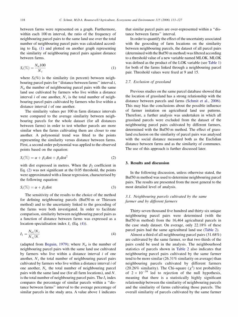
the case study dataset. On average, only 22.18% of these

parcel pairs had the same agricultural land use (Table 2).

Almost a third of all neighbouring parcel pairs (31.68%)

are cultivated by the same farmer, so that two thirds of the

pairs could be used in the analysis. The neighbourhood

statistics of parcels shown in Table 2 also indicates that

neighbouring parcel pairs cultivated by the same farmer

tend to be more similar (26.31% similarity on average) than

neighbouring parcels cultivated by different farmers

(20.26% similarity). The Chi-square (x2) test probability

of 2 � 10�39 led to rejection of the null hypothesis,

meaning that there is a statistically highly significant

relationship between the similarity of neighbouring parcels

and the similarity of farms cultivating those parcels. The

overall similarity of parcels cultivated by the same farmer


Table 2

The cross-tablulation matrix of the similarity of unique neighbouring parcel

pairs against the similarity of farms that cultivate neighbouring parcels

Farms Neighbouring parcel pairs land use

Different Same Total

Different 20449 5196 2564554.48 13.84 68.32

79.74 20.26 100.00

70.00 62.41 68.32

Same 8762 3129 1189123.34 8.34 31.68

73.69 26.31 100.00

30.00 37.59 31.68

Total 29211 8325 3753677.82 22.18 100.00

77.82 22.18 100.00

100.00 100.00 100.00

The upper numbers of each entry (in bold) give the absolute frequencies, the

second numbers (in normal font) give the percentages of all observations

(37,536), the third numbers (in italic) give the percentages of the row totals,

the fourth numbers (also in normal font) give the percentages of column

totals.

of 26.31% can be interpreted as a sign of mixed farming

(crops and livestock). On average one farmer cultivates 6

different crops. With specialized farms (farms cultivating a

single crop), the similarity between neighbouring parcel

pairs cultivated by the same farmer would be expected to be

much higher.

3.2. Administrative units

Table 3 shows the results of the comparison of the

neighbouring parcels of farmers living in the same commune

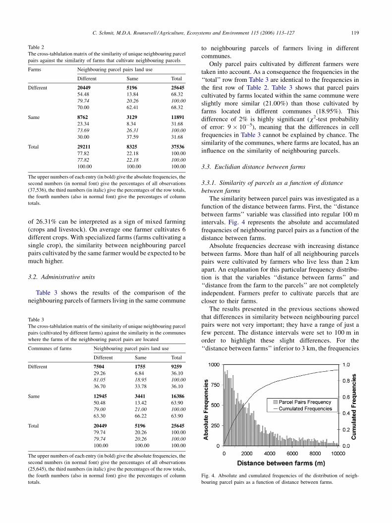
Table 3


pairs (cultivated by different farms) against the similarity in the communes

where the farms of the neighbouring parcel pairs are located

Communes of farms Neighbouring parcel pairs land use


Different 7504 1755 925929.26 6.84 36.10

81.05 18.95 100.00

36.70 33.78 36.10

Same 12945 3441 1638650.48 13.42 63.90

79.00 21.00 100.00

63.30 66.22 63.90

Total 20449 5196 2564579.74 20.26 100.00

79.74 20.26 100.00

100.00 100.00 100.00



(25,645), the third numbers (in italic) give the percentages of the row totals,

the fourth numbers (also in normal font) give the percentages of column

totals.

to neighbouring parcels of farmers living in different

communes.

Only parcel pairs cultivated by different farmers were

taken into account. As a consequence the frequencies in the

‘‘total’’ row from Table 3 are identical to the frequencies in

the first row of Table 2. Table 3 shows that parcel pairs

cultivated by farms located within the same commune were

slightly more similar (21.00%) than those cultivated by

farms located in different communes (18.95%). This

difference of 2% is highly significant (x2-test probability

of error: 9 � 10�5), meaning that the differences in cell

frequencies in Table 3 cannot be explained by chance. The

similarity of the communes, where farms are located, has an

influence on the similarity of neighbouring parcels.

3.3. Euclidian distance between farms

3.3.1. Similarity of parcels as a function of distance

between farms

The similarity between parcel pairs was investigated as a

function of the distance between farms. First, the ‘‘distance

between farms’’ variable was classified into regular 100 m

intervals. Fig. 4 represents the absolute and accumulated

frequencies of neighbouring parcel pairs as a function of the

distance between farms.

Absolute frequencies decrease with increasing distance

between farms. More than half of all neighbouring parcels

pairs were cultivated by farmers who live less than 2 km

apart. An explanation for this particular frequency distribu-

tion is that the variables ‘‘distance between farms’’ and

‘‘distance from the farm to the parcels’’ are not completely

independent. Farmers prefer to cultivate parcels that are

closer to their farms.

The results presented in the previous sections showed

that differences in similarity between neighbouring parcel

pairs were not very important; they have a range of just a

few percent. The distance intervals were set to 100 m in

order to highlight these slight differences. For the

‘‘distance between farms’’ inferior to 3 km, the frequencies

Fig. 4. Absolute and cumulated frequencies of the distribution of neigh-

bouring parcel pairs as a function of distance between farms.


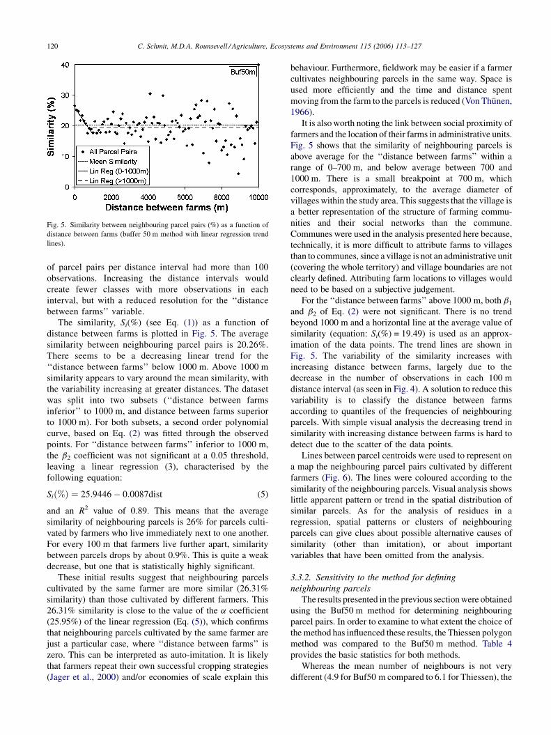
Fig. 5. Similarity between neighbouring parcel pairs (%) as a function of

distance between farms (buffer 50 m method with linear regression trend

lines).

of parcel pairs per distance interval had more than 100

observations. Increasing the distance intervals would

create fewer classes with more observations in each

interval, but with a reduced resolution for the ‘‘distance

between farms’’ variable.

The similarity, Si(%) (see Eq. (1)) as a function of

distance between farms is plotted in Fig. 5. The average

similarity between neighbouring parcel pairs is 20.26%.

There seems to be a decreasing linear trend for the

‘‘distance between farms’’ below 1000 m. Above 1000 m

similarity appears to vary around the mean similarity, with

the variability increasing at greater distances. The dataset

was split into two subsets (‘‘distance between farms

inferior’’ to 1000 m, and distance between farms superior

to 1000 m). For both subsets, a second order polynomial

curve, based on Eq. (2) was fitted through the observed

points. For ‘‘distance between farms’’ inferior to 1000 m,

the b2 coefficient was not significant at a 0.05 threshold,

leaving a linear regression (3), characterised by the

following equation:

Sið%Þ ¼ 25:9446� 0:0087dist (5)

and an R2 value of 0.89. This means that the average

similarity of neighbouring parcels is 26% for parcels culti-

vated by farmers who live immediately next to one another.

For every 100 m that farmers live further apart, similarity

between parcels drops by about 0.9%. This is quite a weak

decrease, but one that is statistically highly significant.

These initial results suggest that neighbouring parcels

cultivated by the same farmer are more similar (26.31%

similarity) than those cultivated by different farmers. This

26.31% similarity is close to the value of the a coefficient

(25.95%) of the linear regression (Eq. (5)), which confirms

that neighbouring parcels cultivated by the same farmer are

just a particular case, where ‘‘distance between farms’’ is

zero. This can be interpreted as auto-imitation. It is likely

that farmers repeat their own successful cropping strategies

(Jager et al., 2000) and/or economies of scale explain this

behaviour. Furthermore, fieldwork may be easier if a farmer

cultivates neighbouring parcels in the same way. Space is

used more efficiently and the time and distance spent

moving from the farm to the parcels is reduced (Von Thunen,

1966).

It is also worth noting the link between social proximity of

farmers and the location of their farms in administrative units.

Fig. 5 shows that the similarity of neighbouring parcels is

above average for the ‘‘distance between farms’’ within a

range of 0–700 m, and below average between 700 and

1000 m. There is a small breakpoint at 700 m, which

corresponds, approximately, to the average diameter of

villages within the study area. This suggests that the village is

a better representation of the structure of farming commu-

nities and their social networks than the commune.

Communes were used in the analysis presented here because,

technically, it is more difficult to attribute farms to villages

than to communes, since a village is not an administrative unit

(covering the whole territory) and village boundaries are not

clearly defined. Attributing farm locations to villages would

need to be based on a subjective judgement.

For the ‘‘distance between farms’’ above 1000 m, both b1

and b2 of Eq. (2) were not significant. There is no trend

beyond 1000 m and a horizontal line at the average value of

similarity (equation: Si(%) = 19.49) is used as an approx-

imation of the data points. The trend lines are shown in

Fig. 5. The variability of the similarity increases with

increasing distance between farms, largely due to the

decrease in the number of observations in each 100 m

distance interval (as seen in Fig. 4). A solution to reduce this

variability is to classify the distance between farms

according to quantiles of the frequencies of neighbouring

parcels. With simple visual analysis the decreasing trend in

similarity with increasing distance between farms is hard to

detect due to the scatter of the data points.

Lines between parcel centroids were used to represent on

a map the neighbouring parcel pairs cultivated by different

farmers (Fig. 6). The lines were coloured according to the

similarity of the neighbouring parcels. Visual analysis shows

little apparent pattern or trend in the spatial distribution of

similar parcels. As for the analysis of residues in a

regression, spatial patterns or clusters of neighbouring

parcels can give clues about possible alternative causes of

similarity (other than imitation), or about important

variables that have been omitted from the analysis.

3.3.2. Sensitivity to the method for defining

neighbouring parcels

The results presented in the previous section were obtained

using the Buf50 m method for determining neighbouring

parcel pairs. In order to examine to what extent the choice of

the method has influenced these results, the Thiessen polygon

method was compared to the Buf50 m method. Table 4

provides the basic statistics for both methods.

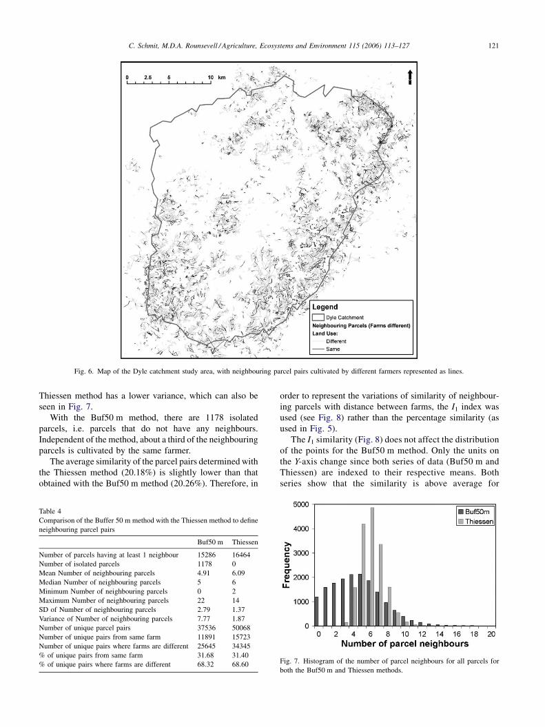
Whereas the mean number of neighbours is not very

different (4.9 for Buf50 m compared to 6.1 for Thiessen), the


Fig. 6. Map of the Dyle catchment study area, with neighbouring parcel pairs cultivated by different farmers represented as lines.

Thiessen method has a lower variance, which can also be

seen in Fig. 7.

With the Buf50 m method, there are 1178 isolated

parcels, i.e. parcels that do not have any neighbours.

Independent of the method, about a third of the neighbouring

parcels is cultivated by the same farmer.

The average similarity of the parcel pairs determined with

the Thiessen method (20.18%) is slightly lower than that

obtained with the Buf50 m method (20.26%). Therefore, in

Table 4

Comparison of the Buffer 50 m method with the Thiessen method to define

neighbouring parcel pairs

Buf50 m Thiessen

Number of parcels having at least 1 neighbour 15286 16464

Number of isolated parcels 1178 0

Mean Number of neighbouring parcels 4.91 6.09

Median Number of neighbouring parcels 5 6

Minimum Number of neighbouring parcels 0 2

Maximum Number of neighbouring parcels 22 14

SD of Number of neighbouring parcels 2.79 1.37

Variance of Number of neighbouring parcels 7.77 1.87

Number of unique parcel pairs 37536 50068

Number of unique pairs from same farm 11891 15723

Number of unique pairs where farms are different 25645 34345

% of unique pairs from same farm 31.68 31.40

% of unique pairs where farms are different 68.32 68.60

order to represent the variations of similarity of neighbour-

ing parcels with distance between farms, the I1 index was

used (see Fig. 8) rather than the percentage similarity (as

used in Fig. 5).

The I1 similarity (Fig. 8) does not affect the distribution

of the points for the Buf50 m method. Only the units on

the Y-axis change since both series of data (Buf50 m and

Thiessen) are indexed to their respective means. Both

series show that the similarity is above average for

Fig. 7. Histogram of the number of parcel neighbours for all parcels for

both the Buf50 m and Thiessen methods.


Fig. 8. Similarity between neighbouring parcel pairs (expressed as the I1

index) as a function of distance between farms, Thiessen method compared

to Buf50 m method.


index) as a function of distance between farms, according to the different

levels of certainty associated to the geocoded farm locations.

Table 5

Summary of the coefficients of the linear regressions for ‘‘distance between

farms’’ inferior to 1000 m

Method Subset a b1 R2

Buf50 m All 1.2805*** �0.00043*** 0.89

Thiessen All 1.1640*** �0.00019* 0.52

Buf50 m MLOK � 9 1.3155*** �0.00051*** 0.86

Buf50 m MLOK � 15 1.3378*** �0.00057*** 0.87

Buf50 m Grass Excl. 1.1399*** �0.00023* 0.37

Buf50 m Grass Excl.

and Dff > 0

1.1144*** �0.00018 0.32

Significance of the coefficients is marked with stars: *** = P < 0.001;** = P < 0.01; * = P < 0.05. For the subset variable: all = all neighbouring

parcel pairs cultivated by different farmers; Dff > 0 = ‘‘distance between

farms’’ is strictly greater than zero metres.

‘‘distance between farms’’ inferior to 700 m. For the

‘‘distance between farms’’ inferior to 1000 m, the linear

trend for the Buf50 m method was characterised by the

equation Si(I1) = 1.2805 � 0.0004dist, with an R2 value of

0.89, whereas for the Thiessen method, the trend was

defined by Si(I1) = 1.1640 � 0.0002dist, with an R2 value

of 0.52. Both the a and b1 coefficients and the R2 value were

lower for the Thiessen method than for the Buf50 m

method. The linearly decreasing trend with increasing

distance between farms is not as well defined for the

Thiessen method as for the Buf50 m method. Overall, the

Thiessen points show a higher variability than the Buf50 m

points (Fig. 8). Nevertheless there is still a trend, with an

above average similarity for neighbouring parcels culti-

vated by farmers who live close to one another.

3.3.3. Uncertainty linked to the geocoding of the farms

The subsets MLOK � 9 and MLOK � 15 are subsets

of the neighbouring parcel pairs based on a judgement of

the uncertainty of the method used to georeference the

farm locations. MLOK � 9 means that the farms of both

parcels have at least a fair location (LOK variable value of

3) or one farm has a strange location (LOK = 2) and the

other one is geocoded perfectly (LOK = 5) (refer to

Table 1). Filtering the neighbouring parcel pairs according

to MLOK � 15 reduces the size of the dataset, but only

neighbouring parcel pairs are used for which the

uncertainty associated with the geocoding of farm loca-

tions is very low.

The two subsets are compared with the whole dataset in

Fig. 9. A similar trend in the first 1000 m ‘‘distance between

farms’’ can be observed for the three data series. Linear

regression on the ‘‘MLOK � 9’’ subset for the ‘‘distance

between farms’’ inferior to 1000 m gave the equation

Si(I1) = 1.3155 � 0.0005dist, with an R2 value of 0.86. The

‘‘MLOK � 15’’ subset resulted in the equation Si(I1) =

1.3378 � 0.0006dist with an R2 value of 0.87. The increased

certainty in the geocoding of the farm locations results in

increased similarity between neighbouring parcel pairs for

farms that are very close to one another (‘‘distance between

farms’’ < 100 m) and it amplifies the slope of the linear

trend within the first 1000 m ‘‘distance between farms’’ (a

and b1 coefficients of Eq. (3)). Filtering the data according to

the confidence in farm location emphasized the general trend

observed in the complete database, but does not change the

basic conclusions from the previous analyses.

Table 5 compares the linear trend adjusted through the

similarity points for the ‘‘distance between farms’’ inferior

to 1000 m. Independent of the method chosen, the trend

shows that parcels of farmers who live close to one another

are more similar than parcels of farmers who live further

apart. The linear trend is clearest for the Buf50 m method for

all neighbouring parcel pairs (highest R2 value). The

Thiessen method gives a much lower intercept (a) and

slope (b1), due to the fact that the distance between

neighbouring parcels is more variable for the Thiessen

method than for the Buf50 m method. Excluding parcels of

farms with an uncertain geocoded farm location results in a


Table 6


pairs (cultivated by different farms; grassland parcels excluded) vs. the

similarity in the communes where the farms of the neighbouring parcel pairs

are located

Communes

of farms

Neighbouring parcel pairs land use (grassland excl.)


Different 6038 1472 751029.94 7.30 37.24

80.40 19.60 100.00

37.63 35.73 37.24

Same 10007 2648 1265549.63 13.13 62.76

79.08 20.92 100.00

62.37 64.27 62.76

Total 16045 4120 2016579.57 20.43 100.00

79.57 20.43 100.00

100.00 100.00 100.00



(20,165), the third numbers (in italic) give the percentages of the row totals, the

fourth numbers (also in normal font) give the percentages of column totals.

higher intercept and slope because parcels of farms left in the

dataset are more clustered around the farm buildings.

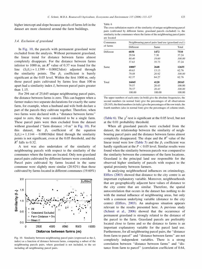
3.4. Exclusion of grassland

In Fig. 10, the parcels with permanent grassland were

excluded from the analysis. Without permanent grassland,

the linear trend for distance between farms almost

completely disappears. For the distance between farms

inferior to 1000 m, an R2 value of 0.37 was found for the

line (Si(I1) = 1.1399 � 0.00023dist) adjusted through

the similarity points. The b1 coefficient is barely

significant at the 0.05 level. Within the first 1000 m, only

those parcel pairs cultivated by farms less than 100 m

apart had a similarity index I1 between parcel pairs greater

than 1.15.

For 294 out of 25,645 unique neighbouring parcel pairs,

the distance between farms is zero. This can happen when a

farmer makes two separate declarations for exactly the same

farm, for example, when a husband and wife both declare a

part of the parcels they cultivate together. Therefore, when

two farms were declared with a ‘‘distance between farms’’

equal to zero, they were considered to be a single farm.

These parcel pairs were then excluded from the dataset

without grassland (‘‘farm distance >0 m’’ in Fig. 10). For

this dataset, the b1 coefficient of the equation

Si(I1) = 1.1144 � 0.00018dist fitted through the similarity

points is not significant, even at the 0.05 threshold, and the

R2 falls to 0.32.

A test was also undertaken of the similarity of

neighbouring parcels with respect to the similarity of the

communes where the farms are located. Only non-grassland

parcel pairs cultivated by different farmers were considered.

Parcel pairs cultivated by farms located in the same

commune were slightly more similar (20.92%) than those

cultivated by farms located in different communes (19.60%)


index) as a function of distance between farms, comparing a subset of the

neighbouring parcels pairs, where grassland is not included, to the set

including all neighbouring parcel pairs.

(Table 6). The x2-test is significant at the 0.05 level, but not

at the 0.01 probability threshold.

When all grassland parcels were excluded from the

dataset, the relationship between the similarity of neigh-

bouring parcel pairs and the distance between farms almost

completely disappeared. The slope and the R2 value of the

linear trend were low (Table 5) and the b1 coefficient was

hardly significant at the P < 0.05 level. Similar results were

found when the similarity between parcels was compared to

the similarity between the communes of the farm locations.

Grassland is the principal land use responsible for the

observed higher similarity of parcels with respect to the

spatial proximity between farmers.

In analysing neighbourhood influences on criminology,

Elffers (2003) showed that distance to the city centre is an

important explanatory variable. Moreover, neighbourhoods

that are geographically adjacent have values of distance to

the city centre that are similar. Therefore, the spatial

autocorrelation that occurs in the dataset has nothing to do

with the mutual influence of neighbouring areas, but only

with a common underlying variable (distance to the city

centre) (Elffers, 2003). An analogous situation appears

relevant to the results presented here. A previous study

(Schmit et al., 2006) showed that the occurrence of

permanent grassland is strongly related to the distance of

the parcel to the farm. Grassland parcels are preferably

located close to farms and so the distance to farms is an

important explanatory variable for the parcel land use.

Furthermore, for all neighbouring parcel pairs, the ‘‘distance

from farm to parcel’’ and ‘‘distance between farms’’ are not

completely independent variables. There is a strong

correlation between ‘‘distance between farms’’ and ‘‘dis-

tance from farm to parcel’’ (correlation coefficient of 0.64,


3 For example, climate varies very little across the study area, and the

differences must be minimal between adjacent parcels.

significant at P < 0.001). Thus, for two neighbouring

parcels of grassland, there is a high probability that the

farms owning these parcels are located in close proximity to

them. As a consequence there is a high chance that the farms

cultivating these neighbouring parcels are also close to one

another. By comparing neighbouring parcel pairs, it was

possible to control for the variability in the biophysical

space, but not for the variables related to relative space (i.e.

the distance of the parcels relative to the farm). Farm

location itself becomes an important determinant of

agricultural landscape structure.

Thus, there are two possible processes that can explain

the observed land use pattern. Neighbouring grassland

parcels are more similar than other crops either because

farmers imitate one another or because parcels are located

close to the farm and farmers prefer these parcels to be in

grassland. Based on Schmit et al. (2006), the second option

seems to be more likely and the analysis presented here does

not support the case for imitation.

This is a case of equi-finality, which probably results

from the hierarchy of processes that affect land use decision-

making. Purely physical factors determine the potential land

use space. Climate, soils and topography limit the number of

choices a farmer has concerning the land use on a particular

parcel. Economic factors then influence the exact choice of

land use, usually within the objective of maximising profit

and minimising risk (Rounsevell et al., 2003).

It appears that imitation does not affect land use patterns

directly. However, imitation of neighbouring farmers’

management options concerning land use may be a way

of confirming previously taken decisions about land use. A

farmer, facing alternative choices of land use that are

possible, economically profitable, equivalent in terms of

environmental impacts (sustainable development), might

therefore imitate neighbouring farmers to choose between

two options, that are similar form an economic perspective.

Both of these imitation processes could explain the

observation of slight similarity between parcels, but

imitation is not the major driver of agricultural land use

patterns in the study region.

3.5. Limitations of the method

3.5.1. Neighbouring parcels

The Buf50 m method to determine neighbouring parcel

pairs performed better than the Thiessen method. For the

Thiessen method, the distance between neighbouring

parcels was more variable and could be very large. Isolated

parcels were linked to the closest neighbouring parcels,

parcels that are sometimes several kilometres away. Over

larger distances, the physical characteristics of the

environment can no longer be considered to be identical,

which was an implicit assumption in the parcel comparison

methodology.

With the Buf50 m method it is reasonable to assume

that the physical characteristics of neighbouring parcels are

very similar,3 although this does not completely exclude the

possibility that the physical characteristics may vary

between adjacent parcel pairs. Soils, for example, are not

homogeneous over the study area and may be different

between adjacent parcels, modifying a farmer’s crop

choices. In the least favourable areas, parcels may be more

similar because the physical environment restricts crop

growth to a single crop, e.g.: grassland on wet soils in valley

bottoms (Souchere et al., 2003).

An alternative method for defining neighbouring parcels,

based on raster neighbourhoods was not taken into account,

even though the majority of land use change studies, as well

as most cellular automata and agent-based models work with

land use data in raster format (for examples, see Engelen

et al., 2002; Berger, 2001; Batty et al., 1997; Veldkamp and

Fresno, 1996). Raster data were not, however, used in this

study as they have a number of important limitations.

Technically, defining the neighbourhood of a raster cell is

straightforward, using either a Von Neumann (4 adjacent

cells) or a Moore neighbourhood (8 adjacent cells), or even

larger neighbourhoods, e.g. 196 cell neighbourhoods were

used in the Murbandy and Moland –CA’s (Engelen et al.,

2002). Depending on the raster resolution, however, large

parcels may be divided into several grid cells, or smaller

parcels may not be represented at all and the boundaries of

individual parcels cannot be distinguished. Raster cells do

not correspond to any functional unit in reality; farmers

make land use decisions with respect to parcels and not for

grid cells. Moreover, agricultural parcels differ in size. For

statistical analyses, working with a raster dataset at a

resolution lower than the parcel size increases the number of

observations, which leads to an overestimation of the

neighbourhood effect (due to spatial autocorrelation).

Furthermore, alternative raster representations alter the

composition and/or structure of the landscape (Schmit et al.,

2006). This implies that CA and/or ABM based on raster

data are not appropriate for studying the effects of imitation

on agricultural land use patterns.

If, as presented here, the role of imitation is hardly

significant for vector data, it seems optimistic to hope that

raster data would be any better at representing farmer

imitation. Moreover, it is possible that the commonly

observed neighbourhood effect is a function of the raster

data representation rather than reflecting any inherent

processes. This has important implications for neighbour-

hood-based agricultural land use change models.

3.5.2. Similarity

The dataset used in this study distinguished between 43

different agricultural land use classes. The number of classes

considered has an impact on the similarity between

neighbouring parcels. The larger the number of classes,

the lower the random probability of having two neighbour-


ing parcels that belong to the same class.4 Also, the 43

crop classes used here would probably be too numerous for

land use modelling purposes. However, 12 crops make up

90% of all parcels (see Appendix A). Minor crops were not

excluded from the analysis because often it is these minor

crops that are a clear sign of farmer imitation through the

process of innovation diffusion (Ryan and Gross, 1943;

Hagerstrand, 1967). The results of the imitation analysis

would not have varied greatly with the use of only the 12

most common crops.

A major limitation of the method is that similarity was

based on crops rather than on crop rotations. Attempts at

regrouping crops according to their rotations were unsuc-

cessful because of the large number of possible crop

rotations. In the study area, crop rotations commonly have a

periodicity of 3–5 years with sugar beet, maize or chicory in

the first year, followed by winter wheat in the second year

and winter barley, potatoes, fallow, flax or peas in the third

year. However, in addition to this several further possibilities

exist. Crops such as maize may be used in mono-culture as

well as in rotation. Multi-annual parcel data might allow a

‘‘sugar beet–winter wheat–potato’’ rotation to be separated

from a ‘‘chicory–winter wheat–flax’’ rotation, but this would

still not be straightforward as several crops are grown in

several different rotations. It is, however, at all possible with

data for a single year. Because of the diversity and

complexity of rotations, the results of this analysis should

be considered with great care. The method, however,

remains an appropriate means of gaining insight into

agricultural land use patterns that is applicable beyond the

study area presented here.

3.5.3. Social distance

Socio-informational networks of farmers are not neces-

sarily best characterised by the Euclidian distance between

farm locations or the farm location within an administrative

unit. A growing body of literature argues that traditional

family and social networks are less significant in today’s

society as a whole (Beck, 1992; Giddens, 1991; Hutton and

Giddens, 2000). Information transmission is not limited to

communication within a network of colleagues, but also

includes the media, farmers’ associations and public and

private advisory services. Furthermore, modern commu-

nication technologies (internet, telephone) have reduced

functional distance. As a consequence, the level of social

interaction may not decrease with increasing distance

between farms.

A fundamental principle of human communication is that

the transfer of ideas occurs most frequently between

individuals who have similar social profiles in terms of

attributes, beliefs, education, social status and the like

(Rogers, 1983). Applied to farmers, this would suggest a

4 For example, in a landscape composed of parcels of only two agricul-

tural land use classes, each covering half of the study area, spatially-

distributed at random, the similarity between neighbouring parcels is likely

to be around 50%.

higher probability of interaction between individuals with

similar farm typologies. It is possible that a potentially

imitating farmer would assess how far a ‘‘model’’ farmer’s

situation is similar to his own and, hence, how useful

imitation would be (Polhill et al., 2001). A farmer

specialised in field cropping is more likely to imitate a

farmer with the same typology rather than someone

specialised in livestock grazing. Family links and the level

of education are also likely to influence the social network of

the farmer. An attempt was made here to classify farms into

different typologies, based on the land use of the parcels.

Without additional socio-economic data, however, no clear

farm typologies could be distinguished, and the farm types

identified were greatly dependent on the choice of the

classification method.

3.5.4. Temporal dimension

The current analysis was based on a spatial snapshot of

the study region and the temporal dimension was not

taken into account. Imitation of neighbours is a process

that unfolds in both time and in space. The ‘‘temporal

footprint’’5 of farmer imitation on agricultural landscapes

may be more important than the ‘‘spatial footprint’’. The

analysis presented here was limited to a particular region

and to a particular moment in time. A landscape in

transition could reveal a spatial footprint of imitation on

land use patterns that is more important. Moreover, the

agricultural landscape of the Dyle catchment has been

stable in recent years (Schmit et al., 2006). In the future,

policy and climate change may force farmers to adapt

their land use to new conditions. During these transition

phases, the role of farmer imitation may become more

important.

4. Conclusion

The work reported here has attempted to answer the

question, to what extent does farmer imitation leave an

observable footprint on agricultural landscapes? An alter-

native method not based on farmer interviews, but on spatial

parcel and farm location data showed considerable potential

in addressing this question, but also some important

limitations. Results of the newly developed methodology

suggest that imitation is not an important determinant of

agricultural land use patterns in the Dyle Catchment.

Independent of the method or the subset used, the analysis

showed that neighbouring parcels cultivated by farmers who

live close to one another are very slightly more similar than

neighbouring parcels cultivated by farmers who live further

apart. The opposite trend was not observed. The main crop

responsible for the observed trend was grassland. Grassland

has a spatial distribution that is characterised by its relative

5 The term ‘‘temporal footprint’’ refers to the timing of land use change,

for example to ‘‘when’’ farmers first adopt new crops.


location with respect to a farm arising from accessibility

considerations by farmers rather than imitation. Results

suggest that including social behaviour in physical and

economic models of land use change would not, therefore,

add much to the explanation of observed land use patterns in

this region and for this moment in time.

The results of the analysis need, however, to be

considered with caution because of the limitations of the

proposed methodology. Comparison of neighbouring par-

cels did not allow all factors to be controlled that influence

agricultural land use, such as the distance of parcels to farm

for example. Further analysis and understanding of the

drivers of agricultural land use decisions may help to isolate

the effect of imitation. Another limitation of the method was

that similarity was defined using crop classes rather than

crop rotations. It might be possible to use multi-annual

parcel data to overcome this problem, so that crop rotations

can be identified, but such an approach would not be

straightforward given that the same crop can occur in several

different rotations.

This article presents, therefore, a methodology based on

observed land use data that is an alternative to social survey

based studies of farmer behaviour. The approach seeks to

apply hard methodologies to soft sciences, and may

contribute to the further development of cellular automata

and agent-based land use change models. For this purpose,

the analysis of time series of the same landscape is

preferable, in order to gain insight not only into the spatial,

but also into the temporal dimension of the effects of farmer

imitation on agricultural landscapes.

Acknowledgements

The authors wish to thank first the EU ACCELERATES

project (contract no. EVK2-CT2000-00061) and the

Luxembourg Ministry of Culture, Higher Education and

Research for funding this research, and the Direction

General de l’Agriculture (DGA) of the Walloon Region in

Belgium for the IACS parcel data and farm addresses.

Specifically, thanks are extended to Mr. Mokadem of the

Ministry of Agriculture for the description of available

datasets in the Walloon region and Mr. Dautrebande of the

Centre de Recherche Agronomique (CRA) of Gembloux

for supplying samples of IACS data for Belgium. The

authors would also like to acknowledge the contribution of

Dr. Isabelle La Jeunesse in the creation of the GIS database

and Mr. Thomas Crepin for his help in the geocoding

process.

Appendix A

Table with number of parcels, percentage of all parcels

and cumulated percentage of all parcels, for all land use

classes present in the Dyle Catchment

Rank
Land use (crop) Parcels Percentage Cumulated
percentage

1
Winter wheat 3809 23.14 23.14
2
Permanent grassland 3136 19.05 42.18
3
Sugar beet 2342 14.22 56.41
4
Silage maize 1876 11.39 67.80
5
Winter barley 830 5.04 72.84
6
Fallow (grains) 594 3.61 76.45
7
Potatoes 512 3.11 79.56
8
Fallow (grains and pulses) 493 2.99 82.56
9
Non-permanent grassland 435 2.64 85.20
10
Chicory 397 2.41 87.61
11
Spring barley 265 1.61 89.22
12
Grain maize 229 1.39 90.61
13
Fallow (natural cover) 166 1.01 91.62
14
Other fallow 145 0.88 92.50
15
Oats 138 0.84 93.34
16
Spring wheat 107 0.65 93.99
17
Other (tobacco, hops, . . .) 107 0.65 94.64
18
Flax 99 0.60 95.24
19
Peas 88 0.53 95.77
20
Mixed fallow 78 0.47 96.25
21
Forage beet 75 0.46 96.70
22
Other fodder 72 0.44 97.14
23
Pulses 67 0.41 97.55
24
Market gardening 67 0.41 97.95
25
German wheat 56 0.34 98.29
26
Field beans 56 0.34 98.63
27
Dried peas 45 0.27 98.91
28
Triticale 43 0.26 99.17
29
Oilseed rape (winter) 43 0.26 99.43
30
Winter oilseed rape 35 0.21 99.64
31
Non-food horticulture 11 0.07 99.71
32
Fruit crops 11 0.07 99.78
33
Lucerne 10 0.06 99.84
34
Dried beans 8 0.05 99.88
35
Beans 6 0.04 99.92
36
Other grains 3 0.02 99.94
37
Clover 3 0.02 99.96
38
Wood 2 0.01 99.97
39
Oilseed rape (spring) 1 0.01 99.98
40
Sunflower 1 0.01 99.98
41
Linseed 1 0.01 99.99
42
Fodder carrot 1 0.01 99.99
43
Other 1 0.01 100.00
Total
16464 100.00
References

Bandura, A., 1977. Social Learning Theory. Prentice Hall, Englewood

Cliffs, NJ.

Bandura, A., 1986. Social Foundations of Thought and Action: A Social

Cognitive Theory. Prentice Hall, Englewood Cliffs, NJ.

Batty, M., Couclelis, H., Eichen, M., 1997. Urban systems as cellular

automata. Environ. Plan. B 24, 159–164.

Beck, U., 1992. Risk Society: Towards a New Modernity. Sage, London.

Beguin, H., 1979. Methodes d’analyse Geographique Quantitative. Librai-

ries Techniques, Paris, 252 pp.

Berger, T., 2001. Agent-based spatial models applied to agriculture: a

simulation tool for technology diffusion, resource use changes and

policy analysis. Agric. Econ. 25, 245–260.

Buttel, F.H., Larson, O.F., Gillespie Jr., G.W., 1990. The Sociology of

Agriculture. Greenwood Press, London, 283 pp.


Caruso, G., Rounsevell, M., Cojocaru, G., 2005. Exploring a spatiodynamic

neighbourhood model of residential dynamics in the brussels periurban

area. Int. J. Geogr. Inform. Sci. 19 (2), 103–123.

Chiffoleau, Y., 2005. Learning about innovation through networks: the

development of environmental-friendly viticulture. Technovation 25/10,

1193–1204.

Cialdini, R.B., Kallgren, C.A., Reno, R.R., 1991. A focus theory of

normative conduct: a theoretical refinement and reevaluation of the

role of norms in human behavior. In: Berkowitz, L. (Ed.), Advances in

Experimental Social Psychology, 24. pp. 201–234.

EEA, 2001. Towards agri-environmental indicators: Integrating statistical

and administrative data with land cover information. EEA, Copenhagen,

Topic report no. 6, 133 pp.

Engelen, G., White, R., Uljee, I., 2002. The MURBANDY and MOLAND

models for Dublin. Final Report. Research Institute for Knowlegde

Systems BV (RIKS).

Elffers, H., 2003. Analysing neighbourhood influence in criminology.

Statistica Neerlandica 57 (3), 347–367.

Feder, G., Umali, D.L., 1993. The adoption of agricultural innovations. A

review. Technol. Forecast. Soc. Change 43, 215–239.

Festinger, L., 1954. A theory of social comparision processes. Hum. Relat.

7, 117–140.

Giddens, A., 1991. Modernity and Self-identity: Self and Society in the Late

Modern Age. Policy Press, Cambridge.

Gotts, N.M., Polhill, J.G., Law, A.N.R., Izquierdo, I.R., 7–11 April, 2003.

Dynamics of Imitation in a Land Use Simulation. In: Proceedings of the

AISB ’03 Second International Symposium on Imitation in Animals and

Artifacts, University of Wales, Aberystwyth, pp. 39–46.

Hagerstrand, T., 1967. Innovation Diffusion as a Spatial Process. The

University of Chicago Press, Chicago, 334 pp.

Halfacree, K.H., 1994. The importance of ‘‘The Rural’’ in the constitution

of counterurbanisation: evidence from England in the 1980s. Sociologia

Ruralis 34 (2), 164–189.

Harrison, R.J., Carroll, G.R., 2002. The dynamics of cultural influence

networks. Comput. Math. Org. Theory 8, 5–30.

Hofferth, S.L., Iceland, J., 1998. Social capital in rural and urban commu-

nities. Rural Sociol. 63 (4), 574–598.

Hutton, W., Giddens, A., 2000. On the Edge: Living with Global Capitalism.

Jonathan Cape, London.

Jager, W., Janssen, M.A., De Vries, H.J.M., De Greef, J., Vlek, C.A.J., 2000.

Behaviour in commons dilemmas: homo economicus and Homo psy-

chologicus in an ecological-economic model. Ecol. Econ. 35, 357–

379.

Lempert, R., 2002. Agent-based modeling as organizational and public

policy simulators. PNAS 99 (Suppl. 3), 7195–7196.

Letenyei, L., 2001. Rural innovation chains. Two examples for the diffusion

of rural innovations. Rev. Sociol. 7, 85–100.

Lindsay, C., Greig, M., McQuaid, R.W., 2005. Alternative job search

strategies in remote rural and peri-urban labour markets: the role of

social networks. Sociologia Ruralis 45 (1/2), 53–70.

Lowe, P., Cox, G., Goodman, D., Munton, R., Winter, M., 1990. Techno-

logical change, farm management and pollution regulation: the example

of Britain. In: Lowe, P., Marsden, T., Whatmore, S. (Eds.), Technolo-

gical Change and the Rural Environment. David Fulton Publishers,

London, pp. 53–80.

Newby, H., Bell, C., Rose, D., Saunders, P., 1978. Property, Paternalism and

Power: Class and Control in Rural England. Hutchinson, London.

Parker, D.C., Manson, S.M., Janssen, M.A., Hoffmann, M.J., Deadmann, P.,

2003. Multi-agent systems for simulation of land use and land-cover

change: a review. Ann. Assoc. Am. Geogr. 93 (2), 314–337.

Parker, D.C., Berger, T., Manson, S.M., 2002. Agent-based models of land-

use and land-cover change: report and review of an international

workshop, October 4–7, 2001. LUCC report series no.6, 124 pp.

Polhill, J.G., Gotts, N.M., Law, A.N.R., 2001. Imitative versus nonimitative

strategies in a land-use simulation. Cybernetics Syst. Int. J. 32, 285–307.

Pomp, M., Burger, K., 1995. Innovation and imitation: adoption of cocoa by

Indonesian smallholders. World Dev. 23 (3), 423–431.

Reimer, B., 1997. Informal rural networks: their contribution to making a

living and creating rural employment. In: Bollman, R., Bryden, J.

(Eds.), Rural Employment in International Perspective. CAB Interna-

tional, Wallingford, pp. 396–409.

Rogers, E.M., 1983. Diffusion of Innovations. Free Press, New York, 519

pp.

Rounsevell, M.D.A., Annetts, J.E., Audsley, E., Mayr, T., Reginster, I.,

2003. Modelling the spatial distribution of agricultural land use at the

regional scale. Agric. Ecosyst. Environ. 95, 465–479.

Ryan, B., Gross, N.C., 1943. The diffusion of hybrid corn in two Iowa

communities. Rural Sociol. 8, 15–24.

Schmit C., Rounsevell, M.D.A., La Jeunesse, I., 2006. The limitations of

spatial land use data in environmental analysis. Environ. Sci. Policy, in

press.

Souchere, V., King, C., Dubreuil, N., Lecompte-Morel, V., Le Bissonnais,

Y., Chalat, M., 2003. Grassland and crop trends: role of the European

Union Common Agricultural Policy and consequences for runoff and

soil erosion. Environ. Sci. Policy 6, 7–16.

Stockdale, A., 2002. Out-migration from rural Scotland: the importance of

family and social networks. Sociologia Ruralis 42/1, 41–64.

Veldkamp, A., Fresno, L.O., 1996. CLUE: a conceptual model to study the

conversion of land use and its effects. Ecol. Modell. 85, 253–270.

Verburg, P.H., Schot, P., Dijst, M., Veldkamp, A., 2001. Land use change

modelling: current practice and research priorities. Geojournal 61 (4),

309–324.

Verburg, P.H., de Nijs, T.C.M., Ritsema van Eck, J., Visser, H., de Jong, K.,

2004. A method to analyse neighbourhood characteristics of land use

patterns. Comput. Environ. Urban Syst. 28, 667–690.

Von Thunen, J.H., 1966. Der isolierte Staat in Beziehung auf Landwirtschaft

und Nationalokonomie. Vierte, unveranderte Auflage: Neudruck nach

der Ausabe letzter Hand (2. bzw. 1. Auflage, 1842 bzw. 1850). Stuttgart,

Gustav Fischer Verlag, 678 pp.

Warriner, G.K., Moul, T.M., 1992. Kinship and personal communication -

network influences on the adoption of agriculture conservation technol-

ogy. J. Rural Stud. 8 (3), 279–291.

White, R., Engelen, G., 1993. Cellular automata and fractal urban form: a

cellular modelling approach to the evolution of urban land use patterns.

Environ. Plan. A 25, 1175–1199.

White, R., Engelen, G., 1997. Cellular automata as the basis of integrated

dynamic regional modelling. Environ. Plan. B Plan. Design 24, 235–

246.

Wejnert, B., 2002. Integrating models of diffusion of innovations: a con-

ceptual framework. Annu. Rev. Sociol. 28, 297–326.

are agricultural land use patterns influenced by farmer imitation?

Documents