arbitrage pricing model in relation to...

[Najaf et. al., Vol.4 (Iss.7): July, 2016] ISSN- 2350-0530(O) ISSN- 2394-3629(P)

IF: 4.321 (CosmosImpactFactor), 2.532 (I2OR)

Http://www.granthaalayah.com ©International Journal of Research - GRANTHAALAYAH [137-159]

Management

ARBITRAGE PRICING MODEL IN RELATION TO EFFICIENT

MARKET HYPOTHESES

Bilal Razzaq 1, Sabra Noveen

2, Adeel Mustafa

3, Rabia Najaf *

4

1 Bahria University, Islamabad, PAKISTAN

2 The University of Lahore, Lahore, PAKISTAN

3 Foundation University, Islamabad, PAKISTAN

*4 The University of Lahore, Islamabad Campus, PAKISTAN

DOI: 10.5281/zenodo.58938

ABSTRACT

The purpose of this thesis is to distinguish between efficient and inefficient markets and check

the validity and efficiency of Arbitrage Pricing Theory in these markets (United States and

Hong Kong).

In order to distinguish between efficient and inefficient markets, Durbin Watson

Autocorrelation tests were applied on 12 stock exchanges name EUROPE, HONG KONG,

INDIA, TAIWAN, AMSTERDAM, MALAYSIA, UNITED STATES, CANADA, TOKYO,

AUSTRALIA, AUSTRIA, and SWITZERLAND. Furthermore, the efficiency was further

checked through comparison of the market and locally listed mutual funds. After the selection

of Hong Kong and United States Stock Exchanges, 10 macroeconomic variables (Inflation,

Short Term Interest Rate, Long Term Interest Rate, Exchange Rate, Money Supply, Gold

Prices, Oil Prices, Industrial Production Index, Market Return and Unemployment Rate were

tested upon so that the APT model could be constructed. Tests like Normality and Multi-co-

linearity were performed. Principle Component Analysis was used to reduce the number of

variables. After all the above mentioned tests 4 variables were chosen to represent the APT in

both the Hong Kong and United States Stock Exchanges. Lastly OLS Regression was applied

to study the effect of these macroeconomic variables on the stock prices.

The results showed that Hong Kong Stock Exchange was the most efficient while United

States Stock Exchange fell in the inefficient category. The efficiency of APT was proven

through the analysis of the value of R2. This value proved that when similar model of APT is

applied in two different stock exchanges, the results would be more efficient in an efficient

market like Hong Kong.

This is the first attempt at constructing an APT Model based on the economic conditions in

one country and applying the same model in a highly efficient market; in order to relate the

performance of APT with market efficiency.

http://www.granthaalayah.com/

http://www.granthaalayah.com





Keywords:

Arbitrage Pricing Theory, Efficient Market Hypothesis, Durbin-Watson Autocorrelation Test,

Wald Wolfowitz Runs Test, Principal Component Analysis, Normality, Multicollinearity, OLS

Regression.

Cite This Article: Bilal Razzaq, Sabra Noveen, Adeel Mustafa, and Rabia Najaf,

“ARBITRAGE PRICING MODEL IN RELATION TO EFFICIENT MARKET

HYPOTHESES” International Journal of Research – Granthaalayah, Vol. 4, No. 7 (2016): 137-

149.

1. INTRODUCTION

Financial markets play a significant role in economic soundness and prosperity of a country. The

initial studies that sparked the thought of linking economic growth with financial markets in

developing countries were performed by Goldsmith (1969), Shaw & Mckinnon (1973). As

financial system gets developed the information, transaction and monitoring costs decrease. This

in turn promotes the identification and funding of sound business opportunities and investments,

mobilizes reserves for active service, benchmarking of investment managers, hedging, risk

diversification and facilitates the exchange of goods and services (Khan, Qayyum & Sheikh,

2005). The Efficient Market Hypothesis (EMH from hereafter) was further divided by Fama into

3 sub-categories. The Weak-Form EMH, which portrays that security prices incorporate all

available information with respect to security markets (Abrosimova and Linowski, 2002). The

Semi-Strong EMH encircles the Weak-Form EMH, as it also includes information such as,

dividend yield, P/E ratios and P/BV ratio, D/P ratio and P/BV ratio etc. (Muir & Schipani, 2007).

The first issue arises when the EMH assumes that all investors receiving the information

perceive it in a similar manner, e.g. investor valuating the securities on the basis of growth while

the other in search of undervalued opportunities would already have arrived at different

inferences. Therefore it becomes increasingly difficult to figure out the true value of an asset in

an efficient market (Malkiel, 2003). Some of the noteworthy anomalies are January effect, Price

to Earnings ratio effect, small firm effect and over and under reaction to earnings. The most

noticeable of these anomalies is the “Calendar Effect” also called “The January Effect”. First

surfaced in the early 1942 by Sydney D. Wachtel, when it was identified, that stock prices felt

considerably in December and picked up in the first few days of January (Philpot & Peterson,

2011).

Behavioral Finance is another branch of Finance that causes stock prices to fluctuate. At times,

decisions have to be made in the nick of time and the situation does not allow for investors to

make intelligent decisions (Thaler, 1999).

In view of these efficient market hypotheses and arising stock market anomalies, number of asset

pricing theories exist that attempt to evaluate securities. The most famous and commonly used

asset pricing theory is Capital Asset Pricing Model (CAPM).

For the purpose of thesis I conducted efficiency tests on 12 stock exchanges in the world. These

stock exchanges included Amsterdam, Europe, Hong Kong, India, Taiwan, Pakistan, Malaysia,

United States, Indonesia, Canada, Tokyo, Australia, Austria and Switzerland. The efficiency of





these stock markets was tested as per the methods outlined by Reilly and Brown in their book

“Analysis of Investment & Management of Portfolios”. The stock markets were tested in

relation to the 3 forms of Efficient Market Hypothesis, weak, semi-strong and strong form.

Durbin Watson Autocorrelation Test (DWT from here on) and Wald Wolfowtiz Runs Test were

applied to check for weak form hypothesis. The DWT once applied to the monthly data of these

stock exchanges Hong Kong, India, Taiwan, Pakistan, Amsterdam and Malaysia showed no auto

correlation. Whereas US, Canada, Tokyo, Australia, Austria and Switzerland showed auto

correlation. On the daily data DTW showed correlation for Switzerland, Europe, Indonesia and

Pakistan. While on the daily data Australia, Hong Kong, Amsterdam, Switzerland and Austria

did not show auto correlation. In the runs test Pakistan proved to be the most inefficient market

while Hong Kong as the most efficient. The US and Europe stock exchanges produced mixed

results. All of the stock exchanges were proven in efficient in regards to the strong form

hypothesis as the results would show there exist mutual funds managers in every country that

have beaten the market index. As the market contains all the risky assets and provides the best

risk-adjusted return we can render the markets inefficient as mutual funds can out run the market.

The semi-strong form efficiency test was conducted through event study. It was discovered that

the markets quickly respond to the news of famous companies. While, if the popularity of the

company is not as high, it took a while for the market and company’s stock prices to incorporate

the news. With the evidence presented above we have selected Pakistan as the most inefficient

market, Hong Kong as the most efficient and US was chosen based on mixed results,

representing the half way between efficient and inefficient.

2. LITERATURE REVIEW

APT acts as a substitute for CAPM and 3 factor model. They both project a linear relationship.

The linear relationship exists between expected return of the asset and its covariance with other

variables. These variables could be the market portfolio (in case of CAPM) or macroeconomic

variables (in case of APT) and similarly for 3 factors model the market return, HML and SMB

(Hubberman & Wang, 2005). Essentially arbitrage is taking advantage of an opportunity that

entails no risk and no cost (Poitras, 2009). Various researchers have developed various rationales

to justify the choice of variables selected for a particular study. Berry et al. (1988) provided a

theoretical framework, which forms the prerequisites for a variable to qualify as a legitimate risk

factor. Triznka (1986) stumbled upon 5 economic forces that have pervasive effects on stock

returns. Similarly, in another study headed by Cho (1984) discovered that the number of

variables with significant influence ranges from two to five. The characterization of developed

and developing stock markets relies heavily upon, the depth of the market (measure of buy and

sell requests that are open at different quotes) and the stability of these markets (Saeed, 2012).

Studies in regards to macroeconomic factors and stock prices began in the 80’s (Menike,

2006).Emerging market stock returns are usually higher than markets that are fully developed.

Nishat and Shaheen (2004) examined the Karachi Stock Exchange Index to study the impact of

macroeconomic forces. The data and the variables employed for the study was 1973-2004 and

industrial production, consumer price index and money supply respectively.

In an extensive study by Chen et al. in 1986, he checked the validity of macroeconomic factors

on returns, by comparing the expected outcome with actual outcome. Risk factor also becomes

an important consideration in the valuation process (Markowitz, 1952-1956). The validity of





APT was tested by Chen, Roll and Ross (CR&R, 1986) and it was discovered that many of the

macroeconomic variables were helpful in explaining the variations in rates of returns.

APT model has also been applied on securities were the availability of sufficient information is

an issue (Hunda & Lin, 1993).APT’s authenticity in relation to economic conditions was

initiated by Isako, Cauchie and Hoesli (2002). The study was conducted on 19 industrial sector

portfolios, using monthly data from 1986-2002. It was revealed that stock returns are affected by

both local and foreign economic conditions.

Mauri Paavola (2006) applied the APT model on Russian Equity market. Returns were

calculated for 20 of the largest companies in equity stocks. 80% of the variance calculated on the

data from 1999-2006 was mainly due to 5 macroeconomic forces, namely inflation, exchange

rate, industrial production and money supply.

In a study conducted by Varela and Teker in 1998 applied APT across 1037 firms. Data

employed was from Jan 1980 to Dec 1992. They concluded that the single factor model (CAPM)

was inferior to all others. The study also confirmed that multifactor model and APT are superior

as their error term is not priced by alternate model risk factors. The London Stock Exchange

(LSE) was targeted by Guns and Cukor (2007) in regards to the APT. The independent variables

to support the APT were uncertainty in Inflation, a residual error for industry portfolio,

uncertainty in sectoral industrial production, unforeseen dividends, money supply, interest rate

and exchange rate. The results came out in favor of the APT and it was concluded that these

macroeconomic factors were all priced in relation to the London Stock Exchange stock prices.

The Indian Stock Exchange was made the target of this study conducted by Sarbapriya Ray and

Shyampur Siddheswari in (2011). A multiple regression model was implemented on the data

from 1990-2011. On top of that Granger Causality Test was also enacted to get an understanding

of the causal relationship. Interest Rate, Industrial Production, Inflation, Foreign Direct

Investment, Oil Price, Gold Price, GDP and Exchange Rate were the macroeconomic variables

used for the study. The regression results indicated a negative significant relationship between

Oil Price, Gold and stock prices. Exchange Rate, Inflation, Foreign Direct Investment and

Wholesale Price Index projected non-significant results.

3. METHODOLOGY

Research approaches can be characterized under deductive or inductive research. Hypotheses are

formulated in case of deductive research and research questions are formed for inductive

reasoning. In this study we are testing the validity of APT in relation to EMH. This argument

further validates the use of deductive approach for this study. We are primarily focusing on

secondary data collected from January 2004 to December 2013. Following were research

questions;

To study the literature on asset pricing models, specifically the APT and market efficiency.

Analyze different stock exchanges with respect to their efficiencies.

Study the impact of linear relationship of macroeconomic variables on stock prices in these

efficient markets as outlined by the APT.





RESEARCH HYPOTHESIS

H0 = The performance of APT is dependent upon the efficiency of the markets.

H1 = The performance of APT is not dependent upon market efficiency.

Data for the period of Jan 2004-Dec2013 was collected from various websites. The data for DJIA

companies and Hang Seng 50 Index companies was collected through www.YahooFinance.com

and www.Bloomberg.com. Companies with less than 119 readings were eliminated from the

statistical analysis, as uniformity was the goal. The data for economic variables posed a real

challenge. The prices for Gold, Exchange Rates and Oil were readily available in the above

mentioned websites. The Economic Indicators like the Inflation, Interest Rates, Money Supply,

and Industrial Production were collected from Economic Survey Report for each year.

For efficient market, world-wide stock exchanges was collected as sample and characterized into

3 major portions, first Weak-Form Efficiency, Semi-Strong Form Efficiency and Strong-

Form Efficiency.The Weak-Form Efficiency is checked through the Durbin-Watson

Autocorrelation Test and Wald-Wolfowitz Runs

Where

T = number of observations

ei = yi − yˆi

yi = The observed value

ˆyi = Predicted values

d becomes smaller as the serial correlations increase. If the value of d = 2, no autocorrelation

exists. Lower than and higher than 2 shows negative and positive autocorrelation

respectivelyTest (“Analysis of Investments & Management of Portfolios” by Reilly & Brown,

pp. 143, 2010).

The Wald Wolfowitz runs test is used to determine that elements of a particular sequence are

not dependent upon each other

N+ = Number of positive occurrences

N- = Number of negative occurrences

N = Total number of observations (Nisar & Hanif, 2012).

4. RESULTS & DISCUSSIONS

To check the Strong-Form Efficiency comparison of Market index vs. local mutual funds was

conducted. These mutual funds’ returns were compared with respect to 1, 2, 3, 5, & 10 Year





return. Acomparison was made on the basis of the listed mutual fund and local markets by using

Sharpe Ratio, treynor ratio and Janson model.

Table 1:

WALD WOLFOWITZ RUNS TEST

Z SCORES

MONTHLY WEEKLY DAILY

AMSTERDAM 0.14 0.03 0.08

AUSTRALIA -2.18 -1.01 1.56

AUSTRIA -1.26 0.55 -1.81

CANADA -2.03 0.67 1.03

EUROPE -0.85 1.31 3.92

HONG KONG 1.38 0.46 1.28

INDIA 1.38 -1.95 -2.41

MALAYSIA 0.33 -0.96 -4.3

UNITED STATES -0.29 1.15 2.86

SWITZERLAND -1.52 0.74 0.08

TAIWAN -0.15 0.33 -0.52

TOKYO -0.52 -1.37 2.94

Source: Own Calculations.

Table 1 shows the results of Wald Wolfowitz runs test. The runs test depicts if the stock returns

are independent of each other or not. . All countries stock indices cleared the weekly runs test, as

all the values fall with in +1.96 and -1.96 (The Acceptance Region). In the Daily column runs

test was run on the daily returns of the respective indices. The test results show that Europe,

India, Indonesia, Malaysia, United States and Tokyo have failed to fall in the acceptance region.

The countries that have proved to be the most efficient in terms of randomness of data are

Amsterdam, Austria, Hong Kong and Taiwan. Based on the runs test we can figure out which

countries have random appearances in their returns or show some kind of autocorrelation.

Table 2:

Durbin Watson Autocorrelation Test

D Values

MONTHLY WEEKLY DAILY

AUSTRALIA 1.52 1.99 2.06

EUROPE 1.67 2.22 2.11

HONG KONG 1.85 1.99 2.05

INDIA 1.85 1.98 1.85

MALAYSIA 1.73 1.92 2.39

UNITED

STATES

1.58 1.15 2.21

SWITZERLAND 1.43 2.4 1.98

TAIWAN 1.85 2.08 1.89

We have set the benchmark between 1.80 and 2.20. Only Hong Kong, India and Taiwan have

fallen in the safe zone and show no autocorrelation while all the other countries have shown

slight autocorrelation. While the weekly results showed completely the opposite to monthly





returns. Only Europe, United States and Switzerland fell outside the acceptance zone thus

showing autocorrelation in their weekly returns. In the daily returns again United States and

Malaysia showed minute autocorrelation while all the other countries were within the acceptance

region. The only country that has shown slight autocorrelation in all three categories of returns is

the United States. Durbin Watson test also suggests that the alarming situation occurs below 1

and above 3. No country has shown alarmingly high positive or negative autocorrelation.

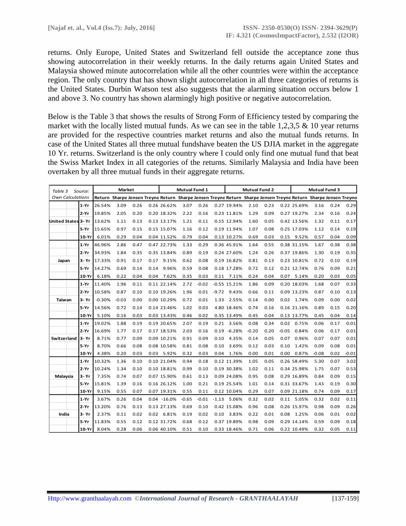
Below is the Table 3 that shows the results of Strong Form of Efficiency tested by comparing the

market with the locally listed mutual funds. As we can see in the table 1,2,3,5 & 10 year returns

are provided for the respective countries market returns and also the mutual funds returns. In

case of the United States all three mutual fundshave beaten the US DJIA market in the aggregate

10 Yr. returns. Switzerland is the only country where I could only find one mutual fund that beat

the Swiss Market Index in all categories of the returns. Similarly Malaysia and India have been

overtaken by all three mutual funds in their aggregate returns.

Return Sharpe Jensen TreynorReturn Sharpe Jensen TreynorReturn Sharpe Jensen TreynorReturn Sharpe Jensen Treynor

1-Yr 26.54% 3.09 0.26 0.26 26.62% 3.07 0.26 0.27 19.94% 2.10 0.23 0.22 25.69% 3.16 0.24 0.29

2-Yr 19.85% 2.05 0.20 0.20 18.32% 2.22 0.16 0.23 11.81% 1.29 0.09 0.27 19.27% 2.34 0.16 0.24

3- Yr 13.62% 1.11 0.13 0.13 13.17% 1.21 0.11 0.15 12.94% 1.60 0.05 0.42 13.56% 1.32 0.11 0.17

5-Yr 15.65% 0.97 0.15 0.15 15.07% 1.16 0.12 0.19 11.94% 1.07 0.08 0.25 17.03% 1.12 0.14 0.19

10-Yr 6.01% 0.29 0.04 0.04 11.52% 0.79 0.04 0.13 10.27% 0.69 0.03 0.15 9.52% 0.57 0.04 0.09

1-Yr 46.96% 2.86 0.47 0.47 22.73% 1.33 0.29 0.36 45.91% 1.64 0.55 0.38 31.15% 1.67 0.38 0.38

2-Yr 34.93% 1.84 0.35 0.35 13.84% 0.89 0.19 0.24 27.60% 1.24 0.26 0.37 19.86% 1.30 0.19 0.35

3- Yr 17.33% 0.91 0.17 0.17 9.15% 0.62 0.08 0.19 16.82% 0.81 0.13 0.23 10.81% 0.72 0.10 0.19

5-Yr 14.27% 0.69 0.14 0.14 9.96% 0.59 0.08 0.18 17.28% 0.72 0.12 0.21 12.74% 0.76 0.09 0.21

10-Yr 6.18% 0.22 0.04 0.04 7.62% 0.35 0.03 0.11 7.11% 0.24 0.04 0.07 5.14% 0.20 0.03 0.05

1-Yr 11.40% 1.96 0.11 0.11 22.14% 2.72 -0.02 -0.55 15.21% 1.86 0.09 0.20 18.03% 1.68 0.07 0.33

2-Yr 10.58% 0.87 0.10 0.10 19.26% 1.96 0.01 -9.72 9.43% 0.66 0.11 0.09 13.23% 0.87 0.10 0.13

3- Yr -0.30% -0.03 0.00 0.00 10.29% 0.72 0.01 1.33 2.55% 0.14 0.00 0.02 1.74% 0.09 0.00 0.02

5-Yr 14.56% 0.72 0.14 0.14 23.46% 1.02 0.03 4.80 18.46% 0.74 0.16 0.16 21.16% 0.89 0.15 0.20

10-Yr 5.10% 0.16 0.03 0.03 13.43% 0.46 0.02 0.35 13.49% 0.45 0.04 0.13 13.77% 0.45 0.04 0.14

1-Yr 19.02% 1.88 0.19 0.19 20.65% 2.07 0.19 0.21 3.56% 0.08 0.34 0.02 0.75% 0.06 0.17 0.01

2-Yr 16.69% 1.77 0.17 0.17 18.53% 2.03 0.16 0.19 -6.28% -0.20 0.20 -0.05 0.84% 0.06 0.17 0.01

3- Yr 8.71% 0.77 0.09 0.09 10.21% 0.91 0.09 0.10 4.35% 0.14 0.05 0.07 0.96% 0.07 0.07 0.01

5-Yr 8.70% 0.66 0.08 0.08 10.58% 0.81 0.08 0.10 3.69% 0.12 0.03 0.10 1.42% 0.09 0.08 0.01

10-Yr 4.38% 0.20 0.03 0.03 5.92% 0.32 0.03 0.04 1.76% 0.00 0.01 0.00 0.87% -0.08 0.02 -0.01

1-Yr 10.32% 1.36 0.10 0.10 21.04% 0.94 0.18 0.12 11.39% 1.05 0.05 0.26 58.49% 5.30 0.07 3.02

2-Yr 10.24% 1.34 0.10 0.10 18.81% 0.99 0.10 0.19 30.38% 1.02 0.11 0.34 25.98% 1.75 0.07 0.53

3- Yr 7.35% 0.74 0.07 0.07 15.90% 0.61 0.13 0.09 24.08% 0.95 0.08 0.29 16.89% 0.84 0.09 0.15

5-Yr 15.81% 1.39 0.16 0.16 26.12% 1.00 0.21 0.19 25.54% 1.01 0.14 0.31 33.67% 1.43 0.19 0.30

10-Yr 9.15% 0.55 0.07 0.07 19.31% 0.55 0.11 0.12 10.04% 0.29 0.07 0.09 21.18% 0.74 0.09 0.17

1-Yr 3.67% 0.26 0.04 0.04 -16.0% -0.65 -0.01 -1.13 5.06% 0.32 0.02 0.11 5.05% 0.32 0.02 0.11

2-Yr 13.20% 0.76 0.13 0.13 27.13% 0.69 0.10 0.42 15.08% 0.96 0.08 0.26 15.97% 0.98 0.09 0.26

3- Yr 2.37% 0.11 0.02 0.02 6.81% 0.19 0.02 0.10 3.83% 0.22 0.01 0.08 1.25% 0.06 0.01 0.02

5-Yr 11.83% 0.55 0.12 0.12 31.72% 0.68 0.12 0.37 19.89% 0.98 0.09 0.29 14.14% 0.59 0.09 0.18

10-Yr 8.04% 0.28 0.06 0.06 40.10% 0.51 0.10 0.33 18.46% 0.71 0.06 0.22 10.49% 0.32 0.05 0.11

Japan

Market

United States

Mutual Fund 3Table 3 Source:

Own Calculations

Taiwan

Switzerland

Malaysia

India

Mutual Fund 1 Mutual Fund 2





Furthermore Sharpe, Jenson and Treynor ratios were calculated for all indices and mutual funds.

The risk free rate posed a great challenge as the data for risk free rate (in our case 3-month

treasury bill) for each country was not available. While researching in one of the articles written

by Prof A.Q Khan and Sana Ikram in 2011 suggests that in reality no rate is risk free rate. The

best proxy that can be used for risk free rate is the US 3-month Treasury bill. The above

mentioned experiments were conducted on the following 10 United States Macroeconomic

Variables.

Table 5: Infl Gold IPI ST int Oil LT

Int

Unemploy DOW EUR M2

No. of values used 119 119 119 119 119 119 119 119 119 119

Range 0.031 0.235 0.058 4.175 0.617 0.506 0.12286 0.236 0.1408 0.483

Mean 0.002 0.01 9E-04 0.056 0.013 -0 0.0017 0.005 -

0.0004

0.025

Kurtosis 8.8 0.229 8.128 18.78 1.899 3.153 0.50197 1.723 0.7267 -1.59

Skewness -1.46 -0 -2.14 3.681 -0.61 -0.53 0.83272 -0.76 0.4174 0.114

variance 1E-05 0.002 6E-05 0.248 0.009 0.005 0.0007 0.002 0.0006 0.036

Std deviation 0.004 0.043 0.008 0.498 0.095 0.072 0.02644 0.039 0.024 0.19

KolmogorovSmirnov 0.134 0.04 0.144 0.311 0.075 0.075 0.20625 0.071 0.0667 0.234

P-Value 0.028 0.992 0.014 <0.0001 0.518 0.511 < 0.0001 0.584 0.664 <0.0001

Table 5 shows the descriptive statistics of the 10 variables and Dow Jones Industrial Average

(DJIA) can deviate by 3.9%. When the P-value of any given variable is less than the confidence

interval we reject the null hypothesis that the sample resembles a normal population. From

looking at the data above we can see that the P-Value for ST Int, Unemployment and Money

Supply (M2) are below significance level of 0.01 while inflation and Industrial Production are

below the significance level of 0.05. Thus in total 5 variables Short Term Interest Rate,

Unemployment, Money Supply, Inflation and Industrial Production fail the Kolmogorov-

Smirnov Test.

Return Sharpe Jensen TreynorReturn Sharpe Jensen TreynorReturn Sharpe Jensen TreynorReturn Sharpe Jensen Treynor

1-Yr 3.67% 0.26 0.04 0.04 9.07% 0.54 0.04 0.08 13.06% 1.04 0.02 0.32 44.20% 1.10 0.02 -0.93

2-Yr 13.20% 0.76 0.13 0.13 21.68% 1.11 0.12 0.25 20.15% 1.63 0.06 0.57 22.62% 0.70 -0.01 -0.91

3- Yr 2.37% 0.11 0.02 0.02 5.68% 0.23 0.03 0.05 8.51% 0.65 0.01 0.24 5.62% 0.19 0.01 0.52

5-Yr 11.83% 0.55 0.12 0.12 29.84% 0.95 0.15 0.24 20.98% 1.09 0.07 0.40 17.40% 0.42 0.03 0.93

10-Yr 8.04% 0.28 0.06 0.06 12.25% 0.36 0.07 0.10 4.96% 0.16 0.04 0.06 3.98% 0.06 0.02 0.08

1-Yr 17.42% 1.31 0.17 0.17 2.67% 1.84 0.01 0.35 7.83% 1.65 0.05 0.31 8.43% 1.78 0.05 0.33

2-Yr 15.79% 1.09 0.16 0.16 3.75% 2.43 0.01 0.47 11.42% 2.05 0.05 0.45 12.03% 2.16 0.05 0.48

3- Yr 5.05% 0.28 0.05 0.05 2.70% 1.40 0.00 0.80 4.81% 0.65 0.02 0.15 5.41% 0.74 0.02 0.17

5-Yr 6.66% 0.33 0.06 0.06 2.53% 1.38 0.00 1.11 9.08% 1.23 0.02 0.33 9.68% 1.31 0.02 0.35

10-Yr 2.42% 0.04 0.01 0.01 2.70% 0.57 0.00 -2.40 4.21% 0.30 0.00 0.07 4.81% 0.37 0.01 0.08

1-Yr 9.45% 1.18 0.09 0.09 42.41% 1.63 0.13 0.37 13.31% 1.84 0.08 0.17 26.86% 3.08 0.08 0.39

2-Yr 6.90% 0.78 0.07 0.07 3.99% 0.13 0.09 0.03 9.75% 0.87 0.08 0.09 22.22% 2.09 0.07 0.24

3- Yr 0.96% 0.08 0.01 0.01 -1.79% -0.08 0.01 -0.02 2.16% 0.15 0.01 0.02 9.39% 0.67 0.02 0.09

5-Yr 9.14% 0.70 0.09 0.09 19.66% 0.58 0.15 0.12 14.40% 0.96 0.06 0.26 18.07% 1.06 0.10 0.18

10-Yr 5.69% 0.28 0.04 0.04 7.98% 0.18 0.06 0.04 3.78% 0.12 0.02 0.05 5.74% 0.21 0.04 0.04

1-Yr 6.79% 0.48 0.07 0.07 11.25% 0.35 0.12 0.06 12.15% 0.73 0.07 0.11 12.15% 0.73 0.07 0.11

2-Yr 16.18% 1.01 0.16 0.16 38.48% 1.06 0.33 0.19 20.91% 1.07 0.18 0.18 20.91% 1.07 0.18 0.18

3- Yr -2.65% -0.15 -0.03 -0.03 -1.54% -0.04 -0.05 -0.01 1.28% 0.05 -0.03 0.01 1.28% 0.05 -0.03 0.01

5-Yr 9.89% 0.44 0.10 0.10 24.48% 0.45 0.20 0.12 15.71% 0.50 0.13 0.12 15.71% 0.50 0.13 0.12

10-Yr 6.85% 0.21 0.05 0.05 10.67% 0.20 0.08 0.06 9.60% 0.26 0.06 0.07 9.60% 0.26 0.06 0.07

1-Yr 14.53% 1.17 0.14 0.14 32.84% 1.51 0.21 0.23 29.71% 1.32 0.23 0.19 37.94% 1.74 0.19 0.32

2-Yr 13.90% 1.21 0.14 0.14 30.12% 1.61 0.19 0.23 32.29% 1.72 0.19 0.24 26.04% 1.39 0.15 0.25

3- Yr 4.03% 0.32 0.04 0.04 18.32% 0.99 0.06 0.15 20.83% 1.10 0.06 0.17 12.89% 0.67 0.05 0.12

5-Yr 8.52% 0.61 0.08 0.08 23.01% 1.04 0.12 0.17 21.46% 0.97 0.11 0.17 12.45% 0.40 0.11 0.09

10-Yr 5.87% 0.29 0.04 0.04 13.52% 0.58 0.04 0.13 14.24% 0.63 0.05 0.12 13.45% 0.37 0.04 0.14

1-Yr 16.70% 1.34 0.17 0.17 22.67% 1.98 0.16 0.25 21.27% 1.63 0.16 0.22 21.06% 1.55 0.17 0.21

2-Yr 13.35% 1.08 0.13 0.13 19.97% 1.81 0.12 0.22 20.03% 1.50 0.13 0.21 19.24% 1.38 0.14 0.19

3- Yr 5.19% 0.35 0.05 0.05 10.35% 0.77 0.05 0.11 7.68% 0.45 0.05 0.07 7.71% 0.44 0.05 0.07

5-Yr 11.29% 0.64 0.11 0.11 15.59% 0.94 0.11 0.16 8.77% 0.45 0.11 0.09 8.14% 0.40 0.10 0.08

10-Yr 2.98% 0.06 0.01 0.01 8.72% 0.40 0.02 0.07 3.67% 0.11 0.01 0.02 3.21% 0.08 0.01 0.02

Amsterdam

Hong Kong

Europe

Canada

Austria

Australia

Table 4 Source:

Own Calculations

Market Mutual Fund 1 Mutual Fund 2 Mutual Fund 3





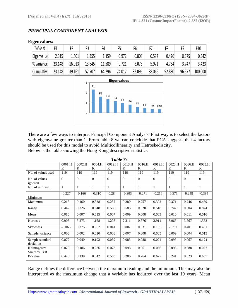
PRINCIPAL COMPONENT ANALYSIS

Eigenvalues:

There are a few ways to interpret Principal Component Analysis. First way is to select the factors

with eigenvalue greater than 1. From table 8 we can conclude that PCA suggests that 4 factors

should be used for this model to avoid Multicollinearity and Hetroskediscity.

Below is the table showing the Hong Kong descriptive statistics

Table 7: 0001.H

K

0002.H

K

0004.H

K

0012.H

K

0013.H

K

0016.H

K

0019.H

K

0023.H

K

0066.H

K

0083.H

K

No. of values used 119 119 119 119 119 119 119 119 119 119

No. of values

ignored

0 0 0 0 0 0 0 0 0 0

No. of min. val. 1 1 1 1 1 1 1 1 1 1

Minimum

-0.227 -0.166 -0.310 -0.284 -0.303 -0.271 -0.216 -0.371 -0.258 -0.385

Maximum 0.215 0.160 0.338 0.282 0.280 0.257 0.302 0.371 0.246 0.439

Range 0.442 0.326 0.648 0.566 0.583 0.528 0.518 0.742 0.504 0.824

Mean 0.010 0.007 0.015 0.007 0.009 0.008 0.009 0.010 0.011 0.016

Kurtosis 0.903 5.273 1.168 1.208 2.211 0.876 2.911 3.965 3.567 1.563

Skewness -0.063 0.375 0.062 0.041 0.007 0.031 0.195 -0.211 0.401 0.401

Sample variance 0.006 0.002 0.010 0.008 0.007 0.008 0.005 0.009 0.004 0.015

Sample standard

deviation

0.079 0.040 0.102 0.089 0.085 0.088 0.071 0.093 0.067 0.124

Kolmogorov-

Smirnov Test

0.078 0.106 0.086 0.073 0.098 0.061 0.066 0.095 0.088 0.067

P-Value 0.475 0.139 0.342 0.563 0.206 0.764 0.677 0.241 0.323 0.667

Range defines the difference between the maximum reading and the minimum. This may also be

interpreted as the maximum change that a variable has incurred over the last 10 years. Mean

Table 8 F1 F2 F3 F4 F5 F6 F7 F8 F9 F10

Eigenvalue 2.315 1.601 1.355 1.159 0.972 0.808 0.597 0.476 0.375 0.342

% variance 23.148 16.013 13.545 11.589 9.721 8.078 5.971 4.764 3.747 3.423

Cumulative % 23.148 39.161 52.707 64.296 74.017 82.095 88.066 92.830 96.577 100.000

F1

F2 F3

F4 F5

F6 F7 F8 F9 F10

0

1

2

3Eigenvalues





signifies the average of a company’s return over the last 10 years. In terms of kurtosis none of

the variables in the first table are close to zero. All positive readings for kurtosis indicate a

Leptokurtic shape of the sample distribution.

Variable R² F Test Intercept LT Int ^HIS Exchange GOLD

0001.HK: 0.757 < 0.0001 0.002 -0.002 1.093 0.987 -0.007

0.548 0.944 < 0.0001 0.754 0.934

0002.HK 0.086 0.037 0.005 -0.017 0.105 7.201 0.169

0.189 0.443 0.078 0.020 0.046

0003.HK 0.646 < 0.0001 0.003 -0.011 1.298 -0.549 0.203

0.563 0.760 < 0.0001 0.911 0.133

0004.HK 0.646 < 0.0001 0.003 -0.011 1.298 -0.549 0.203

0.563 0.760 < 0.0001 0.911 0.133

0012.HK 0.682 < 0.0001 -0.002 -0.006 1.194 7.799 0.121

0.638 0.843 < 0.0001 0.057 0.278

0013.HK 0.626 < 0.0001 0.001 0.062 1.037 1.182 -0.017

0.793 0.044 < 0.0001 0.779 0.885

0016.HK 0.665 < 0.0001 -0.002 -0.003 1.148 4.608 0.206

0.642 0.907 < 0.0001 0.264 0.070

0019.HK 0.559 < 0.0001 0.002 0.026 0.846 6.164 0.098

0.682 0.347 < 0.0001 0.107 0.350

0023.HK 0.620 < 0.0001 0.000 0.035 1.177 13.892 0.208

0.943 0.292 < 0.0001 0.003 0.104

0066.HK 0.537 < 0.0001 0.003 -0.010 0.787 6.536 0.252

0.495 0.719 < 0.0001 0.078 0.014

0083.HK 0.598 < 0.0001 0.003 -0.075 1.570 9.544 0.244

0.689 0.106 < 0.0001 0.137 0.165

0101.HK 0.483 < 0.0001 0.007 -0.063 -0.063 1.036 1.284

0.322 0.109 < 0.0001 0.813 0.505

0291.HK 0.505 < 0.0001 0.007 -0.048 1.125 13.297 -0.009

0.325 0.226 < 0.0001 0.016 0.955

0293.HK 0.550 < 0.0001 0.000 0.034 0.951 7.459 -0.071

0.966 0.279 < 0.0001 -0.019 0.552

0388.HK 0.646 < 0.0001 0.011 0.070 1.421 -15.479 0.303

0.110 0.102 < 0.0001 0.010 0.063

0494.HK 0.238 < 0.0001 0.004 0.007 0.667 -8.450 0.139

0.641 0.883 < 0.0001 0.208 0.449

0762.HK 0.259 < 0.0001 0.001 -0.063 0.696 -5.336 0.216

0.901 0.175 < 0.0001 0.406 0.219

0836.HK 0.389 < 0.0001 0.022 -0.103 0.903 12.282 -0.681





Table above is the regression for Hong Kong Stock Exchange. . The Independent variables are

International Gold Prices in Honk Kong Dollars, Long Term Interest Rate, Exchange Rate with

the US and Hang Seng 50 Index Return. The dependent variable is the monthly returns of Hang

Seng 50 Index. The R2 for Hong Kong Stock Exchange seems much more promising than The

United States.%. The P-Value of F Test which is provided in the 2nd

column suggests that except

for 0006.HK and 0883.HK the model is insignificant. For these companies the percentage of

variance explained in the stock price is 0.9% and 6.7%. For LT Int the significant negative

impact was in the case of 0101.HK (-0.063) and significant positive impact in case of 0388.HK

(0.070). Just like the United Stated the most important macroeconomic variable that represents

the most variance in stock prices is Hang Seng 50 Index Return. The only company that had a

significant negative impact was 0101.HK of -0.063. Rest all of the companies are positively

correlated except for 0883.HK which had no significant impact from the Hang Seng 50 Index

return. The beta for exchange rate ranged from -15.479 for 0388.HK to 22.378 for 0027.HK. The

beta for Gold prices ranged from -0.681 for 0836.HK to 1.284 for 0101.HK.

5. CONCLUSION & RECOMMENDATIONS

10 variables were initially selected for the purpose of building the Arbitrage Pricing Model.

These were Inflation, Gold Prices, Industrial Production Index, Short Term Interest Rates, Oil

Prices, Long Term Interest Rates, Unemployment, Dow Jones Industrial Average, Exchange

Rate (EUR) and Money Supply. Correlation matrix was applied to the 10 variables to avoid

Multicollinearity. Furthermore, Principal Component Analysis was applied to reduce the number

of variables to those that represented the most variance in the other variables. PCA suggested

that 4 variables should be utilized from the 10 initially selected variables. The factor loadings

from PCA showed that Gold Prices, Long Term Interest Rate, Dow Jones Industrial Index and

Exchange Rate should represent the APT Model.

The Ordinary Least Square Regression (Saeed & Akhter, 2010) was applied to study the linear

relationship between the independent and dependent variables. Similar model was applied on

both Hong Kong and United States Stock Exchange Indices. For the United States 3/29

companies showed a value of R2 more than 60%. And 3 out of the remaining 26 companies

produce a variance above 50%. These results are not sufficient enough to generalize the APT

model for the United States Stock Exchange. The Hong Kong Stock Exchange produced better

results than the US. Hong Kong had one out of 40 companies with R2 value above 70%, 11

companies were above 60% and 9 companies above 50%. These results though better than the

US still not sufficient enough for the APT to become a valid predictor of stock returns.

From the above discussion we can conclude that APT was successful in explaining some of the

variance in these markets. The most important point to note here is that as the efficiency of stock

exchanges increase, APT’s performance starts to get better. In case of United States the variance

explained was not as high as variance explained by the Hong Kong Model. Thus we can

conclude that Arbitrage Pricing Model is linked with market efficiency. This thesis also

concludes that the existence of a perfectly efficient market is not possible. Even though Hong

Kong Stock Exchange was picked as the proxy for efficient market, its efficiency is still

questionable.





My recommendation is that users of Arbitrage or any other pricing model, should first relate the

asset pricing theory with market efficiency, in order to predict their effectiveness in a given

market. Inefficient market failed to produce viable results. This is a sign that asset pricing theory

such as APT may not be a successful predictor of stock returns.

6. REFERENCES

[1] Ikram, S., & Khan, A. Q. (2011). Testing Strong Form Market Efficiency of Indian

Capital Market: Performance Appraisal of Mutual Funds. International Journal of

Business and Information Technology, 1(2).

[2] Hyde, S.J. (2007). The resposne of Industry stock returns to market, exchange rate and

interest rate risks, Managerial Finance, pp. 693-709.

[3] Ihsan, H., Ahmad, E., Haq, M.I.U., and Sadia, H. (2007). Relationship of Economic and

Financial Variables with Behaviors of Stock Returns, Journal of Economic Corporation,

28(2), 1-24.

[4] Iqbal, J., & Haider, A. (2005). Arbitrage pricing theory: evidence from an emerging

stock market. Munich Personal RePEc Archive, 10(1), 123-139.

[5] Iqbal, Naeem, Khattak, Sajid Rehman, Khattak, M. Arif and Ullah, Innayat (2012).

Testing the Arbitrage Pricing Theory on Karachi Stock Exchange, Interdisciplinary

Journal of Contemporary Research in Business, 4(8).

[6] Iqbal, Javed, and Haider, Aziz (2005). Arbitrage Pricing Theory: Evidence From An

Emerging Stock Market, Munich Personal RePEc Archive, 10(1), 123-139.

[7] Jaffe F. Jaffery, (Jul.1974), Special Information and Insider Trading, The Journal of

Business, 47(3), pp. 410-428.

[8] Jaffe, J., & Randolph Westerfield, R. (2004). Corporate finance. Tata McGraw-Hill

Education.

[9] Jagannathan, Ravi, Keiichi Kubota, and Hitoshi Takehara, (1998). Relationship between

Labor-Income Risk and Average Return: Empirical Evidence from the Japanese Stock

Market, Journal of Business, 3(71), 319-347.

[10] Jegadeesh, N., & Titman, S. (1993). Returns to buying winners and selling losers:

Implications for stock market efficiency. The Journal of Finance, 48(1), 65-91.

[11] Javid, Attiya Yasmin, (2008a). Time Varying Risk Return Relationship: Evidence from

listed Pakistani Firms, European Journal of Scientific Research, 22(1), 16-39.

[12] Jolliffe, I. T. (1972). Discarding variables in a principal component analysis. I: Artificial

data. Applied statistics, 160-173.

[13] Jones, T. L., Fu, X., & Tang, T. (2008). Day-of-the-week effect in the seasoned equity

offering discount. Managerial Finance, 35(1), 48-62.

[14] Joulion, P. (1991). Pacing of Exchange Rate Risk in the Stock Market, Journal of

Financial and Quantitative Analysis, 26, 363–76.

[15] Karras, G., Lee, J. M., & Neuburger, H. (2007). Unlocking the sources of the apparent

episodic stationarity of the P/E ratio: Impulses or propagation? Review of Accounting

and Finance, 6(3), 339-348.

[16] Kaur, D., & Sahu, N. G. (2009). Correlation and causality between stock market and

macroeconomic variables in India: an empirical study.





[17] Khan, M. A., Qayyum, A., Sheikh, S. A., & Siddique, O. (2005). Financial Development

and Economic Growth: The Case of Pakistan [with Comments].The Pakistan

Development Review, 819-837.

[18] Khilji, N. M. (1993). The behavior of stock return in an emerging market: A case study of

Pakistan. Pakistan Development Review, 32 (4), 593-604.

[19] Kim, H. J. (2008). Common factor analysis versus principal component analysis: choice

for symptom cluster research. Asian Nursing Research, 2(1), 17-24.

[20] King, J. R., & Jackson, D. A. (1999). Variable selection in large environmental data sets

using principal components analysis. Environmetrics, 10(1), 67-77.

[21] Lee, B. S. (1992), Causal Relations among Stock Returns, Interest Rates, Real Activity,

and Inflation, The J. Finance, 47(4): 1591-1603.

[22] Lee, W. (1997). Market timing and short-term interest rates. Journal of Portfolio

Management, 23 (3), 35-46.

[23] Adam, A. M., Tweneboah, G., (2007). Macroeconomic Factors and Stock Market

Movement: Evidence from Ghana, School of Management, University of Leicester, UK.

[24] Adler and B. Domas. (1983). International Portfolio choice and Corporation: A

Synthesis. Journal of Finance, 38, 925–984.

[25] Affleck-Graves, J. F. and Money, A. H. (1975). A Note on the Random Walk Model and

South African Share Prices. The South African Journal of Economics, 43(3), 382-388.

[26] Aggarwal, R. (1981). Exchange rates and stock prices: A study of the US capital markets

under floating exchange rates, Akron Business and Economic Review, 12, pp. 7-12.

[27] Ahmad Eatzaz and Badar-u-Zaman (1999). Volatility and Stock Return at Karachi Stock

Exchange, Pakistan Economic and Social Review, 37(1), 25–37.

[28] Ahmed, M.A., Rehman, R.U., Raoof, A. (2010). Do interest rates, Exchange Rates effect

Stock Returns? A Pakistani Perspective, International Research Journal of Finance and

Economics, (50), pp. 146-150.

[29] Alam, M. M., & Uddin, M. G. S. (2009). Relationship between interest rate and stock

price: empirical evidence from developed and developing countries, International journal

of business and management, 4(3), P43.

[30] Ali, Imran, et al. "Causal relationship between macro-economic indicators and stock

exchange prices in Pakistan." African Journal of Business Management4.3 (2010): 312-

319.


arbitrage pricing model in relation to...

Documents