ar and ma models - amazon s3...ar and ma together: arma > x plot(x, main = "arma(1,...
TRANSCRIPT

ARIMA MODELING WITH R
AR and MA Models

ARIMA Modeling with R
AR and MA Models> x <- arima.sim(list(order = c(1, 0, 0), ar = -.7), n = 200) > y <- arima.sim(list(order = c(0, 0, 1), ma = -.7), n = 200)
> par(mfrow = c(1, 2)) > plot(x, main = "AR(1)") > plot(y, main = "MA(1)")
AR(1)
Time
x
0 50 100 150 200
−3−2
−10
12
34
MA(1)
Time
y
0 50 100 150 200
−3−2
−10
12
3
ARIMA Modeling with R
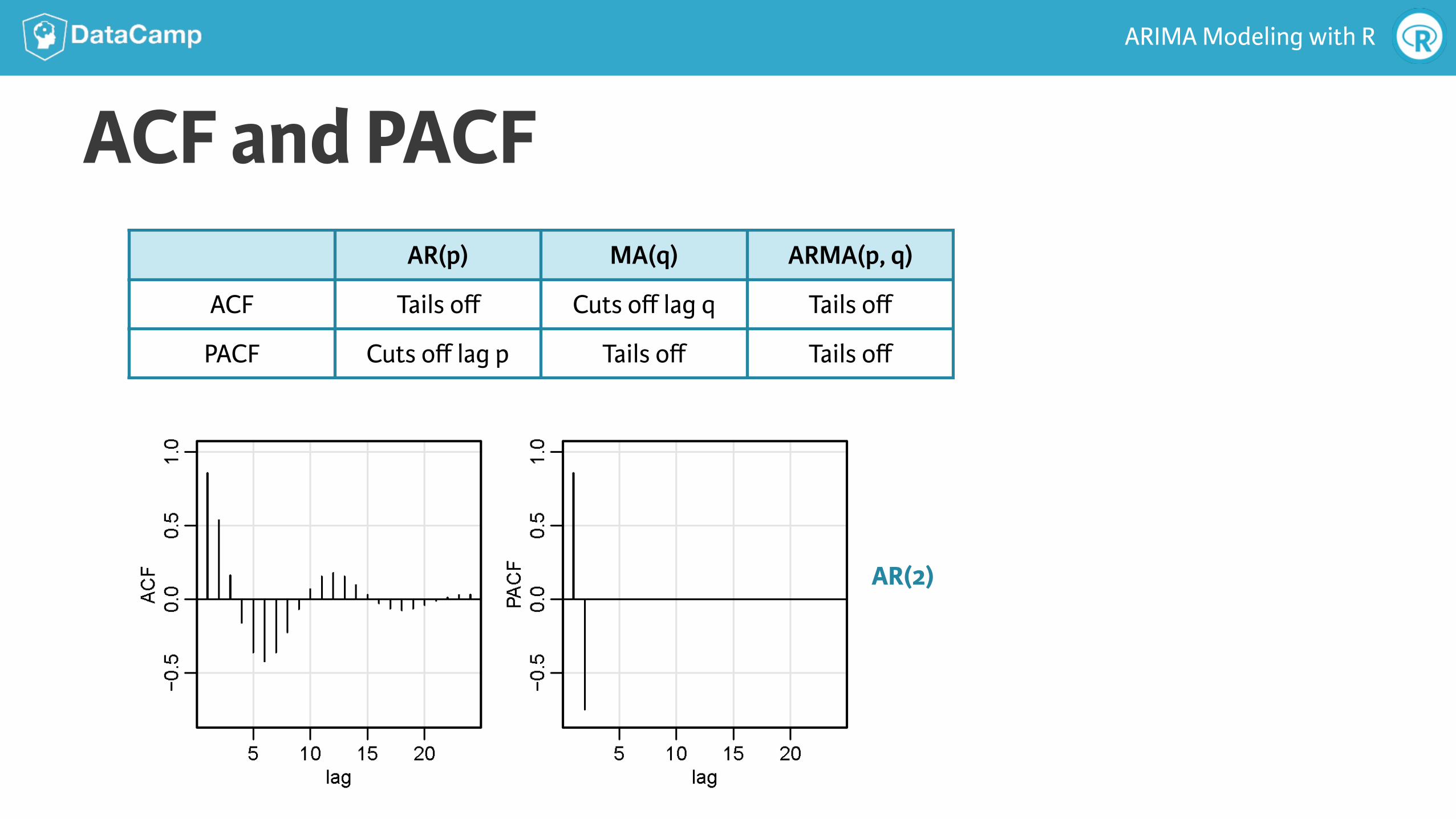
ACF and PACFAR(p) MA(q) ARMA(p, q)
ACF Tails off Cuts off lag q Tails off
PACF Cuts off lag p Tails off Tails off
AR(2)

ARIMA Modeling with R
MA(1)
ACF and PACFAR(p) MA(q) ARMA(p, q)
ACF Tails off Cuts off lag q Tails off
PACF Cuts off lag p Tails off Tails off

ARIMA Modeling with R
Estimation● Estimation for time series is similar to using least squares
for regression
● Estimates are obtained numerically using ideas of Gauss and Newton
ARIMA Modeling with R
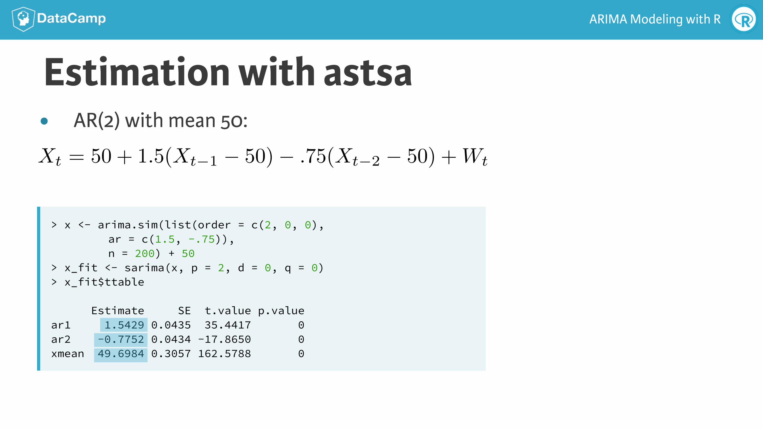
Estimation with astsa
> x <- arima.sim(list(order = c(2, 0, 0), ar = c(1.5, -.75)), n = 200) + 50
> x_fit <- sarima(x, p = 2, d = 0, q = 0) > x_fit$ttable
Estimate SE t.value p.value ar1 1.5429 0.0435 35.4417 0 ar2 -0.7752 0.0434 -17.8650 0 xmean 49.6984 0.3057 162.5788 0
● AR(2) with mean 50:
Xt = 50 + 1.5(Xt�1 � 50)� .75(Xt�2 � 50) +Wt
ARIMA Modeling with R
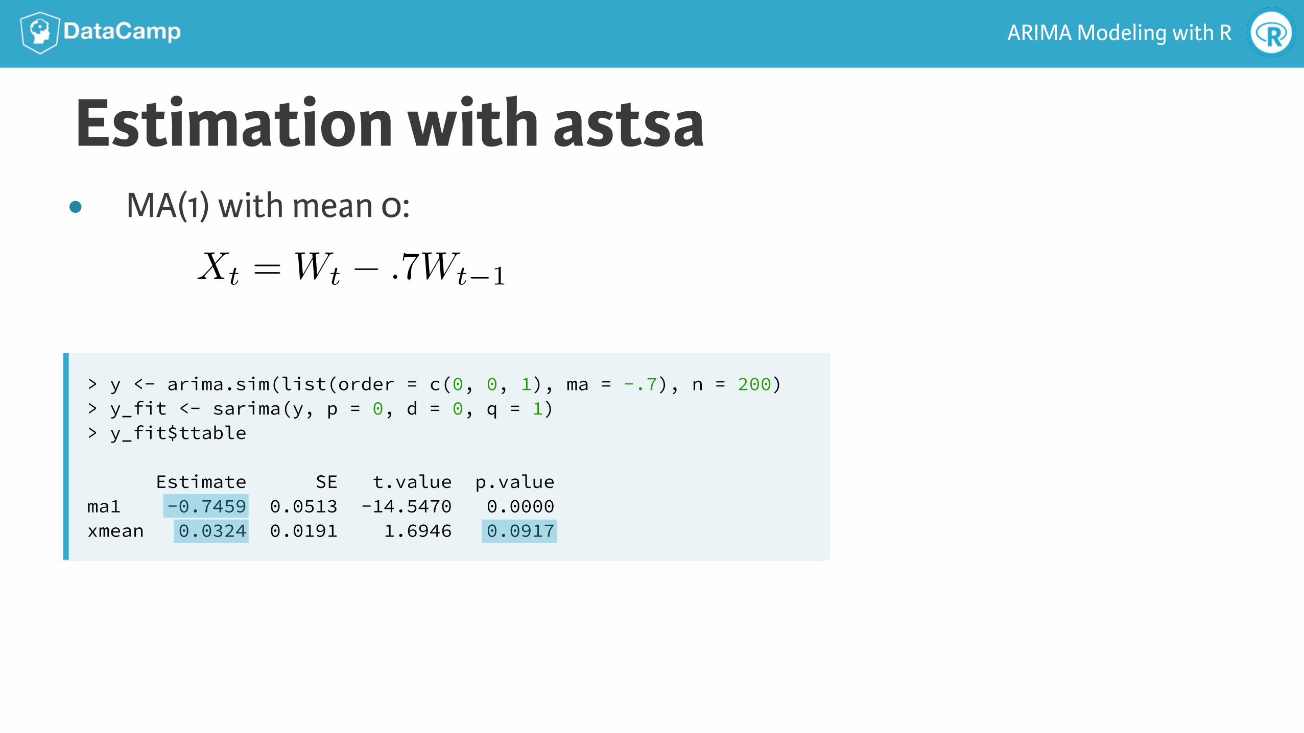
Estimation with astsa
> y <- arima.sim(list(order = c(0, 0, 1), ma = -.7), n = 200) > y_fit <- sarima(y, p = 0, d = 0, q = 1) > y_fit$ttable
Estimate SE t.value p.value ma1 -0.7459 0.0513 -14.5470 0.0000 xmean 0.0324 0.0191 1.6946 0.0917
● MA(1) with mean 0:
Xt = Wt � .7Wt�1

ARIMA MODELING WITH R
Let’s practice!

ARIMA MODELING WITH R
AR and MA Together

ARIMA Modeling with R
AR and MA Together: ARMA
> x <- arima.sim(list(order = c(1, 0, 1), ar = .9, ma = -.4), n = 200) > plot(x, main = "ARMA(1, 1)")
ARMA(1,1)
Time
x
0 50 100 150 200
−4−2
02
4
auto-regression with correlated errors
Xt = �Xt�1 +Wt + ✓Wt�1

ARIMA Modeling with R
ACF and PACF of ARMA ModelsAR(p) MA(q) ARMA(p, q)
ACF Tails off Cuts off lag q Tails off
PACF Cuts off lag p Tails off Tails off
Xt = .9Xt�1 +Wt � .4Wt�1
ARIMA Modeling with R
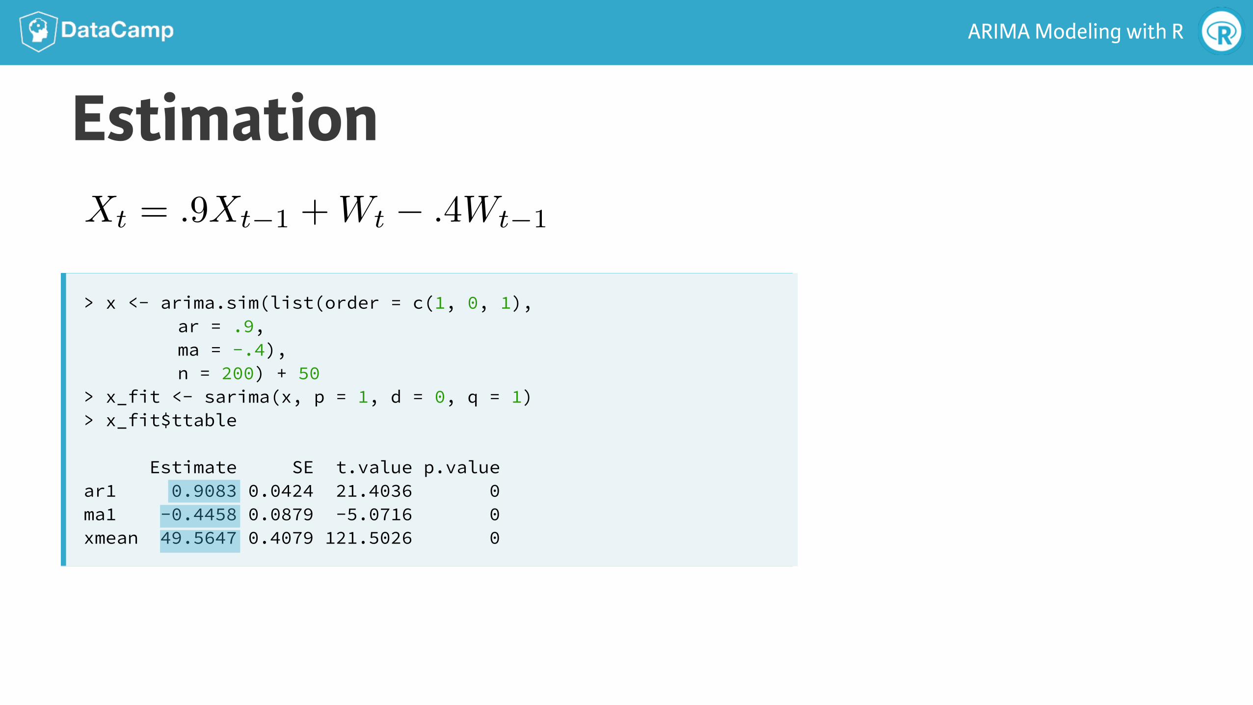
Estimation
> x <- arima.sim(list(order = c(1, 0, 1), ar = .9, ma = -.4), n = 200) + 50
> x_fit <- sarima(x, p = 1, d = 0, q = 1) > x_fit$ttable
Estimate SE t.value p.value ar1 0.9083 0.0424 21.4036 0 ma1 -0.4458 0.0879 -5.0716 0 xmean 49.5647 0.4079 121.5026 0
Xt = .9Xt�1 +Wt � .4Wt�1

ARIMA MODELING WITH R
Let’s practice!

ARIMA MODELING WITH R
Model Choice and Residual Analysis
ARIMA Modeling with R
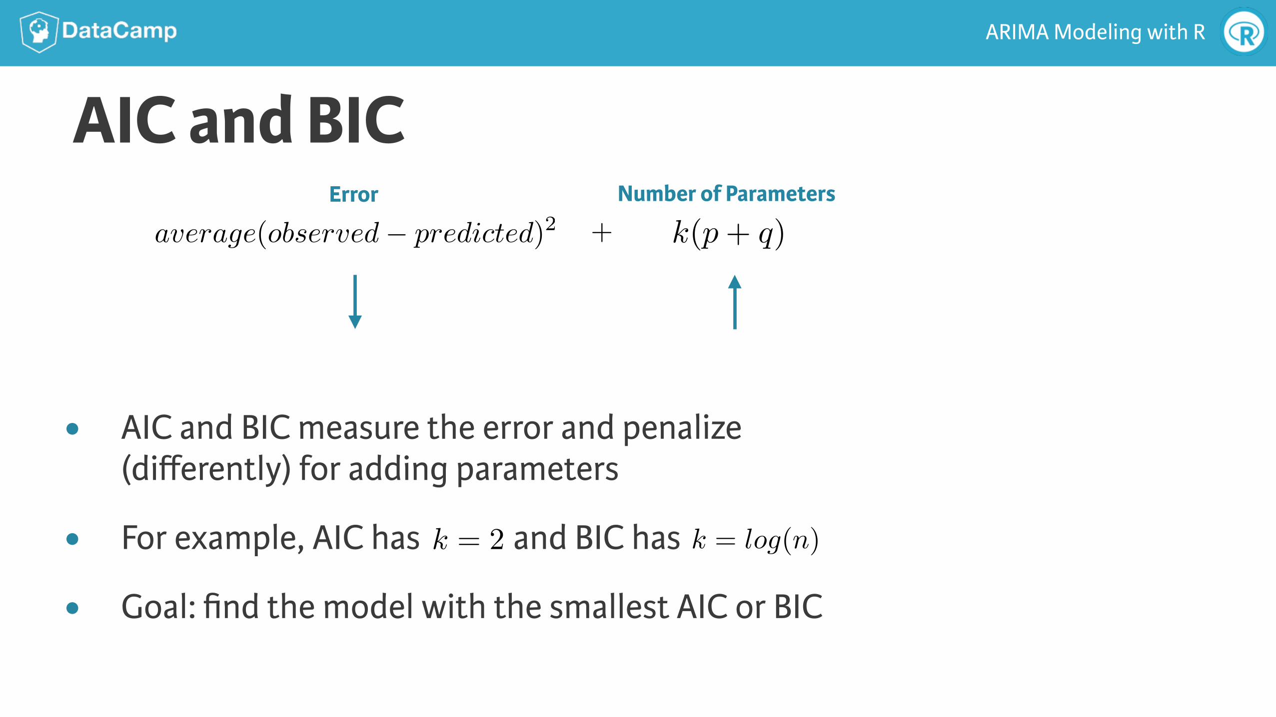
AIC and BIC
● AIC and BIC measure the error and penalize (differently) for adding parameters
● For example, AIC has and BIC has
● Goal: find the model with the smallest AIC or BIC
k = 2 k = log(n)
Error
average(observed� predicted)2Number of Parameters
k(p+ q)+
ARIMA Modeling with R
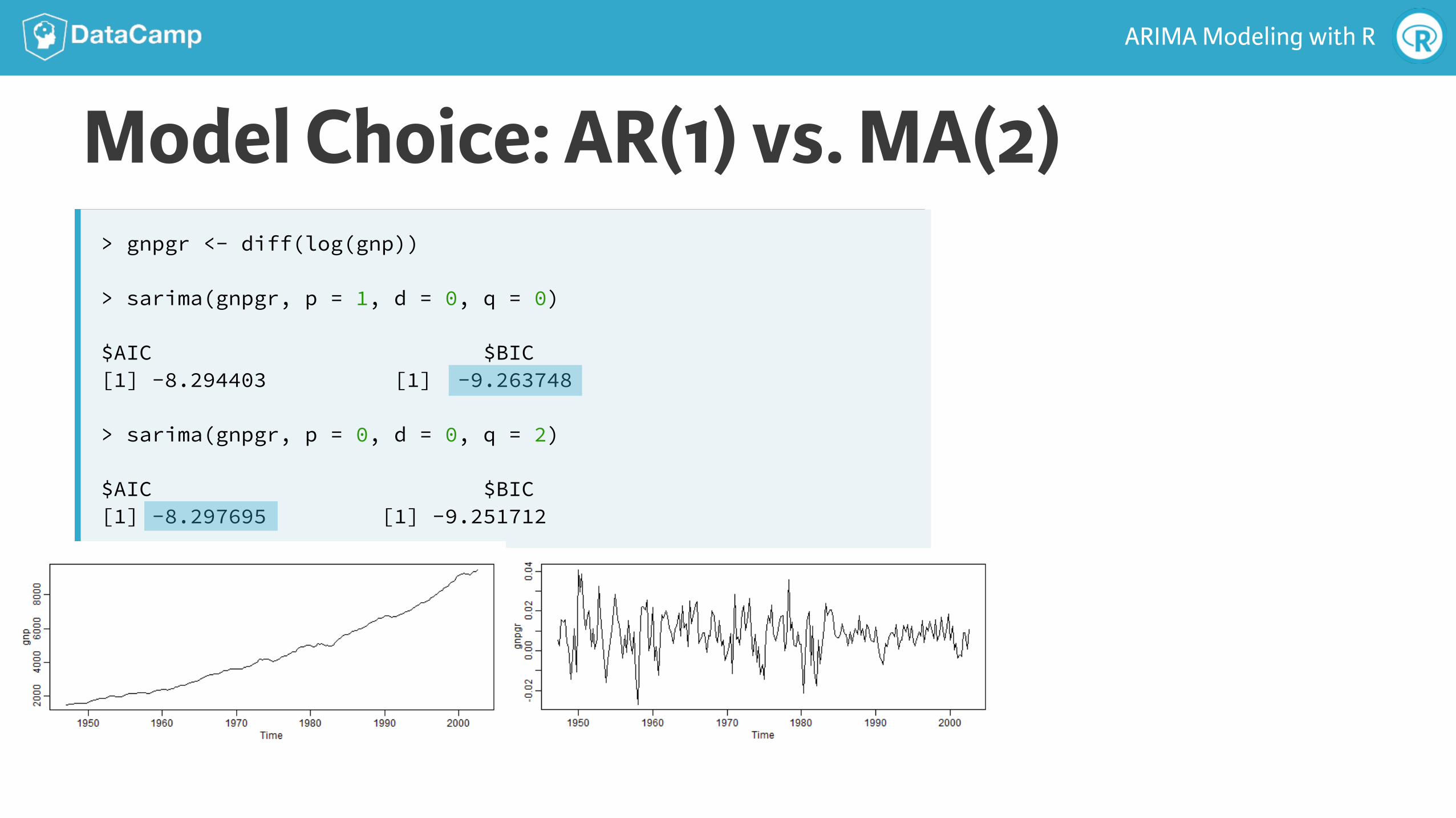
Model Choice: AR(1) vs. MA(2)> gnpgr <- diff(log(gnp))
> sarima(gnpgr, p = 1, d = 0, q = 0)
$AIC $BIC [1] −8.294403 [1] −9.263748
> sarima(gnpgr, p = 0, d = 0, q = 2)
$AIC $BIC [1] −8.297695 [1] −9.251712

ARIMA Modeling with R
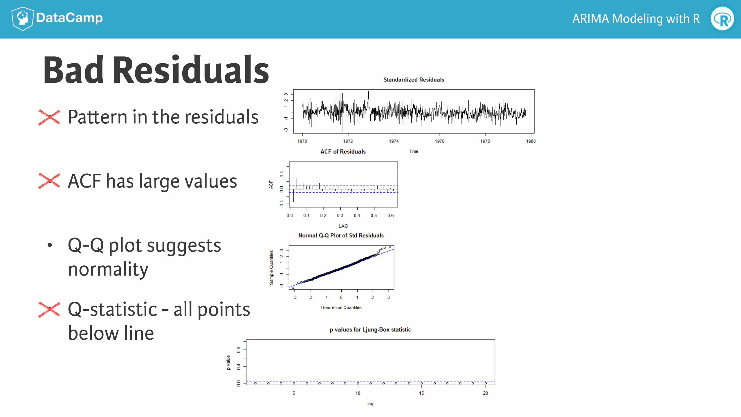
Residual Analysissarima() includes residual analysis graphic showing:
1. Standardized residuals
2. Sample ACF of residuals
3. Normal Q-Q plot
4. Q-statistic p-values
ARIMA Modeling with R
Bad Residuals• Pa"ern in the residuals
• ACF has large values
• Q-Q plot suggests normality
• Q-statistic - all points below line

ARIMA MODELING WITH R
Let’s practice!