www.le.ac.uk

Approximation of heavy models using Radial Basis FunctionsGraeme Alexander (Deloitte)Jeremy Levesley (Leicester)

The problem• Calculate Value at Risk• Need to determine 0.5th percentile of

insurer’s net assets in one year• Net assets = f(R1,R2,R3,...Rn)• Many firms have previously calculated the

percentiles of univariate distns, and aggregated using correlation matrix / copula approach

Moving to Solvency II• For internal model approach, strongly encouraged to

calculate the whole distribution of Net Assets, not just the percentile

• It is a simple matter to generate 100,000 simulations of (R1,R2,..Rn)

• However, evaluating f(r1,r2,..rn) for a single realisation of the risk vector using the “heavy model” can take hours!!

• Common approach: Run the heavy models on a small number of points, and interpolate to obtain estimator function fE(r1, r2, ..,rn), known as a “lite model”

Splines

Linear spline approximation to sin(x)

Combination of hat functions

Cubic Splines

Cubic spline approximation to sin(x)

Combination of B-splines

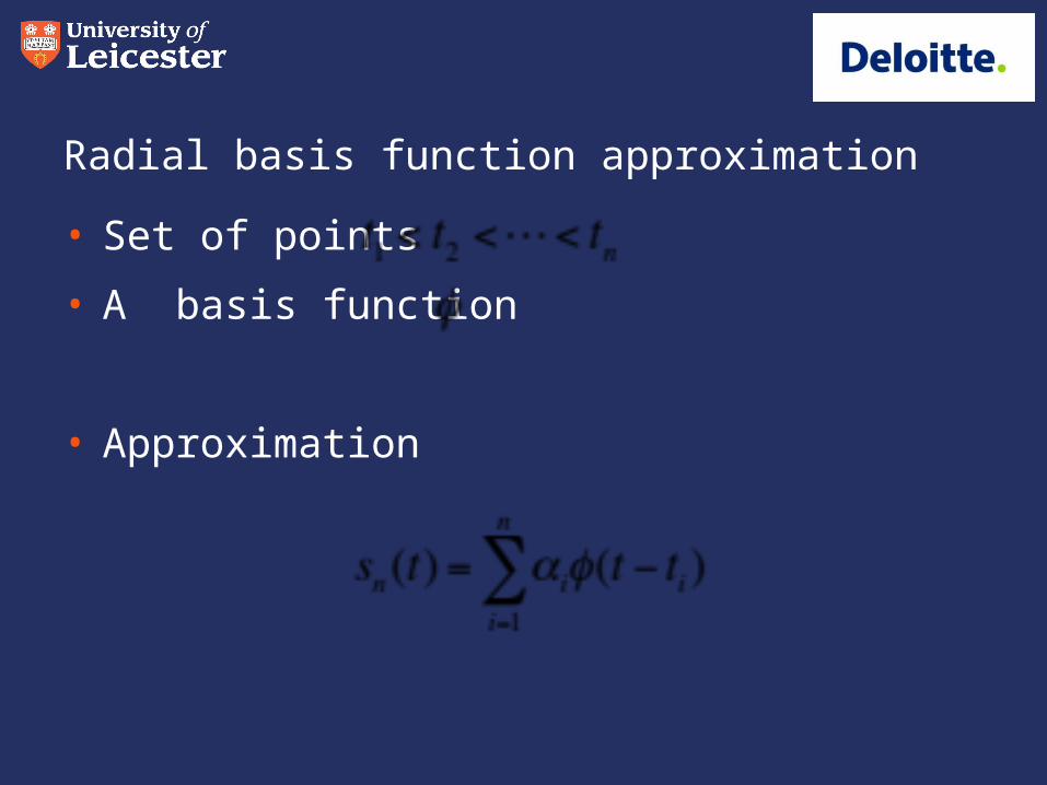
Radial basis function approximation• Set of points• A basis function

• Approximation

More generally

Data Y

x

Gaussian

Yy

yn yxxs )(

)exp()( 22rcr y

yx

How to compute coefficients Interpolation

Linear Equations

.),()( Yxxfxsn

)(

)()(

2

1

2

1

21

22212

12111

nnnnnn

n

n

yf

yfyf

yyyyyy

yyyyyyyyyyyy

An Example - annuity• Difficult to test our interpolation on real-life data due to the length of time

it takes to run heavy models• So let’s take a simple product, a single life annuity, £1 payable p.a.• Assume just two risk factors, discount rate and mortality• Assume a constant rate of mortality 1/T in each future year. Thus, the cash

flows are:(T-1)/T at the end of year 1, (T-2)/T at end of year 2,1 / T at end of year T-1

T

T

t

t

discdiscTdisc

disc

discTtPV

)1(11

.11

)1(1

2

1

1

• Allow T and disc to vary stochasticallydisc~ N (8%, 2.5%2) T ~ N (20,9)

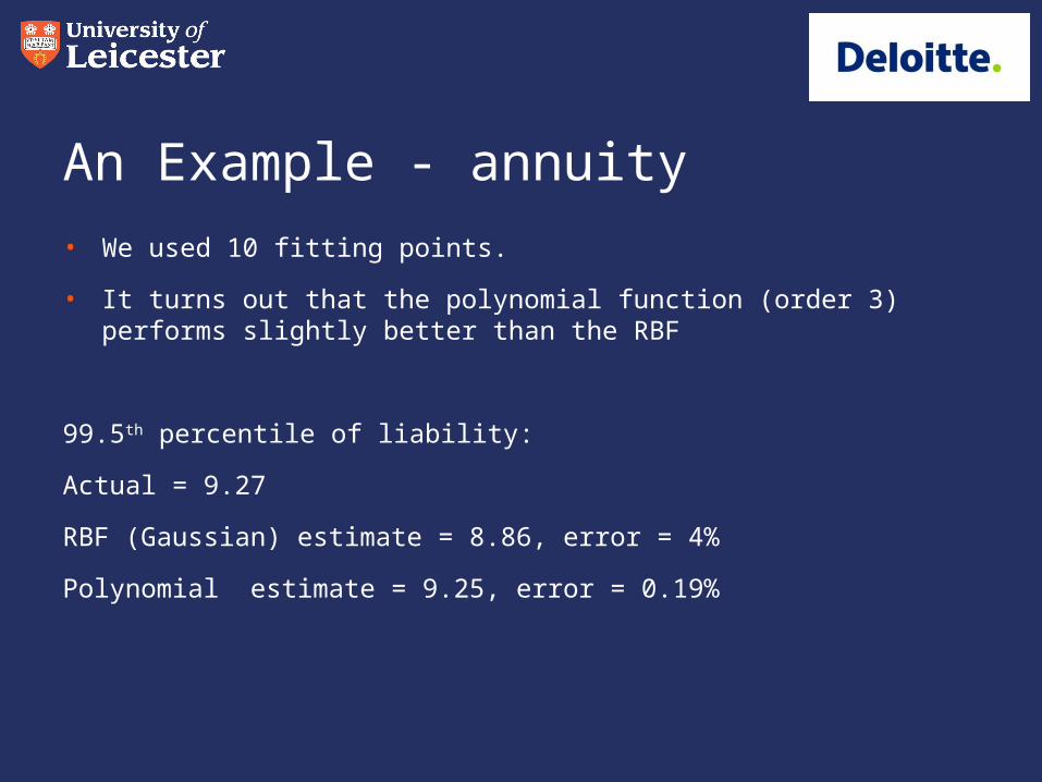
An Example - annuity• We used 10 fitting points.• It turns out that the polynomial function (order 3) performs slightly

better than the RBF

99.5th percentile of liability:Actual = 9.27RBF (Gaussian) estimate = 8.86, error = 4%Polynomial estimate = 9.25, error = 0.19%

Annuity – how good was the fit

What if there is a discontinuity?Chart shows liabilities against T, for fixed disc=8%: Was fitted using “norm” function.

Unlikely to arise in practice, though. However....

Choice of polynomial or RBF• Choice of appropriate polynomial terms is

problematic. High degree polynomials are famously unstable (Gibb’s phenomena)

• Choice of RBF is related to the “smoothness of the data” – see difference between Gaussian and norm function. This requires some user input, but does not require other experimentation.

• RBF is adaptable to the placement of new points near to where error is being observed in approximation. This is not robust with polynomial approximation.

With profits• The realistic balance sheet includes a “cost of guarantees”• For example, suppose there is a guaranteed sum assured on the assets, equal

to £500.• Crudely, we can model the cost of guarantees as a put option on the asset

share.Assume that:

Asset Share is £1,000Strike price (guarantee) is £500Assets ~ N (1000, 3002), disc~ N (8%, 2.5%2)

This time the radial basis function (“norm”) does better:

Actual = £83.53RBF estimate = £74.6, error = 11%Polynomial estimate = £1,735, error = 1978%

With profits Polynomial has difficulty coping with

the particular behaviour shown Also, the fitting problem is prone to

becoming singular RBF (using “norm”) does much better

Smoothing splines• If the data is noisy• Minimise

• Choice of l is crucial

gg

sysyfl YYYy

of measure smoothness)(

).())()(()( 2

l

freedom of degreesenough ifion interpolat ,squaresleast ,0

ll

Summary• It is worthwhile to explore the use of radial basis

functions for approximation.• They are good in high dimensions, and adapt

easily to the local shape of the surface. • Polynomials are good where the surface is close

to a polynomial in reality• They are also difficult to implement in high

dimensions.• There are different RBFs and different

approximation processes depending on the nature and reliability of the data.