Lecture Notes 3

Approximation Methods

In this chapter, we deal with a very important problem that we will encounter

in a wide variety of economic problems: approximation of functions. Such

a problem commonly occurs when it is too costly either in terms of time or

complexity to compute the true function or when this function is unknown

and we just need to have a rough idea of its main properties. Usually the only

thing that is required then is to be able to compute this function at one or a

few points and formulate a guess for all other values. This leaves us with some

choice concerning either the local or global character of the approximation

and the level of accuracy we want to achieve. As we will see in different

applications, choosing the method is often a matter of efficiency and ease of

computing.

Following Judd [1998], we will consider 3 types of approximation methods

1. Local approximation, which essentially exploits information on the value

of the function in one point and its derivatives at the same point. The

idea is then to obtain a (hopefully) good approximation of the function

in a neighborhood of the benchmark point.

2. Lp approximations, which actually find a nice function that is close to

the function we want to evaluate in the sense of a Lp norm. Ideally, we

would need information on the whole function to find a good approxi-

mation, which is usually infeasible – or which would make the problem

1

of approximation totally irrelevant! Therefore, we usually rely on inter-

polation, which then appears as the other side of the same problem, but

only requires to know the function at some points.

3. Regressions, which may be viewed as an intermediate situation between

the two preceding cases, as it usually relies — exactly as in econometrics,

on m moments to find n parameters of the approximating function.

3.1 Local approximations

The problem of the local approximation of a function f : R −→ R is to make

use of information about the function at a particular point x0 ∈ R, to produce

a good approximation of f in a neighborhood of x0. Among the various

available method 2 are of particular interest: the Taylor series expansion and

Pade approximation.

3.1.1 Taylor series expansion

Taylor series expansion is certainly the most wellknown and natural approxi-

mation to any student.

The basic framework: This approximation relies on the standard Taylor’s

theorem:

Theorem 1 Suppose F : R −→ R is a Ck+1 function, then for x? ∈ Rn, we

have

F (x) = F (x?) +n∑

i=1

∂F

∂xi(x?)(xi − x?i )

+1

2

n∑

i=1

n∑

i1=1

∂F

∂xi1∂xi2(x?)(xi1 − x?i1)(xi2 − x?i2) + . . .

+1

k!

n∑

i1=1

. . .n∑

ik=1

∂F

∂xi1 . . . ∂xi1(x?)(xi1 − x?i1) . . . (xik − x?ik)

+O

(‖x− x?‖k+1

)

2

The idea of Taylor expansion approximation is then to form a polynomial

approximation of the function f as described by the Taylor’s theorem. This

approximation method therefore applies to situations where the function is at

least n times differentiable to get a n–th order approximation. If this is the

case, then we are sure that the error will be at most of order O(‖x− x?‖k+1

).1.

In fact, we may look at Taylor series expansion from a slightly different

perspective and acknowledge that it amounts to approximate the function by

an infinite series. For instance in the one dimensional case, this amounts to

write

F (x) 'n∑

k=0

αk(x− x?)k

where αk = 1k!

∂F∂xi

(x?). As n tends toward infinity, the latter equation may be

understood as a power series expansion of the F in the neighborhood of x?.

This is a natural way to think of this type of approximation if we just think of

the exponential function for instance, and the way a computer delivers exp(x).

Indeed, the formal definition of the exponential function is traditionally given

by

exp(x) ≡∞∑

i=0

xk

k!

The advantage of this representation is that we are now in position to give

a very important theorem concerning the relevance of such approximation.

Nevertheless, we need to report some preliminary definitions.

Definition 1 We call the radius of convergence of the complex power series,

the quantity r defined by

r = sup

|x| :

∣∣∣∣∣

∞∑

k=0

αkxk

∣∣∣∣∣ <∞

r therefore provides the maximal radius of x ∈ C for which the complex series

converges. That is for any x ∈ C such that |x| < r, the series converges while

it diverges for any x ∈ C such that |x| > r.

1Let us recall at this point that a function f : Rn−→ Rk is O

(x`

)if limx→0

‖f(x)‖

‖x‖` < ∞

3

Definition 2 A function F : Ω ⊂ C −→ C is said to be analytic, if for every

x? ∈ Ω there exists a sequence αk and a radius r such that

F (x) =n∑

k=0

αk(x− x?)k for ‖x− x?‖ < r

Definition 3 Let F : Ω ⊂ C −→ C be a function, and x? ∈ Ω. x? is a

singularity of F is F is analytic on Ω− x? but not on Ω.

For example, let us consider the tangent function tan(x). tan(x) is defined by

the ratio of two analytic functions

tan(x) =sin(x)

cos(x)

since cos(x) and sin(x) may be written as

cos(x) =∞∑

i=0

(−1)n x2n

(2n)!

sin(x) =∞∑

i=0

(−1)n x2n+1

(2n+ 1)!

However, the function obviously admits a singularity at x? = π/2, for which

cos(x?) = 0.

Given these definition we can now enounce the following theorem:

Theorem 2 Let F be an analytic function in x ∈ C. If F or any derivative

of F exhibits a singularity at xo ∈ C, then the radius of convergence in the

complex plane of the Taylor series expansion of F in the neighborhood of x?

∞∑

k=0

1

k!

∂kF

∂xk(x?)(x− x?)k

is bounded from above by ‖x? − xo‖.

This theorem is extremely important as it gives us a guideline to use Taylor

series expansions, as it actually tells us that the series at x? cannot deliver

any accurate, and therefore reliable, approximation for F an any point farther

4

away from x? than any singular point of F . An extremely simple example

to understand this point is provided by the approximation of the function

F (x) = log(1− x), where x ∈ (−∞, 1), in a neighborhood of x? = 0. First of

all, note that xo = 1 is a singular value for F (x). The Taylor series expansion

of F (x) in the neighborhood of x? = 0 writes

log(1− x) ' ϕ(x) ≡ −∞∑

k=1

xk

k

What the theorem tells us is that this approximation may be used for values

of x such that ‖x − x?‖ is below ‖x? − xo‖ = ‖0 − 1‖ = 1, that is for x such

that −1 < x < 1. In other words, the radius of convergence of the Taylor

approximation to this function is r = 1. As an numerical illustration, we

report in table 3.1, the “true” value of log(1− x), its approximate value using

100 terms in the summation, and the absolute deviation of this approximation

from the “true” value.2 As can be seen from the table, as soon as ‖x? − xo‖approaches the radius, the accuracy of the approximation by the Taylor series

expansion performs more and more poorly.

Table 3.1: Taylor series expansion for log(1− x)

x log(1− x) ϕ100(x) ε

-0.9999 0.69309718 0.68817193 0.00492525-0.9900 0.68813464 0.68632282 0.00181182-0.9000 0.64185389 0.64185376 1.25155e-007-0.5000 0.40546511 0.40546511 1.11022e-0160.0000 0.00000000 0.00000000 00.5000 -0.69314718 -0.69314718 2.22045e-0160.9000 -2.30258509 -2.30258291 2.18735e-0060.9900 -4.60517019 -4.38945277 0.2157170.9999 -9.21034037 -5.17740221 4.03294

2The word true lies between quotes as it has been computed by the computer and istherefore an approximation!

5

The usefulness of the approach: This approach to approximation is par-

ticularly useful and quite widespread in economic dynamics. For instance,

anyone that has ever tried to study the dynamic properties of any macro

model — let’s say the optimal growth model — has once encountered the

method. Let’s take for instance the optimal growth model which dynamics

may be summarized — when preferences are logarithmic and technology is

Cobb–Douglas — by the two following equations3

kt+1 = kαt − ct + (1− δ)kt (3.1)1

ct= β

1

ct+1

(αkα−1t+1 + 1− δ

)(3.2)

It is a widespread practice to linearize of log–linearize such an economy around

the steady state, which we will define later on, to study the local dynamic

properties of the equilibrium. Let’s assume that the steady state has already

been found and is given by ct+1 = ct = c? and kt+1 = kt = k? for all t.

Linearization: let us denote by kt the deviation of the capital stock kt with

respect to its steady state level in period t, such that kt = kt − k?. Likewise,

we define ct = ct− c?. The first step of linearization is to reexpress the system

in terms of functions. Here, we can define

F (kt+1, ct+1, kt, ct) =

kt+1 − kαt + ct − (1− δ)kt

1ct− β 1

ct+1

(αkα−1t+1 + 1− δ

)

and then build the Taylor expansion

F (kt+1, ct+1, kt, ct) ' F (k?, c?, k?, c?) + F1(k?, c?, k?, c?)kt+1 + F2(k

?, c?, k?, c?)ct+1

+F3(k?, c?, k?, c?)kt + F4(k

?, c?, k?, c?)ct

3Since we just want to make the case of Taylor series expansions, we do not need to beany more precise on the origin of these two equations. Therefore, we will take them as given,but we will come back to their determination in the sequel.

6

We therefore just have to compute the derivatives of each sub–function, and

realize that the steady state corresponds to a situation where F (k?, c?, k?, c?) =

0. This yields the following system

kt+1 − αk?α−1kt + ct − (1− δ)kt = 0

− 1c?2 ct + β 1

c?2

(αk?α−1 + 1− δ

)ct+1 − β 1c?α(α− 1)k?α−2kt+1 = 0

which simplifies to

kt+1 − αk?α−1kt + ct − (1− δ)kt = 0

−ct + β(αk?α−1 + 1− δ

)ct+1 − βα(α− 1) c

?

k?k?α−1kt+1 = 0

We then have to solve the implied linear dynamic system, bu this is another

story that we will deal with in a couple of chapters.

Log–linearization: Another common practice is to take a log–linear ap-

proximation to the equilibrium. Such an approximation is usually taken be-

cause it delivers a natural interpretation of the coefficients in front of the

variables: these can be interpreted as elasticities. Indeed, let’s consider the

following one–dimensional function f(x) and let’s assume that we want to take

a log–linear approximation of f around x?. This would amount to have, as

deviation, a log–deviation rather than a simple deviation, such that we can

define

x = log(x)− log(x?)

Then, a restatement of the problem is in order, as we are to take an approxi-

mation with respect to log(x):

f(x) = f(exp(log(x)))

which leads to the following first order Taylor expansion

f(x) ' f(x?) + f ′(exp(log(x?))) exp(log(x?))x = f(x?) + f ′(x?)x?x

If we apply this technic to the growth model, we end up with the following

system

kt+1 − 1−β(1−δ)β kt +

(1−β(1−δ)

αβ − δ)ct − (1− δ)kt = 0

−ct + ct+1 − (α− 1)(1− β(1− δ))kt+1 = 0

7

3.2 Regressions as approximation

This type of approximation is particularly common in economics as it just cor-

responds to ordinary least square (OLS) . As you know the problem essentially

amounts to approximate a function F by another function G of exogenous vari-

ables. In other words, we have a set of observable endogenous variables yi,

i = 1 . . . N , which we are willing to explain in terms of the set of exogenous

variables Xi = x1i , . . . , xki , i = 1 . . . N . This problem amounts to find a set

of parameters Θ that solves the problem

minΘ∈Rp

N∑

i=1

(yi −G(Xi; Θ))2 (3.3)

The idea is therefore that Θ is chosen such that on average G(X ; Θ) is close

enough to y, such that G delivers a “good” approximation for the true function

F in the region of x that we consider. This is actually nothing else than

econometrics!

There are however several choices that can be made and that give us much

more freedom than in econometrics. We now consider investigate these choices.

Number of data points: Econometricians never have the choice of the

points they can use to reveal information on the F function, as data are given

by history. In numerical analysis this constraint is relaxed, we may be exactly

identified for example, meaning that the number of data points, N , is exactly

equal to the number of parameters, p, we want to reveal. Never would a good

econometrician do this kind of thing! Obviously, we can impose a situation

where N > p in order to exploit more information. The difference between

these two choices should be clear to you, in the first case we are sure that

the approximation will be exact in the selected points, whereas this will not

necessarily be the case in the second experiment. To see that, just think of the

following: assume we have a sample made of 2 data points for a function that

we want to approximate using a linear function. we actually need 2 parameters

8

to define a linear function: the intercept, α and the slope β. In such a case,

(3.3) rewrites

minα,β

(y1 − α− βx1)2 + (y2 − α− βx2)

2

which yields the system of orthogonality conditions

(y1 − α− βx1) + (y2 − α− βx2) = 0

(y1 − α− βx1)x1 + (y2 − α− βx2)x2 = 0

which rewrites(

1 1x1 x2

)(y1 − α− βx1y2 − α− βx2

)≡ A.v = 0

This system then just amounts to find the null space of the matrix A, which,

in the case x1 6= x2 (which we can always impose as we will see next), imposes

vi = 0, i = 1, 2. This therefore leads to

y1 = α+ βx1

y2 = α+ βx2

such that the approximation is exact. When the system is overidentified this

is not the case anymore.

Selection of data points: This is actually a major difference between

econometrics and numerical approximations. We do control the space over

which we want to take an approximation. In particular, we can spread the

data points wherever we want in order to control information. For instance,

let us consider the particular case of the function depicted in figure (3.1). As

this function exhibits a kink in x? it may be beneficial to concentrate a lot

of points around x? in order to reveal as much information as possible on the

kink.

Functional forms: One key issue in the selection of the approximating

function is a functional form. In most of the cases, a sequence of monomials

9

Figure 3.1: Selection of points

6

-x

y = F (x)

x?

of different degrees is selected: Xi = 1, xi, x2, . . . , xp, One advantage of this

selection is basically simplicity. However, this often turns to be a very bad

choice as many problems then turn out to be ill–conditioned with such a choice.

The most obvious objection we may formulate against this specification choice

is related to the multicolinearity problem. Assume for instance that you want

to approximate a production function that depends on employment and the

capital stock. The capital stock is basically an extremely smooth variable

as, by construction, it is essentially a smooth moving average of investment

decisions

kt+1 = it + (1− δ)kt ⇐⇒ kt+1 =∞∑

`=0

(1− δ)`it−`

Therefore, taking as a basis for exogenous variables powers of the capital stock

is basically a bad idea. To see that, let us assume that δ = 0.025 and it is a

white noise process with volatility 0.1, then let us simulate a 1000 data points

process for the capital stock and let us compute the correlation matrix for kjt ,

10

j = 1, . . . , 4, we get:

kt k2t k3t k4tkt 1.0000 0.9835 0.9572 0.9315k2t 0.9835 1.0000 0.9933 0.9801k3t 0.9572 0.9933 1.0000 0.9963k4t 0.9315 0.9801 0.9963 1.0000

implying a very high correlation between the powers of the capital stock, there-

fore raising the possibility of occurrence of multicolinearity. A typical answer

to this problem is to rely on orthogonal polynomials rather than monomials.

We will discuss this issue extensively in the next section. A second possibility is

to rely on parcimonious approaches that do not require too much information

in terms of function specification. An alternative is to use neural networks.

Before going to Neural Network approximations, we first have to deal with

a potential problem you may face with all the examples I gave is that when

we solve a model: the true decision rule is unknown, such that we do not

know the function we are dealing with. However, the main properties of the

decision rule are known, in particular, we know that it has to satisfy some

conditions imposed by economic theory. As an example, let us attempt to find

an approximate solution for the consumption decision rule in the deterministic

optimal growth model. Economic theory teaches us that consumption should

satisfy the Euler equation

c−σt = βc−σt+1(αkα−1t+1 + 1− δ

)(3.4)

knowing that the capital stock evolves as

kt+1 = kαt − ct + (1− δ)kt (3.5)

Let us assume that consumption may be approximated by

φ(kt, θ) = exp(θ0 + θ1 log(kt) + θ2 log(kt)

2)

over the interval [k; k]. Our problem is then to find the triple θ0, θ1, θ2 suchthat

N∑

t=1

[φ(kt, θ)

−σ − βφ(kt+1, θ)−σ(αkα−1t+1 + 1− δ

)]2

11

is minimum. This actually amounts to solve a non–linear least squares prob-

lem. However, a lot of structure is put on this problem as kt+1 has to satisfy

the law of motion for capital:

kt+1 = kαt − exp(θ0 + θ1 log(kt) + θ2 log(kt)

2)+ (1− δ)kt

The algorithm then works as follows

1. Set a grid ofN data points, kiNi=1, for the capital stock over the interval

[k; k], and an initial vector θ0, θ1, θ2.

2. for each ki, i = 1, . . . , N , and given θ0, θ1, θ2, compute

ct = φ(kt, θ)

and

kt+1 = kαt − φ(kt, θ) + (1− δ)kt

3. Compute

ct+1 = φ(kt+1, θ)

and the quantity

R(kt, θ) ≡ φ(kt, θ)−σ − βφ(kt+1, θ)

−σ(αkα−1t+1 + 1− δ

)

4. If the quantityN∑

t=1

R(ki, θ)2

is minimal then stop, else update θ0, θ1, θ2 and go back to 2.

As an example, I computed the approximate decision rule for the deterministic

optimal growth model with α = 0.3, β = 0.95, δ = 0.1 and σ = 1.5. I consider

that the model may deviate up to 90% from its capital stock steady state —

k = 0.1k? and k = 1.9k? — and used 20 data points. Figure 3.2 reports the

approximate decision rule versus the “true” decision rule.4 As can be seen

4The “true” decision rule was computed using value iteration, which we shall study later.

12

from the graph, the solution we obtained with our approximation is rather

accurate and we actually have

1

N

N∑

i=1

∣∣∣∣ctruei − cLSi

ctruei

∣∣∣∣ = 8.743369e−4 and maxi=1,...,N

∣∣∣∣ctruei − cLSi

ctruei

∣∣∣∣ = 0.005140

such that the error we are making is particularly small. Indeed, using the

approximate decision rule, an agent would make a maximal error of 0.51% in

its economic calculus — i.e. 51 cents for each 100$ spent on consumption.

Figure 3.2: Least–square approximation of consumption

0 0.5 1 1.5 2 2.5 3 3.5 4 4.5 50.4

0.6

0.8

1

1.2

1.4

1.6

1.8

Capital stock

Con

sum

ptio

n

True Decision RuleLS approximation

A neural network may be simply viewed as a particular type of function,

which are flexible enough to fit fairly general functions. A neural network may

be simply understood using the standard metaphor of human brain. There is

an input, x, which is processed by a node. Each node is actually a function that

transforms the input into an output which is then itself passed to another node.

For instance, panel (a) of figure 3.3, borrowed from Judd [1998], illustrates the

13

single–layer neural network whose functional form is

G(x, θ) = h

(n∑

i=1

θig(x(i))

)

where x is the vector of inputs, and h and g are scalar functions. A common

choice for g in the case of the dingle layer neural network is g(x) = x. There-

fore, if we set h to be identity too, we are back to the standard OLS model

with monomials. A second a perhaps much more interesting type of neural

Figure 3.3: Neural Networks

(a) (b)

x1

x2

xn

........

~q>

- y

x1

x2

xn

........

q

R

U

1q

w:µ

¸s-3

- y

network is depicted in panel (b) of figure 3.3. This type of neural network

is called the hidden–layer feedforward network. In this specification, we are

closer to the idea of network as the transformed input is fed to another node

that process it to get information. The associated function form is given by

G(x, θ, γ) = f

m∑

j=1

γjh

(n∑

i=1

θji g(x(i))

)

In this case, h is called the hidden–layer activation function. h should be a

“squasher” function — i.e. a monotically nondecreasing function that maps

R onto [0; 1]. Three very popular functions are

1. The heaviside step function

h(x) =

1 for x > 00 for x < 0

14

2. The sigmoid function

h(x) =1

1 + exp(−x)

3. Cumulative distribution functions, for example the normal cdf

h(x) =1√2πσ

∫ x

−∞exp

(− x2

2σ2

)

Obtaining an approximation then simply amounts to determine the set

of coefficients γj , θji ; i = 1 . . . n, j = 1, . . . ,m. This can be simply achieved

running non–linear least squares, that is solving

minθ,γ

N∑

`=1

(y` −G(x`, θ, γ))2

One particular nice feature of neural networks is that they deliver accurate

approximation using only few parameters. This characteristic is related to the

high flexibility of the approximating functions they use. Further, as established

by the following theorem by Hornik, Stinchcombe and White [1989], neural

network are extremely powerful in that they offer a universal approximation

method.

Theorem 3 Let f : Rn −→ R be a continuous function to be approximated.

Let h be a continuous function, h : R → R, such that either (i)∫∞−∞ h(x)dx

is finite and non zero and h is Lp for 1 6 p 6 ∞ or (ii) h is a “squashing”

function (nondecreasing, limx→∞ h(x) = 1,limx→−∞ h(x) = 0). Let

Σn(h) =

g : Rn → R, g(x) =

n∑

j=1

θjh(wj .x+ aj),

aj , θj ∈ R, and wj ∈ Rn, wj 6= 0,m = 1, 2, . . .

be the set of all possible single hidden–layer feedforward neural networks, using

h as the hidden layer activation function. Then, for all ε > 0, probability

measure µ, and compact sets K ⊂ Rn, there is a g ∈ Σ(h) such that

supx∈K

|f(x)− g(x)| 6 ε and

∫

K|f(x)− g(x)|dµ 6 ε

15

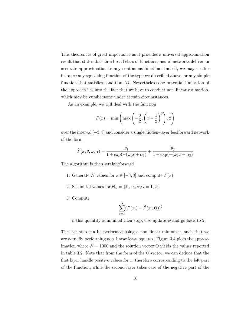
This theorem is of great importance as it provides a universal approximation

result that states that for a broad class of functions, neural networks deliver an

accurate approximation to any continuous function. Indeed, we may use for

instance any squashing function of the type we described above, or any simple

function that satisfies condition (i). Nevertheless one potential limitation of

the approach lies into the fact that we have to conduct non–linear estimation,

which may be cumbersome under certain circumstances.

As an example, we will deal with the function

F (x) = min

(max

(−3

2,

(x− 1

2

)3), 2

)

over the interval [−3; 3] and consider a single hidden–layer feedforward network

of the form

F (x, θ, ω, α) =θ1

1 + exp(−(ω1x+ α1)+

θ21 + exp(−(ω2x+ α2)

The algorithm is then straightforward

1. Generate N values for x ∈ [−3; 3] and compute F (x)

2. Set initial values for Θ0 = θi, ωi, αi; i = 1, 2

3. ComputeN∑

i=1

(F (xi)− F (xi,Θ))2

if this quantity is minimal then stop, else update Θ and go back to 2.

The last step can be performed using a non–linear minimizer, such that we

are actually performing non–linear least–squares. Figure 3.4 plots the approx-

imation where N = 1000 and the solution vector Θ yields the values reported

in table 3.2. Note that from the form of the Θ vector, we can deduce that the

first layer handle positive values for x, therefore corresponding to the left part

of the function, while the second layer takes care of the negative part of the

16

Table 3.2: Neural Network approximation

θ1 ω1 α1 θ2 ω2 α22.0277 6.8424 -10.0893 -1.5091 -7.6414 -2.9238

function. Further, it appears that the function is no so badly approximated

by this simple neural network, as

E2 =1

N

(N∑

i=1

(F (xi)− F (xi, Θ)2

) 12

= 0.0469

and

E∞ = maxi

∣∣∣F (xi)− F (xi, Θ)∣∣∣ = 0.2200

Figure 3.4: Neural Network Approximation

−3 −2 −1 0 1 2 3−2

−1.5

−1

−0.5

0

0.5

1

1.5

2

2.5

x

True Neural Network

All these methods actually relied on regressions. They are simple, but

may be either totally unreliable and ill–conditioned in a number of problem, or

17

difficult to compute because they rely on non–linear optimization. We will now

consider methods which will actually be more powerful and somehow simpler

to implement. They however require introducing some important preliminary

concepts, among which that of orthogonal polynomials

3.2.1 Orthogonal polynomials

This class of polynomial possesses — by definition — the orthogonality prop-

erty which will prove to be extremely efficient and useful in a number of

problem. For instance, this will solve the multicolinearity problem we encoun-

tered in OLS. This property will also greatly simplify the computation of the

approximation in a number of problems we will deal with in the sequel. First

of all we need to introduce some preliminary concepts.

Definition 4 (Weighting function) A weighting function ω(x) on the in-

terval [a; b] is a function that is positive almost everywhere on [a; b] and has a

finite integral on [a; b].

An example of such a weighting function is ω(x) = (1−x)−1/2 over the interval[-1;1]. Indeed, limx→−1 ω(x) =

√2/2, and ω′(x) > 0 such that ω(x) is positive

everywhere over the whole interval. Further

∫ 1

−1(1− x2)−1/2dx = arcsin(x)

∣∣∣∣1

−1

= π

Definition 5 (Inner product) Let us consider two functions f1(x) and f2(x)

both defined at least on [a; b], the inner product with respect to the weighting

function ω(x) is given by

〈f1, f2〉 =∫ b

af1(x)f2(x)ω(x)dx

For example, assume that f1(x) = 1, f2(x) = x and ω(x) = (1 − x2)( − 1/2),

then the inner product over the interval [-1;1] is

〈f1, f2〉 =∫ 1

−1

x√1− x

dx = −√

1− x2∣∣∣∣1

−1

= 0

18

Hence, in this case, we have that the inner product of 1 and x with respect

to ω(w) on the interval [-1;1] is identically null. This will actually define the

orthogonality property.

Definition 6 (Orthogonal Polynomials) The family of polynomials Pn(x)is mutually orthogonal with respect to ω(x) iff

〈Pi, Pj〉 = 0 for i 6= j

Definition 7 (Orthonormal Polynomials) The family of polynomials Pn(x)is mutually orthonormal with respect to ω(x) iff it is orthogonal and

〈Pi, Pi〉 = 1 for all i

Table 3.3 reports the most common families of orthogonal polynomials (see

Judd [1998] for a more detailed exposition) and table 3.4 their recursive for-

mulation

Table 3.3: Orthogonal polynomials (definitions)

Family ω(x) [a; b] Definition

Legendre 1 [−1; 1] Pn(x) =(−1)n

2nn!dn

dxn (1− x2)n

Chebychev (1− x2)−1/2 [−1; 1] Tn(x) = cos(n cos−1(x))

Laguerre exp(−x) [0,∞) Ln(x) =exp(x)n!

dn

dxn (xn exp(−x))

Hermite exp(−x2) (−∞,∞) Hn(x) = (−1)n exp(x2) dndxn exp(−x2)

3.3 Least square orthogonal polynomial approxima-

tion

We will now discuss one of the most common approach to approximation that

goes back to the easy OLS approach we have seen previously.

19

Table 3.4: Orthogonal polynomials (recursive representation)

Family 0 1 Recursion

Legendre P0(x) = 1 P1(x) = x Pn+1(x) =2n+1n+1 xPn(x)− n

n+1Pn−1(x)

Chebychev T0(x) = 1 T1(x) = x Tn+1(x) = 2xTn(x)− Tn−1(x)

Laguerre L0(x) = 1 L1(x) = 1− x Ln+1(x) =2n+1−xn+1 Ln(x)− n

n+1Ln−1(x)

Hermite H0(x) = 1 H1(x) = 2x Hn+1(x) = 2xHn(x)− 2nHn−1(x)

Definition 8 Let F : [a, b] −→ R be a function we want to approximate,

and g(x) a polynomial approximation of F . The least square polynomial ap-

proximation of F with respect to the weighting function ω(w) is the degree n

polynomial that solves

mindeg(g)6n

∫ b

a(F (x)− g(x))2 ω(x)dx

This equation may be understood adopting an econometric point of view,

as ω(w) may be given a weighting matrix interpretation we find in GMM

estimation. Indeed, ω(x) furnishes an indication on how much we care about

approximation errors as a function of x. Therefore, setting ω(x) = 1, which

amounts to put the same weight on any x then corresponds to a simple OLS

approximation.

Let us now assume that g(x) =∑n

i=0 ciϕi(x), where ϕk(x)nk=0 is a se-

quence of orthogonal polynomials, the least square problem rewrites

mincini=0

∫ b

a

(F (x)−

n∑

i=0

ciϕi(x))

)2ω(x)dx

for which the first order conditions are given by

∫ b

a

(F (x)−

n∑

i=0

ciϕi(x))

)ϕi(x)ω(x)dx = 0 for i = 0, . . . , n

20

which yields

ci =〈F,ϕi〉〈ϕi, ϕi〉

Therefore, we have

F (x) 'n∑

i=0

〈F,ϕi〉〈ϕi, ϕi〉

ϕi(x)

There are several examples of the use of this type of approximation. Fourier

approximation is an example of those which is suitable for periodic functions.

Nevertheless, I will focus in a coming section on one particular approach, which

we will use quite often in the next chapters: Chebychev approximation.

Beyond least square approximation, there exists other approaches that

departs from the least square by the norm they use:

• Uniform approximation, which attempt to solve

limn→∞

maxx∈[a;b]

|F (x)− pn(x)| = 0

The main difference between this approach and L2 approximation is that

contrary to L2 norms that put no restrictions on the approximation on

particular points, the uniform approximation imposes that the approxi-

mation of F at each x is exact, whereas L2 approximations juste requires

the total error to be as small as possible.

• Minimax approximations, which rest on the L∞ norm, such that these

approximations attempt to find an approximation that provides the best

uniform approximation to the function F that is we search the degree n

polynomial that achieves

mindeg(g)6n

‖F (x)− g(x)‖∞

There are theorems in approximation theory that states that the quality

of this approximation increases polynomially as the degree of polyno-

mials increases, and the polynomial rate of convergence is faster for

21

smoother functions. Nevertheless, if this approximation can be as good

as needed for F , no use of its derivatives is made, such that the deriva-

tives may be very poorly approximated. Finally, such approximation

methods are extremely difficult to compute.

3.4 Interpolation methods

Up to now, we have seen that there exist methods to compute the value of a

function at some particular points, but in most of the cases we are not only

interested by the function at some points but also between these points. This

is the problem of interpolation.

3.4.1 Linear interpolation

This method is totally straightforward and known to everybody. Assume you

have a collection of data points C = (xi, yi)|i = 1, . . . , n. Then for any

x ∈ [xi−1, xi], we can compute y as

y =yi − yi−1xi − xi−1

x+xiyi−1 − xi−1yi

xi − xi−1

Although, such approximations have proved to be very useful in a lot of ap-

plications, it can be particularly inefficient for different reasons:

1. It does not deliver an approximating function but rather a collection of

approximations for each interval;

2. it requires to identify the interval where the approximation is to be

computed, which may be particularly costly when the interval is not

uniform;

3. it can obviously perform very badly for non–linear functions.

Therefore, there obviously exist alternative interpolation methods that per-

form better, but which are not necessarily more efficient.

22

3.4.2 Lagrange interpolation

This type of approximation is quite demanding as it consider a collection of

data C = (xi, yi)|i = 1, . . . , n with distinct xi — called the Lagrange data.

Lagrange interpolation amounts to find a degree n− 1 polynomial P (x), such

that yi = P (xi). Therefore, the method is exact for each point. Lagrange

interpolating polynomials are defined by

Pi(x) =∏

j 6=i

x− xjxi − xj

Note that Pi(xi) = 1 and Pi(xj) = 0. The interpolation is then given by

P (x) =n∑

i=1

yiPi(x)

The obvious problem that we can immediately see from this formula is that

if the number of point is high enough, this type of interpolation is totally

untractable. Indeed, just to compute a single Pi(x) this already requires 2(n−1) substractions, n multiplications. Then this has to be constructed for the

n data points to compute all needed Pi(x). Then to compute P (x) we need

n additions and n multiplications. Therefore, this requires 3n2 operations!

Therefore, one actually may actually attempt to compute directly:

P (x) =n−1∑

i=0

αixi

which may be obtained by solving the linear system

y1 = α0 + α1x1 + α2x21 + . . .+ αn−1x

n−11

y2 = α0 + α1x2 + α2x22 + . . .+ αn−1x

n−12

...yn = α0 + α1xn + α2x

2n + . . .+ αn−1x

n−1n

or

Aα = y

23

where α = α0, α1, . . . , αn−1′ and A is the so–called Vandermonde matrix for

xi, i = 1, . . . , n

A =

1 x1 x21 · · · xn−11

1 x2 x22 · · · xn−12...

......

. . ....

1 xn x2n · · · xn−1n

If the Lagrange formula guarantees the existence of the interpolation, the

following theorem guarantees its uniqueness.

Theorem 4 Provided the interpolating points are distincts, there is a unique

solution to the Lagrange interpolation problem.

The proof of the theorem may be sketched as follows. Assume that besides

P (x), there exists another interpolating polynomial P ?(x) of degree at most

n− 1 that also interpolates the n data points. Then, by construction, P (x)−P ?(x) is at most of degree n − 1 and is zeros at all n nodes. But the only

polynomial of degree n − 1 that has n zeros is 0, such that P (x) = P ?(x).

Here again, the method may be quite demanding from a computational point of

view, as we have to invert a matrix of size (n×n). There then exist much more

efficient methods, and in particular the so–called Chebychev approximation

that works very well for smooth functions.

3.5 Chebychev approximation

Chebychev approximation uses . . . Chebychev polynomials as a basis for the

polynomials (see figure 3.5). These polynomials are described by the recursion

Tn+1(x) = 2xTn(x)− Tn−1(x) with T0(x) = 1, T1(x) = x

which admits as solution

Tn(x) = cos(n cos−1(x))

as aforementioned these polynomials form an orthogonal basis with respect to

the weighting function ω(x) = (1−x2)−1/2 over the interval [−1; 1]. Neverthe-

less, this interval may be generalized to [a; b], by transforming the data using

24

the formula

x = 2y − a

b− a− 1 for y ∈ [a; b]

Beyond the standard orthogonality property, Chebychev polynomials exhibit

a discrete orthogonality property which writes as

n∑

i=1

Ti(rk)Tj(rk) =

0 for i 6= jn for i = j = 0n2 for i = j 6= 0

where rk, k = 1, . . . , n are the roots of Tn(x) = 0.

Figure 3.5: Chebychev polynomials

−1 −0.8 −0.6 −0.4 −0.2 0 0.2 0.4 0.6 0.8 1−1

−0.8

−0.6

−0.4

−0.2

0

0.2

0.4

0.6

0.8

1

x

n=1n=2n=3n=4

A first theorem will state the usefulness of Chebychev approximation.

Theorem 5 Assume F is a Ck function over the interval [−1; 1], and let

ci =2

π

∫ 1

−1

F (x)Ti(x)√1− x2

dx for i = 0 . . . n

and

gn(x) ≡c02

+n∑

i=1

ciTi(x)

25

Then, there exists ε <∞ such that for all n > 2

‖F (x)− gn(x)‖∞ 6 εlog(n)

nk

This theorem is of great importance as it actually states that the approx-

imation gn(x) will be as close as we might want to F (x) as the degree of

approximation n increases to ∞. In effect, since the approximation error is

bounded by above by ε log(n)nk

and since the latter expression tends to zero

as n tends toward ∞, we have that gn(x) converges uniformly to F (x) as n

increases. Further, the next theorem will establish a useful property on the

coefficients of the approximation.

Theorem 6 Assume F is a Ck function over the interval [−1; 1], and admitsa Chebychev representation

F (x) =c02

+∞∑

i=1

ciTi(x)

then, there exists c such that

|ci| 6c

ikfor j > 1

This theorem is particularly important as it states that the smoother the

function to be approximated is (the greater k is), the faster is the pace at

which coefficients will drop off. In other words, we will be able to achieve a

high enough accuracy using less coefficients.

At this point, we have established that Chebychev approximation can be

accurate for smooth functions, but we still do not know how to proceed to get

a good approximation. In particular, a very important issue is the selection

of interpolating data points, the so–called nodes. This is the main problem

of interpolation: how to select nodes such that we minimize the interpolation

error? The answer to this question is particularly simple in the case of Cheby-

chev interpolation: the nodes should be the zeros of the nth degree Chebychev

polynomial.

26

We are then endowed with data points to compute the approximation.

Using m > n data points, we can compute the (n − 1)th order Chebychev

approximation relying on the Chebychev regression algorithm we will now

describe in details. When m = n, the algorithm reduces to the so–called

Cebychev interpolation formula. Let us consider the following problem: Let

F : [a; b] −→ R, let us construct a degree n 6 m polynomial approximation of

F on [a; b]:

G(x) ≡n∑

i=0

αiTi

(2x− a

b− a− 1

)

1. Compute m > n + 1 Chebychev interpolation nodes on [−1; 1], whichare the roots of the degree m Chebychev polynomial

rk = −cos(2k − 1

2mπ

)for k = 1 . . . ,m

2. Adjust the nodes, rk, to fit in the [a; b] interval

xk = (rk + 1)b− a

2+ a for k = 1 . . . ,m

3. Evaluate the function F at each approximation node xk, to get a collec-

tion of ordinates

yk = F (xk) for k = 1 . . . ,m

4. Compute the collection of n+ 1 coefficients α = αi; i = 0 . . . n as

αi =

m∑

k=1

ykTi(rk)

m∑

k=1

Ti(rk)2

5. Form the approximation

G(x) ≡n∑

i=0

αiTi

(2x− a

b− a− 1

)

27

Note that step 4 actually can be interpreted in terms of an OLS problem as

— because of the orthogonality property of the Chebychev polynomials — αi

is given by

αi =cov(y, Ti(x))

var(Ti(x))

which may be recast in matricial notations as

α = (X ′X)−1X ′Y

where

X =

T0(x1) T1(x1) · · · Tn(x1)T0(x2) T1(x2) · · · Tn(x2)

......

. . ....

T0(xm) T1(xm) · · · Tn(xm)

and Y =

y1y2...ym

We now report two examples implementing the algorithm. The first one

deals with a smooth function of the type F (x) = xθ. The second one evalu-

ate the accuracy of the approximation in the case of a non–smooth function:

F (x) = min(max(−1.5, (x− 1/2)3), 2).

In the case of the smooth function, we set θ = 0.1 and approximate the

function over the interval [0.01; 2]. We select 100 nodes and evaluate the

accuracy of degree 2 and 6 approximation. Figure 3.6 reports the true function

and the corresponding approximation, table 3.5 reports the coefficients. As

can be seen from the table, adding terms in the approximation does not alter

the coefficients of lower degree. This just reflects the orthogonality properties

of the Chebychev polynomials, that we saw in the formula determining each

αi. This is of great importance, as it states that once we have obtained a high

order approximation, obtaining lower orders is particularly simple. This is

the economization principle. Further, as can be seen from the figure, a “good

approximation” to the function is obtained at rather low degrees. Indeed, the

difference between the function and its approximation at order 6 is already

good.

28

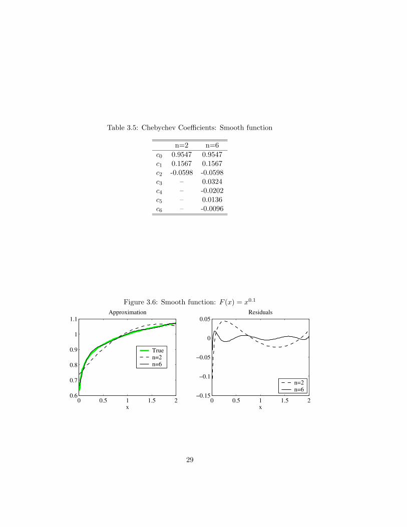
Table 3.5: Chebychev Coefficients: Smooth function

n=2 n=6

c0 0.9547 0.9547c1 0.1567 0.1567c2 -0.0598 -0.0598c3 – 0.0324c4 – -0.0202c5 – 0.0136c6 – -0.0096

Figure 3.6: Smooth function: F (x) = x0.1

0 0.5 1 1.5 20.6

0.7

0.8

0.9

1

1.1

x

Approximation

Truen=2 n=6

0 0.5 1 1.5 2−0.15

−0.1

−0.05

0

0.05

x

Residuals

n=2n=6

29

Matlab Code: Smooth Function Approximation

m = 100; % number of nodes

n = 6; % degree of polynomials

rk = -cos((2*[1:m]-1)*pi/(2*m)); % Roots of degree m polynomials

a = 0.01; % lower bound of interval

b = 2; % upper bound of interval

xk = (rk+1)*(b-a)/2+a; % nodes

Y = xk.^0.1; % compute the function at nodes

%

% Builds Chebychev polynomials

%

Tx = zeros(m,n+1);

Tx(:,1) = ones(m,1);

Tx(:,2) = xk(:);

for i=3:n+1;

Tx(:,i) = 2*xk(:).*Tx(:,i-1)-Tx(:,i-2);

end

%

% Chebychev regression

%

alpha = X\Y; % compute the approximation coefficients

G = X*a; % compute the approximation

In the case of the non–smooth function we consider (F (x) = min(max(−1.5, (x−1/2)3), 2)), the coefficients remain large even at degree 15 and the residuals

remain high at order 15. This actually indicates that Chebychev approxima-

tions are well suited for smooth functions, but have more difficulties to capture

kinks. Nevertheless, increasing the order of the approximation drastically, we

can achieve a much better approximation.

In the later case, it seems that a piecewise approximation would perform

better. Indeed, in this case, we may compute 3 approximation

• for x ∈ (−∞, x), G(x) = −1.5

• for x ∈ (x, x), G(x) ≡∑ni=0 βiTi

(2x−ab−a − 1

)

• for x ∈ (x,∞), G(x) = 2

where x is such that

(x− 1/2)3 = −1.5

30

Table 3.6: Chebychev Coefficients: Non–smooth function

n=3 n=7 n=15

c0 -0.0140 -0.0140 -0.0140c1 2.0549 2.0549 2.0549c2 0.4176 0.4176 0.4176c3 -0.3120 -0.3120 -0.3120c4 – -0.1607 -0.1607c5 – -0.0425 -0.0425c6 – -0.0802 -0.0802c7 – 0.0571 0.0571c8 – – 0.1828c9 – – 0.0275c10 – – -0.1444c11 – – -0.0686c12 – – 0.0548c13 – – 0.0355c14 – – -0.0012c15 – – 0.0208

Figure 3.7: Non–smooth function: F (x) = min(max(−1.5, (x− 1/2)3), 2)

−4 −2 0 2 4−2

−1

0

1

2

3

x

Approximation

Truen=3 n=7 n=15

−4 −2 0 2 4−0.5

0

0.5

1

x

Residuals

n=3 n=7 n=15

31

and x satisfies

(x− 1/2)3 = 2

In such a case, the approximation would be perfect with n = 3. This suggests

that piecewise approximation may be of interest in a number of cases.

3.6 Piecewise interpolation

We have actually already seen piecewise approximation method: the linear

interpolation method. But there exist more powerful and efficient method that

use splines. A spline can be any smooth function that is piecewise polynomial,

but most of all it should be smooth at all nodes.

Definition 9 A function S(x) on an interval [a; b] is a spline of order n if

1. S(x) is a C n−2 function on [a; b],

2. There exist a collection of ordered nodes a = x0 < x1 < . . . < xm = b

such that S(x) is a polynomial of order n− 1 on each interval [xi;xi+1],

i = 0, . . . ,m− 1

Examples of spline functions are

• Cubic splines: These splines functions are splines of order 4. These

splines are the most popular and are of the form

Si(x) = ai + bi(x− xi) + ci(x− xi)2 + di(x− xi)

3 for x ∈ [xi;xi+1]

• B0–splines: These functions are splines of order 1:

B0i (x) =

0, x < xi1, xi 6 x 6 xi+10, x > xi+1

32

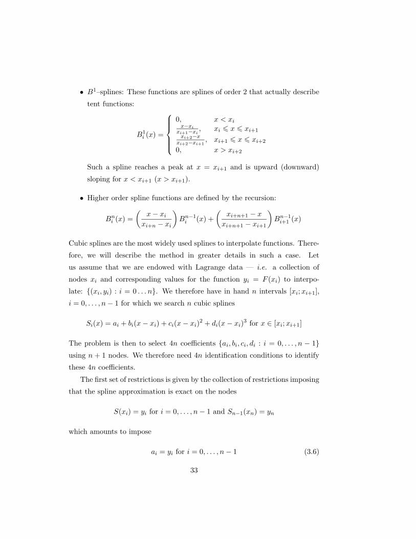
• B1–splines: These functions are splines of order 2 that actually describe

tent functions:

B1i (x) =

0, x < xix−xi

xi+1−xi, xi 6 x 6 xi+1

xi+2−xxi+2−xi+1

, xi+1 6 x 6 xi+2

0, x > xi+2

Such a spline reaches a peak at x = xi+1 and is upward (downward)

sloping for x < xi+1 (x > xi+1).

• Higher order spline functions are defined by the recursion:

Bni (x) =

(x− xi

xi+n − xi

)Bn−1i (x) +

(xi+n+1 − x

xi+n+1 − xi+1

)Bn−1i+1 (x)

Cubic splines are the most widely used splines to interpolate functions. There-

fore, we will describe the method in greater details in such a case. Let

us assume that we are endowed with Lagrange data — i.e. a collection of

nodes xi and corresponding values for the function yi = F (xi) to interpo-

late: (xi, yi) : i = 0 . . . n. We therefore have in hand n intervals [xi;xi+1],

i = 0, . . . , n− 1 for which we search n cubic splines

Si(x) = ai + bi(x− xi) + ci(x− xi)2 + di(x− xi)

3 for x ∈ [xi;xi+1]

The problem is then to select 4n coefficients ai, bi, ci, di : i = 0, . . . , n − 1using n + 1 nodes. We therefore need 4n identification conditions to identify

these 4n coefficients.

The first set of restrictions is given by the collection of restrictions imposing

that the spline approximation is exact on the nodes

S(xi) = yi for i = 0, . . . , n− 1 and Sn−1(xn) = yn

which amounts to impose

ai = yi for i = 0, . . . , n− 1 (3.6)

33

and

an−1 + bn−1(xn − xn−1) + cn−1(xn − xn−1)2 + dn−1(xn − xn−1)

3 = yn (3.7)

The second set of restrictions imposes continuity of the function on the upper

bound of each interval

Si(xi) = Si−1(xi) for i = 1, . . . , n− 1

which implies, noting hi = xi − xi−1

ai = ai−1 + bi−1hi + ci−1h2i + di−1h

3i for i = 1, . . . , n− 1 (3.8)

This furnishes 2n identification restrictions, such that 2n additional restric-

tions are still needed. Since we are dealing with a cubic spline interpolation,

this requires the approximation to be C 2, implying that first and second order

derivatives should be continuous. This yields the following n − 1 conditions

for the first order derivatives

S′i(xi) = S′i−1(xi) for i = 1, . . . , n− 1

or

bi = bi−1 + 2ci−1hi + 3d3i−1h2i for i = 1, . . . , n− 1 (3.9)

and the additional n− 1 conditions for the second order derivatives

S′′i (xi) = S′′i−1(xi) for i = 1, . . . , n− 1

or

2ci = 2ci−1 + 6d3i−1hi for i = 1, . . . , n− 1 (3.10)

Equations (3.6)–(3.10) therefore define a system of 4n−2 equations, such that

we are left with 2 degrees of freedom. Hence, we have to impose 2 additional

conditions. There are several ways to select such conditions

1. Natural cubic splines impose that the second order derivatives S ′′0 (x0) =

S′′n(xn) = 0. Note that the latter is actually not to be calculated in our

34

problem, nevertheless this imposes conditions on both c0 and cn which

will be useful in the sequel. In fact it imposes

c0 = cn = 0

An interpretation of this condition is that the cubic spline is represented

by the tangent of S at x0 and xn

2. Another way to fix S(x) would be to use potential information on the

slope of the function to be approximated. In other words, one may set

S′0(x0) = F ′(x0) and S′n−1(xn) = F ′(xn)

This is the so–called Hermite spline. However, in a number of situa-

tion such information on the derivative of F is either not known or does

not exist (think of F not being differentiable at some points), such that

further source of information is needed. One can then rely on an ap-

proximation of the slope by the secant line. This is what is proposed

by thesecant Hermite spline, which amounts to approximate F ′(x0) and

F ′(xn) by the secant line over the corresponding interval:

S′0(x0) =S0(x1)− S0(x0)

x1 − x0and S′n−1(xn) =

Sn−1(xn)− Sn−1(xn−1)

xn − xn−1

But from the identification scheme, we have S0(x1) = S1(x1) = y1 and

Sn−1(xn) = yn, such that we get

b0 = (y1 − y0)/h1 and bn−1 = (yn − yn−1)/hn

Let us now focus on the natural cubic spline approximation, which imposes

c0 = cn = 0. First, note that the system (3.6)–(3.9) has a recursive form, such

that from (3.9) we can get

di−1 =1

3hi(ci − ci−1) for i = 1, . . . , n− 1

Plugging this results in (3.9),we get

bi − b1i−1 = 2ci−1hi + (ci − ci−1)hi = (ci + ci−1)hi for i = 1, . . . , n− 1

35

and, (3.8) becomes

ai − ai−1 = bi−1hi + ci−1h2i +

1

3(ci − ci−1)h

2i

= bi−1hi +1

3(ci + 2ci−1)h

2i for i = 1, . . . , n− 1

which we may rewrite as

ai − ai−1hi

= bi−1 +1

3(ci + 2ci−1)hi for i = 1, . . . , n− 1

Likewise, we have

ai+1 − aihi+1

= bi +1

3(ci+1 + 2ci)hi+1 for i = 0, . . . , n− 2

substracting the last two equations, when defined, we get

ai+1 − aihi+1

− ai − ai−1hi

= bi − bi−1 +1

3(ci+1 + 2ci)hi+1 −

1

3(ci + 2ci−1)hi

for i = 1, . . . , n − 2, which is then given, taking (3.6) and (3.7) into account,

by

3

hi+1(yi+1 − yi)−

3

hi(yi − yi−1) = hici−1 + 2(hi + hi+1)ci + hi+1ci+1

for i = 1, . . . , n − 2. We however have the additional n − 1–th identification

restriction that imposes c0 = 0 and the last restriction cn = 0 We therefore

end–up with a system of the form

Ac = B

where

A =

2(h0 + h1) h1h1 2(h1 + h2) h2

h2 2(h2 + h3) h3. . .

hn−3 2(hn−3 + hn−2) hn−2hn−2 2(hn−2 + hn−1)

36

c =

c1...

cn−1

and B =

3h1(y2 − y1)− 3

h0(y1 − y0)

...3

hn−1(yn − yn−1)− 3

hn−2(yn−1 − yn−2)

The matrix A is then said to be tridiagonal (and therefore sparse) and is also

symmetric and elementwise positive. It is hence positive definite and therefore

invertible. We then got all the ci, i = 1, . . . , n − 1 and can compute the b’s

and d’s as

bi−1 =yi − yi−1

hi−1

3(ci+2ci−1)hi for i = 1, . . . , n−1 and bn−1 =

yn − yn−1hn

−2cn−13hn

and

di−1 =1

3hi(ci − ci−1) for i = 1, . . . , n− 1 and dn−1 = −

cn−13hn

finally we have had ai = yi, i = 0, . . . , n− 1 from the very beginning.

Once the approximation is obtained, the evaluation of the approximation

has to be undertaken. The only difficult part in this job is to identify the in-

terval the value of the argument of the function we want to evaluate belongs to

— i.e. we have to find i ∈ 0, . . . , n−1 such that x ∈ [xi, xi+1]. Nevertheless,

as long as the nodes are generated using an invertible formula, there will be no

cost to determine the interval. Most of the time, a uniform grid is used, such

that the interval [a; b] is divided using the linear scheme xi = a + i∆, where

∆ = (b − a)/(n − 1), and i = 0, . . . , n − 1. In such a case, it is particularly

simple to determine the interval as i is given by E[(x − a)/∆]. Nevertheless

there are some cases where it may be efficient to use non–uniform grid. For

instance, in the case of the function we consider it would be useful to consider

the following simple 4 nodes grid −3, 0.5− 3√1.5, 0.5 + 3

√2, 3, as taking this

grid would yield a perfect approximation (remember that the central part of

the function is cubic!)

As an example of spline approximation, figure 3.8 reports the spline ap-

proximation to the non–smooth function F (x) = min(max(−1.5, (x−1/2)3), 2)considering a uniform grid over the [-3;3] interval with 3, 7 and 15 nodes. In

37

Figure 3.8: Cubic spline approximation

−4 −2 0 2 4−2

−1

0

1

2

3

x

Approximation

Truen=3 n=7 n=15

−4 −2 0 2 4−0.5

0

0.5

1

1.5

x

Residuals

n=3 n=7 n=15

order to gauge the potential of spline approximation, we report in the upper

panel of figure 3.9 the L2 and L∞ error of approximation. The L2 approxima-

tion error is given by ‖F (x)−S(x)‖ while the L∞ is given by max |F (x)−S(x)|.It clearly appears that increasing the number of nodes improves the approxi-

mation in that the error is driven to zero. Nevertheless, it also appears that

convergence is not monotonic in the case of the L∞ error. This is actually re-

lated to the fact that F , in this case is not even C 1 on the overall interval. In

fact, as soon as we consider a smooth function this convergence is monotonic,

as can be seen from the lower panel that report it for the function F (x) = x0.1

over the interval [0.01;2]. This actually illustrates the following result.

Theorem 7 Let F be a C 4 function over the interval [x0;xn] and S its cubic

spline approximation on x0, x1, . . . , xn and let δ > maxixi − xi−1, then

‖F − S‖∞ 65

384‖F (4)‖∞δ4

and

‖F ′ − S′‖∞ 69 +

√(3)

216‖F (4)‖∞δ3

This theorem actually gives upper bounds to spline approximation, and indi-

cates that these bounds decrease at a fast pace (power of 4) as the number of

38

Figure 3.9: Approximation errors

F (x) = min(max(−1.5, (x− 1/2)3), 2) over [−3; 3]

0 20 40 600

0.01

0.02

0.03

# of nodes

L2 error

0 20 40 600

0.2

0.4

0.6

0.8

# of nodes

L∞ error

F (x) = x0.1 over [0.01; 2]

0 20 40 600

1

2

3x 10−3

# of nodes

L2 error

0 20 40 600

0.05

0.1

0.15

0.2

# of nodes

L∞ error

39

nodes increases (as δ diminishes). Splines are usually viewed as a particularly

good approximation method for two main reasons:

1. A good approximation may be achieved even for functions that are not

C∞ or that do not possess high order derivatives. Indeed, as indicated in

theorem 7, the error term basically depends only on fourth order deriva-

tives, such that even if the fifth order derivative were badly behaved then

an accurate approximation may be obtained.

2. Evaluation of splines is particularly cheap as they involve most of the

time at most cubic polynomials, the only costly part being the interval

search step.Matlab Code: Cubic Spline Approximation

nbx = 8; % number of nodes

a = -3; % lower bound of interval

b = 3; % upper bound of interval

dx = (b-a)/(n-1); % step in the grid

x = [a:dx:b]; % grid points

y = min(max(-1.5,(x(i)-0.5)^3),2);

A = spalloc((nbx-2),(nbx-2),3*nbx-8); % creates sparse matrix A

B = zeros((nbx-2),1); % creates vector B

A(1,[1 2])=[2*(dx+dx) dx];

for i=2:nbx-3;

A(i,[i-1 i i+1])=[dx 2*(dx+dx) dx];

B(i)=3*(y(i+2)-y(i+1))/dx-3*(y(i+1)-y(i))/dx;

end

A(nbx-2,[nbx-3 nbx-2])=[dx 2*(dx+dx)];

c = [0;A\B];

a = y(1:nbx-1);

b = (y(2:nbx)-y(1:nbx-1))/dx-dx*([c(2:nbx-1);0]+2*c(1:nbx-1))/3;

d = ([c(2:nbx-1);0]-c(1:nbx-1))/(3*dx);

S = [a’;b’;c(1:nbx-1)’;d’]; % Matrix of spline coefficients

One potential problem that may arise with the type of method we have

developed until now is that we have not imposed any particular restriction on

the shape of the approximation relative to the true function. This may be of

great importance in some cases. Let us assume for instance that we need to

approximate the function F (xt) that characterizes the dynamics of variable x

40

in the following backward looking dynamic equation:

xt+1 = F (xt)

Assume F is a concave function that is costly to compute, such that it is bene-

ficial to approximate the function. However, as we have already seen from the

previous examples, many methods generate oscillations in the approximation.

This can create some important problems as it implies that the approximation

is not strictly concave, which is in turn crucial to characterize the dynamics of

variable x. Further, the approximation of a strictly increasing function may be

locally decreasing. All this may create some divergent path, or even generate

some spurious steady state, and therefore spurious dynamics. It is therefore

crucial to develop shape preserving methods — preserving in particular the

curvature and monotonicity properties — for such cases.

3.7 Shape preserving approximations

In this section, we will see an approximation method that preserves the shape

of the function we want to approximate. This method was proposed by Schu-

maker [1983] and essentially amounts to exploit some information on both

the level and the slope of the function to be approximated to build a smooth

approximation. We will deal with two situations. The first one — Hermite

interpolation — assumes that we have information on both the level and the

slope of the function to approximate. The second one — that uses Lagrange

data — assumes that no information on the slope of the function is available.

Both method was originally developed using quadratic splines.

3.7.1 Hermite interpolation

This method assumes that we have information on both the level and the

slope of the function to be approximated. Assume we want to approximate

the function F on the interval [x1, x2] and we know yi = F (xi) and zi = F ′(xi),

i = 1, 2. Schumaker proposes to build a quadratic function S(x) on [x1;x2]

41

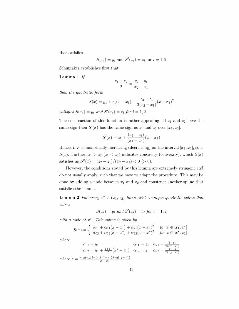
that satisfies

S(xi) = yi and S′(xi) = zi for i = 1, 2

Schumaker establishes first that

Lemma 1 Ifz1 + z2

2=

y2 − y1x2 − x1

then the quadratic form

S(x) = y1 + z1(x− x1) +z2 − z1

2(x2 − x1)(x− x1)

2

satisfies S(xi) = yi and S′(xi) = zi for i = 1, 2.

The construction of this function is rather appealing. If z1 and z2 have the

same sign then S ′(x) has the same sign as z1 and z2 over [x1;x2]:

S′(x) = z1 +(z2 − z1)

(x2 − x1)(x− x1)

Hence, if F is monotically increasing (decreasing) on the interval [x1;x2], so is

S(x). Further, z1 > z2 (z1 < z2) indicates concavity (convexity), which S(x)

satisfies as S ′′(x) = (z2 − z1)/(x2 − x1) < 0 (> 0).

However, the conditions stated by this lemma are extremely stringent and

do not usually apply, such that we have to adapt the procedure. This may be

done by adding a node between x1 and x2 and construct another spline that

satisfies the lemma.

Lemma 2 For every x? ∈ (x1, x2) there exist a unique quadratic spline that

solves

S(xi) = yi and S′(xi) = zi for i = 1, 2

with a node at x?. This spline is given by

S(x) =

α01 + α11(x− x1) + α21(x− x1)

2 for x ∈ [x1;x?]

α02 + α12(x− x?) + α22(x− x?)2 for x ∈ [x?;x2]

whereα01 = y1 α11 = z1 α21 =

z−z12(x?−x1)

α02 = y1 +z+z12 (x? − x1) α12 = z α22 =

z2−z2(x2−x?)

where z = 2(y2−y1)−(z1(x?−x1)+z2(x2−x?)x2−x1

42

If the later lemma fully characterized the quadratic spline, it gives no informa-

tion on x? which therefore remains to be selected. x? will be set such that the

spline matches the desired shape properties. First note that if z1 and z2 are

both positive (negative), then S(x) is monotone if and only if z1z > 0 (6 0)

which is actually equivalent to

2(y2 − y1) R (x? − x1)z1 + (x2 − x?)z2 if z1, z2 R 0

This essentially deals with the monotonicity problem, and we now have to

tackle the question of curvature. To do so, we compute the slope of the secant

line between x1 and x2

∆ =y2 − y1x2 − x1

Then, if (z2−∆)(z1−∆) > 0, this indicates the presence of an inflexion point

in the interval [x1;x2] such that the interpolant cannot be neither convex nor

concave. Conversely, if |z2 −∆| < |z1 −∆| and x? satisfies

x1 < x? 6 x ≡ x1 +2(x2 − x1)(z2 −∆)

(z2 − z1)

then S(x), as described in the latter lemma, is convex (concave) if z1 < z2

(z1 > z2). Further, if z1z2 > 0 it is also monotone.

If, on the contrary, |z2 −∆| > |z1 −∆| and x? satisfies

x ≡ x2 +2(x2 − x1)(z1 −∆)

(z2 − z1)6 x? < x2

then S(x), as described in the latter lemma, is convex (concave) if z1 < z2

(z1 > z2).

This therefore endow us with a range of values for x? that will insure that

shape properties will be preserved.

1. Check if lemma 1 is satisfied. If so set x? = x2 and set S(x) as in lemma

2. Then stop else go to 2.

2. Compute ∆ = y2 − y1/x2 − x1

43

3. if (z1 −∆)(z2 −∆) > 0 set x? = (x1 + x2)/2 and stop else goto 4.

4. if |z1 −∆| < |z2 −∆| set x? = (x1 + x)/2 and stop else goto 5.

5. if |z1 −∆| > |z2 −∆| set x? = (x2 + x)/2 and stop.

We have then in hand a value for x? for [x1;x2]. We then apply it to each

sub–interval to get x?i ∈ [xi;xi+1] and then solve the general interpolation

problem as explained in lemma 2.

Note here that everything assumes that with have Hermite data in hand —

i.e. xi, yi, zi : i = 0, . . . , n. However, the knowledge of the slope is usually

not the rule and we therefore have to adapt the algorithm to such situations.

3.7.2 Unknown slope: back to Lagrange interpolation

Assume now that we do not have any data for the slope of the function, that

is we are only endowed with Lagrange data xi, yi : i = 0, . . . , n. In such a

case, we just have to add the needed information — an estimate of the slope of

the function — and proceed exactly as in Hermite interpolation. Schumaker

proposes the following procedure to get zi; i = 1, . . . , n. Compute

Li =[(xi+1 − xi)

2 + (yi+1 − yi)2] 1

2

and

∆i =yi+1 − yixi+1 − xi

for i = 1, . . . , n− 1. Then zi, i = 1, . . . , n can be recovered as

zi =

Li−1∆i−1 + Li∆i

Li−1 + Liif ∆i−1∆i > 0

0 if ∆i−1∆i 6 0i = 2, . . . , n− 1

and

z1 = −3∆1 − z2

2and zn =

3∆n−1 − sn−12

Then, we just apply exactly the same procedure as described in the previous

section.

44

Up to now, all methods we have been studying are uni–dimensional whereas

most of the model we deal with in economics involve more than 1 variable.

We therefore need to extend the analysis to higher dimensional problems.

3.8 Multidimensional approximations

Computing a multidimensional approximation to a function may be quite cum-

bersome and even impossible in some cases. To understand the problem, let

us restate an example provided by Judd [1998]. Consider we have data points

P1, P2, P3, P4 = (1, 0), (−1, 0), (0, 1), (0,−1) in R2 and the corresponding

data zi = F (Pi), i = 1, . . . , 4. Assume now that we want to construct the ap-

proximation of function F using a linear combination of 1, x, y, xy defined

as

G(x, y) = a+ bx+ cy + dxy

such that G(xi, yi) = zi. Finding a, b, c, d amounts to solve the linear system

1 1 0 01 −1 0 01 0 1 01 0 −1 0

abcd

=

z1z2z3z4

which is not feasible as the matrix is not full rank.

This example reveals two potential problems:

1. Approximation in higher dimensional systems involves cross–product

and therefore poses the problem of the selection of polynomial basis

to be used for approximation,

2. More important is the selection of the grid of nodes used to evaluate the

function to compute the approximation.

We now investigate these issues, by first considering the simplest way to

attack the question — namely considering tensor product bases — and then

moving to a second way of dealing with this problem — considering complete

polynomials. In each case, we explain how Chebychev approximations can be

obtained.

45

3.8.1 Tensor product bases

The idea here is to use the tensor product of univariate functions to form a

basis of multivariate functions. In order to better understand this point, let

us consider that we want to approximate a function F : R2 −→ R using simple

univariate monomials up to order 2: X = 1, x, x2 and Y = 1, y, y2. Thetensor product basis is given by

1, x, y, xy, x2, y2, x2y, xy2, x2y2

i.e. all possible 2–terms products of elements belonging to X and Y .

We are now in position to define the n–fold tensor product basis for func-

tions of n variables x1, . . . , xi, . . . , xn.

Definition 10 Given a basis for n functions of the single variable xi: Pi =

pki (xi)κik=0 then the tensor product basis is given by

B =

κ1∏

k1=0

. . .

κn∏

kn=0

pk11 (x1) . . . p

knn (xn)

An important problem with this type of tensor product basis is their size.

For example, considering a m–dimensional space with polynomials of order

n, we already get (n + 1)m terms! This exponential growth in the number

of terms makes it particularly costly to use this type of basis, as soon as the

number of terms or the number of nodes is high. Nevertheless, it will often

be satisfactory or sufficient for low enough polynomials (in practice n=2!)

Therefore, one often rely on less computationally costly basis.

3.8.2 Complete polynomials

As aforementioned, tensor product bases grow exponentially as the dimension

of the problem increases, complete polynomials have the great advantage of

growing only polynomially as the dimension increases. From an intuitive point

of view, complete polynomials bases take products of order lower than a priori

given κ into account, ignoring higher terms of higher degrees.

46

Definition 11 For κ ∈ N given, the complete set of polynomials of total degree

κ in n variables is given by

Bc =

xk11 × . . .× xknn : k1, . . . , kn > 0,

n∑

i=1

ki 6 κ

To see this more clearly, let us consider the example developed in the previous

section (X = 1, x, x2 and Y = 1, y, y2) and let us assume that κ = 2. In

this case, we end up with a complete polynomials basis of the type

Bc =

1, x, y, x2, y2, xy

= B\xy2, x2y, x2y2

Note that we have actually already encountered this type of basis, as this is

typically what is done by Taylor’s theorem for many dimensions

F (x) ' F (x?) +n∑

i=1

∂F

∂xi(x?)(xi − x?i )

...

+1

k!

n∑

i1=1

. . .n∑

ik=1

∂F

∂xi1 . . . ∂xi1(x?)(xi1 − x?i1) . . . (xik − x?ik)

For instance, considering the Taylor expansion to the 2–dimensional function

F (x, y) around (x?, y?) we get

F (x, y) ' F (x?, y?) + Fx(x?, y?)(x− x?) + Fy(x

?, y?)(y − y?)

+1

2

(Fxx(x

?, y?)(x− x?)2 + 2Fxy(x?, y?)(x− x?)(y − y?)

+Fyy(x?, y?)(y − y?)2

)

which rewrites

F (x, y) = α0 + α1x+ α2y + α3x2 + α4y

2 + α5xy

such that the implicit polynomial basis is the complete polynomials basis of

order 2 with 2 variables.

47

The key difference between tensor product bases and complete polynomi-

als bases lies essentially in the rate at which the size of the basis increases. As

aforementioned, tensor product bases grow exponentially while complete poly-

nomials bases only grow polynomially. This reduces the computational cost of

approximation. But what do we loose using complete polynomials rather than

tensor product bases? From a theoretical point of view, Taylor’s theorem gives

us the answer: Nothing! Indeed, Taylor’s theorem indicates that the element

in Bc delivers a approximation in the neighborhood of x? that exhibits an

asymptotic degree of convergence equal to k. The n–fold tensor product, B,

can deliver only a kth degree of convergence as it does not contains all terms

of degree k + 1. In other words, complete polynomials and tensor product

bases deliver the same degree of asymptotic convergence and therefore com-

plete polynomials based approximation yields an as good level of accuracy as

tensor product based approximations.

Once we have chosen a basis, we can proceed to approximation. For ex-

ample, we may use Chebychev approximation in higher dimensional problems.

Judd [1998] reports the algorithm for this problem. As we will see, it takes ad-

vantage of a very nice feature of orthogonal polynomials: they inherit their or-

thogonality property even if we extend them to higher dimensions. Let us then

assume we want to compute the chebychev approximation of a 2–dimensional

function F (x, y) over the interval [ax; bx] × [ay; by] and let us assume — to

keep things simple for a while — that we use a tensor product basis. Then

the algorithm is as follows

1. Choose a polynomial order for x (nx) and y (ny)

2. Compute mx > nx + 1 and my > ny + 1 Chebychev interpolation nodes

on [−1; 1]zxk = cos

(2k − 1

2mxπ

), k = 1, . . . ,mx

and

zyk = cos

(2k − 1

2myπ

), k = 1, . . . ,my

48

3. Adjust the nodes to fit in both interval

xk = ax + (1 + zxk )

(bx − ax

2

), k = 1, . . . ,mx

and

yk = ay + (1 + zyk)

(by − ay

2

), k = 1, . . . ,my

4. Evaluate the function F at each node to form

Ω ≡ ωk` = F (xk, y`) : k = 1, . . . ,mx; ` = 1, . . . ,my

5. Compute the (nx+1)×(ny+1) Chebychev coefficients αij , i = 0, . . . , nx,

j = 0, . . . , ny as

αij =

mx∑

k=1

my∑

`=1

ωk`Txi (zxk )T

yj

(zy`)

(mx∑

k=1

T xi (zxk )

2

)(my∑

`=1

T yj

(zy`)2)

which may be simply obtained in this case as

α =T x(zx)′ΩT y(zy)

‖T x(zx)‖2 × ‖T y(zy)‖2

6. Compute the approximation as

G(x, y) =

nx∑

i=0

ny∑

j=0

αijTxi

(2x− axbx − ax

− 1

)T yj

(2y − ayby − ay

− 1

)

which may also be obtained as

G(x, y) = T x

(2x− axbx − ax

− 1

)αT y

(2y − ayby − ay

− 1

)′

As an illustration of the algorithm we compute the approximation of the CES

function

F (x, y) = [xρ + yρ]1ρ

49

on the [0.01; 2]×[0.01; 2] interval for ρ = 0.75. We used 5–th order polynomials

for both x and y and 20 nodes for both x and y, such that there are 400

possible interpolation nodes. Applying the algorithm we just described, we

get the matrix of coefficients reported in table 3.7. As can be seen from the

table, most of the coefficients are close to zero as soon as they involve the

cross–product of higher order terms, such that using a complete polynomial

basis would yield the same efficiency at a lower computational cost. Figure

3.10 reports the graph of the residuals for the approximation.

Table 3.7: Matrix of Chebychev coefficients (tensor product basis)

kx \ ky 0 1 2 3 4 5

0 2.4251 1.2744 -0.0582 0.0217 -0.0104 0.00571 1.2744 0.2030 -0.0366 0.0124 -0.0055 0.00292 -0.0582 -0.0366 0.0094 -0.0037 0.0018 -0.00093 0.0217 0.0124 -0.0037 0.0016 -0.0008 0.00054 -0.0104 -0.0055 0.0018 -0.0008 0.0004 -0.00035 0.0057 0.0029 -0.0009 0.0005 -0.0003 0.0002

Matlab Code: Chebychev Coefficients in R2 (Tensor Product Basis)

rho = 0.75;

mx = 20;

my = 20;

nx = 5;

ny = 5;

ax = 0.01;

bx = 2;

ay = 0.01;

by = 2;

%

% Step 1

%

rx = cos((2*[1:mx]’-1)*pi/(2*mx));

ry = cos((2*[1:my]’-1)*pi/(2*my));

%

% Step 2

%

x = (rx+1)*(bx-ax)/2+ax;

y = (ry+1)*(by-ay)/2+ay;

50

%

% Step 3

%

Y = zeros(mx,my);

for ix=1:mx;

for iy=1:my;

Y(ix,iy) = (x(ix)^rho+y(iy)^rho)^(1/rho);

end

end

%

% Step 4

%

Xx = [ones(mx,1) rx];

for i=3:nx+1;

Xx= [Xx 2*rx.*Xx(:,i-1)-Xx(:,i-2)];

end Xy = [ones(my,1) ry];

for i=3:ny+1;

Xy= [Xy 2*ry.*Xy(:,i-1)-Xy(:,i-2)];

end

T2x = diag(Xx’*Xx);

T2y = diag(Xy’*Xy);

a = (Xx’*Y*Xy)./(T2x*T2y’);

Figure 3.10: Residuals: Tensor product basis

00.5

11.5

2

0

0.5

1

1.5

2

−0.015

−0.01

−0.005

0

0.005

0.01

xy

51

If we now want to perform the same approximation using a complete poly-

nomials basis, we just have to modify the algorithm to take into account the

fact that when iterating on i and j we want to impose i + j 6 κ. Let us

compute is for κ = 5. This implies that the basis will consists of

1, T x1 (.), T

y1 (.), T

x2 (.), T

y2 (.), T

x3 (.), T

y3 (.), T

x4 (.), T

y4 (.), T

x5 (.), T

y5 (.),

T x1 (.)T

y1 (.), T

x1 (.)T

y2 (.), T

x1 (.)T

y3 (.), T

x1 (.)T

y4 (.),

T x2 (.)T

y1 (.), T

x2 (.)T

y2 (.), T

x2 (.)T

y3 (.),

T x3 (.)T

y1 (.), T

x3 (.)T

y2 (.),

T x4 (.)T

y1 (.)

Table 3.8: Matrix of Chebychev coefficients (Complete polynomials basis)

kx \ ky 0 1 2 3 4 5

0 2.4251 1.2744 -0.0582 0.0217 -0.0104 0.00571 1.2744 0.2030 -0.0366 0.0124 -0.0055 –2 -0.0582 -0.0366 0.0094 -0.0037 – –3 0.0217 0.0124 -0.0037 – – –4 -0.0104 -0.0055 – – – –5 0.0057 – – – – –

A first thing to note is that the coefficients that remain are the same as

the one we got in the tensor product basis. This should not be any surprise

as what we just find is just the expression of the Chebychev economization we

already encountered in the uni–dimensional case and which is just the direct

consequence of the orthogonality condition of chebychev polynomials. Figure

3.11 report the residuals from the approximation using the complete basis. As

can be seen from the figure, this “constrained” approximation yields quantita-

tively similar results compared to the tensor product basis, therefore achieving

almost the same accuracy while being less costly from a computational point

of view. In the matlab code section, we just report the lines in step 4 that

are affected by the adoption of the complete polynomials basis.

52

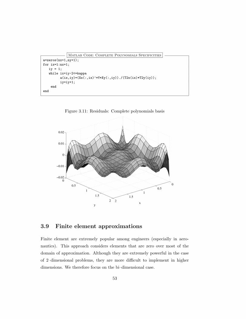
Matlab Code: Complete Polynomials Specificities

a=zeros(nx+1,ny+1);

for ix=1:nx+1;

iy = 1;

while ix+iy-2<=kappa

a(ix,iy)=(Xx(:,ix)’*Y*Xy(:,iy))./(T2x(ix)*T2y(iy));

iy=iy+1;

end

end

Figure 3.11: Residuals: Complete polynomials basis

00.5

11.5

2

0

0.5

1

1.5

2

−0.02

−0.01

0

0.01

0.02

xy

3.9 Finite element approximations

Finite element are extremely popular among engineers (especially in aero-

nautics). This approach considers elements that are zero over most of the

domain of approximation. Although they are extremely powerful in the case

of 2–dimensional problems, they are more difficult to implement in higher

dimensions. We therefore focus on the bi–dimensional case.

53

3.9.1 Bilinear approximations

A bilinear interpolation proposes to interpolate data linearly in both coordi-

nate directions. Assume that we have the values of a function F (x, y) at the

four pointsP1 = (−1,−1) P2 = (−1, 1)P3 = (1,−1) P4 = (1, 1)

A cardinal interpolation basis on [−1; 1] × [−1; 1] is provided by the set of

functions

b1(x, y) =14(1− x)(1− y) b2(x, y) =

14(1− x)(1 + y)

b3(x, y) =14(1 + x)(1− y) b4(x, y) =

14(1 + x)(1 + y)

All functions bi are zero on all Pj , i 6= j, but on the point to which is associated

the same index (i = j). Therefore, an approximation of F (x, y) on [−1; 1] ×[−1; 1] is given by

F (x, y) ' F (−1,−1)b1(x, y)+F (−1, 1)b2(x, y)+F (1,−1)b3(x, y)+F (1, 1)b4(x, y)

If we have data on [ax; bx]× [ay; by], we use the linear transformation we have

already encountered a great number of times(2x− axbx − ax

− 1, 2y − ayby − ay

− 1

)

Then, if we have Lagrange data of the type xi, yi, zi : i = 1, . . . , n, we

proceed as follows

1. Construct a grid of nodes for x and y;

2. Construct the interpolant over each square applying the previous scheme;

3. Piece all interpolant together.

Note that an important issue of piecewise interpolation is related to the con-

tinuity of the approximation: individual pieces must meet continuously at

common edges. In bilinear interpolation, this is insured by the fact that two

interpolants overlap only at the edges of rectangles on which the approxi-

mation is a linear interpolant of 2 common end points. This would not be

54

insured if we were to construct bi–quadratic or bi–cubic interpolations for ex-

ample. Note that this type of interpolation scheme is typically what is done

when a computer draw a 3d graph of a function. In figure 3.12, we plot

the residuals of the bilinear approximation of the CES function we approxi-

mated in the previous section, with 5 uniform intervals (6 nodes such that x =

0.010, 0.408, 0.806, 1.204, 1.602, 2.000 and y = 0.010, 0.408, 0.806, 1.204, 1.602, 2.000).Like in the spline approximation procedure, the most difficult step once we

have obtained an approximation is to determine the square the point for which

we want an approximation belongs to. We therefore face exactly the same type

of problems.

Figure 3.12: Residuals of the bilinear approximation

0

0.5

1

1.5

2 00.5

11.5

2

−1

−0.5

0

0.5

1

yx

3.9.2 Simplicial 2D linear interpolation

This method essentially amounts to consider triangles rather than rectangles

as an approximation basis. The idea is then to build triangles in the x − −yplane. To do so, and assuming that the lagrange data have already been

55

transformed using the linear map described earlier, we set 3 points

P1 = (0, 0), P2 = (0, 1), P3 = (1, 0)

to which we associate 3 functions

b1(x, y) = 1− x− y, b2(x, y) = y, b3(x, y) = x

which are such that all functions bi are zero on all Pj , i 6= j, but on the point

to which is associated the same index (i = j). b1 b2 and b3 are the cardinal

functions on P1, P2, P3. Let us now add the point P4 = (1, 1), then we have

the following cardinal functions for P2, P3, P4:

b4(x, y) = 1− x, b5(x, y) = 1− y, b6(x, y) = x+ y − 1

Therefore, on the square P1, P2, P3, P4 the interpolant for F is given by

G(x, y) =

F (0, 0)(1− x− y) + F (0, 1)y + F (1, 0)x if x+ y 6 1

F (0, 1)(1− x) + F (1, 0)(1− y) + F (1, 1)(x+ y − 1) if x+ y > 1

It should be clear to you that if these methods are pretty easy to implement

in dimension 3, it becomes quite cumber some in higher dimensions, and noth

that much is proposed in the literature, are most of these methods were de-

signed by engineers and physicists that essentially have to deal with 2, 3 at

most 4 dimensional problems. We will see that this will be a limitation in a

number of economic applications.

56

Bibliography

Hornik, K., M. Stinchcombe, and H. White, Multi–Layer Feedforward Net-

works are Universal Approximators, Neural Networks, 1989, 2, 359–366.

Judd, K.L., Numerical methods in economics, Cambridge, Massachussets:

MIT Press, 1998.

Schumaker, L.L., On Shape–preseving Quadratic Spline Interpolation, SIAM

Journal of Numerical Analysis, 1983, 20, 854–864.

57

Index

Analytic function, 4

Chebychev approximation, 24

Complete polynomials, 47

complete polynomials, 46

Economization principle, 28

Hidden–layer feedforward, 14

Least square orthogonal polynomial

approximation, 19

Linearization, 6

Local approximations, 2

Log–linearization, 7

Multidimensional approximation, 45

Neural networks, 11

Ordinary least square, 8

Orthogonal polynomials, 18

Radius of convergence, 3

Single–layer, 14

Splines, 32

Taylor series expansion, 2

Tensor product bases, 46

Vandermonde matrix, 23

58

Contents

3 Approximation Methods 1

3.1 Local approximations . . . . . . . . . . . . . . . . . . . . . . . 2

3.1.1 Taylor series expansion . . . . . . . . . . . . . . . . . . 2

3.2 Regressions as approximation . . . . . . . . . . . . . . . . . . . 8

3.2.1 Orthogonal polynomials . . . . . . . . . . . . . . . . . . 18

3.3 Least square orthogonal polynomial approximation . . . . . . . 19

3.4 Interpolation methods . . . . . . . . . . . . . . . . . . . . . . . 22

3.4.1 Linear interpolation . . . . . . . . . . . . . . . . . . . . 22

3.4.2 Lagrange interpolation . . . . . . . . . . . . . . . . . . . 23

3.5 Chebychev approximation . . . . . . . . . . . . . . . . . . . . . 24

3.6 Piecewise interpolation . . . . . . . . . . . . . . . . . . . . . . . 32

3.7 Shape preserving approximations . . . . . . . . . . . . . . . . . 41

3.7.1 Hermite interpolation . . . . . . . . . . . . . . . . . . . 41

3.7.2 Unknown slope: back to Lagrange interpolation . . . . . 44

3.8 Multidimensional approximations . . . . . . . . . . . . . . . . . 45

3.8.1 Tensor product bases . . . . . . . . . . . . . . . . . . . . 46

3.8.2 Complete polynomials . . . . . . . . . . . . . . . . . . . 47

3.9 Finite element approximations . . . . . . . . . . . . . . . . . . 53

3.9.1 Bilinear approximations . . . . . . . . . . . . . . . . . . 53

3.9.2 Simplicial 2D linear interpolation . . . . . . . . . . . . . 55

59

60

List of Figures

3.1 Selection of points . . . . . . . . . . . . . . . . . . . . . . . . . 10

3.2 Least–square approximation of consumption . . . . . . . . . . . 13

3.3 Neural Networks . . . . . . . . . . . . . . . . . . . . . . . . . . 14

3.4 Neural Network Approximation . . . . . . . . . . . . . . . . . . 17

3.5 Chebychev polynomials . . . . . . . . . . . . . . . . . . . . . . 25

3.6 Smooth function: F (x) = x0.1 . . . . . . . . . . . . . . . . . . . 29

3.7 Non–smooth function: F (x) = min(max(−1.5, (x− 1/2)3), 2) . 31

3.8 Cubic spline approximation . . . . . . . . . . . . . . . . . . . . 38

3.9 Approximation errors . . . . . . . . . . . . . . . . . . . . . . . 39

3.10 Residuals: Tensor product basis . . . . . . . . . . . . . . . . . . 52

3.11 Residuals: Complete polynomials basis . . . . . . . . . . . . . . 54

3.12 Residuals of the bilinear approximation . . . . . . . . . . . . . 56

61

62

List of Tables

3.1 Taylor series expansion for log(1− x) . . . . . . . . . . . . . . . 5

3.2 Neural Network approximation . . . . . . . . . . . . . . . . . . 17

3.3 Orthogonal polynomials (definitions) . . . . . . . . . . . . . . . 19

3.4 Orthogonal polynomials (recursive representation) . . . . . . . 20

3.5 Chebychev Coefficients: Smooth function . . . . . . . . . . . . 29

3.6 Chebychev Coefficients: Non–smooth function . . . . . . . . . . 31

3.7 Matrix of Chebychev coefficients (tensor product basis) . . . . 50

3.8 Matrix of Chebychev coefficients (Complete polynomials basis) 52

63