Approximating ATSP by Relaxing Connectivity

Ola SvenssonEPFL

ola.svensson@epfl.ch

August 14, 2015

Abstract

The standard LP relaxation of the asymmetric traveling salesman problem hasbeen conjectured to have a constant integrality gap in the metric case. We prove thisconjecture when restricted to shortest path metrics of node-weighted digraphs. Ourarguments are constructive and give a constant factor approximation algorithmfor these metrics. We remark that the considered case is more general than thedirected analog of the special case of the symmetric traveling salesman problemfor which there were recent improvements on Christofides’ algorithm.

The main idea of our approach is to first consider an easier problem obtained bysignificantly relaxing the general connectivity requirements into local connectivityconditions. For this relaxed problem, it is quite easy to give an algorithm witha guarantee of 3 on node-weighted shortest path metrics. More surprisingly, wethen show that any algorithm (irrespective of the metric) for the relaxed problemcan be turned into an algorithm for the asymmetric traveling salesman problem byonly losing a small constant factor in the performance guarantee. This leaves openthe intriguing task of designing a “good” algorithm for the relaxed problem ongeneral metrics.

Keywords: approximation algorithms, asymmetric traveling salesman problem, combinatorialoptimization, linear programming

arX

iv:1

502.

0205

1v2

[cs

.DS]

13

Aug

201

5

1 Introduction

The traveling salesman problem is one of the most fundamental combinatorial optimiza-tion problems. Given a set V of n cities and a distance/weight function w : V ×V → R+,it is the problem of finding a tour of minimum total weight that visits each city exactlyonce. There are two variants of this general definition: the symmetric traveling salesmanproblem (STSP) and the asymmetric traveling salesman problem (ATSP). In the symmet-ric version we assume w(u, v) = w(v,u) for each pair u, v ∈ V of cities; whereas we makeno such assumption in the more general asymmetric traveling salesman problem.

In both versions, it is common to assume the triangle inequality and we shall do soin the rest of this paper. Recall that the triangle inequality says that for any triple i, j, kof cities, we have w(i, j) + w( j, k) > w(i, k). In other words, it is not more expensive totake the direct path compared to a path that makes a detour. Another equivalent viewof the triangle inequality is that, instead of insisting that each city is visited exactly once,we should find a tour that visits each city at least once. These assumptions are arguablynatural in many, if not most, settings. They are also necessary in the following sense:any reasonable approximation algorithm (with approximation guarantee O(exp(n))) forthe traveling salesman problem without the triangle inequality would imply P = NPbecause it would solve the problem of deciding Hamiltonicity.

Understanding the approximability of the symmetric and the asymmetric travelingsalesman problem (where we have the triangle inequality) turns out to be a muchmore interesting and notorious problem. On the one hand, the strongest knowninapproximability results, by Karpinski, Lampis, and Schmied [14], say that it isNP-hard to approximate STSP within a factor of 123/122 and that it is NP-hard toapproximate ATSP within a factor of 75/74. On the other hand, the current bestapproximation algorithms are far from these guarantees, especially in the case of ATSP.

For the symmetric traveling salesman problem, Christofides’ beautiful algorithmfrom 1976 sill achieves the best known approximation guarantee of 1.5 [7]. However,a recent series of papers [11, 16, 17, 19], broke this barrier for the interesting specialcase of shortest path metrics of unweighted undirected graphs1. Specifically, OveisGharan, Saberi, and Singh [11] first gave an approximation guarantee of 1.5− ε; Mömkeand Svensson [16] proposed a different approach yielding a 1.461-approximationguarantee; Mucha [17] gave a tighter analysis of this algorithm; and Sebö and Vygen [19]significantly developed the approach to give the current best approximation guaranteeof 1.4.

The interest in shortest path metrics has several motivations. It is a natural specialcase that seems to capture the difficulty of the problem: it remains APX-hard and theworst known integrality gap for the Held-Karp relaxation is of this type. Moreover,it has an attractive graph theoretic formulation: given an unweighted graph, find ashortest tour that visits each vertex at least once. This is the (unweighted) “graph”analog of STSP. Indeed, if allow the graph to be edge-weighted, this formulationis equivalent to STSP on general metrics. Let us also mention that the polynomialtime approximation scheme for the symmetric traveling salesman problem on planar

1The shortest path metric of a graph G = (V,E) is defined as follows: the weight w(u, v) between citiesu, v ∈ V equals the shortest path between u and v in G. If the graph is node-weighted f : V → R+, theweight/length of an edge {u, v} ∈ E is f (u) + f (v).

2

graphs was first obtained for the special case of unweighted graphs [12], i.e., whenrestricted to shortest path metrics of unweighted graphs, and then generalized to thecase of edge-weights [3]. For STSP, it remains a major open problem whether the ideasin [11, 16, 17, 19] can be applied to general metrics. We further discuss this in Section 6.

The gap in our understanding is much larger for the asymmetric traveling salesmanproblem for which it remains a notorious open problem to design an algorithm with anyconstant approximation guarantee. This is a particularly intriguing as the standard linearprogramming relaxation, often referred to as the Held-Karp relaxation, is only knownto have an integrality gap of at least 2 [6]. There are in general two available approachesfor designing approximation algorithms for ATSP in the literature. The first approachis due to Frieze, Galbiati, and Maffiolo [9] who gave a log2(n)-approximation algorithmfor ATSP already in 1982. Their basic idea is simple and elegant: a minimum weightcycle cover has weight at most that of an optimal tour and it will decrease the numberof connected components by a factor of at least 2. Hence, if we repeat the selection of aminimum weight cycle cover log2(n) times, we get a connected Eulerian graph which(by shortcutting) is a log2(n)-approximate tour. Although the above analysis is tightonly in the case when almost all cycles in the cycle covers have length 2, it is highlynon-trivial to refine the method to decrease the number of iterations. It was first in 2003that Bläser [5] managed to give an approximation guarantee of 0.999 log2(n). This wasimproved shortly thereafter by Kaplan, Lewenstein, Shafrir and Sviridenko [13] whofurther developed this approach to obtain a 4/3 log3(n) ≈ 0.84 log2(n)-approximationalgorithm; and later by Feige and Singh [8] who obtained an approximation guaranteeof 2/3 log2(n).

A second approach was more recently proposed in an influential and beautifulpaper by Asadpour, Goemans, Madry, Oveis Gharan, and Saberi [4] who gave anO(log n/ log log n)-approximation algorithm for ATSP. Their approach is based onfinding a so-called α-thin spanning tree which is a (unweighted) graph theoreticproblem. Here, the parameter α is proportional to the approximation guarantee soα = O(log n/ log log n) in [4]. Following their publication, Oveis Gharan and Saberi [10]gave an efficient algorithm for finding O(1)-thin spanning trees for planar and boundedgenus graphs yielding a constant factor approximation algorithm for ATSP on thesegraph classes. Also, in a very recent major progress, Anari and Oveis Gharan [1]showed the existence of O(polylog log n)-thin spanning trees for general instances.This implies a O(polylog log n) upper bound on the integrality gap of the Held-Karprelaxation. Hence, it gives an efficient so-called estimation algorithm for estimatingthe optimal value of a tour within a factor O(polylog log n) but, as their arguments arenon-constructive, no approximation algorithm for finding a tour of matching guarantee.The result in [1] is based on developing and extending several advanced techniques.Notably, they rely on their extension [2] of the recent proof of the Kadison-Singerconjecture which was a major breakthrough by Marcus, Spielman, and Srivastava [15].

To summarize, the current best approximation algorithm has a guarantee ofO(log n/ log log n) [4] and the best upper bound on the integrality gap of the Held-Karprelaxation is O(polylog log n) [1]. These two bounds are far away from the knowninapproximability results [14] and from the lower bound of 2 on the integrality gap ofthe Held-Karp relaxation [6]. Moreover, there were no better approximation algorithms

3

known in the case of shortest path metrics of unweighted digraphs for which there wasrecent progress in the undirected setting. In particular, it is not clear how to use the twoavailable approaches mentioned above to get an improved approximation guarantee inthis case: in the cycle cover approach, the main difficulty is to bound the number ofiterations and, in the thin spanning tree approach, ATSP is reduced to an unweightedgraph theoretic problem.

1.1 Our Results and Overview of Approach

We propose a new approach for approximating the asymmetric traveling salesmanproblem based on relaxing the global connectivity constraints into local connectivityconditions. We also use this approach to obtain the following result where we refer toATSP on shortest path metrics of node-weighted digraphs as Node-Weighted ATSP.

Theorem 1.1. There is a constant approximation algorithm for Node-Weighted ATSP. Specifi-cally, for Node-Weighted ATSP, the integrality gap of the Held-Karp relaxation is at most 15and, for any ε > 0, there is a polynomial time algorithm that finds a tour of weight at most(27 + ε) OPTHK where OPTHK denotes the optimal value of the Held-Karp relaxation.

As further discussed in Section 6, the constants in the theorem can be slightlyimproved by specializing our general approach to the node-weighted case. However,it remains an interesting open problem to give a tight bound on the integrality gap.

Let us continue with a brief overview of our approach that is not restricted to thenode-weighted version. It is illustrative to consider the following “naive” algorithmthat actually was the starting point of this work:

1. Select a random cycle cover C using the Held-Karp relaxation.

It is well known that one can sample such a cycle cover C of expected weightequal to the optimal value OPTHK of the Held-Karp relaxation.

2. While there exist more than one component, add the lightest cycle (i.e., the cycleof smallest weight) that decreases the number of components.

It is clear that the above algorithm always returns a solution to ATSP: we start witha Eulerian graph2 and the graph stays Eulerian during the execution of the while-loop which does not terminate until the graph is connected. This gives a tour thatvisits each vertex at least once and hence a solution to ATSP (using that we havethe triangle-inequality). However, what is the weight of the obtained tour? First, asremarked above, we have that the expected weight of the cycle cover is OPTHK. So ifC contains k = |C| cycles, we would expect that a cycle in C has weight OPTHK /k (atleast on average). Moreover, the number of cycles added in Step 2 is at most k − 1 sinceeach cycle decreases the number of components by at least one. Thus, if each cycle inStep 2 has weight at most the average weight OPTHK /k of a cycle in C, we obtain a2-approximate tour of weight at most OPTHK + k−1

k OPTHK 6 2 OPTHK.Unfortunately, it seems hard to find a cycle cover C so that we can always connect it

with light cycles. Instead, what we can do, is to first select a cycle cover C then add light

2Recall that a directed graph is Eulerian if the in-degree equals the out-degree of each vertex.

4

cycles that decreases the number of components as long as possible. When there are nomore light cycles to add, the vertices/cities are partitioned into V1, . . . ,Vk connectedcomponents. In order to make progress from this point, we would like to find a “light”Eulerian set F of edges that crosses the cuts {(Vi, Vi) | i = 1, 2, . . . , k}. We could thenhope to add F to our solution and continue from there. It turns out that it is veryimportant what “light” means in this context. For our arguments to work, we need thatF is selected so that the weight of the edges in each component has weight at most αtimes what the linear programming solution “pays” for the vertices in that component.This is the intuition behind the definitions in Section 3 of Local-Connectivity ATSP andα-light algorithms for that problem. We also need to be very careful in which way weadd edges from light cycles and how to use the α-light algorithm for Local-ConnectivityATSP. In Section 5, our algorithm will iteratively solve the Local-Connectivity ATSPand, in each iteration, it will add a carefully chosen subset of the found edges togetherwith light cycles.

We remark that in Local-Connectivity ATSP we have relaxed the global connectivityproperties of ATSP into local connectivity conditions that only say that we need to finda Eulerian set of edges that crosses at most n = |V| cuts defined by a partitioning of thevertices. In spite of that, we are able to leverage the intuition above to obtain our maintechnical result:

Theorem (Simplified statement of Theorem 5.1). The integrality gap of the Held-Karprelaxation is at most 5α if there exists an α-light algorithmA for Local-Connectivity ATSP.Moreover, for any ε > 0, we can find a (9 + ε)α-approximate tour in time polynomial in n, 1/ε,and in the running time ofA.

The proof of the above theorem (Section 5) is based on generalizing and, as alluded toabove, deviating from the above intuition in several ways. First, we start with a carefullychosen “Eulerian partition” which generalizes the role of the cycle cover C in Step 1above. Second, both the iterative use of the α-light algorithm for Local-ConnectivityATSP and the way we add light cycles are done in a careful and dependent manner so asto be able to bound the total weight of the returned solution. Theorem 1.1 follows fromTheorem 5.1 together with a 3-light algorithm for Node-Weighted Local-ConnectivityATSP. The 3-light algorithm, described in Section 4, is a rather simple application ofclassic theory of flows and circulations. We also remark that it is the only part of thepaper that relies on having shortest path metrics of node-weighted digraphs.

Our work raises several natural questions. Perhaps the most immediate andintriguing question is whether there is a O(1)-light algorithm for Local-ConnectivityATSP on general metrics. We further elaborate on this and other related questions inSection 6.

2 Preliminaries

2.1 Basic Notation

Consider a directed graph G = (V,E). For a subset S ⊆ V, we let δ+(S) = {(u, v) ∈ E |u ∈ S, v < S} be the outgoing edges and we let δ−(S) = {(u, v) ∈ E | u < S, v ∈ S} be the

5

incoming edges of the cut defined by S. When considering a subset E′ ⊆ E of the edges,we denote the restrictions to that subset by δ+

E′(S) = δ+(S)∩E′ and by δ−E′(S) = δ−(S)∩E′.We also let C(E′) = {G1 = (V1,E1), G2 = (V2, E2), . . . , Gk = (Vk, Ek)} denote the set ofsubgraphs corresponding to the k connected components of the graph (V,E′); the vertexset V will always be clear from the context. Here connected means that the subgraphsare connected if we undirect the edges.

When considering a function f : U → R, we let f (X) =∑

x∈X f (x) for X ⊆ U. Forexample, if G is edge weighted, i.e., there exists a function w : E→ R, then w(E′) denotesthe total weight of the edges in E′ ⊆ E. Similarly, if G is node-weighted, then thereexists a function f : V → R and f (S) denotes the total weight of the vertices in S ⊆ V.When talking about graphs, we shall slightly abuse notation and sometimes write w(G)instead of w(E) and f (G) instead of f (V) when it is clear from the context that w and fare functions on the edges and vertices. Finally, our subsets of edges are multisets, i.e., maycontain the same edge several times. The set operators ∪,∩, \ are defined in the naturalway. For example, {e1, e1, e2} ∪ {e1, e2} = {e1, e1, e1, e2, e2}, {e1, e1, e2} ∩ {e1, e2} = {e1, e2}, and{e1, e1, e2} \ {e1, e2} = {e1}. Other sets, such as subsets of vertices, will always be simplesets without any multiplicities.

2.2 The (Node-Weighted) Asymmetric Traveling Salesman Problem

It will be convenient to define ATSP using the Eulerian point of view, i.e., we wish tofind a tour that visits each vertex at least once. As already mentioned in the introduction,this definition is equivalent to that of visiting each city exactly once (in the metriccompletion) since we assume the triangle inequality.

ATSP

Given: An edge-weighted (strongly connected) digraph G = (V,E,w : E→ R+).

Find: A connected Eulerian digraph G′ = (V,E′) where E′ is a multisubset of E thatminimizes w(E′).

Similar to the recent progress on STSP, it is natural to consider special cases that areeasier to argue about but at the same time capture the combinatorial structure of theproblem. In particular, we shall consider the Node-Weighted ATSP, where we assumethat there exists a weight function f : V → R+ on the vertices so that w(u, v) = f (u).(Another equivalent definition, which also applies to undirected graphs, is to let theweight of an edge (u, v) be f (u) + f (v). This is equivalent to the definition above, ifscaled down by a factor of 2, since the solutions are Eulerian.)

Note that this generalizes ATSP on shortest path metrics of unweighted digraphs:that is the problem where f is the constant function. As a curiosity, we also note that therecent progress on STSP when restricted to shortest path metrics of unweighted graphsis not known to generalize to the node-weighted case. We raise this as an interestingopen problem in Section 6.

6

2.3 Held-Karp Relaxation

The Held-Karp relaxation has a variable xe > 0 for every edge in the given edge-weighted graph G = (V,E,w). The intended solution is that xe should equal the numberof times e is used in the solution. The relaxation LP(G) is now defined as follows:

minimize∑e∈E

xew(e)

subject to x(δ+(v)) = x(δ−(v)) v ∈ V,x(δ+(S)) > 1 ∅ , S ⊂ V,

x > 0.

The first set of constraints says that the in-degree should equal the out-degree for eachvertex, i.e., the solution should be Eulerian. The second set of constraints enforces thatthe solution is connected and they are sometimes referred to as subtour eliminationconstraints. For Node-Weighted ATSP, we can write the objective function of the linearprogram as

∑v∈V f (v) · x(δ+(v)), where f : V → R+ is the weights on the vertices that

defines the node-weighted metric.Finally, we remark that although the Held-Karp relaxation has exponentially many

constraints, it is well known that we can solve it in polynomial time either by using theellipsoid method with a separation oracle or by formulating an equivalent compact(polynomial size) linear program.

3 ATSP with Local Connectivity

In this section we define a seemingly easier problem than ATSP by relaxing theconnectivity requirements. Consider an optimal solution x∗ to LP(G). Its value, whichis a lower bound on OPT, can be decomposed into a “lower bound” for each vertex v:∑

e∈E

x∗ew(e) =∑v∈V

∑e∈δ+(v)

x∗ew(e).

︸ ︷︷ ︸lower bound for v

With this intuition, we let lb : V → R be the lower bound function defined bylbx∗,G(v) =

∑e∈δ+(v) x∗ew(e). We simplify notation and write lb instead of lbx∗,G as G will

always be clear from the context and therefore also x∗ (if the optimal solution to LP(G)is not unique then make an arbitrary but consistent choice). Note that lb(V) equals thevalue of the optimal solution to the Held-Karp relaxation.

Perhaps the main difficulty of ATSP is to satisfy the connectivity requirement, i.e.,to select a Eulerian subset F of edges that connects the whole graph. We shall now relaxthis condition to obtain what we call Local-Connectivity ATSP:

7

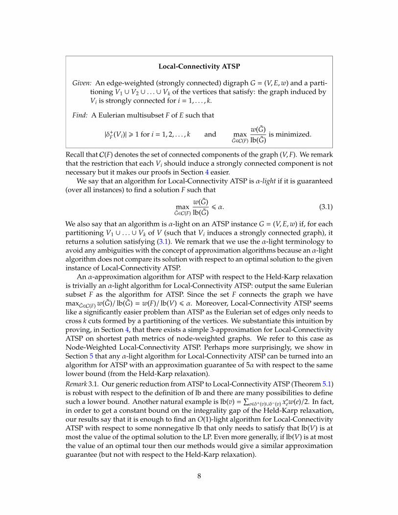
Local-Connectivity ATSP

Given: An edge-weighted (strongly connected) digraph G = (V,E,w) and a parti-tioning V1 ∪ V2 ∪ . . . ∪ Vk of the vertices that satisfy: the graph induced byVi is strongly connected for i = 1, . . . , k.

Find: A Eulerian multisubset F of E such that

|δ+F (Vi)| > 1 for i = 1, 2, . . . , k and max

G∈C(F)

w(G)lb(G)

is minimized.

Recall that C(F) denotes the set of connected components of the graph (V,F). We remarkthat the restriction that each Vi should induce a strongly connected component is notnecessary but it makes our proofs in Section 4 easier.

We say that an algorithm for Local-Connectivity ATSP is α-light if it is guaranteed(over all instances) to find a solution F such that

maxG∈C(F)

w(G)lb(G)

6 α. (3.1)

We also say that an algorithm is α-light on an ATSP instance G = (V,E,w) if, for eachpartitioning V1 ∪ . . . ∪ Vk of V (such that Vi induces a strongly connected graph), itreturns a solution satisfying (3.1). We remark that we use the α-light terminology toavoid any ambiguities with the concept of approximation algorithms because an α-lightalgorithm does not compare its solution with respect to an optimal solution to the giveninstance of Local-Connectivity ATSP.

An α-approximation algorithm for ATSP with respect to the Held-Karp relaxationis trivially an α-light algorithm for Local-Connectivity ATSP: output the same Euleriansubset F as the algorithm for ATSP. Since the set F connects the graph we havemaxG∈C(F) w(G)/ lb(G) = w(F)/ lb(V) 6 α. Moreover, Local-Connectivity ATSP seemslike a significantly easier problem than ATSP as the Eulerian set of edges only needs tocross k cuts formed by a partitioning of the vertices. We substantiate this intuition byproving, in Section 4, that there exists a simple 3-approximation for Local-ConnectivityATSP on shortest path metrics of node-weighted graphs. We refer to this case asNode-Weighted Local-Connectivity ATSP. Perhaps more surprisingly, we show inSection 5 that any α-light algorithm for Local-Connectivity ATSP can be turned into analgorithm for ATSP with an approximation guarantee of 5α with respect to the samelower bound (from the Held-Karp relaxation).Remark 3.1. Our generic reduction from ATSP to Local-Connectivity ATSP (Theorem 5.1)is robust with respect to the definition of lb and there are many possibilities to definesuch a lower bound. Another natural example is lb(v) =

∑e∈δ+(v)∪δ−(v) x∗ew(e)/2. In fact,

in order to get a constant bound on the integrality gap of the Held-Karp relaxation,our results say that it is enough to find an O(1)-light algorithm for Local-ConnectivityATSP with respect to some nonnegative lb that only needs to satisfy that lb(V) is atmost the value of the optimal solution to the LP. Even more generally, if lb(V) is at mostthe value of an optimal tour then our methods would give a similar approximationguarantee (but not with respect to the Held-Karp relaxation).

8

V1

A1

V2

A2

Figure 1: A depiction of the construction of the auxiliary graph G′ (in the proof ofTheorem 4.1): edges are subdivided, an auxiliary vertex Ai is added for each partitionVi, and Ai is “connected” to subdivisions of the edges in δ+(Vi) and δ−(Vi).

4 Approximating Local-Connectivity ATSP

We give a simple 3-light algorithm for Node-Weighted Local-Connectivity ATSP.The proof is based on finding an integral circulation that sends flow across the cuts{(Vi, Vi) : i = 1, 2, . . . , k} and, in addition, satisfies that the outgoing flow of each vertexv ∈ V is at most dx∗(δ+(v))e + 1 which in turn, by the assumptions on the metric, impliesa 3-light algorithm.

Theorem 4.1. There exists a polynomial time 3-light algorithm for Node-Weighted Local-Connectivity ATSP.

Proof. Let G = (V,E,w) and V1 ∪ V2 ∪ . . . ∪ Vk be an instance of Local-ConnectivityATSP where w : E→ R+ is a node-weighted metric defined by f : V → R+. Let also x∗

be an optimal solution to LP(G). We prove the theorem by giving a polynomial timealgorithm that finds a Eulerian multisubset F of E satisfying

|δ+F (Vi)| > 1 for i = 1, . . . , k and |δ+

F (v)| 6 dx∗(δ+(v))e + 1 for v ∈ V. (4.1)

To see that this is sufficient, note that the Eulerian set F forms a solution to the Local-Connectivity ATSP instance because |δ+

F (Vi)| > 1 for i = 1, . . . , k; and it is 3-light since,for each G = (V, E) ∈ C(F), we have (using that it is a node-weighted metric)

w(G)lb(G)

=

∑v∈V |δ

+E

(v)| f (v)∑v∈V x∗(δ+(v)) f (v)

6

∑v∈V(dx∗(δ+(v))e + 1) f (v)∑

v∈V x∗(δ+(v)) f (v)6 3.

The last inequality follows from x∗(δ+(v)) > 1 and therefore dx∗(δ+(v))e + 1 6 3x∗(δ+(v)).We proceed by describing a polynomial time algorithm for finding a Eulerian set F

satisfying (4.1). We shall do so by finding a circulation in an auxiliary graph G′ obtainedfrom G as follows (see also Figure 1):

1. Replace each edge e = (u, v) in G by adding vertices Oe, Ie and edges(u,Oe), (Oe, Ie), (Ie, v);

2. For each partition Vi, i = 1, . . . , k, add an auxiliary vertex Ai and edges (Ai,Oe) forevery e ∈ δ+(Vi) and (Ie,Ai) for every e ∈ δ−(Vi).

9

Recall that a circulation in G′ is a vector y with a nonnegative value for each edgesatisfying flow conservation: y(δ+(v)) = y(δ−(v)) for every vertex v. The followingclaim follows from the construction of G′ together with basic properties of flows andcirculations.Claim 4.2. We can in polynomial time find an integral circulation y in G′ satisfying:

y(δ+(Ai)) = 1 for i = 1, . . . , k and y(δ+(v)) 6 dx∗(δ+(v)e for v ∈ V.

Proof. We use the optimal solution x∗ to LP(G) to define a fractional circulation y′ in G′

that satisfies the above degree bounds. As the vertex-degree bounds are integral, itfollows from basic facts about flows that we can in polynomial time find an integralcirculation y satisfying the same bounds (see e.g. Chapter 11 in [18]). Circulation y′ isdefined as follows:

1. for each edge e = (u, v) in G with u, v ∈ Vi:

y′(u,Oe)= y′(Oe,Ie)

= y′(Ie,v) = x∗(u,v)

(1 −

1x∗(δ+(Vi))

).

2. for each edge e = (u, v) in G with u ∈ Vi, v ∈ V j where i , j:

y′(Oe,Ie)= x∗(u,v) ,

y′(Ai,Oe)=

x∗(u,v)

x∗(δ+(Vi)), y′(u,Oe)

= x∗(u,v)

(1 −

1x∗(δ+(Vi))

),

y′(Ie,A j)=

x∗(u,v)

x∗(δ+(V j)), y′(Ie,v) = x∗(u,v)

(1 −

1x∗(δ+(V j))

).

Basically, y′ is defined so that a fraction 1/x∗(δ+(Vi)) of the flow crossing the cut(Vi,V \ Vi) goes through Ai. As x∗(δ+(Vi)) > 1 we have that y′ is nonnegative. It is alsoimmediate from the definition of y′ that it satisfies flow conservation and the degreebounds of the claim: the in- and out-flow of a vertex v ∈ Vi is

(1 − 1

x∗(δ+(Vi))

)x∗(δ+(v));

the in- and out-flow of an auxiliary vertex Ai is 1 by design; and the in- and out-flowof Oe and Ie for e = (u, v) is (1 − 1/x∗(δ+(Vi)))x∗e if u, v ∈ Vi for some i = 1, . . . , k andx∗e otherwise. As mentioned above, the existence of fractional circulation y′ impliesthat we can also find, in polynomial time, an integral circulation y with the requiredproperties. �

Having found an integral circulation y as in the above claim, we now obtain theEulerian subset F of edges. Initially, the set F contains y(Oe,Ie) multiplicities of each edgee in G. Note that with respect to this edge set, in each partition Vi, either all vertices inVi are balanced (each vertex’s in-degree equals its out-degree) or there exist exactlyone vertex u so that |δ+

F (u)| − |δ−F (u)| = −1 and one vertex v so that |δ+F (v)| − |δ−F (v)| = 1.

Specifically, let u be the head of the unique edge e such that y(Ie,Ai) = 1 and let v be thetail of the unique edge e′ so that y(Ai,Oe′ ) = 1. If u = v then all vertices in Vi are balanced.

10

Otherwise u is so that |δ+F (u)| − |δ−F (u)| = −1 and v is so that |δ+

F (v)| − |δ−F (v)| = 1. In thatcase, we add a simple path from u to v to make the in-degrees and out-degrees of thesevertices balanced. As the graph induced by Vi is strongly connected, we can select thepath so that it only visits vertices in Vi. Therefore, we only increase the degree of verticesin Vi by at most 1. Hence, after repeating this operation for each partition Vi, we havethat F is a Eulerian subset of edges and |δF(δ+(v))| 6 y(δ+(v)) + 1 6 dx∗(δ+(v))e + 1 for allv ∈ V. Finally, we have |δ+

F (Vi)| > 1 for each i = 1, . . . , k because yAi,Oe = 1 (and thereforeyOe,Ie > 1) for one edge e ∈ δ+(Vi). We have thus given a polynomial time algorithm thatfinds a Eulerian subset F satisfying the properties of (4.1), which, as discussed above,implies that it is a 3-light algorithm for Node-Weighted Local-Connectivity ATSP. �

5 From Local to Global Connectivity

In this section, we prove that if there is an α-light algorithm for Local-ConnectivityATSP, then there exists an algorithm for ATSP with an approximation guarantee ofO(α). The main theorem can be stated as follows.

Theorem 5.1. Let A be an algorithm for Local-Connectivity ATSP and consider an ATSPinstance G = (V,E,w). IfA is α-light on G, there exists a tour of G with value at most 5α lb(V).Moreover, for any ε > 0, a tour of value at most (9 + ε)α lb(V) can be found in time polynomialin the number n = |V| of vertices, in 1/ε, and in the running time ofA.

Throughout this section, we let G = (V,E,w) and A be fixed as in the statementof the theorem. The proof of the theorem is by giving an algorithm that usesA as asubroutine. We first give the non-polynomial algorithm in Section 5.1 (with the betterguarantee) followed by Section 5.2 where we modify the arguments so that we alsoefficiently find a tour (with slightly worse guarantee).

5.1 Existence of a Good Tour

Before describing the (non-polynomial) algorithm, we need to introduce the conceptof Eulerian partition. We say that graphs H1 = (V1,E1),H2 = (V2,E2), . . . ,Hk = (Vk,Ek)form a Eulerian partition of G if the vertex sets V1, . . . ,Vk form a partition of V and eachHi is a connected Eulerian graph where Ei is a multisubset of E. It is an β-light Eulerianpartition if in addition

w(Hi) 6 β · lb(Hi) for i = 1, . . . , k.

Our goal is to find a 5α-light Eulerian partition that only consists of a single component,i.e., a 5α-approximate solution to the ATSP instance G with respect to the Held-Karprelaxation.

The idea of the algorithm is to start with a Eulerian partition and then iterativelymerge/connect these connected components into a single connected component byadding (cheap) Eulerian subsets of edges. Note that, since we will only add Euleriansubsets, the algorithm always maintains that the connected components are Eulerian.

The state of the algorithm is described by a Eulerian multiset E∗ that contains themultiplicities of the edges that the algorithm has picked.

11

Initialization. The algorithm starts with a 2α-light Eulerian partition H∗1 =(V∗1,E

∗

1), . . . ,H∗k = (V∗k,E∗

k) that maximizes the lexicographic order of

〈lb(H∗1), lb(H∗2), . . . , lb(H∗k)〉. (5.1)

As the lexicographic order is maximized, the Eulerian partitions are ordered so thatlb(H∗1) > lb(H∗2) > · · · > lb(H∗k). For simplicity, we assume that these inequalities are strict(which is w.l.o.g. by breaking ties arbitrarily but consistently). The set E∗ is initializedso that it contains the edges of the Eulerian partitions, i.e., E∗ = E∗1 ∪ E∗2 ∪ · · · ∪ E∗k.

During the execution of the algorithm we will also use the following concept. Fora connected subgraph G = (V, E) of G, let low(G) denote the Eulerian partition H∗i oflowest index i that intersects G3. That is,

low(G) = H∗min{i:V∗i∩V,∅}.

Note that after initialization, the connected components in C(E∗) are exactly thesubgraphs H∗1, . . . ,H

∗

k. This means that H∗i = low(G) for exactly one componentG ∈ C(E∗). Moreover, as the algorithm will only add edges, each H∗i will be in at mostone component throughout the execution.

Remark 5.2. The main difference in the polynomial time algorithm is the initializationsince we do not know how to find a 2α-light Eulerian partition that maximizes thelexicographic order in polynomial time. Indeed, it is consistent with our knowledgethat 2α (even 2) is an upper bound on the integrality gap and, in that case, such analgorithm would always find a tour.

Remark 5.3. For intuition, let us mention that the reason for starting with a Eulerianpartition that maximizes the lexicographic order is that we will use the followingproperties to bound the weight of the total tour:

1. A connected Eulerian subgraph H of G with w(H) 6 2α lb(H) has lb(H) 6lb(low(H)).

2. For any disjoint connected Eulerian subgraphs H1,H2, . . . ,H` of G with low(H j) =H∗i and w(H j) 6 α lb(H j) for j = 1, . . . , `, we have

∑j=1

lb(H j) 6 2 lb(H∗i ).

These bounds will be used to bound the weight of the edges added in the mergeprocedure. Their proofs are easy and can be found in the analysis (see the proofs ofClaim 5.8 and Claim 5.9).

3Equivalently, it is the set H∗i maximizing lb(H∗i ) over all sets in the Eulerian partition that intersect G.

12

Merge procedure. The algorithm repeats the following “merge procedure” until C(E∗)contains a single connected component. The components in C(E∗) partition the vertexset and each component is strongly connected as it is Eulerian (since E∗ is a Euleriansubset of edges). The algorithm can therefore useA to find a Eulerian multisubset F ofE such that

(i) |δ+F (V)| > 1 for all (V, E) ∈ C(E∗); and

(ii) for each G ∈ C(F) we have w(G) 6 α lb(G).

Note that A is guaranteed to find such a set since it is assumed to be an α-lightalgorithm for Local-Connectivity ATSP on G. Furthermore, we may assume that noconnected component in C(F) is completely contained in a connected component inC(E∗) (except for the trivial components formed by singletons). Indeed, the edges ofsuch a component can safely be removed from F and we have a new (smaller) multisetthat satisfies the above conditions. Having selected F, we now proceed to explain the“update phase”:

U1: Let X = ∅.

U2: Select the component G = (V, E) ∈ C(E∗ ∪ F ∪ X) that minimizes lb(low(G)).

U3: If there exists a cycle C = (VC,EC) in G of weight w(C) 6 α lb(low(G)) that connectsG to another component in C(E∗ ∪ F ∪ X), then add EC to X and repeat fromStep U2.

U4: Otherwise, update E∗ by adding the “new” edges in E, i.e., E∗ ← E∗∪(E∩F)∪(E∩X).

Some comments about the update of E∗ are in order. We emphasize that we donot add all edges of F ∪ X to E∗. Instead, we only add those new edges that belongto the component G selected in the final iteration of the update phase. As G is aconnected component in C(E∗ ∪ F ∪ X), F and X are Eulerian subsets of edges, we havethat E∗ remains Eulerian after the update. This finishes the description of the mergingprocedure and the algorithm (see also the example below).

Example 5.4. In Figure 2, we have that, at the start of a merging step, C(E∗) consists of6 components containing {H∗6,H

∗

7,H∗

9,H∗

10}, {H∗

3}, {H∗

5,H∗

8}, {H∗

4}, {H∗

2}, and {H∗1}. The blue(solid) cycles depict the connected Eulerian components of the edge set F. First, weset X = ∅ and the algorithm selects the component G in C(E∗ ∪ F ∪ X) that minimizeslb(low(G)) or, equivalently, that maximizes min{i : H∗i intersects G}. In this example, itwould be the left most of the three components in C(E∗ ∪ F) with low(G) = H∗4. Thealgorithm now tries to connect this component to another component by adding acycle with weight at most α lb(H∗4). The red (dashed) cycle corresponds to such a cycleand its edge set is added to X. In the next iteration, the algorithm considers the twocomponents in C(E∗ ∪ F ∪ X). The smallest component (with respect to lb(low(G))) isthe one that contains H∗3,H

∗

5, and H∗8. Now suppose that there is no cycle of weight atmost α lb(H∗3) that connects this component to another component. Then the set E∗ isupdated by adding those edges of F ∪ X that belong to this component (depicted bythe thick cycle).

13

H∗10

H∗9

H∗7

H∗6 H∗3 H∗8

H∗5

H∗4 H∗2H∗1

Figure 2: An illustration of the merge procedure. Blue (solid) cycles depict F and thered (dashed) cycle depicts X after one iteration of the update phase. The thick cyclerepresents the edges that this merge procedure would add to E∗.

5.1.1 Analysis

Termination. We show that the algorithm terminates by arguing that the update phaseterminates with fewer connected components and the merge procedure is thereforerepeated at most k 6 n times.

Lemma 5.5. The update phase terminates in polynomial time and decreases the number ofconnected components in C(E∗).

Proof. First, observe that each single step of the update phase can be implementedin polynomial time. The only nontrivial part is Step U3 which can be implementedas follows: for each edge (u, v) ∈ δ+(V) consider the cycle consisting of (u, v) and ashortest path from v to u. Moreover, the whole update phase terminates in polynomialtime because each time the if-condition of Step U3 is satisfied, we add a cycle to X thatdecreases the number of connected components in C(E∗ ∪ F ∪ X). The if-condition ofStep U3 can therefore be satisfied at most k 6 n times.

We proceed by proving that at termination the update phase decreases the numberof connected components in C(E∗). Consider when the algorithm reaches Step U4. Inthat case it has selected a component G = (V, E) ∈ C(E∗ ∪ F ∪ X). Note that G < C(E∗)because the edge set F crosses each cut defined by the vertex sets of the connectedcomponents in C(E∗). Therefore when the algorithm updates E∗ by adding all the edges(F ∪ X) ∩ E it decreases the number of components in C(E∗) by at least one. �

Performance Guarantee. To analyze the performance guarantee we shall split ouranalysis into two parts. Note that when one execution of the merge procedureterminates (Step U4) we add edge set (F ∩ E) ∪ (X ∩ E) to our solution. We shallanalyze the contribution of these two sets F ∩ E and X ∩ E separately. More formally,suppose that the algorithm does T repetitions of the merge procedure. Let G1 =(V1, E1), G2 = (V2, E2), . . . , GT = (VT, ET), F1,F2, . . . ,FT, and X1,X2, . . . ,XT denote the

14

selected components, the edge set F, and the edge set X, respectively, at the end of eachrepetition. To simplify notation, we denote the edges added to E∗ in the t:th repetitionby Ft = Ft ∩ Et and Xt = Xt ∩ Et.

With this notation, we proceed to bound the total weight of the solution by

w(∪

Tt=1Ft

)︸ ︷︷ ︸

62α lb(V) by Lemma 5.7

+ w(∪

Tt=1Xt

)︸ ︷︷ ︸

6α lb(V) by Lemma 5.6

+

k∑i=1

w(H∗i ) 6 5α lb(V) as claimed in Theorem 5.1.

Here we used that∑k

i=1 w(H∗i ) 6 2α lb(V) since H∗1, . . . ,H∗

k is a 2α-light Eulerian partition.It remains to prove Lemmas 5.6 and 5.7.

Lemma 5.6. We have w(∪

Tt=1Xt

)6 α lb(V).

Proof. Note that Xt consists of a subset of the cycles added to Xt in Step U3 of the updatephase. Specifically, those cycles contained in the connected component Gt selectedat Step U2 in the last iteration of the update phase during the t:th repetition of themerge procedure. We can therefore decompose ∪T

t=1Xt into cycles C1 = (V1,E1),C2 =(V2,E2), . . . ,Cc = (Vc,Ec) indexed in the order they were added by the algorithm. WhenC j was selected in Step U3 of the update phase, it satisfied the following two properties:

(i) it connected the component G selected in Step U2 with at least one other componentG′ such that lb(low(G′)) > lb(low(G)); and

(ii) it had weight w(C j) at most α lb(low(G)).

In this case, we say that C j marks low(G).We claim that at most one cycle in C1,C2, . . . ,Cc marks each H∗1,H

∗

2, . . . ,H∗

k. To seethis, consider the first cycle C j that marks H∗i (if any). By (i) above, when C j wasadded, it connected two components G and G′ such that lb(low(G′)) > lb(low(G))where low(G) = H∗i . As the algorithm only adds edges, G and G′ will remain connectedthroughout the execution of the algorithm. Therefore, by the definition of low and bythe fact that lb(low(G′)) > lb(low(G)), we have that a component G′′ appearing later inthe algorithm always has low(G′′) , H∗i . Hence, no other cycle marks H∗i .

The bound now follows from that at most one cycle marks each H∗i and such a cyclehas weight at most α lb(H∗i ). �

We complete the analysis of the performance guarantee with the following lemma.

Lemma 5.7. We have w(∪

Tt=1Ft

)6 2α lb(V).

Proof. Consider the t:th repetition of the merge procedure. The edge set Ft is Eulerianbut not necessarily connected. Let F t denote the set of the Eulerian subgraphscorresponding to the connected components in C(Ft) where we disregard the trivialcomponents that only consist of a single vertex. Further, partitionF t intoF t

1 ,Ft

2 , . . . ,Ft

kwhere F t

i contains those Eulerian subgraphs in F t that intersect H∗i and do not intersectany of the subgraphs H∗1,H

∗

2, . . . ,H∗

i−1. That is,

Ft

i = {H ∈ F t : low(H) = H∗i }.

15

Note that the total weight of Ft, w(Ft), equals w(F t) =∑k

i=1 w(F ti ). We bound the weight

of F t by considering each F ti separately. We start by two simple claims that follow

from that each H ∈ F t satisfies w(H) 6 α lb(H) (since A is an α-light algorithm) andthe choice of H∗1, . . . ,H

∗

k to maximize the lexicographic order of (5.1). We remark thatthe proofs of the following claims are the only arguments that use the fact that thelexicographic order was maximized.Claim 5.8. For H ∈ F t

i , we have lb(H) 6 lb(low(H)) = lb(H∗i ).

Proof. Inequality lb(H) > lb(H∗i ) together with the fact that w(H) 6 α lb(H) 6 2α lb(H)would contradict that H∗1, . . . ,H

∗

k was chosen to maximize the lexicographic order of (5.1).Indeed, in that case, a 2α-light Eulerian partition of higher lexicographic order wouldbe H∗1,H

∗

2, . . . ,H∗

i−1,H and the remaining vertices (as trivial singleton components) thatdo not belong to any of these Eulerian subgraphs. �

Claim 5.9. We have lb(F ti ) 6 2 lb(H∗i ).

Proof. Suppose toward contradiction that lb(F ti ) > 2 lb(H∗i ). Let F t

i = {H1,H2, . . . ,H`}

and define H∗ to be the Eulerian graph obtained by taking the union of the graphs H∗i andH1, . . . ,H`. Consider the Eulerian partition H∗1, . . . ,H

∗

i−1,H∗ and the remaining vertices

(as trivial singleton components) that do not belong to any of these Eulerian subgraphs.We have lb(H∗) > lb(H∗i ) and therefore the lexicographic value of this Eulerian partitionis larger than the lexicographic value of H∗1, . . . ,H

∗

k. This is a contradiction if it is also a

2α-light Eulerian partition, i.e., if w(H∗)lb(H∗) 6 2α.

Therefore, we must have w(H∗) > 2α lb(H∗). By the facts that w(H j) 6 α lb(H j) (sinceA is an α-light algorithm) and that H∗1, . . . ,H

∗

k is a 2α-light Eulerian partition,

w(H∗) = w(H∗i ) +∑j=1

w(H j) 6 2α lb(H∗i ) +∑j=1

α lb(H j) and lb(H∗) >∑j=1

lb(H j).

These inequalities together with w(H∗) > 2α lb(H∗) imply lb(F ti ) =

∑`j=1 lb(H j) 6

2 lb(H∗i ). �

Using the above claim, we can write w(∪

Tt=1Ft

)as

T∑t=1

k∑i=1

w(F ti ) 6 α

T∑t=1

k∑i=1

lb(F ti ) = α

k∑i=1

∑t:F t

i ,∅

lb(F ti ) 6 2α

k∑i=1

∑t:F t

i ,∅

lb(H∗i ).

We complete the proof of the lemma by using Claim 5.8 to prove that F ti is non-empty

for at most one repetition t of the merge procedure. Suppose toward contradiction thatthere exist 1 6 t0 < t1 6 T so that both F t0

i , ∅ and F t1i , ∅. In the t0:th repetition of

the merge procedure, H∗i is contained in the subgraph Gt0 since otherwise no edgesincident to H∗i would have been added to E∗. Therefore lb(low(Gt0)) > lb(H∗i ). Nowconsider a Eulerian subgraph H ∈ F t1

i . First, we cannot have that H is contained in thecomponent Gt0 since each (nontrivial) component of F is assumed to not be containedin any component of C(E∗). Second, by Claim 5.8, we have w(H) 6 α lb(H) 6 α lb(H∗i ).

16

In short, H is a Eulerian subgraph that connects Gt0 to another component and ithas weight at most α lb(low(Gt0)). As H is Eulerian, it can be decomposed into cycles.One of these cycles, say C, connects Gt0 to another component and

w(C) 6 w(H) 6 α lb(H∗i ) 6 α lb(low(Gt0)). (5.2)

In other words, there exists a cycle C that, in the t0:th repetition of the merge procedure,satisfied the if-condition of Step U3, which contradicts the fact that Step U4 was reachedwhen component Gt0 was selected. �

5.2 Polynomial Time Algorithm

In this section we describe how to modify the arguments in Section 5.1 to obtain analgorithm that runs in time polynomial in the number n of vertices, in 1/ε, and in therunning time ofA.

By Lemma 5.5, the update phase can be implemented in polynomial time in n.Therefore, the merge procedure described in Section 5.1 runs in time polynomial inn and in the running time of A. The problem is the initialization: as mentioned inRemark 5.2, it seems difficult to find a polynomial time algorithm for finding a 2α-lightEulerian partition H∗1, . . . ,H

∗

k that maximizes the lexicographic order of

〈lb(H∗1), lb(H∗2), . . . , lb(H∗k)〉.

We overcome this obstacle by first identifying the properties that we actually usefrom selecting the Eulerian partition as above. We then show that we can obtain aEulerian partition that satisfies these properties in polynomial time.

As mentioned in the analysis in Section 5.1, the only place where we use thatthe Eulerian partition maximizes the lexicographic order of (5.1) is in the proof ofLemma 5.7. Specifically, it is used in the proofs of Claims 5.8 and 5.9. Instead ofproving these claims, we shall simply concentrate on finding a Eulerian partition thatsatisfies a relaxed variant of them (formalized in the lemma below, see Condition (5.3)).The claimed polynomial time algorithm is then obtained by first proving that a slightmodification of the merge procedure returns a tour of value at most (9α + 2ε) lb(V)if Condition (5.3) holds, and then we show that a Eulerian partition satisfying thiscondition can be found in time polynomial in n and in the running time ofA. We startby describing the modification to the merge procedure.

Modified merge procedure. The only modification to the merge procedure in Sec-tion 5.1 is that we change the update phase by relaxing the condition of the if-statementin Step U3 from w(C) 6 α lb(low(G)) to w(C) 6 α(3 lb(low(G)) + ε lb(V)/n). In otherwords, Step U3 is replaced by

U3’: If there exists a cycle C = (VC,EC) in G of weight w(C) 6 α(3 lb(low(G))+ε lb(V)/n)that connects G to another component in C(E∗ ∪ F ∪ X), then add EC to X andrepeat from Step U2.

17

Clearly the modified merge procedure still runs in time polynomial in n and inthe running time of A. Moreover, we show that if Condition (5.3) holds then thereturned tour will have weight O(α). Recall from Section 5.1 that Ft denotes thesubset of F and Xt denotes the subset of X that were added in the t:th repetition ofthe (modified) merge procedure. Furthermore, we define (as in the previous section)F

ti = {H ∈ C(Ft) : low(H) = H∗i and H is a nontrivial component, i.e., H contains more

than one vertex}.

Lemma 5.10. Assume that the algorithm is initialized with a 3α-light Eulerian partitionH∗1,H

∗

2, . . . ,H∗

k so that, in each repetition t of the modified merge procedure, we add a subset Ftsuch that

lb(F ti ) 6 3 lb(H∗i ) +

ε lb(V)n

for i = 1, 2, . . . , k. (5.3)

Then the returned tour has weight at most (9 + 2ε)α lb(V).

Let us comment on the above statement before giving its proof. The reason that weuse a 3α-light Eulerian partition (instead of one that is 2α-light) is that it leads to a betterconstant when balancing the parameters. We also remark that (5.3) is a relaxation of thebound of Claim 5.9 from lb(F t

i ) < 2 lb(H∗i ) to lb(F ti ) 6 3 lb(H∗i ) + ε lb(V)/n; and it also

implies a relaxed version of Claim 5.8: from lb(H) 6 lb(H∗i ) to lb(H) 6 3 lb(H∗i )+ε lb(V)/n.It is because of this relaxed bound that we modified the if-condition of the updatephase (by relaxing it by the same amount) which will be apparent in the proof.

Proof. As in the analysis of the performance guarantee in Section 5.1, we can write theweight of the returned tour as

w(∪

Tt=1Ft

)+ w

(∪

Tt=1Xt

)+

k∑i=1

w(H∗i ).

To bound w(∪

Tt=1Xt

), we observe that proof of Lemma 5.6 generalizes verbatim

except that the weight of a cycle C that marks H∗i is now bounded byα(3 lb(H∗i )+ε lb(V)/n)instead of by α lb(H∗i ) (because of the relaxation of the bound in the if-condition of theupdate phase). Hence, w

(∪

Tt=1Xt

)6

∑ki=1 α(3 lb(H∗i ) +ε lb(V)/n) 6 (3 +ε)α lb(V) because

k 6 n.We proceed to bound w

(∪

Tt=1Ft

). Using the same arguments as in the proof of

Lemma 5.7,

w(∪

Tt=1Ft

)6 α

k∑i=1

∑t:F t

i ,∅

lb(F ti ) 6 α

k∑i=1

∑t:F t

i ,∅

(3 lb(H∗i ) + ε lb(V)/n

)where, for the last inequality, we used the assumption of the lemma. Now we applyexactly the same arguments as in the end of the proof of Lemma 5.7 to prove that F t

i isnon-empty for at most one repetition t of the merge procedure. The only difference, isthat (5.2) should be replaced by

w(C) 6 w(H) 6 α(3 lb(H∗i ) + ε lb(V)/n) 6 α(3 lb(low(Gt0)) + ε lb(V)/n)

18

(because (5.3) can be seen as a relaxed version of Claim 5.8). However, as we alsoupdated the bound in the if-condition, the argument that C would satisfy the if-conditionof Step U3’ is still valid. Hence, we conclude that F t

i is non-empty in at most onerepetition and therefore

w(∪

Tt=1Ft

)6 α

k∑i=1

∑t:F t

i ,∅

(3 lb(H∗i ) + ε lb(V)/n

)6 (3 + ε)α lb(V).

By the above bounds and since H∗1,H∗

2, . . . ,H∗

k is a 3α-light Eulerian partition, wehave that the weight of the returned tour is

w(∪

Tt=1Ft

)+ w

(∪

Tt=1Xt

)+

k∑i=1

w(H∗i ) 6 (3 + ε)α lb(V) + (3 + ε)α lb(V) + 3α lb(V)

= (9 + 2ε)α lb(V).

�

Finding a good Eulerian partition in polynomial time. By the above lemma, it issufficient to find a 3α-light Eulerian partition so that Condition (5.3) holds during theexecution of the modified merge procedure. However, how can we do it in polynomialtime? We do as follows. First, we select the trivial 3α-light Eulerian partition whereeach subgraph is only a single vertex. Then we run the modified merge procedure and,in each repetition, we verify that Condition (5.3) holds. Note that this condition is easyto verify in time polynomial in n. If it holds until we return a tour, then we know byLemma 5.10 that the tour has weight at most (9 + 2ε)α lb(V). If it does not hold duringone repetition, then we will restart the algorithm with a new 3α-light Eulerian partitionthat we find using the following lemma. We continue in this manner until the mergeprocedure executes without violating Condition (5.3) and therefore it returns a tour ofweight at most (9α + 2ε) lb(V).

Lemma 5.11. Suppose that repetition t of the (modified) merge procedure violates Condition (5.3)when run starting from a 3α-light Eulerian partition H∗1,H

∗

2, . . . ,H∗

k. Then we can, in timepolynomial in n, find a new 3α-light Eulerian partition H∗1, H

∗

2, . . . , H∗

kso that

k∑j=1

lb(H∗j)2−

k∑j=1

lb(H∗j)2 >

ε2

3n2 lb(V)2. (5.4)

Note that the above lemma implies that we will reinitialize (in polynomial time) theEulerian partition at most 3n2/ε2 times because any Eulerian partition H∗1, . . . ,H

∗

k has∑ki=1 lb(H∗i )

2 6 lb(V)2. As each execution of the merge procedure takes time polynomialin n and in the running time of A, we can therefore find a tour of weight at most(9 + 2ε)α lb(V) = (9 + ε′)α lb(V) in the time claimed in Theorem 5.1, i.e., polynomial inn, 1/ε′, and in the running time ofA. It remains to prove the lemma.

19

Proof. Since the t:th repetition of the merge procedure violates Condition (5.3), there isan 1 6 i 6 k such that

lb(F ti ) > 3 lb(H∗i ) +

εn

lb(V).

We shall use this fact to construct a new 3α-light Eulerian partition consisting ofa new Eulerian subgraph H∗ together with a subset of {H∗1,H

∗

2, . . . ,H∗

k} containingthose subgraphs that do not intersect H∗ and finally the vertices (as trivial singletoncomponents) that do not belong to any of these Eulerian subgraphs. We need to definethe Eulerian subgraph H∗. Let I ⊆ {1, 2, . . . , k} be the indices of those Eulerian subgraphsof H∗1, . . . ,H

∗

k that intersect the vertices in F ti . Note that, by definition, we have i ∈ I

and j > i for all j ∈ I. We shall construct the graph H∗ iteratively. Initially, we let H∗ bethe connected Eulerian subgraph obtained by taking the union of F t

i and H∗i . This is aconnected Eulerian subgraph as each Eulerian subgraph in F t

i intersects H∗i and H∗i is aconnected Eulerian subgraph.

The careful reader can observe that up to now H∗ is defined in the same way asin the proof of Claim 5.9. However, in order to satisfy (5.4) we shall add more ofthe Eulerian subgraphs in {H∗j} j∈I to H∗. Specifically, we would like to add {H∗j} j∈I′ ,where I′ ⊆ I \ {i} is selected so as to maximize lb(H∗) (because we wish to increase the“potential” in (5.4)) subject to that w(H∗) 6 3α lb(H∗) (because the new Eulerian partitionshould be 3α-light).

To see that w(H∗) 6 3α lb(H∗) implies that the new Eulerian partition is 3α-light,recall that the new Eulerian partition consists of H∗, the Eulerian subgraphs {H∗j} j<I, andthe vertices that do not belong to any of these Eulerian subgraphs. By the definition of I,no H∗j with j < I intersects H∗. As H∗1, . . . ,H

∗

k are disjoint, it follows that the new Eulerianpartition consists of disjoint subgraphs. Moreover, each H∗j satisfies w(H∗j) 6 3α lb(H∗j)since the Eulerian partition we started with is 3α-light. Hence, the new Eulerianpartition is 3α-light if w(H∗) 6 3α lb(H∗). Inequality (5.5) is thus a sufficient conditionfor the new Eulerian partition to be 3α-light. We remark that the condition triviallyholds for I′ = ∅ because lb(F t

i ) > 3 lb(H∗i ) + ε lb(V)/n.Claim 5.12. We have w(H∗) 6 3α lb(H∗) if∑

j∈I′lb(H∗j ∩ F

ti ) 6

23

lb(F ti ) − lb(H∗i ∩ F

ti ). (5.5)

Proof. We have

w(H∗) = w(F ti ) + w(H∗i ) +

∑j∈I′

w(H∗j) 6 α lb(F ti ) + 3α lb(H∗i ) + 3α

∑j∈I′

lb(H∗j),

where the inequality follows from that F ti was selected by the α-light algorithmA and

H∗1, . . . ,H∗

k is a 3α-light Eulerian partition. Moreover,

lb(H∗) = lb(F ti ) + lb(H∗i \ F

ti ) +

∑j∈I′

lb(H∗j \ Ft

i ).

20

Hence, we have, by rearranging terms and using lb(H∗j)− lb(H∗j \Ft

i ) = lb(H∗j ∩Ft

i ), thatw(H∗) 6 3α lb(H∗) holds if

3α lb(H∗i ∩ Ft

i ) + 3α∑j∈I′

lb(H∗j ∩ Ft

i ) 6 2α lb(F ti ).

The above can be simplified to∑j∈I′

lb(H∗j ∩ Ft

i ) 6 2 lb(F ti )/3 − lb(H∗i ∩ F

ti ).

�

From the above discussion, we wish to find a subset I′ ⊆ I \ {i} that satisfies (5.5)and maximizes

lb(H∗) = lb(F ti ) + lb(H∗i \ F

ti ) +

∑j∈I′

lb(H∗i \ Ft

i ),

where only the last term depends on the selection of I′. We interpret this as a knapsackproblem that, for each j ∈ I \ {i}, has an item of size s j = lb(H∗j ∩ F

ti ) and profit

p j = lb(H∗j \ Ft

i ); the capacity U of the knapsack is 23 lb(F t

i ) − lb(H∗i ∩ Ft

i ), i.e., theright-hand-side of (5.5). We solve this knapsack problem and obtain I′ as follows:

1. Find an optimal extreme point solution z∗ to the standard linear programmingrelaxation of the knapsack problem:

maximize∑

j∈I\{i}

z jp j

subject to∑

j∈I\{i}

z js j 6 U,

0 6 z j 6 1 for all j ∈ I \ {i}.

2. As the above relaxation has only one constraint (apart from the boundaryconstraints), the extreme point z∗ has at most one variable with a fractional value.We obtain an integral solution (i.e., a packing) by simply dropping the fractionallypacked item. That is, we let I′ = { j ∈ I \ {i} : z∗j = 1}.

The running time of the above procedure is dominated by the time it takes to solve thelinear program. This can be done very efficiently by solving the fractional knapsackproblem with the greedy algorithm (or, for the purpose here, use any general polynomialtime algorithm for linear programming). We can therefore obtain I′ and the new Eulerianpartition in time polynomial in |I| 6 n as stated in lemma.

It remains to prove (5.4). Let us first bound the profit of our “knapsack solution” I′.Claim 5.13. We have

∑j∈I′ lb(H∗j \ F

ti ) > 1

3∑

j∈I\i lb(H∗j \ Ft

i ) − lb(H∗i ).

21

Proof. By definition,∑j∈I′

lb(H∗j \ Ft

i ) =∑

j∈I\{i}:z∗j=1

p j >∑

j∈I\{i}

z∗jp j −maxj∈I\{i}

p j,

where we used that at most one item is fractionally packed in z∗. As j > i for all j ∈ I,max j∈I\{i} p j = max j∈I\{i} lb(H∗j \ F

ti ) 6 lb(H∗i ). To complete the proof of the claim, it is

thus sufficient to prove that z′j = 1/3 for all j ∈ I \ {i} is a feasible solution to the LPrelaxation of the knapsack problem. Indeed, by the optimality of z∗, we then have∑

j∈I\{i} z∗jp j >∑

j∈I\{i} z′jp j = 13∑

j∈I\{i} lb(H∗j \ Ft

i ).We have that z′ is a feasible solution because

13

∑j∈I\{i}

lb(H∗j ∩ Ft

i ) 613

lb(F ti ) 6

23−

lb(H∗i ∩ Ft

i )

lb(F ti )

lb(F ti ) = U,

where the first inequality follows from that the subgraphs {H∗j} j∈I are disjoint and thesecond inequality follows from that lb(H∗i )/ lb(F t

i ) 6 1/3. �

We finish the proof of the lemma by using the above claim to show the increaseof the “potential” function as stated in (5.4). By the definition of the new Eulerianpartition (it contains {H∗j} j<I), we have that the increase is at least

lb(H∗)2−

∑j∈I

lb(H∗j)2.

Let us concentrate on the first term:

lb(H∗)2 =

lb(F ti ) + lb(H∗i \ F

ti ) +

∑j∈I′

lb(H∗j \ Ft

i )

2

> lb(F ti )

lb(F ti ) + lb(H∗i \ F

ti ) +

∑j∈I′

lb(H∗j \ Ft

i )

.By Claim 5.13, we have that the expression inside the parenthesis is at least

lb(F ti ) + lb(H∗i \ F

ti )+

13

∑j∈I\{i}

lb(H∗j \ Ft

i ) − lb(H∗i )

> lb(F ti ) +

13

∑j∈I

lb(H∗j \ Ft

i ) − lb(H∗i ).

By using lb(H∗i ) 6 lb(F ti )/3, we can further lower bound this expression by

13

lb(F ti ) +

13

lb(F ti ) +

∑j∈I

lb(H∗j \ Ft

i )

=13

lb(F ti ) +

13

∑j∈I

lb(H∗j).

22

Finally, as lb(F ti ) > ε lb(V)/n, lb(F t

i ) > 3 lb(H∗i ), and lb(H∗j) 6 lb(H∗i ) for all j ∈ I, we have

lb(H∗)2−

∑j∈I

lb(H∗j)2 > lb(H∗)2

− lb(H∗i )∑j∈I

lb(H∗j)

> lb(F ti )

13

lb(F ti ) +

13

∑j∈I

lb(H∗j)

− lb(H∗i )∑j∈I

lb(H∗j)

>lb(F t

i )2

3+

lb(F ti )

3

∑j∈I

lb(H∗j) − lb(H∗i )∑j∈I

lb(H∗j)

>ε2

3n2 lb(V)2

which completes the proof of Lemma 5.11. �

6 Discussion and Open Problems

We gave a new approach for approximating the asymmetric traveling salesman problem.It is based on relaxing the global connectivity requirements into local connectivityconditions, which is formalized as Local-Connectivity ATSP. We showed a rather easy 3-light algorithm for Local-Connectivity ATSP on shortest path metrics of node-weightedgraphs. This yields via our generic reduction a constant factor approximation algorithmfor Node-Weighted ATSP. However, we do not know any O(1)-light algorithm forLocal-Connectivity ATSP on general metrics and, motivated by our generic reduction,we raise the following intriguing question:

Open Question 6.1. Is there a O(1)-light algorithm for Local-Connectivity ATSP ongeneral metrics?

We note that there is great flexibility in the exact choice of the lower bound lb asnoted in Remark 3.1. A further generalization of our approach is to interpret it as aprimal-dual approach. Specifically, it might be useful to interpret the lower bound as afeasible solution of the dual of the Held-Karp relaxation: the lower bound is then notonly defined over the vertices but over all cuts in the graph. We do not know if any ofthese generalizations are useful at this point and it may be that there is a nice O(1)-lightalgorithm for Local-Connectivity ATSP without changing the definition of lb.

By specializing the generic reduction to Node-Weighted ATSP, it is possible toimprove our bounds slightly for this case. Specifically, one can exploit the fact that acycle C always has w(C) 6 lb(C) in these metrics. This allows one to change the boundin Step U3 of the update phase to be w(C) 6 lb(low(G)) instead of w(C) 6 α lb(low(G)),which in turn improves the upper bound on the integrality gap of the Held-Karprelaxation to 4 · α + 1 = 13 (since α = 3 for node-weighted metrics). That said, we donot see how to make a significant improvement in the guarantee and it would be veryinteresting with a tight analysis of the integrality gap of the Held-Karp relaxation forNode-Weighted ATSP. We believe that such a result would also be very interesting evenif we restrict ourselves to shortest path metrics of unweighted graphs.

23

Finally, let us remark that the recent progress for STSP on shortest path metricsof unweighted graphs is not known to extend to node-weighted graphs, i.e., Node-Weighted STSP. Is it possible to give a (1.5 − ε)-approximation algorithm for Node-Weighted STSP for some constant ε > 0? We think that this is a very natural questionthat lies in between the now fairly well understood STSP on shortest path metricsof unweighted graphs and STSP on general metrics (i.e., edge-weighted instead ofnode-weighted graphs).

Acknowledgments

The author is very grateful to László Végh, Johan Håstad, and Hyung-Chan An forinspiring discussions and valuable comments that influenced this work. We also thankJakub Tarnawski and Jens Vygen for useful feedback on the manuscript.

This research is supported by ERC Starting Grant 335288-OptApprox.

References

[1] N. Anari and S. O. Gharan. Effective-resistance-reducing flows, spectrally thin trees, andasymmetric TSP. CoRR, abs/1411.4613, 2014. 3

[2] N. Anari and S. O. Gharan. The kadison-singer problem for strongly rayleigh measuresand applications to asymmetric TSP. CoRR, abs/1412.1143, 2014. 3

[3] S. Arora, M. Grigni, D. R. Karger, P. N. Klein, and A. Woloszyn. A polynomial-timeapproximation scheme for weighted planar graph TSP. In Proceedings of the Ninth AnnualACM-SIAM Symposium on Discrete Algorithms, SODA 1998, pages 33–41, 1998. 3

[4] A. Asadpour, M. X. Goemans, A. Madry, S. O. Gharan, and A. Saberi. An O(log n/ log logn)-approximation algorithm for the asymmetric traveling salesman problem. In Proceedingsof the Twenty-First Annual ACM-SIAM Symposium on Discrete Algorithms, SODA 2010, pages379–389, 2010. 3

[5] M. Bläser. A new approximation algorithm for the asymmetric TSP with triangle inequality.ACM Transactions on Algorithms, 4(4), 2008. 3

[6] M. Charikar, M. X. Goemans, and H. J. Karloff. On the integrality ratio for the asymmetrictraveling salesman problem. Math. Oper. Res., 31(2):245–252, 2006. 3

[7] N. Christofides. Worst-case analysis of a new heuristic for the travelling salesman problem.Technical report, Graduate School of Industrial Administration, CMU, 1976. 2

[8] U. Feige and M. Singh. Improved approximation ratios for traveling salesperson tours andpaths in directed graphs. In Approximation, Randomization, and Combinatorial Optimization.Algorithms and Techniques, 10th International Workshop, APPROX 2007, and 11th InternationalWorkshop, RANDOM 2007, pages 104–118, 2007. 3

[9] A. M. Frieze, G. Galbiati, and F. Maffioli. On the worst-case performance of some algorithmsfor the asymmetric traveling salesman problem. Networks, 12(1):23–39, 1982. 3

[10] S. O. Gharan and A. Saberi. The asymmetric traveling salesman problem on graphs withbounded genus. In Proceedings of the Twenty-Second Annual ACM-SIAM Symposium onDiscrete Algorithms, SODA 2011, pages 967–975, 2011. 3

24

[11] S. O. Gharan, A. Saberi, and M. Singh. A randomized rounding approach to the travelingsalesman problem. In IEEE 52nd Annual Symposium on Foundations of Computer Science,FOCS 2011, pages 550–559, 2011. 2, 3

[12] M. Grigni, E. Koutsoupias, and C. H. Papadimitriou. An approximation scheme for planargraph TSP. In 36th Annual Symposium on Foundations of Computer Science, FOCS 1995, pages640–645, 1995. 2

[13] H. Kaplan, M. Lewenstein, N. Shafrir, and M. Sviridenko. Approximation algorithms forasymmetric TSP by decomposing directed regular multigraphs. J. ACM,52(4):602–626, 2005. 3

[14] M. Karpinski, M. Lampis, and R. Schmied. New inapproximability bounds for TSP. InAlgorithms and Computation - 24th International Symposium, ISAAC 2013, pages 568–578,2013. 2, 3

[15] A. Marcus, D. A. Spielman, and N. Srivastava. Interlacing families II: Mixed characteristicpolynomials and the kadison-singer problem, 2013. 3

[16] T. Mömke and O. Svensson. Approximating graphic TSP by matchings. In IEEE 52ndAnnual Symposium on Foundations of Computer Science, FOCS 2011, pages 560–569, 2011. 2, 3

[17] M. Mucha. 13/9-approximation for graphic TSP. In 29th International Symposium onTheoretical Aspects of Computer Science, STACS 2012, pages 30–41, 2012. 2, 3

[18] A. Schrijver. Combinatorial Optimization - Polyhedra and Efficiency. Springer-Verlag, Berlin,2003. 10

[19] A. Sebö and J. Vygen. Shorter tours by nicer ears: 7/5-approximation for the graph-TSP, 3/2 for the path version, and 4/3 for two-edge-connected subgraphs. Combinatorica,34(5):597–629, 2014. 2, 3

25