approximate solutions of generalized riemann problems for
TRANSCRIPT

Approximate Solutions of
Generalized Riemann Problems for
Hyperbolic Conservation Laws and
Their Application to High Order
Finite Volume Schemes
Dissertation
zur Erlangung des Doktorgrades
der Fakultät für Mathematik, Informatik
und Naturwissenschaften,
der Universität Hamburg
vorgelegt
im Fachbereich Mathematik
von
Claus Rüdiger Goetz
aus Hamburg
Hamburg, 2013

Als Dissertation angenommen vom Fachbereich
Mathematik der Universität Hamburg
Auf Grund der Gutachten von Prof. Dr. Armin Iske
und Prof. Dr. Michael Dumbser
Hamburg, den 30.10.2013
Prof. Dr. Armin Iske
Leiter des Fachbereichs Mathematik

Acknowledgement
I thank Prof. Dr. Armin Iske for his enduring support and his constant encourage-
ment to keep working, even if problems seemed too hard to solve. The University
of Hamburg allowed me to travel a lot, see interesting places, and meet many great
people, for which I am very grateful.
Thanks to my colleagues and fellow PhD students for the years of cooperative
work, sharing the scientific experience and, just as important, the relaxing and
inspiring coffee breaks. My special thanks to Jens Brouwer, Libor Kadrnka and
Martin Rybicki, who helped proofreading the script of this thesis and gave valuable
advice for improvement on earlier drafts.
My deepest thanks to my parents for their loving support throughout the years.


Contents
Introduction v
1 Preliminaries 1
1.1 Analytical framework . . . . . . . . . . . . . . . . . . . . . . . . . . 1
1.1.1 Functions of bounded variation . . . . . . . . . . . . . . . . 1
1.1.2 Weak solutions and entropy . . . . . . . . . . . . . . . . . . 5
1.1.3 Theory for scalar problems . . . . . . . . . . . . . . . . . . . 6
1.1.4 The Riemann problem . . . . . . . . . . . . . . . . . . . . . 9
1.1.5 Theory for systems . . . . . . . . . . . . . . . . . . . . . . . 14
1.2 The generalized Riemann problem . . . . . . . . . . . . . . . . . . . 17
2 Generalized Godunov schemes 21
2.1 Reconstruct - Evolve - Average . . . . . . . . . . . . . . . . . . . . 21
2.2 The ADER scheme and the Toro-Titarev solver . . . . . . . . . . . 26
3 The LeFloch-Raviart expansion 33
3.1 Asymptotic expansion . . . . . . . . . . . . . . . . . . . . . . . . . 33
3.1.1 Basics . . . . . . . . . . . . . . . . . . . . . . . . . . . . . . 33
3.1.2 Step I: Derivation of the differential equations . . . . . . . . 35
3.1.3 Step II: Jump conditions . . . . . . . . . . . . . . . . . . . . 38
3.1.4 Step III: Higher order terms . . . . . . . . . . . . . . . . . . 41
3.2 Finding the unknown coefficients in the LeFloch-Raviart expansion 46
4 Connecting the Toro-Titarev solver and the LeFloch-Raviart ex-
pansion 51
4.1 Formal comparison of the resulting approximations . . . . . . . . . 51
4.2 Application of Theorem 4.2: A TVD-result . . . . . . . . . . . . . . 55
i

Contents
4.3 Systems . . . . . . . . . . . . . . . . . . . . . . . . . . . . . . . . . 61
5 Examples and applications 65
5.1 Burgers equation . . . . . . . . . . . . . . . . . . . . . . . . . . . . 65
5.2 Two-component chromatography . . . . . . . . . . . . . . . . . . . 70
5.3 Shallow water equations . . . . . . . . . . . . . . . . . . . . . . . . 78
5.4 A system from traffic flow . . . . . . . . . . . . . . . . . . . . . . . 92
6 Conclusion and outlook 101
Bibliography 103
ii

List of Figures
1.1 Solution of the Riemann problem for a 2× 2 system . . . . . . . . . 14
1.2 Corresponding wave patterns for a classical and a generalized Rie-
mann problem. . . . . . . . . . . . . . . . . . . . . . . . . . . . . . 18
2.1 Steps in a generalized Godunov scheme . . . . . . . . . . . . . . . . 24
3.1 Domains of smoothness and corresponding coefficients . . . . . . . . 42
4.1 Domains of smoothness for scalar problems . . . . . . . . . . . . . . 55
5.1 Generalized Riemann problem for Burgers equation . . . . . . . . . 66
5.2 Integral curves for a system from chromatography . . . . . . . . . . 72
5.3 Two-shock solution for 1-d shallow water: Jumps in the initial states 80
5.4 Two-shock solution for 1-d shallow water: Jumps in first derivatives 81
5.5 Two-shock solution for 1-d shallow water: Jumps in second derivatives 82
5.6 Two-shock solution for 1-d shallow water: Mixed example . . . . . . 84
5.7 Generalized dam-break problem: Jumps in the initial states . . . . 88
5.8 Generalized dam-break problem: Jumps in first derivatives . . . . . 89
5.9 Generalized dam-break problem: Jumps in second derivatives . . . . 90
5.10 Aw-Rascle type traffic flow: Jumps in the states . . . . . . . . . . . 97
5.11 Aw-Rascle type traffic flow: Jumps in first derivatives . . . . . . . . 98
5.12 Aw-Rascle type traffic flow: Jumps in second derivatives . . . . . . 99
iii


Introduction
A conservation law in one spatial dimension is a first-order partial differential
equation of the form
∂
∂tu(x, t) +
∂
∂xf (u(x, t)) = 0, (x, t) ∈ R× [0,∞), u ∈ R
m, f : Rm → Rm.
While some conservation laws are elliptic, those arising from the classical problems
in continuum physics (and most importantly gas or fluid dynamics) are typically
hyperbolic. This characterisation is associated with a finite speed of propagation.
The second outstanding feature of nonlinear hyperbolic conservation laws is that,
even for arbitrarily smooth initial data, classical solutions may break down in finite
time and shocks develop spontaneously. It is therefore mandatory to work with
weak solutions and the lack of regularity renders many tools from modern analysis
inapplicable. Studying hyperbolic conservation laws thus often requires the use of
highly technical and very specialized methods.
Conservation laws arise in many applications, ranging form areas as elasticity
or multi-component chromatography to the simulation of traffic flow or tsunami
waves. To solve real-world problems, there is a growing demand for high order
accurate numerical methods that are capable of capturing shocks. Questions of
efficient implementation, parallelization and grid-adaptivity are becoming more
and more important but still there comes a great benefit for numerical tools from
a rigorous study of the underlying analytical problems, and vice versa. This is
especially true in the field of hyperbolic conservation laws, where the connection
between classical analysis and numerical methods is even closer than in other areas.
Indeed, Glimm’s celebrated existence result [35] is based on the convergence of an
approximation method that can be implemented as a useful numerical scheme.
A fundamental building block in both the analytical and the numerical treat-
v

Introduction
ment of hyperbolic conservation laws is the Riemann problem, which is a Cauchy
problem with piecewise constant but discontinuous initial data. Modern results
concerning existence, uniqueness and continuous dependence on the initial data for
nonlinear systems of hyperbolic conservation laws rely on front tracking approx-
imations, which need to solve local Riemann problems. In his ground breaking
work, Godunov [36] proposed to solve conservation laws numerically by approxi-
mating the solution by a piecewise constant function and then solving the resulting
local Riemann problems exactly. The natural extension of this approach is the use
of piecewise smooth approximations instead of piecewise constant functions. The
resulting initial value problem with piecewise smooth but discontinuous initial data
is called the generalized Riemann problem.
A state of the art variant of this generalized Godunov approach is the ADER
(Arbitrary DERivatives) scheme. Since the generalized Riemann problem usually
cannot be solved analytically, Toro and Titarev [98] proposed to approximate
the solution by a Taylor series expansion and compute the coefficients in that
expansion by solving a sequence of classical Riemann problems. This method
(which we call the Toro-Titarev solver) has performed very well in a wide range of
applications, but very few rigorous analysis of this technique has been reported so
far. Moreover, it was reported that while ADER schemes do achieve the designed
order of accuracy in regions where the solution is smooth, the Toro-Titarev solver
encounters severe difficulties when dealing with large jumps in the initial data ([19],
[65]). Currently there seems to be no explanation for this effect. It is this need for
a better analytical understanding of the Toro-Titarev solver that has motivated
this thesis.
Our main tool for analysing the Toro-Titarev solver is a comparison with an
asymptotic expansion for the solution of a generalized Riemann problem that was
constructed by LeFloch and Raviart [56]. This expansion, when truncated, coin-
cides with a local Taylor series approximation. Coefficients in this expansion are
computed through the Rankine-Hugoniot conditions.
We show that both the LeFloch-Raviart expansion and the Toro-Titarev solver
formally construct the same truncated Taylor series expansion. The only difference
is the way spatial derivatives at the origin are found. It turns out that the way
those derivatives are computed is the same in both methods when they are ap-
vi

plied to scalar problems. For nonlinear systems the two methods no longer produce
the same results. While the Toro-Titarev solver uses linear Riemann problems to
compute spatial derivatives at the origin, in the LeFloch-Raviart expansion those
derivatives are found by solving a linear system of algebraic equations obtained
through the Rankine-Hugoniot conditions. These problems do not have the same
solution. We show, however, that their distance is small when the jump in the
initial states is small. This explains for the first time why the Toro-Titarev solver
produces very good results in regions where the solution is smooth but has diffi-
culties in the presence of large shocks.
In Chapter 1 we give the necessary definitions of entropy weak solutions and give
a rough overview of existence, uniqueness and regularity results. We review the
classical theory of Riemann problems and discuss the local properties of generalized
Riemann problems. In Chapter 2 we present the basic framework for generalized
Godunov schemes and the ADER scheme with the Toro-Titarev solver in partic-
ular. We give a detailed review of the LeFloch-Raviart expansion in Chapter 3.
For illustration we provide the full analysis for 2× 2 systems of conservation laws
up to quadratic terms, which seems like it has not been available in the literature
so far.
The main results of this thesis are contained in Chapter 4. We first show that
the LeFloch-Raviart expansion and the Toro-Titarev solver both formally con-
struct the same Taylor approximation, the only difference being the way spatial
derivatives are found. Theorem 4.2 states that both methods agree for scalar
problems. We then use this new insight that the ADER numerical flux is indeed
a truncated Taylor expansion to extend a stability result that previously required
an exact solution of the generalized Riemann problem (Theorem 4.5). Finally, we
show that the Toro-Titarev solver no longer reproduces the Taylor approximation
in the case of systems (Theorem 4.6). We explain why this error is small when the
jump in the initial data is small.
In Chapter 5 we illustrate our results by providing theoretical examples (for
Burgers equation and a system from two component chromatography) as well as
numerical test cases (for shallow water equations and for an Aw-Rascle type model
for traffic flow). We summarize our work and give an outlook on open problems
in Chapter 6.
vii

Introduction
Parts of the results of this thesis have been published in:
• C. R. Goetz and A. Iske, Approximate solutions of generalized Riemann
problems: The Toro-Titarev solver and the LeFloch-Raviart expansion, Nu-
merical Methods for Hyperbolic Equations: Theory and Applications, M.
E. Vásques-Cedón and A. Hidalgo and P. García-Navarro and L. Cea, eds.,
Taylor-Francis Group, 2013, pp. 267 - 275
• C. R. Goetz and A. Iske, Approximate Solutions of Generalized Rie-
mann problems for Nonlinear Systems of Hyperbolic Conservation Laws,
Hamburger Beiträge zur Angewandten Mathematik 2013-02 (preprint, sub-
mitted)
viii

1 Preliminaries
1.1 Analytical framework
In this chapter we set the analytical framework for our study of generalized Rie-
mann problems and give the necessary definition of entropy weak solutions. We
understand solutions to the Cauchy problem (i.e., the initial value problem with
data on the whole real line) for nonlinear hyperbolic conservation laws as limits
obtained by a front tracking approximation (see below) in the space BV of func-
tions with bounded variation. We present the basic results concerning existence,
uniqueness and continuous dependence on the initial data. Since front tracking
and the numerical schemes to be discussed in later chapters rely on the solution of
Riemann problems, we present the classical theory of Riemann problems in some
detail. Moreover, it turns out that the solution of a generalized Riemann problem
has a wave structure that is similar to that of an underlying classical Riemann
problem. We discuss this local structural stability.
There are many texts that cover the basic theory of hyperbolic conservation
laws, our main sources for this chapter being the monographs by Bressan [14],
LeFloch [55] and Serre [75], where the notation mostly follows [55]. Another rich
source for examples, applications and references is the book by Dafermos [29].
Out of a long list of references concerning the numerical treatment of hyperbolic
conservation laws, we mention the books by LeVeque [58] and Toro [91], the lecture
notes by Tadmor [82] and the review article by Morton and Sonar [66].
1.1.1 Functions of bounded variation
The space BV of functions with bounded variation plays an important role in the
theory of hyperbolic conservation laws. Though L1loc
is the natural space to look
1

1.1 Analytical framework
for solutions and a fine L1- and L∞-theory has been developed for scalar problems,
existence, uniqueness and continuous dependence on the initial data for systems of
hyperbolic conservation laws have thus far been proven in the space BV with small
BV initial data. For a detailed discussion of BV functions and their properties
we refer to the monographs by Ziemer [108] and Evans and Gariepy [33]. The
major contribution to the treatment of conservation laws in the space BV is due
to Volpert [101].
Recall that a function u : D → Rm, where D ⊆ R
d, is said to have bounded
variation if its distributional derivatives are Radon measures. In the case D =
(a, b) ⊂ R, where (a, b) may be unbounded, this can be expressed as the condition
TV (u; (a, b)) = supDn(a,b)n∈N
n−1∑
i=1
|u(xi+1)− u(xi)|
<∞,
where the supremum is taken over all sets Dn(a, b) = x1, x2, . . . , xn such that
a < x1 < x2 < · · · < xn < b. Then, for smooth u we have
TV (u; (a, b)) = ‖∂xu‖L1((a,b);Rm)
and if u has bounded variation, we get
TV (u; (a, b)) = suph>0
1
h‖u(·+ h)− u(·)‖L1((a,b);Rm).
The space BV ((a, b);Rm) of all functions with bounded variation equipped with
the norm
‖u‖BV ((a,b);Rm) = ‖u‖L∞((a,b);Rm) + TV (u; (a, b))
is a Banach space.
Although the existence of distributional derivatives as Radon measures is the
weakest differentiability condition in a measure theoretical context, it turns out
that BV functions have a fine geometrical structure. The following regularity
result is essential to establish many desired properties of solutions of conservation
laws.
2

1 Preliminaries
Theorem 1.1. Given a function u ∈ BV (R× (0, T ),Rm), there exists a represen-
tative of u, which differs from u only on a set of Lebesgue measure zero and is still
denoted by u, together with a decomposition
R× (0, T ) = C(u) ∪ J (u) ∪ I(u)
such that:
1. C(u) is the set of points of approximate L1-continuity (x, t) in the sense that
for a ball Br(x, t) of radius r centred at (x, t) we have
limr→0
1
r2
∫
Br(x,t)
|u(y, s)− u(x, t)| dyds = 0.
2. J (u) is the set of points of approximate jump discontinuity (x, t), which
means that at those points there exists a propagation speed λu(x, t) and left-
and right approximate limits u−(x, t), u+(x, t), respectively, such that
limr→0
1
r2
∫
B±r (x,t)
|u(y, s)− u±(x, t)| dyds = 0,
where
B±r (x, t) = Br(x, t) ∩ ±(y − λu(x, t)s) ≥ 0 .
Moreover, the set J (u) is the union of at most countable arcs in the plane,
and we have∫
J (u)
|u+ − u−| dH1 <∞,
where H1 denotes the one-dimensional Hausdorff measure.
3. Finally, the set of interaction points I(u) has one-dimensional Hausdorff
measure zero:
H1 (I(u)) = 0.
See [33, Chapter 5.9] and [108, Chapter 5.9] for a proof.
3

1.1 Analytical framework
We will see in Theorem 1.15 that we can even improve on this when u is a solution
(in a suitable sense) of a hyperbolic conservation law instead of an arbitrary BV
function. As for compactness in the space BV , we have the following famous
result:
Theorem 1.2 (Helly’s compactness theorem in BV ). Let uh : (a, b)×[0,∞) → Rm
be a sequence of Lebesgue measurable functions such that
‖uh(·, t)‖L∞((a,b);Rm) + TV (uh(·, t); (a, b)) ≤ C, t ≥ 0,
‖uh(·, t1)− uh(·, t2)‖L1((a,b);Rm) ≤ C|t1 − t2|, t1, t2 ≥ 0,
for some constant C > 0.
Then there exists a subsequence, still labelled uh, and a function
u : (a, b)× [0,∞) → Rm with:
uh(x, t) → u(x, t) for a.e. (x, t) ∈ (a, b)× [0,∞),
uh(·, t) → u(·, t) in L1loc.
Furthermore, we have
‖u(·, t)‖L∞((a,b);Rm) + TV (u(·, t); (a, b)) ≤ C, t ≥ 0,
‖u(·, t1)− u(·, t2)‖L1((a,b);Rm) ≤ C|t1 − t2|, t1, t2 ≥ 0.
A proof of Helly’s Theorem can be found in [14, Theorem 2.3]. Helly’s theorem
is, of course, an important ingredient in the convergence analysis for numerical
schemes. Even more, results on existence of solutions are based on the construc-
tion of approximate solutions and Helly’s theorem is the usual way to establish
convergence of these approximations. Typically, establishing the bounds on the
total variation is the hard part.
Note that because of to the nonlinearity of the flux, constructing a weakly-∗convergent sequence of approximate solutions (say, by uniform L∞-bounds and
Alaoglu’s theorem, see [103]) is not enough. In that case the limit will, in general,
not be a solution of the differential equation. For more on the troubles caused by a
4

1 Preliminaries
lack of strong convergence, see [32]. Another approach to circumvent this problem
without relying on TV bounds is the concept of measure-valued solutions, due to
DiPerna [31]. For a detailed introduction to this subject, see the monograph [62].
Convergence of numerical schemes in the context of measure-valued solutions is
discussed in [25, 50, 81].
1.1.2 Weak solutions and entropy
Let U ⊂ Rm be an open and convex subset, f : U → R
m a smooth function and
u : R → U . We consider the Cauchy problem:
∂
∂tu+
∂
∂xf(u) = 0, x ∈ R, t > 0. (1.1)
u(x, 0) = u(x), x ∈ R, t = 0. (1.2)
It is well known that even for smooth initial data u, classical (that is, C1)
solutions to (1.1), (1.2) may break down in finite time. See the classical results by
John [45]. Therefore, we have to work with weak solutions. Denote the space of all
C∞-functions with compact support contained inside R×[0,∞) by C∞0 (R×[0,∞)).
Definition 1.3. Let u ∈ L∞(R,U). Then a measurable function
u : R× [0,∞) → U is a distributional solution to the Cauchy problem (1.1),(1.2),
if we have
∫
R
∫ ∞
0
(
u∂
∂tϕ+ f(u)
∂
∂xϕ
)
dtdx+
∫
R
ϕ(·, 0)u dx = 0
for every test function ϕ ∈ C∞0 (R × [0,∞)). Moreover, if u is a distributional
solution such that the mapping t 7→ u(·, t) is continuous from [0,∞) → L1loc
, we
say that u is a weak solution.
Weak solutions are, in general, not unique. To overcome this problem, additional
admissibility conditions are required. We first note that every classical solution
satisfies an additional accompanying conservation law: If Q : U → R and F : U →R are smooth functions such that ∇F (u)T = ∇Q(u)T Df(u), then every classical
5

1.1 Analytical framework
solution satisfies∂
∂tQ(u) +
∂
∂xF (u) = 0.
This motivates the following definition:
Definition 1.4 (Entropy condition). Let Q : U → R be continuously differentiable.
Then Q is called an entropy for the system (1.1) with entropy flux F : U → R, if
∇F (u)T = ∇Q(u)T Df(u), u ∈ U .
We say that a weak solution of (1.1) satisfies the entropy condition, if the inequal-
ity∂
∂tQ(u) +
∂
∂xF (u) ≤ 0 (1.3)
holds in the distributional sense for every convex entropy Q with corresponding
entropy flux F . That is, for every test function ϕ ∈ C∞0 (Rm × [0,∞)) with ϕ ≥ 0,
we have∫
Rm
∫ ∞
0
(
Q(u)∂
∂tϕ+ F (u)
∂
∂xϕ
)
dtdx ≥ 0.
We refer to a weak solution that satisfies the entropy condition as an entropy
weak solution.
We can interpret the entropy condition as a generalization of L2 energy estimates
that we encounter frequently for linear problems. For the role of entropy conditions
in the stability analysis for numerical methods, see the survey article by Tadmor
[83] and references therein.
1.1.3 Theory for scalar problems
For scalar problems one may use the famous one-parameter family of entropy-
entropy flux pairs of Kruzkov [51]:
Definition 1.5 (Entropy for scalar problems). Let u : R × [0,∞) → U ⊆ R be a
weak solution to the scalar problem (1.1). Then u satisfies the entropy condition, if
for every constant k ∈ R and every test function ϕ ∈ C∞0 (R× [0,∞)) with ϕ ≥ 0,
6

1 Preliminaries
the following holds:
∫
R
∫ ∞
0
sgn(u− k)
(
(u− k)∂
∂tϕ+ (f(u)− f(k))
∂
∂xϕ
)
dtdx ≥ 0.
Weaker than the Kruzkov entropy condition, but still a very useful admissibility
criterion to work with are the Lax shock inequalities: Assume that a weak solution
to (1.1) is piecewise constant, taking values u− and u+, respectively, in two regions
separated by a curve x = γ(t) with speed γ(t) = σ(t). Then it follows from the
entropy condition that
f ′(u−) ≥ σ(t) ≥ f ′(u+). (1.4)
Note that for a strictly convex flux f , condition (1.4) reduces to u− > u+. More-
over, it is well know that such a function u is a weak solution if and only if it
satisfies the Rankine-Hugoniot conditions:
f(u+)− f(u−) = σ(t)(u+ − u−).
We then have the following result:
Theorem 1.6. Let f ∈ C1(R) (not necessarily convex) and u ∈ L∞(R). Then
(1.1),(1.2) has a unique entropy weak solution defined for all (x, t) ∈ R × [0,∞).
The solution has the properties:
1. (Max-Min-Principle) For every t > 0,
supx∈R
u(x, t) ≤ supx∈R
u(x), infx∈R
u(x, t) ≥ infx∈R
u(x);
2. (L1loc
-continuity) For every compact set Ω ⊂ R, the mapping t 7→ u(·, t) is
continuous from [0,∞) → L1(Ω). Further,
∫
Ω
|u(x, t)− u(x)| dx→ 0, as t→ 0;
3. (L1-contraction) If u, v ∈ L1(R)∩L∞(R) and u, v are the corresponding weak
7

1.1 Analytical framework
solutions, then, for every t ≥ 0,
∫
R
|u(x, t)− v(x, t)| dx ≤∫
R
|u(x)− v(x)| dx.
For a proof of these statements, see [43]. If, in addition, f is strictly convex,
we get some sharper results. The following Theorem summarizes the well known
results of Lax [53], Oleinik [68] and Dafermos [28].
Theorem 1.7. Let f be strictly convex in [a, b] (where we allow a = −∞ or
b = ∞) and u be measurable and bounded with a ≤ u ≤ b. Let
L(x, t; u) = t(uf ′(u)− f(u)) +
∫ x−f ′(u)t
0
u(y) dy.
Then the function G(x, t) = minu∈[a,b] L(x, t; u) exists and has the following prop-
erties:
1. G is continuous on R× [0,∞);
2. ∂G(x, t)/∂x = u(x, t) exists on R × [0,∞) except for some set Γ, which is
the union of an at most countable set of Lipschitz continuous curves;
3. ∂G(x, t)/∂t = −f ′(u(x, t)) for all (x, t) ∈ (R× [0,∞)) \ Γ;
4. The function u given by ∂G(x, t)/∂x = u(x, t) is the unique weak solution to
(1.1), (1.2) that satisfies the Lax shock inequalities;
5. u(x±, t) exists for all t > 0;
6. For any fixed point (x0, t0) with t0 > 0, we have for all 0 < t < t0 :
u(x0±, t0) = u(x0 − f ′(u(x±, t0))(t0 − t), t);
7. u is locally Lipschitz continuous on (R× [0,∞)) \ Γ;
8. If u is piecewise monotone, so is u(·, t).
Here, u(x+, t) denotes the limit limy→x,y>x u(y, t).
8

1 Preliminaries
1.1.4 The Riemann problem
The Riemann problem is the Cauchy problem with piecewise constant initial data,
say
∂
∂tu+
∂
∂xf(u) = 0, x ∈ R, t > 0, (1.5)
u(x, 0) =
uL, x < 0,
uR, x > 0,(1.6)
where uL, uR ∈ U . First formulated and solved by Riemann for problems of lin-
earised gas dynamics [72], it is the building block of many numerical methods,
starting with the classic Godunov scheme [36], as well as an important ingredient
in several theoretical results, such as Glimm’s existence and uniqueness theorem
for small BV data, which will be discussed in the next section. See [92] for an
overview of the history of the Riemann problem in computational science.
We describe the solution of the Riemann problem by means of composite wave
mappings, in the framework considered by Lax [53]. While Lax’ assumptions
(given in the following definitions) in his ground breaking work still form the basis
for many advanced results today, Riemann problems have been solved under a
variety of weaker assumptions on the conservation law. See [29, Chapter 9] for an
extensive list of references concerning Riemann problems under different settings.
Definition 1.8. The conservation law (1.1) is called strictly hyperbolic if the
Jacobian A(u) = Df(u) has m distinct real eigenvalues
λ1(u) < λ2(u) < · · · < λm(u) for all u ∈ U . (1.7)
We choose bases of left eigenvectors, ℓ1(u), . . . , ℓm(u), and right eigenvectors,
r1(u), . . . , rm(u). So for all u ∈ U we have
A(u)ri(u) = λi(u)ri(u), ℓi(u)TA(u) = λi(u)ℓi(u)
T , i = 1, . . . , m.
9

1.1 Analytical framework
We normalize the eigenvectors to
|ri(u)| = 1, ℓj(u) · ri(u) =
1, i = j,
0, i 6= j.for all u ∈ U . (1.8)
We assume f to be a smooth function and thereby all λi, ri, ℓi have the same
regularity.
Definition 1.9. We say that the ith characteristic field is genuinely nonlinear if
∇λi(u) · ri(u) 6= 0 for all u ∈ U , (1.9)
or linearly degenerate if
∇λi(u) · ri(u) ≡ 0. (1.10)
Note that in the scalar case, f : U → R, this corresponds to f being strictly
convex, f ′′ > 0 (or strictly concave, f ′′ < 0), or f being linear, f(u) = au, a =
const., respectively.
It is worth noting that the Riemann problem is invariant under the transforma-
tion (x, t) 7→ (αx, αt), α > 0. Thus, we naturally look for self-similar solutions of
the form u(x, t) = q(ξ), where ξ = x/t. Then it is easy to see that such a solution
of the Riemann problem must satisfy the following boundary value problem for an
ordinary differential equation:
−ξ ddξq +
d
dξf(q) = 0, q(−∞) = uL, q(+∞) = uR. (1.11)
We proceed by giving more precise results on simple wave solutions, that is on
shock waves, rarefaction waves and contact discontinuities. For the rest of this
section let V ⊂ U denote an open subset.
Shock waves. Shock waves are solutions that consist of only two constant
states u−, u+ ∈ V and have the form
u(x, t) =
u−, x < σt,
u+, x > σt.
Then σ is called the shock speed and it is well known that a shock wave is a weak
10

1 Preliminaries
solution if and only if it satisfies the Rankine-Hugoniot condition
f(u+)− f(u−) = σ(u+ − u−). (1.12)
For a fixed u− ∈ V the set of all states u+ ∈ V that satisfy (1.12) for some σ
is called the Hugoniot set of u−. For a proof of the following Theorem, see [55,
Chapter 4, Theorem 1.1].
Theorem 1.10. There exists an open subset W ⊂ V and a s > 0 such that for
every u− ∈ W, the Hugoniot set can be decomposed into m curves ε 7→ Si(ε)(u−),
i = 1, . . . , m for ε ∈ (−s, s). These curves depend smoothly on ε and u−. More-
over, we have
Si(ε)(u−) = u− + εri(u−) +O(ε2). (1.13)
The shock speed σi satisfies
σi = λi(u−) +ε
2(∇λi · ri)(u−) +O(ε2).
The Lax shock inequalities in this case become
λi(u−) ≥ σi ≥ λi(u+).
Moreover, the shock speed σi is the ith eigenvalue of the averaged Jacobian of the
flux. That is, σi is the ith eigenvalue of
∫ 1
0
A(θu+ + (1− θ)u−) dθ.
Rarefaction waves. A rarefaction wave is a smooth and self-similar solution
of (1.1), so a solution u(x, t) = q(x/t) that satisfies
(A(q)− ξ)d
dξq = 0.
11

1.1 Analytical framework
This means that when ddξq 6= 0 there exists a scalar κ(ξ) such that
d
dξq(ξ) = κ(ξ)ri (q(ξ)) , ξ = λi (q(ξ)) ,
for some i ∈ 1, . . . , m. This allows us to define an integral curve Ri by
d
dεR(ε)(q) = ri (Ri(ε)(q)) , Ri(0)(q) = q0.
Theorem 1.11. There exists and open subset W ⊂ V and a s > 0 such that for
every u− ∈ W the following holds. For each i = 1, . . . , m the curve ε 7→ Ri(ε)(u−)
is defined for ε ∈ (−s, s) and depends smoothly on ε and u−. It satisfies
Ri(ε)(u−) = u− + εri(u−) +O(ε2)
and
λi (Ri(ε)(u−)) = λi(u−) + ε∇λi(u−) · ri(u−) +O(ε2).
See [55, Chapter 4, Theorem 1.2] for a proof. An i-rarefaction wave connecting
u− and u+ is a solution that has the form
u(x, t) =
u−, x/t < λi(u−),
Ri(ε)(u−), x/t ∈ [λi(u−), λi(u+)], x/t = λi(Ri(ε)(u−)),
u+, x/t > λi(u+).
(1.14)
The mapping ε = ε(ξ) can be defined only in the case that ∇λi · ri 6= 0 and when
∇λi · ri > 0, only the part of the integral curve with ε > 0 can be used in the
rarefaction wave. When λi(u−) < 0 < λi(u+), we say that an i-rarefaction wave is
a transonic wave.
Contact discontinuities. Shock waves associated with linearly degenerate
fields are called contact discontinuities.
Theorem 1.12. There exists an open subset W ⊂ V and a s > 0 such that for
every u− ∈ W the following holds. Suppose that the ith characteristic field is
12

1 Preliminaries
linearly degenerate,
∇λi · ri ≡ 0.
Then the i-Hugoniot curve and the i-integral curve coincide. That is, for
ε ∈ (−s, s) we have
Si(ε)(u−) = Ri(ε)(u−).
Moreover, along that curve the shock speed and the characteristic speed coincide.
A proof is given in [55, Chapter 4, Theorem 1.3]. If two states u−, u+ are
connected by a i-contact discontinuity the shock speed σi satisfies
σi = λi(u−) = λi(u+).
Finally, we can construct a solution for the Riemann problem by means of com-
posite wave mappings (see [55, Chapter 4, Theorem 1.6]):
Theorem 1.13. Assume that in U the system (1.1) is strictly hyperbolic and that
all characteristic fields are either genuinely nonlinear or linearly degenerate. Then
there exist δ > 0 and s > 0 such that for a ball V ⊂ U with radius δ > 0 the
following holds. For any u− ∈ V and any i = 1, . . . , m, we can define a map
ψi : (−s, s)× V → Rm by
ψi(ε)(u−) =
Si(ε)(u−), ε ∈ (−s, 0),Ri(ε)(u−), ε ∈ [0, s).
(1.15)
Then for any uL, uR ∈ V , the Riemann problem (1.5),(1.6) admits a unique self-
similar solution that consists of m+ 1 constant states
uL = u0, u1, . . . , um = uR
separated by simple waves. The intermediate states satisfy
ui = ψi(εi)(ui−1)
13

1.1 Analytical framework
for some εi ∈ (−s, s). If the i-th field is linearly degenerated, ui−1 and ui are
connected by a contact discontinuity. Else, if εi ≥ 0, by a rarefaction wave and
if εi < 0 by a shock wave that satisfies the entropy condition and the Lax shock
inequalities.
t
x
σ1
σ1 σ2
uL uR
u1
w
v
•uL
•u1
•uR
S1
R2
S2
R1
Figure 1.1: Typical solution of the Riemann problem for a 2× 2 system.Left: Waves and states. Right: Hugoniot curves and integral curves.
Actually computing the solution of the Riemann problem for a nonlinear system
of hyperbolic conservation laws, however, can still be a very difficult task. But
for many system of practical interest, exact Riemann solvers are available. See,
e.g., [80, Chapter 18] for a complete explicit solution of the Riemann problem for
the Euler equation of gas dynamics (with ideal gas or polytropic gas equations of
state), [63] for shallow water equations, [74] for a Bear-Nunziato-type model for
two-face flow and [34] for relativistic magnetohydrodynamics.
1.1.5 Theory for systems
For systems of conservation laws, existence theory generally is developed along
two different lines of strategy. The first is the vanishing viscosity method, where
solutions of the hyperbolic problem are understood as limits of a parabolic problem,
say u = limµ→0 uµ, where uµ is the solution of
∂
∂tuµ +
∂
∂xf(uµ) = µ∆uµ.
14

1 Preliminaries
We refer to [16] for a survey on this approach.
The second route to existence results is the study of piecewise constant approxi-
mations to the exact solution. This is the approach taken by Glimm in his seminal
work [35]. His method relies on the exact solutions of Riemann problems and a
random restarting procedure. Later, a deterministic version of the method was
presented by Liu [60]. A detailed description of the Glimm scheme can be found
in the textbook by Smoller [80, Chapter 19]. It is hardly surprising that Glimm’s
method, being somewhat similar to the Godunov scheme, can be turned into a
numerical tool. In this case, it is usually called the random choice method (RCM).
See [22] and [23] for early work in this direction and [91, Chapter 7] for a descrip-
tion of the numerical details and further references. We will use the RCM method
in Chapter 5 to compute numerical reference solutions for various test problems.
In the last 15 years tremendous advances in the theory of nonlinear systems
of conservation laws in one spatial dimension were made employing a wave front
tracking approach. Roughly speaking, wave front tracking works as follows: Solu-
tions are approximated by a piecewise constant function, that function is evolved
in time by solving Riemann problems until waves emerging at the jumps interact.
Since the interaction of rarefaction waves are quite complicated to resolve, sim-
plified Riemann problems with only shocks as solutions are considered. Showing
that this approximation actually converges requires some very delicate wave inter-
action estimates. We refer to [14, 15] and [41] for a detailed explanation of the
used techniques.
Theorem 1.14. Consider the Cauchy problem (1.1), (1.2) for a strictly hyperbolic
system with smooth flux. Assume that each characteristic field is either genuinely
nonlinear or linearly degenerate. Then for δ > 0 sufficiently small, the following
holds. For every initial condition u(x, 0) = u(x) with
TV (u) < δ, ‖u‖L∞ < δ,
the Cauchy problem has a weak solution, defined for all times t ≥ 0, obtained as
limit of front tracking approximations.
Moreover, the solution is unique and satisfies the Lax shock inequalities. Adopt-
15

1.1 Analytical framework
ing a semigroup notation, this solution can be written as
u(x, t) = E(t)u(x).
The semigroup E : [0,∞) × U → U can be defined on a closed domain U ⊂ L1
containing all functions with sufficiently small total variation. It is uniformly
Lipschitz continuous w.r.t. both time and the initial data:
‖E(t)u− E(s)v‖L1 ≤ L‖u− v‖L1 +M |t− s|.
Since the semigroup E is constructed by solving Riemann problems, it is often
called the standard Riemann semigroup. Finally, we give a result by Bressan
and LeFloch [18] which establishes that admissible BV solutions possess better
regularity properties than general BV functions. See [14] for a detailed explanation
of the underlying approach:
Theorem 1.15. Let u be the solution of the Cauchy problem (1.1), (1.2), obtained
by the front tracking algorithm. Then R× [0,∞) can be partitioned into the union
R× [0,∞) = C(u) ∪ J (u) ∪ I(u), such that:
(i) u is continuous at each point (x, t) ∈ C(u);
(ii) I(u) is (at most) countable;
(iii) J (u) is the union of (at most) countably many Lipschitz arcs
(x, t) | t ∈ (aj, bj), x = γj(t), j = 1, 2, . . . .
Whenever x0 = γj(t0) and (x0, t0) /∈ I(u), then u is continuous at (x0, t0)
relative to (x, t) | t ∈ (aj , bj), x < γj(t) and also relative to (x, t) | t ∈(aj, bj), x > γj(t), with corresponding distinct limits u− and u+. Further-
more, γj is differentiable at t0 with derivative σ = γj(t0) and u−, u+ and σ
satisfy the Rankine-Hugoniot condition.
16

1 Preliminaries
This is a crucial result for us, since we are going to discuss numerical methods
relying on point values of the solution. Solutions merely lying in BV or some Lp
space without these further continuity properties would not allow this.
1.2 The generalized Riemann problem
In this section we discuss the Cauchy problem for (1.1) with initial data
u(x, 0) =
uL(x), x < 0,
uR(x), x > 0.(1.16)
Assume uL, uR : R → U to be smooth but that (1.16) is discontinuous at x = 0.
The Cauchy problem (1.1), (1.16) is called the generalized Riemann problem. We
let
u0L = uL(0) and u0R = uR(0).
We assume the system (1.1) to be strictly hyperbolic such that every characteristic
field is either genuinely nonlinear or linearly degenerate. Then it is well-known
(see [59, 84]) that for sufficiently small |u0R− u0L| > 0, there exists a neighbourhood
around the origin in which (1.1), (1.16) has a unique entropy weak solution.
Moreover, for sufficiently small T > 0, the strip R × [0, T ) can be partitioned
into m + 1 open domains of smoothness Di, i = 0, . . . , m, separated by smooth
curves γj(t) passing through the origin, or by rarefaction zones with boundaries
γj(t), γj(t), where γ
j(t), γj(t) are smooth characteristic curves passing through
the origin. More precisely: We have curves γj(t) and rarefaction zones Rj :
Rj =
(x, t) ∈ R× [0, T )∣
∣
∣γj(t) < x < γj(t)
.
For γj(t), we let γj(t) = γj(t) = γj(t) for all t ∈ [0, T ). Then we can write
D0 =
(x, t) ∈ R× [0, T ) | x < γ1(t)
,
Di =
(x, t) ∈ R× [0, T ) | γi(t) < x < γi+1
(t)
, i = 1, . . . , m− 1,
Dm = (x, t) ∈ R× [0, T ) | γm(t) < x .
17

1.2 The generalized Riemann problem
x = σ1t
x = σ1t x = σ2t
x = σ3t
t
x
u1 u2
u0 = u0L u3 = u0
R
x = γ1(t)
x = γ1(t)
R1
x = γ2(t)
x = γ3(t)
t
x
D1
D2
D0 D3
Figure 1.2: Corresponding wave patterns for a classical and a generalized Riemannproblem.
The solution u is smooth inside each domain Di and inside each rarefaction zone
Rj . Moreover, u has a shock or contact discontinuity across each curve x = γj(t)
and is continuous across the characteristic curves x = γj(t), x = γj(t).
The solution of the generalized Riemann problem and the solution of the cor-
responding classical Riemann problem with the initial states u0L = uL(0) and
u0R = uR(0) have a similar wave structure, at least for small time t > 0. That is,
if the j-wave in the solution of the classical Riemann problem is a shock wave, a
contact discontinuity or a rarefaction wave, the corresponding j-wave in the gener-
alized Riemann problem is of the same respective family. A typical configuration
of corresponding wave patterns for a 3 × 3 system is shown in Figure 1.2. More
precisely: Denote the constant states in the solution of the Riemann problem with
initial data u0L, u0R by u0i , i = 0, . . . , m, and the wave speeds by σ0
j , σ0j j = 1, . . . , m,
where we set σ0j = σ0
j = σ0j if the j-wave is a shock wave or a contact discontinuity.
18

1 Preliminaries
Then the curves γj, γj satisfy for j = 1, . . . , m:
γj(0) = γj(0) = 0 lim
t→0γj(t) = σj
0, limt→0
γj(t) = σ0j ,
The solution u of the generalized Riemann problem satisfies within each domain
of smoothness Di :
limt→0
(x,t)∈Di
u(x, t) = u0i , i = 0, . . . , m.
The generalized Riemann problem has been the subject of ongoing research.
Special emphasis has been put on the question of global existence and structural
stability of self-similar solutions. We refer to [20, 21, 48, 49, 76] and references
therein for an up to date account on the generalized Riemann problem. However,
for the analysis of the numerical schemes under consideration in this thesis, we
can work with results on local existence and local structural stability.
The generalized Riemann problem is highly complicated so we should not expect
to solve it exactly. Several approaches towards constructing a solution by means of
asymptotic series expansion have been reported. The main source for our work is
the expansion constructed by LeFloch and Raviart [56]. We discuss this methods in
great detail in Chapter 3. See [13] for an application of this technique to the Euler
equations of gas dynamics and [42] for its use in building a version of Glimm’s
method using piecewise linear data. Related approaches are also discussed in
[37] and [57]. Another somewhat different approach to asymptotic expansion for
the Euler equations was given by Men’shov [64] and an approach via Riemann
invariants is due to Ben-Artzi and Li [10].
19


2 Generalized Godunov schemes
In this chapter we discuss the basic ideas for constructing high order accurate finite
volume schemes, based on a generalisation of the Godunov scheme. In Section 2.1
we outline the general framework and in Section 2.2 we review the basics of the
ADER (Arbitrary DERivatives) scheme, where we focus on the Toro-Titarev solver
for the generalized Riemann problem.
Generalized Godunov schemes contain a reconstruction step at each time level, in
which a high order accurate piecewise smooth approximation to the exact solution
is computed from the cell averages. Although high order reconstruction is an
important research topic that has received a lot of attention lately, a detailed
treatment of this topic is out of the scope of this thesis. We refer to [79] for a
survey of WENO (weighted essentially non-oscillatory) reconstruction and, e.g.,
[105, 106, 107] for recent results concerning the trade-off between maintaining
high accuracy near smooth extrema and achieving a TVD-property or maximum-
principle.
2.1 Reconstruct - Evolve - Average
To solve the Cauchy problem
∂
∂tu+
∂
∂xf(u) = 0, x ∈ R, t > 0, (2.1)
u(x, 0) = u(x), x ∈ R, t = 0 (2.2)
numerically, we want to extend the ideas of the classic Godunov finite volume
scheme [36]. Starting with the pioneering work of Kolgan [47] and van Leer [99],
21

2.1 Reconstruct - Evolve - Average
piecewise linear reconstruction in space has become a commonly used tool for
improving accuracy over the Godunov scheme. An early example for the use
of higher order polynomials is the piecewise parabolic method (PPM) of Colella
and Woodward [24] and indeed, the numerical flux originally proposed by Harten,
Engquist, Osher and Chakravarthy in their seminal work on ENO methods [39]
can be interpreted in a generalized Godunov framework. However, the scheme
that has the most in common from a conceptual point of view with what we are
going to discuss in this thesis is the Generalized Riemann Problem (GRP) scheme
of Ben-Artzi and Falcovitz [7, 8]. See [9] and [11, 102] for recent developments on
the GRP scheme.
We work on a grid
xi = i∆x, xi+1/2 =
(
i+1
2
)
∆x, i ∈ Z, tn = n∆t, n ∈ N,
with ∆x, ∆t > 0 and consider the cells (control volumes)
Ii × [tn, tn+1], Ii = [xi−1/2, xi+1/2], i ∈ Z, n ∈ N.
For the sake of simplicity we assume uniform grids.
A generalized Godunov scheme consists of the following steps (compare Figure
2.1): Start with cell averages
u0i =1
∆x
∫
Ii
u(x) dx. (2.3)
Then for any time step n = 0, 1, . . . , given the values uni i∈Z, do the following:
• Construct a piecewise constant function
un(x) =∑
i∈Z
uni χIi(x), (2.4)
where χIi denotes the characteristic function of the ith cell.
• Find a piecewise smooth reconstruction with the help of a nonlinear conser-
vative reconstruction operator R : L1loc
→ L1loc
. That is, compute a function
22

2 Generalized Godunov schemes
gn = Run such that for all i ∈ Z we have:
gni = gn|Ii is smooth and1
∆x
∫
Ii
gn(x) dx = uni . (2.5)
• Use the function gn as initial data, i.e. pose the Cauchy problem
∂
∂tu+
∂
∂xf(u) = 0, x ∈ R, t > 0,
u(x, 0) = gni (x), x ∈ [xi−1/2, xi+1/2], i ∈ Z.
Solve this problem exactly and evolve the data for one time step. Denote the
exact entropy evolution operator associated with (2.1) (that is, the semigroup
introduced in Theorem 1.14) by E and define a function un+1 by
un+1 = E(∆t−)gn, (2.6)
where ∆t− = limt→∆t,t<∆t t.
• Update the cell averages by
un+1i = Aiu
n+1, (2.7)
Where
Aiu =1
∆x
∫
Ii
u(x) dx
denotes the cell-averaging operator of the ith cell.
Remark. (a) Note that both R and E are nonlinear operators. However, by a
slight abuse of notation, we simply write Run and E(τ)Run. We avoid ’Godunov’s
accuracy barrier’ [36] by using nonlinear reconstruction.
(b) From a computational point of view, the definition of the piecewise constant
function un is not necessary. We might as well consider a reconstruction operator
R acting on discrete values rather than on L1loc
functions and arrive at exactly the
same scheme. In that case, we only need three steps: Reconstruction, evolution
and averaging. Thus, generalized Godunov schemes fall into LeVeque’s notion of
REA-schemes [58].
23

2.1 Reconstruct - Evolve - Average
x
xj−3/2
•xj−1
xj−1/2
•xj
xj+3/2xj+1/2
•xj+1
un t = n∆t+
•
••
(a) Piecewise constant data.
x
xi−3/2
•xi−1
xi−1/2
•xi
xi+3/2xi+1/2
•xi+1
Run t = n∆t+
(b) Piecewise smooth reconstruction.
x
xj−3/2
•xj−1
xj−1/2
•xj
xj+3/2xj+1/2
•xj+1
E(∆t)Run t = (n+ 1)∆t−
(c) Exact evolution.
x
xj−3/2
•xj−1
xj−1/2
•xj
xj+3/2xj+1/2
•xj+1
un+1 t = (n+ 1)∆t+
••
•
(d) New cell averages.
Figure 2.1: Steps in a generalized Godunov scheme
24

2 Generalized Godunov schemes
However, we do include the definition of a piecewise constant function in our
scheme for purposes of convergence analysis. When talking about the convergence
of a scheme, we mean the convergence of the function un as ∆x→ 0 in the strong
L1loc
topology.
(c) If we consider averaging and construction of a piecewise constant function
as one step, we can define an operator
Pun+1 =1
∆x
∑
i∈Z
χIi(·)∫
Ii
E(∆t−)Run(x) dx.
Clearly, P is a projection onto the space of piecewise constant functions.
In a finite volume framework we can accomplish the evolution and averaging at
once by using the update
un+1i = uni −
∆t
∆x
(
fni+1/2 − fn
i−1/2
)
. (2.8)
Here, fni+1/2 is the exact averaged flux through the cell interface xi+1/2 during one
time step:
fni+1/2 =
1
∆t
∫ ∆t
0
f(
E(τ)Run(xi+1/2))
dτ, (2.9)
and τ = t− tn is the local time.
A vast list of literature on generalized Godunov schemes is available. See [26,
52, 67, 70, 100, 105] for studies on stability and convergence and [106, 107] for
schemes satisfying a maximum principle. We remark that the usual way of deriving
desired properties is tuning the reconstruction step (say, by applying suitable slope
limiters) and then choosing a numerical flux that keeps the desired properties. In
many cases this means assuming that the generalized Riemann problem can indeed
be solved exactly (in a pointwise sense or in an averaged flux sense as in (2.9)). This
is, however, only possible in some special cases. The effects of using approximate
solutions of the generalized Riemann problem in schemes for which qualities such
as entropy stability or a TVD property can be proven in the case of exact solvers
for the generalized Riemann problem, seem to be largely unexplored territory. We
give an example of analysis in this direction in section 4.2.
25

2.2 The ADER scheme and the Toro-Titarev solver
2.2 The ADER scheme and the Toro-Titarev solver
A state of the art variant of the generalized Godunov approach is the ADER scheme
[87, 95]. In order to solve the generalized Riemann problems numerically, Toro
and Titarev [98] proposed to build a Taylor approximation of the solution whose
coefficients are computed by solving a sequence of classical Riemann problems.
We focus on hyperbolic systems in conservation form in one spatial dimension,
but the ADER approach can be extended to a much broader set of problems, see
e.g. [1, 40, 46, 73, 88, 94, 96]. Stability and the order of accuracy can be verified
numerically, see [89] and references therein. Questions of efficient implementation
are discussed in [4, 5].
However, it was reported by Castro and Toro [19] that the solver of Toro and
Titarev encounters some difficulties for nonlinear systems when dealing with large
jumps in the initial data. For more on this problem, as well as alternative ap-
proaches for solving the generalized Riemann problem numerically, see also [65].
As we are going to see later on, this phenomenon can be explained by Theorem
4.6. We provide several related theoretical and numerical examples in Chapter 5.
To define a numerical flux we follow a state expansion approach. That is, we use
a Taylor expansion in time of the solution around t = 0 right at the cell-interface
xi+1/2:
u(xi+1/2, τ) ≈ u(xi+1/2, 0+) +
r−1∑
k=1
∂ku
∂tk(xi+1/2, 0+)
τk
k!. (2.10)
Here, r > 1 is a given integer and u(xi+1/2, 0+) denotes the value of the solution
of the generalized Riemann problem
∂
∂tu+
∂
∂xf(u) = 0, x ∈ R, t > 0,
u(x, 0) =
uL(x) = gni (x), if x < xi+1/2,
uR(x) = gni+1(x), if x > xi+1/2.
right at the cell-interface for time t = 0+. The functions gni , gni+1 are smooth
functions in cell Ii (left of xi+1/2) and Ii+1 (right of xi+1/2) .
Note that although the solution u may be discontinuous, the function u(xi+1/2, ·)for a fixed point in space as a function of the time variable will be smooth, provided
26

2 Generalized Godunov schemes
t > 0 is small enough. So the Taylor expansion (2.10) is well defined only for small
τ > 0. That means we have to restrict the time step ∆t, to make sure that no other
waves issuing from other cell-boundaries xj+1/2 reach the line x = xi+1/2 within one
time step. This can be guaranteed by imposing the usual CFL-Condition (from
Courant-Friedrichs-Lewy [27])
∆tSmax ≤ ∆x,
where Smax is the maximal wave-speed. However, for non-linear f new shocks
might be formed during one time step. Moreover, in the solution of a generalized
Riemann problem, a curve of discontinuity can change its direction and pass the
line x = xi+1/2 for some τ > 0. We hence assume further that ∆t is sufficiently
small, such that no shock wave crosses the line x = xi+1/2 for 0 < τ < ∆t.
If we can solve the generalized Riemann problem and give a meaning to the time
derivatives in (2.10), the easiest way to define a numerical flux is to approximate
the time-integral in (2.9) by a Gaussian quadrature:
fni+1/2 =
N∑
γ=1
ωγf(u(xi+1/2, τγ)), (2.11)
where ωγ, τγ are suitable weights and nodes and N is the number of nodes, which
is chosen according to the desired accuracy. The values u(xi+1/2, τγ) are computed
by (2.10). For a discussion of different numerical fluxes in the ADER context, see
[91, 97].
The ADER-approach now consists of the following steps:
• Find a piecewise polynomial reconstruction gn from the cell-averages with
possible discontinuities at the points xi+1/2. In each cell Ii, the function
gni = gn|Ii is a polynomial of degree r − 1, where r ≥ 1 is a given integer.
Usually this is done by a WENO-reconstruction [6, 44, 61, 77, 79];
• Use the piecewise smooth function from the reconstruction step to set up
generalized Riemann problems at the cell-interfaces. Solve these problems
approximately, using the GRP-solver described below;
27

2.2 The ADER scheme and the Toro-Titarev solver
• Use the solution of these generalized Riemann problems to compute the
inter-cell flux and update the cell-averages via (2.8),(2.10), (2.11).
We now describe how to compute the coefficients in (2.10), according to Toro
and Titarev [98]. The key idea is to reduce the solution of the generalized Rie-
mann problem to a sequence of classical Riemann problems. To find the value
u(xi+1/2, 0+) we take the extrapolated values
u0L = limx→xi+1/2,−
uL(x), u0R = limx→xi+1/2,+
uR(x),
and solve a classical Riemann problem
∂
∂tu+
∂
∂xf(u) = 0, x ∈ R, t > 0, (2.12)
u(x, 0) =
u0L if x < xi+1/2,
u0R if x > xi+1/2.(2.13)
This problem has a similarity solution that we denote by φ0((x− xi+1/2)/t). The
leading term of the expansion (2.10) is then given by u(xi+1/2, 0+) = φ0(0). We
call this the Godunov state of (2.12), (2.13). For nonlinear systems of conservation
laws, computing the complete solution of the Riemann problem can be a quite
difficult task, so we might need to employ a numerical (approximative) Riemann
solver (see [91]) to compute the leading term. However, for the moment we are
mainly interested in the analytical aspects of the scheme, so we assume that all
states and wave speeds in the solution of the Riemann problem (2.12), (2.13) can
be computed exactly.
For higher order terms we perform a Cauchy-Kovalevskaya-type procedure to
express each time derivative of order k ≥ 1 as a function of the spatial derivatives
up to order k. That is, we find a recursive mapping
∂ku
∂tk= Ck
(
u,∂u
∂x, . . . ,
∂ku
∂xk
)
, k = 0, . . . , r − 1. C0(u) = u.
Roughly, the Cauchy-Kovalevskaya theorem states that if flux and initial data are
analytic, then there exists (locally) a unique analytical solution. See [104] for an
28

2 Generalized Godunov schemes
overview on the subject and [78] for a proof of the Cauchy-Kovalevskaya theorem.
For illustration of the Cauchy-Kovalevskaya procedure consider a scalar problem
with a smooth solution, so that we have ∂tu = −f ′(u)∂xu. Differentiating this with
respect to t yields∂2u
∂t2= −f ′′(u)
∂u
∂t
∂u
∂x− f ′(u)
∂
∂t
∂
∂xu.
Now interchange differentiation with respect to time and space and use the differ-
ential equation again to obtain
∂2u
∂t2= −f ′′(u)
(
−f ′(u)∂u
∂x
)
∂u
∂x− f ′(u)
∂
∂x
(
−f ′(u)∂u
∂x
)
= 2f ′(u)f ′′(u)
(
∂u
∂x
)2
+ (f ′(u))2 ∂
2u
∂x2
= C2
(
u,∂u
∂x,∂2u
∂x2
)
.
Note however, that while the Cauchy-Kovalevskaya procedure does not involve any
sophisticated techniques (in fact, we only need differentiation using the chain rule),
it still involves a heavy load of symbolic manipulation. While this can be done
using computer algebra systems, the terms can quickly become rather cumbersome.
Lax and Wendroff [54] used a similar idea to express spatial derivatives as func-
tions of time derivatives to solve boundary-value problems (in which case time
derivatives at the boundary are known) and so this strategy is sometimes called
Lax-Wendroff procedure.
Clearly, for only piecewise smooth initial data the classic Cauchy-Kovalevskaya
theorem does not apply. To make the formal derivation of the equations for the
spatial derivatives rigorous will take some effort. But to illustrate the basic ideas,
assume u was smooth. In that case, the equations in the following can be obtained
by simple manipulations of derivatives.
With the help of the map Ck, we can compute the expansion (2.10) provided we
can find the spatial derivatives
φk(0) = limx→xi+1/2
t→0+
∂ku
∂xk(x, t).
29

2.2 The ADER scheme and the Toro-Titarev solver
To do so, we use the one-sided derivatives
ukL = limx→xi+1/2,−
∂kuL∂xk
(x), ukR = limx→xi+1/2,+
∂kuR∂xk
(x).
These values are then used as initial conditions for classical Riemann problems.
For the evolution equations for the spatial derivatives we have the following lemma.
Lemma 2.1. Let f be a smooth function and let u be a smooth solution of (2.1).
For k ≥ 1, denote the kth spatial derivative of u by φk. Then all φk satisfy a
semilinear hyperbolic equation of the form
∂
∂tφk + A(u)
∂
∂xφk = Sk(φ0, . . . , φk), (2.14)
where A(u) = Df(u) is the Jacobian of the flux and the function Sk depends only
on φ0, . . . , φk.
Proof. We only prove the scalar case. Denoting φk = ∂ku∂xk we proceed in
Cauchy-Kovalevskaya fashion:
∂
∂tφk =
∂k
∂xk∂u
∂t=
∂k
∂xk
(
−f ′(u)∂u
∂x
)
=∂k−1
∂xk−1
(
−f ′′(u)
(
∂u
∂x
)2
− f ′(u)∂2u
∂x2
)
=∂k−2
∂xk−2
(
−f ′′′(u)
(
∂u
∂x
)3
− 3f ′′(u)∂u
∂x
∂2u
∂x2− f(u)
∂3u
∂x3
)
= . . .
= −f (k)(u)
(
∂u
∂x
)k
− · · · − f ′′(u)∂u
∂x
∂ku
∂xk− f ′(u)
∂k+1u
∂xk+1.
And so we have
∂
∂tφk + f ′(u)
∂
∂xφk = −f (k)(φ0)
(
φ0)k − · · · − f ′′(φ0)φ0φk = Sk(φ0, . . . , φk).
30

2 Generalized Godunov schemes
Moreover, we see that in the linear case (i.e. A(u) = A = const. matrix), the
function Sk vanishes identically.
It is important to stress that while we can derive (2.14) wherever the solution
is smooth, we do not have a rigorous analysis whether these equations also can be
used for discontinuous solutions yet.
Toro and Titarev then suggested to simplify the problem (2.14) in two ways:
Firstly, neglect the source terms and secondly, linearise the equations. We solve:
∂
∂tφk + ALR
∂
∂xφk = 0, x ∈ R, t > 0, (2.15)
φk(x, 0) =
ukL, if x < xi+1/2,
ukR, if x > xi+1/2.(2.16)
Here ALR = A(u(xi+1/2, 0+)). Then the self-similar solutions φk of these linear
problems can be easily computed. Note that for all k we have the same ALR.
Finally, approximate the solution u along the t-axis by the truncated Taylor
expansion
u(xi+1/2, τ) ≈ φ0(0) +
r−1∑
k=1
Ck(
φ0, φ1, . . . , φk)
(0)τk
k!.
These simplifications seem natural and have been used in practical applications.
However, to our best knowledge, no theoretical justification of the simplifying steps
has been reported so far. In Chapter 4 we will see that for a scalar problem with
strictly convex flux this method of solution indeed reproduces the first r terms
from a truncated Taylor series expansion, see Theorem 4.2. Using characteristic
decomposition it is straightforward to show that (2.14), (2.16) and (2.15), (2.16)
have the same Godunov state. However, it turns out that in the case of nonlinear
systems Riemann problems are not suitable for describing the behaviour of spatial
derivatives across discontinuities of the solution. This result is formulated more
precisely in Theorem 4.6.
31


3 The LeFloch-Raviart expansion
Because there are, in general, no exact solutions available for the generalized Rie-
mann problem, we turn our attention to approximate solutions based on asymp-
totic expansion. LeFloch and Raviart [56] have shown that a local asymptotic
series expansion (which, if truncated, agrees with a local Taylor approximation)
for the solution of generalized Riemann problem can be constructed. We present
the key steps in the construction in Section 3.1. The main Theorem in [56] states
that all coefficients in this series expansion can be found explicitly by solving linear
systems of algebraic equations. We review how to compute these coefficients in
Section 3.2.
We illustrate this technique by providing the full detail for scalar problems and
for systems of two equations up to quadratic terms. First order terms were pre-
sented in [13] for the Euler equations, but there seems to be no explicit computation
of higher order terms available in the literature.
3.1 Asymptotic expansion of the solution to the
generalized Riemann problem
3.1.1 Basics
We construct a local series expansion for the solution of the generalized Riemann
problem∂
∂tu+
∂
∂xf(u) = 0, x ∈ R, t > 0, (3.1)
u(x, 0) =
uL(x), x < 0,
uR(x), x > 0,(3.2)
33

3.1 Asymptotic expansion
closely following the lines of [56].
As described in Section 1.2, the Cauchy problem (3.1), (3.2) permits a unique
entropy weak solution. The solution is piecewise smooth in (at most) m+ 1 open
domains Di, 0 ≤ i ≤ m. These domains of smoothness are either, in the case of
shock waves or contact discontinuities, separated by smooth curves x = γj(t), or
by rarefaction zones Rj with smooth boundaries γj(t), γj(t), 1 ≤ j ≤ m.
We want to find an asymptotic expansion of the form
u(x, t) =∑
k≥0
tkqk(ξ) (3.3)
with ξ = x/t. This is possible in any domain of smoothness Di, by simply taking
a Taylor expansion. So every qk is a polynomial of degree k. We return to this at
the beginning of Chapter 4.
Inside a rarefaction zone R the solution u is singular at the origin. However,
such a series expansion can also be constructed inside a rarefaction zone, see [56,
Lemma 7].
Roughly speaking, the construction can be summarized as follows: Take a Taylor
expansion wherever the solution u is smooth and then carefully investigate the
jump conditions at the boundaries of the domains of smoothness.
For a 2× 2 system of conservation laws,
u =
(
v
w
)
∈ U ⊂ R2, f : U → R
2, f(u) =
(
f1(v, w)
f2(v, w)
)
,
we denote the expansion by
v(x, t) =∑
k≥0
tkvk(ξ), w(x, t) =∑
k≥0
tkwk(ξ), qk(ξ) =
(
vk(ξ)
wk(ξ)
)
.
As we are looking for an expansion in terms of self-similar functions, it is useful
to change the variables and work with ξ = x/t. We set u(ξ, t) = u(ξt, t) and check
that∂
∂x=
1
t
∂
∂ξ,
∂u
∂t=∂u
∂t− ξ
t
∂u
∂ξ. (3.4)
34

3 The LeFloch-Raviart expansion
3.1.2 Step I: Derivation of the differential equations
To derive an explicit construction of the functions qk in (3.3), we will first derive
a series of ordinary differential equations satisfied by these functions. Using (3.4),
the conservation law becomes
t∂
∂tu− ξ
∂
∂ξu+
∂
∂ξf(u(ξ, t)) = 0.
Observe that the expansion
u(ξ, t) =∑
k≥0
tkqk(ξ)
gives
t∂u
∂t− ξ
∂u
∂ξ= −ξ dq
0
dξ+∑
k≥1
tk(
kqk − ξdqk
dξ
)
. (3.5)
Inserting this expansion into the flux function f leads to
f(u(ξ, t)) = f(q0) +∑
k≥1
tk(
A(q0)uk + fk(Qk−1))
. (3.6)
Here, the function fk depends only on the previous terms Qk−1 = (q0, . . . , qk−1).
We get fk by a Taylor expansion of the flux in powers of t, such that fk accounts
for all terms in that expansion belonging to tk that do not depend on qk, i.e., all
but A(q0)qk. This will be our standard trick in the following analysis, so we discuss
the method in more detail.
At first, consider the expansion of the flux around t = 0 for the scalar case:
f
(
∑
k≥0
tkqk(ξ)
)
= f(q0) + t∂
∂tf
(
∑
k≥0
tkqk(ξ)
)∣
∣
∣
∣
∣
t=0
+t2
2
∂2
∂t2f
(
∑
k≥0
tkqk(ξ)
)∣
∣
∣
∣
∣
t=0
+ . . .
35

3.1 Asymptotic expansion
We compute
f
(
∑
k≥0
tkqk(ξ)
)
= f(q0) + tf ′
(
∑
k≥0
tkqk(ξ)
)∣
∣
∣
∣
∣
t=0
(
∑
k≥0
ktk−1qk(ξ)
)∣
∣
∣
∣
∣
t=0
+t2
2
f ′′
(
∑
k≥0
tkqk(ξ)
)∣
∣
∣
∣
∣
t=0
(
∑
k≥0
ktk−1qk(ξ)
)2∣
∣
∣
∣
∣
∣
t=0
+t2
2
f ′
(
∑
k≥0
tkqk(ξ)
)∣
∣
∣
∣
∣
t=0
(
∑
k≥0
k(k − 1)tk−2qk(ξ)
)∣
∣
∣
∣
∣
t=0
+ . . . .
So we have
f(u(ξ, t)) = f(q0) + tf ′(q0)q1 + t2
f ′(q0)q2 +1
2f ′′(q0)(q1)2
+O(t3)
as t→ 0, and we see that
f 1(q0) = 0, f 2(q0, q1) =1
2f ′′(q0)(q1)2.
For a 2× 2 system, we have for p = 1, 2:
∂2fp(u)
∂t2
∣
∣
∣
∣
t=0
=
(
∂2fp(q0)
∂v2(
v1)2
+ 2∂fp(q
0)
∂vv2 + 2
∂2fp(q0)
∂v∂wv1w1
+∂2fp(q
0)
∂w2
(
w1)2
+ 2∂fp(q
0)
∂ww2
)
,
and thus
∂2fp(u)
∂t2= 2A(q0)q2 +
(
∂2fp∂v2
(q0)(
v1)2
+ 2∂2fp∂v∂w
(q0)v1w1 +∂2fp∂w2
(q0)(
w1)2)
p=1,2
.
36

3 The LeFloch-Raviart expansion
So we can write
f(u(x, t)) = f(q0) + tA(q0)q1 + t2
A(q0)q2 + f 2(q0, q1)
+O(t3),
as t→ 0, with
f 2(q0, q1) =1
2
(
∂2fp∂v2
(q0)(
v1)2
+ 2∂2fp∂v∂w
(q0)v1w1 +∂2fp∂w2
(q0)(
w1)2)
p=1,2
(3.7)
=1
2
(
q1 ·H1(q00)q
1
q1 ·H2(q00)q
1
)
,
where Hp = D2fp denotes the Hessian matrix of fp, p = 1, 2.
By this Taylor expansion of f in powers of t it is also easy to check that if every
qs is a polynomial (in ξ) of degree at most s, 0 ≤ s ≤ k−1, then fk is a polynomial
of degree at most k.
Next, we combine (3.5) and (3.6) to find
−ξ dq0
dξ+
d
dξf(q0) +
∑
k≥1
tk(
kqk − ξdqk
dξ+
d
dξ
(
A(q0)uk + fk)
)
= 0.
So we have for k = 0 :
−ξ dq0
dξ+
d
dξf(q0) = 0, (3.8)
and for k ≥ 1 :
kqk − ξdqk
dξ+
d
dξ
(
A(q0)uk + fk)
= 0.
Setting
hk(ξ) = − d
dξfk(q0, . . . , qk−1)
this becomes
kqk − ξdqk
dξ+
d
dξ(A(u0)qk) = hk. (3.9)
We emphasize that in (3.9) the coefficient A(q0) depends on q0, but not on qk.
Thus, (3.9) is a semi-linear equation. Moreover, recall that fk is a polynomial in
ξ of degree at most k, so hk is a polynomial of degree at most k − 1.
37

3.1 Asymptotic expansion
3.1.3 Step II: Jump conditions
The above construction is valid wherever u is smooth. So next we need to in-
vestigate the jump conditions satisfied by qk at the boundaries of the domains of
smoothness. So take a curve x = γ(t) that separates two domains of smoothness
of u. Because these curves are all smooth, we can use a Taylor expansion to write
γ(t) = σ0t+ σ1t2 + · · ·+ σk−1tk + . . . . (3.10)
It follows in (3.3) that
u(γ(t), t) =∑
k≥0
tkqk(
γ(t)
t
)
=∑
k≥0
tkqk
(
∑
ℓ≥0
tℓσℓ
)
.
In fact, the solution u is smooth, not only in Di, but also in the closure Di, see
[59]. So we can use, again, a Taylor expansion in powers of t around the origin to
obtain
u(γ(t), t) = q0(σ0) +∑
k≥1
tk(
qk(σ0) + σk dq0
dξ(σ0)
)
+∑
k≥0
tkzk(Σk−1, Qk−1). (3.11)
Similar to the fk in (3.6), the functions zk depend only on Σk−1 = (σ0, . . . , σk−1)
and Qk−1. Again, we plug all higher order terms in an Taylor expansion into this
zk. In particular, z1 = 0 and
z2(Σ1, Q1) =1
2(σ1)2
d2q0
dξ2(σ0) + σ1dq
1
dξ(σ0). (3.12)
We denote the jump of a function q at a point ξ0 by
[[q]] (ξ0) = u(ξ0+)− x(ξ0−),
so that in the case where u is continuous across the curve x = γ(t) we simply get
from (3.11) for k = 0[
[q0]]
(σ0) = 0, (3.13)
38

3 The LeFloch-Raviart expansion
and for k ≥ 1[[
qk + σk dq0
dξ+ zk(Σk−1, Qk−1)
]]
(σ0) = 0. (3.14)
So we see that q0 is continuous at the point σ0, whereas qk will in general be
discontinuous at this point for k ≥ 1. Recall that σ0 is the point we get if we look
at ξ = γ(t)/t and then let t→ 0.
Now let u have a jump across the curve x = γ(t). Then, by the Rankine-
Hugoniot conditions, we have
γ(t)[[u]](x) = [[f(u)]](x), x = γ(t).
To derive the correct jump conditions satisfied by the functions qk, we will take a
Taylor expansion for f(u) and for γu along x = γ(t), respectively. We start with
the flux along that curve of discontinuity: By a Taylor expansion around t = 0 we
get
f (u(γ(t), t)) = f
(
∑
k≥0
tk
qk(σ0) + σk dq0
dξ(σ0) + zk(Σk−1, Qk−1)
)
= f(
q0(σ0))
+ tA(
q0(σ0))
(
q1(σ0) + σ1dq0
dξ(σ0)
)
+ t2
A(
q0(σ0))
(
q2(σ0) + σ2dq0
dξ(σ0)
)
+ a2(Σ1, Q1)
+ . . .
+ tk
A(
q0(σ0))
(
qk(σ0) + σk dq0
dξ(σ0)
)
+ ak(Σk−1, Qk−1)
+ . . . ,
where for the 2× 2 system we can give a2 explicitly:
a2(Σ1, Q1) =1
2
(
∂fp∂v
(q0(σ0))
(σ1)2d2v0
dξ2(σ0) + σ1dv
1
dξ(σ0)
+∂fp∂w
(q0(σ0))
(σ1)2d2w0
dξ2(σ0) + σ1dw
1
dξ(σ0)
+∂2fp∂v2
(q0(σ0))
v1(σ0) + σ1dv0
dξ(σ0)
2
+∂2fp∂w2
(q0(σ0))
w1(σ0) + σ1dw0
dξ(σ0)
2
+2∂2fp∂v∂w
(q0(σ0))
v1(σ0) + σ1dv0
dξ(σ0)
w1(σ0) + σ1dw0
dξ(σ0)
)
p=1,2
. (3.15)
39

3.1 Asymptotic expansion
Further, we have
γ(t)u(γ(t), t)
= σ0q0(σ0) + t
σ0
(
q1(σ0) + σ1dq0
dξ(σ0)
)
+ 2σ1q0(σ0)
+ t2
σ0
(
q2(σ0) + σ2dq0
dξ(σ0)
)
+ 3σ2q0(σ0) + b2(Σ1, Q1)
+ . . .
+ tk
σ0
(
qk(σ0) + σk dq0
dξ(σ0)
)
+ (k + 1)σkq0(σ0) + bk(Σk−1, Qk−1)
+ . . .
with
b2(Σ1, Q1) = 2σ1
(
q1(σ0) + σ1dq0
dξ(σ0)
)
+ σ0z2(Σ1, Q1). (3.16)
In summary, at ξ = σ0 the jump conditions are for k = 0:
σ0[[q0]] = [[f(q0)]] at σ0, (3.17)
and for k ≥ 1 we get
[[
(A(q0)− σ0)qk]]
+ σk
[[
(A(q0)− σ0)dq0
dξ
]]
− σk[[
(k + 1)q0]]
+[[
ck]]
= 0 at σ0, (3.18)
with a function
ck(Σk−1, Qk−1) = ak(Σk−1, Qk−1)− bk(Σk−1, Qk−1).
Finally, we remark that for |ξ| large enough, say |ξ| ≥ ξ0,
q0(ξ) =
u0R, ξ > ξ0,
u0L, ξ < −ξ0.(3.19)
We now can summarize the above construction:
40

3 The LeFloch-Raviart expansion
Lemma 3.1. The function q0 satisfies the relations (3.8),(3.13), (3.17) and (3.19),
which characterize the piecewise continuous self-similar entropy solution q0(x, t) =
q0(ξ) of the Riemann problem for (3.1) with initial data u0L, u0R.
Therefore, the Toro-Titarev solver indeed sets up ’the right problem’ for com-
puting the leading term of the expansion.
3.1.4 Step III: Higher order terms
Recall that the solution q0 of the classical Riemann problem for the leading term
has the form
q0(ξ) =
q00 = u0L, ξ ∈ (−∞, σ01),
q0i , ξ ∈ (σ0i , σ
0i+1), i = 1, . . . , m− 1,
q0n = u0R, ξ ∈ (σ0m,∞).
Where in the case of an i-shock we have σ0i = σ0
i = σ0i and
λ(q0i ) ≥ σ0i ≥ λ(q0i+1),
and for an i-contact discontinuity
σ0i = λ(q0i ) = λ(q0i+1).
Now consider the domains in which q0 takes the constant value q0i ,
D0i = ξ ∈ R | σ0
i < ξ < σ0i+1, i = 0, . . . , m.
As a convention, we let σ00 = −∞, σ0
m+1 = +∞. Then equation (3.9) in D0i
becomes
kqk +(
A(q0i )− ξ) d
dξqk = hk. (3.20)
Recall that hk is a polynomial of degree at most k − 1. It is then straightforward
to show (see Lemma 2 in [56]) that the general solution of (3.20) is given by
qk(ξ) =(
ξ − A(q0i ))kqki + pki (ξ), (3.21)
41

3.1 Asymptotic expansion
x
t
γi+1(t)
γi(t)
Di−1
Di
Di+1
x
t
γi+1(t)
σ0i+1t
γi(t)σ0i t
D0i
x
tq0i−1
q1i−1
q0i , q1i
q0i+1, q1i+1
γi+1(t)
γi(t)
Figure 3.1: Domains of smoothness and corresponding coefficients
where qki ∈ Rm is an arbitrary vector and pki : R → R
m is a polynomial of degree
at most k − 1 with coefficients that depend only on q0, . . . , qk−1. Compare Figure
3.1.
More precisely, (ξ−A(q0i )kqki is a solution of the homogeneous part of (3.20) and
pki is a particular solution of (3.20). Since f 1 = 0, we have h1 = 0, and therefore,
p1 = 0. For the 2× 2 system, this means that
(
v1i (ξ)
w1i (ξ)
)
=
(
ξq1i,1 − ∂f1∂v
(q0i )q1i,1 − ∂f1
∂w(q0i )q
1i,2
ξq1i,2 − ∂f2∂v
(q0i )q1i,1 − ∂f2
∂w(q0i )q
11,2
)
,
where we denote q1i = (q1i,1, q1i,2)
T . Then we get
h2i (ξ) =− v1i (ξ)
(
∂2fp∂v2
(q0i )q1i,1 +
∂2fp∂v∂w
(q0i )q1i,2
)
ℓ=1,2
− w1i (ξ)
(
∂2fp∂v∂w
(q0i )q1i,1 +
∂2fp∂w2
(q0i )q1i,2
)
ℓ=1,2
.
We rewrite the above expression as
h2i (ξ) =− ξ
(
q1i · (H1(q0i )q
1i )
q1i · (H2(q0i )q
1i )
)
+
(
(A(q0i )q1i ) · (H1(q
0i )q
1i )
(A(q0i )q1i ) · (H2(q
0i )q
1i )
)
.
42

3 The LeFloch-Raviart expansion
In general, writing
hki (ξ) =k−1∑
ℓ=0
βℓi ξ
ℓ and pki (ξ) =k−1∑
ℓ=0
θℓiξℓ,
the coefficients θℓi of the polynomial pki can be obtained as follows (see Lemma 2
in [56]):
θk−1i = βk−1
i , (3.22)
(ℓ+ 1)A(q0i )θℓ+1i + (k − ℓ)θℓi = βℓ
i , 0 ≤ ℓ ≤ k − 2. (3.23)
The fact that the function q0 is piecewise constant allows us to simplify some of
the above expressions. Let u have a jump across the curve x = γi(t), then we have
q0(σ0i−) = q0i−1, q0(σ0
i+) = q0i ,dq0
dξ(σ0
i−) =dq0
dξ(σ0
i+) = 0,
and thus, using the solution formula (3.21), we get from (3.12) for the 2×2 system
z2(Σ1i , Q
1)(σ0i+) = σ1
i
dq1
dξ(σ0) = σ1
i q1i ,
z2(Σ1i , Q
1)(σ0i−) = σ1
i q1i−1. (3.24)
This gives
b2(Σ1i , Q
1)(σ0i+) = σ1
i
(
2q1(σ0i+) + σ0
i q1i
)
,
b2(Σ1i , Q
1)(σ0i−) = σ1
i
(
2q1(σ0i−) + σ0
i q1i−1
)
.
By (3.21), we have
q1(σ0i+) =
(
σ0i − A(q0i )
)
q1i , q1(σ0i−) =
(
σ0i −A(q0i−1)
)
q1i−1,
43

3.1 Asymptotic expansion
and therefore
b2(Σ1i , Q
1)(σ0i+) = σ1
i
(
3σ0i −A(q0i )
)
q1i ,
b2(Σ1i , Q
1)(σ0i−) = σ1
i
(
3σ0i −A(q0i−1)
)
q1i−1.
Moreover (3.15), reduces to
a2(Σ1, Q1) =1
2
(
σ1
∂fp∂v
(q0(σ0))dv1
dξ(σ0) +
∂fp∂w
(q0(σ0)dw1
dξ(σ0)
+∂2fp∂v2
(q0(σ0))(
v1(σ0))2
+∂2fp∂w2
(q0(σ0))(
w1(σ0))2
+2∂2fp∂v∂w
(q0(σ0))v1(σ0)w1(σ0)
)
p=1,2
.
And thus we can write
a2(Σ1i , Q
1)(σ0i+) =
1
2
(
σ1iA(q
0i )q
1i +
(
q1(σ0i+) · (H1(q
0i )q
1(σ0i+))
q1(σ0i+) · (H2(q
0i )q
1(σ0i+))
))
,
a2(Σ1i , Q
1)(σ0i−) =
1
2
(
σ1iA(q
0i−1)q
1i−1 +
(
q1(σ0i−) · (H1(q
0i−1)q
1(σ0i−))
q1(σ0i−) · (H2(q
0i−1)q
1(σ0i−))
))
.
Now assume that the solution q0 contains an i-rarefaction wave. This case is
slightly more complicated because the function q0 is no longer constant inside a
rarefaction zone. The speeds σ0i , σ
0i are given by
σ0i = λi(q
0i−1), σ0
i = λi(q0i ).
Moreover, for ξ ∈ R0i = (σ0
i , σ0i ), we have
λi(q0(ξ)) = ξ,
d
dξq0(ξ) = κ(ξ)ri(q
0), (3.25)
with a scalar κ(ξ). We determine the function qk inside R0i through the functions
44

3 The LeFloch-Raviart expansion
αkj , j = 1, . . . , m, with
qk(ξ) =m∑
j=1
αkj (ξ)rj
(
q0(ξ))
. (3.26)
Then (3.9) becomes
km∑
k=1
αkj rj(q
0)− ξd
dξ
(
m∑
k=1
αkj rj(q
0)
)
+d
dξ
(
m∑
k=1
λj(q0)αk
j rj(q0)
)
= hk. (3.27)
For the 2× 2 system, the function h2 inside R0i can be obtained from (3.7):
h2(
q0, q1)
= − d
dξf 2(q0, q1)
= −1
2
(
∂3fp(q0)
∂v3dv0
dξ+∂3fp(q
0)
∂v2∂w
dw0
dξ
(v1)2 + 2∂2fp(q
0)
∂v2v1dv1
dξ(3.28)
+ 2
∂3fp(q0)
∂v2∂w
dv0
dξ
∂3fp(q0)
∂v∂w2
dw0
dξ
v1w1 + 2∂2fp(q
0)
∂v∂w
v1dw1
dξ+ w1dv
1
dξ
+
∂3fp(q0)
∂v∂2w
dv0
dξ+∂3fp(q
0)
∂w3
dw0
dξ
(w1)2 + 2∂2fp(q
0)
∂w2w1dw
1
dξ
)
p=1,2
.
(3.29)
We have
d
dξ
(
m∑
k=1
αkj rj(q
0)
)
=
m∑
j=1
dαkj
dξrj(q
0) + αkjDrj(q
0)dq0
dξ
and
d
dξ
(
m∑
k=1
λj(q0)αk
j rj(q0)
)
=
m∑
j=1
∇λj(q0) ·dq0
dξ+ λj(q
0)dαk
j
dξ
+m∑
j=1
λj(q0)αk
jDrj(q0)dq0
dξ,
45

3.2 Finding the unknown coefficients in the LeFloch-Raviart expansion
so after introducing the notation
hk =
m∑
j=1
µkj rj(q
0), and Drj(q0)d
dξq0 =
m∑
p=1
ωijprp(q0),
and multiplying (3.27) by ℓj(q0), 1 ≤ j ≤ m we find:
(
λj(q0)− ξ
) d
dξαkj +
(
k +∇λj(q0) ·d
dξq0)
αkj
+∑
p=1p 6=i
(
λp(q0)− ξ)
)
ωipjαkp = µk
j . (3.30)
In particular, this gives for i = j:
(
k +∇λi(q0) ·d
dξq0)
αki +
∑
p=1p 6=i
(
λp(q0)− ξ)
)
ωipiαkp = µk
i . (3.31)
Note that λj(q0)− ξ 6= 0 for all j 6= i. Then (3.30) is uniquely solvable, provided
we can give meaningful initial data.
3.2 Finding the unknown coefficients in the
LeFloch-Raviart expansion
With the construction from the previous section we can build an approximation
to the exact solution, provided we can find the unknown coefficients qki in (3.21)
and equip (3.30) with suitable initial data. To determine the vectors qki , we first
describe qk0 and qkm. Using the notation from section 2.2, we can write for the
initial data
uL(x) = u0L +r−1∑
k=1
ukLk!xk, uR(x) = u0R +
r−1∑
k=1
ukRk!xk.
46

3 The LeFloch-Raviart expansion
In D10, the solution is given by the functions
qk(ξ) = (ξ −A(q00))kqk0 + pk0(ξ).
Since pk0 is a polynomial of degree at most k − 1, we find
limt→0
(x,t)∈D0
tkqk(x
t
)
= xkqk0
Hence, it follows that
u(x, 0) = limt→0
(x,t)∈D0
u(x, t) = q00 +
r−1∑
k=1
qk0xk.
Therefore, for all k ≥ 1 we have
qk0 =ukLk!, and qkm =
qkRk!,
where the second statement is derived analogously. To find the remaining qki we
write each coefficient qki in the form
qki =
m∑
j=1
αkijrj(q
0i ).
Note that the coefficients αk0,j , α
km,j, j = 1, . . . , m are known from the initial data.
To characterize the coefficients αkij, i = 1, . . . , m − 1, we consider the case of a
jump in the solution first.
Lemma 3.2 (Lemma 4 in [56]). Assume that the ith wave is a shock wave or a
contact discontinuity. Then for all k ≥ 1, there exists a ski = ski (Σk−1, Qk−1) ∈ R
m,
such that
(
A(q0i )− σ0i
)k+1qki =
(
A(q0i−1)− σ0i
)k+1qki−1
+ (−1)k(k + 1)σki (q
0i − q0i−1) + ski . (3.32)
47

3.2 Finding the unknown coefficients in the LeFloch-Raviart expansion
More precisely, (3.32) holds with
ski = (−1)k+1((
A(q0i )− σ0i
)
pki (σ0i )−
(
A(q0i−1)− σ0i
)
pki−1(σ0i ))
+ cki (σ0i+)− cki (σ
0i−). (3.33)
Lemma 3.3 (Corollary from Theorem 1 in [56]). Assume the ith wave is a shock
wave or a contact discontinuity. Then we have for i 6= j:
m∑
p=1
(
λp(q0i )− σ0
i
)k+1ℓj(q
0i−1) · rp(q0i )αk
ip −(
λj(q0i−1)− σ0
i
)k+1αki−1,j =
ℓj(q0i−1) ·
(
q0i − q0i−1
)
ℓi(q0i−1) ·(
q0i − q0i−1
)
m∑
p=1
(
λp(q0i )− σ0
i
)k+1ℓi(q
0i−1) · rp(q0i )αk
ip (3.34)
−(
λi(q0i−1)− σ0
i
)k+1αki−1,i − ℓi(q
0i−1) · ski
+ ℓj(q0i−1) · ski .
Moreover,
σki =
(−1)k
(k + 1)ℓi(q0i−1) ·
(
q0i − q0i−1
)
m∑
p=1
(
λp(q0i )− σ0
i
)k+1ℓi(q
0i−1) · rp(q0i )αk
ip
−(
λi(q0i−1)− σ0
i
)k+1αki−1,i − ℓi(q
0i−1) · ski
(3.35)
This gives m− 1 linear algebraic equations for every shock or contact disconti-
nuity in the solution. Note that by Theorem 1.10 we have
q0i+1 = q0i + εri(q0i ) +O(ε2)
and so we have
ℓi(q0i ) ·(
q0i+1 − q0i)
6= 0.
48

3 The LeFloch-Raviart expansion
Both (3.32) and (3.33) follow from the jump relation (3.18), by noting that
q0(σ0i−) = q0i−1, q0(σ0
i+) = q0i ,d
dξq0(σ0
i±) = 0
and using the solution formula (3.21):
qk(σ0i+) =
(
σ0i − A(q0i )
)kqki + pki (σ
0i+),
qk(σ0i−) =
(
σ0i − A(q0i−1)
)kqki−1 + pki−1(σ
0i−).
If the solution contains an i-rarefaction wave, we get by the condition (3.14):
[[
qk]]
+ σ0i
[[
dq0
dξ
]]
+[[
zki]]
= 0 at σ0i
and[[
qk]]
+ σ0i
[[
dq0
dξ
]]
+[[
zki]]
= 0 at σ0i ,
where zki , zki depend only on Qk−1 and Σk
i = (σ0i , . . . , σ
ki ) or Σ
k
i = (σ0i , . . . , σ
ki ),
respectively.
Lemma 3.4 (Lemma 5 in [56]). Assume that q0 contains an i-rarefaction wave.
Then for all k ≥ 1, there exist vectors ski = ski (Qk−1,Σk−1
i ) and ski = ski (Qk−1,Σ
k−1
i )
such that
qk(σ0i+) + σk
i
d
dξq0(σ0
i+) =(
σ0i − A(q0i−1)
)kqki−1 + ski , (3.36)
qk(σ0i−) + ski =
(
σ0i − A(q0i )
)kqki − σk
i
d
dξq0(σ0
i−). (3.37)
More precisely, (3.36) and (3.37) hold with
ski = pki−1(σ0i )−
[[
zki]]
(σ0i )
and
ski = −pki (σ0i )−
[[
zki]]
(σ0i ),
respectively.
49

3.2 Finding the unknown coefficients in the LeFloch-Raviart expansion
Recall that for ξ ∈ (σ0i , σ
0i ) we have
d
dξq0(ξ) = κ(ξ)ri
(
q0(ξ))
with as scalar κ(ξ). So by multiplying (3.36) by ℓj(q0i−1)T , 1 ≤ j ≤ m we find
αki (σ
0i+) + κ(σ0
i )σki = ℓi(q
0i−1) · ski , (3.38)
and for j 6= i:
αkj (σ
0i+) =
(
σ0i − λj(q
0i−1))kαki−1,j + ℓj(q
0i−1)
T ski . (3.39)
Similarly, we have
αki (σ
0i−) + κ(σ0
i )σki = ℓi(q
0i ) · ski , (3.40)
and for j 6= i:
αkj (σ
0i−) =
(
σ0i − λj(q
0i ))kαkij − ℓj(q
0i ) · ski . (3.41)
Note that for i 6= j, we always have σ0i 6= λj(q
0i ). So by (3.41) we get explicitly :
αkij =
αkj (σ
0i−) + ℓj(q
0i ) · ski
(σ0i − λj(q0i ))
k. (3.42)
To find the value αkj (σ
0i−), we solve the ordinary differential equation (3.30) with
initial data given by (3.39) and evaluate the solution at σ0i . When we have found
all αkj , j 6= i, we get αk
i by (3.31) and σki , σ
ki are obtained through (3.38) and
(3.40), respectively.
50

4 Connecting the Toro-Titarev
solver and the LeFloch-Raviart
expansion
With the help of the asymptotic expansion constructed in Chapter 3, we now have
all the tools we need to analyse the Toro-Titarev solver. It turns out that both
the LeFloch-Raviart expansion and the approximation built with the Toro-Titarev
solver formally construct the same truncated Taylor series expansion. The only
possible difference is the way spatial derivatives at the origin are found. This is
the same in both methods for scalar problems (see Theorem 4.2). In Section 4.2
we use this result to extend a recent stability result for a numerical scheme with
exact flux computation to the case of the ADER flux. In Section 4.3 we show (see
Theorem 4.6), that both methods no longer agree in the case of nonlinear systems.
4.1 Formal comparison of the resulting
approximations
Let us take a look at the Taylor expansion that we used to define the functions qk:
We consider the domains
Di =
ξ ∈ R
∣
∣
∣
∣
γi−1(t)
t< ξ <
γi(t)
t
.
Since we have γi(0) = 0, γi(0) = σ0i the domains remain close to the domains D0
i in
which u0 is constant, for small t > 0. Although the Toro-Titarev solver only builds
an approximation to the exact solution along the line-segment x = 0 × [0,∆t],
51

4.1 Formal comparison of the resulting approximations
it provides all the information that we need to construct a Taylor approximation
in space and time. Moreover, if we do not consider only the Godunov state in
the leading term Riemann problem, but all states in that Riemann problem, we
can construct such a Taylor expansion in each domain of smoothness. It is then a
simple observation that the Toro-Titarev solver and the LeFloch-Raviart expansion
formally construct the same approximation.
Lemma 4.1. Let r > 1 be a given integer and consider the functions qk, k =
0, . . . , r − 1 in the LeFloch-Raviart expansion. Then the coefficients qki in (3.21)
are given by
qki = lim(x,t)→(0,0+)
(x,t)∈Di
1
k!
∂ku
∂xk(x, t)
for i = 0, . . . , m and k = 0, . . . , r − 1.
Proof. In every domain of smoothness Di we can take some (x0, t0) close to the
origin and write
u(x, t) = u(x0, t0) +
∞∑
k=1
k∑
ℓ=0
∂ℓ
∂xℓ∂k−ℓ
∂tk−ℓu(x0, t0)
(x− x0)ℓ(t− to)
k−ℓ
ℓ!(k − ℓ)!.
We may take the limit (x0, t0) → (0, 0+) inside Di and thus the Taylor expansion
around the origin gives
u(x, t) = q0i +∞∑
k=1
tkk∑
ℓ=0
∂ℓ
∂xℓ∂k−ℓ
∂tk−ℓ
u(0, 0+)
ℓ!(k − ℓ)!
(x
t
)ℓ
.
This means that the function qk in the LeFloch-Raviart expansion is given by
qk(x
t
)
=
k∑
ℓ=0
∂ℓ
∂xℓ∂k−ℓ
∂tk−ℓ
u(0, 0+)
ℓ!(k − ℓ)!
(x
t
)ℓ
.
Thus, the values of qki in (3.21), which gives the leading coefficient of this polyno-
mial, is given by the value ∂kxu(0, 0+)/k!.
52

4 Connecting the Toro-Titarev solver and the LeFloch-Raviart expansion
Given that in both the Toro-Titarev solver and the LeFloch-Raviart expansion
we formally compute the same truncated Taylor expansion, the only difference can
lie in the way spatial derivatives at the origin are found. To illustrate this, we
check that for a scalar problem both methods formally construct the expansion
up to quadratic terms. Assume that σ0i < 0 < σ0
i+1 and consider the Taylor
approximation inside Di:
u(x, t) ≈ u(0, 0+) + t
∂u(0, 0+)
∂x
x
t+∂u(0, 0+)
∂t
+ t2
1
2
∂2u(0, 0+)
∂x2
(x
t
)2
+∂2u(0, 0+)
∂x∂t
(x
t
)
+1
2
∂2u(0, 0+)
∂t2
,
where function evaluations and derivatives at (0, 0+) are considered as limits
(x, t) ∈ Di, (x, t) → (0, 0+). The Cauchy-Kovalevskaya procedure now gives:
∂u
∂t= −f ′(u)
∂u
∂x,
∂2u
∂x∂t= −f ′′(u)
(
∂u
∂x
)2
− f ′(u)∂2u
∂x2,
∂2u
∂t2= 2f ′(u)f ′′(u)
(
∂u
∂x
)2
+ (f ′(u))2 ∂
2u
∂x2.
Inserting this into our Taylor approximation yields
u(x, t) ≈ u(0, 0+) + t
(x
t− f ′ (u(0, 0+))
) ∂u
∂x(0, 0+)
+ t2
(x
t− f ′ (u(0, 0+))
)2 1
2
∂2u
∂x2(0, 0+)− f ′′ (u(0, 0+))
(
∂u
∂x(0, 0+)
)2(x
t
)
+f ′ (u(0, 0+)) f ′′ (u(0, 0+))
(
∂u
∂x(0, 0+)
)2
. (4.1)
Now let us compute us the terms up to q2 in the LeFloch-Raviart expansion. We
53

4.1 Formal comparison of the resulting approximations
have
q1i (ξ) =(
ξ − f ′(q0i ))
q1i .
For q2, we first compute
h2(ξ) = − d
dξf 2(
q0i (ξ), q1i (ξ)
)
= −1
2
d
dξ
(
f ′′(q0i )(
q1i (ξ))2)
= −f ′′(q0i )(
ξ − f ′(q0i )) (
q0i)2
= β1i ξ + β0
i ,
where
β1i = −f ′′(q0i )
(
q1i)2, β0
i = f ′(q0i )f′′(q0i )
(
q1i)2.
Writing
p2i (ξ) = θ1i ξ + θ0i ,
we get
θ1i = β1i , θ0i =
1
2
(
β0i − f ′(q0i )θ
1i
)
= f ′(q0i )f′′(q0i )
(
q1i)2.
Thus, we have
q2i (ξ) =(
ξ − f ′(q0i ))2q2i − f ′′(q0i )
(
q1i)2ξ + f ′(q0i )f
′′(q0i )(
q1i)2.
Recall that qki = ∂kxu(0, 0+)/k! and thus q0 + tq1 + t2q2 agrees with (4.1). For the
scalar case, this immediately leads to the following result.
Theorem 4.2 (Main result for scalar problems). Consider the generalized Rie-
mann problem for a scalar, nonlinear hyperbolic conservation law in one spatial
dimension with strictly convex flux. Let the initial data consist of piecewise poly-
nomials of degree r − 1. Assume the solution does not contain a transonic wave.
Then the Toro-Titarev solver and the LeFloch-Raviart expansion yield the same
truncated Taylor expansion in time at x = 0,
r−1∑
k=0
Ck(
φ0, . . . , φk)
(0)τk
k!=
r−1∑
k=0
qk(0)τk = E(τ)u(0) +O(∆tr)
for 0 < τ < ∆t as ∆t→ 0+.
54

4 Connecting the Toro-Titarev solver and the LeFloch-Raviart expansion
t
x
(a)
t
x
(b)
t
x
(c)
t
x
(d)
t
x
(e)
Figure 4.1: Domains of smoothness for scalar problems
Proof. For a strictly convex flux, f ′′ > 0, we only have two domains of
smoothness, compare Figure 4.1. In that case, all coefficients qki , i = 0, 1, and
k = 1, . . . , r − 1 are uniquely determined by the initial data and its derivatives.
Assuming that there is no transonic wave (i.e., case (e) in Figure 4.1 does not
occur), solving linear Riemann problems merely means picking the left or the right
side, depending on the sign of the coefficient in the evolution equation. Thus,
to build the expansion, we first have to solve one nonlinear Riemann problem
to determine which domain of smoothness contains the line segment x = 0 ×[0,∆t]. Then only use the data from that side, which is equivalent to solving linear
Riemann problems. So the solver of Toro and Titarev reproduces the first r terms
of the expansion of LeFloch and Raviart exactly.
4.2 Application of Theorem 4.2: A TVD-result
Theorem 4.2 has some very pleasant implications. It helps us to extend results
concerning exact GRP solvers to the ADER case. We demonstrate this for a recent
stability result developed in [52].
We denote the normalized convolution of a function u with the characteristic
function of an interval [−δ/2, δ/2] by [u]δ,
[u]δ(x, t) =1
δ(u(·, t) ∗ χ[−δ/2,δ/2](·))(x) =
1
δ
∫
R
u(x, t)χ[−δ/2,δ/2](x− y) dy
=1
δ
∫ x+δ/2
x−δ/2
u(y, t) dy.
55
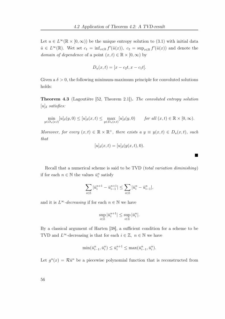
4.2 Application of Theorem 4.2: A TVD-result
Let u ∈ L∞(R × [0,∞)) be the unique entropy solution to (3.1) with initial data
u ∈ L∞(R). Wet set c1 = infx∈R f′(u(x)), c2 = supx∈R f
′(u(x)) and denote the
domain of dependence of a point (x, t) ∈ R× [0,∞) by
Du(x, t) = [x− c2t, x− c1t].
Given a δ > 0, the following minimum-maximum principle for convoluted solutions
holds:
Theorem 4.3 (Lagoutière [52, Theorem 2.1]). The convoluted entropy solution
[u]δ satisfies:
miny∈Du(x,t)
[u]δ(y, 0) ≤ [u]δ(x, t) ≤ maxy∈Du(x,t)
[u]δ(y, 0) for all (x, t) ∈ R× [0,∞).
Moreover, for every (x, t) ∈ R × R+, there exists a y ≡ y(x, t) ∈ Du(x, t), such
that
[u]δ(x, t) = [u]δ(y(x, t), 0).
Recall that a numerical scheme is said to be TVD (total variation diminishing)
if for each n ∈ N the values uni satisfy
∑
i∈Z
|un+1i − un+1
i−1 | ≤∑
i∈Z
|uni − uni−1|,
and it is L∞-decreasing if for each n ∈ N we have
supi∈Z
|un+1i | ≤ sup
i∈Z|uni |.
By a classical argument of Harten [38], a sufficient condition for a scheme to be
TVD and L∞-decreasing is that for each i ∈ Z, n ∈ N we have
min(uni−1, uni ) ≤ un+1
i ≤ max(uni−1, uni ).
Let gn(x) = Run be a piecewise polynomial function that is reconstructed from
56

4 Connecting the Toro-Titarev solver and the LeFloch-Raviart expansion
the cell averages uni i∈Z such that
1
∆x
∫ xi+1/2
xi−1/2
gn(x) dx = uni , and therefore∫
R
gn(x)dx = ∆x∑
i∈Z
uni .
Theorem 4.4 (Lagoutière [52, Proposition 3.2]). Consider a generalized Godunov
scheme with exact numerical flux
fni+1/2 =
1
∆t
∫ ∆t
0
f(
E(τ)gn(xi+1/2))
dτ,
and a suitable CFL-condition. Assume that f ′ > 0. Then the scheme is TVD and
L∞-decreasing (and thus convergent), if the following holds for every i ∈ Z, n ∈ N :
min(uni−1, uni ) ≤ [gn]∆x((i− θ)∆x) ≤ max(uni−1, u
ni ) for all θ ∈ [0, 1]. (4.2)
Proof (As in [52]). Assume that condition (4.2) holds. Note that there are no
transonic waves, since we assumed f ′(u) > 0. Conservativity of the reconstruction
implies that for all i ∈ Z, n ∈ N, we have
uni = [R(
unj j∈Z)
]∆x(xi) = [gn]∆x(xi).
In that case, condition (4.2) reads
min ([gn]∆x(xi−1), [gn]∆x(xi)) ≤ [gn]∆x(xi − θ∆x))
≤ max ([gn]∆x(xi−1), [gn]∆x(xi)) for all θ ∈ [0, 1].
Under the CFL-condition, the domain of dependence of the point (x, t) = (xi,∆t)
is included in the interval [xi−1, xi]. We can view this interval as the set of convex
combinations of xi−1 and xi, so the maximum principle for convoluted solutions
gives
minθ∈[0,1]
[gn]∆x(θxi−1 + (1− θ)xi) ≤ [E(∆t)gn]∆x(xi)
≤ maxθ∈[0,1]
[gn]∆x(θxi−1 + (1− θ)xi).
57

4.2 Application of Theorem 4.2: A TVD-result
So, by condition (4.2), we get
min(uni−1, uni ) ≤ [E(∆t)gn]∆x(xi) ≤ max(uni−1, u
ni ).
Finally, we note that
[E(∆t)gn]∆x(xi) = AjE(∆t)gn(xj) = un+1i ,
and thus
min(uni−1, uni ) ≤ un+1
i ≤ max(uni−1, uni ).
What is remarkable about condition (4.2) is that it imposes a restriction on the
total variation of the sliding averages of the reconstruction,
[gn]∆x(xi − θ∆x) =
∫ xi+1/2−θ∆x
xi−1/2−θ∆x
gn(x) dx, θ ∈ [0, 1],
rather than on the total variation of the reconstruction itself.
A crucial ingredient in the line of reasoning in the above proof is that the new
cell-averages are computed as exact averages of the evolved initial data. Equiva-
lently, this requires that the numerical flux
fnj+1/2 =
1
∆t
∫ ∆t
0
f(E(τ)gn(xi+1/2)) dτ
can be computed exactly. However, this usually is not the case. Instead we assume
that the numerical flux fni+1/2 satisfies
|fni+1/2 − fn
i+1/2| = O(∆tr), ∆t→ 0, i ∈ Z, n ∈ N.
As we have seen, the ADER flux has this property. As an extension of Lagoutière’s
Theorem, we state the following stability result for ADER schemes:
58

4 Connecting the Toro-Titarev solver and the LeFloch-Raviart expansion
Theorem 4.5. Let the assumptions of Lagoutière’s Theorem 4.4 be satisfied but
instead of the exact averaged flux consider the ADER numerical flux. Assume
further that the reconstruction has the property for all i ∈ Z:
sgn(uni−1 − uni ) = sgn(gn(xi−1/2)− gn(xi+1/2)). (4.3)
Then, for ∆t sufficiently small, the ADER scheme is TVD and L∞-decreasing.
Proof. We note that in the case of exact flux computation, the condition
min(uni−1, uni ) ≤ [E(∆t)gn]∆x(xi) ≤ max(uni−1, u
ni ).
may equivalently be expressed as
min(uni−1, uni ) ≤ uni −
∆t
∆x
(
fni+1/2 − fn
i−1/2
)
≤ max(uni−1, uni ).
Now let J := k, k+1, . . . , k+ ℓ ⊆ Z, ℓ ≥ 2 for some k ∈ Z be an index set such
that
uni−1 ≤ uni ≤ uni+1, k + 1 ≤ i ≤ k + ℓ− 1.
The following holds analogously if we alter all the inequalities. We have the con-
dition
uni−1 ≤ un+1i = uni −
∆t
∆x
(
fni+1/2 − fn
i−1/2
)
≤ uni . (4.4)
We want to analyse whether such an estimate still holds if we replace the exact
flux fnj+1/2 by the ADER flux fn,ADER
i+1/2 . We have to check four cases:
a) Both inequalities in (4.4) hold with equality. In this case, the condition
uni−1 = [gn]∆x(xi − θ∆x) = uni , for all θ ∈ [0, 1]
leads to gn ≡ uni on [xj−3/2, xj+1/2] and thus
fn,ADERj+1/2 − fn,ADER
j−1/2 = 0.
59

4.2 Application of Theorem 4.2: A TVD-result
b) Both inequalities in (4.4) hold strictly. We get the condition
uni−1 ≤ uni −∆t
∆x
(
fn,ADERj+1/2 − fn,ADER
j−1/2
)
≤ uni ,
which can be written as
uni−1 ≤ uni −∆t
∆x
(
fni+1/2 − fn
i−1/2 +O(∆tr))
≤ uni , (4.5)
and since both inequalities in (4.4) hold strictly, (4.5) holds for ∆t sufficiently
small.
c) The left inequality in (4.4) holds with equality. We have
uni−1 = uni −∆t
∆x
(
fni+1/2 − fn
i−1/2
)
< uni ,
which implies fni+1/2 − fn
i−1/2 > 0, but small. Then (4.5) holds if
fn,ADERi+1/2 − fn,ADER
i−1/2 ≥ 0 but small. Recall that the ADER flux is given by
fn,ADERj+1/2 =
1
∆t
∫ ∆t
0
f
(
u(xi+1/2, n∆t+) +
r−1∑
k=1
∂ku
∂tk(xj+1/2, n∆t+)
τk
k!
)
dτ.
By a Taylor expansion of f we see that for sufficiently small ∆t the condition
fn,ADERi+1/2 − fn,ADER
i−1/2 ≥ 0
is satisfied, provided we have f(u(xi+1/2, n∆t+)) ≥ f(u(xi−1/2, n∆t+)). Since we
assumed f ′ > 0, this reduces to
u(xi+1/2, n∆t+) ≥ u(xi−1/2, n∆t+).
Recall that the value u(xi+1/2, n∆t+) is given by the Godunov state of the associ-
ated classical Riemann problem with initial data from the extrapolated boundary
values of the reconstruction. Denote the reconstruction in the cell [xi−1/2, xi+1/2]
by gni . Since f ′ > 0, the Godunov states are given by
u(xi+1/2, n∆t+) = gni (xi+1/2), u(xj−1/2, n∆t+) = gni−1(xi−1/2).
60

4 Connecting the Toro-Titarev solver and the LeFloch-Raviart expansion
Thus, a sufficient condition for (4.5) is
gni (xi+1/2) ≥ gni−1(xi−1/2).
d) The right inequality in (4.4) holds with equality. The condition
uni−1 < uni −∆t
∆x
(
fni+1/2 − fn
j−1/2
)
= uni
implies fni+1/2 − fn
i−1/2 = 0. However, we only need
fn,ADERi+1/2 − fn,ADER
i−1/2 ≥ 0, but small,
to get
uni−1 ≤ uni −∆t
∆x
(
fn,ADERi+1/2 − fn,ADER
i−1/2
)
≤ uni .
Again, this only requires gni−1(xi−1/2) < gni (xi+1/2) and ∆t small.
There seems to be no numerical scheme available that uses a high order recon-
struction method which satisfies (4.2) and (4.3). A good starting point could be
data-bounded ENO interpolation (BENO), as developed in [12]. But whether fur-
ther slope-limiting to enforce conditions (4.2) and (4.3) leads to a loss of accuracy,
still needs to be analysed and tested numerically.
4.3 Systems
Naturally, the question arises whether the result of Theorem 4.2 can be extended
to the case of systems. What we have to compare are the coefficient qki∗ and the
Godunov state for the kth spatial derivative in the Toro-Titarev solver. It turns out
that for nonlinear systems the two methods do not yield the same approximation:
Theorem 4.6 (Main result for systems). Consider the generalized Riemann prob-
lem for a strictly hyperbolic m × m system of conservation laws, such that every
characteristic field is either genuinely nonlinear or linearly degenerate. Let the
initial data consist of polynomials uL , uR of degree r− 1 with |uL(0)− uR(0)| > 0
sufficiently small. Assume that the solution contains only shock waves and contact
discontinuities.
61
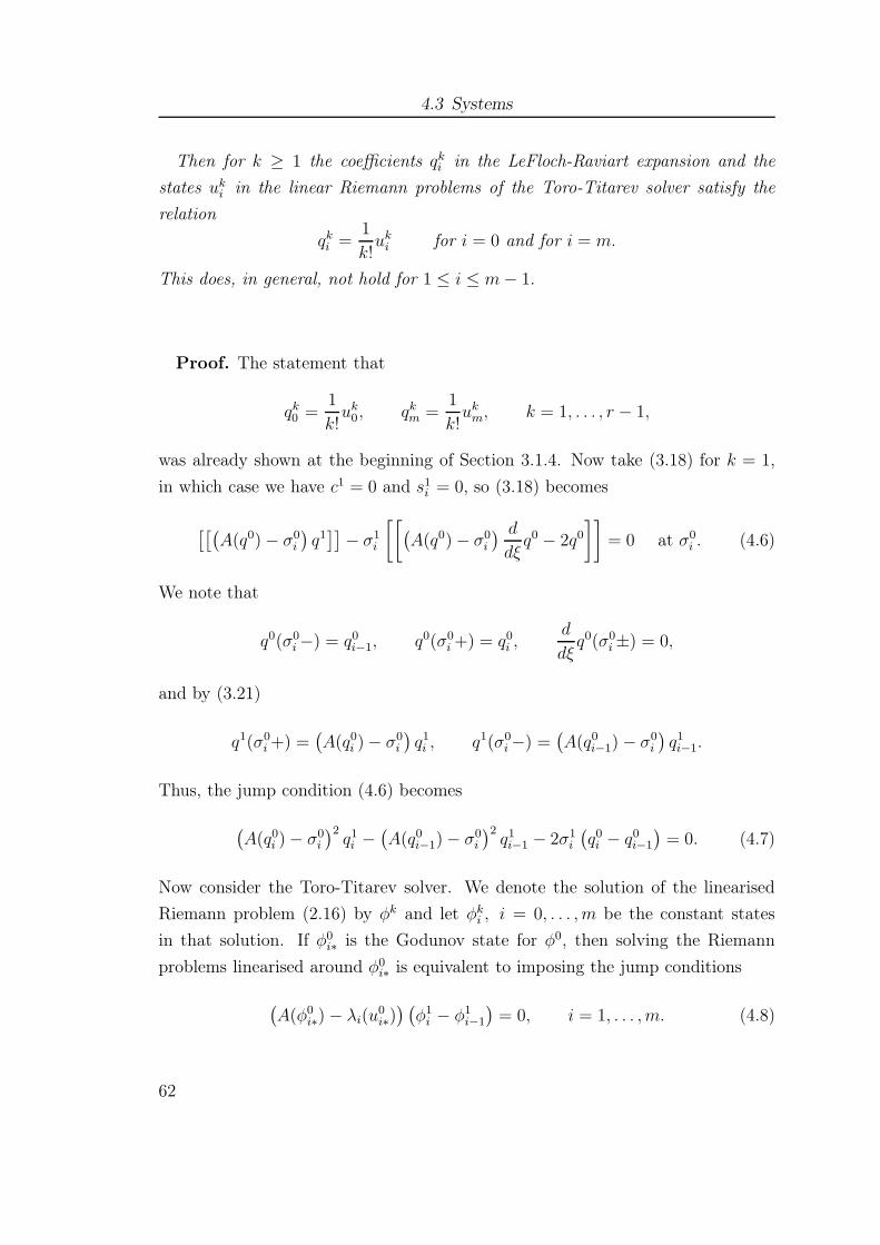
4.3 Systems
Then for k ≥ 1 the coefficients qki in the LeFloch-Raviart expansion and the
states uki in the linear Riemann problems of the Toro-Titarev solver satisfy the
relation
qki =1
k!uki for i = 0 and for i = m.
This does, in general, not hold for 1 ≤ i ≤ m− 1.
Proof. The statement that
qk0 =1
k!uk0, qkm =
1
k!ukm, k = 1, . . . , r − 1,
was already shown at the beginning of Section 3.1.4. Now take (3.18) for k = 1,
in which case we have c1 = 0 and s1i = 0, so (3.18) becomes
[[(
A(q0)− σ0i
)
q1]]
− σ1i
[[
(
A(q0)− σ0i
) d
dξq0 − 2q0
]]
= 0 at σ0i . (4.6)
We note that
q0(σ0i−) = q0i−1, q0(σ0
i+) = q0i ,d
dξq0(σ0
i±) = 0,
and by (3.21)
q1(σ0i+) =
(
A(q0i )− σ0i
)
q1i , q1(σ0i−) =
(
A(q0i−1)− σ0i
)
q1i−1.
Thus, the jump condition (4.6) becomes
(
A(q0i )− σ0i
)2q1i −
(
A(q0i−1)− σ0i
)2q1i−1 − 2σ1
i
(
q0i − q0i−1
)
= 0. (4.7)
Now consider the Toro-Titarev solver. We denote the solution of the linearised
Riemann problem (2.16) by φk and let φki , i = 0, . . . , m be the constant states
in that solution. If φ0i∗ is the Godunov state for φ0, then solving the Riemann
problems linearised around φ0i∗ is equivalent to imposing the jump conditions
(
A(φ0i∗)− λi(u
0i∗)) (
φ1i − φ1
i−1
)
= 0, i = 1, . . . , m. (4.8)
62

4 Connecting the Toro-Titarev solver and the LeFloch-Raviart expansion
Clearly, (4.7) and (4.8) do not have the same solution. An analogous argument
holds in the case k > 1.
We remark, however, that when all states q0i are close, the solutions of (4.7) and
(4.8) are close. This depends only on the leading term q0, but not on higher order
terms. Thus, when the jump in the initial data |u0L − u0R| is small we expect (4.8)
to give a good approximation to (4.7). This explains why the ADER method does
achieve the designed order of accuracy in regions where the solution is smooth,
since in those regions the WENO reconstruction leads to initial data with only
very small jumps.
63


5 Examples and applications
To illustrate the rather technical results form the previous chapters, we provide
several examples. Firstn we solve the generalized Riemann problem for Burgers
equation with piecewise quadratic initial data. In this case the exact solution can
be computed by the method of characteristics and we see that both the Toro-
Titarev solver and the LeFloch-Raviart expansion reproduce the quadratic Taylor
approximation around the origin. Next, we study a system that is inspired by
a model for two component-chromatography. Due to the special eigenstructure
of the system, we can carry out all the computations for first order terms in the
LeFloch-Raviart expansion explicitly. The next two examples are less theoretically
motivated and show that the LeFloch-Raviart expansion can be used in actual nu-
merical computations. We first present numerical tests for shallow water equations
and finally, we study a system from the modelling of traffic flow which has only
linearly degenerate characteristic fields.
5.1 Burgers equation
Consider Burgers equation,
∂
∂tu+
∂
∂x
(
u2
2
)
= 0,
with initial data
u(x, 0) =
uL(x) = x2 + 2x+ 1, x < 0,
uR(x) = 2x2 − 4x+ 2, x > 0.(x, t) ∈ R×[0,∞), u(x, t) ∈ R.
65

5.1 Burgers equation
x
(a)
u(x, 0)
x
(b)
t
x
t
(c)
D1D0
γ(t)
γ(t)
R1
Figure 5.1: (a): Initial data, (b) characteristics, (c) domains of smoothness
We have u0L = 1 < 2 = u0R. Therefore, the classical Riemann problem for the
leading term contains a rarefaction wave. The solution of the generalized Riemann
problem thus is
u(x, t) =
u0(x, t), x/t ≤ γ(t)/t,
x/t, γ(t)/t < x/t < γ(t)/t
u1(x, t), γ(t)/t ≤ x/t.
Using the method of characteristics, we can explicitly compute
u0(x, t) =2t(x+ 1) + 1−
√
4t(x+ 1) + 1
2t2,
u1(x, t) =4t(x− 1) + 1−
√
8t(x− 1) + 1
4t2.
The boundaries of the rarefaction zone are given by the head-characteristic γ(t) =
2t and the tail-characteristic γ(t) = t.
The deceasing initial data uR will lead to the formation of a new shock. It
can be easily checked that characteristics cross for time larger than tF = 1/4. For
sufficiently small time t > 0 we approximate the solution along the t-axis by
u(0, t) ≈ u(0, 0+) +∂
∂tu(0, 0+)t+
∂2
∂t2u(0, 0+)
t2
2.
Note that the t-axis is contained in the domain D0, so in the subsequent analysis
66

5 Examples and applications
we only need to concern the function u0. We have
∂
∂tu0(x, t) =
1− t(x+ 1)(
−3 +√
4t(x+ 1) + 1)
−√
4t(x+ 1) + 1
t3√
4t(x+ 1) + 1,
from which we get
limt→0+
∂
∂tu0(x, t) = −2(x+ 1)3,
∂
∂tu0(0, 0+) = −2, (5.1)
and
∂2
∂t2u0(x, t) =
2t2(x+ 1)2(
4√
4t(x+ 1) + 1− 15)
+ 2t(x+ 1)(
7√
4t(x+ 1) + 1− 10)
t4(4t(x+ 1) + 1)3/2
+3(
√
4t(x+ 1) + 1− 1)
t4(4t(x+ 1) + 1)3/2.
Therefore
limt→0+
∂2
∂t2u0(x, t) = 10(x+ 1)4,
∂2
∂t2u0(0, 0+) = 10. (5.2)
Thus, the Taylor expansion of the exact solution gives
u(0, t) ≈ 1− 2t + 5t2.
We now compute the terms of the LeFloch-Raviart expansion up to the function
q2(ξ). So we construct the approximation
u(x, t) ≈u(0, 0+) + t
(
∂
∂tu(0, 0+) +
∂
∂xu(0, 0+)
(x
t
)
)
+ t2(
1
2
∂2
∂t2u(0, 0+) +
∂2
∂x∂tu(0, 0+)
(x
t
)
+1
2
∂2
∂x2u(0, 0+)
(x
t
)2)
.
Then, q0 is the solution of the Riemann problem
∂
∂tq0 +
∂
∂x
(
(q0)2
2
)
= 0 x ∈ R, t > 0,
67

5.1 Burgers equation
q0(x, 0) =
1, x < 0,
2, x > 0,
in which case q0(ξ) = 1 for all ξ ∈ D0. The function q1 satisfies the ordinary
differential equation
q10 + (1− ξ)d
dξq10 = 0,
and the solution consistent with the initial data is
q10(ξ) = 2(ξ − 1).
Therefore, we have
h2(ξ) = − d
dξ
f ′′(q00)
2(q1(ξ))2 = −4(ξ − 1).
The inhomogeneous equation for q2,
2q20 + (1− ξ)d
dξq20 = −4(ξ − 1),
has the solution q20(ξ) = (ξ − 1)2 − 4(ξ − 1). Thus,
q(ξ, t) ≈ 1 + 2(ξ − 1)t+ ((ξ − 1)2 − 4(ξ − 1))t2,
q(x, t) ≈ x2 + 2x− 6xt + 5t2 − 2t+ 1,
and in particular
q(0, t) ≈ 1− 2t+ 5t2.
Now we use the solver of Toro and Titarev, where we find the leading term
u(0, 0+) by solving
∂
∂tφ0 +
∂
∂x
(
(φ0)2
2
)
= 0 for x ∈ R, t > 0,
φ0(x, 0) =
1, x < 0,
2, x > 0,
68

5 Examples and applications
This gives φ0(0, 0+) = 1. Next, the Cauchy-Kovalevskaya procedure leads to
∂u
∂t= −u∂u
∂x,
∂2u
∂t= 2
(
∂u
∂x
)2
+ u∂2u
∂x2,
∂
∂t
(
∂u
∂x
)
= −(
∂u
∂x
)2
− u∂2u
∂x2, (5.3)
∂
∂t
(
∂2u
∂x2
)
= −3∂u
∂x
∂2u
∂t− u
∂3u
∂x3.
For φ1 = ∂xu and φ2 = ∂2xu, we have the evolution equations
∂φ1
∂t+ φ0∂φ
1
∂x= −
(
φ1)2
and∂φ2
∂t+ φ0∂φ
2
∂x= −3φ1φ2
with the initial conditions
φ1(x, 0) =
u1L = 2, x < 0,
u1R = −4, x > 0,(5.4)
and
φ2(x, 0) =
u2L = 2 x < 0,
u2R = 4 x > 0.(5.5)
We drop the source terms and linearise around φ0(0, 0+) = 1, so that we have
∂φk
∂t+ φ0∂φ
k
∂x= 0 for k = 1, 2,
together with the initial conditions (5.4) and (5.5), respectively. These linear
problems are readily solved, where we find the Godunov states
φ1(0, 0+) = 2 and φ2(0, 0+) = 2.
69

5.2 Two-component chromatography
By the Cauchy-Kovalevskaya procedure (5.3) we get
∂u
∂t(0, 0+) = −φ0(0, 0+)φ1(0, 0+) = −2,
∂2u
∂t2(0, 0+) = 2
(
φ1(0, 0+))2
+ φ0(0, 0+)φ2(0, 0+) = 10,
and thus again we find
u(0, t) ≈ 1− 2t+ 5t2.
5.2 Two-component chromatography
Consider the system
∂
∂t
(
v
w
)
+∂
∂x
(
v(1 + v + w)−1
w(1 + v + w)−1
)
= 0, v, w > 0 (5.6)
and denote u = (v, w)T , u ∈ U = (0,∞) × (0,∞) ⊂ R2. It is inspired by the
analysis of two-component chromatography, as described by Temple [86]. Note
that the chromatography system contains a constant κ ∈ (0, 1) in the second
equation. Since we are more interested in the analysis and less in the modelling,
we have set κ = 1 to simplify matters without changing the structure of the
solution. The solution of the Riemann problem for (5.6) can be found in [14], a
thorough discussion of mathematical models for chromatography is presented in
[71]. This system has a very nice eigenstructure that allows us to carry out all
the computations we need to determine q1 explicitly. We demonstrate analytically
that the difference between φ1∗ and q1∗ only depends on the size of the jump in the
initial states, not on the size of the jump in the derivatives of the initial data.
The Jacobian of the flux is given by
A(v, w) =1
(1 + v + w)2
(
1 + w −v−w 1 + v
)
70

5 Examples and applications
and it has the eigenvalues and (normalized) eigenvectors
λ1(u) =1
(1 + v + w)2, r1(u) =
1√v2 + w2
(
−v−w
)
λ2(u) =1
1 + v + w, r2(u) =
1√2
(
1
−1
)
.
The left eigenvectors, normalized to ℓi(v, w) · rj(v, w) = δij , are
ℓ1(v, w) = −√v2 + w2
v + w
(
1
1
)
, ℓ2(v, w) = −√2
v + w
(
−wv
)
.
Since we have
∇λ1(u) · r1(u) =2√
v2 + w2· v + w
(1 + v + w)3> 0,
∇λ2(u) · r2(u) = 0,
the first characteristic field is genuinely nonlinear and the second characteristic
field is linearly degenerate.
For this system, shock and rarefaction curves coincide in the sense that each
point in the i-Hugoniot set (i = 1, 2) of a given point u− lies on the integral curve
of ri through u−. Due to the simple nature of the eigenvectors, the integral curves
here are straight lines in the space of conserved variables. We can directly compute
R1(ε)(u) = u+ εr1(u), R2(ε)(u) = u+ εr2(u). (5.7)
Both properties - coinciding shock and rarefaction curves and straight line integral
curves - are of particular interest in the analysis of nonlinear hyperbolic systems,
because the simplified structure of the solution allows answers to questions still
open for general hyperbolic system. See the work of Temple [85, 86] for a discussion
of coinciding shock and rarefaction curves. For systems with straight line curves,
Arora and Roe [2] observed only small postshock oscillations in numerical schemes
and conjectured that for system that do not have the straight line property, Go-
dunov and Roe schemes will produce postshock oscillations. Somewhat similar,
71

5.2 Two-component chromatography
w
v
•r1 r2
Figure 5.2: Integral curves for a system from chromatography
though more theoretically motivated, is a result by Bressan and Jenssen [17] who
were able to use the straight line property do establish BV bounds necessary to
prove convergence for the Godunov scheme.
Now consider the Riemann problem with initial data uL = (vL, wL)T , uR =
(vR, wR)T . Then the Riemann solution contains an intermediate state u∗ = (v∗, w∗),
such that(
v∗
w∗
)
=
(
vL
wL
)
+ε1
√
v2L + w2L
(
−vL−wL
)
, (5.8)
(
vR
wR
)
=
(
v∗
w∗
)
+ε2√2
(
1
−1
)
, (5.9)
for some ε1, ε2.
Because the second field is linearly degenerate, we have λ2(u∗) = λ2(uR) and
therefore
v∗ + w∗ = vR + wR. (5.10)
Further, it follows from (5.8) that
vLw∗ = v∗wL (5.11)
72

5 Examples and applications
and that
ε1 =√
(vL)2 + (wL)2 −√
(v∗)2 + (w∗)2.
Combing the two conditions (5.10) and (5.11), we can explicitly compute
v∗ =vL(vR + wR)
vL + wL
, w∗ =wL(vR + wR)
vL + wL
.
Therefore, the wave strength ε1 is
ε1 =
(
1− v2R + w2R
v2L + w2L
)
√
v2L + w2L.
Recall that the type of wave associated with the first characteristic family depends
on the sign of ε1: We get a 1-shock for ε ≤ 0 and a 1-rarefaction for ε1 > 0 (the
second wave is always a contact discontinuity, independent of the sign of ε2).
Thus, if v2R +w2R ≤ v2L+w
2L, the solution contains a 1-shock, a 2-contact discon-
tinuity and is given by
u(x, t) =
uL, x/t < σ1,
u∗, σ1 < x/t < σ2,
uR, σ2 < x/t,
where σ2 = λ2(u∗) = λ2(uR) and the shock speed σ1 can be computed from the
Rankine-Hugoniot conditions:
σ1 =
∫ 1
0
λ1(θu∗ + (1− θ)uL) dθ =1
(1 + vL + wL)(1 + v∗ + w∗).
Now consider the generalized Riemann problem with piecewise linear initial data:
u(x, 0) = u(x) =
uL(x), x > 0,
uR(x), x < 0,
where
uL(x) =
(
vL(x)
wL(x)
)
=
(
v0Lw0
L
)
+ x
(
v1Lw1
L
)
, (5.12)
73

5.2 Two-component chromatography
and
uR(x) =
(
vR(x)
wR(x)
)
=
(
v0Rw0
R
)
+ x
(
v1Rw1
R
)
. (5.13)
Assume that the solution contains a 1-shock. Denote uka = (vka , wka)
T for a =
L,R, k = 0, 1 and let φ0 be the solution of the classical Riemann problem for (5.6)
with initial data u0L, u0R. Denote the intermediate state in that solution by φ0
∗.
Note that λ1(u) > 0, so the Godunov state is u0L.
The simplified problem in the Toro-Titarev solver for the spatial derivatives is
then given by∂
∂tφ1 + ALR
∂
∂xφ1 = 0, x ∈ R, t > 0,
φ1(x, 0) =
(
v(x)
w(x)
)
=
u1L,
u1R,
x < 0,
x > 0.
Here, ALR = A(u0L). This linear problem has the solution
φ1(x, t) = v(
x− λ1(u0L)t)
r1(u0L) + w
(
x− λ2(u0L)t)
r2(u0L).
We express the vectors u1L, u1R in terms of the basis r1(u0L), r2(u0L), i.e.
u1L = α1L,1r1(u
0L) + α1
L,2r2(u0L), u1L = α1
R,1r1(u0L) + α1
R,2r2(u0L).
We have
α1L,1 =−
(
v1L + w1L
)
√
(v0L)2 + (w0
L)2
v0L + w0L
,
α1L,2 =
√2
(
(
v1L + w1L
) w0L
v0L + w0L
− w1L
)
.
Then the intermediate state φ1∗ can be computed as
φ1∗ = α1
L,1r1(u0L) + α1
R,2r2(u0L)
=
(v1R + w1R)
v0Lv0L+w0
L+ (v1L + w1
L)w0
L
v0L+w0L− w1
L
(v1R + w1R − v1L − w1
L)w0
L
v0L+w0L+ w1
L
. (5.14)
74

5 Examples and applications
Now we compare φ1∗ with the vector q11, which the defines the function q1(ξ) in
the LeFloch-Raviart approximation
u(x, t) = q0(ξ) + tq1(ξ) + . . . .
As above, we find q0 by solving the classical Riemann problem with initial states
u0L, u0R and we denote the constant states in that solution by u0L = q00 , q
01, q
02 = u0R.
The function q1(ξ) is given in each domain D0i by
q1(ξ) =(
ξ −A(q0i ))
q1i , 0 ≤ i ≤ 2,
where we express the unknown vectors q1i as
q1i = α1i,1r1(q
0i ) + α1
i,2r2(q0i ).
The coefficients α10,j, α
12,j for j = 1, 2 are determined by the initial data u1L and
u1R respectively, while the remaining coefficients α11,1, α
21,2 are found by solving
a linear 2-by-2 system of algebraic equations that can be derived from the jump
conditions. We arrive at the system (see Lemma 3.3))
(
λ1(q01)− σ0
1
)2ℓ2(q
00) · r1(q01)α1
1,1 +(
λ2(q01)− σ0
1
)2ℓ2(q
00) · r2(q01)α1
1,2
−(
λ2(q00)− σ0
1
)2α10,2
=ℓ2(q
00) · (q01 − q00)
ℓ1(q00) · (q01 − q00)
(
λ1(q01)− σ0
1
)2ℓ1(q
00) · r1(q01)α1
1,1
+(
λ2(q01)− σ0
1
)2ℓ1(q
00) · r2(q01)α1
1,2 +(
λ1(q00)− σ0
1
)2α10,1
(5.15)
75

5.2 Two-component chromatography
(
λ1(q02)− σ0
2
)2ℓ1(q
01) · r1(q02)α1
2,1 +(
λ2(q02)− σ0
2
)2ℓ1(q
01) · r2(q02)α1
2,2
−(
λ1(q01)− σ0
2
)2α11,1
=ℓ1(q
01) · (q02 − q01)
ℓ2(q01) · (q02 − q01)
(
λ1(q02)− σ0
2
)2ℓ2(q
01) · r1(q02)α1
2,1
+(
λ2(q02)− σ0
2
)2ℓ2(q
01) · r2(q02)α1
2,2 +(
λ2(q01)− σ0
2
)2α11,2
(5.16)
Now recall that q00, q01, q
02 are the constant states in the solution of a classical
Riemann problem. Then, by the relations (5.8), (5.9) for the intermediate state
q01, we find
q01 − q00 = ε1r1(q00), q02 − q01 = ε2r2(q
01).
Therefore, by the orthonormality of the eigenvectors, we get
ℓ2(q00) · (q01 − q00) = 0, ℓ1(q
00) · (q01 − q00) = ε1,
ℓ1(q01) · (q02 − q01) = 0, ℓ2(q
01) · (q02 − q01) = ε2.
Noting further that λ2(q01) = λ2(q02) = σ0
2 and that ℓ1 · r2 = 0, the system (5.15),
(5.16) reduces to
(
λ1(q01)− σ0
1
)2ℓ2(q
00) · r1(q01)α1
1,1 +(
λ2(q01)− σ0
1
)2ℓ2(q
00) · r2(q01)α1
1,2
−(
λ2(q00)− σ0
1
)2α10,2 = 0 (5.17)
(
λ1(q02)− σ0
2
)2ℓ1(q
01) · r1(q02)α1
2,1 −(
λ1(q01)− σ0
2
)2α11,1 = 0 (5.18)
Using condition (5.10), v01 + w01 = v02 + w0
2, we have
(
λ1(q02)− σ0
2
λ1(q01)− σ0
2
)2
= 1,
and thus we get from (5.18) that
α11,1 = ℓ1(q
01) · r1(q02)α1
2,1 = −(
v12 + w12
)
√
(v01)2 + (w0
1)2
v02 + w02
. (5.19)
76

5 Examples and applications
Also, we can see that by (5.11), we have
ℓ2(q00) · r1(q01) = −
√2
(v00 + w00)√
(v01)2 + (w0
1)2(w0
0v01 − w0
1v00) = 0.
Moreover, it is straightforward to show that
λ2(q00)− σ0
1
λ2(q01)− σ01
=v01 + w0
1
v00 + w00
=v02 + w0
2
v00 + w00
.
Finally, this yields
α11,2 =
(
v02 + w02
v00 + w00
)2
α10,2 =
√2
(
v02 + w02
v00 + w00
)2(
(v10 + w10)
w00
v00 + w00
− w10
)
. (5.20)
Thus, the coefficient q11 is given by
q11 = α11,1r1(q
01) + α1
1,2r2(q01)
=
(v12 + w12)
v00
v00+w0
0
+(
v02+w0
2
v00+w0
0
)2 (
(v10 + w10)
w00
v00+w0
0
− w10
)
(v12 + w12)
v00
v00+w0
0
−(
v02+w0
2
v00+w0
0
)2 (
(v10 + w10)
w00
v00+w0
0
− w10
)
. (5.21)
Comparing (5.14) and (5.21), we see that the only difference is the factor
(
v02 + w02
v00 + w00
)2
=
( |u0R|1|u0L|1
)2
,
whose size depends on the size of the jump in the initial data, but not on higher
order terms.
77

5.3 Shallow water equations
5.3 Shallow water equations
A widely used model for many environmental and engineering problems are the
shallow water equations, which we present here in their simplest one-dimensional
form:∂
∂t
(
h
hu
)
+∂
∂x
(
hu
hu2 + 12gh2
)
= 0.
Here h denotes the water hight, u the velocity and g is the gravitational constant.
There is an immense list of literature on shallow water equations, we merely men-
tion [58, Chapter 13] for a discussion of the Riemann problem and [90, 93] for an
overview on numerical techniques.
Using the notation from above and introducing v = h, w = uh, this can be
written as∂
∂t
(
v
w
)
+∂
∂x
(
ww2
v+ 1
2gv2
)
= 0.
Note that v denotes the water height, not the velocity. This deviation from stan-
dard notation might be slightly inconvenient, but we are trying to be consistent
with the notation introduced in Chapter 3.
The Jacobian of the flux is
A(v, w) =
(
0 1
−(
wv
)2+ gv 2w
v
)
=
(
0 1
−u2 + gh 2u
)
,
with eigenvalues
λ1 = u−√
gh, λ2 = u+√
gh,
and corresponding eigenvectors
r1 =
(
1
u−√gh,
)
r2 =
(
1
u+√gh,
)
.
Left eigenvectors, normalized to ℓj · ri = δij , are
ℓ1 =1
2√gh
(
u+√gh
−1
)
, ℓ2 = − 1
2√gh
(
u−√gh
−1
)
.
78

5 Examples and applications
We consider the generalized Riemann problem with initial data hL = hR = 1
and
uL(x) = aLx2 + bLx+ cL, uR(x) = aRx
2 + bRx+ cR.
When cR < 0 < cL, this data leads to a solution with two shock waves.
We compare the resulting approximations up to quadratic terms obtained by
the LeFloch-Raviart expansion and the Toro-Titarev solver, respectively. Refer-
ence solutions are obtained by a random choice method (RCM) on a very fine grid
using an exact Riemann solver and van der Corput pseudo random numbers (see
[91, Chapter 7]). We perform three series of tests:
(i) Large jumps in the initial data, fixed derivatives. We fix
aL = 0.02, aR = −0.01 and bL = 0.4, bR = −0.2. We solve the GRP for cR = −1
and cL = 2, 4, 6, respectively. Results are shown in Figure 5.3. Denoting v = h
and w = hu, the plots show the reference solution (thick black line), the LeFloch-
Raviart approximation (blue circles) and the Toro-Titarev approximation (red
crosses) along the line ξ = 0 for times 0 ≤ t ≤ 0.05. The difference in the two
approximations increases with the size of the jump. We observe that the LeFloch-
Raviart approximation is almost identical to the reference solution.
(ii) Large jumps in first derivatives, fixed jump in states. We fix aL =
0.02, aR = −0.01 and cL = 0.2, cR = −0.1, so we have a fixed jump |u0L−u0R| = 0.3.
We let bR = −1 and test for bL = 2, 4, 6, see Figure 5.4. For all test cases both
approximations are very close to the reference solution.
(iii) Large jumps in second derivatives, fixed jump in states. We take
bL = 0.4, bR = 0.1 and cL = 0.2, cR = −0.1. We choose aR = −1 and solve for
aL = 2, 4, 6, respectively. Results are shown in figure 5.5. Again, for all test cases
both approximations are very close to the reference solution.
Let us compare the resulting L1 errors, compared to the reference solution (see
Table 5.3, Table 5.3 shows the relative L1-errors):
For large jumps in the initial states we note that the Toro-Titarev approximation
has a L1-error that is two orders larger than the L1-error of the LeFloch-Raviart
approximation. If the jump in the initial states is small, the order of the size of
79

5.3 Shallow water equations
uL(x) = 0.02x2 + 0.4x+ cL, uR(x) = −0.01x2 − 0.2x− 1
0 0.01 0.02 0.03 0.04 0.051.51
1.515
1.52
1.525
1.53
1.535
t = 0 to 0.05
v al
ong
ξ =
0
v ref (RCM)TT2LFR2
0 0.01 0.02 0.03 0.04 0.05
0.65
0.7
0.75
0.8
t = 0 to 0.05
w a
long
ξ =
0
w ref (RCM)TT2LFR2
(a) cL = 2, |u0L − u0R| = 3
0 0.01 0.02 0.03 0.04 0.051.89
1.895
1.9
1.905
1.91
1.915
t = 0 to 0.05
v al
ong
ξ =
0
v ref (RCM)TT2LFR2
0 0.01 0.02 0.03 0.04 0.05
2.7
2.75
2.8
2.85
2.9
t = 0 to 0.05
w a
long
ξ =
0
w ref (RCM)TT2LFR2
(b) cL = 4, |u0L − u0R| = 5
0 0.01 0.02 0.03 0.04 0.05
2.29
2.3
2.31
2.32
2.33
t = 0 to 0.05
v al
ong
ξ =
0
v ref (RCM)TT2LFR2
0 0.01 0.02 0.03 0.04 0.055.4
5.5
5.6
5.7
5.8
5.9
t = 0 to 0.05
w a
long
ξ =
0
w ref (RCM)TT2LFR2
(c) cL = 6, |u0L − u0R| = 7
Figure 5.3: Two-shock solution for 1-d shallow water: Jumps in the initial states
80

5 Examples and applications
uL(x) = 0.02x2 + bLx+ 0.2, uR(x) = −0.01x2 − x− 0.1
0 0.01 0.02 0.03 0.04 0.051.025
1.03
1.035
1.04
1.045
1.05
t = 0 to 0.05
v al
ong
ξ =
0
v ref (RCM)TT2LFR2
0 0.01 0.02 0.03 0.04 0.05−0.2
−0.1
0
0.1
0.2
t = 0 to 0.05
w a
long
ξ =
0
w ref (RCM)TT2LFR2
(a) bL = 2, |u1L − u1R| = 3
0 0.01 0.02 0.03 0.04 0.050.98
1
1.02
1.04
1.06
1.08
1.1
t = 0 to 0.05
v al
ong
ξ =
0
v ref (RCM)TT2LFR2
0 0.01 0.02 0.03 0.04 0.05−0.4
−0.3
−0.2
−0.1
0
0.1
t = 0 to 0.05
w a
long
ξ =
0
w ref (RCM)TT2LFR2
(b) bL = 4, |u1L − u1R| = 5
0 0.01 0.02 0.03 0.04 0.050.94
0.96
0.98
1
1.02
1.04
1.06
t = 0 to 0.05
v al
ong
ξ =
0
v ref (RCM)TT2LFR2
0 0.01 0.02 0.03 0.04 0.05−0.6
−0.4
−0.2
0
0.2
0.4
t = 0 to 0.05
w a
long
ξ =
0
w ref (RCM)TT2LFR2
(c) bL = 6, |u1L − u1R| = 7
Figure 5.4: Two-shock solution for 1-d shallow water: Jumps in first derivatives
81

5.3 Shallow water equations
uL(x) = aLx2 + 0.4x+ 0.2, uR(x) = −1x2 − 0.2x− 0.1
0 0.01 0.02 0.03 0.04 0.051.04
1.045
1.05
1.055
1.06
t = 0 to 0.05
v al
ong
ξ =
0
v ref (RCM)TT2LFR2
0 0.01 0.02 0.03 0.04 0.050.01
0.02
0.03
0.04
0.05
0.06
t = 0 to 0.05
w a
long
ξ =
0
w ref (RCM)TT2LFR2
(a) aL = 2, |u2L − u2R| = 3
0 0.01 0.02 0.03 0.04 0.051.045
1.05
1.055
1.06
1.065
1.07
t = 0 to 0.05
v al
ong
ξ =
0
v ref (RCM)TT2LFR2
0 0.01 0.02 0.03 0.04 0.05
0.04
0.045
0.05
0.055
0.06
t = 0 to 0.05
w a
long
ξ =
0
w ref (RCM)TT2LFR2
(b) aL = 4, |u2L − u2R| = 5
0 0.01 0.02 0.03 0.04 0.051.04
1.05
1.06
1.07
1.08
1.09
t = 0 to 0.05
v al
ong
ξ =
0
v ref (RCM)TT2LFR2
0 0.01 0.02 0.03 0.04 0.050.04
0.05
0.06
0.07
0.08
t = 0 to 0.05
w a
long
ξ =
0
w ref (RCM)TT2LFR2
(c) aL = 6, |u2L − u2R| = 7
Figure 5.5: Two-shock solution for 1-d shallow water: Jumps in second derivatives
82

5 Examples and applications
‖v − vLFR‖1 ‖w − wLFR‖1 ‖v − vTT‖1 ‖w − wTT‖1[[u0]] = 3 1.893× 10⁻⁶ 7.709× 10⁻⁶ 1.144× 10⁻⁴ 1.095× 10⁻³
[[u0]] = 5 2.380× 10⁻⁶ 1.967× 10⁻⁵ 3.059× 10⁻⁴ 2.703× 10⁻³
[[u0]] = 7 5.061× 10⁻⁶ 4.920× 10⁻⁵ 5.818× 10⁻⁴ 5.340× 10⁻³
[[u1]] = 3 5.935× 10⁻⁶ 2.493× 10⁻⁵ 1.362× 10⁻⁵ 2.923× 10⁻⁴
[[u1]] = 5 1.347× 10⁻⁵ 1.073× 10⁻⁴ 3.136× 10⁻⁵ 1.795× 10⁻⁴
[[u1]] = 7 6.397× 10⁻⁵ 4.727× 10⁻⁴ 8.043× 10⁻⁵ 1.995× 10⁻⁴
[[u2]] = 3 1.670× 10⁻⁶ 2.333× 10⁻⁵ 7.824× 10⁻⁶ 7.538× 10⁻⁵
[[u2]] = 5 2.169× 10⁻⁶ 1.395× 10⁻⁵ 2.005× 10⁻⁶ 3.314× 10⁻⁵
[[u2]] = 7 1.012× 10⁻⁵ 1.987× 10⁻⁵ 3.882× 10⁻⁵ 4.919× 10⁻⁵
Table 5.1: L1-errors for two shock shallow water
‖v−vLFR‖1‖v‖1
‖w−wLFR‖1‖w‖1
‖v−vTT ‖1‖v‖1
‖w−wTT ‖1‖w‖1
[[u0]] = 3 2.499× 10⁻⁵ 2.180× 10⁻⁴ 1.509× 10⁻³ 3.097× 10⁻²
[[u0]] = 5 2.507× 10⁻⁵ 1.421× 10⁻⁴ 3.221× 10⁻³ 1.953× 10⁻²
[[u0]] = 7 4.404× 10⁻⁵ 1.749× 10⁻⁴ 5.062× 10⁻³ 1.898× 10⁻²
[[u1]] = 3 1.150× 10⁻⁴ 6.077× 10⁻³ 2.639× 10⁻⁴ 7.123× 10⁻²
[[u1]] = 5 2.663× 10⁻⁴ 1.467× 10⁻² 6.201× 10⁻⁴ 2.454× 10⁻²
[[u1]] = 7 1.292× 10⁻³ 4.627× 10⁻² 1.624× 10⁻³ 1.953× 10⁻²
[[u2]] = 3 6.225× 10⁻⁵ 1.054× 10⁻¹ 2.280× 10⁻⁴ 1.417× 10⁻¹
[[u2]] = 5 9.696× 10⁻⁵ 7.471× 10⁻² 4.529× 10⁻⁴ 8.483× 10⁻²
[[u2]] = 7 9.665× 10⁻⁵ 5.911× 10⁻² 4.514× 10⁻⁴ 6.712× 10⁻²
Table 5.2: Relative L1-errors for two shock shallow water
83

5.3 Shallow water equations
0 0.01 0.02 0.03 0.04 0.051.35
1.4
1.45
1.5
1.55
t = 0 to 0.05
v al
ong
ξ =
0
v ref (RCM)TT2LFR2
0 0.01 0.02 0.03 0.04 0.05−0.5
0
0.5
1
t = 0 to 0.05
w a
long
ξ =
0
w ref (RCM)TT2LFR2
Figure 5.6: Two-shock solution for 1-d shallow water: Mixed example
the error is the same for both methods.
Now consider an example with large jumps in the states, as well as in first
and second derivatives ( see Figure 5.3). Take uL(x) = 2x2 + 6x + 2, uR(x) =
−x2 − x − 1. We can see that the behaviour we observed for large jumps in the
initial states dominates the behaviour for the approximate solution. The LeFloch-
Raviart approximation is more accurate, although the is a clearly visible error for
larger output times.
Next we turn to a generalized dam-break problem, in which the 1-wave is a
rarefaction wave. Denote the by q00 = (v00 , w00) the left state in the solution of the
classical Riemann problem for the leading term and let
u0 =w0
0
v00, a0 =
√
gv00.
Then solution of the classical Riemann problem inside the 1-rarefaction wave is
given by
q0(ξ) =
(
v0(ξ)
w0(ξ)
)
=1
9g
(
(u0 + 2a0 − ξ)2
13(u0 + 2a0 + 2ξ)(u0 + 2a0 − ξ)2
)
.
This gives
d
dξq0(ξ) = − 2
9g(u0 + 2a0 − ξ)
(
1
ξ
)
, ξ ∈ (σ01, σ
01).
84

5 Examples and applications
For ξ ∈ (σ01, σ
01) we have ξ = λ1(q
0(ξ)) and so it follows that
d
dξq0(ξ) = − 2
9g(u0 + a0 − ξ)
(
1w0(ξ)v0(ξ)
−√
gv0(ξ)
)
= − 2
9g(u0 + 2a0 − ξ)r1
(
q0(ξ))
.
Next we can compute
∇λ1(
q0(ξ))
· dq0(ξ)
dξ=
1
3g(u0 + 2a0 − ξ)
√
gv0(ξ)
v0(ξ).
Moreover, we get
Dr2(
q0(ξ)) dq0(ξ)
dξ= − 2
9g(u0 + 2a0 − ξ)Dr2
(
q0(ξ))
r1(
q0(ξ))
=1
9g(u0 + 2a0 − ξ)
0√gv0(ξ)
v0(ξ)
.
Thus, writing
Dr2(
q0(ξ)) dq0(ξ)
dξ= ω1,2,1r1
(
q0(ξ))
+ ω1,2,2r2(
q0(ξ))
,
we first see that ω1,2,1 = −ω1,2,2 and we compute
ω1,2,2 =u0 + 2a0 − ξ
18gv0(ξ). (5.22)
From (3.30) we get
d
dξαk2 = µk
2 −(
k +∇λ1(q0) · dq0
dξ
λ2(q0)− ξ)+ ω1,2,2
)
αk2 = µk
2 −3k + 2
2(u0 + 2a0 − ξ)αk2.
For k = 1 we have µ12 = 0 and with initial data given by (3.39) the ordinary
85

5.3 Shallow water equations
differential equation for α12 can be solved exactly:
α12(ξ) =
(
σ01 − λ2(q
00))
α10,2
(
u0 + 2a0 − ξ
3a0
)5/2
.
From (3.31) we get
α11(ξ) = − λ2(q
0)− ξ
1 +∇λ1(q0) · dq0
dξ
α12(ξ),
and we first compute
∇λ1(q0) ·dq0
dξ=
1
3g(u0 + 2a0 − ξ)
√gv
v.
Next, recall that for ξ ∈ R01 we have ξ = w0/v0 −
√
gv0 and thus
λ2(q0)− ξ = 2
√
gv0.
Using the fact that ω1,2,1 = −ω1,2,2 we find by (5.22):
α11(ξ) =
u0 + 2a0 − ξ
9√
gv0 + 3(u0 + 2a0 − ξ)α12(ξ).
Finally, note that inside R01 we get
√
gv0(ξ) =1
3(u0 + 2a0 − ξ)
and thus
α11(ξ) =
1
6α12(ξ).
For the quadratic terms, we first note that for f1(v, w) = w all second or higher
86

5 Examples and applications
order derivatives of f1 vanish. Then we get by (3.29) that µ11 = −µ2
2 and
µ22
(
q0, q1)
= − 1
4√
gv0
(
∂3f2(q0)
∂v3dv0
dξ+∂3f2(q
0)
∂v2∂w
dw0
dξ
(v1)2 + 2∂2f2(q
0)
∂v2v1dv1
dξ
+ 2
∂3f2(q0)
∂v2∂w
dv0
dξ
∂3f2(q0)
∂v∂w2
dw0
dξ
v1w1 + 2∂2f2(q
0)
∂v∂w
v1dw1
dξ+ w1dv
1
dξ
+
∂3f2(q0)
∂v∂2w
dv0
dξ+∂3f2(q
0)
∂w3
dw0
dξ
(w1)2 + 2∂2f2(q
0)
∂w2w1dw
1
dξ
)
.
Again, we run three test cases with large jump in the initial states, first derivatives
and second derivatives, respectively. In all three cases we take uL = uR = 0 and
solve the generalized Riemann problem for different piecewise quadratic h. The
ordinary differential equation for α22 is solved numerically, using a classical fourth
order Runge-Kutta method. Results are shown in Figures 5.7-5.9 and the resulting
L1-errors are documented in Tables 5.3 and 5.4.
87

5.3 Shallow water equations
hL(x) = 0.2x2 + 0.2x+ cL, hR(x) = −0.1x2 − 0.1x+ 1
0 0.01 0.02 0.03 0.04 0.051.42
1.43
1.44
1.45
1.46
1.47
t = 0 to 0.05
v al
ong
ξ =
0
v ref (RCM)TT2LFR2
0 0.01 0.02 0.03 0.04 0.051.84
1.86
1.88
1.9
1.92
1.94
t = 0 to 0.05
w a
long
ξ =
0
w ref (RCM)TT2LFR2
(a) cL = 2, |h0L − h0R| = 1
0 0.01 0.02 0.03 0.04 0.052.18
2.185
2.19
2.195
2.2
2.205
2.21
t = 0 to 0.05
v al
ong
ξ =
0
v ref (RCM)TT2LFR2
0 0.01 0.02 0.03 0.04 0.056.95
7
7.05
7.1
7.15
7.2
t = 0 to 0.05
w a
long
ξ =
0
w ref (RCM)TT2LFR2
(b) cL = 4, |h0L − h0R| = 3
0 0.01 0.02 0.03 0.04 0.052.83
2.835
2.84
2.845
2.85
2.855
t = 0 to 0.05
v al
ong
ξ =
0
v ref (RCM)TT2LFR2
0 0.01 0.02 0.03 0.04 0.0513.4
13.45
13.5
13.55
13.6
t = 0 to 0.05
w a
long
ξ =
0
w ref (RCM)TT2LFR2
(c) cL = 6, |h0L − h0R| = 5
Figure 5.7: Generalized dam-break problem: Jumps in the initial states
88

5 Examples and applications
hL(x) = 0.2x2 + bLx+ 3, hR(x) = −0.1x2 − 0.5x+ 2.7
0 0.01 0.02 0.03 0.04 0.052.7
2.75
2.8
2.85
2.9
2.95
t = 0 to 0.05
v al
ong
ξ =
0
v ref (RCM)TT2LFR2
0 0.01 0.02 0.03 0.04 0.050.78
0.8
0.82
0.84
0.86
t = 0 to 0.05
w a
long
ξ =
0
w ref (RCM)TT2LFR2
(a) bL = 0.5, |h1L − h1R| = 1
0 0.01 0.02 0.03 0.04 0.052.6
2.65
2.7
2.75
2.8
2.85
t = 0 to 0.05
v al
ong
ξ =
0
v ref (RCM)TT2LFR2
0 0.01 0.02 0.03 0.04 0.050
0.2
0.4
0.6
0.8
t = 0 to 0.05
w a
long
ξ =
0
w ref (RCM)TT2LFR2
(b) bL = 1.5, |h1L − h1R| = 2
0 0.01 0.02 0.03 0.04 0.05
2.5
2.6
2.7
2.8
2.9
t = 0 to 0.05
v al
ong
ξ =
0
v ref (RCM)TT2LFR2
0 0.01 0.02 0.03 0.04 0.05−0.5
0
0.5
1
t = 0 to 0.05
w a
long
ξ =
0
w ref (RCM)TT2LFR2
(c) bL = 2.5, |h1L − h1R| = 3
Figure 5.8: Generalized dam-break problem: Jumps in first derivatives
89

5.3 Shallow water equations
hL(x) = aLx2 + 0.1x+ 3, hR(x) = −0.5x2 − 0.1x+ 2.7
0 0.01 0.02 0.03 0.04 0.052.81
2.82
2.83
2.84
2.85
2.86
t = 0 to 0.05
v al
ong
ξ =
0
v ref (RCM)TT2LFR2
0 0.01 0.02 0.03 0.04 0.050.78
0.8
0.82
0.84
0.86
0.88
0.9
t = 0 to 0.05
w a
long
ξ =
0
w ref (RCM)TT2LFR2
(a) aL = 0.5, |h2L − h2R| = 1
0 0.01 0.02 0.03 0.04 0.052.835
2.84
2.845
2.85
2.855
t = 0 to 0.05
v al
ong
ξ =
0
v ref (RCM)TT2LFR2
0 0.01 0.02 0.03 0.04 0.05
0.7
0.8
0.9
1
1.1
1.2
1.3
t = 0 to 0.05
w a
long
ξ =
0
w ref (RCM)TT2LFR2
(b) aL = 1.5, |h2L − h2R| = 2
0 0.01 0.02 0.03 0.04 0.052.84
2.85
2.86
2.87
2.88
2.89
t = 0 to 0.05
v al
ong
ξ =
0
v ref (RCM)TT2LFR2
0 0.01 0.02 0.03 0.04 0.05
0.7
0.8
0.9
1
1.1
1.2
1.3
t = 0 to 0.05
w a
long
ξ =
0
w ref (RCM)TT2LFR2
(c) aL = 2.5, |h2L − h2R| = 3
Figure 5.9: Generalized dam-break problem: Jumps in second derivatives
90

5 Examples and applications
‖v − vLFR‖1 ‖w − wLFR‖1 ‖v − vTT‖1 ‖w − wTT‖1[[h0]] = 1 1.640× 10⁻⁵ 5.962× 10⁻⁵ 8.152× 10⁻⁵ 4.197× 10⁻⁴
[[h0]] = 2 3.479× 10⁻⁵ 2.256× 10⁻⁴ 2.909× 10⁻⁴ 2.098× 10⁻³
[[h0]] = 3 4.685× 10⁻⁵ 4.590× 10⁻⁴ 4.617× 10⁻⁴ 4.431× 10⁻³
[[h1]] = 1 6.352× 10⁻⁵ 2.338× 10⁻⁵ 1.118× 10⁻⁴ 3.359× 10⁻⁴
[[h1]] = 2 1.189× 10⁻⁴ 4.043× 10⁻⁴ 3.292× 10⁻⁴ 7.958× 10⁻⁴
[[h1]] = 3 1.841× 10⁻⁴ 1.077× 10⁻³ 6.072× 10⁻⁴ 1.122× 10⁻³
[[h2]] = 1 1.370× 10⁻⁵ 4.299× 10⁻⁵ 2.208× 10⁻⁵ 1.028× 10⁻⁴
[[h2]] = 2 2.963× 10⁻⁵ 3.071× 10⁻⁴ 2.484× 10⁻⁵ 2.456× 10⁻⁴
[[h2]] = 3 8.847× 10⁻⁵ 7.332× 10⁻⁴ 8.216× 10⁻⁵ 6.776× 10⁻⁴
Table 5.3: L1-errors for the generalized dam-break problem
‖v−vLFR‖1‖v‖1
‖w−wLFR‖1‖w‖1
‖v−vTT ‖1‖v‖1
‖w−wTT ‖1‖w‖1
[[u0]] = 3 2.284× 10⁻⁴ 6.410× 10⁻⁴ 1.135× 10⁻³ 4.513× 10⁻³
[[u0]] = 5 3.179× 10⁻⁴ 6.424× 10⁻⁴ 2.658× 10⁻³ 5.947× 10⁻³
[[u0]] = 7 3.306× 10⁻⁴ 6.818× 10⁻⁴ 3.258× 10⁻³ 6.583× 10⁻³
[[u1]] = 3 4.570× 10⁻⁴ 5.943× 10⁻⁴ 8.042× 10⁻⁴ 8.538× 10⁻³
[[u1]] = 5 8.752× 10⁻⁴ 1.813× 10⁻² 2.424× 10⁻³ 3.569× 10⁻²
[[u1]] = 7 1.386× 10⁻³ 7.217× 10⁻² 4.571× 10⁻³ 7.515× 10⁻²
[[u2]] = 3 9.701× 10⁻⁵ 1.042× 10⁻³ 1.563× 10⁻⁴ 2.534× 10⁻³
[[u2]] = 5 2.088× 10⁻⁴ 6.927× 10⁻³ 1.750× 10⁻⁴ 5.539× 10⁻³
[[u2]] = 7 3.273× 10⁻³ 2.027× 10⁻¹ 3.298× 10⁻³ 2.040× 10⁻¹
Table 5.4: Relative L1-errors for the generalized dam-break problem
We observe the same qualitative behaviour as before: When there is a large
jump in the initial data, the Toro-Titarev solver leads to an error which grows
as the jump in the data increases and this error is larger than the error of the
LeFloch-Raviart expansion. If the jump in the initial states is small, the two
approximation methods lead to an error of the same order of magnitude.
91

5.4 A system from traffic flow
5.4 A system from traffic flow
The following system arises in a macroscopic model of traffic flow that was proposed
by Aw and Rascle [3]. It was designed to cure some of the major flaws that previous
models suffered from when attempting to introduce ideas from fluid dynamics to
the world of traffic modelling, see [30]. A detail introduction to conservation law
models in macroscopic traffic flow and further references are found in [69]. We
consider the system
∂
∂tρ+
∂
∂x(ρs) = 0 (5.23)
∂
∂t(s+ p(ρ)) + s
∂
∂x(s+ p(ρ)) = 0.
Here, ρ is the density of cars, s the velocity. The function p acts like a pressure term
in fluid dynamics, but is understood as an ’anticipation factor’. Global existence
and smoothness of the solution to a generalized Riemann problem for (5.23) are
discussed in [84]. We assume ρ > 0 (although the case ρ = 0 can be handled) and
we also assume p′(ρ) > 0, where the specific choice of p will be discussed later.
We can write the system in quasi-linear form,
∂
∂tz + A(z)
∂
∂xz = 0,
where z = (ρ, s)T and
A(z) =
(
s ρ
0 s− ρp′(ρ)
)
.
To derive the correct shock-conditions, we need to rewrite the system in conserva-
tive form. Setting
w = ρ(s+ p(ρ)),
92

5 Examples and applications
the system can be written as
∂
∂tρ+
∂
∂x(ρs) = 0,
∂
∂tw +
∂
∂x(ws) = 0.
Noting that s = w/ρ− p(ρ) we let u = (ρ, w)T and arrive at
∂
∂tu+
∂
∂xf(u) = 0, f(u) =
(
w − ρp(ρ)
w2/ρ− wp(ρ)
)
.
Thus, we have
Df(u) =
(
−p(ρ)− ρp′(ρ) 1
−(w/ρ)2 − wp′(ρ) 2w/ρ− p(ρ).
)
Then the eigenvalues and eigenvectors are
λ1(ρ, w) =w
ρ− p(ρ)− ρp′(ρ), r1(ρ, w) =
(
1wρ
)
,
λ2(ρ, w) =w
ρ− p(ρ) = s, r2(ρ, w) =
(
1wρ+ ρp′(ρ)
)
.
After normalizing to li(ρ, w) · rj(ρ, w) = δij, the left eigenvectors are
ℓ1(ρ, w) =1
ρp′(ρ)
(
wρ+ ρp′(ρ)
−1
)
, ℓ2(ρ, w) =1
ρp′(ρ)
(
−wρ
1
)
.
It is easy to see that the second field is always linearly degenerate, while the first
field is linearly degenerate, if and only if
p(ρ) = a− b
ρ, a, b > 0.
Under this assumption, both waves are contact discontinuities. For actually mod-
elling traffic flow, one usually takes p in the form p(ρ) = ργ , γ > 0. However, for
purposes of analysis and less of modelling, we are interested in a nonlinear system
93

5.4 A system from traffic flow
for which all fields are linearly degenerate. With this choice of p we get
λ1(ρ, w) =w
ρ− a, λ2(ρ, w) =
w + b
ρ− a
and
r1(ρ, w) =
(
1wρ
)
, r2(ρ, w) =
(
1w+bρ
)
,
ℓ1(ρ, w) =1
b
(
w + b
−ρ
)
, ℓ2(ρ, w) =1
b
(
w
−ρ
)
.
The value of w is given by
w = (a+ s)ρ− b.
Since both waves are contact discontinuities, we can compute the Godunov state
from the conditions
λ1(q00) = λ1(q
01), λ2(q
01) = λ2(q
02),
which gives
q01 =
(
ρ01
s01
)
=
(
ρ00b
ρ00(s0
2−s0
0)−b
s02
)
. (5.24)
Next, we present some numerical results considering the generalized Riemann
problem with piecewise constant density ρL and ρR, and piecewise quadratic ve-
locity. We fix a = 0.5, b = 1.
As in the previous section, we compare the resulting approximations up to
quadratic terms obtained by the LeFloch-Raviart expansion and the Toro-Titarev
solve, respectively. Reference solutions are, again, obtained by a random choice
method (RCM) on a very fine grid using an exact Riemann solver and van der
Corput pseudo random numbers. We perform three series of tests:
(i) Large jumps in the initial data, fixed derivatives. We take
ρL(x) = 0.8, ρR(x) = 0.6
and solve the generalized Riemann problem for different choices of sL, sR. Results
94

5 Examples and applications
along the line ξ = 0 for 0 ≤ t ≤ 0.01 are shown in Figure 5.10.
(ii) Large jumps in first derivatives, fixed jump in states Again we take
ρL(x) = 0.62, ρR(x) = 0.6 and choose different sL, sR such that we have small
jumps in the initial states and large jumps in first derivatives, see Figure 5.11.
(iii) Large jumps in second derivatives, fixed jump in states. We fix
ρL(x) = 0.62, ρR(x) = 0.6 and solve the generalized Riemann problem with dif-
ferent sL and sR such that increasing jumps in second derivatives. The results are
shown in Figures and 5.12.
Tables 5.5 and 5.6 show the L1 -errors and relative L1 -errors, respectively. Note
that the errors are measured on the interval [0, 0.01], whereas we took [0, 0.05] for
the shallow water case. Further numerical experiments indicate that the Toro-
Titarev approximation quickly becomes less accurate for larger output times.
Moreover, we need a jump in the initial states of size in the order of 0.01 to
observe the same behaviour as before. If we choose a jump of size 0.1 (as we did in
the shallow water examples), the Toro-Titarev approximations produce an error
two orders larger than the error for the LeFloch-Raviart approximation. We ob-
serve that the accuracy of the Toro-Titarev approximation is very sensitive towards
jumps in the initial data. On the other hand, the LeFloch-Raviart approximations
are in all cases very accurate. This can be explained by the special nature of
the system: Both characteristic fields are linearly degenerated, so the problem is
in some sense "almost linear". Therefore, piecewise quadratic data leads to an
"almost quadratic" solutions and a quadratic Taylor approximation is very accu-
rate. But it is still a nonlinear system, so the Toro-Titarev approximation is not
a Taylor approximation. There are no compression phenomena (as would be the
case for shock waves), and the lack of this stabilizing effect explains the sensitivity
problems.
95

5.4 A system from traffic flow
‖v − vLFR‖1 ‖w − wLFR‖1 ‖v − vTT‖1 ‖w − wTT‖1[[u0]] = 3 4.822× 10⁻⁹ 5.965× 10⁻⁸ 2.921× 10⁻⁶ 1.961× 10⁻⁵
[[u0]] = 5 2.846× 10⁻⁹ 3.922× 10⁻⁸ 3.191× 10⁻⁶ 3.202× 10⁻⁵
[[u0]] = 7 1.739× 10⁻⁹ 3.921× 10⁻⁸ 3.274× 10⁻⁶ 4.378× 10⁻⁵
[[u1]] = 3 1.411× 10⁻⁶ 8.004× 10⁻⁷ 1.319× 10⁻⁶ 2.597× 10⁻⁶
[[u1]] = 5 1.881× 10⁻⁶ 4.712× 10⁻⁷ 1.713× 10⁻⁶ 2.936× 10⁻⁶
[[u1]] = 7 2.866× 10⁻⁶ 4.271× 10⁻⁷ 2.187× 10⁻⁶ 3.286× 10⁻⁶
[[u2]] = 3 1.710× 10⁻⁷ 2.266× 10⁻⁷ 2.057× 10⁻⁷ 4.839× 10⁻⁷
[[u2]] = 5 8.510× 10⁻⁸ 1.291× 10⁻⁷ 1.823× 10⁻⁷ 4.045× 10⁻⁷
[[u2]] = 7 6.574× 10⁻⁸ 9.976× 10⁻⁸ 1.618× 10⁻⁷ 3.737× 10⁻⁷
Table 5.5: L1-errors for traffic flow
‖v−vLFR‖1‖v‖1
‖w−wLFR‖1‖w‖1
‖v−vTT ‖1‖v‖1
‖w−wTT ‖1‖w‖1
[[u0]] = 3 3.038× 10⁻⁶ 1.500× 10⁻⁴ 1.840× 10⁻³ 4.930× 10⁻²
[[u0]] = 5 2.741× 10⁻⁶ 1.507× 10⁻⁴ 3.074× 10⁻³ 1.230× 10⁻¹
[[u0]] = 7 2.254× 10⁻⁶ 2.028× 10⁻⁴ 4.244× 10⁻³ 2.264× 10⁻¹
[[u1]] = 3 2.400× 10⁻⁴ 4.658× 10⁻² 2.243× 10⁻⁴ 1.511× 10⁻¹
[[u1]] = 5 3.176× 10⁻⁴ 2.747× 10⁻² 2.891× 10⁻⁴ 1.712× 10⁻¹
[[u1]] = 7 4.810× 10⁻⁴ 2.474× 10⁻² 3.670× 10⁻⁴ 1.903× 10⁻¹
[[u2]] = 3 2.914× 10⁻⁵ 6.927× 10⁻² 3.505× 10⁻⁵ 1.479× 10⁻¹
[[u2]] = 5 1.448× 10⁻⁵ 3.959× 10⁻² 3.103× 10⁻⁵ 1.240× 10⁻¹
[[u2]] = 7 1.119× 10⁻⁵ 3.058× 10⁻² 2.752× 10⁻⁵ 1.146× 10⁻¹
Table 5.6: Relative L1-errors for traffic low
From what we have a seen for all three examples (shallow water with two shocks
and shallow water with rarefaction and shock, traffic flow with two contact discon-
tinuities) we conclude that the size of the error in the Toro-Titarev approximation
depends mainly on the jump in the initial states. This is consistent with our
analytical results, see the remark after Theorem 4.6.
96

5 Examples and applications
sL(x) = 1/10x2 + 1/10x+ 1/2, sR(x) = −1/10x2 − 1/10x+ cR
0 0.002 0.004 0.006 0.008 0.010.1594
0.1596
0.1598
0.16
0.1602
t = 0 to 0.01
v al
ong
ξ =
0
v ref (RCM)TT2LFR2
0 0.002 0.004 0.006 0.008 0.01−0.045
−0.044
−0.043
−0.042
−0.041
−0.04
−0.039
t = 0 to 0.01
w a
long
ξ =
0
w ref (RCM)TT2LFR2
(a) cR = 33/6, |u0L − u0R|1 = 3
0 0.002 0.004 0.006 0.008 0.010.1036
0.1038
0.104
0.1042
0.1044
t = 0 to 0.01
v al
ong
ξ =
0
v ref (RCM)TT2LFR2
0 0.002 0.004 0.006 0.008 0.01−0.034
−0.032
−0.03
−0.028
−0.026
t = 0 to 0.01
w a
long
ξ =
0
w ref (RCM)TT2LFR2
(b) cR = 53/6, |u0L − u0R|1 = 5
0 0.002 0.004 0.006 0.008 0.010.0765
0.077
0.0775
0.078
0.0785
t = 0 to 0.01
v al
ong
ξ =
0
v ref (RCM)TT2LFR2
0 0.002 0.004 0.006 0.008 0.01−0.028
−0.026
−0.024
−0.022
−0.02
−0.018
t = 0 to 0.01
w a
long
ξ =
0
w ref (RCM)TT2LFR2
(c) cR = 73/6, |u0L − u0R|1 = 7
Figure 5.10: Jumps in the states
97

5.4 A system from traffic flow
sL(x) = 0.5x2 + 0.1x+ 1.1129, sR(x) = −0.1x2 + bRx+ 1.2
0 0.002 0.004 0.006 0.008 0.010.588
0.59
0.592
0.594
0.596
0.598
0.6
t = 0 to 0.01
v al
ong
ξ =
0
v ref (RCM)TT2LFR2
0 0.002 0.004 0.006 0.008 0.01−4
−3
−2
−1
0x 10−3
t = 0 to 0.01
w a
long
ξ =
0
w ref (RCM)TT2LFR2
(a) bR = −4.833, |u1L − u1R|1 = 3
0 0.002 0.004 0.006 0.008 0.01
0.58
0.585
0.59
0.595
0.6
0.605
t = 0 to 0.01
v al
ong
ξ =
0
v ref (RCM)TT2LFR2
0 0.002 0.004 0.006 0.008 0.01−5
−4
−3
−2
−1
0x 10−3
t = 0 to 0.01
w a
long
ξ =
0
w ref (RCM)TT2LFR2
(b) bR = −7.8167, |u1L − u1R|1 = 5
0 0.002 0.004 0.006 0.008 0.01
0.58
0.59
0.6
0.61
0.62
t = 0 to 0.01
v al
ong
ξ =
0
v ref (RCM)TT2LFR2
0 0.002 0.004 0.006 0.008 0.01−5
−4
−3
−2
−1
0x 10−3
t = 0 to 0.01
w a
long
ξ =
0
w ref (RCM)TT2LFR2
(c) bR = −11.15, |u1L − u1R|1 = 7
Figure 5.11: Jumps in first derivatives
98

5 Examples and applications
sL(x) = 0.5x2 + 0.1x+ 1.1129, sR(x) = aRx2 − 0.1x+ 1.2
0 0.002 0.004 0.006 0.008 0.010.588
0.588
0.5881
0.5881
0.5882
0.5882
t = 0 to 0.01
v al
ong
ξ =
0
v ref (RCM)TT2LFR2
0 0.002 0.004 0.006 0.008 0.01−8
−6
−4
−2
0x 10−4
t = 0 to 0.01
w a
long
ξ =
0
w ref (RCM)TT2LFR2
(a) aR = −4.833, |u2L − u2R|1 = 3
0 0.002 0.004 0.006 0.008 0.010.588
0.5881
0.5881
0.5882
0.5882
t = 0 to 0.01
v al
ong
ξ =
0
v ref (RCM)TT2LFR2
0 0.002 0.004 0.006 0.008 0.01−8
−6
−4
−2
0x 10−4
t = 0 to 0.01
w a
long
ξ =
0
w ref (RCM)TT2LFR2
(b) aR = −7.8167, |u2L − u2R|1 = 5
0 0.002 0.004 0.006 0.008 0.010.588
0.5881
0.5881
0.5882
0.5882
t = 0 to 0.01
v al
ong
ξ =
0
v ref (RCM)TT2LFR2
0 0.002 0.004 0.006 0.008 0.01−8
−6
−4
−2
0x 10−4
t = 0 to 0.01
w a
long
ξ =
0
w ref (RCM)TT2LFR2
(c) aR = −11.15, |u2L − u2R|1 = 7
Figure 5.12: Jumps in second derivatives
99


6 Conclusion and outlook
We have shown that the Toro-Titarev solver computes a truncated Taylor-Series
expansion when applied to a scalar problem. We used this insight to extend a
stability result that used exact flux computation to the case of the ADER numerical
flux. It seems likely that more results in this direction are possible. Moreover, if
we take any entropy - entropy flux pair Q, F and define a numerical entropy flux
by Fi+1/2 =∫ ∆t
0F (u(xi+1/2, t)) dt, this approximation result could play a mayor
role in proving entropy stability of the numerical scheme.
For nonlinear systems we have shown that the Toro-Titarev solver does not
compute a Taylor expansion. The resulting approximation does, in general, not
satisfy the Rankine-Hugoniot conditions. However, the error is small, provided the
jump in the initial states is small. Whether the LeFloch-Raviart expansion, which
gives more accurate approximations in the case of large jumps, could be used with
higher orders at a competitive computational cost, remains to be tested.
We based our analysis on the assumption that the system is strictly hyperbolic
with only genuinely nonlinear or linearly degenerate characteristic fields. While
this assumption does cover many systems of practical interest, it leaves out a broad
set of problems. The Riemann problem can be solved for a lot of systems that are
not strictly hyperbolic or for which some characteristic fields are neither genuinely
nonlinear nor linearly degenerate. If we view the generalized Riemann problem
locally as a perturbation of a classical Riemann problem, it seems reasonable that
the generalized Riemann problem should also have a solution in these cases and a
similar asymptotic analysis as in our case is possible. However, if we want to do
this there is still a large amount of highly technical work ahead of us.
We did not analyse the effects of using approximate Riemann solvers for the
leading term Riemann problem. It is one of the advantages of the Toro-Titarev
solver that an approximate solution of the generalized Riemann problem can be
101

computed once the (approximate) Godunov state of the leading term Riemann
problem is known. On the other hand, the LeFloch-Raviart expansion requires a
full Riemann solver. Approximate solutions of the leading term Riemann problem
could be used, but the method needs all intermediate states and all waves speeds
in the classical Riemann problem.
Problems in several spatial dimensions are most important in applications but
extremely hard to analyse. Local generalised Riemann problems at the cell-
boundaries are essentially one-dimensional and can be handled using the approach
described by Harabetian [37]. However, at the corners of the cells, where more
than two cells meet, a very rich variety of wave interactions is to be expected.
This is already true for the classical Riemann in two dimension and it seems like
there are no results on the piecewise smooth case available yet.
102

Bibliography
[1] T. Aboiyar, E. Georgoulis, and A. Iske, Adaptive ADER methodsusing kernel-based polyharmonic spline WENO reconstruction, SIAM J. Sci.Comput., 32 (2010), pp. 3251 – 3277.
[2] M. Arora and P. Roe, On postshock oscillations due to shock capturingschemes in unsteady flows, J. Comput. Phys., 130 (1997), pp. 25–140.
[3] A. Aw and M. Rascle, Resurrection of second order models of traffic flow,SIAM J. Appl. Math., 60 (2000), pp. 916–938.
[4] D. S. Balsara, C. Meyer, M. Dumbser, H. Du, and Z. Xu, Effi-cient implementation of ADER schemes for Euler and mandmagnetohydro-dynamical flows on structured meshes - Speed comparison with Runge-Kuttamethods, J. Comput. Phys., 235 (2013), pp. 934 – 969.
[5] D. S. Balsara, T. Rumpf, M. Dumbser, and C.-D. Munz, Ef-ficient, high order accuracy ADER-WENO schemes for hydrodynamicsand divergence-free magnethydrodynamics, J. Comput. Phys., 228 (2009),pp. 2480 – 2516.
[6] D. S. Balsara and C.-W. Shu, Monotonicity preserving weighted es-sentially non-oscillatory schemes of increasingly high order of accuracy, J.Comput. Phys., 160 (2000), pp. 405–452.
[7] M. Ben-Artzi and J. Falcovitz, A second-oder Godunov type schemefor compressible fluid dynamics, J. Comput. Phys., 55 (1984), pp. 1–32.
[8] , Generalized Riemann Problems in Computational Fluid Dynamics,Cambridge University Press, Cambridge, 2003.
[9] M. Ben-Artzi, J. Falcovitz, and J. Li, The convergence of the GRPscheme, Discrete Contin. Dyn. Syst., 23 (2009), pp. 1–27.
[10] M. Ben-Artzi and J. Li, Hyperbolic balance laws: Riemann invariantsand the generalized Riemann problem, Numer. Math., 106 (2007), pp. 369 –425.
103

Bibliography
[11] M. Ben-Artzi, J. Li, and G. Warnecke, A direct Eulerian GRP schemefor compressible fluid flow, J. Comput Phys., 218 (2006), pp. 19 – 43.
[12] M. Berzins, Nonlinear data-bounded polynomial approximations and theirapplications in ENO methods, Numer. Algor., 55 (2010), pp. 171–189.
[13] A. Bourgeade, P. LeFloch, and P. Raviart, An asymptotic expansionfor the solution of the generalized Riemann problem. Part 2: Application tothe equations of gas dynamics, Ann. Inst. H. Poincare Anal. Non Linéaire, 6(1989), pp. 437 – 480.
[14] A. Bressan, Hyperbolic systems of conservation laws. The one-dimensionalCauchy problem, Oxford University Press, Oxford, 2000.
[15] , The front tracking method for systems of conservation laws, in Hand-book of Differential Equations. Evolution Equations, C. M. Dafermos andE. Feireisl, eds., vol. I, Elsevier, Amsterdam, 2004, pp. 87 – 168.
[16] , BV solutions to Hyperbolic Systems by Vanishing Viscosity, in Hyper-bolic Systems of Balance Laws, P. Marcati, ed., vol. 1911 of Lecture Notesin Mathematics, Springer, Berlin, 2007, pp. 1–77.
[17] A. Bressan and H. Jenssen, On the convergence of Godunov scheme fornonolinear hyperbolic conservation laws, Chines Ann. Math. - B, 21 (2000),pp. 1–16.
[18] A. Bressan and P. LeFloch, Structural stability and regularity of entropysolutions to hyperbolic systems of conservation laws, Indiana U. Math. J., 48(1999), pp. 43 – 84.
[19] C. E. Castro and E. F. Toro, Solvers for the high-order Riemann prob-lem for hyperbolic balance laws, J. Comput. Phys., 227 (2008), pp. 2481 –2513.
[20] S. Chen, X. Han, and H. Zhang, The generalized Riemann problem forfirst order quasilinear hyperbolic systems of conservation laws II, Acta Appl.Math., 108 (2009), pp. 235–277.
[21] S. Chen, D. Huang, and X. Han, The generalized Riemann problem forfirst order quasilinear hyperbolic systems of conservation laws I, Bull. KoreanMath. Soc., 46 (2009), pp. 409–434.
[22] A. J. Chorin, Random choice solutions of hyperbolic systems, J. Comput.Phys., 22 (1976), pp. 517 – 533.
104

Bibliography
[23] P. Colella, Glimm’s method for gas dynamics, SIAM J. Sci. Stat. Com-put., 3 (1982), pp. 76 – 110.
[24] P. Colella and P. Woodward, The Piecewise Parabolic Method (PPM)for gas-dynamical simulations, J. Comput. Phys., 54 (1984), pp. 174–201.
[25] F. Coquel and P. G. LeFloch, Convergence of finite difference schemesfor conservation laws in several spatial dimensions: A general theory, SIAMJ. Numer. Anal., 30 (1993), pp. 675 – 700.
[26] , An entropy satisfying MUSCL scheme for systems of conservation laws,Numer. Math., 71 (1996), pp. 1 – 33.
[27] R. Courant, K. Friedrichs, and H. Lewy, Über die Differenzengle-ichungen der mathematischen Physik, Math. Annal., 100 (1928), pp. 32 –74.
[28] C. Dafermos, Generalized characteristics and the structure of solutions ofhyperbolic conservation laws, Indiana Univ. Math. J, 26 (1977), pp. 1097–1119.
[29] , Hyperbolic Conservation Laws in Continuum Physics, Springer, Hei-delberg, 3 ed., 2010.
[30] C. F. Daganzo, Requiem for second-order fluid approximations of trafficflow, Transportation Res. B, 29 (1995), pp. 277 – 286.
[31] R. J. DiPerna, Measure-valued solutions to conservation laws, Arch. Rat.Mech. Anal., 88 (1985), pp. 27 – 70.
[32] L. C. Evans, Weak Convergence Methods for Nonlinear Partial DifferentialEquations, vol. 74 of C.B.M.S., Amer. Math. Soc., 1990.
[33] L. C. Evans and R. Gariepy, Measure theory and fine properties of func-tions, CRC Press, Boca Ranton, 1992.
[34] B. Giacomazzo and L. Rezolla, The exact solution of the Riemannproblem in relativistic magnetohydrodynamics, J. Fluid. Mech., 562 (2006),pp. 223 – 259.
[35] J. Glimm, Solutions in the large for nonlinear hyperbolic systems of conser-vation laws, Comm. Pure. Appl. Math., 18 (1965), pp. 697 – 715.
[36] S. K. Godunov, A difference scheme for numerical solution of discontinu-ous solution of hydrodynamic equations, Math. Sbornik, 47 (1959), pp. 271– 306 (English translation US Joint Publ. Res. Service, JPRS 7226, 1969).
105

Bibliography
[37] E. Harabetian, A convergent series expansion for hyperbolic conservationlaws, tech. rep., NASA Contractor Report 172557, ICASE Report No. 85-13,1985.
[38] A. Harten, On a class of high resolution total-variation-stable finite-difference schmes, SIAM J. Numer. Anal., 21 (1984), pp. 1–23.
[39] A. Harten, B. Engquist, S. Osher, and S. R. Chakravarthy, Uni-formly high order essentially non-oscillatory schemes, III, J. Comput. Phys.,77 (1987), pp. 231–303.
[40] A. Hidalgo and M. Dumbser, ADER schemes for nonlinear systemsof stiff advection-diffusion-reaction equations, J. Sci. Comput., 48 (2011),pp. 173 – 189.
[41] H. Holden and N. H. Risebro, Front Tracking for Hyperbolic Conserva-tion Laws, Springer, New York, 2002.
[42] J. M. Hong and P. G. LeFloch, A version of the Glimm method based ongeneralized Riemann problems, Portugaliae Mathematica, 64 (2007), pp. 199– 236.
[43] L. Hörmander, Lecture Notes on Nonlinear Hyperbolic Differential Equa-tions, Springer, Berlin, Heidelberg, 1997.
[44] G.-S. Jiang and C.-W. Shu, Efficient implementation of weighted essen-tially non-oscillatory schemes, J. Comput. Phys., 126 (1996), pp. 202–212.
[45] F. John, Formation of singularities in one-dimensional nonlinear wavepropagation, Comm. Pure Appl. Math., 23 (1974), pp. 377–405.
[46] M. Käser and A. Iske, ADER schemes on adaptive triangular meshes forscalar conservation laws, J. Comput. Phys., 205 (2005), pp. 486 – 508.
[47] V. P. Kolgan, Application of the principle of minimum derivatives to theconstruction of difference schemes for computing discontinuous solutions ofgas dynamics (in Russian), Uch. Zap. TsaGI, Russia, 3 (1972), pp. 68 –77 (Reprinted and translated in: J. Comput. Phys., 230 (2011), pp. 2384 –2390).
[48] D.-X. Kong, Global structure stability of Riemann solutions of quasilinearhyperbolic systems of conservation laws: Shocks and contact discontinuities,J. Differential Equations, 188 (2003), pp. 242–271.
106

Bibliography
[49] , Global structure instability of Riemann solutions of quasilinear hyper-bolic systems of conservation laws: Rarefaction waves, J. Differential Equa-tions, 219 (2005), pp. 421–450.
[50] D. Kröner, Numerical Schemes for Conservation Laws, Wiley / Teubner,Chichester / Stuttgart, 1997.
[51] S. Kruzkov, First-oder quasilinear equations with serveral space variables(in Russian), Mat. Sbornik, 123 (1970), pp. 228 – 255 (English translation:USSR Math. Sbornik 10 (1970), pp. 217 –273).
[52] F. Lagoutiére, Stability of reconstruction schemes for scalar hyperbolicconservation laws, Comm. Math. Sci., 6 (2008), pp. 55–70.
[53] P. Lax, Hyperbolic systems of conservation laws, II, Comm. Pure Appl.Math., 10 (1957), pp. 537–556.
[54] P. Lax and B. Wendroff, Systems of conservation laws, Comm. PureAppl. Math., 13 (1960), pp. 217–237.
[55] P. LeFloch, Hyperbolic Systems of Conservation Laws. The Theory ofClassical and Nonclassical Shock Waves, Birkhäuser Verlag, Basel, 2002.
[56] P. LeFloch and P. A. Raviart, An asymptotic expansion for the solutionof the generalized Riemann problem. Part I: General theory, Ann. Inst. H.Poincare Anal. Non Linéaire, 5 (1988), pp. 179–207.
[57] P. LeFloch and L. Tastien, A global asymptotic expansion for the so-lution to the generalized Riemann problem, IMA Preprint Series, No. 585,(1989).
[58] R. J. LeVeque, Finite Volume Methods for Hyperbolic Problems, Cam-bridge University Press, New York, 2002.
[59] T. Li and W. Yu, Boundary value problems for quasilinear hyperbolic sys-tems, Duke University Press, Durham, NC, 1985.
[60] T.-P. Liu, The deterministic version of the Glimm scheme, Comm. Math.Phys., 57 (1977), pp. 135 – 148.
[61] X.-D. Liu, S. Osher, and T. Chan, Weighted essentially non-oscillatoryschemes, J. Comput. Phys., 115 (1994), pp. 200–212.
[62] J. Málek, J. Necas, M. Rokyta, and M. Růzicka, Weak and Measure-Valued Solutions to Evolutionary PDEs, Chapman & Hall, London, 1996.
107

Bibliography
[63] G. Marshall and R. Méndez, Computational aspects of the randomchoice method for shallow water equations, J. Comput. Phys., 39 (1981),pp. 1 – 21.
[64] I. S. Men’shov, Increasing the order of approximation of Godunov’s schemeusing the solution of the generalized Riemann problem, USSR Comput. Math.Phys., 30 (1990), pp. 54 – 65.
[65] G. Montecinos, C. E. Castro, M. Dumbser, and E. F. Toro, Com-parison of solvers for the generalized Riemann problem for hyperbolic systemswith source terms, J. Comput. Phys., 231 (2012), pp. 6472 – 6494.
[66] K. W. Morton and T. Sonar, Finite volume methods for hyperbolic con-servation laws, Acta Numerica, 16 (2007), pp. 155 – 238.
[67] H. Nessyahu, E. Tadmor, and T. Tassa, The convergence rate of Go-dunov type schemes, SIAM J. Numer. Anal., 31 (1994), pp. 1 – 16.
[68] O. A. Oleinik, Discontinuous solutions of non-linear differential equations(in Russian), Uspehi Math. Nauk (N.S.), 12 (1957), pp. 3 – 73 (Englishtranslation: AMS Transl., Ser. 2, 26, 95–172).
[69] B. Piccoli and M. Garavello, Traffic Flow on Networks - Conserva-tion Laws Models, vol. 1 of AIMS on Applied Math., American Institute ofMathematical Science, 2006.
[70] J.-M. Qui and C.-W. Shu, Convergence of Godunov-type schemes forscalar conservation laws under large time steps, SIAM J. Numer. Anal., 46(2008), pp. 2211 – 2237.
[71] K.-H. Rhee, R. Aris, and N. R. Amnundson, First Oder Partial Dif-ferential Equations, Vol. I-II, Prentice Hall, Engelwood Cliffs, 1986-1989.
[72] B. Riemann, Über die Fortpflanzung ebener Luftwellen von endlicherSchwingungsweite, Abhandlungen der Königlichen Gesellschaft der Wis-senschaften in Göttingen, 8 (1860), pp. 43–66.
[73] T. Schwarzkopff, C. D. Munz, and E. F. Toro, ADER: High-orderapproach for linear hyperbolic systems in 2D, J. Sci. Comput., 17 (2002),pp. 231 – 240.
[74] D. W. Schwendemann, C. W. Wahle, and A. K. Kapila, The Rie-mann problem and a high-resolution Godunov method for a model of com-pressible two-face flow, J. Comput. Phys., 212 (2006), pp. 490 – 526.
108

Bibliography
[75] D. Serre, Systems of Conservation laws 1. Hyperbolicity, Entropies, ShockWaves, Cambridge University Press, Cambridge, 1999.
[76] Z.-Q. Shao, Global structure instability of Riemann solutions for generalquasilinear hyperbolic systems of conservation laws in the presence of aboundary, J. Math. Anal. Appl., 330 (2007), pp. 511–540.
[77] J. Shi, C. Hu, and C.-W. Shu, A technique for treating negative weightsin WENO schemes, J. Comput. Phys., 175 (2002), pp. 108 – 127.
[78] M. Shinbrot and R. Welland, The Cauchy-Kowalewskaya theorem, J.Math. Anal. App., 55 (1976), pp. 757 – 772.
[79] C.-W. Shu, High order weighted essentially non-oscillatory schemes for con-vection dominated problems, SIAM Review, 51 (2009), pp. 82–126.
[80] J. Smoller, Shock waves and reaction-diffusion equations, Springer, NewYork, 1983.
[81] A. Szepessy, Convergence of a shock-capturing streamline diffusion finite el-ement methods for a scalar conservation law in two space dimensions, Math.Comput., 53 (1989), pp. 527 – 545.
[82] E. Tadmor, Approximate solutions of nonlinear conservation laws, inAdvanced Numerical Approximation of Nonlinear Hyperbolic Equations,A. Quarteroni, ed., vol. 1697 of Lecture Notes in Mathematics, Springer,Berlin, 1998, pp. 1 – 149.
[83] , Entropy stability theory for difference approximations of nonlinearconservation laws and related time-dependent problems, Acta Numerica, 12(2003), pp. 451 – 512.
[84] L. Tatsien and W. Libin, Global Propagation of Regular Nonlinear Hy-perbolic Waves, Brikhäuser, Boston, 2009.
[85] B. Temple, Systems of conservation laws with coinciding shock and rar-efaction curves, Contemp. Math., 17 (1983), pp. 143 – 151.
[86] , Systems of conservation laws with invariant submanifolds, Trans.Amer. Math. Soc., 280 (1983), pp. 781 – 795.
[87] V. A. Titarev and E. F. Toro, ADER: Arbitrary high order Godunovapproach, J. Sci. Comput., 17 (2002), pp. 609–618.
109

Bibliography
[88] , ADER schemes for three-dimensional non-linear hyperbolic systems, J.Comput. Phys., 204 (2005), pp. 715–736.
[89] , Analysis of ADER and ADER-WAF schemes, IMA J. Numer. Anal.,27 (2007), pp. 616–630.
[90] E. F. Toro, Shock-Capturing Methods for Free-Surface Shallow Flows, JohnWiley & Sons, Chichester, 2001.
[91] , Riemann Solvers and Numerical Methods for Fluid Dynamics. A Prac-tical Introduction, Springer, Berlin, 3. ed., 2009.
[92] , The Riemann problem in computational science, in Numerical Methodsfor Hyperbolic Equations: Theory and Applications. An international con-ference to honour Professor E. F. Toro, M. E. Vásques-Cedón, A. Hidalgo,P. García-Navarro, and L. Cea, eds., Taylor-Francis Group, 2013, pp. 87 –106.
[93] E. F. Toro and P. Garcia-Navarro, Godunov-type methods for free-surface shallow flows: A review, J. Hydraulic Research, 45 (2007), pp. 736 –751.
[94] E. F. Toro and A. Hidalgo, ADER finite volume schemes for nonlinearreaction-diffusion equations, Appl. Numer. Math., 59 (2009), pp. 73 – 100.
[95] E. F. Toro, R. C. Millington, and L. A. M. Nejad, Towards very highorder Godunov schemes, in Godunov Methods. Theory and Applications,E. F. Toro, ed., Kluwer/Plenum Academic Publishers, 2001, pp. 907 – 940.
[96] E. F. Toro and V. A. Titarev, ADER schemes for scalar hyperbolicconservation laws with source terms in three space dimensions, J. Comput.Phys., 202 (2005), pp. 196 – 215.
[97] , TVD fluxes for the high-order ADER schemes, J. Sci. Comput., 24(2005), pp. 285–309.
[98] , Derivative Riemann solvers for systems of conservation laws andADER methods, J. Comput. Phys., 212 (2006), pp. 150–165.
[99] B. van Leer, Towards the ultimate conservative difference scheme. IV:A second order sequel to Godunov’s method, J. Comput. Phys., 32 (1979),pp. 101–136.
[100] J. P. Vila, An analysis of a class of second-order accurate Godunov-typeschemes, SIAM J. Numer. Anal., 26 (1989), pp. 830 – 853.
110

Bibliography
[101] A. I. Volpert, The spaces BV and quasilinear equations (in Russian), Mat.Sbornik, 73 (1967), pp. 255 – 302 (English translation: Math. USSR Sbornik,2, (1967), pp. 225 – 267 ).
[102] Z. Yang, P. He, and H. Tang, A direct Eulerian GRP scheme for rela-tivistic hydrodynamics: One-dimensional case, J. Comput. Phys., 230 (2011),pp. 7964 – 7987.
[103] K. Yosida, Functional Analysis, 5th Ed., Springer, Berlin, Heidelberg, 1978.
[104] E. C. Zachmanoglou and D. Thoe, Introduction to Partial DifferentialEquations with Applications, Williams & Wilkins, Baltimore, 1976.
[105] X. Zhang and C.-W. Shu, A genuinely high order total variation dimin-ishing scheme for one-dimensional scalar conservation laws, SIAM J. Numer.Anal., 48 (2010), pp. 772 – 795.
[106] , On maxiumum-principle-satisfying high order schemes for scalar con-servation laws, J. Comput. Phys., 229 (2010), pp. 3091 – 3120.
[107] , Maximum-principle-satisfying and positivity-preserving high-orderschemes for conservation laws: survey and new developments, Proc. R. Soc.A, 467 (2011), pp. 2752 – 2776.
[108] W. Ziemer, Weakly differentiable functions: Sobolev spaces and functionsof bounded variation, Springer, New York, 1989.
111


Zusammenfassung
Wir untersuchen die analytischen Eigenschaften von Methoden zur näherungswei-sen Lösung von verallgemeinerten Riemann-Problemen. Dabei konzentrieren wiruns auf den Toro-Titarev-Löser [98], der den zentralen Baustein zur Flussberech-nung in ADER Finite Volumen Methoden zur numerischen Lösung von hyperboli-schen Erhaltungsgleichungen darstellt. Toro und Titarev schlagen vor, die Lösungdes verallgemeinerten Riemann-Problems durch eine Taylor-Reihe zu approximie-ren. Die Koeffizienten der Taylor-Polynome werden in der Methode von Toro undTitarev mit Hilfe einer Cauchy-Kowalewskaya-Prozedur und einer Folge von klas-sischen Riemann-Problemen berechnet.
Diese Strategie zur Berechnung von Näherungslösungen für verallgemeinerteRiemann-Probleme erzielt in einer Vielzahl von Anwendungen sehr gute nume-rische Resultate, eine gründliche analytische Untersuchung des Verfahrens stehtallerdings noch aus. Insbesondere wurde beobachtet, dass ADER-Verfahren fürglatte Lösungen die erwartete Genauigkeitsordnug erreichen, bei großen Sprüngenin den Anfangsdaten aber auf Probleme stoßen [19, 65]. Dieses Phänomen konntebisher nicht erklärt werden.
Wir untersuchen den Toro-Titarev-Löser, indem wir ihn mit einer asymptoti-schen Reihenentwicklung für die Lösung des verallgemeinerten Riemann-Problemsvergleichen, die von LeFloch und Raviart konstruiert wurde [56]. Es stellt sichheraus, dass beide Methoden formell die selbe Taylor-Approximation konstruierenund sich nur in der Berechnung der Ortsableitungen im Ursprung unterscheiden.
Wir zeigen, dass beide Methoden für skalare 1D Probleme zur selben Näherungs-lösung führen. Für nichtlineare Systeme von hyperbolischen Erhaltungsgleichungenergibt sich ein Unterschied. Wir zeigen analytisch, dass dieser Unterschied direktvon der Größe des Sprungs in den Anfangsdaten abhängt und dass der Unterschiedklein ist, wenn der Sprung in den Anfangsdaten klein ist.
Wir illustrieren diesen Sachverhalt, indem wir analytische Resultate für BurgersGleichung und für ein System aus der Zwei-Komponenten Chromatographie be-reitstellen. Weitere numerische Resultate für Flachwassergleichungen und für einSystem aus der Verkehrsflussmodellierung bestätigen die analytischen Resultate.

Abstract
We study the analytical properties of approximate solvers for the generalized Rie-mann problem. We focus on the Toro-Titarev solver [98], which is the heart ofthe flux computation in ADER finite volume methods for solving hyperbolic con-servation laws. Toro and Titarev suggested to approximate the solution of thegeneralized Riemann problem by a truncated Taylor series expansion. Coefficientsin this expansion are found using a Cauchy-Kovalevskaya procedure and a sequenceof classical Riemann problems.
This method for approximately solving the generalized Riemann problem hasbeen applied successfully to a wide range of problems, but few rigorous analysisof this strategy has been reported so far. It was observed that the ADER schemeachieves the designed order of accuracy in regions where the solution is smooth,but can encounter difficulties if the initial data contains large jumps [19, 65]. Thisphenomenon has thus far not been explained.
We study the solver of Toro and Titarev by comparing it to a local asymptoticseries expansion for the solution of the generalized Riemann problem that wasconstructed by LeFloch and Raviart [56]. It turns out that both methods formallyconstruct the same truncated Taylor series expansion. The only difference is theway spatial derivatives at the origin are found.
We show that both methods lead to the same truncated Taylor series expansionwhen they are applied to scalar problems. For systems of hyperbolic conservationlaws, there is a difference. We show that this difference can be clearly traced backto the jump in the initial data. Moreover, we show that when the jump in theinitial data is small, the two resulting approximations are close.
We illustrate this by giving analytical results for Burgers equation and a sys-tem from two-component chromatography. Numerical results for shallow waterequations and for a system from traffic flow further support the analytical results.

Lebenslauf
Claus Rüdiger Goetzgeboren am 05.09.1982 in Hamburg
E-Mail: [email protected]
Ausbildung
November 2009 - Oktober 2013: Promotionsstudium in der AngewandtenMathematik, Universität Hamburg, Betreuer: Prof. Dr. A. Iske.
April 2004 - Oktober 2009: Studium der Wirtschaftsmathematik an der Uni-versität Hamburg . Diplom am Fachbereich Mathematik mir der Gesamtnote"sehr gut".
März 2003 - Dezember 2003: Zivildienst
Juni 2012: Abitur, Gymnasium Ohmoor, Hamburg
Wissenschaftliche Anstellungen
November 2009 - April 2013: Wissenschaftlicher Mitarbeiter an der Uni-versität Hamburg, Lehre (Übungen) an der TU Hamburg-Harburg und amFachbereich Mathematik der Universität Hamburg.
Oktober 2007 - Oktober 2009: Studentische Hilfskraft am Fachbereich Math-ematik der Universität Hamburg, Tutor für Lehrveranstaltungen in den Bere-ichen Numerische Mathematik, Optimierung und Approximationstheorie.
Veröffentlichungen
C. R. Goetz and A. Iske, Approximate solutions of generalized Riemannproblems: The Toro-Titarev solver and the LeFloch-Raviart expansion, Nu-merical Methods for Hyperbolic Equations: Theory and Applications, M.E. Vásques-Cedón and A. Hidalgo and P. García-Navarro and L. Cea, eds.,Taylor-Francis Group, 2013, pp. 267 - 275
C. R. Goetz and A. Iske, Approximate Solutions of Generalized Rie-mann problems for Nonlinear Systems of Hyperbolic Conservation Laws,Hamburger Beiträge zur Angewandten Mathematik 2013-02 (Preprint, ein-gereicht)