13th World Conference on Earthquake Engineering Vancouver, B.C., Canada

August 1-6, 2004 Paper No. 1460

APPROXIMATE METHOD FOR EVALUATION OF SEISMIC DAMAGE OF RC BUILDINGS

Massimiliano FERRAIOLI1, Alberto Maria AVOSSA2, Pasquale MALANGONE3

SUMMARY An approximate method for the estimation of the seismic damage of r.c. multistory buildings is presented. The method is based on the Capacity Spectrum Method and the Inelastic Demand Response Spectra which are obtained with a reduction rule defined from a statistical data analysis. The local damage index was defined with an improved Park & Ang model starting from the pushover analysis of the building and the nonlinear dynamic analysis of the equivalent bilinear SDOF system. The approximate method was applied to r.c. multistory buildings when subjected to earthquake ground motion. The results obtained are compared with those computed using step-by-step time history analysis of the structure.

INTRODUCTION The building codes generally use strength as the main design criterion and they consider the lateral force procedure at the base of the earthquake resistant design. The displacement control usually plays a secondary role, and the deformation demands are usually checked at the end of the design process for the serviceability limit state. This conventional approach may be ineffective in the limitation of damage under severe earthquakes. In fact there exists a good correlation between damage and interstory drift ratio, while strength and lateral displacement are very weakly correlated. Furthermore, the strength criterion alone may be ineffective to assure the formation of the wished plastic mechanism, and to guarantee that the damage is limited and the repair costs are tolerable. On the other side, the damage control can be achieved with the limitation of the lateral displacements and drifts, which depends not only from the strength, the stiffness and the energy dissipation capacity of the building, but also from the input energy of the earthquake ground motion. The calculation of the lateral deformations with the Nonlinear Response History Analysis (NRHA) creates some problems. In fact, this analysis method requires additive input data (hysteretic models, earthquake ground motions) and the results are very sensitive to these parameters. As an alternative, in the latest years a great number of simplified non linear static procedures (NSP) were proposed. Some of them were incorporated in the new generation of seismic codes to determine the deformation demand imposed on a building expected to behave inelastically. A simplified procedure based on the pushover analysis and on the strength reduction factor was introduced in the more recent

1 Graduate Research Assistant, Second University of Naples, Italy, Email: massimo.ferraioli@unina2.it 2 Phd student, Second University of Naples, Italy, Email: albertomaria.avossa@unina2.it 3 Professor, Second University of Naples, Italy, Email: pasquale.malangone@unina2.it

drafts of Eurocode 8 [1]. Static Displacement-Based Procedures were developed by the Federal Emergency Management Agency (FEMA [2]). In particular, the Displacement Coefficient Method (DCM) calculates displacement in yielding buildings as the product of the elastic spectral displacement and coefficients Ci. The Capacity Spectrum Method (CSM) - by means of a graphical procedure - compares the capacity of the structure to resist lateral forces to the demands of earthquake response spectra. ATC-40 [3] proposes three nonlinear static procedures (A,B,C) based on the CSM and on the High Damping Elastic Response Spectra (HDERS). However several deficiencies were found by some authors. There is no physical principle that justifies the existence of a stable relationship between the hysteretic energy dissipation and equivalent viscous damping, particularly for highly inelastic systems. So the Procedure A in some cases did not converge, and in many cases it converges to a deformation much different than the NRHA and the Inelastic Design Spectrum. The N2 method proposed by Fajfar [4] combines together the visual representation of the CSM and the superior physical basis of Inelastic Demand Response Spectra (IDRS) which are expected to be more accurate than HDERS, especially in the short period range and in the case of high ductility factors. The IDRS were obtained not with the NRHA of the structure under available earthquake ground motions, but with the scaling of the elastic spectra through the use of strength reduction factors. Knowing the seismic demand and capacity the N2 method was also used for the estimation of a damage index for each structural member. However, strong discrepancies between the NRHA and the pushover analysis may occur in the case of strong variation of the axial load in columns (exterior columns of the lower story of tall and slender buildings) and in the gravity load dominant frames where plastic hinges form in beams. In such cases the cumulative inelastic deformation under displacement reversals may be additive, and so the pushover analysis can underestimate the local cumulative plastic rotations. Both the capacity of the structure and the seismic demand considered by the aforementioned NSP are defined without taking into account the effects of the cumulative damage. In fact, the capacity spectrum is defined starting from the force-displacement relationship obtained by pushover analysis with monotonically increasing loading. The first objective of this work is to develop an analysis procedure for the evaluation of the structural and non-structural damage of reinforced concrete framed buildings under earthquake strong ground motions. This procedure retains the conceptual simplicity and computational effectiveness of the pushover analysis with invariant force distribution, and uses the Inelastic Demand Response Spectra (IDRS) for the estimation of the target displacement.

APPROXIMATE METHOD FOR EVALUATION OF SEISMIC DAMAGE Capacity of the structure In this paper the seismic demand is obtained from the nonlinear static analysis of the structure subjected to monotonically increasing lateral forces with an invariant high-wise distribution. In other words, the capacity of the structure is calculated on the hypothesis that the response is controlled by the fundamental mode and the vibration properties remain unchanged in spite of the structure yielding. These predictions are restricted to low-rise and medium-rise buildings, regular in plane and in elevation, with yielding distributed throughout the height of the structure. Chopra et al. [5] proposed a Modal Pushover Analysis (MPA) for estimating seismic response of buildings even when the higher modes contribution is very high. This contribution may be also considered with the definition of an equivalent fundamental mode [6] or an equivalent lateral force distribution [7], which are determined through a combination of vibration modes using the SRSS combination. Furthermore, many authors have proposed methods to extend the application of pushover analysis to irregular in plane buildings. On the other side, an adaptive force distribution should be used to approximate the time-variant distribution of the inertia forces. This approach can give better estimations of the inelastic response, but it is conceptually complicated and computationally demanding for the application in structural engineering practice.

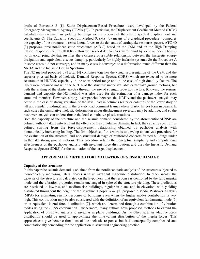
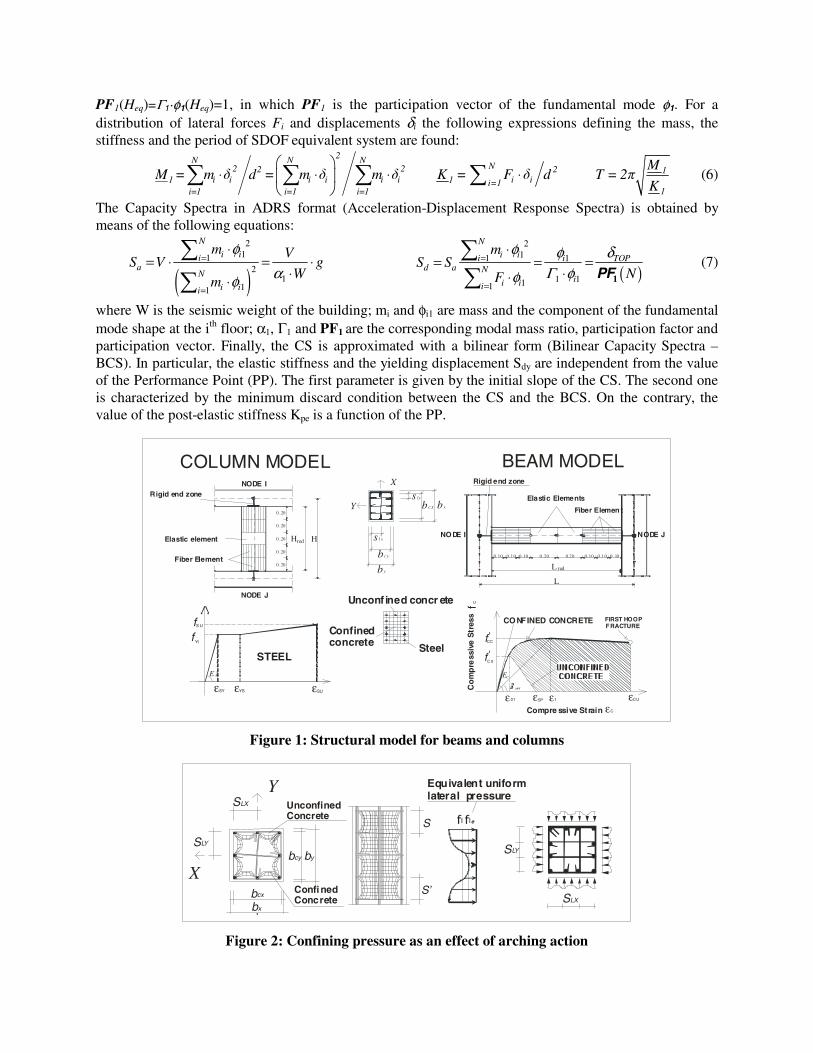
Structural model The beams and columns of the framed building were modeled with rigid end zones at the connection joints, elastic and fiber plastic elements (fig.1). Each fiber was modeled with the nonlinear stress-strain relationship of the material it was made. In particular, the cross section is composed of fibers of three different material types: confined concrete for the core, unconfined concrete for the cover, and steel for the longitudinal bars. Steel was modeled with an elastic-plastic-hardening relationship. The confined concrete was modeled with stress-strain relationships incorporating the relevant parameters of confinement (section geometry, concrete strength, type and arrangement of transverse reinforcement, its volumetric ratio, spacing and yield strength) [8,9]. The strength ccf ′ of the confine concrete was estimated with the following approximate relationships (fig.2):

cc co 1 lef = f + K f′ ′ ⋅ ( )-0.171 leK =6.7 f⋅ le,x c,x le,y c,y

lec,x c,y

f b + f bf =

b +b

⋅ ⋅ (1)

where cof ′ is the strength of unconfined concrete, lef is the equivalent uniform lateral pressure,

2le,x x l,xf K f= ⋅ and 2le,y y l,yf K f= ⋅ are the two equivalent lateral pressure acting perpendicular to core

dimensions bcx and bcy, respectively. The coefficients K2x and K2y reflect the efficiency of reinforcement arrangement. In fact, the effectiveness of lateral pressure decreases in the transverse direction as an effect of the spacing between ties, and in the longitudinal direction as an effect of the spacing between hoop bars. As an alternative to relationships based on the definition of a reduced effective area of the concrete core, the following expressions derived from the statistical analysis of tests data were applied:

2cx

2xLx l,x

bK =0.26

s s f⋅

⋅ ⋅

2cy

2yLy l,y

bK =0.26

s s f⋅

⋅ ⋅ (2)

The stress-strain relationship proposed by Popovics [10] was adopted. The tangent modulus Ec was

calculated with the formula ( )c co secE = 3320 f +6900 > E MPa suggested by Carrasquillo et. al.[11].

The strain ε1 at the maximum confined concrete stress is estimated as a function of the strain ε01 at the unconfined concrete strength, as follows:

( )1 01 1 5 3K Kε ε= ⋅ + ⋅ ⋅ 01 0.0028 0.0008 3Kε = − ⋅ 1 le coK = K f f ′⋅ ( )3co

40K = MPa

f ′ (3)

The slope of the descending branch of the stress-strain relationship is defined by the strain ε85 corresponding to 85 per cent of peak stress:

( )85 085 3 s 1 2 4ε = ε +260 K ρ ε 1+0.5 K K -1⎡ ⎤⋅ ⋅ ⋅ ⋅ ⋅⎣ ⎦ 2

085 01 3ε = ε +0.0018 K⋅ (4)

where sρ is the volumetric percentage of transverse reinforcement, and 4 ytK = f 500 .

Finally, the ultimate compressive strain εcu of confined concrete is calculated with the following parametric expression in which εsu is the ultimate tensile strain of steel:

cu s yt su ccε =0.004+1.4 ρ f ε f ′⋅ ⋅ ⋅ (5)

Equivalent Bilinear Capacity Spectrum The static nonlinear pushover analysis of the framed building gives the Capacity Curve (CC) of the structure in terms of base shear V and roof displacement δTOP. Such curve is transformed to the space of spectral displacement Sd and spectral pseudo-acceleration Sa (Capacity Spectra - CS). At this aim the MDOF 3D model is converted in a SDOF system with equivalent mass and stiffness. The displacement d of this system is equal to the lateral displacement of the structure at the height Heq where

PF1(Heq)=Γ1·φ1(Heq)=1, in which PF1 is the participation vector of the fundamental mode φ1. For a distribution of lateral forces Fi and displacements δi the following expressions defining the mass, the stiffness and the period of SDOF equivalent system are found:

2N N N2 22

i i i i i i1i=1 i=1 i=1

M = m δ d = m δ m δ⎛ ⎞

⋅ ⋅ ⋅⎜ ⎟⎝ ⎠

∑ ∑ ∑ N 2

i i1 i=1K = F δ d⋅∑ 1

1

MT = 2π

K (6)

The Capacity Spectra in ADRS format (Acceleration-Displacement Response Spectra) is obtained by means of the following equations:

( )2

112

111

N

i iia

N

i ii

m VS V g

Wm

φαφ

=

=

⋅= ⋅ = ⋅

⋅⋅

∑

∑ ( )

211 1

1 111

N

i ii i TOPd a N

ii ii

mS S

NF

φ φ δΓ φφ

=

=

⋅= = =

⋅⋅

∑

∑ 1PF (7)

where W is the seismic weight of the building; mi and φi1 are mass and the component of the fundamental mode shape at the ith floor; α1, Γ1 and PF1 are the corresponding modal mass ratio, participation factor and participation vector. Finally, the CS is approximated with a bilinear form (Bilinear Capacity Spectra – BCS). In particular, the elastic stiffness and the yielding displacement Sdy are independent from the value of the Performance Point (PP). The first parameter is given by the initial slope of the CS. The second one is characterized by the minimum discard condition between the CS and the BCS. On the contrary, the value of the post-elastic stiffness Kpe is a function of the PP.

by

bcy

s l x

bcxYs ly

bx

X

Unconf ined concr ete

Confinedconcrete Steel

εεE s

ε

STEEL

ffS U

Yt

SUYSSY

εεε

Ec

ε

'f

'f

CO NFINED CONCRETE FIRST HOOP F RACTURE

Compre ssive Strain ε

CC

C 0

C

1 CU01

Co

mp

ress

ive

Str

ess

f C

SP

0.10 0.10 0 .10 0.1 00.100.200.20 0 .10

L

L

Rigid end zone

Elastic Elements

Fiber Elemen t

NODE I NODE J

BEAM MODEL

0 .20

H H

0 .20

0 .20

0 .20

0 .20

Rigid end zone

Elastic element

Fiber Element

NODE J

COLUMN MODEL

red

red

NODE I

Figure 1: Structural model for beams and columns

X

UnconfinedConcrete

ConfinedConcrete

SLY

fl fl

SLX

e

SLY

Y

bcx

SLX

bcy by

bx

Equivalent uniformlateral pressure

S

S’

Figure 2: Confining pressure as an effect of arching action

Inelastic Seismic Demand The seismic demand is generally represented by means of the Inelastic Demand Response Spectra (IDRS). In this paper the IDRS are not directly obtained through the nonlinear time-history analysis of the equivalent bilinear SDOF system, but they are indirectly computed scaling the Elastic Demand Response Spectra (EDRS). Such scaling may be realized with two alternative approaches. The first one is based on the definition of High Damping Elastic Response Spectra (HDERS) by means of the equivalence between the viscous damping energy dissipation and the hysteretic energy dissipation. In the second approach the IDRS is obtained by scaling the EDRS (with viscous damping ratio ξ=5 per cent) by means a ductility reduction factor Rµ. In particular, the inelastic pseudo-acceleration Sa and displacement Sd - which represents the coordinates of the IDRS in ADRS format - are characterized from the coordinates [Sde;Sae] of the EDRS (ξ=5 per cent) as follows:

aea

SS

Rµ= de

dS

SRµ

µ ⋅= 2

24ae

deS T

Sπ⋅=

2

24a

dS T

Sµ

π⋅ ⋅= (8)

A great number of reduction rules are available in literature. Usually the reduction factor Rµ is an explicit function both of structural period and of characteristic periods of the earthquake. In this paper a reduction factor depending only on velocity and displacement elastic spectra was adopted. Starting from the reduction rule proposed by Ordaz et al.[12] the following expression of the strength reduction factor was proposed:

( ) ( )( ) ( )

1 v dS T S TR

PGV PGD

α µ β µ

µ⎛ ⎞ ⎛ ⎞= + ⎜ ⎟ ⎜ ⎟⎝ ⎠ ⎝ ⎠

(9)

where PGV is the peak ground velocity; PGD is the peak ground displacement; Sd(T) is the elastic spectral displacement; Sv(T) is the elastic spectral velocity; α(µ) and β(µ) are functions which have to be obtained with a statistical data analysis. In particular, for each ductility factor µ, the values of α and β were found that minimized the root-mean-square logarithmic error σ, defined as:

( )( )

2

2*

1 1

1 1ln

N Mij i

ij ii j

R T

N M R Tσ

= =

⎡ ⎤⎛ ⎞⎢ ⎥⎜ ⎟= ⋅ ⋅

⎜ ⎟⎢ ⎥⎝ ⎠⎣ ⎦∑∑ (10)

where N is the number of recordings and M is the number of structural periods considered in the analysis. For each ductility factor µ and for each period Tj the “real” reduction factor Rij is defined from the EDRS(Tj) and the IDRS(Tj,µ) of the recording i. It can be observed that the IDRS are not very sensitive to moderate variation of the strain-hardening ratio. As a consequence, they are obtained with a simple elastoplastic modelling of the SDOF equivalent system. The computed reduction factor R*

ij is obtained applying eq.9 for recording i and structural period Tj. The analysis was carried out on a group of 30 historical registrations from the European earthquake database. The seismic inputs were chosen to be consistent to Eurocode 8 type 1 elastic response spectrum for firm soil (class A). The selection was carried out minimizing the mean square error of the spectral acceleration response. In Table 1 the parameters of the earthquake registrations are reported. In particular, tREG represents the registration length, TP is the total power defined from the amplitude Fourier spectrum. Periods ranging in [0.01s; 2s] with step 0.01s and ductility factors µ=2,3,4,5,6,7,8 were considered in the analysis. In Table 2 the values of α and β minimizing the error function σ are shown. A regression model was used to characterize the variation of these parameters with the displacement ductility factor µ (Fig.3). A good fitting with very high values of the correlation parameter R is given by the following functions:

( ) ( )0.1967 log 0.454α µ µ= − ⋅ + ( ) ( )0.2314 log 0.0071β µ µ= ⋅ − (11)

Table 1. Parameters of the earthquake ground motions

Input Data Time Direction PGA /g tREG TP/PGA

2

Bevagna 26/09/97 0.33.16 NS 0.0342 46.11 5.942 Bevagna 26/09/97 9.40.30 NS 0.0756 50.31 4.350 Bevagna 26/09/97 9.40.30 EW 0.0787 50.31 5.836 Bevagna Valnerina 19/09/79 21.35.37 NS 0.0393 23.81 1.796 Bevagna Valnerina 19/09/79 21.35.37 EW 0.0235 23.81 3.878 Bolu-Bayindirlik 12/11/99 16.57.20 NS 0.7455 55.87 1.070 Bolu-Bayindirlik 12/11/99 16.57.20 EW 0.8005 55.87 0.590 Codroipo 06/05/76 20.00.13 EW 0.0877 41.32 3.176 Colfiorito 03/09/97 22.07.29 NS 0.1240 12.80 1.047 Colfiorito 03/09/97 22.07.29 EW 0.0636 12.80 0.968 Colfiorito 26/09/97 9.40.30 NS 0.1781 48.32 2.683 Colfiorito 26/09/97 9.40.30 EW 0.3298 48.32 1.064 Gebze-Tubitak 17/08/99 0.01.40 NS 0.2380 47.63 1.566 Gebze-Tubitak 17/08/99 0.01.40 EW 0.1355 47.63 2.796 Gubbio Piana 26/09/97 9.40.30 NS 0.0986 106.03 3.594 Kalamata Ote Building 13/09/86 17.24.31 NS 0.2400 29.86 1.554 Kalamata Ote Building 13/09/86 17.24.31 EW 0.2723 29.86 1.683 Lefkada Hospital 17/01/83 12.41.30 NS 0.0654 37.98 3.349 Mercato San Severino 23/11/80 18.34.52 NS 0.1079 72.31 4.535 Mercato San Severino 23/11/80 18.34.52 EW 0.1389 72.31 5.957 Petrovac Hotel Oliva 15/04/79 6.19.41 NS 0.4541 48.22 4.121 Petrovac Hotel Oliva 15/04/79 6.19.41 EW 0.3059 48.22 3.875 Rionero in Vulture 23/11/80 18.34.52 EW 0.0994 83.94 8.584 Sakarya-Bayindirlik 12/11/99 16.57.20 NS 0.0154 117.12 4.816 Sakarya-Bayindirlik 12/11/99 16.57.20 EW 0.0231 117.12 4.743 Sturno 23/11/80 18.34.52 EW 0.3229 71.93 2.202 Thessaloniky City 20/06/78 20.03.21 NS 0.1392 30.59 1.583 Tolmezzo Diga 06/05/76 20.00.13 NS 0.3568 36.53 1.004 Tolmezzo Diga 06/05/76 20.00.13 EW 0.3158 36.41 1.924 Simulated 1 (SIM 1) - - - 0.5000 40.00 11.10 Simulated 2 (SIM 2) - - - 0.5000 35.00 9.140

Table 2. Values of α and β minimizing the error σ

µ = 2 µ = 3 µ = 4 µ = 5 µ = 6 µ = 7 µ = 8 α 0.3168 0.2407 0.1840 0.1300 0.1012 0.0707 0.0481 β 0.1472 0.2507 0.3212 0.3649 0.4974 0.4430 0.4698 σ 0.0456 0.0694 0.0742 0.0883 0.1041 0.1158 0.1258

y = - 0.1967 log(µ ) + 0.454R2 = 0.9986

0

0.1

0.2

0.3

0.4

0.5

0 1 2 3 4 5 6 7 8 9µ

α

y = 0.2314Ln(x) - 0.0071R2 = 0.9984

0

0.1

0.2

0.3

0.4

0.5

0 1 2 3 4 5 6 7 8 9µ

β

Figure 3. Variation of α and β with the ductility factor µ

Improved Capacity Spectrum Method (ICSM) The calculation of the PP is realized with an iterative graphic procedure which uses the Capacity Spectrum Method based on inelastic demand Spectra. The procedure starts with the comparison between the BCS and the EDRS with damping ratio ξ=5 per cent. The intersection of the radial line corresponding to the elastic stiffness of the equivalent bilinear system and the EDRS defines the strength required for elastic behaviour of the structure. If the EDRS intersects the BCS over the yielding point this means that the structure behaves inelastically under the earthquake ground motion. In this case, eq.(8) gives the coordinates [Sa;Sd] of the IDRS from the coordinates [Sde;Sae] of the EDRS. The reduction factor Rµ is a function of the displacement ductility factor µ, and so the IDRS depends on the performance point PP which is unknown. Furthermore, the CS is modelled with a bilinear representation, and so the post-elastic acceleration Sa is greater than the yielding acceleration Say, and it depends from the PP. As a consequence, an iterative procedure has to be applied to estimate the intersection between the IDRS and the BCS. In particular, this sequence of steps has to be performed:

1) Run the pushover analysis of the building; 2) Plot the CC of the structure in terms of base shear V and roof displacement δTOP; 3) Characterize the equivalent SDOF system and plot the CS in ADRS format; 4) Define the BCS corresponding to the maximum displacement of the pushover analysis; 5) Plot the EDRS (with ξ=5 per cent); 6) Intersect the radial line corresponding to the elastic stiffness and the EDRS to obtain the

deformation demand Sd(i) and the displacement ductility demand µ(i)= Sd

(i)/ Sdy; 7) Compute the post-elastic stiffness Kpe

(i) of the BCS(i); 8) Compute the reduction factor Rµ

(i) from eq.9; 9) Plot the IDRS(i) using eq.8; 10) Intersect the IDRS(i) and the BCS(i) to estimate the new deformation demand Sd

(j) and the displacement ductility demand µ(j)= Sd

(j)/ Sdy; 11) Check for convergence. If |Sd

(i)- Sd(j)|/ Sd

(j)<tolerance (=0.05) then the earthquake deformation demand (target displacement) is Sd= Sd

(j). Otherwise repeat steps 4-10 with Sd(i)= Sd

(j); 12) Starting from the displacement Sd=d of the SDOF equivalent system, compute the lateral

displacement vector of the building given by: dd ⋅=⋅⋅= 1PF11 φδ Γ . Estimation of seismic damage The seismic demand is usually represented by inelastic strength and displacement spectra, and not in terms of hysteretic energy spectra. Furthermore, the nonlinear static procedures usually gives an estimation of the earthquake-induced deformation, while neglect the effects of cumulative damage and hysteretic energy dissipation. However, the deformation alone may be not sufficient for the evaluation of the cumulative damage, which is considered to be especially important for existing structures which have frequently not to be detailed for sustained resistance through many cycles of response into the inelastic range. In order to be used for earthquake-resistant design of the structures both at the serviceability limit state and at the failure limit state an equivalent NSP should estimate not only the lateral displacements but also the structural damage. In this paper an analysis procedure for the estimation of the structural and non-structural damage starting from the results of the ICSM is proposed. The non-structural damage is evaluated with two indices available in literature [13-14]. In particular, the damage index DI,i in walls, partitions, floors and fixtures of the ith floor is computed as a function of the interstorey drift ratio ∆i/hi, as follows:

i,

10

500I ii

D forh

∆= ≤ i i,

i i

5 1 1 1

4 500 500 100I iD forh h

⎛ ⎞∆ ∆= ⋅ − ≤ ≤⎜ ⎟⎝ ⎠

i,

i

11

100I iD forh

∆= ≥ (12)

The damage index DT,i in fittings and apparatuses is calculated as a function of the lateral displacements δi and the height H of the building, as follows:

,7

05000

iT iD for

H

δ= ≤ ,5000 7 7 1

13 5000 5000 250i i

T iD forH H

δ δ⎛ ⎞= ⋅ − ≤ ≤⎜ ⎟⎝ ⎠

,1

1250

iT iD for

H

δ= ≤ (13)

The global damage indices DI and DT, are estimated applying a weighting factor ηi which reflects the importance of elements with a higher damage index, as follows:

1

N

I i I ,ii

D D=

= η ⋅∑ 1

N

T i T ,ii

D D=

= η ⋅∑ where 1

N

i i ii

D Dη=

= ∑ (14)

The global damage index DNS in non-structural elements is given by:

NS I I T TD r D r D= ⋅ + ⋅ (15) where rI=0.75 and rT=0.25 are weighting factors which reflects the relative importance of DI and DT in the overall non-structural damage. The damage in the structural members is computed using as damage parameters the curvatures θi

+ for positive bending moment and θi

- for negative bending moment. In this paper the Park & Ang damage model [15] is modified to use the displacement ductility factor demand and the hysteretic energy ductility factor demand both for positive bending moment (µs

+, µe+) and negative (µs

-, µe-) bending moment. In this

way for the ith fiber plastic element two local damage indices are defined:

( )1 11

( / )( / ) ( / )( / ) ( / ) ( / ) ( / )i

PA,i s ,i i s ,i i e ,i( / ) ( / ) ( / ) ( / )y ,i y ,iu mon,i u mon,i

D dEM

θβµ µ β µµ θ µ

+ −+ − + −+ − + − + − + −

+ − + − + − + −

⎛ ⎞⎡ ⎤= + = + −⎜ ⎟⎣ ⎦⎜ ⎟

⎝ ⎠∫ (16)

where µs,i and µu mon,i are, respectively, the ductility factor demand and ductility factor capacity; My,i

+ e My,i

- are the yielding bending moments; dEiθ+ and dEi

θ- are the incremental values of the hysteretic energy; βi

+ and βi- are parameters accounting for the effect of cyclic loading on structural damage. These

parameters are characterized with an extension of the Park & Ang relationship obtained from the minimum variance condition between experimental and theoretical values:

( )0 447 0 073 0 24 0 314 0 7 ( / )( / ) ( / ) ( / ) ( / ) s ,ii i i i cc,i ii

. . l d . . . dE dEρ θβ ν ρ + −+ − + − + − + − += − + ⋅ + ⋅ + ⋅ ⋅ ∫ ∫ (17) where ρcc,i is the longitudinal steel ratio, ρs,i is the confinement ratio, li/di and νi are the shear span ratio and the normalised axial stress. In the case of symmetric steel areas under cyclic monotonic loading DPA,i

+=DPA,i- =DPA. In the other cases DPA,i=max(DPA,i

+;DPA,i-). The locale damage indices DPA,i are

combined in a weighted mean to give the following global damage index:

( )1

Np

PA i i PA ,ii

D w Dη=

= ⋅ ⋅∑ (18)

where the weighting factor ηi depend on the magnitude of the damage index for each fiber element, while wi is a weight which reflect the importance of the structural member in maintaining the integrity of the structure. Such weight is assumed to be linear decreasing with the height and ranging in [0.5;1]. These hypotheses lead to the following expressions:

( )

1

1

Np

i PA, jji Np

PA,k kk

r Dw

D r

=

=

⋅=

⋅

∑

∑ where

11- -1

10i

i

hr =

h

⎡ ⎤⎛ ⎞⋅⎢ ⎥⎜ ⎟⎝ ⎠⎣ ⎦

(19)

where hi is the height of structural member relative to the ground. The use of the curvatures deriving from the pushover analysis to evaluate the damage index may be not conservative. In fact, cumulative damage due to the hysteretic dissipation would be neglected. In this paper an approximate method to estimate the

structural damage is proposed. The hysteretic energy ductility factor µe,i is defined beginning from the displacement ductility factor µs,i

as follows:

2 21e,i s ,i corr ,iµ µ γ= + ⋅ with 2

1

SDMPcorr ,i i

SPSP

EE

EEγ γ

Γ= ⋅ ⋅

⋅ and i

s i

1 h,i

, y,i y,i

E

Mγ

µ θ=

⋅ (20)

In eq.20 γi is a normalised hysteretic energy parameter; EMP is the energy dissipation of the MDOF system under pushover loading up to the target displacement at the height Heq; ESP is the energy dissipation of the SDOF system corresponding to the PP; ESD represents the hysteretic energy dissipation of the SDOF system (with ξ=5 per cent) valued through the nonlinear response history analysis under the earthquake ground motion. In eq.20 the normalized hysteretic factor γi is corrected through two coefficients. The first one accounts for the relationship between plastic energy dissipated from the MDOF system and the energy dissipated from the equivalent SDOF system during the pushover analysis. The second accounts for the relationship between the hysteretic energy dissipation under seismic loading and the monotonic energy dissipation of the equivalent SDOF system. The seismic damage is finally estimated using eq.16 which combines the displacement ductility factor µs,i deriving from the pushover analysis and the equivalent hysteretic energy ductility factor µe,i given by eq.20. The degradation parameter βi defined by eq.17 accounts for the bending moment diagram and the effects of the variation of axial load in columns. The method is based on this sequence of steps:

1) Compute the performance point with the improved Capacity Spectrum Method (ICSM); 2) Run the nonlinear pushover analysis until the target displacement at the height Heq is attained; 3) Calculate the displacement ductility factors µs,i

+ and µs,i

- for each fiber element; 4) Compute the normalised hysteretic energy factor γi ; 5) Run the nonlinear dynamic analysis of the equivalent bilinear system and calculate the energy

dissipation ESD; 6) Calculate the normalised hysteretic energy factor γcorr,i and the hysteretic energy ductility factors

µe,i+

and µe,i- with eq.20;

7) Compute the degradation parameter βi from eq.17 for each fiber plastic element; 8) Calculate the local damage index from eq.16 and the global damage index from eq.18.

COMPARATIVE EVALUATION

Comparative evaluation of the ductility reduction factor In this paper the ductility reduction factor was obtained with eq.9, and so it depends on the velocity and displacement elastic spectra. The results obtained were compared with other reduction rules proposed in literature which generally requires the estimation of the characteristic periods of the earthquake. In particular, the first and widely used reduction rule was proposed by Newmark and Hall [16] and is based on energy equivalence in low period range and on displacement equivalence in medium-high period. Riddel et al.[17] presented an expression calibrated on systems with elastoplastic behaviour subjected to four different groups of seismic events. Nassar et al.[18] calibrated the reduction rule on degrading stiffness bilinear systems, and showed that the Rµ factor is independent from epicentral distance, and slightly sensitive to the type of hysteretic model. Miranda [19] formulated a reduction rule dependent on the site condition and based on bilinear systems analysis (strain-hardening ratio α=3 per cent and ductility µ ≤ 6). Vidic et al. [20] proposed an expression for reduction factor based on ‘equal displacement rule’ in medium-high period range and derived from statistical study on stiffness-degrading bilinear hysteretic systems with 10 per cent strain hardening and 5 per cent mass proportional damping. Cosenza et al. [21] proposed an expression of Rµ independent by soil characteristics and based on statistical studies of seismic Italian events. Ordaz et al.[12] carried a statistical study on a sample of 445 earthquake ground motions providing the following expression:

( ) ( )1 ( )DR S T PGDβ µ

µ = + with ( )0.173( ) 0.388 1= −β µ µ (21)

In Table 3 the comparison of the different reduction rules is shown. The comparative evaluation is carried out in terms of square-mean-root of logarithmic error σ. As shown, for each ductility value the proposed reduction rule provides the minimum error.

Table 3. Square-mean-root logarithmic error σ for different reduction rules

Reduction Rule µ = 2 µ = 3 µ = 4 µ = 5 µ = 6 µ = 7 µ = 8 Newmark-Hall 0.0683 0.1035 0.1128 0.1268 0.1464 0.1607 0.1726 Riddel-Hidalgo-Cruz 0.0716 0.1102 0.1234 0.1416 0.1665 0.1858 0.2029 Krawinkler-Nassar 0.0680 0.1033 0.1248 0.2026 0.2347 0.2618 0.2863 Miranda 0.0660 0.0978 0.1064 0.1229 0.1464 0.1660 0.1826 Vidic-Fajfar-Fischinger 0.0630 0.0994 0.1117 0.1297 0.1534 0.1761 0.2172 Cosenza-Manfredi 0.0713 0.1041 0.1132 0.1312 0.1431 0.1698 0.1837 Ordaz-Pèrez Rocha 0.0589 0.0776 0.0781 0.0911 0.1083 0.1216 0.1349 Proposed Reduction Rule 0.0456 0.0693 0.0742 0.0883 0.1041 0.1158 0.1258

Description and modelling of the buildings In order to evaluate the possibility to use the approximate method to give an estimation of the structural and non-structural damage indices two 6-storey RC framed buildings are considered (fig.4). Each building is regular in plan and in elevation and it was designed and detailed in accordance with Eurocodes 8 [1] for the High Ductility Class and the design ground acceleration 0.35 g. It is assumed that: a) the interstorey height is h=3.0m; b) at each storey all the columns have the same cross-section bCxhC; c) all the beams have the same cross-section bBxhB; d) bC=bB =b; e) the columns are tapered every two plans with taper ratio r=∆hC/hC=0.10; f) the beam span is LB=5.0 m. In such hypothesis the geometric characteristics of the building can be related to three independent parameters: 1) the fundamental period T1; 2) the ratio ρT=TX/TY between the first period in the X direction and the first period in the Y direction, this parameters is a function of the ratio βC=ICY/ICX between the moments of inertia of the column; 3) the parameter ρ=max(ρX;ρY), where ρX=ICX/IB and ρY=ICY/IB are the moment of inertia ratios between columns and beams. In particular, the fundamental period T1 may be written as follows:

3B

1 3 21 B

12 L2π 1T =

Ω E α b

⋅ ⋅⋅

(22)

where αB=hB/bB and Ω1 is the fundamental circular frequency of a structure with the same mass and the

stiffness divided for 3/B BEI L .

21

500

500

500

500500500

3

500

4 5

XY

7

6

8

9

B UIL DING R b B x hB Y

X

B UIL DING Q

500

500

500

500 500 500

21 3 4

5

6

7

8

b Bx hB C

C

Figure 4: Plan of the buildings

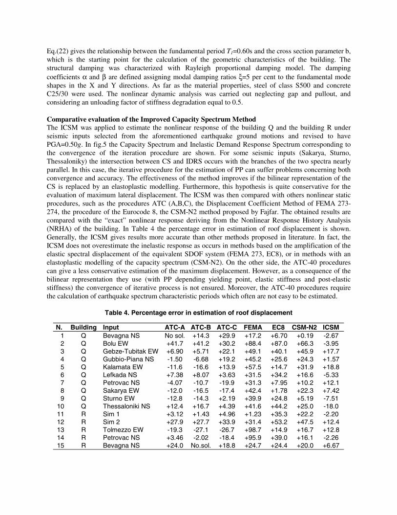
Eq.(22) gives the relationship between the fundamental period T1=0.60s and the cross section parameter b, which is the starting point for the calculation of the geometric characteristics of the building. The structural damping was characterized with Rayleigh proportional damping model. The damping coefficients α and β are defined assigning modal damping ratios ξ=5 per cent to the fundamental mode shapes in the X and Y directions. As far as the material properties, steel of class S500 and concrete C25/30 were used. The nonlinear dynamic analysis was carried out neglecting gap and pullout, and considering an unloading factor of stiffness degradation equal to 0.5. Comparative evaluation of the Improved Capacity Spectrum Method The ICSM was applied to estimate the nonlinear response of the building Q and the building R under seismic inputs selected from the aforementioned earthquake ground motions and revised to have PGA=0.50g. In fig.5 the Capacity Spectrum and Inelastic Demand Response Spectrum corresponding to the convergence of the iteration procedure are shown. For some seismic inputs (Sakarya, Sturno, Thessaloniky) the intersection between CS and IDRS occurs with the branches of the two spectra nearly parallel. In this case, the iterative procedure for the estimation of PP can suffer problems concerning both convergence and accuracy. The effectiveness of the method improves if the bilinear representation of the CS is replaced by an elastoplastic modelling. Furthermore, this hypothesis is quite conservative for the evaluation of maximum lateral displacement. The ICSM was then compared with others nonlinear static procedures, such as the procedures ATC (A,B,C), the Displacement Coefficient Method of FEMA 273-274, the procedure of the Eurocode 8, the CSM-N2 method proposed by Fajfar. The obtained results are compared with the “exact” nonlinear response deriving from the Nonlinear Response History Analysis (NRHA) of the building. In Table 4 the percentage error in estimation of roof displacement is shown. Generally, the ICSM gives results more accurate than other methods proposed in literature. In fact, the ICSM does not overestimate the inelastic response as occurs in methods based on the amplification of the elastic spectral displacement of the equivalent SDOF system (FEMA 273, EC8), or in methods with an elastoplastic modelling of the capacity spectrum (CSM-N2). On the other side, the ATC-40 procedures can give a less conservative estimation of the maximum displacement. However, as a consequence of the bilinear representation they use (with PP depending yielding point, elastic stiffness and post-elastic stiffness) the convergence of iterative process is not ensured. Moreover, the ATC-40 procedures require the calculation of earthquake spectrum characteristic periods which often are not easy to be estimated.

Table 4. Percentage error in estimation of roof displacement

N. Building Input ATC-A ATC-B ATC-C FEMA EC8 CSM-N2 ICSM 1 Q Bevagna NS No sol. +14.3 +29.9 +17.2 +6.70 +0.19 -2.67 2 Q Bolu EW +41.7 +41.2 +30.2 +88.4 +87.0 +66.3 -3.95 3 Q Gebze-Tubitak EW +6.90 +5.71 +22.1 +49.1 +40.1 +45.9 +17.7 4 Q Gubbio-Piana NS -1.50 -6.68 +19.2 +45.2 +25.6 +24.3 +1.57 5 Q Kalamata EW -11.6 -16.6 +13.9 +57.5 +14.7 +31.9 +18.8 6 Q Lefkada NS +7.38 +8.07 +3.63 +31.5 +34.2 +16.6 -5.33 7 Q Petrovac NS -4.07 -10.7 -19.9 +31.3 +7.95 +10.2 +12.1 8 Q Sakarya EW -12.0 -16.5 -17.4 +42.4 +1.78 +22.3 +7.42 9 Q Sturno EW -12.8 -14.3 +2.19 +39.9 +24.8 +5.19 -7.51

10 Q Thessaloniki NS +12.4 +16.7 +4.39 +41.6 +44.2 +25.0 -18.0 11 R Sim 1 +3.12 +1.43 +4.96 +1.23 +35.3 +22.2 -2.20 12 R Sim 2 +27.9 +27.7 +33.9 +31.4 +53.2 +47.5 +12.4 13 R Tolmezzo EW -19.3 -27.1 -26.7 +98.7 +14.9 +16.7 +12.8 14 R Petrovac NS +3.46 -2.02 -18.4 +95.9 +39.0 +16.1 -2.26 15 R Bevagna NS +24.0 No.sol. +18.8 +24.7 +24.4 +20.0 +6.67

0.0

0.5

1.0

1.5

2.0

2.5

0 5 10 15 20

Sd (cm)

Sa/g

EDRS

IDRSCS

BCS

T=0.1 T=0.4

T=0.7

T=1

BEVAGNA

PP

0.0

0.5

1.0

1.5

2.0

2.5

0 5 10 15 20

Sd (cm)

Sa/g

T=0.1 T=0.4

T=0.7

T=1

KALAMATA

PP

EDRS

IDRS

0.0

0.5

1.0

1.5

2.0

2.5

0 5 10 15 20

Sd (cm)

Sa/g

T=0.1 T=0.4

T=0.7

T=1

PETROVAC

PP

EDRS

IDRS

0.0

0.5

1.0

1.5

2.0

2.5

0 5 10 15 20

Sd (cm)

Sa/g

EDRS

IDRS

BCS

T=0.1T=0.4

T=0.7

T=1

GEBZE

PP

0.0

0.4

0.8

1.2

1.6

2.0

0 5 10 15 20

Sd (cm)

Sa/g

EDRS

IDRSBCS

T=0.1 T=0.4

T=0.7

T=1

SIM 1

PP

0.0

0.4

0.8

1.2

1.6

2.0

0 5 10 15 20

Sd (cm)

Sa/g

EDRS

IDRSCS

BCS

T=0.1 T=0.4

T=0.7

T=1

TOLMEZZO EW

PP

Figure 5. Improved Capacity Spectrum Method: Calculation of Performance Point

Comparative evaluation of the seismic damage The calculation of the lateral displacement with the ICSM is the starting point for the estimation of seismic damage both in structural members and in non-structural parts of the building. In Fig.6 the values of the non-structural damage index DNS at each floor are plotted. In particular, the comparison between the results obtained with the NRHA and the ICSM is carried out. When the estimation of the PP is accurate, the proposed method gives a good approximation of the non-structural damage.

BEVAGNA

1

2

3

4

5

6

0.2 0.4 0.6 0.8 1.0 1.2D NS

FL

OO

R

BOLU

1

2

3

4

5

6

0.2 0.4 0.6 0.8 1.0 1.2D NS

FL

OO

R

GEBZE

1

2

3

4

5

6

0.2 0.4 0.6 0.8 1.0 1.2D NS

FL

OO

R

GUBBIO

1

2

3

4

5

6

0.2 0.4 0.6 0.8 1.0 1.2D NS

FL

OO

R KALAMATA

1

2

3

4

5

6

0.2 0.4 0.6 0.8 1.0 1.2D NS

FL

OO

R

LEFKADA

1

2

3

4

5

6

0.2 0.4 0.6 0.8 1.0 1.2D NS

FL

OO

R

PETROVAC

1

2

3

4

5

6

0.2 0.4 0.6 0.8 1.0 1.2D NS

FL

OO

R SAKARYA

1

2

3

4

5

6

0.2 0.4 0.6 0.8 1.0 1.2D NS

FL

OO

R STURNO

1

2

3

4

5

6

0.2 0.4 0.6 0.8 1.0 1.2D NS

FL

OO

R THESSAL.

1

2

3

4

5

6

0.2 0.4 0.6 0.8 1.0 1.2D NS

FL

OO

R

SIM 1

1

2

3

4

5

6

0.2 0.4 0.6 0.8 1.0 1.2D NS

FL

OO

R

SIM 2

1

2

3

4

5

6

0.2 0.4 0.6 0.8 1.0 1.2D NS

FL

OO

R TOLMEZZO

1

2

3

4

5

6

0.2 0.4 0.6 0.8 1.0 1.2D NS

FL

OO

R PETROVAC

1

2

3

4

5

6

0.2 0.4 0.6 0.8 1.0 1.2D NS

FL

OO

R BEVAGNA

1

2

3

4

5

6

0.2 0.4 0.6 0.8 1.0 1.2D NS

FL

OO

R

NRHA ICSM

Figure 6: Non-structural damage index: Comparison between NRHA and ICSM

BEVAGNA

1

2

3

4

5

6

0.0 0.3 0.5 0.8 1.0D BEAM

FL

OO

R MAX

GLOBAL

BOLU

1

2

3

4

5

6

0.0 0.1 0.2 0.3 0.4D BEAM

FL

OO

R

GLOBAL

MAX

GEBZE

1

2

3

4

5

6

0.0 0.1 0.2 0.3 0.4D BEAM

FL

OO

R MAXGLOBAL

GUBBIO

1

2

3

4

5

6

0.0 0.1 0.2 0.3 0.4 0.5D BEAM

FL

OO

R MAX

GLOBAL

KALAMATA

1

2

3

4

5

6

0.0 0.2 0.3 0.5 0.6D BEAM

FL

OO

R MAX

GLOBAL

LEFKADA

1

2

3

4

5

6

0.0 0.1 0.2 0.3 0.4D BEAM

FL

OO

R MAX

GLOBAL

PETROVAC

1

2

3

4

5

6

0.0 0.2 0.4 0.6 0.8D BEAM

FL

OO

R MAX

GLOBAL

SAKARYA

1

2

3

4

5

6

0.0 0.1 0.2 0.3 0.4 0.5D BEAM

FL

OO

R

MAX

GLOBAL

STURNO

1

2

3

4

5

6

0.0 0.1 0.2 0.3 0.4 0.5D BEAM

FL

OO

R

MAX

GLOBAL

THESSALONIKI

1

2

3

4

5

6

0.0 0.2 0.4 0.6 0.8D BEAM

FL

OO

R

GLOBAL

MAX

SIM 1

1

2

3

4

5

6

0.0 0.1 0.2 0.3 0.4 0.5D BEAM

FL

OO

R

MAX

GLOBAL

SIM 2

1

2

3

4

5

6

0.0 0.1 0.2 0.3 0.4 0.5D BEAM

FL

OO

R

MAXGLOBAL

TOLMEZZO

1

2

3

4

5

6

0.0 0.1 0.2 0.3 0.4 0.5D BEAM

FL

OO

RMAX

GLOBAL

PETROVAC

1

2

3

4

5

6

0.0 0.1 0.2 0.3 0.4 0.5D BEAM

FL

OO

R

MAX

GLOBAL

BEVAGNA

1

2

3

4

5

6

0.0 0.1 0.2 0.3 0.4 0.5D BEAM

FL

OO

R

MAX

GLOBAL

NRHA ICSM

Figure 7: Seismic damage in beams: Comparison between NRHA and ICSM

BEVAGNA

1

2

3

4

5

6

0.0 0.3 0.5 0.8 1.0D COL

FL

OO

R MAX

GLOBAL

BOLU

1

2

3

4

5

6

0.0 0.1 0.2 0.3 0.4D COL

FL

OO

R

GLOBALMAX

GEBZE

1

2

3

4

5

6

0.0 0.1 0.2 0.3 0.4D COL

FL

OO

R MAXGLOBAL

GUBBIO

1

2

3

4

5

6

0.0 0.1 0.2 0.3 0.4 0.5D COL

FL

OO

R MAXGLOBAL

KALAMATA

1

2

3

4

5

6

0.0 0.2 0.4 0.6D COL

FL

OO

R

MAX

GLOBAL

LEFKADA

1

2

3

4

5

6

0.0 0.1 0.2 0.3 0.4D COL

FL

OO

R MAXGLOBAL

PETROVAC

1

2

3

4

5

6

0.0 0.2 0.4 0.6 0.8D COL

FL

OO

R MAXGLOBAL

SAKARYA

1

2

3

4

5

6

0.0 0.1 0.2 0.3 0.4 0.5D COL

FL

OO

R

MAX

GLOBAL

STURNO

1

2

3

4

5

6

0.0 0.1 0.2 0.3 0.4 0.5D COL

FL

OO

R MAXGLOBAL

THESSAL.

1

2

3

4

5

6

0.0 0.2 0.4 0.6 0.8D COL

FL

OO

R

SIM 1

1

2

3

4

5

6

0.0 0.1 0.2 0.3 0.4D COL

FL

OO

R

MAX

GLOBAL

SIM 2

1

2

3

4

5

6

0.0 0.1 0.2 0.3 0.4 0.5D COL

FL

OO

R

MAX

GLOBAL

TOLMEZZO

1

2

3

4

5

6

0.0 0.1 0.2 0.3 0.4D COL

FL

OO

R

MAX

GLOBAL

PETROVAC

1

2

3

4

5

6

0.0 0.1 0.2 0.3 0.4D COL

FL

OO

R

MAX

GLOBAL

BEVAGNA

1

2

3

4

5

6

0.0 0.1 0.2 0.3 0.4D COL

FL

OO

R

MAX

GLOBAL

NRHA ICSM

Figure 8: Seismic damage in columns: Comparison between NRHA and ICSM

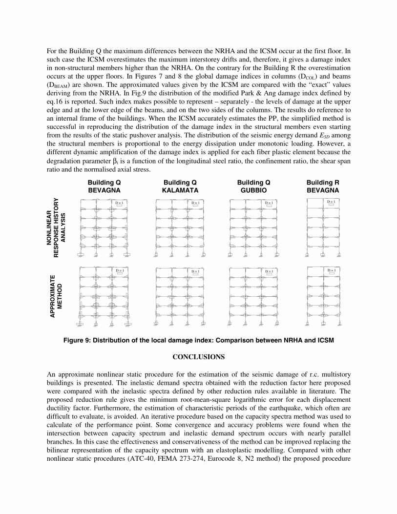
For the Building Q the maximum differences between the NRHA and the ICSM occur at the first floor. In such case the ICSM overestimates the maximum interstorey drifts and, therefore, it gives a damage index in non-structural members higher than the NRHA. On the contrary for the Building R the overestimation occurs at the upper floors. In Figures 7 and 8 the global damage indices in columns (DCOL) and beams (DBEAM) are shown. The approximated values given by the ICSM are compared with the “exact” values deriving from the NRHA. In Fig.9 the distribution of the modified Park & Ang damage index defined by eq.16 is reported. Such index makes possible to represent – separately - the levels of damage at the upper edge and at the lower edge of the beams, and on the two sides of the columns. The results do reference to an internal frame of the buildings. When the ICSM accurately estimates the PP, the simplified method is successful in reproducing the distribution of the damage index in the structural members even starting from the results of the static pushover analysis. The distribution of the seismic energy demand ESD among the structural members is proportional to the energy dissipation under monotonic loading. However, a different dynamic amplification of the damage index is applied for each fiber plastic element because the degradation parameter βi is a function of the longitudinal steel ratio, the confinement ratio, the shear span ratio and the normalised axial stress.

Building Q BEVAGNA

Building Q KALAMATA

Building Q GUBBIO

Building R BEVAGNA

NO

NL

INE

AR

R

ES

PO

NS

E H

IST

OR

Y

AN

AL

YS

IS

D = 1

D = 1

D = 1

D = 1

AP

PR

OX

IMA

TE

M

ET

HO

D

D = 1

D = 1

D = 1

D = 1

Figure 9: Distribution of the local damage index: Comparison between NRHA and ICSM

CONCLUSIONS An approximate nonlinear static procedure for the estimation of the seismic damage of r.c. multistory buildings is presented. The inelastic demand spectra obtained with the reduction factor here proposed were compared with the inelastic spectra defined by other reduction rules available in literature. The proposed reduction rule gives the minimum root-mean-square logarithmic error for each displacement ductility factor. Furthermore, the estimation of characteristic periods of the earthquake, which often are difficult to evaluate, is avoided. An iterative procedure based on the capacity spectra method was used to calculate of the performance point. Some convergence and accuracy problems were found when the intersection between capacity spectrum and inelastic demand spectrum occurs with nearly parallel branches. In this case the effectiveness and conservativeness of the method can be improved replacing the bilinear representation of the capacity spectrum with an elastoplastic modelling. Compared with other nonlinear static procedures (ATC-40, FEMA 273-274, Eurocode 8, N2 method) the proposed procedure

generally gives a more accurate estimation of the maximum lateral displacements obtained from nonlinear response history analysis of the building. An extension of the Park & Ang damage model was used to define the damage index in structural members. For each fiber plastic element the energy ductility factor was characterized starting from the rotation ductility factor deriving from the static pushover analysis. At this aim, an amplification factor defined from the static and the seismic analysis of the bilinear equivalent SDOF system and from the pushover analysis of the building was proposed. The results obtained were compared with the damage index derived from the nonlinear response history analysis of the building. In the cases studied the simplified method seemed to be successful in reproducing the distribution of the damage index in the structural members.

REFERENCES 1. Eurocode 8, “Design of structures for earthquake resistance”, Final PT Draft, prEN 1998-1, 2003. 2. FEMA, “NEHRP Guidelines for the seismic rehabilitation of buildings”. 273-274, 1997. 3. ATC, “Seismic evaluation and retrofit of concrete buildings”, Rep.ATC-40, Redwood City,3, 1996. 4. Fajfar P., “Capacity Spectrum Method based on Inelastic Demand Spectra”, Earth. Eng. and Struct.

Dyn., 28, 979-993, 1999. 5. Chopra A.K., Goel R.K. “A modal Pushover analysis procedure for estimating seismic demands for

buildings”, Earth.Eng. and Struct. Dyn., 2002, 561-582. 6. Valles R., Reinhorn A., Kunnath S. IDARC2D version 4.0: A Computer Program for the Inelastic

Analysis of Buildings”m Technical Report NCEER-96-0010, NCEER, Buffalo, NY, 1996. 7. Freeman S.A., “The Capacity Spectrum Method as a Tool for Seismic Design”, Proc. 11° European

Conference on Earthquake Engineering, Paris, 1997. 8. Mander J.B., Priestley M., Park R., “Theoretical Stress-Strain Model for Confined Concrete”,

Journal of Structural Engineering, 114, ASCE,1804-1825, 1988. 9. Razvi S., Saatcioglu M., “Confinement Model for High-Strength Concrete”, Journal of Structural

Engineering, 125, ASCE, 1999. 10. Popovics S., “Numerical Approach to the Complete Stress-Strain Relation for Concrete.”, Cement

And Concrete Res., 3(5), 583-599, 1973. 11. Carrasquillo R.L., Nilson A.H., Slate F.O., “Properties of High-Strength Concrete Subjected to

Short Term Load”, Aci J., 78(3), 171-178, 1981. 12. Ordaz M., Pèrez-Rocha L.E., “Estimation of strength-reduction factors for elastoplastic systems:

New approach”, Earthquake Engineering and Structural Dynamics, 27, 889-901, 1998. 13. Galambos T.V., Ellingwood B., “Serviceability limit states: Deflection”, Journal of Structural

Engineering, 112(1), ASCE, 67-85, 1986. 14. Savino C., Terenzi G., Vignoli A., “Analisi della risposta dinamica e valutazione del

danneggiamento di strutture isolate alla base”, Ingegneria Sismica, 2, 21-37, 1997. 15. Park Y. J., Ang A. H.S., “Mechanistic seismic damage model for reinforced concrete”, Journal of

Structural Engineering, 111(4), ASCE, 722-739, 1985. 16. Newmark N.M., Hall W.J., “Seismic design criteria for nuclear reactor facilities”, Building Practices

for Disaster Mitigation Rep. No. 46, Nat. Bureau of Stand., 209-236, 1973. 17. Riddel R., Hidalgo O.P., Cruz E.F., “Response modification factors for earthquake resistant design

of short period buildings”, Earthquake Spectra, 5(3): 571-590, 1989. 18. Nassar A.A., Krawinkler H., „Seismic demands for SDOF and MDOF systems”, Rep. No. 95, John

A. Blume Ctr., Stanford University, Cal., 1991. 19. Miranda E., “Site-dependent strength reduction factors”J.Str.Eng.,ASCE,119(12),3503-3519, 1993. 20. Vidic T., Fajfar P., Fischinger M., “Consistent inelastic design spectra: strenght and displacement”

Earth. Eng. and Struct. Dyn., 23:507-521, 1994. 21. Cosenza E., Manfredi G., “Indici e misure di danno nella progettazione sismica”, CNR-GNDT, 2000.