approach for combining fault and area sources in seismic

Nat. Hazards Earth Syst. Sci., 18, 2809–2823, 2018https://doi.org/10.5194/nhess-18-2809-2018© Author(s) 2018. This work is distributed underthe Creative Commons Attribution 4.0 License.

Approach for combining fault and area sources in seismichazard assessment: application in south-eastern SpainAlicia Rivas-Medina1,2, Belen Benito1, and Jorge Miguel Gaspar-Escribano1

1Departamento de Ingeniería Topográfica y Cartografía, Universidad Politécnica de Madrid, Madrid, Spain2Departamento de Ingeniería Civil, Universidad de Concepción, Concepción, Chile

Correspondence: Alicia Rivas-Medina ([email protected])

Received: 2 February 2018 – Discussion started: 13 March 2018Revised: 1 August 2018 – Accepted: 10 October 2018 – Published: 30 October 2018

Abstract. This paper presents a methodological approach toseismic hazard assessment based on a hybrid source modelcomposed of faults as independent entities and zones con-taining residual seismicity. The seismic potential of bothtypes of sources is derived from different data: for the zones,the recurrence model is estimated from the seismic cata-logue. For fault sources, it is inferred from slip rates derivedfrom palaeoseismicity and GNSS (Global Navigation Satel-lite System) measurements.

Distributing the seismic potential associated with eachsource is a key question when considering hybrid zone andfault models, and this is normally resolved using one of twopossible alternatives: (1) considering a characteristic earth-quake model for the fault and assigning the remaining mag-nitudes to the zone, or (2) establishing a cut-off magnitude,Mc, above which the seisms are assigned to the fault and be-low which they are considered to have occurred in the zone.This paper presents an approach to distributing seismic po-tential between zones and faults without restricting the mag-nitudes for each type of source, precluding the need to es-tablish cut-off Mc values beforehand. This is the essentialdifference between our approach and other approaches thathave been applied previously.

The proposed approach is applied in southern Spain, aregion of low-to-moderate seismicity where faults moveslowly. The results obtained are contrasted with the resultsof a seismic hazard method based exclusively on the zonemodel. Using the hybrid approach, acceleration values showa concentration of expected accelerations around fault traces,which is not appreciated in the classic approach using onlyzones.

1 Introduction

Active faults are the main earthquake sources in the crust.However, their incorporation in seismic hazard assessmentis not straightforward since there are not enough data avail-able to adequately model them. This leads to a limited use offaults as independent sources in seismic hazard analyses andto an extended use of seismic zones that cover a significantportion of the crust, assuming uniform seismic characteris-tics within each source.

This situation has begun to change in recent years, asmore studies on active tectonics, palaeoseismicity and faultdeformation rates derived from GNSS and other measure-ments become available. These recently available studiesconstrain fault parameters such as rupture plane geometry,predominant sense of slip, slip rates, etc. (e.g. Dixon et al.,2003; Langbein and Bock, 2004; Papanikolaou et al., 2005;Walpersdorf et al., 2014; Metzger et al., 2011).

Taking fault type rather than zones into consideration inseismic hazard studies requires addressing two factors: the3-D geometry of the source and the data required to charac-terize its seismic potential. In most practical cases, the seis-mic potential of faults is characterized based on the slip rateusing characteristic earthquake models proposed by Wes-nousky (1986) (for instance, Field et al., 2014; Akinci andPace, 2017) instead of Gutenberg–Richter recurrence mod-els (Parsons and Geist, 2009). Other approaches such as ex-tracting the seismic parameters of every single fault from theearthquake catalogue are not always viable, especially in ar-eas with slow-moving faults. Additionally, the period con-sidered in the catalogue may be too short compared with therecurrence time of the fault to provide an unbiased estimationof fault seismic parameters.

Published by Copernicus Publications on behalf of the European Geosciences Union.

2810 A. Rivas-Medina et al.: Approach for combining fault and area sources in seismic hazard assessment

In principle, modelling all existing active faults as inde-pendent entities could be conceived as the most accuratesource model for seismic hazard assessment. However, thisvision is still rather idealistic. A more realistic view wouldinclude only a limited number of active faults (those withthe highest seismic activity) as independent sources. Ac-cordingly, small faults that generate low-magnitude events orslow faults that produce rare events cannot be properly char-acterized. To prevent a possible deficit in the seismic sourcemodel for a given region, the use of faults as seismic sourcesmay be completed with zones that account for the seismicpotential associated with these small or slow faults or sim-ply with unknown faults that cannot be characterized inde-pendently. Hence, we propose considering a hybrid sourcemodel composed of faults and zones: the first modelled asindependent sources and the second including residual seis-micity.

Adequately establishing the distribution of seismic poten-tial using a model that combines zones and faults poses achallenge, since these are derived from different data sources.For zones, the recurrence model is calculated based on theseismic catalogue, whereas for faults, the recurrence modelis derived from fault geometries and slip rate estimates basedon GNSS-measured deformation rates. The problem is thatsome of the events contained in the catalogue may be asso-ciated with the faults and may have already been includedwhen calculating the seismic potential of the faults based onthe slip rate estimates. If all events are assigned to the zone,the events associated with the faults would be counted twice,leading to an overestimation of the total seismic potential (forboth faults and zones).

Some authors assign initial β values to seismic sources(e.g. Bungum, 2007) or propose a simple way of distributingthe seismic potential based on a uniform magnitude value,Mc, assigning events with a magnitude lower than Mc to thezone and events with magnitude higher than Mc to the faults(Frankel, 1995; Woessner et al., 2015). The question is, howis this Mc value determined? Why can the fault not generateevents with a magnitude below the Mc value? In a study re-gion such as southern Spain, with slow faults and maximummagnitudes around 6.5–7.0, it is difficult to choose an Mc ina non-arbitrary manner.

The approach presented in this paper addresses the chal-lenging question of how to estimate the anticipated groundmotion exceedance rate using a short period of earthquakeobservations and limited geological data (with significant un-certainties). This challenge is common to all probabilisticseismic hazard models (Kijko et al., 2016). The purpose ofthis study is to approach this challenge proposing a modelthat contains different types of seismic sources (faults andzones) and adequately distributes the seismic potential, pre-venting double counting and taking completeness periodsinto account.

Seismic potential

of the regionSeismic potential of

the zoneSeismic potential

of the faults

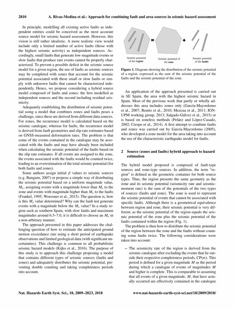
Figure 1. Diagram showing the distribution of the seismic potentialof a region, expressed as the sum of the seismic potential of thefaults and the seismic potential of the zone.

An application of the approach presented is carried outin SE Spain, the area with the highest seismic hazard inSpain. Most of the previous work that partly or wholly ad-dresses this area includes zones only (García-Mayordomoet al., 2007; Benito et al., 2010; Mezcua et al., 2011; IGN-UPM working group, 2013; Salgado-Gálvez et al., 2015) oris based on zoneless methods (Peláez and López-Casado,2002; Crespo et al., 2014). A first attempt to combine faultsand zones was carried out by García-Mayordomo (2005),who developed a zone model for the area taking into accountthe use of the characteristic earthquake model for faults.

2 Source (zones and faults) hybrid approach to hazardestimation

The hybrid model proposed is composed of fault-typesources and zone-type sources. In addition, the term “re-gion” is defined as the geometric container for both sourcetypes. Thus, the region presents the same geometry as thezone and its seismic potential (seismicity rate and seismic-moment rate) is the sum of the potentials of the two typesof sources (faults and zone). The zone is used to representthe seismic potential of events that cannot be associated withspecific faults. Although there is a geometrical equivalencebetween region and zone, their seismic potential is very dif-ferent, as the seismic potential of the region equals the seis-mic potential of the zone plus the seismic potential of thefaults contained within the region (Fig. 1).

The problem is then how to distribute the seismic potentialof the region between the zone and the faults without count-ing some faults twice. The following considerations weretaken into account:

– The seismicity rate of the region is derived from theseismic catalogue after excluding the events that lie out-side their respective completeness periods, CP(m). Thisperiod is defined for a given magnitude M as the periodduring which a catalogue of events of magnitudes Mand higher is complete. This is comparable to assumingthat all events of a given magnitude, M , that have actu-ally occurred are effectively contained in the catalogue

Nat. Hazards Earth Syst. Sci., 18, 2809–2823, 2018 www.nat-hazards-earth-syst-sci.net/18/2809/2018/

A. Rivas-Medina et al.: Approach for combining fault and area sources in seismic hazard assessment 2811

0.0

0.1

0.2

0.3

0.4

0.5

0.6

0.7

0.8

0.9

1.0

1300

1350

1400

1450

1500

1550

1600

1650

1700

1750

1800

1850

1900

1950

2000

Cum

ulat

ive

num

ber o

f ear

thqu

akes

nor

mal

ized

CP [6.0 – 6.5) ?

To

CP (4.0 - 4.5)

CP[4.5 – 5.0)

CP [5.0 – 5.5)

CP [5.5 – 6.0)

CP [6.5 < ) ?

MMin = 4.0

MMaxC = 5.9

MMax ?

AR [4.0 – 4.5)

AR [4.5 – 5.0)

AR [5.0 – 5.5)

AR [5.5 – 6.0)

Time (years)

Mag

nitu

de

OP

(a)

(b)

Figure 2. Completeness analyses of the seismic catalogue. Panel (a) shows the (normalized) cumulative number of earthquakes per yearfor different magnitude intervals. Solid circles indicate the inflection point that marks the lower limit of the completeness period for therespective magnitude interval CP(m). Panel (b) shows the CP(m) corresponding to each magnitude interval. Note that the CP(m) is not wellconstrained for magnitudes above the MMaxC value (note dashed and dotted curves in both figures).

within the period CP(m=M) (and not outside of thisperiod).

– The completeness periods, CP(m), for different magni-tudes up to a maximum-completeness magnitude value,MMaxC, are lower than the observation period (OP) ofthe catalogue.

– Magnitude values above MMaxC present recurrence pe-riods higher than the catalogue OP. These values usuallyconstitute a sample that does not include a high enoughnumber of records to clearly establish the recurrence pe-riod, as this makes it increasingly difficult to constrainrates for rarer events.

By representing the number of recorded events for differ-ent magnitude intervals as a function of time it is possibleto identify the reference years, RY(m), for different magni-tude intervals using the slope method (Hakimhashemi andGrünthal, 2012), also known as the temporal course of earth-quake frequency (TCEF) (Nasir et al., 2013). This methodconsists of plotting the cumulative number of earthquakesof a given magnitude range over time and estimating theyear, presenting a significant gradual change in slope (Fig. 2).

Consequently, CP(m) and MMaxC values can be calculatedfor m<=MMaxC. It is then possible to estimate seismicityrates (Eq. 1) and the seismic moment in each magnitude in-terval (Eq. 2) as follows:

n(m)=n(m)

CP(m), (1)

where n(m) is the annual rate of events with magnitude (m)and n(m) is the number of recorded events with magni-tude (m) in the catalogue in the completeness period, CP(m).

Mo(m)= (m) ·Mo(m), (2)

where Mo(m) is the seismic moment released by eventsof magnitude m, obtained using the equation proposed byHanks and Kanamori (1979) (log(Mo)= 1.5 ·Mw+ 16.1).

Finally, the cumulative rates in the interval [MMin,MMaxC]can be estimated, where MMin is the minimum-magnitudevalue used to compute seismic hazard, as shown in Sect. 2.1.This is illustrated with an example in Fig. 2, with [MMin,MMaxC] = [4.0, 5.9].

Although faults are capable of generating earthquakeswith magnitude m>MMaxC, the distribution of seismic po-tential is carried out in the completeness period [MMin,

www.nat-hazards-earth-syst-sci.net/18/2809/2018/ Nat. Hazards Earth Syst. Sci., 18, 2809–2823, 2018


MMaxC]. In this way, we avoid using magnitudes with longrecurrence periods that have not been recorded in the cat-alogue within the completeness periods. The computationof the seismic potential of the fault in the interval [MMaxC,MMax(fault)], where MMax(fault) is the maximum-magnitudevalue of events that can be generated in a fault, is constrainedwith other geological criteria (see below).

The seismic potential is represented by the total rate ofearthquakes (Nmin) and the cumulative rate of seismic mo-ment (Mo), for the magnitude range [MMin, MMaxC], in thecompleteness period CP(m). Details on how to determineNmin and Mo for the entire region, the corresponding zoneand faults are explained in the following section.

2.1 Seismic potential of the region

The Nmin and Mo values representing the seismic potential ofthe region are derived from the seismic catalogue of the mag-nitude interval [MMin, MMaxC] for the completeness periods,CP(m).

Nminregion

∣∣MMaxCMMin

=

MMaxC∑MMin

n(m) (3)

Moregion

∣∣MMaxCMMin

=

MMaxC∑MMin

n(m) ·Mo(m), (4)

with n(m) the annual rate of events with magnitude (m)recorded in CP(m) and Mo(m) the seismic moment for mag-nitude m. The notation X|

Mj

Mirepresents the magnitude inter-

val (Mi , Mj ) in which variable X is computed.

2.2 Seismic potential of faults

The cumulative-moment rate of the faults is estimated as-suming that the fault planes are accumulating energy evenlyand using the equation proposed by Brune (1968):

Mofault = υ ·µ ·A, (5)

where υ is the slip rate, µ is the shear modulus and A is thearea of the fault plane.

The slip rate υ and the area of each fault plane can bederived from specific studies based on paleoseismic analy-ses and GNSS measurements. There are also some databasesavailable to search for these data, including the EDSF for Eu-rope (Basili et al., 2013), the DISS for Italy (DISS WorkingGroup, 2018) and the QAFI for Spain and Portugal (Garcia-Mayordomo et al., 2012). The shear modulus may be esti-mated from values close to µ= 3.2×1010 Pa (Walters et al.,2009; Martínez-Díaz et al., 2012).

This moment rate represents the average annual seismicmoment accumulated in each fault that will be releasedby earthquakes of different magnitudes m= 0 up to themaximum magnitude of the fault, MMax(fault). The valueMMax(fault) can be evaluated from a geometrical aspect of the

fault planes using empirical relationships proposed in the lit-erature, such as Wells and Coppersmith (1994), Stirling et al.(2002) and Leonard (2010). Thus, Mofault can be expressedas follows (Eq. 6):

Mofault =

MMax(fault)∫Mm=0

n(m) ·Mo(m)dm, (6)

where n(m) can be estimated applying a recurrence model,for instance, the modified GR model shown in Eq. (7).

n(m)= Nminfault ·β

e−βm

e−β (Mm=0)− e−β

(MMax(fault)

) , (7)

and the seismic moment Mo(m), can be estimated fromthe Hanks and Kanamori (1979) relation expressed in ex-ponential terms, Mo(m)= e

dm+c with c = 16.1 · ln(10) andd = 1.5 · ln(10), wherem is the moment magnitudeMw (An-derson and Luco, 1983).

Substituting the previous relations in Eq. (6), solving theintegral and reordering the equation for Nminfault , we getEq. (9).

Nminfault =

Mofault · (dβ) ·

(e−β(Mm=0)− e

−β(MMax(fault)

))β ·[e−βMMaxMo(MMax(fault))− e−βMm=0Mo(Mm=0)

] ,(8)

where Mm=0 is the minimum magnitude that may be gener-ated at a fault rupture (here taken as m= 0), MMax(fault) themaximum magnitude, and Mofault the seismic-moment rateaccumulated in the fault (Eq. 5).

The total seismic-moment rate for each fault (Mofault) andseismicity rate (Nminfault ) can be formulated as the sum of theseismic-moment rate released at different magnitude inter-vals; thus, it follows

Nminfault = Nmin∣∣MMinMM=0

+ Nmin∣∣MMaxCMMin

+ Nmin∣∣MMax(fault)MMaxC

(9)

Mofault =

MMin∑MM=0

n(m) ·Mo(m)+

MMaxC∑MMin

n(m) ·Mo(m)

+

MMax(fault)∑MMaxC

n(m) ·Mo(m). (10)

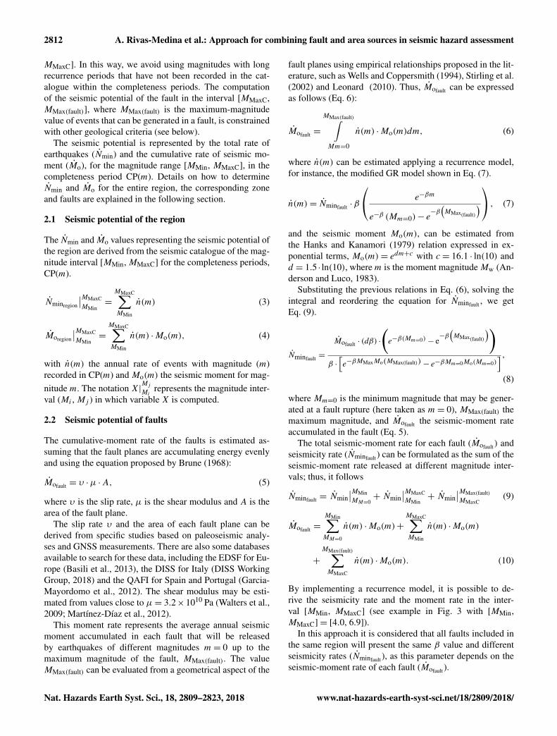
By implementing a recurrence model, it is possible to de-rive the seismicity rate and the moment rate in the inter-val [MMin, MMaxC] (see example in Fig. 3 with [MMin,MMaxC] = [4.0, 6.9]).

In this approach it is considered that all faults included inthe same region will present the same β value and differentseismicity rates (Nminfault ), as this parameter depends on theseismic-moment rate of each fault (Mofault ).



Figure 3. (a) Seismicity rate (cumulative number of events per year vs. magnitude) and (b) moment rate (cumulative seismic moment peryear vs. magnitude) plots. The different magnitude intervals mentioned in the text are marked.

2.3 Seismic potential of the zone

The parameters representing the zone are initially unknown.They can be calculated for the interval [MMin, MMaxC] giventhat

Seismic Potentialzone = Seismic Potentialregion

−Seismic Potentialfaults, (11)

or specifically,

Nminzone

∣∣MMaxCMMin

= Nminregion

∣∣MMaxCMMin

−

∑Nminfault

∣∣MMaxCMMin

(12)

Mozone

∣∣MMaxCMMin

= Moregion

∣∣MMaxCMMin

−

∑Mofault

∣∣MMaxCMMin

. (13)

In principle, there are two equations with two unknowns re-lated to the zone:

Nminzone

∣∣MMaxCMMin

,

and

Mozone

∣∣MMaxCMMin

.

Regarding the faults, Nminfault |MMaxCMMin

and Mofault |MMaxCMMin

arederived using an initial (not definitive) β value. Regardingthe region, Nminfregion |

MMaxCMMin

and Moregion |MMaxCMMin

are known, asthey were extracted from the catalogue (Eqs. 1 and 2). A newadditional equation is obtained relating Nminzone |

MMaxCMMin

and

Mozone |MMaxCMMin

using Eq. (8) for the interval [MMin, MMaxC] inthe zone, resulting in the following:

Nminzone

∣∣MMaxCMMin

=

Mozone

∣∣MMaxCMMin

· (d −βzone) ·(e−βzone(MMin)− e−βzone(MMaxC)

)βzone ·

[e−βzoneMMaxCMo (MMaxC)− e−βzoneMMinMo (MMin)

] .. (14)

Notice that Eqs. (8) and (14) are similar: they differ in thetype of source and computation interval. Equation (8) is forfaults and it is computed in the magnitude interval [Mm=o,MMax]. Equation (14) is for zones, and the magnitude inter-val is restricted to [MMin,MMaxC]. Also note that the β valueof the zone in this equation can be equal to the β value of theregion, as both sources present similar seismic natures.

With this third equation, it is possible to solve the systemand obtain a new β value for the faults (second iteration) thatbalances the three equations. The result is the distribution



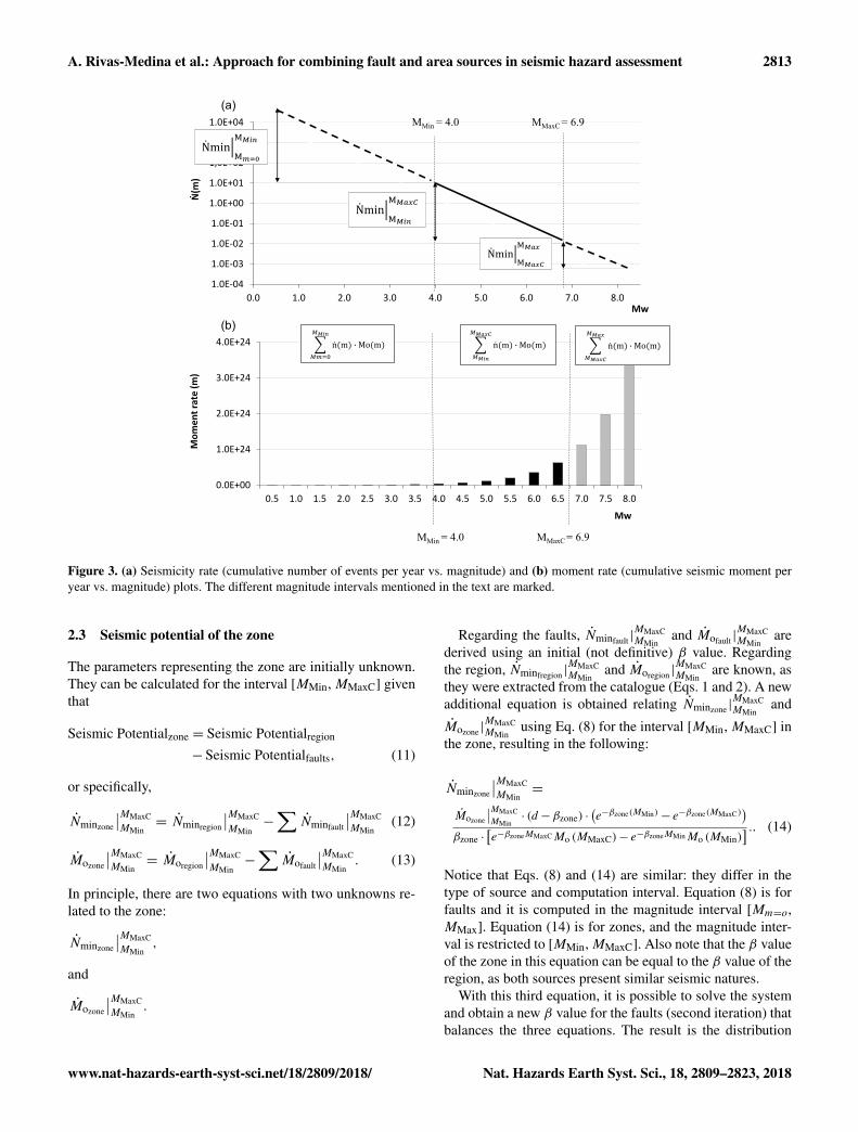
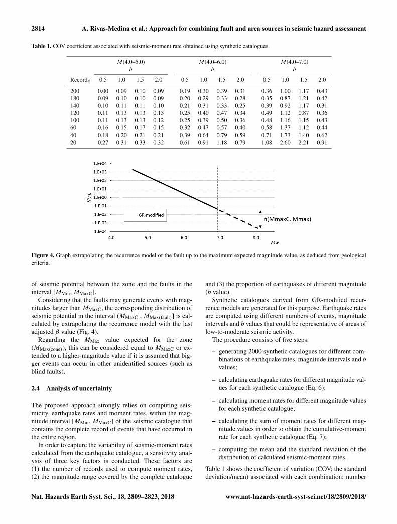
Table 1. COV coefficient associated with seismic-moment rate obtained using synthetic catalogues.

M(4.0–5.0) M(4.0–6.0) M(4.0–7.0)b b b

Records 0.5 1.0 1.5 2.0 0.5 1.0 1.5 2.0 0.5 1.0 1.5 2.0

200 0.00 0.09 0.10 0.09 0.19 0.30 0.39 0.31 0.36 1.00 1.17 0.43180 0.09 0.10 0.10 0.09 0.20 0.29 0.33 0.28 0.35 0.87 1.21 0.42140 0.10 0.11 0.11 0.10 0.21 0.31 0.33 0.25 0.39 0.92 1.17 0.31120 0.11 0.13 0.13 0.13 0.25 0.40 0.47 0.34 0.49 1.12 0.87 0.36100 0.11 0.13 0.13 0.12 0.25 0.39 0.50 0.36 0.48 1.16 1.15 0.4360 0.16 0.15 0.17 0.15 0.32 0.47 0.57 0.40 0.58 1.37 1.12 0.4440 0.18 0.20 0.21 0.21 0.39 0.64 0.79 0.59 0.71 1.73 1.40 0.6220 0.27 0.31 0.33 0.32 0.61 0.91 1.18 0.79 1.08 2.60 2.21 0.91

Figure 4. Graph extrapolating the recurrence model of the fault up to the maximum expected magnitude value, as deduced from geologicalcriteria.

of seismic potential between the zone and the faults in theinterval [MMin, MMaxC].

Considering that the faults may generate events with mag-nitudes larger than MMaxC, the corresponding distribution ofseismic potential in the interval (MMaxC , MMax(fault)] is cal-culated by extrapolating the recurrence model with the lastadjusted β value (Fig. 4).

Regarding the MMax value expected for the zone(MMax(zone)), this can be considered equal to MMaxC or ex-tended to a higher-magnitude value if it is assumed that big-ger events can occur in other unidentified sources (such asblind faults).

2.4 Analysis of uncertainty

The proposed approach strongly relies on computing seis-micity, earthquake rates and moment rates, within the mag-nitude interval [MMin, MMaxC] of the seismic catalogue thatcontains the complete record of events that have occurred inthe entire region.

In order to capture the variability of seismic-moment ratescalculated from the earthquake catalogue, a sensitivity anal-ysis of three key factors is conducted. These factors are(1) the number of records used to compute moment rates,(2) the magnitude range covered by the complete catalogue

and (3) the proportion of earthquakes of different magnitude(b value).

Synthetic catalogues derived from GR-modified recur-rence models are generated for this purpose. Earthquake ratesare computed using different numbers of events, magnitudeintervals and b values that could be representative of areas oflow-to-moderate seismic activity.

The procedure consists of five steps:

– generating 2000 synthetic catalogues for different com-binations of earthquake rates, magnitude intervals and bvalues;

– calculating earthquake rates for different magnitude val-ues for each synthetic catalogue (Eq. 6);

– calculating moment rates for different magnitude valuesfor each synthetic catalogue;

– calculating the sum of moment rates for different mag-nitude values in order to obtain the cumulative-momentrate for each synthetic catalogue (Eq. 7);

– computing the mean and the standard deviation of thedistribution of calculated seismic-moment rates.

Table 1 shows the coefficient of variation (COV; the standarddeviation/mean) associated with each combination: number



Figure 5. Three-dimensional view of the seismic sources considered for hazard calculation, including faults (red) and zones (brown).

of events, magnitude interval and b value. As can be seen, thegreater the number of records in the sample and the lower themagnitude range, the lower the uncertainty associated withthe rate of seismic moment calculated. The b value presents adifferent trend, recording the greatest variability for b valuesbetween 1.0 and 1.5. This table is useful for estimating theuncertainty of the seismic-moment rate calculated from theseismic catalogue as a function of the number of earthquakes,magnitude interval and b value.

It is also important to consider the uncertainty associatedwith the slip rate and the area of the fault, as these are prop-agated into the distribution of seismic-moment rates of thefault in proportion to the deviation of the area or slip ratevalue. The uncertainty of the slip rate value is more rele-vant for low slip rate values than for large slip rate values(a similar trend can be deduced for low and high area val-ues). For instance, a deviation of ±1 mm yr−1 in a slip rateof ±2 mm yr−1 represents an uncertainty of 50 %, leading toa COV value of 0.5 at the moment rate of the fault. However,the same deviation (±1 mm yr−1) for a fault with a slip rateof ±10 mm yr−1 represents an uncertainty of 10 %, leadingto a COV coefficient moment rate of only 0.1 for the fault.

3 Application of the approach in south-eastern Spain

The approach described above is applied in south-easternSpain, the most seismically active area in the country. Thetectonic deformation and seismicity is related to the north-western boundary between the Eurasian and African plates(e.g. Kiratzi and Papazachos, 1995), with an approximateshortening rate of about 4 mm yr−1 (Argus et al., 1989) ina roughly NNW–SSE direction. Crustal deformation is ac-cumulated over a broad area in which seismicity is diffuse(Benito and Gaspar-Escribano, 2007).

Assigning earthquakes to specific faults is not an easy task,partly due to errors in earthquake location and to the exis-tence of blind, unknown faults: whereas earthquakes can beclearly associated with a rupture, such as the 2011 M 5.2Lorca event generated in the Alhama de Murcia fault sys-tem (Cabañas et al., 2011), other events have occurred inareas where there are no mapped active faults, for instancethe 2007 Mw = 4.7 Pedro Muñoz and 2015 Mw = 4.7 Ossade Montiel earthquakes, both located in central Spain (QAFIdatabase, García-Mayordomo et al., 2012).

3.1 Source input data

The seismogenic source model considered for SE Spain iscomposed of 12 regions that contain a total of 95 faults(Supplement) Active fault data are taken from the QAFIdatabase (v2.0) (García-Mayordomo et al., 2012), which in-cludes information about fault segmentation, geometry andslip rate (see Fig. 5). The maximum expected magnitude ineach fault is derived from the rupture length using Stirling etal. (2002) equations derived from the instrumental data set.These equations are chosen because they are also the onesused in the QAFI database and ensure consistency with saiddatabase. Moment rates accumulated in the faults are esti-mated using the fault plane area and the slip rate value ac-cording to the formula proposed by Brune (1968). A value ofµ= 3.2×1010 Pa is assumed for the shear modulus (Walterset al., 2009; Martínez-Díaz et al., 2012).

The zone model proposed by García-Mayordomo etal. (2010) is used to obtain the geometries of the 12 regions(and thus of the zones) that account for the seismicity thatcannot be ascribed to faults (see Fig. 5). All the regions con-sidered in this model contain fault sources, with the excep-



Table 2. Seismic rate and seismic-moment rate recorded in the different regions for two magnitude intervals (MMin–MMax) and (MMin–MMaxC) obtained from the seismic catalogue. The table includes the ratio of seismic-moment rate of the two intervals, indicating whatpercentage of the seismic movement rate liberated from Mmin to Mmax is contemplated in the magnitude intervals over which hazard isdistributed (MMin–MMaxC). Note that no faults have been catalogued within regions 28, 29, 33 and 40, which is why no values have beenassigned (–).

Region MMin MMax MMaxC MMin–MMax MMin–MMaxC % Mo recorded in

N (4.0) Mo N (4.0) Mo complete periods(Nm yr−1) (Nm yr−1)

28 4.0 5.4 – 0.211 1.90× 1022 – – –29 4.0 6.2 – 0.176 7.90× 1022 – – –30 4.0 4.6 4.6 0.053 1.86× 1021 0.053 1.86× 1021 100 %31 4.0 6.5 5.7 0.241 7.88× 1022 0.239 4.70× 1022 60 %33 4.0 5.4 – 0.082 1.41× 1022 – – –34 4.0 6.3 5.5 0.219 3.28× 1022 0.218 2.56× 1022 78 %35 4.0 6.5 5.5 0.574 8.73× 1022 0.570 7.09× 1022 81 %36 4.0 6.2 5.4 0.142 2.21× 1022 0.141 1.41× 1022 64 %37 4.0 6.0 5.7 0.442 1.01× 1023 0.440 9.07× 1022 90 %38 4.0 6.5 5.4 0.527 6.75× 1022 0.525 5.70× 1022 84 %39 4.0 6.6 5.4 0.313 6.00× 1022 0.308 4.30× 1022 72 %40 4.0 6.0 – 0.135 4.06× 1022 – – –

tion of regions 28, 29, 33 and 40. In these cases, the seismicpotential of the corresponding region is assigned to the zones.

The seismic moment released in the region is estimatedfrom the seismic catalogue of Spain homogenized to Mw(IGN-UPM Working Group, 2013; Cabañas et al., 2015).This catalogue contains 1,496 earthquakes, with magnitudesranging from 4.0 to 6.6. The uncertainty assessment of thecatalogue used in this study is explained in Gaspar-Escribanoet al. (2015). According to the completeness analysis, aMMaxC of 5.9 is estimated for SE Spain (although not everyregion reaches this maximum-magnitude value). The recur-rence periods for magnitudes higher than 6 are too long toallow us to establish completeness periods for these magni-tude ranges (see Fig. 2).

Table 2 shows the seismic potential for each region, calcu-lated in the magnitude intervals [MMin, MMaxC] and [MMin,MMax(region)]. It is observed that the seismic potential in thefirst interval up to MMaxC, constitutes at least a 60 % of theseismic potential in the second interval, up to MMax(region).

Subsequently, a recurrence model (GR-mod) is assignedto all regions, obtaining the corresponding b values and COVcoefficients (see Table 3). Note that zone 30 lacks a COV es-timate because the sample of records (only 7) is very limited,and the [MMin, MMaxC] interval is very narrow, resulting inincreased uncertainty in the hazard estimates for this region.A GR-mod recurrence model is also assigned to the faults.Finally, the distribution of seismic moments among all seis-mic sources is carried out (Table 4). As may be observed, theseismic-moment rate associated with the zone has a stronginfluence on the estimated seismic hazard of the region. Thisis due to the limited number of known active faults that can

Table 3. Parameters extracted from the seismic catalogue for eachregion used to estimate the COV coefficient for Table 1, regions 28,29, 33 and 40 have been excluded because they contain no faults.

Region MMin MMaxC β-value Record COVregion

30 4.0 4.6 1.800 7 –31 4.0 5.7 1.980 66 0.434 4.0 5.5 2.345 35 0.635 4.0 5.5 2.242 117 0.336 4.0 5.4 2.400 25 0.737 4.0 5.7 1.917 83 0.338 4.0 5.4 2.240 85 0.339 4.0 5.4 1.750 61 0.3

be modelled as independent sources, a common situation inareas with low and moderate seismic activity. However, itis worth noting that the seismic potential of regions 35, 36and 38 is dominated by the seismic potential of faults.

The seismic hazard calculation is carried out using thesoftware CRISIS2012 (Ordaz et al., 2013), considering thestrong motion equation of Campbell and Bozorgnia (2014),which makes it possible to include the fault geometry andthe faulting style. The ground motion parameters predictedinclude peak ground acceleration (PGA) and 15 spectral ac-celerations within the period range (0.05–10 s), all obtainedin hard soil (Vs30 = 760 m s−1) conditions.



Table 4. Seismic potential distribution of faults and zones. The lastcolumn includes the percentage of regional seismic potential as-signed to each source within the region.

Region Source β value Nmin Mo(Nm yr−1)

306 fault 1.700 0.0078 2.76× 1020 15 %zone 1.800 0.0451 1.58× 1021 85 %Total 0.0529 1.86× 1021

316 fault 1.950 0.0372 7.37× 1021 16 %zone 1.980 0.2017 3.97× 1022 84 %Total 0.2389 4.70× 1022

346 fault 2.250 0.0244 2.92× 1021 11 %zone 2.345 0.1932 2.27× 1022 89 %Total 0.2176 2.56× 1022

356 fault 2.186 0.3474 4.33× 1022 61 %zone 2.242 0.2227 2.77× 1022 39 %Total 0.5701 7.09× 1022

366 fault 2.330 0.0804 8.02× 1021 57 %zone 2.400 0.0603 6.08× 1021 43 %Total 0.1407 1.41× 1022

376 fault 1.900 0.1247 2.57× 1022 28 %zone 1.917 0.3152 6.50× 1022 72 %Total 0.4399 9.07× 1022

386 fault 2.180 0.3269 3.55× 1022 62 %zone 2.240 0.2131 2.15× 1022 38 %Total 0.5400 5.70× 1022

396 fault 1.820 0.1005 1.35× 1022 31 %zone 1.750 0.2077 2.96× 1022 69 %Total 0.3082 4.30× 1022

3.2 Results

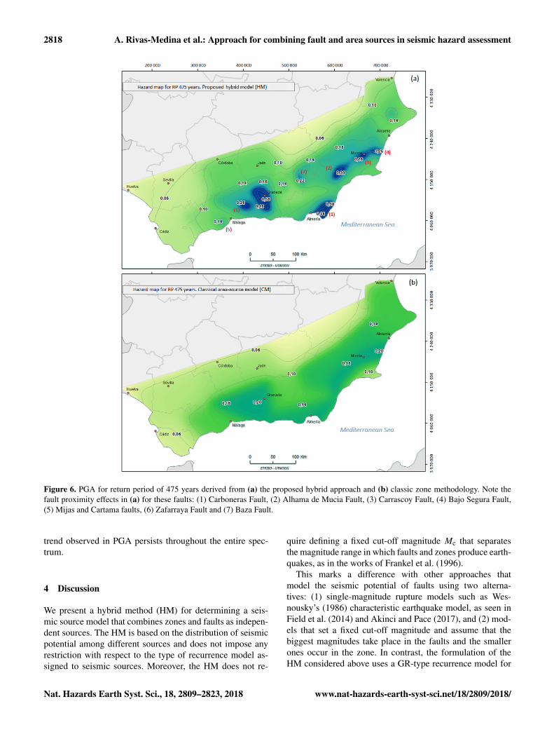
Seismic hazard results obtained with the proposed hy-brid model (HM) and with the classical method based inzone (CM) are shown in Fig. 6a and b. Only the geometry ofthe zone model differs in the two analyses: the ground mo-tion prediction equation (GMPE) and the other calculationparameters are the same in both approaches. The definitionof seismic zones applied in the classic method is explainedwith detail in IGN-UPM Working Group (2013).

PGA estimates for the return period of 475 years usingthe zone approach (CM) reach maximum values in Granada,Almeria and the Murcia region, around 0.20 g. MinimumPGA values are obtained in Jaén, with values as low as0.06 g.

Figure 6a shows the seismic hazard map resulting fromapplying our approach (HM). It can be seen that the largestaccelerations are estimated around the Carboneras Fault andthe fault set of Granada, (0.38 g), followed by the Alhama

de Murcia and La Viña faults systems (0.30 g) and, to a lesserextent, by the Venta de Zafarraya, Carrascoy, Bajo Segura,Baza, Mijas and Cartama fault systems.

The seismic hazard map obtained using the HM displaysmore spatial variability than the one obtained with the CM,showing maximum values along fault sources that decreasesharply away from the faults. This trend reflects a sourceproximity effect, implying higher acceleration values for thesurface projection of the fault rupture plane that rapidly de-crease away from the fault (by one half at a distance of about15 km).

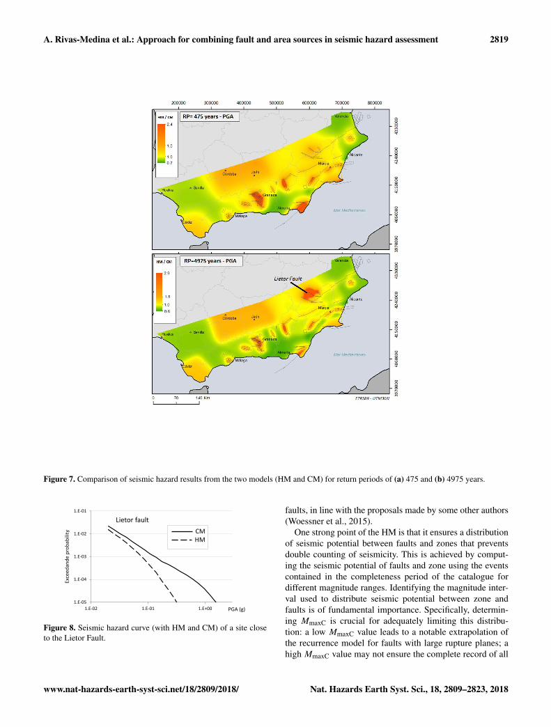
The differences between the expected maximum accelera-tion obtained with the two methods, CM and HM, for returnperiods of 475 and 4975 years appear in Fig. 7a and b. Thetrend presented in both maps is very similar for the two re-turn periods. A different case is found in region 30 (CaseLietor Fault), a very complex region with scarce seismic ac-tivity and large faults with low slip rates (see Supplement).Here, the HM gives higher seismic hazard than the CM onlyfor long return periods. For this region, the magnitude range[MMin, MMaxC] is very small and it is necessary to extrap-olate the model to a larger scale, given the high uncertaintyshown in Table 3. However, the results reflect that, for longerperiods, these slow faults play a relevant role in the seismichazard of the region (see Fig. 8), where the HM hazard curvereflects a substantial increase in hazard for long return peri-ods.

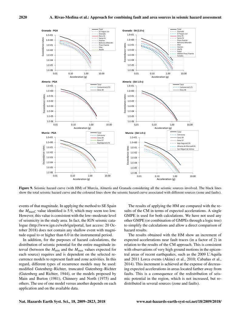
To clarify how faults are conditioning the final seismichazard in our model, the seismic hazard curves showing apartial contribution of different sources in Murcia, Almeriaand Granada are shown in Fig. 9 for PGA and SA (1.0 s). Foreach city, black lines show the total seismic hazard curve andcoloured lines show the seismic hazard curve associated withdifferent sources (zone and faults) for each city.

In Murcia, seismic hazard for short return periods is as-sociated with multiple sources (zone and faults), but for re-turn periods exceeding 475 years (an exceedance probabilityof 0.1 or lower in 50 years) the seismic hazard is dominatedby the Carrascoy Fault. This effect is very similar for PGAand SA (1.0 s).

In Almeria, only two sources, zone 38 and the CarbonerasFault, contribute significantly to seismic hazard. In PGA bothsources combine equally to give the seismic hazard for thecity, but, for SA (0.1 s), the Carboneras Fault predominates,especially for return periods of more than 475 years.

In Granada, there are many sources contributing to seismichazard for the city. This is because there are many knownfaults in its vicinity. Seismic hazard is controlled by zone 35for PGA and SA (1.0 s) and shorter return periods. This trendchanges for return periods greater than 975 years.

Figure 10 shows the uniform hazard spectra obtained forfour cities in the study area. These graphs can be used tocompare the maximum accelerations predicted with the CMand HM in different spectral ordinates, evidencing that the



Figure 6. PGA for return period of 475 years derived from (a) the proposed hybrid approach and (b) classic zone methodology. Note thefault proximity effects in (a) for these faults: (1) Carboneras Fault, (2) Alhama de Mucia Fault, (3) Carrascoy Fault, (4) Bajo Segura Fault,(5) Mijas and Cartama faults, (6) Zafarraya Fault and (7) Baza Fault.

trend observed in PGA persists throughout the entire spec-trum.

4 Discussion

We present a hybrid method (HM) for determining a seis-mic source model that combines zones and faults as indepen-dent sources. The HM is based on the distribution of seismicpotential among different sources and does not impose anyrestriction with respect to the type of recurrence model as-signed to seismic sources. Moreover, the HM does not re-

quire defining a fixed cut-off magnitude Mc that separatesthe magnitude range in which faults and zones produce earth-quakes, as in the works of Frankel et al. (1996).

This marks a difference with other approaches thatmodel the seismic potential of faults using two alterna-tives: (1) single-magnitude rupture models such as Wes-nousky’s (1986) characteristic earthquake model, as seen inField et al. (2014) and Akinci and Pace (2017), and (2) mod-els that set a fixed cut-off magnitude and assume that thebiggest magnitudes take place in the faults and the smallerones occur in the zone. In contrast, the formulation of theHM considered above uses a GR-type recurrence model for



Figure 7. Comparison of seismic hazard results from the two models (HM and CM) for return periods of (a) 475 and (b) 4975 years.

1.E-05

1.E-04

1.E-03

1.E-02

1.E-01

1.E-02 1.E-01 1.E+00

Exce

edan

de p

roba

bilit

y

PGA (g)

CMHM

Lietor fault

Figure 8. Seismic hazard curve (with HM and CM) of a site closeto the Lietor Fault.

faults, in line with the proposals made by some other authors(Woessner et al., 2015).

One strong point of the HM is that it ensures a distributionof seismic potential between faults and zones that preventsdouble counting of seismicity. This is achieved by comput-ing the seismic potential of faults and zone using the eventscontained in the completeness period of the catalogue fordifferent magnitude ranges. Identifying the magnitude inter-val used to distribute seismic potential between zone andfaults is of fundamental importance. Specifically, determin-ing MmaxC is crucial for adequately limiting this distribu-tion: a low MmaxC value leads to a notable extrapolation ofthe recurrence model for faults with large rupture planes; ahigh MmaxC value may not ensure the complete record of all



1.E-06

1.E-05

1.E-04

1.E-03

1.E-02

1.E-01

1.E+00

1.E+01

0.01 0.10 1.00 10.00

Exce

edan

ce ra

tes

Acceleration (g)

Granada - PGA TotalEl Fargue-JunGranadaZona 35Santa FéHuenesBelicena-AlhendínPinos PuenteDílarAtarfe

1.E-06

1.E-05

1.E-04

1.E-03

1.E-02

1.E-01

1.E+00

1.E+01

0.01 0.10 1.00 10.00

Exce

edan

ce ra

tes

Acceleration (g)

Granada - SA (1.0 s) TotalGranadaEl Fargue-JunZona 35Santa FéPinos PuenteBelicena-AlhendínDílarHuenesAtarfePadulObéilar-Pinos PuenteCanales

1.E-06

1.E-05

1.E-04

1.E-03

1.E-02

1.E-01

1.E+00

1.E+01

0.01 0.10 1.00 10.00

Exce

edan

ce ra

tes

Acceleration (g)

Almería - PGATotalCarboneras(1/2)Zona 38

1.E-06

1.E-05

1.E-04

1.E-03

1.E-02

1.E-01

1.E+00

1.E+01

0.01 0.10 1.00 10.00

Exce

edan

ce ra

tes

Acceleration (g)

Murcia - PGA TotalCarrascoyZona 39Zona 37BajoSegura(1/3)

1.E-06

1.E-05

1.E-04

1.E-03

1.E-02

1.E-01

1.E+00

1.E+01

0,01 0,10 1,00 10,00Ex

ceed

ance

rate

sAcceleration (g)

Almería - (SA 1.0 s)TotalCarboneras(1/2)Zona 38

1.E-06

1.E-05

1.E-04

1.E-03

1.E-02

1.E-01

1.E+00

1.E+01

0.01 0.10 1.00 10.00

Exce

edan

ce ra

tes

Acceleration (g)

Murcia - (SA 1.0 s) TotalCarrascoyZona 39Zona 37Bajo Segura(1/3)Alhama de Murcia(4/4)San Miguel de Salinas

Figure 9. Seismic hazard curve (with HM) of Murcia, Almería and Granada considering all the seismic sources involved. The black linesshow the total seismic hazard curve and the coloured lines show the seismic hazard curve associated with different sources (zone and faults).

events of that magnitude. In applying the method to SE Spainthe MmaxC value identified is 5.9, which may seem too low.However, this value is consistent with the low–moderate levelof seismicity in the study area. In fact, the IGN seismic cata-logue (http://www.ign.es/web/ign/portal, last access: 20 Oc-tober 2018) does not contain any shallow event with magni-tude equal to or higher than 6.0 in the instrumental period.

In addition, for the purposes of hazard calculations, thedistribution of seismic potential for the entire magnitude in-terval (between the Mmin and the Mmax values expected foreach source) requires and is dependent on the selected re-currence models to represent fault and zone activities. In thisregard, different types of recurrence models may be used:modified Gutenberg–Richter, truncated Gutenberg–Richter(Gutenberg and Richter, 1944), or the models proposed byMain and Burton (1981), Chinnery and North (1975) andothers. The use of one model versus another depends on eachapplication and on the available data.

The results of applying the HM are compared with the re-sults of the CM in terms of expected accelerations. A singleGMPE is used for both calculations. We have not used anyother GMPE (or combination of GMPEs through a logic tree)to simplify the calculations and allow a direct comparison ofhazard results.

The results obtained with the HM show an increment ofexpected accelerations near fault traces (in a factor of 2) inrelation to the results of the CM approach. This is consistentwith observations of very high ground motions in the epicen-tral areas of recent earthquakes, such as the 2009 L’Aquilaand 2011 Lorca events (Akinci et al., 2010; Cabañas et al.,2014). This increment is achieved at the expense of decreas-ing expected accelerations in areas located farther away fromfaults. This is a consequence of the redistribution of seis-mic potential in the region, which is not increased, but re-distributed in several sources (zone and faults).


http://www.ign.es/web/ign/portal


Figure 10. Uniform hazard spectra obtained in four cities with CM and HM for three return periods.

5 Conclusions

An approach for combining zones and faults in a seismicsource model is formulated in this paper.

It is based on the distribution of seismic potential amongdifferent sources under certain conditions to prevent count-ing seismicity twice. Two points of the methodology are crit-ical and must be carefully assessed: the analysis of complete-ness and the choice of recurrence model used to represent theseismic activity of either source. They are determined by thedata available (composition of the seismic catalogue, faultslip rates and geometries, etc.) in the study region, and hencenot easily automatized and extendible to other areas. Thus,the approach followed for the application in SE Spain shouldbe reevaluated when it is applied to a different area. For in-stance, it is to be expected that implementing this approachin a region with rapidly moving faults would produce signif-icantly different results, requiring further adjustments. Thehigher fault slip rates would imply that the faults consume alarger proportion of the seismic potential available, compro-mising the convergence of the iterative method to obtain thezone β value.

An initial assumption of the approach is that the seismic-moment potential accumulated in active faults is releasedonly seismically. This condition can be easily modified inthe formulation presented above. Additional data informing

about other ways of releasing seismic energy, such as slowslip events or aseismic transients, would help to constrain thispoint.

The seismic hazard map obtained with the HM presents amore heterogeneous aspect compared to the CM seismic haz-ard map, which assigns a uniform seismic potential to eachregion. In the HM hazard map, the accelerations expectedalong fault traces increase and decrease farther away fromfault traces, thus keeping the seismic potential budget of theregion in balance. This effect can be useful for applicationsin which the effects of being near a fault must be emphasized,such as urban seismic risk studies for cities located atop ac-tive fault planes.

As a final conclusion, we identify some points that requirefurther development and are the focus of an interesting lineof research. Specifically, these include (1) determining cata-logue completeness for different time-magnitude intervals inthe study area; (2) selecting the recurrence model assignedto fault sources according to the data available, and (3) de-termining the proportion of seismic potential accumulated infaults that is released through earthquakes.

Data availability. The available data of active faults are in the Sup-plement.



Supplement. The supplement related to this article is availableonline at: https://doi.org/10.5194/nhess-18-2809-2018-supplement.

Author contributions. All authors contributed to the preparation ofthis paper.

Competing interests. The authors declare that they have no conflictof interest.

Acknowledgements. We would like to thank Mario Or-daz Schroeder for his time and support during a researchstay carried out by ARM at the Instituto de Ingeniería, UNAM,and we acknowledge financial support from Vicerrectoría deInvestigación y Desarrollo (VRID), UdeC, “216.419.003-1.0IN”.

Edited by: Maria Ana BaptistaReviewed by: five anonymous referees

References

Akinci, A. and Pace, B.: Effect of Fault Parameter Uncertainties onPSHA explored by Monte Carlo Simulations: A case study forsouthern Apennines, Italy, in: AGU Fall Meeting Abstracts, 11–15 December 2017, New Orleans, 2017.

Akinci, A., Malagnini, L., and Sabetta, F.: Characteristics of thestrong ground motions from the 6 April 2009 L’Aquila earth-quake, Italy, Soil Dynam. Earthq. Eng., 30, 320–335, 2010.

Anderson, J. G. and Luco, J. E.: Consequences of slip rate con-straints on earthquake occurrence relations, B. Seismol. Soc.Am., 73, 471–496, 1983.

Argus, D. F., Gordon, R. G., DeMets, C., and Stein, S.: Closureof the Africa–Eurasia–North America plate motion circuit andtectonics of the Gloria Fault, J. Geophys. Res., 94, 5585–5602,1989.

Basili, R., Tiberti, M. M., Kastelic, V., Romano, F., Piatanesi, A.,Selva, J., and Lorito, S.: Integrating geologic fault data intotsunami hazard studies, Nat. Hazards Earth Syst. Sci., 13, 1025–1050, https://doi.org/10.5194/nhess-13-1025-2013, 2013.

Benito, M. B. and Gaspar-Escribano, J. M.: Ground Motion Charac-terization in Spain: Context, Problems and Recent Developmentsin Seismic Hazard Assessment, J. Seismol., 11, 433–452, 2007.

Benito, M. B., Navarro, M., Vidal, F., Gaspar-Escribano, J., García-Rodríguez, M. J., and Martínez-Solares, J. M.: A new seismichazard assessment in the region of Andalusia (Southern Spain),B. Earthq. Eng., 8, 739–766, 2010.

Brune, J. N.: Seismic moment, seismicity, and rate of slipalong major fault zones, J. Geophys. Res., 73, 777–784,https://doi.org/10.1029/jb073i002p00777, 1968.

Bungum, H.: Numerical modelling of fault activities, Comput.Geosci., 33, 808–820, 2007.

Cabañas Rodríguez, L., Carreño Herrero, E., Izquierdo Álvarez, A.,Martínez Solares, J. M., Capote del Villar, R., Martínez Díaz,J., Benito Oterino, B., Gaspar Escribano, J., Rivas Medina, A.,García Mayordomo, J., Pérez López, R., Rodríguez Pascua, M.A., and Murphy Corella, P.: Informe del sismo de Lorca del 11 de

mayo de 2011, Instituto Geográfico Nacional, Madrid, p. 138,2011.

Cabañas, L., Alcalde, J. M., Carreño, E., and Bravo, J. B.: Char-acteristics of observed strong motion accelerograms from the2011 Lorca (Spain) Earthquake, B. Earthq. Eng., 12, 1909–1932,2014.

Cabañas, L., Rivas-Medina, A., Martínez-Solares, J. M., Gaspar-Escribano, J. M., Benito, B., Antón, R., and Ruiz-Barajas, S.: Re-lationships between Mw and Other Earthquake Size Parametersin the Spanish IGN Seismic Catalog, Pure Appl. Geophys., 172,2397–2410, https://doi.org/10.1007/s00024-014-1025-2, 2015.

Campbell, K. W. and Bozorgnia, Y.: NGA-West2 ground motionmodel for the average horizontal components of PGA, PGV, and5 % damped linear acceleration response spectra, Earthq. Spec-tra., 30, 1087–1115, https://doi.org/10.1193/062913eqs175m,2014.

Chinnery, M. A. and North, R. G.: The frequency of very largeearthquakes, Science, 190, 1197–1198, 1975.

Crespo, M. J., Martínez, F., and Martí, J.: Seismic hazard of theIberian Peninsula: evaluation with kernel functions, Nat. HazardsEarth Syst. Sci., 14, 1309–1323, https://doi.org/10.5194/nhess-14-1309-2014, 2014.

DISS Working Group: Database of Individual SeismogenicSources (DISS), Version 3.2.1, A compilation of potentialsources for earthquakes larger than M 5.5 in Italy and sur-rounding areas, Istituto Nazionale di Geofisica e Vulcanologia,https://doi.org/10.6092/INGV.IT-DISS3.2.1, 2018.

Dixon, T. H., Norabuena, E., and Hotaling, L.: Paleoseismology andGlobal Positioning System: Earthquake-cycle effects and geode-tic versus geologic fault slip rates in the Eastern California shearzone, Geology, 31, 55–58, 2003.

Field, E. H., Arrowsmith, R. J., Biasi, G. P., Bird, P., Dawson, T. E.,Felzer, K. R., Jackson, D. D., Johnson, K. M., Jordan, T. H., Mad-den, C., Michael, A. J., Milner, K. R., Page, M. T., Parsons, T.,Powers, P. M., Shaw, B. E., Thatcher, W. R., Weldon, R. J., andZeng, Y.: Uniform California Earthquake Rupture Forecast, Ver-sion 3 (UCERF3) – The Time-Independent Model, B. Seismol.Soc. Am., 104, 1122–1180, https://doi.org/10.1785/0120130164,2014.

Frankel, A. D., Mueller, C., Barnhard, T., Perkins, D., Leyendecker,E., Dickman, N., Hanson, S., and Hopper, M.: National seismic-hazard maps: documentation June 1996, US Geological Survey,Denver, https://doi.org/10.3133/ofr96532, 1996.

García-Mayordomo, J.: Caracterización y Análisis de la Peligrosi-dad Sísmica en el Sureste de España, PhD Thesis, UniversityComplutense of Madrid, Madrid, Spain, 2005.

García-Mayordomo, J., Gaspar-Escribano, J. M., and Benito, B.:Seismic hazard assessment of the Province of Murcia (SE Spain):analysis of source contribution to hazard, J. Seismol., 11, 453–471, 2007.

García-Mayordomo, J., Insua-Arévalo, J. M., Martínez-Díaz, J. J.,Perea, H., Álvarez-Gómez, J. A., Martín-González, F., González,A., Lafuente, P., Pérez-López, R., Rodríguez-Pascua, M. A.,Ginez-Robles, J., and Azañón, J. M.: Modelo integral de zonassismogénicas de España, in: Contribución de la Geología alAnálisis de la Peligrosidad Sísmica, edited by: Insua-Arévalo,J. M. y Martín-González, J. J., Sigüenza, Guadalajara, España,193–196, 2010.


https://doi.org/10.5194/nhess-18-2809-2018-supplement

https://doi.org/10.5194/nhess-13-1025-2013

https://doi.org/10.1029/jb073i002p00777

https://doi.org/10.1007/s00024-014-1025-2

https://doi.org/10.1193/062913eqs175m



https://doi.org/10.6092/INGV.IT-DISS3.2.1

https://doi.org/10.1785/0120130164

https://doi.org/10.3133/ofr96532


García-Mayordomo, J., Insua-Arévalo, J. M., Martínez-Díaz, J.J., Jiménez-Díaz, A., Martín-Banda, R., Martín-Alfageme, S.,Álvarez-Gómez, J. A., Rodríguez-Peces, M., Pérez-López, R.,Rodríguez-Pascua, M. A., Masana, E., Perea, H., Martín-González, F., Giner-Robles, J., Nemser, E. S., and Cabral, J.: Thequaternary active faults database of iberia (QAFI v.2.0)/La basede datos de fallas activas en el cuaternario de iberia (QAFI v.2.0),J. Iber. Geol., 38, 285–302, 2012.

Gaspar-Escribano, J. M., Rivas-Medina, A., Parra, H., Cabañas, L.,Benito, B., Barajas, S. R., and Solares, J. M.: Uncertainty as-sessment for the seismic hazard map of Spain, Eng. Geol., 199,62–73, https://doi.org/10.1016/j.enggeo.2015.10.001, 2015.

Gutenberg, B. and Richter, C. F.: Frequency of earthquakes in Cali-fornia, B. Seismol. Soc. Am., 34, 185–188, 1944.

Hakimhashemi, A. H. and Grünthal, G.: A statistical method forestimating catalog completeness applicable to long-term nonsta-tionary seismicity data, B. Seismol. Soc. Am., 102, 2530–2546,2012.

Hanks, T. C. and Kanamori, H.: A moment magnitude scale, J. Geo-phys. Res., 84, 23480–23500, 1979.

IGN-UPM working group: Actualización de mapas de peligrosidadsísmica de España 2012, Centro Nacional de Información Ge-ográfica, Madrid, 267 pp., 2013.

Kijko, A., Smit, A., and Sellevoll, M. A.: Estimation of earthquakehazard parameters from incomplete data files. Part III. Incorpo-ration of uncertainty of earthquake-occurrence model, . Seismol.Soc. Am., 106, 1210–1222, 2016.

Kiratzi, A. A. and Papazachos, C. B.: Active crustal deformationfrom the Azores triple junction to the Middle East, Tectono-physics, 243, 1–24, 1995.

Langbein, J. and Bock, Y.: High-rate real-time GPS net-work at Parkfield: Utility for detecting fault slip andseismic displacements, Geophys. Res. Lett., 31, L15S20,https://doi.org/10.1029/2003GL019408, 2004.

Leonard, M.: Earthquake Fault Scaling: Self-Consistent Relat-ing of Rupture Length, Width, Average Displacement, andMoment Release, B. Seismol. Soc. Am., 100, 1971–1988,https://doi.org/10.1785/0120120249, 2010.

Main, I. G. and Burton, P. W.: Rates of crustal deformation inferredfrom seismic moment and Gumbel’s third distribution of extrememagnitude values, in: Earthquakes and Earthquake Engineering:The Eastern United States, edited by: Beavers, J. E., Ann ArborScience, Michigan, 937–951, 1981.

Martínez-Díaz, J. J., Bejar-Pizarro, M., Álvarez-Gómez, J. A.,de Lis Mancilla, F., Stich, D., Herrera, G., and Morales, J.: Tec-tonic and seismic implications of an intersegment rupture: Thedamaging May 11th 2011 Mw 5.2 Lorca, Spain, earthquake,Tectonophysics, 546, 28–37, 2012.

Metzger, S., Jónsson, S., and Geirsson, H.: Locking depth and slip-rate of the Húsavík Flatey fault, North Iceland, derived from con-tinuous GPS data 2006–2010, Geophys. J. Int., 187, 564–576,2011.

Mezcua, J., Rueda, J., and Blanco, R. M. G.: A new probabilis-tic seismic hazard study of Spain, Nat. Hazards, 59, 1087–1108,2011.

Nasir, A., Lenhardt, W., Hintersberger, E., and Decker, K.: Assess-ing the completeness of historical and instrumental earthquakedata in Austria and the surrounding areas, Aust. J. Earth. Sci.,106, 90–102, 2013.

Ordaz, M., Martinelli, F., D’Amico, V., and Meletti, C.: CRI-SIS2008: A Flexible Tool to Perform Probabilistic Seis-mic Hazard Assessment, Seismol. Res. Lett., 84, 495–504,https://doi.org/10.1785/0220120067, 2013.

Papanikolaou, I. D., Roberts, G. P., and Michetti, A. M.: Fault scarpsand deformation rates in Lazio–Abruzzo, Central Italy: Compar-ison between geological fault slip-rate and GPS data, Tectono-physics, 408, 147–176, 2005.

Parsons, T. and Geist, E. L.: Is there a basis for preferring char-acteristic earthquakes over a Gutenberg–Richter distribution inprobabilistic earthquake forecasting?, B. Seismol. Soc. Am., 99,2012–2019, 2009.

Peláez, J. A. and Lopez-Casado, C.: Seismic Hazard estimate at theIberian Peninsula, Pure Appl. Geophys., 159, 2699–2713, 2002.

Salgado-Gálvez, M. A., Cardona, O. D., Carreño, M. L., and Bar-bat, A. H.: Probabilistic seismic hazard and risk assessment inSpain, Centro Internacional de Métodos Numéricos en Inge-niería, Barcelona, 2015.

Stirling, M., Rhoades, D., and Berryman, K.: Comparison of earth-quake scaling relations derived from data of the instrumentaland preinstrumental era, B. Seismol. Soc. Am., 92, 812–830,https://doi.org/10.1785/0120000221, 2002.

Walpersdorf, A., Manighetti, I., Mousavi, Z., Tavakoli, F.,Vergnolle, M., Jadidi, A., Hatzfeld, D., Aghamohammadi, A.,Bigot, A., Djamour, Y., Nankali, H., and Sedighi, M.: Present-day kinematics and fault slip rates in eastern Iran, derived from11 years of GPS data, J. Geophys. Res.-Solid, 119, 1359–1383,2014.

Walters, R. J., Elliott, J. R., D’agostino, N., England, P. C., Hunstad,I., Jackson, J. A., Parsons, B., Phillips, R. J., and Roberts, G.:The 2009 L’Aquila earthquake (central Italy): A source mecha-nism and implications for seismic hazard, Geophys. Res. Lett.,36, L17312, https://doi.org/10.1029/2009GL039337, 2009.

Wells, D. L. and Coppersmith, K. J.: New empirical relationshipsamong magnitude, rupture length, rupture width, rupture area,and surface displacement, B. Seismol. Soc. Am., 84, 974–1002,1994.

Wesnousky, S. G.: Earthquakes, Quatemary faults, and seismic haz-ard in California, J. Geophys. Res., 91, 12587–12631, 1986.

Woessner, J., Laurentiu, D., Giardini, D., Crowley, H., Cotton, F.,Grünthal, G., Valensise, G., Arvidsson, R., Basili, R., Demir-cioglu, M. B., Hiemer, S., Meletti, C., Musson, R. W., Rovida,A. N., Sesetyan, K., Stucchi, M., and The SHARE Consortium::The 2013 European seismic hazard model: key components andresults, B. Earthq. Eng., 13, 3553–3596, 2015.


https://doi.org/10.1016/j.enggeo.2015.10.001

https://doi.org/10.1029/2003GL019408

https://doi.org/10.1785/0120120249

https://doi.org/10.1785/0220120067

https://doi.org/10.1785/0120000221

https://doi.org/10.1029/2009GL039337

approach for combining fault and area sources in seismic

Documents