See discussions, stats, and author profiles for this publication at: https://www.researchgate.net/publication/5157518

Applying Portfolio Change and Conditional Performance Measures: The Case of

Industry Rotation via the Dynamic Investment Model

Article  in  Review of Quantitative Finance and Accounting · February 2001

DOI: 10.1023/A:1012240609470 · Source: RePEc

CITATIONS

18READS

57

2 authors, including:

Robert R. Grauer

Simon Fraser University

52 PUBLICATIONS   1,501 CITATIONS   

SEE PROFILE

All content following this page was uploaded by Robert R. Grauer on 24 July 2017.

The user has requested enhancement of the downloaded file.

Applying Portfolio Change and Conditional Performance Measures: The Case of Industry Rotation via the Dynamic Investment Model* †

by

Robert R. Grauer Faculty of Business Administration

Simon Fraser University 8888 University Drive

Burnaby, B.C., Canada V5A 1S6 Phone: (604) 291-3722 Fax: (604) 291-4920 Email: grauer@sfu.ca

and

Nils H. Hakansson

Haas School of Business University of California, Berkeley

545 Student Services Building Berkeley, California 94720-1900

Phone: (510) 642-1686 Fax: (510) 643-8460

Email: hakansso@haas.berkeley.edu

Latest version March 2001 Forthcoming in the Review of Quantitative Finance and Accounting

* Financial support from the Social Sciences and Humanities Research Council of Canada is gratefully acknowledged. The authors are indebted to Reo Audette, Poh Chung Fong, John Janmaat, and William Ting for valuable research assistance and to Gero Goetzenberger, Maciek Kon, and Derek Lai for programming assistance.

† An earlier version was presented at the Sixth Conference on Pacific Basin Business, Economics and Finance in Hong Kong, the European Finance Association Meetings in Fontainebleau, and the Northern Finance Association Meetings in Toronto. The comments of Wayne Ferson, Elisa Luciano, and Jay Shanken were especially valuable.

Applying Portfolio Change and Conditional Performance Measures:

The Case of Industry Rotation via the Dynamic Investment Model

Abstract

This paper applies portfolio change and conditional performance measures to assess the

performance of the dynamic investment model in various industry-rotation settings spanning the

1934-1995 period. The dynamic investment model employs the empirical probability assessment

approach in raw form. In addition, it incorporates three adjustments for estimation error: James-

Stein, Bayes-Stein, and CAPM-based corrections. The tests are unanimous in their conclusion

that the excess returns attained by the (unadjusted) historic, the Bayes-Stein, and the James-Stein

estimators are (sometimes highly) statistically significant over the 1966-95 and 1966-81 sub-

periods. This lends support to the idea that the joint empirical probability assessment approach

based on the recent past, with and without Stein-based corrections for estimation error, contains

information that can be profitably exploited. The relationship of these findings to the extant

literature on momentum and contrarian strategies is addressed.

1

I. Introduction

Based on traditional performance measures, the discrete-time dynamic investment model in

conjunction with the empirical probability assessment approach (EPAA) shows a surprising

amount of mettle. In particular, Jensen's (1968) test of microforecasting, the Treynor and Mazuy

(1966) and Henriksson and Merton (1981) tests of macroforecasting, and a paired t-test of the

difference in geometric mean returns indicate that the model performs well, both with and

without adjustment for estimation risk, in a number of different environments. See, for example,

Grauer and Hakansson (1986, 1987, 1995a, 1995b, 1998) and Grauer, Hakansson and Shen

(1990). However, traditional performance measures are not without their critics. Roll (1978)

argues that the measures of performance (alphas) and risk (betas) are sensitive to the choice of a

proxy for the market portfolio. Moreover, Cheng and Grauer (1980) and Grauer (1991) point out

some of the problems associated with assuming constant betas.

Two recently introduced tests add new dimensions to the performance measurement process.

Grinblatt and Titman's (1993) portfolio change measure, which focuses on portfolio holdings as

well as investment returns, avoids using a proxy for the market portfolio. The second category

of tests, introduced by Shanken (1990) and extended to the investment performance literature by

Ferson and Schadt (1996), are generally referred to as conditional performance measures. These

tests attempt to untangle performance attributable to public information from that which is not.

By incorporating betas which are time-varying due to market indicators such as lagged dividend

yields and Treasury bill rates, these measures take account of any implied comovement between

expected returns and risk.

This paper applies Grinblatt and Titman's (1993) portfolio change measure and Ferson and

Schadt's (1996) conditional performance measures to assess the performance of the dynamic

2

investment model in various industry-rotation settings spanning the 1934-1995 period. In

choosing its portfolio holdings, the dynamic investment model employs the EPAA, with a rear-

view moving window, in raw form and with three adjustments for estimation error: a James-

Stein, a Bayes-Stein, and a CAPM-based correction. 1

In contrast to the typical approach to the study of estimation risk and momentum effects, this

paper examines the portfolio selection problem in the asset allocation format so familiar to real-

world investment managers. In particular, the present analysis differs from previous studies on

several dimensions:

• The model used is based on (discrete-time) dynamic investment theory rather than on single-

period portfolio theory. (In this model, the optimal mix of risky assets is sensitive to the risk

attitude, in contrast to the case in the mean-variance framework.)

• Portfolios are revised quarterly.

• Short sales are ruled out.

• A risk-free asset (90-day Treasury Bills) is available each period.

• Borrowing is permitted up to posted margin requirements (at a rate higher than the

contemporary lending rate.)

• The estimation or formation period is 32 quarters, far longer than in other studies.

• A wide range of risk attitudes is examined.

On the other hand, the present study has the following properties in common with related

inquiries:

• The investor is viewed as a price-taker – no particular equilibrium model is assumed or

relevant.

• “Standard” approaches are employed in measuring investment performance.

3

The main results may be summarized as follows. The conditional tests give higher

performance ratings than the unconditional ones without exception. The Grinblatt-Titman test

and the conditional Jensen, Henriksson-Merton, and Treynor-Mazuy tests (as well as the naked

eye test applied to Figures 1-3) come to the conclusion that the excess returns attained by the

(unadjusted) historic, the Bayes-Stein, and the James-Stein estimators are (sometimes highly)

statistically significant over the 1966-95 and 1966-81 sub-periods but, except for the conditional

Jensen test, not over the full 1934-95 period. These results hold both when the industry

components are value-weighted and when they are equal-weighted. Only the Treynor-Mazuy

conditional test judges the CAPM estimator's excess returns to be significant over the two sub-

periods.

II. The Dynamic Investment Model

The basic model used is the same as the one employed in Grauer and Hakansson (1986,

1998) and the reader is therefore referred to those papers for details. It is based on the pure

reinvestment version of dynamic investment theory. In particular, if )( nn wU is the induced

utility of wealth nw with n periods to go (to the horizon) for a risk-averse investor and r is the

single-period return, the important convergence result (Hakansson (1974); see also Leland

(1972), and Huberman and Ross (1983))

1, somefor ,1)( <→ γγ

γwwUn

holds for a very broad class of risk-averse terminal utility functions )( 00 wU when returns are

independent, whether stationary or nonstationary, from period to period. Convergence implies

that, when the horizon is distant, use of the stationary, myopic decision rule

1, somefor ,)1(1max <

+ γγ

γrE (1)

4

in each period is optimal. Consequently, the family of decision rules (1) encompasses a broad

variety of different goal formulations for investors with intermediate- to long-term investment

horizons.2 Since the relative risk aversion function (-wU"(w)/U'(w)) for (1) is γ−1 , the family

(1) incorporates the full range of risk attitudes from (near) zero to infinity.

More specifically, at the beginning of each period t, the investor chooses a portfolio, tx , on

the basis of some member γ of the family of objective (or utility) functions (1) subject to the

relevant constraints faced by the investor. This is equivalent to solving the following problem in

each period t:

γγ

γπ

γ))(1(1max))(1(1max tts

stsxttx

xrxrEtt

+∑=

+ (2)

subject to

, all,0,0,0 ixxx BtLtit ≤≥≥ (3)

,1∑ =++i

BtLtit xxx (4)

∑ ≤i

itit xm ,1 (5)

,1)0)(1Pr( =≥+ tt xr (6)

where

∑ ++=i

dBtBtLtLtitsittts rxrxrxxr )( is the (ex ante) return on the portfolio in period t if state s

occurs,

γ = the risk-aversion parameter (which remains fixed over time),

itx = the amount invested in risky asset category i in period t as a fraction of own capital,

Ltx = the amount lent in period t as a fraction of own capital,

5

Btx = the amount borrowed in period t as a fraction of own capital,

tx = ,),,,...,( 1 ′BtLtntt xxxx 3

itr = the anticipated total return (dividend yield plus capital gains or losses) on asset category

i in period t,

dBtr = the interest rate on borrowing at the time of the decision at the beginning of period t,

itm = the initial margin requirement for asset category i in period t expressed as a fraction,

and

tsπ = the probability of state s at the end of period t, in which case the random return itr will

assume the value itsr .

As noted, the myopic objective function (2) assumes that returns from period to period are

independent (but not that they are stationary) while the evidence suggests that quarterly real-

world equity returns may be only nearly independent. (Whether the resulting loss from

employing a myopic decision rule is significant will be addressed in a later study.) Constraint (3)

rules out short sales and (4) is the budget constraint. Constraint (5) serves to limit borrowing

(when desired) to the maximum permissible under the margin requirements that apply to the

various asset categories. Finally, constraint (6) rules out any (ex ante) probability of

bankruptcy.4

The inputs to the model are based on the "empirical probability assessment approach"

(EPAA) or a variant thereof. Consider the EPAA and suppose quarterly revision is used. Then,

at the beginning of quarter t, the portfolio problem (2)-(6) for that quarter uses the following

inputs: the (observable) riskfree return for quarter t, the (observable) call money rate +1 percent

at the beginning of quarter t, and the (observable) realized returns for the risky asset categories

6

for the previous k quarters. Each joint realization in the estimation or formation period, quarters

t-k through t-1, is given probability 1/k of occurring in quarter t. Thus, under the EPAA,

estimates are obtained on a moving basis and used in raw form without adjustment of any kind.

On the other hand, since the objective function (2) requires that the whole joint distribution be

specified and used, as noted earlier, there is no information loss; all moments and correlations

are implicitly taken into account.

In this study, the estimation period k was set to 32 quarters on an a priori basis. This choice

was dictated by a compromise between two criteria: the need for a long enough period to attain

representativeness of past returns - but not too long in light of the apparent nonstationarity of

equity returns. No other value of k was examined.

With these inputs in place, the portfolio weights tx for the various asset categories and the

proportion of assets borrowed were calculated by solving system (2)-(6) via nonlinear

programming methods.5 At the end of quarter t, the realized returns on the risky assets were

observed, along with the realized borrowing rate rBtr (which may differ from the decision

borrowing rate dBtr ).6 Then, using the weights selected at the beginning of the quarter, the

realized return on the portfolio chosen for quarter t was recorded. The cycle was then repeated in

all subsequent quarters.7

All reported returns are gross of transaction costs and taxes and assume that the investor in

question had no influence on prices. One reason for the former is that the return series used as

inputs and for comparisons also exclude transaction costs (for reinvestment of interest and

dividends) and taxes.

7

III. Correcting the Model for Estimation Error

Ex ante means are difficult to estimate and the solution to the portfolio problem is generally

extremely sensitive to changes in the means (see Best and Grauer (1991)). Furthermore, the

estimation risk literature suggests that we should be able to improve investment performance

(substantially) by using better forecasts of the means.8 Therefore, this study compares the

investment performance of the dynamic investment model under three classes of estimators of

the means: the EPAA means; the shrinkage or James-Stein and Bayes-Stein estimators of the

means, which are based on statistical models; and the CAPM-based estimator of the means,

which is based on a model of market equilibrium. No adjustment is made to the EPAA variance-

covariance structure or to the other moments.

Under the EPAA approach, means are not used directly but are implicitly computed from the

realized returns. We denote the n-vector of historic (EPAA) means at the beginning of period t as

( )ntitHt r,,r !=µ ', (7)

where ∑−

−=

=11 t

ktiit r

kr

ττ . The EPAA approach implicitly estimates the means one at a time, relying

exclusively on information contained in each of the time series. Stein's (1955) suggestion that

the efficiency of the estimate of the means could be improved by pooling the information across

series leads to a number of so-called "shrinkage" estimators that shrink the historical means to

some grand mean. A classic example is the James-Stein (JS) estimator, which takes the form9

,)1( ιµµ GttHttJSt rww +−= (8)

where ))]()(/()2(,1min[ 1 ιµιµ GtHttGtHtt rSrknw −′−−= − is the shrinking factor, tS is the sample

covariance matrix calculated from the k periods in the estimation period, ∑=i

itGt rn

r 1 is the

8

grand mean, and ι is a vector of ones. In this case, the simple historic means are "shrunk"

toward the arithmetic average of the historic means.10, 11

A second example is Jorion's (1985, 1986, 1991) Bayes-Stein (BS) estimator

ιµµ GttHttBSt rww +−= )1( , (9)

where ),/( kw ttt += λλ ))()/(()2( 1 ιµιµλ GtHttGtHtt rSrn −′−+= − , and )./( 11 ιιµι −− ′′= tHttGt SSr In

this case, the grand mean is the mean of the global minimum-variance portfolio generated from

the historical data.

The second alternative class of estimators of the means is borrowed from the Sharpe (1964) -

Lintner (1965) CAPM, a model of market equilibrium.12 The CAPM estimator of the means is

,)( tLtmtLtCAPMt rrr βιµ −+= (10)

where ∑−

−=

=11 t

ktmmt r

kr

ττ and ,1 1

∑−

−=

=t

ktLLt r

kr

ττ so that Ltmt rr − is an estimate of the expected excess

return on the market portfolio, and ),,( 1 nttt βββ "= ' is the vector of betas or systematic risk

coefficients. At each time t, tβ is estimated from the market model regressions

,τττ βα imititi err ++= for all i and τ (11)

in the t-k to t-l estimation period.13 We simply follow convention and employ the Center for

Research in Security Prices (CRSP) value-weighted index as the proxy for the market portfolio.

IV. Data

To construct the industry indices, we obtain the returns on individual firms from the CRSP

monthly returns database. The quarterly returns are obtained by compounding the monthly ones.

The universe of firms employed each month is essentially the same as CRSP uses to construct

the CRSP value-weighted index. We combine the firms into twelve industry groups on the basis

of the first two digits of the firms' SIC codes. Equal- and value-weighted industry indices are

9

constructed from the same universe of firms. Value-weighting the returns of firms in an industry

(where the value-weight of a firm at a point in time is its price times the number of shares

outstanding divided by the total equity value of all firms in the industry) yields the return on

what is essentially a "buy and hold" or passive strategy. On the other hand, equally weighting

the returns of the firms in an industry yields the returns on a semi-active or semi-passive

investment strategy that "buys the losers and sells the winners". A more detailed description of

these data is presented in Grauer, Hakansson, and Shen (1990).

The riskfree asset is assumed to be 90-day U.S. Treasury bills maturing at the end of the

quarter; we use the Survey of Current Business and the Wall Street Journal as sources. The

borrowing rate is assumed to be the call money rate +1 percent for decision purposes (but not for

rate of return calculations); the applicable beginning of period decision rate, dBtr , is viewed as

persisting throughout the period and thus as riskfree. For 1934-76, the call money rates are

obtained from the Survey of Current Business; for later periods the Wall Street Journal is the

source. Finally, margin requirements for stocks are obtained from the Federal Reserve

Bulletin.14

V. Investment Results

Because of space limitations, only a portion of the results can be reported here. However,

Figures 1 through 3 provide a fairly representative sample of our findings. In each comparison,

we calculate and include the returns on up- and down-levered value-weighted benchmark

portfolio of the risky assets. The compositions of these portfolios, along with an enumeration of

the asset categories included in the study, are summarized in Table 1.

Table 1 here

10

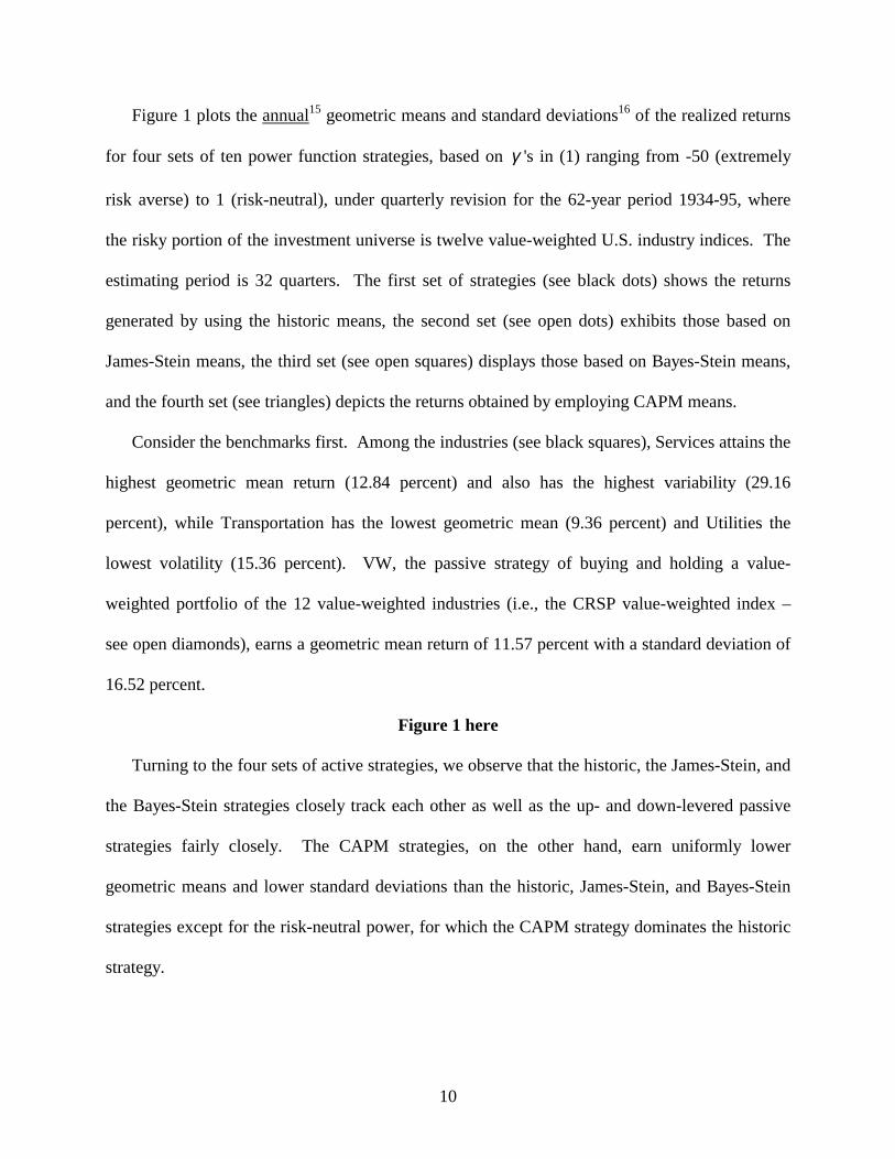
Figure 1 plots the annual15 geometric means and standard deviations16 of the realized returns

for four sets of ten power function strategies, based on γ 's in (1) ranging from -50 (extremely

risk averse) to 1 (risk-neutral), under quarterly revision for the 62-year period 1934-95, where

the risky portion of the investment universe is twelve value-weighted U.S. industry indices. The

estimating period is 32 quarters. The first set of strategies (see black dots) shows the returns

generated by using the historic means, the second set (see open dots) exhibits those based on

James-Stein means, the third set (see open squares) displays those based on Bayes-Stein means,

and the fourth set (see triangles) depicts the returns obtained by employing CAPM means.

Consider the benchmarks first. Among the industries (see black squares), Services attains the

highest geometric mean return (12.84 percent) and also has the highest variability (29.16

percent), while Transportation has the lowest geometric mean (9.36 percent) and Utilities the

lowest volatility (15.36 percent). VW, the passive strategy of buying and holding a value-

weighted portfolio of the 12 value-weighted industries (i.e., the CRSP value-weighted index –

see open diamonds), earns a geometric mean return of 11.57 percent with a standard deviation of

16.52 percent.

Figure 1 here

Turning to the four sets of active strategies, we observe that the historic, the James-Stein, and

the Bayes-Stein strategies closely track each other as well as the up- and down-levered passive

strategies fairly closely. The CAPM strategies, on the other hand, earn uniformly lower

geometric means and lower standard deviations than the historic, James-Stein, and Bayes-Stein

strategies except for the risk-neutral power, for which the CAPM strategy dominates the historic

strategy.

11

Figure 2 plots the corresponding results for the 30-year 1966-1995 sub-period. Among the

industries, Food and Tobacco attain the highest geometric mean return (15.00 percent) and

Leisure experiences the highest volatility (26.53 percent), while Transportation has the lowest

geometric mean (7.81 percent) and Utilities the lowest volatility (13.88 percent). The passive

strategy VW earns 10.67 percent with a volatility of 15.58 percent.

Figure 2 here

Turning to the four sets of active strategies, three features stand out. First, the strategies

based on CAPM means are clearly "dominated" by the other three. Second, the strategies based

on historic, James-Stein, and Bayes-Stein means appear to attain "superior" performance when

compared to the up- and down-levered value-weighted benchmark portfolios – whether this in

fact is the case will be formally addressed in the next section. Third, for each of these three

strategies, the logarithmic utility function (power 0) achieves the highest geometric mean return

(16.69 percent for Bayes-Stein, 14.44 percent for James-Stein, and 14.23 percent for the historic

case) – which is asymptotically the case when the correct probability distribution is used. Since

each point in Figure 2 is based on 120 quarterly portfolio choices, a sizable number of

observations, the suggested interpretation here is that each of the three estimators (historic

EPAA, James-Stein, and Bayes-Stein) are unbiased.

Figure 3 displays the results for the (inflationary) 16-year sub-period 1966-1981. Petroleum

has the highest geometric mean (11.2 percent) and Leisure the highest standard deviation (33.62

percent). Consumer durables experience the lowest geometric mean (4.19 percent) and Utilities

the lowest volatility (13.63 percent). Note that the compound return on the risk-free asset is 6.98

percent per year vs. 6.44 percent for the value-weighted portfolio of all stocks, i.e., the 16-year

period 1966-81 experiences a one half percent per year negative realized risk premium! It is

12

therefore perhaps not surprising that the rear-view approach of the EPAA generates rather

conservative investment portfolios, as is reflected in Table 3.

Figure 3 here

VI. Performance Tests

There are a number of commonly accepted ways of testing for abnormal investment

performance. This study employs Grinblatt and Titman's (1993) portfolio change measure as

well as conditional and unconditional versions of Jensen's test of selectivity and Henriksson and

Merton's and Treynor and Mazuy's market-timing tests. The null hypothesis is that there is no

superior investment performance and the alternative hypothesis is that there is. Thus, we report

the results of one-tailed tests. All regressions are corrected for heteroscedasticity using White's

(1980) correction.

The unconditional Jensen model is

ptmtpppt uRR ++= βα , (12)

where Rpt is the excess return on portfolio p over the Treasury bill rate, Rmt is the excess return

on the CRSP value-weighted index, pα is the unconditional measure of performance, and βp is

the unconditional beta. However, expected returns and betas may change over time. For

example, Fama and French (1988) predict expected returns conditioned on dividend yields.

Therefore, Ferson and Schadt (1996), Ferson and Warther (1996), Harvey and Graham (1995),

and Kryzanowski, Lalancette, and To (1997), building on the earlier work of Shanken (1990),

Ball, Kothari, and Shanken (1995), and Chen and Knez (1996), advocate conditional

performance measures.

In this paper, we follow Ferson and Schadt's (1996) and Ferson and Warther's (1996)

suggestion that a portfolio's risk should be related to market indicators such as dividend yields

13

and short-term Treasury yields lagged one period when assessing performance. We employ the

same variables except that we measure the T-bill yield as of the beginning of the period. Thus,

we postulate that

Ltptppp rbdybb 2110 ++= −β , (13)

where dyt-1 is the CRSP NYSE-AMEX value-weighted index annual dividend yield as of the

beginning of period t and rLt is the (observable) beginning-of-quarter Treasury bill rate, both

measured as deviations from their estimation-period means. Substituting equation (13) into

equation (12), yields the conditional Jensen model

ptmtLtpmttpmtpcppt eRrbRdybRbR ++++= − ][][ 2110α , (14)

where αcp is the conditional measure of performance, b0p is the conditional beta, and b1p and b2p

measure how the conditional beta varies with respect to dividend yields and Treasury bill rates.

The unconditional regression specification for the Treynor-Mazuy model is

ptmtpmtpppt uRRR +++= 2γβα , (15)

where αp is the measure of selectivity, βp is the unconditional beta, and γp is the market-timing

coefficient. Substituting for βp, the conditional regression specification becomes

ptmtpmtLtpmttpmtpcppt eRRrbRdybRbR +++++= −2

2110 ][][ γα , (16)

where αcp, b0p, b1p, b2p, and γp are defined above.

The unconditional Henriksson-Merton model is given by

ptmtpmtdpppt uRRR +++= ),0max(γβα , (17)

where αp is the measure of selectivity, βdp is the down-market beta, γp is the market-timing

coefficient, in this case the difference between the up- and down-market beta, and max(0,Rmt) is

14

the payoff on a call option on the market with exercise price equal to the riskfree rate of interest.

Following Ferson and Schadt (1996), the conditional Henriksson-Merton model is

ptmtLtpmttpmtpmtLtpmttpmtdpcppt eRrbRdybRRrbRdybRbR +++++++= −− ][][][][ **2

*1

*1

*211 γα , (18)

where *mtR is the product of the excess return on the CRSP value-weighted index and an

indicator dummy for positive values of the difference between the excess return on the index and

the conditional mean of the excess return. (The conditional mean is estimated by a linear

regression of the excess return of the CRSP value-weighted index on dyt-1 and rLt.) The most

important coefficients are bdp, the conditional down-market beta, and γp the market-timing

coefficient, which in this case is the difference between the up- and down-market conditional

beta.

In contrast to most other performance measures, Grinblatt and Titman's (1993) portfolio

change measure employs portfolio holdings as well as rates of return. In order to motivate the

portfolio change measure, assume that uninformed investors perceive that the vector of expected

returns is constant, while informed investors can predict whether expected returns vary over

time. Informed investors can profit from changing expected returns by increasing (decreasing)

their holdings of assets whose expected returns have increased (decreased). The holding of an

asset that increases with an increase in its conditional expected rate of return will exhibit a

positive unconditional covariance with the asset's returns. The portfolio change measure is

constructed from an aggregation of these covariances. For evaluation purposes, let

PCMt = ∑ −−i

jtiitit xxr )( , ,

where rit is the quarterly rate of return on asset i time t, xit and xi,t-j are the holdings of asset i at

time t and time t-j, respectively. This expression provides an estimate of the covariance between

15

returns and weights at a point in time. Alternatively, it may be viewed as the return on zero-

weight portfolio. The portfolio change measure is an average of the PCMts

( )[ ]∑∑ −−=t i

jtiitit TxxrMCP /, , (19)

where T is the number of time-series observations. The portfolio change measure test itself is a

simple t-test based on the time series of zero-weight portfolio returns, i.e.,

( )( ) TPCMMCPt σ/= , (20)

where σ(PCM) is the standard deviation of the time series of PCMts. In their empirical analysis

of mutual fund performance, Grinblatt and Titman work with two values of j that represented

one- and four-quarter lags. We employ the same two lags.

The portfolio change measure is particularly apropos in the present study because the

portfolio weights are chosen according to a prespecified set of rules over the same quarterly time

interval as performance is measured. Thus, we do not have to worry about possible gaming or

window dressing problems that face researchers trying to gauge the performance of mutual

funds.

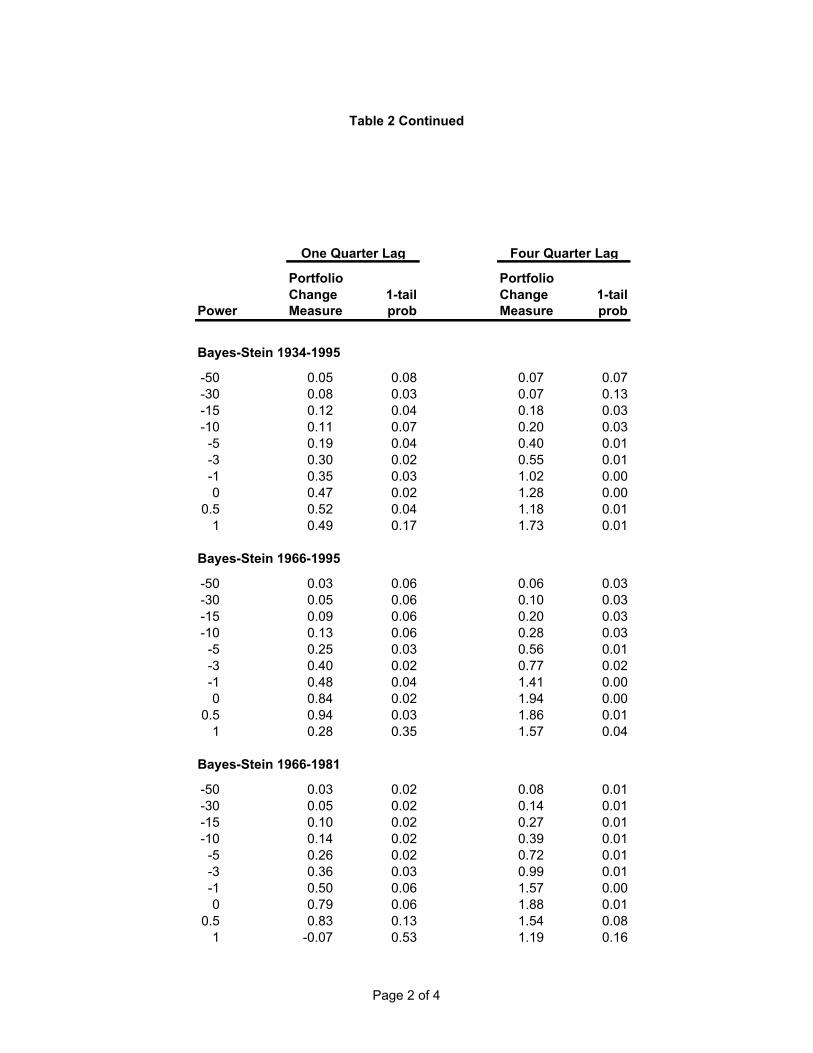
Table 2 shows the results of the Grinblatt-Titman tests with both one-quarter and four-quarter

lags for each of the four mean estimators (historic, Bayes-Stein, James-Stein, and CAPM). Each

test incorporates ten relative risk aversion attitudes ranging from 51 to 0 (corresponding to

powers -50 to 1) for the three periods 1934-95, 1966-95, and 1966-81.

Table 2 here

Several observations strike the reader. First, the test based on a four-quarter lag tends to give

higher marks than the one based on a one-quarter lag, except for the CAPM estimator. Second,

the CAPM estimator receives low scores in all cases except for the very risk-averse powers

during 1966-81 in the one-quarter lag case. Third, excess returns at the 5 percent level of

16

significance are earned by most powers in both the 1966-95 and the 1966-81 sub-periods when

the historic, Bayes-Stein, and James-Stein estimators are employed, while fewer such instances

occur over the full 1934-95 period. These findings are consistent with the overall impression

conveyed by Figures 1, 2 and 3.

Ferson and Khang (2000) show that the portfolio change measure can attribute positive

returns to a strategy that draws on public information to generate weights that are correlated with

conditional expected returns. One possible explanation for our results then is that the 32-quarter

raw joint returns of the estimation period cleverly capture valuable public information. To the

extent that the results are due to a momentum effect, the stronger effect associated with the four-

quarter lag is consistent with the observation that momentum tends to be stronger over 12

months than over periods less than 6 months.

Table 3 shows the quarterly returns and portfolio choices made by the power -5 investor

when the Bayes-Stein estimator is used for the 24 quarters from 1972 through 1977. It is

apparent that the portfolios chosen during this period are quite conservative. Note also that

portfolio changes from quarter to quarter are quite small, implying only modest transaction costs.

Table 3 here

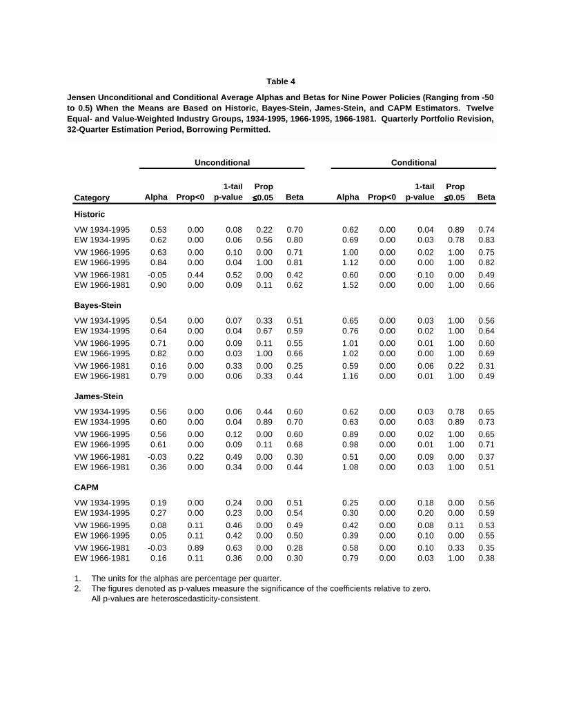
Table 4 summarizes the average alphas and betas for nine powers ranging from -50 to .5

obtained from the conditional and unconditional Jensen tests. The table incorporates each of the

aforementioned four estimators over the same three periods as in Table 2, both when the twelve

industry sectors are value-weighted as well as when they are equal-weighted. The upper part of

Table 7 provides the details for the value-weighted case of the Bayes-Stein estimator over the

1966-95 sub-period.

Table 4 here

17

The most striking aspect of Table 4 is that the conditional test uniformly ranks the various

investors' performance higher than the unconditional one. Based on the conditional Jensen test,

the historic, Bayes-Stein, and James-Stein estimators' excess returns are highly significant in

each period.

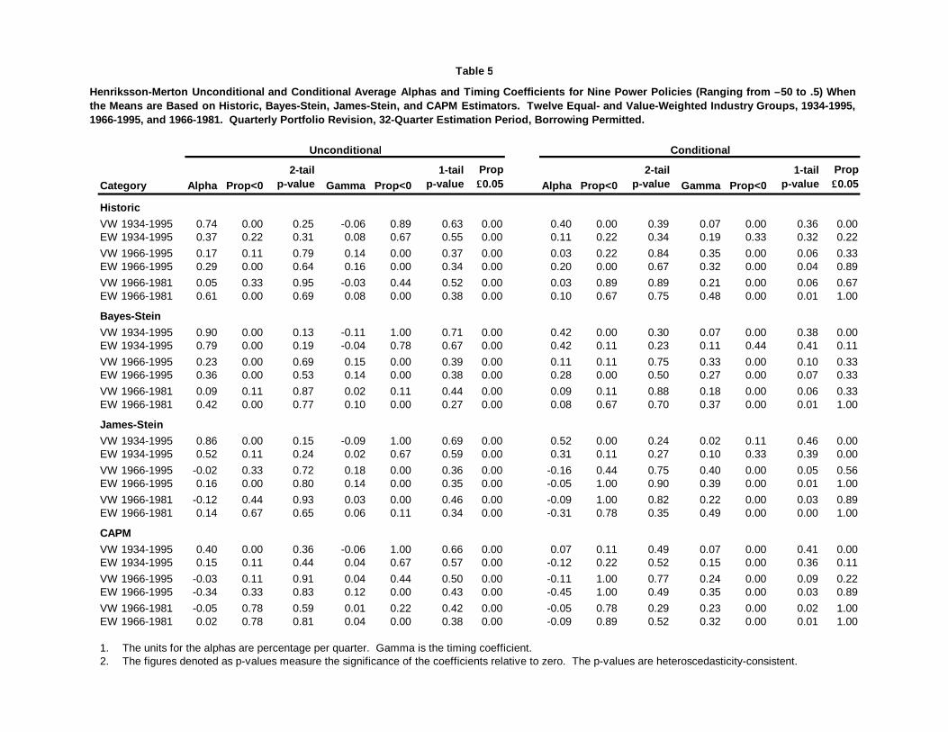
Table 5 reveals that the Henriksson-Merton conditional test also ranks the return sequences

higher than the unconditional one does. However, accolades for excess returns are given by the

conditional Henriksson-Merton test to the historic, Bayes-Stein, and James-Stein estimators only

for the 1966-95 and 1966-81 sub-periods. On the other hand, the Henriksson-Merton conditional

test rates the CAPM estimators' performance in those two periods higher than the corresponding

Jensen test does.

Table 5 here

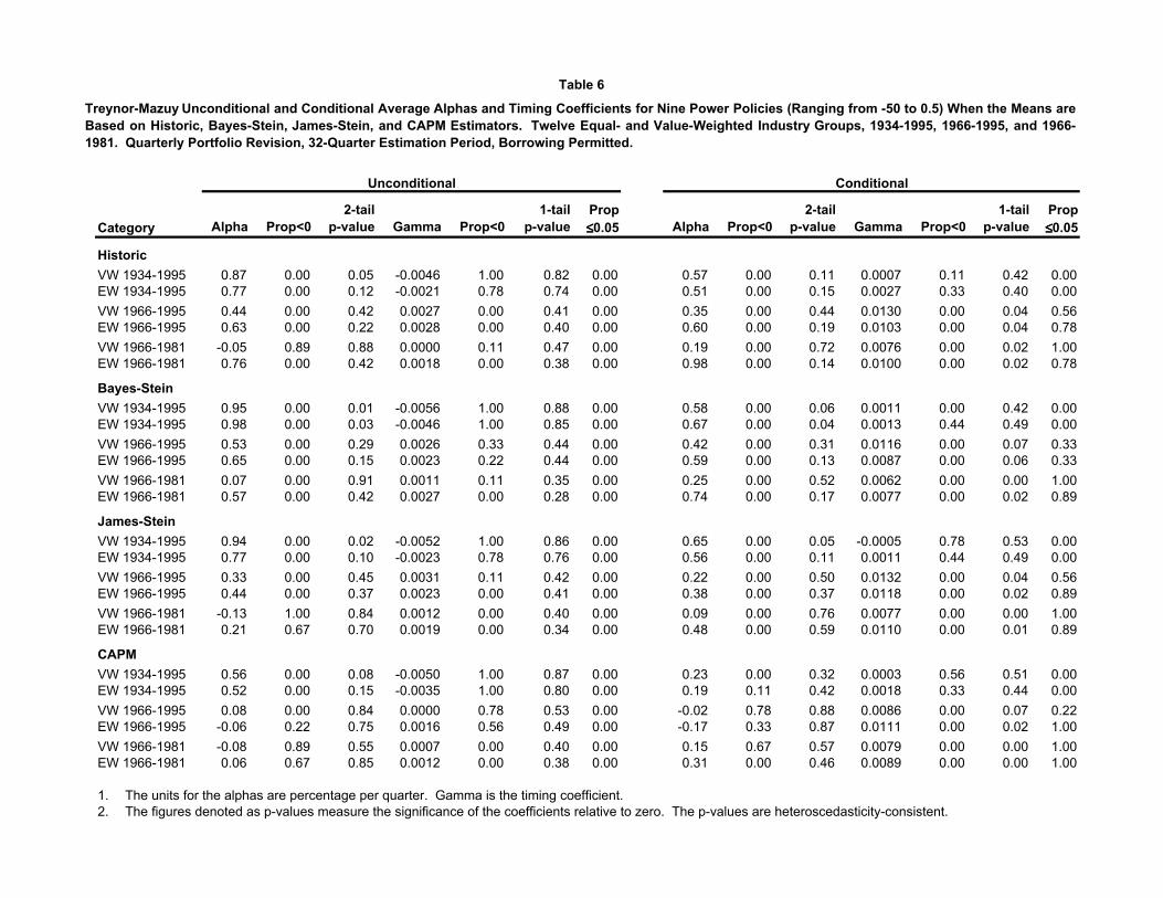
Table 6 summarizes the Treynor-Mazuy unconditional and conditional alphas and timing

coefficients for the same nine powers as in Tables 4 and 5, as well as for the same estimators and

periods and for both the value- and equal-weighted cases. Details for the conditional value-

weighted Bayes-Stein strategies are given in the lower part of Table 7. As in the Jensen and

Henriksson-Merton tests, the conditional test gives higher marks than the unconditional one

(which finds no statistically significant excess returns) across the board. Somewhat surprisingly,

all four estimators achieved superior excess returns over the 1966-95, and especially the 1966-

81, periods according to the Treynor-Mazuy conditional test.

Table 6 here

Table 7 also shows the regression coefficients on the lagged dividend yield (b1) and on

Treasury bill rates (b2). The coefficients on the dividend yield are negative and often significant

while those on Treasury bills are positive. This is consistent with what Ferson and Warther

18

(1996) observed for a buy and hold strategy of a combination of stocks and bonds and for real-

world mutual funds. The results are puzzling, however, as one would expect just the opposite:

positive (negative) signs on the dividend yield (T-bill) coefficients. While Ferson and Wather

present evidence that cash flows into mutual funds partly explain the changes in the mutual-fund

betas, it remains a puzzle why the buy and hold betas, the mutual fund betas, and the power

utility betas all exhibit this unexpected behavior.

Table 7 here

VII. Discussion of Results

Most findings of excess returns are associated with studies of momentum and contrarian

strategies, either at the stock selection level (see e.g. DeBondt and Thaler (1985, 1987),

Lehmann (1990), Jagadeesh (1990), Jagadeesh and Titman (1993)) or at the industry level (see

Moskowitz and Grinblatt (1999)). These studies employ short formation or estimation periods,

typically one month to a year, occasionally as long as five years, and use holding periods of

similar lengths. The returns of the top performers during the formation period (the winners) are

then compared to those of the losers, usually held short, during the holding period. At the stock

selection level, contrarian strategies generally do best over the short run, such as a month, and

over periods longer than two years, while momentum strategies typically outperform over

periods 6 months up to 2 years in length. Industry momentum, however, appears strongest over a

single month and seems to contribute the bulk of the profitability generated by individual stock

selection momentum strategies - see Moskowitz and Grinblatt (1999).

Are the results of the present study due to momentum? If so, it provides several new

findings. First, it adds a 32-quarter formation period/1 quarter holding period to the literature, a

rather significant departure from earlier studies. Second, it uses an investment model to pick its

19

portfolio rather than selecting previous winners and losers, a feature which clearly appears to

ameliorate against finding excess returns. Third, the findings are robust across a very wide range

of stationary risk attitudes. Finally, no short positions are involved, which would seemingly

reduce the chances for positive measures. What the study suggests, then, is that the (complete)

moment-comoment structure of the empirical probability assessment approach contains valuable

information beyond dividend yields and short-term interest rates that the dynamic investment

model is able to profitably exploit.

VIII. Summary

This paper applies Grinblatt and Titman's portfolio change measure, with one- and four-

quarter lags, and conditional selectivity and market-timing measures to assess the performance of

the dynamic investment model in various industry-rotation settings spanning the 1934-1995

period. The dynamic investment model used in the study employs the empirical probability

assessment approach with a 32-quarter rear-view-moving window; both in raw form and with

adjustments for estimation error based on a James-Stein, a Bayes-Stein, and a CAPM-based

correction. Portfolio choices are implemented for a wide range of risk attitudes.

The verdicts of the various tests are remarkably unanimous. The portfolio change measure

and the conditional Jensen, Henriksson-Merton, and Treynor-Mazuy tests come to the conclusion

that the excess returns attained by the (unadjusted) historic, the Bayes-Stein, and the James-Stein

estimators are (in some cases highly) statistically significant over the 1966-95 and 1966-81 sub-

periods. Only the conditional Jensen test rates the full 1934-95 performance superior. The

CAPM estimator, on the other hand, performs poorly except in the eyes of the conditional

Treynor-Mazuy test over the 1966-95 and 1981-95 sub-periods. This evidence suggests that the

empirical probability assessment approach based on the recent past, with and without Stein-

20

based corrections for estimation error, contains information beyond dividend yields and short-

term interest rates embedded in its moment-comoment structure that can be profitably exploited.

21

References

Balduzzi, P., and A. W. Lynch, 1999, Transaction costs and predictability: some utility cost calculations, Journal of Financial Economics 52, 47-78.

Ball, R., S. P. Kothari, and J. Shanken, 1995, Problems in measuring portfolio performance: An application to investment strategies, Journal of Financial Economics 38, 79-107.

Barberis, N., 2000, Investing for the long run when returns are predictable, Journal of Finance 55, 225-264.

Best, M. J., 1975, A feasible conjugate direction method to solve linearly constrained optimization problems, Journal of Optimization Theory and Applications 16, 25-38.

Best, M. J., and R. R. Grauer, 1991, On the sensitivity of mean-variance-efficient portfolios to changes in asset means: some analytical and computational results, Review of Financial Studies 4, 315-342.

Campbell, J. Y., and Viceira, L. M., 1999, Consumption and portfolio decisions when expected returns are time varying, Quarterly Journal of Economics 114, 433-495.

Chen Z., and P. Knez, 1996, Portfolio performance measurement: Theory and applications, Review of Financial Studies 9, 511-556.

Cheng, P. L., and R. R. Grauer, 1980, An alternative test of the capital asset pricing model, American Economic Review 70, 660-671.

DeBondt, W. F. M., and R. Thaler, 1985, Does the stock market overreact? Journal of Finance 40, 793-805.

DeBondt, W. F. M., and R. Thaler, 1987, Further evidence on investor overreaction and stock market seasonality, Journal of Finance 42, 557-581.

Efron, B., and C. Morris, 1973, Stein's estimation rule and its competitors--An empirical Bayes approach, Journal of the American Statistical Association 68, 117-130.

Efron, B., and C. Morris, 1975, Data analysis using Stein's estimator and its generalizations, Journal of the American Statistical Association 70, 311-319.

Efron, B., and C. Morris, 1977, Stein's paradox in statistics, Scientific American 236, 119-127.

Fama, E., and K. French, 1988, Dividend yields and expected stock returns, Journal of Financial Economics 22, 3-25.

Ferson, W. E., and R. W. Schadt, 1996, Measuring fund strategy and performance in changing economic conditions, Journal of Finance 51, 425-462.

Ferson, W. E., and V. A. Warther, 1996, Evaluating fund performance in a dynamic market, Financial Analysts Journal 52, 20-28.

Ferson, W. E., and K. Khang, 2000, Conditional performance measurement using portfolio weights: Evidence for pension funds, manuscript University of Washington.

Grauer, R. R., 1991, Further ambiguity when performance is measured by the security market line, Financial Review 26, 569-585.

22

Grauer, R. R., and N. H. Hakansson, 1986, A half century of returns on levered and unlevered portfolios of stocks, bonds, and bills, with and without small stocks, Journal of Business 59, 287-318.

Grauer, R. R., and N. H. Hakansson, 1987, Gains from international diversification: 1968-85 returns on portfolios of stocks and bonds, Journal of Finance 42, 721-739.

Grauer, R. R., and N. H. Hakansson, 1995a, Gains from diversifying into real estate: Three decades of portfolio returns based on the dynamic investment model, Real Estate Economics 23, 117-159.

Grauer, R. R., and N. H. Hakansson, 1995b, Stein and CAPM estimators of the means in asset allocation, International Review of Financial Analysis 4, 35-66.

Grauer, R. R., and N. H. Hakansson, 1998, On timing the market: The empirical probability assessment approach with an inflation adapter, in John Mulvey and William Ziemba, Eds. Worldwide Asset and Liability Modeling Cambridge University Press, 149-181.

Grauer, R. R., N. H. Hakansson, and F. C. Shen, 1990, Industry rotation in the U.S. stock market: 1934-1986 returns on passive, semi-passive, and active strategies, Journal of Banking and Finance 14, 513-535.

Grauer, R. R., and F. C. Shen, 1998, On estimation risk and discrete-time dynamic portfolio theory: the evidence from asset allocation, manuscript Simon Fraser University.

Grauer, R. R., and F. C. Shen, 2000, Do constraints improve portfolio performance? Journal of Banking and Finance 24, 1253-1274.

Grinblatt, M., and S. Titman, 1993, Performance measurement without benchmarks: an examination of mutual fund returns, Journal of Business 66, 47-68.

Hakansson, N. H., 1974, Convergence to isoelastic utility and policy in multiperiod portfolio choice, Journal of Financial Economics 1, 201-224.

Harvey, C., and Graham, J., 1996, Market timing ability and volatility implied in investment newsletter asset allocation recommendations, Journal of Financial Economics 42, 397-421.

Henriksson, R. D., and R. C. Merton, 1981, On market timing and investment performance. II. Statistical procedures for evaluation forecasting skills, Journal of Business 54, 513-533.

Huberman, G., and S. Ross, 1983, Portfolio turnpike theorems, risk aversion and regularly varying utility functions, Econometrica 51, 1104-1119.

Jagadeesh, N., 1990, Evidence of predictable behavior in security returns, Journal of Finance 45, 881-898.

Jagadeesh, N., and S. Titman, 1993, Returns to buying winners and selling losers: Implications for stock market efficiency, Journal of Finance 48, 65-91.

James, W., and C. Stein, 1961, Estimation with quadratic loss, Proceedings of the 4th Berkeley Symposium on Probability and Statistics I, University of California Press, Berkeley, 361-379.

Jensen, M. C., 1968, The performance of mutual funds in the period 1945-1964, Journal of Finance 23, 389-416.

23

Jobson, J. D., and B. Korkie, 1980, Estimation for Markowitz efficient portfolios, Journal of the American Statistical Association 75, 544-554.

Jobson, J. D., and B. Korkie, 1981, Putting Markowitz theory to work, Journal of Portfolio Management 7, 70-74.

Jobson, J. D., B. Korkie, and V. Ratti, 1979, Improved estimation for Markowitz portfolios using James-Stein type estimators, Proceedings of the American Statistical Association, Business and Economics Statistics Section 41, 279-284.

Jorion, P., 1985, International portfolio diversification with estimation risk, Journal of Business 58, 259-278.

Jorion, P., 1986, Bayes-Stein estimation for portfolio analysis, Journal of Financial and Quantitative Analysis 21, 279-292.

Jorion, P., 1991, Bayesian and CAPM estimators of the means: implications for portfolio selection, Journal of Banking and Finance 15, 717-727.

Kandel, S., and R. Stambaugh, 1996, On the predictability of stock returns: An asset allocation perspective, Journal of Finance 51, 385-424.

Kim, T. S., and E. Omberg, 1996, Dynamic nonmyopic portfolio behavior, Review of Financial Studies 9, 141-161,

Kryzanowski, L., Lalancette, S., and M. To, 1997, Performance attribution using an APT with prespecified macrofactors and time-varying risk premia and betas, Journal of Financial and Quantitative Analysis 32, 205-224.

Leland, H., 1972, On turnpike portfolios, in K. Shell and G. P. Szego, Eds. Mathematical Methods in Investment and Finance, North-Holland, Amsterdam.

Lehmann, B., 1990, Fads, martingales, and market efficiency, Quarterly Journal of Economics 105, 1-28.

Lintner, J., 1965, The valuation of risk assets and the selection of risky investments in stock portfolios and capital budgets, Review of Economics and Statistics 47, 13-47.

Moskowitz, J., and M. Grinblatt, 1999, Do industries explain momentum?, The Journal of Finance 54, 1249-1290. Roll, R., 1978, Ambiguity when performance is measured by the securities market line, Journal of Finance 33, 1051-1069.

Shanken, J., 1990, Intertemporal asset pricing: an empirical investigation, Journal of Econometrics 45, 99-120.

Sharpe, W. F. 1964, Capital asset prices: A theory of market equilibrium under conditions of risk, Journal of Finance 19, 101-121.

Stein, C., 1955, Inadmissibility of the usual estimator for the mean of a multivariate normal distribution, Proceedings of the 3rd Berkeley Symposium on Probability and Statistics I, University of California Press, Berkeley, 197-206.

Treynor, J. L., and K. Mazuy, 1966, Can mutual funds outguess the market? Harvard Business Review 44, 131-136.

24

White, H., 1980, A heteroscedasticity-consistent covariance matrix estimator and a direct test for heteroscedasticity, Econometrica 48, 817-838.

25

Footnotes

1 Grauer and Shen (1998, 2000) explore additional ways of allowing for estimation risk. The first paper investigates nine alternative ways of estimating the joint return distribution. The second examines whether constraints improve performance. 2 The simple reinvestment formulation does ignore consumption of course. For more elaborate models with and without consumption, see e.g. Kim and Omberg (1996), Kandel and Stambaugh (1996), Barberis (2000), Balduzzi and Lynch (1999), and Campbell and Viceira (1999). 3 By convention, all vectors in this paper are column vectors and a prime indicates transposition. 4 The solvency constraint (6) is not binding for the power functions with 1<γ and discrete probability distributions with a finite number of outcomes because the marginal utility of zero wealth is infinite. Nonetheless, it is convenient to explicitly consider (6) so that the nonlinear programming algorithm used to solve the investment problems does not attempt to evaluate an infeasible policy as it searches for the optimum. 5 The nonlinear programming algorithm employed is described in Best (1975). 6 The realized borrowing rate is calculated as a monthly average. 7 Note that if k = 32 under quarterly revision, then the first quarter for which a portfolio can be selected is b+32, where b is the first quarter for which data is available. 8 See Jobson, Korkie, and Ratti (1979), Jobson and Korkie (1980, 1981), and Jorion (1985, 1986, 1991). 9 For discussion of James-Stein estimators, see Efron and Morris (1973, 1975, and 1977). 10 As Jorion has noted, this conclusion is difficult to reconcile with the generally accepted trade-off between risk and expected return, unless all stocks fall within the same risk class. 11 Having calculated the James-Stein and historic means for asset i, we add the difference

)( itJSit rr − , where JSitr and itr are the James-Stein and historic means for asset i at time t, to each actual return on asset i in the estimation period. That is, in each estimation period, we replace the raw return series with the adjusted return series

),( itJSitiA

i rrrr −+= ττ for all i and τ .

Thus, the mean vector of the adjusted series is equal to the James-Stein means of the original series; all other moments are unchanged. 12 We do not assume, however, that the CAPM holds. Both the market portfolio and β exist independently of the CAPM. What this estimator tries to capture, then, is the observation, well

26

documented in most countries, that over intermediate to long periods, realized average returns on financial assets are an increasing function of systematic risk. 13 At this point, we proceed as in the James-Stein and Bayes-Stein means-cases, adding the difference between the CAPM means and the historic means to the actual returns in the estimation period. Consequently, the mean vector of the adjusted series is equal to the CAPM means; all other moments are unchanged. 14 There was no practical way to take maintenance margins into account in our programs. In any case, it is evident from the results that they would come into play only for the more risk-tolerant strategies, and even for them only occasionally, and that the net effect would be relatively neutral. 15 Annual returns were obtained by compounding the quarterly realized returns. 16 For consistency with the geometric mean, the standard deviation is based on the log of one plus the rate of return. This quantity is very similar to the standard deviation of the rate of return for levels less than 25 percent.

Table 1

Asset Category and Fixed-Weight Portfolio Symbols

PETR Petroleum RL Riskfree Lending

FINA Finance and Real Estate B Borrowing

CDUR Consumer Durables VW Value-Weighted Portfolio of Risky

BASI Basic Industries Assets

FOOD Food and Tobacco V5 50% in VW, 50% in RL

CONS Construction V15 150% in VW, 50% in B

CAPG Capital Goods V20 200% in VW, 100% in B

TRAN Transportation

UTIL Utilities

TEXT Textiles and Trade

SERV Services

LEIS Leisure

Portfolio PortfolioChange 1-tail Change 1-tail

Power Measure prob Measure prob

Historic 1934-1995

-50 0.05 0.06 0.10 0.03-30 0.08 0.02 0.11 0.05-15 0.13 0.04 0.24 0.01-10 0.14 0.06 0.33 0.01-5 0.25 0.03 0.56 0.00-3 0.24 0.07 0.75 0.00-1 0.26 0.10 1.02 0.000 0.36 0.11 1.45 0.00

0.5 0.46 0.11 1.26 0.031 0.35 0.25 1.32 0.03

Historic 1966-1995

-50 0.04 0.03 0.08 0.03-30 0.06 0.03 0.13 0.03-15 0.12 0.03 0.25 0.03-10 0.17 0.03 0.37 0.03-5 0.34 0.02 0.68 0.01-3 0.36 0.06 0.95 0.02-1 0.43 0.07 1.13 0.030 0.55 0.11 1.56 0.02

0.5 0.94 0.03 1.62 0.031 -0.01 0.51 0.73 0.17

Historic 1966-1981

-50 0.04 0.02 0.08 0.03-30 0.06 0.02 0.13 0.03-15 0.12 0.02 0.26 0.03-10 0.18 0.02 0.38 0.03-5 0.32 0.02 0.69 0.03-3 0.37 0.04 0.77 0.06-1 0.32 0.18 0.69 0.170 0.32 0.30 0.95 0.20

0.5 1.12 0.07 1.52 0.141 -0.49 0.67 0.09 0.47

Table 2

One Quarter Lag Four Quarter Lag

Grinblatt-Titman Portfolio Change Measures Based on One Quarterand Four Quarter Lags for the Power Policies When the Means areBased on Historic, Bayes-Stein, James-Stein, and CAPM Estimators.Twelve Value-Weighted Industry Groups, 1934-1995, 1966-1995, 1966-1981. Quarterly Portfolio Revision, 32 Quarter Estimation Period,Borrowing Permitted.

Page 1 of 4

Portfolio PortfolioChange 1-tail Change 1-tail

Power Measure prob Measure prob

Bayes-Stein 1934-1995

-50 0.05 0.08 0.07 0.07-30 0.08 0.03 0.07 0.13-15 0.12 0.04 0.18 0.03-10 0.11 0.07 0.20 0.03-5 0.19 0.04 0.40 0.01-3 0.30 0.02 0.55 0.01-1 0.35 0.03 1.02 0.000 0.47 0.02 1.28 0.00

0.5 0.52 0.04 1.18 0.011 0.49 0.17 1.73 0.01

Bayes-Stein 1966-1995

-50 0.03 0.06 0.06 0.03-30 0.05 0.06 0.10 0.03-15 0.09 0.06 0.20 0.03-10 0.13 0.06 0.28 0.03-5 0.25 0.03 0.56 0.01-3 0.40 0.02 0.77 0.02-1 0.48 0.04 1.41 0.000 0.84 0.02 1.94 0.00

0.5 0.94 0.03 1.86 0.011 0.28 0.35 1.57 0.04

Bayes-Stein 1966-1981

-50 0.03 0.02 0.08 0.01-30 0.05 0.02 0.14 0.01-15 0.10 0.02 0.27 0.01-10 0.14 0.02 0.39 0.01-5 0.26 0.02 0.72 0.01-3 0.36 0.03 0.99 0.01-1 0.50 0.06 1.57 0.000 0.79 0.06 1.88 0.01

0.5 0.83 0.13 1.54 0.081 -0.07 0.53 1.19 0.16

One Quarter Lag Four Quarter Lag

Table 2 Continued

Page 2 of 4

Portfolio PortfolioChange 1-tail Change 1-tail

Power Measure prob Measure prob

James-Stein 1934-1995

-50 0.06 0.04 0.06 0.11-30 0.08 0.02 0.05 0.20-15 0.13 0.04 0.15 0.06-10 0.14 0.04 0.21 0.04-5 0.28 0.01 0.43 0.01-3 0.38 0.01 0.56 0.01-1 0.43 0.01 0.89 0.000 0.27 0.15 1.09 0.01

0.5 0.47 0.06 1.19 0.021 0.68 0.05 1.93 0.00

James-Stein 1966-1995

-50 0.04 0.02 0.06 0.05-30 0.07 0.02 0.10 0.05-15 0.13 0.02 0.19 0.05-10 0.17 0.02 0.27 0.05-5 0.37 0.01 0.58 0.02-3 0.47 0.01 0.68 0.04-1 0.58 0.03 1.15 0.020 0.56 0.10 1.76 0.02

0.5 0.87 0.04 1.66 0.031 0.58 0.19 1.94 0.03

James-Stein 1966-1981

-50 0.05 0.00 0.09 0.02-30 0.08 0.00 0.14 0.02-15 0.15 0.00 0.28 0.02-10 0.22 0.00 0.40 0.02-5 0.40 0.00 0.74 0.02-3 0.49 0.01 0.85 0.03-1 0.53 0.04 1.39 0.010 0.48 0.15 1.48 0.08

0.5 0.79 0.14 1.08 0.201 0.51 0.31 1.50 0.15

Table 2 Continued

One Quarter Lag Four Quarter Lag

Page 3 of 4

Portfolio PortfolioChange 1-tail Change 1-tail

Power Measure prob Measure prob

CAPM 1934-1995

-50 0.01 0.19 -0.03 0.85-30 0.02 0.19 -0.05 0.85-15 0.05 0.14 -0.04 0.69-10 0.07 0.10 -0.09 0.83-5 0.08 0.12 -0.07 0.72-3 0.05 0.30 -0.1 0.73-1 -0.02 0.57 -0.18 0.790 0.15 0.20 -0.17 0.68

0.5 0.16 0.25 0.33 0.231 0.47 0.07 1.08 0.03

CAPM 1966-1995

-50 0.01 0.11 0.01 0.37-30 0.02 0.11 0.01 0.37-15 0.03 0.11 0.02 0.37-10 0.05 0.10 0.03 0.37-5 0.09 0.10 0.05 0.36-3 0.14 0.10 0.08 0.36-1 0.22 0.13 0.26 0.230 0.39 0.09 0.20 0.37

0.5 0.48 0.09 0.92 0.081 0.83 0.01 1.38 0.02

CAPM 1966-1981

-50 0.01 0.03 0.01 0.27-30 0.02 0.03 0.02 0.27-15 0.03 0.03 0.04 0.27-10 0.05 0.03 0.06 0.27-5 0.10 0.02 0.11 0.27-3 0.14 0.02 0.16 0.26-1 0.14 0.13 0.09 0.410 0.24 0.17 0.40 0.28

0.5 0.42 0.11 0.58 0.221 1.23 0.03 1.94 0.07

Table 2 Continued

One Quarter Lag Four Quarter Lag

Page 4 of 4

Quarter Return Lending Petroleum Basic FoodCapitalGoods Utilities Textiles Leisure

1972-1 4.45 0.35 0.05 0.33 0.10 0.161972-2 1.26 0.43 0.22 0.17 0.191972-3 0.86 0.48 0.22 0.28 0.021972-4 1.71 0.61 0.01 0.01 0.361973-1 -0.82 0.57 0.11 0.321973-2 -0.54 0.72 0.01 0.271973-3 1.43 0.85 0.151973-4 -0.32 0.87 0.10 0.031974-1 1.94 1.001974-2 2.06 1.001974-3 1.94 1.001974-4 1.81 1.001975-1 1.62 1.001975-2 1.94 0.95 0.051975-3 0.62 0.89 0.09 0.021975-4 1.52 1.001976-1 1.47 0.95 0.051976-2 1.73 0.86 0.04 0.04 0.061976-3 1.44 0.98 0.011976-4 1.26 0.991977-1 0.78 0.94 0.01 0.01 0.041977-2 1.27 0.97 0.01 0.01 0.021977-3 0.89 0.91 0.02 0.02 0.051977-4 1.43 0.96 0.01 0.01 0.02

1. The units of the returns are percentage per quarter. 2. The portfolio weights are reported as decimal fractions. Except for rounding, the fractions in

a quarter sum to one.3. Borrowing, Finance and Real Estate, Consumer Durables, Construction, Transportation,

and Services were not chosen in this time period.

Table 3

Portfolio Weights

Quarterly Returns and Optimal Portfolio Choices for Power -5 When the Means are Based onJames-Stein Estimators. Twelve Value-Weighted Industry Groups, 1972-1977. QuarterlyPortfolio Revision, 32-Quarter Estimation Period, Borrowing Permitted.

Category Alpha Prop<01-tail

p-valueProp≤≤≤≤0.05 Beta Alpha Prop<0

1-tailp-value

Prop≤≤≤≤0.05 Beta

Historic

VW 1934-1995 0.53 0.00 0.08 0.22 0.70 0.00 0.62 0.00 0.04 0.89 0.74EW 1934-1995 0.62 0.00 0.06 0.56 0.80 0.00 0.69 0.00 0.03 0.78 0.83VW 1966-1995 0.63 0.00 0.10 0.00 0.71 0.00 1.00 0.00 0.02 1.00 0.75EW 1966-1995 0.84 0.00 0.04 1.00 0.81 0.00 1.12 0.00 0.00 1.00 0.82VW 1966-1981 -0.05 0.44 0.52 0.00 0.42 0.00 0.60 0.00 0.10 0.00 0.49EW 1966-1981 0.90 0.00 0.09 0.11 0.62 0.00 1.52 0.00 0.00 1.00 0.66

Bayes-Stein

VW 1934-1995 0.54 0.00 0.07 0.33 0.51 0.00 0.65 0.00 0.03 1.00 0.56EW 1934-1995 0.64 0.00 0.04 0.67 0.59 0.00 0.76 0.00 0.02 1.00 0.64VW 1966-1995 0.71 0.00 0.09 0.11 0.55 0.00 1.01 0.00 0.01 1.00 0.60EW 1966-1995 0.82 0.00 0.03 1.00 0.66 0.00 1.02 0.00 0.00 1.00 0.69VW 1966-1981 0.16 0.00 0.33 0.00 0.25 0.00 0.59 0.00 0.06 0.22 0.31EW 1966-1981 0.79 0.00 0.06 0.33 0.44 0.00 1.16 0.00 0.01 1.00 0.49

James-Stein

VW 1934-1995 0.56 0.00 0.06 0.44 0.60 0.00 0.62 0.00 0.03 0.78 0.65EW 1934-1995 0.60 0.00 0.04 0.89 0.70 0.00 0.63 0.00 0.03 0.89 0.73VW 1966-1995 0.56 0.00 0.12 0.00 0.60 0.00 0.89 0.00 0.02 1.00 0.65EW 1966-1995 0.61 0.00 0.09 0.11 0.68 0.00 0.98 0.00 0.01 1.00 0.71VW 1966-1981 -0.03 0.22 0.49 0.00 0.30 0.00 0.51 0.00 0.09 0.00 0.37EW 1966-1981 0.36 0.00 0.34 0.00 0.44 0.00 1.08 0.00 0.03 1.00 0.51

CAPM

VW 1934-1995 0.19 0.00 0.24 0.00 0.51 0.00 0.25 0.00 0.18 0.00 0.56EW 1934-1995 0.27 0.00 0.23 0.00 0.54 0.00 0.30 0.00 0.20 0.00 0.59VW 1966-1995 0.08 0.11 0.46 0.00 0.49 0.00 0.42 0.00 0.08 0.11 0.53EW 1966-1995 0.05 0.11 0.42 0.00 0.50 0.00 0.39 0.00 0.10 0.00 0.55VW 1966-1981 -0.03 0.89 0.63 0.00 0.28 0.00 0.58 0.00 0.10 0.33 0.35EW 1966-1981 0.16 0.11 0.36 0.00 0.30 0.00 0.79 0.00 0.03 1.00 0.38

1. The units for the alphas are percentage per quarter.2. The figures denoted as p-values measure the significance of the coefficients relative to zero.

All p-values are heteroscedasticity-consistent.

Unconditional Conditional

Table 4

Jensen Unconditional and Conditional Average Alphas and Betas for Nine Power Policies (Ranging from -50to 0.5) When the Means are Based on Historic, Bayes-Stein, James-Stein, and CAPM Estimators. TwelveEqual- and Value-Weighted Industry Groups, 1934-1995, 1966-1995, 1966-1981. Quarterly Portfolio Revision,32-Quarter Estimation Period, Borrowing Permitted.

Category Alpha Prop<02-tail

p-value Gamma Prop<01-tail

p-valueProp≤0.05 Alpha Prop<0

2-tailp-value Gamma Prop<0

1-tailp-value

Prop≤0.05

HistoricVW 1934-1995 0.74 0.00 0.25 -0.06 0.89 0.63 0.00 0.00 0.40 0.00 0.39 0.07 0.00 0.36 0.00EW 1934-1995 0.37 0.22 0.31 0.08 0.67 0.55 0.00 0.00 0.11 0.22 0.34 0.19 0.33 0.32 0.22VW 1966-1995 0.17 0.11 0.79 0.14 0.00 0.37 0.00 0.00 0.03 0.22 0.84 0.35 0.00 0.06 0.33EW 1966-1995 0.29 0.00 0.64 0.16 0.00 0.34 0.00 0.00 0.20 0.00 0.67 0.32 0.00 0.04 0.89VW 1966-1981 0.05 0.33 0.95 -0.03 0.44 0.52 0.00 0.00 0.03 0.89 0.89 0.21 0.00 0.06 0.67EW 1966-1981 0.61 0.00 0.69 0.08 0.00 0.38 0.00 0.00 0.10 0.67 0.75 0.48 0.00 0.01 1.00

Bayes-SteinVW 1934-1995 0.90 0.00 0.13 -0.11 1.00 0.71 0.00 0.00 0.42 0.00 0.30 0.07 0.00 0.38 0.00EW 1934-1995 0.79 0.00 0.19 -0.04 0.78 0.67 0.00 0.00 0.42 0.11 0.23 0.11 0.44 0.41 0.11VW 1966-1995 0.23 0.00 0.69 0.15 0.00 0.39 0.00 0.00 0.11 0.11 0.75 0.33 0.00 0.10 0.33EW 1966-1995 0.36 0.00 0.53 0.14 0.00 0.38 0.00 0.00 0.28 0.00 0.50 0.27 0.00 0.07 0.33VW 1966-1981 0.09 0.11 0.87 0.02 0.11 0.44 0.00 0.00 0.09 0.11 0.88 0.18 0.00 0.06 0.33EW 1966-1981 0.42 0.00 0.77 0.10 0.00 0.27 0.00 0.00 0.08 0.67 0.70 0.37 0.00 0.01 1.00

James-SteinVW 1934-1995 0.86 0.00 0.15 -0.09 1.00 0.69 0.00 0.00 0.52 0.00 0.24 0.02 0.11 0.46 0.00EW 1934-1995 0.52 0.11 0.24 0.02 0.67 0.59 0.00 0.00 0.31 0.11 0.27 0.10 0.33 0.39 0.00VW 1966-1995 -0.02 0.33 0.72 0.18 0.00 0.36 0.00 0.00 -0.16 0.44 0.75 0.40 0.00 0.05 0.56EW 1966-1995 0.16 0.00 0.80 0.14 0.00 0.35 0.00 0.00 -0.05 1.00 0.90 0.39 0.00 0.01 1.00VW 1966-1981 -0.12 0.44 0.93 0.03 0.00 0.46 0.00 0.00 -0.09 1.00 0.82 0.22 0.00 0.03 0.89EW 1966-1981 0.14 0.67 0.65 0.06 0.11 0.34 0.00 0.00 -0.31 0.78 0.35 0.49 0.00 0.00 1.00

CAPMVW 1934-1995 0.40 0.00 0.36 -0.06 1.00 0.66 0.00 0.00 0.07 0.11 0.49 0.07 0.00 0.41 0.00EW 1934-1995 0.15 0.11 0.44 0.04 0.67 0.57 0.00 0.00 -0.12 0.22 0.52 0.15 0.00 0.36 0.11VW 1966-1995 -0.03 0.11 0.91 0.04 0.44 0.50 0.00 0.00 -0.11 1.00 0.77 0.24 0.00 0.09 0.22EW 1966-1995 -0.34 0.33 0.83 0.12 0.00 0.43 0.00 0.00 -0.45 1.00 0.49 0.35 0.00 0.03 0.89VW 1966-1981 -0.05 0.78 0.59 0.01 0.22 0.42 0.00 0.00 -0.05 0.78 0.29 0.23 0.00 0.02 1.00EW 1966-1981 0.02 0.78 0.81 0.04 0.00 0.38 0.00 0.00 -0.09 0.89 0.52 0.32 0.00 0.01 1.00

1. The units for the alphas are percentage per quarter. Gamma is the timing coefficient.2. The figures denoted as p-values measure the significance of the coefficients relative to zero. The p-values are heteroscedasticity-consistent.

ConditionalUnconditional

Table 5

Henriksson-Merton Unconditional and Conditional Average Alphas and Timing Coefficients for Nine Power Policies (Ranging from –50 to .5) Whenthe Means are Based on Historic, Bayes-Stein, James-Stein, and CAPM Estimators. Twelve Equal- and Value-Weighted Industry Groups, 1934-1995,1966-1995, and 1966-1981. Quarterly Portfolio Revision, 32-Quarter Estimation Period, Borrowing Permitted.

Category Alpha Prop<02-tail

p-value Gamma Prop<01-tail

p-valueProp≤≤≤≤0.05 Alpha Prop<0

2-tailp-value Gamma Prop<0

1-tailp-value

Prop≤≤≤≤0.05

HistoricVW 1934-1995 0.87 0.00 0.05 -0.0046 1.00 0.82 0.00 0.00 0.57 0.00 0.11 0.0007 0.11 0.42 0.00EW 1934-1995 0.77 0.00 0.12 -0.0021 0.78 0.74 0.00 0.00 0.51 0.00 0.15 0.0027 0.33 0.40 0.00VW 1966-1995 0.44 0.00 0.42 0.0027 0.00 0.41 0.00 0.00 0.35 0.00 0.44 0.0130 0.00 0.04 0.56EW 1966-1995 0.63 0.00 0.22 0.0028 0.00 0.40 0.00 0.00 0.60 0.00 0.19 0.0103 0.00 0.04 0.78VW 1966-1981 -0.05 0.89 0.88 0.0000 0.11 0.47 0.00 0.00 0.19 0.00 0.72 0.0076 0.00 0.02 1.00EW 1966-1981 0.76 0.00 0.42 0.0018 0.00 0.38 0.00 0.00 0.98 0.00 0.14 0.0100 0.00 0.02 0.78

Bayes-SteinVW 1934-1995 0.95 0.00 0.01 -0.0056 1.00 0.88 0.00 0.00 0.58 0.00 0.06 0.0011 0.00 0.42 0.00EW 1934-1995 0.98 0.00 0.03 -0.0046 1.00 0.85 0.00 0.00 0.67 0.00 0.04 0.0013 0.44 0.49 0.00VW 1966-1995 0.53 0.00 0.29 0.0026 0.33 0.44 0.00 0.00 0.42 0.00 0.31 0.0116 0.00 0.07 0.33EW 1966-1995 0.65 0.00 0.15 0.0023 0.22 0.44 0.00 0.00 0.59 0.00 0.13 0.0087 0.00 0.06 0.33VW 1966-1981 0.07 0.00 0.91 0.0011 0.11 0.35 0.00 0.00 0.25 0.00 0.52 0.0062 0.00 0.00 1.00EW 1966-1981 0.57 0.00 0.42 0.0027 0.00 0.28 0.00 0.00 0.74 0.00 0.17 0.0077 0.00 0.02 0.89

James-SteinVW 1934-1995 0.94 0.00 0.02 -0.0052 1.00 0.86 0.00 0.00 0.65 0.00 0.05 -0.0005 0.78 0.53 0.00EW 1934-1995 0.77 0.00 0.10 -0.0023 0.78 0.76 0.00 0.00 0.56 0.00 0.11 0.0011 0.44 0.49 0.00VW 1966-1995 0.33 0.00 0.45 0.0031 0.11 0.42 0.00 0.00 0.22 0.00 0.50 0.0132 0.00 0.04 0.56EW 1966-1995 0.44 0.00 0.37 0.0023 0.00 0.41 0.00 0.00 0.38 0.00 0.37 0.0118 0.00 0.02 0.89VW 1966-1981 -0.13 1.00 0.84 0.0012 0.00 0.40 0.00 0.00 0.09 0.00 0.76 0.0077 0.00 0.00 1.00EW 1966-1981 0.21 0.67 0.70 0.0019 0.00 0.34 0.00 0.00 0.48 0.00 0.59 0.0110 0.00 0.01 0.89

CAPMVW 1934-1995 0.56 0.00 0.08 -0.0050 1.00 0.87 0.00 0.00 0.23 0.00 0.32 0.0003 0.56 0.51 0.00EW 1934-1995 0.52 0.00 0.15 -0.0035 1.00 0.80 0.00 0.00 0.19 0.11 0.42 0.0018 0.33 0.44 0.00VW 1966-1995 0.08 0.00 0.84 0.0000 0.78 0.53 0.00 0.00 -0.02 0.78 0.88 0.0086 0.00 0.07 0.22EW 1966-1995 -0.06 0.22 0.75 0.0016 0.56 0.49 0.00 0.00 -0.17 0.33 0.87 0.0111 0.00 0.02 1.00VW 1966-1981 -0.08 0.89 0.55 0.0007 0.00 0.40 0.00 0.00 0.15 0.67 0.57 0.0079 0.00 0.00 1.00EW 1966-1981 0.06 0.67 0.85 0.0012 0.00 0.38 0.00 0.00 0.31 0.00 0.46 0.0089 0.00 0.00 1.00

1. The units for the alphas are percentage per quarter. Gamma is the timing coefficient.2. The figures denoted as p-values measure the significance of the coefficients relative to zero. The p-values are heteroscedasticity-consistent.

Table 6

Unconditional Conditional

Treynor-Mazuy Unconditional and Conditional Average Alphas and Timing Coefficients for Nine Power Policies (Ranging from -50 to 0.5) When the Means areBased on Historic, Bayes-Stein, James-Stein, and CAPM Estimators. Twelve Equal- and Value-Weighted Industry Groups, 1934-1995, 1966-1995, and 1966-1981. Quarterly Portfolio Revision, 32-Quarter Estimation Period, Borrowing Permitted.

Panel A: The Conditional Jensen Model

Power αααα cp

1-tailp-value b 0p b 1p

2-tailp-value b 2p

2-tailp-value R 2

-50 0.11 0.01 0.06 -0.03 0.02 0.00 0.76 0.49-30 0.18 0.01 0.10 -0.05 0.02 0.01 0.75 0.49-15 0.34 0.01 0.19 -0.10 0.02 0.01 0.75 0.49-10 0.49 0.01 0.28 -0.15 0.02 0.02 0.75 0.49

-5 0.88 0.01 0.46 -0.23 0.02 0.02 0.81 0.50-3 1.12 0.01 0.65 -0.32 0.03 0.03 0.83 0.51-1 1.71 0.01 0.99 -0.41 0.04 0.03 0.89 0.510 2.23 0.01 1.25 -0.35 0.25 0.01 0.98 0.51

0.5 2.07 0.02 1.41 -0.41 0.21 0.05 0.86 0.551 0.88 0.19 1.68 -0.39 0.26 0.22 0.55 0.61

Average 1.01 0.01 0.60 -0.23 0.07 0.02 0.82 0.50

Panel B: The Conditional Treynor-Mazuy Model

αααα cp

2-tailp-value b 0p b 1p

2-tailp-value b 2p

2-tailp-value γγγγp

1-tailp-value R 2

-50 0.05 0.26 0.06 -0.04 0.00 0.02 0.21 0.0010 0.12 0.51-30 0.09 0.26 0.10 -0.07 0.00 0.03 0.21 0.0017 0.12 0.51-15 0.17 0.26 0.20 -0.14 0.00 0.05 0.21 0.0032 0.12 0.51-10 0.25 0.26 0.29 -0.20 0.00 0.08 0.21 0.0047 0.12 0.51

-5 0.43 0.23 0.49 -0.33 0.00 0.13 0.20 0.0089 0.06 0.53-3 0.53 0.30 0.69 -0.45 0.00 0.17 0.24 0.0116 0.09 0.53-1 0.59 0.42 1.06 -0.67 0.00 0.30 0.21 0.0220 0.01 0.550 0.87 0.36 1.32 -0.66 0.04 0.34 0.31 0.0269 0.00 0.54

0.5 0.81 0.42 1.48 -0.70 0.04 0.36 0.31 0.0248 0.00 0.571 0.44 0.70 1.70 -0.49 0.16 0.33 0.40 0.0087 0.12 0.61

0.42 0.31 0.63 -0.36 0.01 0.16 0.23 0.0116 0.07 0.53

1. The units for the alphas are percentage per quarter. In the Treynor-Mazuy model, gamma is the timing coefficient.2. The figures denoted as p-values measure the significance of the coefficients relative to zero. All p-values are

heteroscedasticity-consistent.3. The p-values of the conditional beta, b 0p , are zero (to two decimal places) in two-tail tests.4. The average values are for the nine risk-averse powers (-50 to .5).

Table 7

Power

Average

ptmtLtpmttpmtpcppt eRrbRdybRbR ++++= − ][][ 2110α

ptmtpmtLtpmttpmtpcppt eRRrbRdybRbR +++++= −2

2110 ][][ γα

Complete Results for the Conditional Jensen and Treynor-Mazuy Models for Ten Power Policies When the Meansare Based on Bayes-Stein Estimators. Twelve Value-Weighted Industry Groups, 1966-1995. Quarterly PortfolioRevision, 32-Quarter Estimation Period, Borrowing Permitted.

Figure 1

.50

-1

-3

-5

-10

-30

-50

1

-15

-10

-5

-3

-1

0

.5 1

-15

-10

-5

-3

-1

0 .5

1

-50

-30

-15

-10

-5

-3

-1

0

.5

1

V5

RL

VW

V15

V20

SERVLEIS

BASI

UTIL

CAPG

CDURFINAPETR

FOOD

TEXT

CONS

TRAN

4

6

8

10

12

14

16

0 10 20 30 40 50 60STANDARD DEVIATION OF LN(1+r)

GEO

MET

RIC

MEA

N

Historic

J Stein

B Stein

CAPM

Geometric Means and Standard Deviations of Annual Portfolio Returns for the Power PoliciesWhen the Means Are Based on Historic, James-Stein, Bayes-Stein, and CAPM Estimators. TwelveValue-Weighted Industry Groups, 1934-1995. Quarterly Portfolio Revision, 32-Quarter EstimationPeriod, Borrowing Permitted.

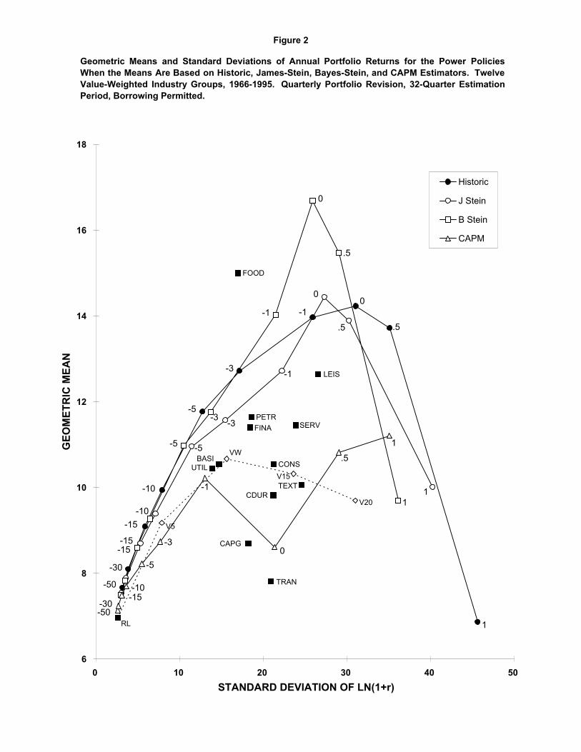
Figure 2

Geometric Means and Standard Deviations of Annual Portfolio Returns for the Equal-WeightedIndustry Groups, the Equal-Weighted Benchmark Portfolios, and the Power Policies With andWithout Target-Weight Constraints, 1966-1995, Borrowing Permitted. Target-Weight ConstraintsAre Industry Market Values Plus or Minus 5%.

RL

V20

V15

VW

V5

.5

0-1

-3

-5

-10

-15

-30

-50

1

-15

-10

-5

-3

-1

0

.5

1

-15

-5

-3

-1

0

.5

1

-50-30

-15-10

-5

-3

-1

0

.51

SERV

LEIS

CONS

TEXTCDUR

CAPG

TRAN

BASIUTIL

PETRFINA

FOOD

6

8

10

12

14

16

18

0 10 20 30 40 50STANDARD DEVIATION OF LN(1+r)

GEO

MET

RIC

MEA

N

Historic

J Stein

B Stein

CAPM

Geometric Means and Standard Deviations of Annual Portfolio Returns for the Power PoliciesWhen the Means Are Based on Historic, James-Stein, Bayes-Stein, and CAPM Estimators. TwelveValue-Weighted Industry Groups, 1966-1995. Quarterly Portfolio Revision, 32-Quarter EstimationPeriod, Borrowing Permitted.

Figure 3

-15 -10 -5-3

-1

0 .5

-3 -1

0

.5

1

-15-10-5 -3

-1

0

1

-50-30-10

-5 -3 -10

.5 1

V5RL

VW

V15

V20

SERVLEIS

BASI UTIL

CAPG

CDUR

FINA

PETR

FOOD

TEXT

CONS

TRAN

-5

-4

-3

-2

-1

0

1

2

3

4

5

6

7

8

9

10

11

- 5 10 15 20 25 30 35 40 45 50 55

STANDARD DEVIATION OF LN(1+r)

GEO

MET

RIC

MEA

N

Historic

J Stein

B Stein

CAPM

1

Geometric Means and Standard Deviations of Annual Portfolio Returns for the Power PoliciesWhen the Means Are Based on Historic, James-Stein, Bayes-Stein, and CAPM Estimators. TwelveValue-Weighted Industry Groups, 1966-1981. Quarterly Portfolio Revision, 32-Quarter EstimationPeriod, Borrowing Permitted.

View publication statsView publication stats