applying monte carlo simulation to model a sales …

APPLYING MONTE CARLO SIMULATION TO MODEL

A SALES PROCESS FOR FORECASTING FUTURE

SALES

A case study for a Finnish recruitment consulting company

Master’s Thesis

Antti Merisalo

Aalto University School of Business

Information and service management

Spring 2018

Aalto University, P.O. BOX 11000, 00076 AALTO

www.aalto.fi

Abstract of master’s thesis

i

Author Antti Merisalo

Title of thesis APPLYING MONTE CARLO SIMULATION TO MODEL A SALES PROCESS FOR

FORECASTING FUTURE SALES

Degree M.Sc. Economics

Degree programme Information and Service Management, ISM

Thesis advisor(s) Markku Kuula

Year of approval 2018 Number of pages 49 Language English

Abstract

For years, sales forecasting has been seen as an important base for a company’s operative

planning process. Effective sales forecast has the power to change the perspective of the

whole company’s business model from reactive to proactive. There exists a wide and

colorful literature regarding various sales and demand forecasting methods, their usage, and

impact for the business from various angles. In addition, its importance for customer

relationship management has been identified. However, in the academic literature there has

scarcely been discussion on how to actually utilize company’s internal CRM systems to aid

in sales forecasting.

In this thesis, I aim to contribute to this topic by modelling a multi-stage sales process

of a Finnish recruitment company by utilizing their internal CRM data. Modelling is done

by using Monte Carlo Simulation of repeated random sampling. The resulting model can be

used to analyze the whole process and its uncertainties as a whole or dig deeper into a

specific sales stage. Furthermore, it can also be used to forecast short-term sales volumes.

The proposed simulation model will be benchmarked to a number of commonly used

quantitative forecasting methods and the results show that the simulation model outperforms

them in terms of forecasting accuracy and forecasting bias. The dual-sided role of the model

is to aid in forecasting and act as a decision-support-system (DSS) when the case company

is assessing their resourcing alternatives and their probable outcomes throughout their value

chain.

Keywords Monte Carlo, Simulation, Sales Forecasting, Stochastic, Model, Quantitative,

Statistics

Aalto-yliopisto, P.O. BOX 11000, 00076 AALTO

www.aalto.fi

Maisterintutkinnon tutkielman tiivistelmä

ii

Tekijä Antti Merisalo

Työn nimi APPLYING MONTE CARLO SIMULATION TO MODEL A SALES PROCESS

FOR FORECASTING FUTURE SALES

Tutkinto Kauppatieteiden maisterin tutkinto, KTM

Koulutusohjelma Tieto- ja palvelutalouden johtaminen

Työn ohjaaja(t) Markku Kuula

Hyväksymisvuosi 2018 Sivumäärä 49 Kieli Englanti

Tiivistelmä

Jo vuosien ajan myynnin ennustaminen on koettu tärkeäksi perustaksi yrityksen

operatiiviselle suunnittelulle. Tehokas myynnin ennustaminen mahdollistaa yrityksen

liiketoimintamallin näkökulman muuttamisen reaktiivisesta proaktiiviseksi. Myynnin ja

kysynnän ennustamisesta on jo olemassa laaja ja värikäs kirjallisuus liittyen näiden

metodeihin, käyttötarkoituksiin sekä liiketoimintavaikutuksiin. Lisäksi myynnin

ennustamisen tärkeys asiakassuhteiden johtamiselle on yleisesti tunnistettu. Kuitenkin,

akateemisessa kirjallisuudessa on ollut niukasti keskustelua siitä, kuinka tosiasiassa

hyödyntää yrityksen sisäisiä asiakassuhteiden johtamisjärjestelmiä (CRM systems)

myynnin ennustamisessa.

Tässä teesissä tuon panokseni tähän keskustelunaiheeseen mallintamalla suomalaisen

rekrytointiyrityksen monivaiheisen myyntiprosessin hyödyntämällä heidän sisäistä CRM –

dataansa. Mallinnus tehdään käyttäen hyväksi Monte Carlo simulaatiota. Tuloksena

saatavaa mallia voidaan käyttää analysoimaan koko myyntiprosessia ja sen epävarmuuksia

kokonaisuutena tai kaivautua syvemmälle yksittäisiin myyntivaiheisiin. Sen lisäksi mallia

voidaan hyödyntää ennustamaa yrityksen lyhyen aikavälin myyntivolyymeita.

Tutkielmassa esiteltyä simulointimallia verrataan muutamaan yleisesti käytettyyn

kvantitatiiviseen ennustemetodiin ja saatujen tulosten perusteella malli suoriutuu paremmin

kuin mitkään verrokeistaan ennustetarkkuuden sekä biasoituneisuuden puolesta. Mallin

kaksi roolia ovat auttaa myynnin ennustamisessa sekä toimia päätöksenavustamis-

järjestelmänä (DSS), kun yritys puntaroi resursointivaihtoehtojaan ja näiden todennäköisiä

vaikutuksia läpi arvoketjunsa.

Avainsanat Monte Carlo, Simulaatio, Myynnin ennustaminen, Stokastinen, Malli,

Kvantitatiivinen, Tilastollinen

iii

Acknowledgements

I would like to take this moment to thank the people and instances that have aided me in my

endeavors with this master’s thesis.

First, I would like to thank my supervisor, Professor Markku Kuula for guiding me

throughout the writing and research process. Your comments helped me move forward and

you were a great aid in planning and scheduling the workload so that I could efficiently carry

out this project.

Second, I would like to thank Assistant Professor Pekka Malo for sparring me with

the methodology choices applied in this thesis. Without our chats regarding the methods,

this thesis would be nothing but skin and bones. Fortunately, now it has also some concrete

meat in it making the research more fruitful.

Third, I would like to thank the case company in question for providing me this

marvelous opportunity to work with you and for providing the data needed to carry out this

research successfully. Without you people, this project would not have been possible. I

would especially want to thank your finance department with your help with the data and by

discussing your goals and needs regarding the project that inspired me to give my best. I

hope that our paths cross in the future as well.

Fourth, I would like to thank Mr. Eskelinen for being my partner in crime throughout

the whole journey in Aalto School of Business. You have been a great source of inspiration

and I have thoroughly enjoyed our enlightening discussions and arguments that have boosted

my creativity.

iv

Table of Contents

Acknowledgements ............................................................................................................. iii

1 Introduction ................................................................................................................. 1

1.1 Motivation for the topic .................................................................................................. 1

1.1.1 Sales versus Demand .................................................................................................... 2

1.1.2 Gains for the industry ................................................................................................... 2

1.2 Research questions .......................................................................................................... 3

1.3 Research methodology .................................................................................................... 4

1.4 Structure of the thesis ..................................................................................................... 5

2 Sales forecasting methods and their usage – a literature review ............................ 7

2.1 Qualitative methods ........................................................................................................ 7

2.2 Quantitative methods ..................................................................................................... 9

2.3 Quantitative methods as Decision Support Systems – an optimal approach .......... 10

3 Theoretical framework –Stochastic processes and Monte Carlo Methods .......... 12

3.1 Stochastic versus deterministic models ....................................................................... 12

3.2 Monte Carlo methods ................................................................................................... 13

4 Analysis & Implementation ...................................................................................... 16

4.1 The case company and sales process ........................................................................... 16

4.2 Sales organization and its roles .................................................................................... 17

4.3 Sales process as a constructed mathematical model .................................................. 18

4.4 Description of the data ................................................................................................. 21

4.5 Parameter estimation ................................................................................................... 23

4.6 Interface to control the simulation .............................................................................. 24

4.6.1 Simulation of a generic month ................................................................................... 24

4.6.2 Visual presentation for predefined scenarios, a three-month forecast ........................ 26

4.7 Fit of the model – Parameter percentage errors ........................................................ 26

4.8 Fit of the model - Histogram comparison of simulated and actual results by role . 28

4.9 Out-of-Sample evaluation: Performance of the model .............................................. 31

4.10 Limitations and assumptions of the model ................................................................. 33

4.10.1 Lead-time from succesful meeting to an opened case ............................................ 33

4.10.2 Deviations from the defined sales process progress ............................................... 34

4.10.3 Assumptions in distributions .................................................................................. 35

4.10.4 Assumption of independence ................................................................................. 36

4.10.5 Market saturation and abundance of leads ............................................................. 36

v

5 Conclusions ................................................................................................................ 37

5.1 Managerial Implications: Two audiences – One purpose ......................................... 37

5.2 Performance of the model ............................................................................................ 38

5.3 Managerial Implications: GIGO ................................................................................. 38

5.4 Further development of the model .............................................................................. 39

5.5 Further research regarding distinction between sales and demand ........................ 40

6 References................................................................................................................... 41

List of Tables

Table 1: Input-output model for the simulation run ............................................................ 21

Table 2: Structure of sales activity data............................................................................... 22

Table 3: Structure of data regarding succesful sales ........................................................... 22

Table 4: Structure of data regarding employments ............................................................. 23

Table 5: Structure of aggregated monthly panel data .......................................................... 23

Table 6: Estimated simulation parameters by role .............................................................. 24

Table 7: Role-specific percentage errors between simulated and actual parameters .......... 27

Table 8: Forecasting accuracy and bias comparison ........................................................... 32

List of Figures

Figure 1: Typical B2B-service sales process ......................................................................... 3

Figure 2: Sales funnel and scope of the simulation ............................................................. 16

Figure 3: Illustration of part of the simulation dashboard. Monthly call amounts .............. 25

Figure 4:Three-month simulated forecast for the sales process .......................................... 26

Figure 5: Account Manager histograms .............................................................................. 28

Figure 6: Account Manager - Novice histograms ............................................................... 29

Figure 7: Coordinator histograms ........................................................................................ 30

Figure 8: Team Leader histograms ...................................................................................... 30

Figure 9: Director histograms .............................................................................................. 31

Figure 10: Test-period Error terms by forecasting model ................................................... 33

Figure 11: "Chaotic" illustration of the sales process .......................................................... 35

vi

List of Equations

Equation 1: Deterministic model example………………………….……………………...12

Equation 2: Stochastic model example………………………….………………………....13

Equation 3: Call distribution……………………………………….……………………....18

Equation 4: Booked meetings’ distribution……………………….……………………......19

Equation 5: Done meetings’ distribution………………………….……………………….19

Equation 6: Alpha parameter estimation.………………………………………………….20

Equation 7: Case distribution……………………………………………………………....20

Equation 8: Case distribution with lead-time effect………………………………………..34

Equation 9: Beta parameter estimation..…………………………………………………...34

Introduction 1

1 Introduction

In this thesis, I aim to contribute to the field of sales forecasting by researching a multi-stage

sales process in the B2B-service sector. A Finnish case company that works in the

recruitment industry provides the data for this research. I start off by inspecting the sales

process, its elements, and different roles inside the company. Next, I build a mathematical

model out of the case company’s sales process with the data provided and by consulting with

the specialists within the company. After this, I apply Monte Carlo simulation to generate a

sufficient sample of simulation runs regarding the sales process. This sample can be then

further analyzed by utilizing statistical methods and thus we end up with company-wide

monthly probability distributions for each stage of the sales process. These probability

distributions can then be used to reflect the process’ potential outcomes and to evaluate

uncertainty within the process.

The simulation works as a decision support system for the board of executives and for

the sales management when evaluating themes such as sales and operations resourcing,

bottlenecks of the process, revenue generation, and critical volumes. The main goal of this

this simulation is to efficiently analyze and visualize the effects of the sales team resourcing

decisions to the actual sales volumes in terms of opened case assignments. This can also be

used to generate sales forecasts in the short-term.

1.1 Motivation for the topic

There is no denying the effect of a proper sales forecasting to the business performance of a

company. For years we have witnessed academic consensus about the importance of this

topic, although there have been discrepancies in the literature about proper forecasting

methods for different situations. Sales forecasting can be seen as a crucial base for planning

a multitude of firm’s other operating activities (Boulden, 1958). If we disregard sales

forecasting, we are only able to respond retroactively to the outcome of the business. This

may lead to stockouts, low quality production, slack resources, insufficient customer service,

and ultimately decreased performance of the company in its competitive environment (Fildes

& Hastings, 1994).

Introduction 2

1.1.1 Sales versus Demand

Plenty of the dialogue in sales forecasting literature has been concentrated to industries

that focus heavily on physical products and to industries that traditionally include heavy and

complex supply chains. However, the literature regarding service industries has not gained

as much attention. Furthermore, an emphasis on sales forecasting literature has been to

forecast demand rather than the actual outcome of sales activities of a company. This earlier

research has many times taken sales resources for granted and focused largely on the outside

market demand, assuming that all demand converts to sales. I deem that it is important to

draw a distinction between these two and try to separate the effect of a company’s internal

sales efforts to those of the external demand that stems from outside the company.

My approach turns this paradigm of outside demand forecasting around into a

company’s internal sales forecasting as in this thesis I take the viewpoint of a small &

medium business where resources are limited and there is evidence regarding substantial

demand in the markets for their offering. The aim of this approach is essentially to help the

company to better estimate the effects of its various sales resourcing choices and sales efforts

to better plan their resourcing throughout their whole value chain.

1.1.2 Gains for the industry

Typically, recruitment industry is heavily human capital intensive and each

recruitment case takes a significant amount of working hours to deliver it successfully. These

companies’ most valuable resource are their personnel. Traditionally personnel also amount

as the sole largest cost object in this industry in terms of salaries and other expenses that the

size of the staff generates. In most situations, a company has to consider labor wages as a

fixed-cost object in the short-/medium-term timeline, given the legislation.1 Thus, every new

employee must be seen as a crucial investment decision.

A traditional characteristic of this industry is also a pricing model that is at least

partially success-fee based. However, there is a substantial variance in the monthly sales

volume of new projects, which causes pressure on the operative side. Too low sales

performance causes slack and idle resources in terms of operative working hours that the

company is not able to utilize sufficiently. On the other hand, too rapid increase in sales

volumes causes critical bottlenecks and may lead to failed projects and/or lack of quality in

1 Assuming the Scandinavian legislation base and a company with decent moral standards.

Introduction 3

delivering a project. Given the success-fee based pricing model in the industry, these

bottlenecks can be very costly in the form of lost revenue. These bottlenecks can even nullify

the success of the sales team if the operative side cannot keep up with them. Therefore, the

more reliable and accurate the sales forecasting is the better the company can proactively

ready itself to utilize all its resources effectively. Academic literature (e.g. Fildes &

Hastings, 1994, and Boulden, 1958) shows that clear links exist between successful sales

forecasting and successful planning of operative staff as well as between successful sales

forecasting and high-quality customer service, which ultimately leads to increased business

performance.

1.2 Research questions

Most B2B-service selling companies’ sales pipeline is a

multi-stage sales process instead of a straightforward offer-

and-buy model that includes only one stage. At first stage

there is prospecting to identify potential leads. On second

stage, a salesperson contacts these leads (potential customers)

to book a sales meeting (third stage). The meeting itself is the

fourth stage where an offer is being made to the customer.

The goal of this meeting is the fifth stage, opening of an

assignment/case/project for the customer. Figure 1 on the

right-hand side illustrates the sales-process that is in focus of

my thesis. Due to the lack of available data in the first stage

(prospecting), I have restricted my research only to the four

later stages of this multi-stage process.

My research questions are as follows:

1) How the proposed Monte Carlo simulation can help in estimating the future sales?

2) How the proposed Monte Carlo simulation model performs in comparison to the

base case forecast?

Figure 1: Typical B2B-service sales

process

Introduction 4

As the empirical part of my thesis is done as a case study, during the research I also build

the necessary interface tools for the case company to predict and monitor their short-term

(three months onwards) monthly sales.

1.3 Research methodology

We can treat the sales process described previously on figure 1 as a stochastic process where

each activity has a potential either (1) to carry on to the next stage of a process or (2) to meet

a dead end. In his book, Stochastic processes: a survey of the mathematical theory, John

Lamperti describes stochastic processes as a collection of random variables (Lamperti, 1977)

which is the opposite of more traditional deterministic processes where randomness is not

present.

Typically, sales forecasters have used these deterministic models that produce single

point estimates as output for estimating future outcomes (Reed & Stephan, 2010). However,

forecasting is never exact but there is always uncertainty and risk associated to it. To deal

with this uncertainty, common methods through history have been what-if and scenario

analyses and their variations (Wagle, 1967). In what-if analysis technique, a user changes

the value of one model parameter at a time and records the changes in the model output. In

scenario analysis technique, a user creates predefined scenarios where he/she changes

multiple parameters at once (e.g. scenarios like optimistic, expected, and pessimistic) and

records the changes in the model output. Both methods are useful to identify the most

important variables to the model. Usually, these methods utilize judgmental probabilities for

differing scenarios (Wagle, 1967) that are given by either the analysts or executives in the

company. Methods of this kind are relatively simple to use and understand, and that is why

they have been so popular in the business world throughout the twentieth century.

However, there are a couple setbacks in these methods. First, they only produce a

single potential output at a time, which can be tedious when executives require a wide

enough understanding of risks to aid in the decision-making. Second, these methods itself

do not provide us with any likelihood regarding a certain scenario or outcome. Third, the

judgmental probabilities utilized are very easily prone to subjective biases2 (Hogarth &

Makridakis, 1981) that arise from the fact that humans are by default poor intuitive

2 These subjective biases and reasons for their existence are discussed in more detail in

Section 2.

Introduction 5

statisticians (Kahneman, 2011). Once these biases stealthily establish themselves they are

hard to spot and change and they can easily lead to substantial systematic errors in

forecasting models.

To tackle the problem of systematic bias my aim is to model this process on a

monthly company wide basis by applying the Monte Carlo simulation method to it. That is,

by utilizing repeated random sampling and observing the behavior of this sampling, I

construct a statistical analysis that we can use to study the possible outcomes in the sales

process and to estimate the probabilities of these outcomes. This way we can forecast the

expected levels of different sales activities and outcomes as well as model the uncertainty of

the process without exposing ourselves too much into judgmental bias.

The output of this method provides the case company with monthly probability

distributions for each stage of the sales process. These distributions give the executives an

instant feedback about the likelihoods of possible outcomes. This way they aid in decision

making when the decision maker can visualize the uncertainties and confidence intervals of

the whole process in one glimpse.

1.4 Structure of the thesis

The following second chapter provides the reader with the literature background regarding

the various sales forecasting techniques. As there exists a vast amount of different sales

forecasting techniques and their variations, I will be concentrating on these techniques on

the upper level without going into too much technical detail on all of them. Instead, my focus

will be on the familiarity, adoption, usage, and reception of different techniques. Many of

these techniques are general in a sense that they are not used solely within the field of sales

forecasting but they are utilized to estimate a multitude of other activities and phenomenona

as well. However, I am mainly taking the viewpoint of sales forecasting and business in this

thesis.

The third chapter digs deeper into the theoretical and technical side on the core

elements within my methodology. I go through the topics such as Deterministic and

Stochastic models and Monte Carlo methods.

The Fourth chapter contains the empirical part of the thesis. This includes going

through the data gathered, and the process to be modeled as well as its mathematical

modelling. In addition, I discuss the process of estimating the required model parameters,

going through the simulation process and illustrating the results. I also discuss about the fit

Introduction 6

of the model and give a glimpse to the excel-based interface that has been built to control

the model. I conclude the empirical part by discussing the limitations and assumptions that

are associated within this model.

The Fifth chapter discusses about the managerial implications that this study gives.

As the tool built during the process comes into direct and regular use within the business,

this chapter discusses the topics such as where to focus in the model, how it can be further

developed if need be, and what is crucial for its results to be reliable.

The sixth chapter wraps up the thesis and provides suggestions for future research

regarding the implementing of Monte Carlo processes in the field of sales forecasting.

Sales forecasting methods and their usage – a

literature review 7

2 Sales forecasting methods and their usage – a literature

review

As long as there has been sales of any kind there has also been anticipations regarding future

sales – sales forecasts. Sales forecasting methods are divided into two groups: qualitative

and quantitative techniques. In this section, I will discuss about the different methods of

sales forecasting and how they have evolved during the past decades. I will start with the

qualitative methods including human judgment and intuitions. Second, I discuss about

quantitative methods that draw from the field of statistics. I finish this chapter by providing

what literature suggests as ‘optimal’ combining of qualitative and quantitative methods.

2.1 Qualitative methods

The oldest forecasting methods are qualitative by nature and usually they include judgmental

output by an individual that is responsible about forecasts. In majority of organizations,

forecasts are either solely based on human judgment or judgmental corrections are applied

to the predictions provided by statistical models (Goodwin, 2002).

Qualitative forecasting methods utilize human judgment and their subjective feelings

regarding the topic in question, in this case, the sales. These techniques usually rely on the

insights of executives, consultants, academia, and/or other employees that are well informed

and have substantial insights and expertise regarding the topic to be forecasted. The target

variable to be forecasted can be either a single point value such as next month’s sales or

longer-term developing trend (Lawrence, et al., 2006). It is also relatively common for

executives to set subjective probabilities either in categorical levels or as percentage

probabilities to different scenarios when evaluating future outcomes. Some commonly used

qualitative methods include executive judgment, sales persons’ insights, Panel of executive

opinion, and the Delphi method (McCarthy, et al., 2006).

The literature regarding qualitative forecasting methods has been colorful during last

decades. Their popularity among companies has been substantial (Dalrymple, 1987) and the

most often this has been justified by their ease of use (Luxhoj, et al., 1996). Other proposed

reasons for adopting qualitative forecasting methods have been their cost-efficiency and lack

of data required to effectively utilize quantitative methods instead (Dalrymple, 1987).

Furthermore, also the lack of competence or familiarity among more sophisticated


literature review 8

quantitative methods is shown to be among the reasons why a company would stay utilizing

only qualitative methods (Lawrence, et al., 2006). However, research has proved qualitative

methods as being prone for substantial systematic errors (Hogarth & Makridakis, 1981). This

is largely due to three features of human behavior. These features cause systematic biases to

judgmental forecasts (Fildes, et al., 2009). The features are as follows:

1) The tendency to search for patterns where there is none (Lawrence, et al., 2006),

2) The illusion of control when the process in question is in fact totally random

(Lawrence, et al., 2006), and

3) The illusion of understanding (Kahneman, 2011)

In their researches regarding subjective probabilities, Kahneman and Tversky showed

how human judgment is widely affected by certain intuitive heuristics of our mind such as

representativeness (Kahneman & Tversky, 1972) and availability (Tversky & Kahneman,

1973). According to the representativeness heuristic, the subjective probability of an event

is based on how similar it is compared to its mother population. The availability heuristic

instead implies that our intuitive judgment regarding probabilities and frequencies is

influenced by the ease with which similar outcomes come to our mind. These findings from

the field of cognitive psychology clearly illustrate how our judgmental forecasting can be

blinded quite easily and how we have to be cautious about ourselves when we are

implementing qualitative methods in our forecasting.

As we can observe, qualitative forecasting has gained some criticism towards it in

the academic literature during the past decades. Despite this, qualitative forecasting

techniques are not all bad and they will not necessarily lead us always to huge forecasting

errors that are drastic and hazardous to the business and decision-making. One must simply

be cautious when utilizing judgmental forecasts and learn to think critically towards her/his

own intuitions. In addition, a great way to enhance qualitative forecasting accuracy is to

collaborate with multiple experts within the area with techniques such as Jury of executive

opinion (Mentzer & Cox, 1984) and Delphi method (Murry Jr. & Hammons, 1995). There

exists numerous studies such as (Rohrbauhg, 1979), (Press, 1978), and (Armstong, 1986)

suggesting that judgmental forecasting accuracy increases when multiple individual

forecasts are aggregated compared to individual executives’ forecasts.


literature review 9

In more recent years however, a role of qualitative judgment has evolved remarkably

in the academic literature. During the eighties, it was relatively common to read warnings

from researchers against judgmental forecasting, e.g. (Hogarth & Makridakis, 1981), but

nowadays there seems to be clearer acceptance about its role in the field of forecasting

(Lawrence, et al., 2006). Paul Goodwin is among the advocates speaking on behalf of

management judgement forecasting methods. According to him, all forecasts involve

judgement (Goodwin, 2002). This will hold even though the forecast would be a product of

extremely sophisticated computational algorithm. Some areas where there always exists

human judgement include e.g. the choice of method, model, predictors, and data set.

2.2 Quantitative methods

The second main category within forecasting techniques are quantitative methods.

Quantitative forecasting methods are mathematical by nature and they rely heavily on

statistical analysis and utilizing historical data. In majority of these methods, the common

denominator is that methods aim to predict future outcomes as a function of historical data

(Armstrong, 2001). The number of quantitative forecasting methods available today is vast

and their complexity ranges from simple averages and naive forecasts all the way to highly

sophisticated machine learning algorithms that make use of tremendous amounts of

computing power and produce complicated black box models that an ordinary human mind

is not able to comprehend. In addition, technological development and ever-increasing

computational power enable us to continually utilize more and more sophisticated sales

forecasting solutions.

Multiple academic researches regarding the usage and performance of various

forecasting methods has been conducted throughout recent decades, e.g. (Dalrymple, 1987)

and (Lawrence, et al., 2006). Disturbing finding is that the usage of quantitative forecasting

techniques has steadily remained as an underdog compared to qualitative methods even

though there is clear evidence that properly utilized quantitative methods outperform

qualitative methods invariably (McCarthy, et al., 2006).

There is a clear negative correlation between the use of a specific quantitative

technique in business environment and its level of complexity (Mentzer & Cox, 1984). The

most widely used methods are relatively simple by nature. These methods include e.g.

moving average, trend line projection, and exponential smoothing. More complex methods,


literature review 10

such as simulation and box – Jenkins methods are much less used (Mentzer & Cox, 1984).

The literature argues that the main reasons for not adopting certain quantitative techniques

are due to the lack of expertise, insufficient data, and prejudices from judgment focused

firms towards quantitative methods (McCarthy, et al., 2006). In other words, companies do

not have means to use them, they do not believe in the models’ efficacy over the executives

own gut feelings, or the management is afraid to adopt tools that they themselves will not

necessary understand.

2.3 Quantitative methods as Decision Support Systems – an

optimal approach

As stated before, organizations use judgmental forecasting widely. The essence here is not

that whether to use or not use ones individual judgment but instead when, where, and to what

extent to use it to get the best out of it. Dating back to 1986 another pioneer in this area,

Michael Lawrence argumented how combining both judgmental and statistical forecasts

together provides enhanced forecasting performance when compared each one individually

(Lawrence, et al., 1986). Qualitative adjustments to quantitative forecasts are justified

especially when regular time series patterns are interfered by extraordinary events that are

foreseeable (Goodwin, 2000). However, Goodwin points out how judgmental forecasters in

fact tend to make redundant alterations to decent quantitative forecasts without decent

evidence to justify their actions. They simply want to do so without asking themselves the

question ‘why am I doing this?’

As we saw in this chapter, qualitative methods and judgment have their own glorious

place in the forecasting process and we should never try to avoid it. We merely have to be

vigilant when and where we tend to resort to these techniques. According to the research,

there are two places in the forecasting chain where we should use qualitative judgmental

analysis:

1) In the beginning of the forecasting process before the quantitative part when

identifying what we are trying to forecast. Here we have to focus on choosing the

right methods, model, data sets, and predictors.


literature review 11

2) In the end of the forecasting process as a cherry on top when the executive/analyst

responsible of forecasting can have the most out of all the knowledge that the

process has gathered from quantitative sources before decision-making. Here we

have to focus on whether we need to adjust the quantitative forecasts and if we

do, to what extent we have adjust them and especially why we have to adjust

them in the given situation.

The second factor above illustrates how the human should always have the last word in the

forecasting process by validating the results and choosing actions based on them. Between

these two points, there exists room for the quantitative analysis and sophisticated forecasting

systems that work as a decision support systems (DSS). That is – their role indeed is to aid

and support in making the business decisions but not to make them on behalf of the human

mind.

Theoretical framework –Stochastic processes and

Monte Carlo Methods 12

3 Theoretical framework –Stochastic processes and

Monte Carlo Methods

The simulation model discussed later in fourth section is effectively a stochastic model. This

section discusses briefly the differences between stochastic and deterministic models and

introduces the concept of Monte Carlo methods which I will be utilizing in the empirical

part of the thesis.

3.1 Stochastic versus deterministic models

There are two types of quantitative forecasting models available: Deterministic and

stochastic. By definition, deterministic models are mathematical models where their output

values are solely predetermined by their input values. These models do not involve any

randomness in their future states and due to this; they will always produce the same results

from the same initial conditions. Deterministic models can be seen as more traditional and

their output is always either a single point estimate, single set of point estimates, or a single

trend (Taylor & Karlin, 1998). A typical example of a deterministic model is e.g. a model

including an amount of debt (P) with a fixed interest rate (r) for a given number of years (Y)

that is compounded monthly (m). The model itself is merely the equation described below

and it illustrates us the total payment (F) that we have to make during the Y years:

𝐹 = 𝑃 ∗ (1 + 𝑟𝑚⁄ )𝑌𝑚 (1)

As you can see, there is no randomness present and with a given set of starting parameters

(P, r, m, and Y) we always get the same result that is ‘predetermined’.

Stochastic models on the other hand always include randomness to some extent, thus

meaning that the same initial input of the model does not always produce the same output.

The word “stochastic” itself is derived from the Greek word “stochastikó” which means

randomness. Because stochastic models are subject to randomness, they produce a set of

probable output values. From these values, we are able to produce different probability

distributions that we can use to evaluate the likelihood of a certain outcome in the model

(Taylor & Karlin, 1998). The most common appearance of stochasticity within the model is



through an individual model parameter that can have a multitude of probable values. A

simple example of a stochastic process is the sum of two six-sided dice:

𝑆 = 𝐷1 + 𝐷2, where 𝐷1 𝑎𝑛𝑑 𝐷2 ~𝑈{1,6}3 (2)

The previous equation is indeed simple, but unlike the first deterministic equation, this

equation does not always produce the same output as the possible inputs can vary randomly.

Due to this, it is often redundant to calculate the stochastic model only once. Instead, by

repeating the calculation a sufficient amount of times by using a random number generator

we can derive likelihoods for the possible outcomes of a model.4

Even though we have two opposite classes of models, the phenomena of the real

world are usually not purely deterministic or stochastic but they have properties of both. The

choice to model a phenomenon as one or the other is purely the choice of the observer

(Taylor & Karlin, 1998). Generally, deterministic models are simpler than stochastic models

that tend to be more detailed. However, one should not be fooled that the more complex

model would always be better. For a given phenomenon, there is no that kind of thing as the

best model (Taylor & Karlin, 1998). Instead, the purpose for which the model has been

created is the factor against which the model should be evaluated and the pragmatic ultimate

criterion in this evaluation is the usefulness of the model. It is not unheard-of that for a

certain phenomenon, two or more differing models are created if they serve separate

purposes.

3.2 Monte Carlo methods

Originally named by the administrative area of Monaco, famous for its gambling casino,

Monte Carlo simulation methods (or Monte Carlo methods) refer to the computerized

methods where repeated random sampling is utilized to estimate the probability distribution

3 For those not familiar with the mathematical notation this implies that 𝐷1 𝑎𝑛𝑑 𝐷2 have a

discreet uniform distribution between values on and six. I.e. they can have any whole number

value between one and six with an equal probability. 4 In the model in question, the number of outcomes is relatively small and probabilities can

also be calculated by hand. However, in many business cases, the number of outcomes is

vast or even infinite and in these cases, it is not feasible to determine separately all possible

scenarios.



of a process’ potential outcomes (Kroese, et al., 2014). The main idea in Monte Carlo

techniques is to repeat the process numerous times to obtain sufficiently large sample base

of outcomes. These outcomes we can then analyze by using the methodologies of statistical

inference to the sample created.

Monte Carlo methods are relatively popular today and they have been used in a

variety of fields including e.g. Physics (Tuchin, 2007) , Industrial Engineering (Elperin, et

al., 1991), and Finance (Boyle, 1977). Kroese, et al. (2014) propose the following four

reasons for their popularity:

Efficiency and ease of use: The algorithms inside Monte Carlo methods are

usually relatively simple and scalable. Complex models of real world can be

narrowed down to a combination of rules easily implemented on a computer,

which helps us to observe more general models than traditional analytic

techniques would allow us to observe.

Randomness as a strength: In addition to mirror the randomness of real-life

systems, the intrinsic randomness within Monte Carlo methods allows us to

explore also deterministic problems and their search space through stochastic

algorithms.

Insight into randomness: Not only Monte Carlo methods utilize randomness in

them, but their output also works as a means for us to better understand the

behavior of random systems and the data they possess.

Theoretical justification: The mathematical and statistical literature on Monte

Carlo methods is already immense and ever growing. This research enables us to

create more precise and efficient algorithms.

In addition, Monte Carlo simulation techniques have very practical advantage to the

traditional what-if and scenario analyses in terms of analyzing uncertainty and/or risk. As

we discussed earlier, Monte Carlo methods tend to give a range of potential outcome values

and their probabilities as an output. Deterministic models instead tend to give only single

point estimates as an output. Historically, the most common methods for analyzing



uncertainty in models have been sensitivity and scenario analyses (Wagle, 1967). As

discussed earlier, these methods work so that by changing the value of one or more key

variable(s) in the model, a change in the output is observed and with this, the observer can

identify the most important variables in the model. However, these tools present the outcome

of the model as a sure thing without considering any possible fluctuation in its value.

Furthermore, all the probabilities within these models tend to be only subjective point

estimates placed by the executives and in chapter 2.1, we discovered how prone these

judgmental estimates are for bias. Monte Carlo simulation beats these limitations as it itself

produces the probability distribution of possible outcomes as its output (Reed & Stephan,

2010). Due to this, the Monte Carlo simulation is also a useful tool for visualizing the

uncertainty in the model for the decision maker.

Analysis & Implementation 16

4 Analysis & Implementation

In this section, I go through the empirical part of my thesis. The main idea is that after reading

the section the reader has a decent understanding regarding how the simulation process was

conducted and what are the main functionalities of the final forecasting tool. I start by

presenting the case company, sales process, and its mathematical model. I continue by

describing the utilized data and by describing the different sales team roles that I am

including in the simulation. Next, I present the functionalities of the interface and estimate

the initial parameters. After this, I compare the fit of the model to that of actual results and

compare the model performance to numerous benchmark models. I conclude the section by

discussing the limitations and assumptions that this model holds.

4.1 The case company and sales process

The case company in question is a rapidly growing Finnish recruitment-consulting firm with

a variety of differing service lines. These service lines range from basic recruitment services

such as direct recruitment or employee leasing all the way to feasibility assessments and

tailored large scale consulting, trainee, and branding solutions.

In this thesis, the focus of the research will be on the simulation of basic recruitment

services such as direct recruitment to a customer’s payroll or leasing an employee to a

customer on behalf of the case company. This is due to the simpler sales process of these

services compared to larger solution offerings whose sales process cycle can be multiple

times longer, may involve a number of personnel from both the customer and supplier side,

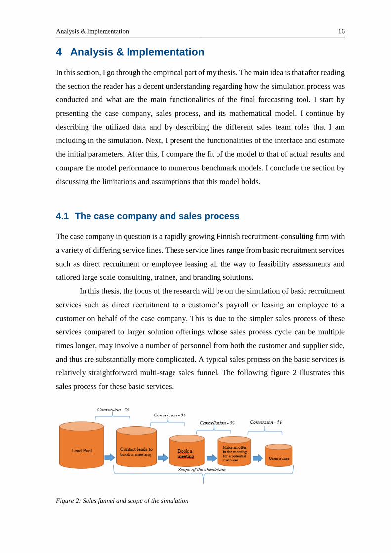
and thus are substantially more complicated. A typical sales process on the basic services is

relatively straightforward multi-stage sales funnel. The following figure 2 illustrates this

sales process for these basic services.

Figure 2: Sales funnel and scope of the simulation


I have to emphasize that as all models, this too is only a simplified version of the real world.

A number of assumptions are made due to data restrictions. First, the sales funnel here is

illustrated as a straight-line one-way process where the two possible outcomes are either up

or out. In reality however, there is a possibility that a salesperson has to take multiple

repetitions in any of the stages for the same potential customer before he/she may proceed

forward in the funnel. This may be due to changes in proposed contractual terms, customer

hesitations, or because the decision-making in customer-side includes multiple persons.

Second, the funnel is outbound focused and assumes that it is always the salesperson who

contacts the customer. However, there is always a possibility for inbounds where the

customer contacts the company. Third, on rare occasions, steps can be skipped and the initial

contact may already turn out for a succesful sale.

4.2 Sales organization and its roles

The sales organization consists of various roles whose focus and goals vary from each other.

Together with the case company, I have identified five different key roles within the sales

team that I am implementing to the simulation. These roles have either differing emphasis

on their duties within the team or differing work experience. The Monte Carlo simulation

that I generate in this study includes these roles with their individual estimated parameters

throughout the sales process. The roles are Director, Team Leader, Coordinator, Account

Manager, and Novice Account Manager.

Director: In charge of the sales team and its development as a whole. Productive in

its sales cases due to his/her expertise and experience. However, highly limited

amount of working hours goes to routine sales work. This has an adverse effect on

sales activity volumes.

Team Leader: In charge of the performance of its own sales team. Also productive

in his/her salesmanship but due to obligations towards the team, possesses a limited

amount of time towards routine sales work. Also in this role, the time constraint has

an effect on sales activity volumes.


Coordinator: Assisting role within the organization. Aids account managers and

contacts potential leads with sales calls. Aims to book sales meetings for account

managers. This role only books sales meetings but does not usually attend them

his/herself.

Account Manager: The main salesperson role that uses a majority of his/her working

hours to the sales process. Engages in every part of the sales process.

Account Manager – Novice: Similar role to that of an account manager. However,

possesses less experience. In the simulation, account managers with less than 4

months of working experience are given a novice status.

When it comes to carrying out the sales process these roles can be classified into two groups.

Account Manager, Novice Account Manager, and Coordinator create the core group that

creates the most of the sales volume in all activities. They also amount for the substantial

majority within the team with their share laying around 85% - 95% percent of the total sales

team headcount. Team Leader and Director roles instead generate the supportive group due

to their somewhat different tasks, limited working hours within the ordinary sales process,

and significantly smaller headcount compared to the first group.

4.3 Sales process as a constructed mathematical model

This chapter illustrates the mathematical representation of a sales process illustrated in the

Figure 2 in the chapter 4.1. First, I go through each step of the process individually. After

that, I will summarize the required parameters and present the input-output model for the

individual simulation run. All relevant limitations and assumptions regarding the model have

been compiled to the section 4.10. “Limitations and assumptions of the model”.

The amount of monthly calls that a certain individual in sales team makes is assumed

to follow normal distribution with mean 𝜇 and standard deviation 𝜎. Thus, we can denote

the amount of calls during month t as:

𝐶𝑎𝑙𝑙𝑠𝑡 ~ 𝑁(𝜇𝐶𝑎𝑙𝑙𝑠, 𝜎𝐶𝑎𝑙𝑙𝑠) where 𝐶𝑎𝑙𝑙𝑠𝑡 ∈ (0, ∞) (3)


It is noteworthy that the normal distribution is truncated to only include non-negative values,

as there cannot exist a negative amount of sales calls with anybody on the sales team.

The outcome of a succesful call from a sales person is a booked sales meeting with a potential

customer. Not all calls are succesful but there is a certain conversion rate from calls to

booked meetings that varies in time. Simply put it, there are only these two5 possible

outcomes from a sales call: Failure or book a meeting. Due to this, the sales call can be seen

as a Bernoulli trial (i.e. binomial trial). Because of the Bernoulli nature of this process we

can estimate the amount of booked meetings during month t by employing binomial

distribution to them. We can thus denote them as following the subsequent distribution:

𝑀𝑒𝑒𝑡𝑖𝑛𝑔𝑠𝐵𝑜𝑜𝑘𝑒𝑑𝑡 ~ 𝐵𝑖𝑛(𝐶𝑎𝑙𝑙𝑠𝑡, 𝐶𝑜𝑛𝑣𝑒𝑟𝑠𝑖𝑜𝑛%𝐶𝑎𝑙𝑙𝑠) (4)

There are a couple of attributes in booked meetings. First, not all meetings ever happen.

Instead, some of them might be postponed or cancelled either by the customer or by the sales

person. Thus, there is a certain rate of cancellation, c. Second, there is a lead-time between

when a meeting has been booked with a customer on the phone and when it really is due.

Because of this lead-time, some meetings fall due later than the ongoing month. This means

that sales meetings that are done in the month t are a sum of all booked sales meetings from

previous months that fall due on month t subtracted by the ones that have been canceled. As

a mathematical equation, we can denote this relationship as:

𝑀𝑒𝑒𝑡𝑖𝑛𝑔𝑠𝐷𝑜𝑛𝑒𝑡= (1 − 𝑐𝑡) ∑ (𝛼𝑡−𝑚 ∗ 𝑀𝑒𝑒𝑡𝑖𝑛𝑔𝑠𝐵𝑜𝑜𝑘𝑒𝑑𝑡−𝑚

)

𝑛

𝑚=0

(5)

, where 𝛼𝑡−𝑚 is the proportion of booked meetings during month t-m whose due date falls

to the month t. 𝑐𝑡, on the other hand is the cancelation rate of booked meetings in month t.

The values of parameters are estimated through the lead-time of meetings,

(𝐿𝑡𝑀𝑒𝑒𝑡𝑖𝑛𝑔), which is calculated as the difference in days between the due date of a meeting

and the date when a sales person booked the meeting and added it to the CRM. We can thus

denote that:

5 In reality, in rare cases a sales call can also produce another sales call later on or jump

straight into a stage of succesful sale.


𝛼𝑡 =𝐿�̅�𝑀𝑒𝑒𝑡𝑖𝑛𝑔

𝑡

𝑑𝑡

(6)

, where 𝐿𝑡𝑀𝑒𝑒𝑡𝑖𝑛𝑔 ~ 𝐸𝑥𝑝(λ) and 𝑑𝑡is the amount of days in the month t. However, sample

data that I have available in this thesis shows that significant majority of meetings falls due

within the ongoing month and the following month. Thus, my simulation model is restricted

to these months by using the average of lead-time instead of utilizing an exponential

distribution of lead-time, which would also lead to exponential distribution of different

parameters.

Moving forward to recruitment assignments (later referred to as ‘cases’) opened

during month t, these are the outcome of a succesful sales meeting. As well as with the calls

not all sales meetings are succesful. Instead, we can derive a conversion rate to done sales

meetings that defines how many cases are opened from done sales meetings during month t.

Similar to calls; we can treat this sales stage also as Bernoulli trial and estimate the amount

of opened cases during month t by employing binomial distribution to them. We can then

denote them as following the subsequent distribution:

𝐶𝑎𝑠𝑒𝑠𝑡 ~ 𝐵𝑖𝑛(𝑀𝑒𝑒𝑡𝑖𝑛𝑔𝑠𝐷𝑜𝑛𝑒𝑡 , 𝐶𝑜𝑛𝑣𝑒𝑟𝑠𝑖𝑜𝑛%𝑀𝑒𝑒𝑡𝑖𝑛𝑔𝑠) (7)

Given these equations, we can simulate the monthly behavior of sales funnel as long as we

are able to estimate reliably the following parameters:

The average number of calls: 𝜇𝐶𝑎𝑙𝑙𝑠

Standard deviation of calls: 𝜎𝐶𝑎𝑙𝑙𝑠

Average conversion rate from calls to booked meetings: �̅�𝐶𝑎𝑙𝑙𝑠

Average conversion rate from done meetings to opened cases: �̅�𝑀𝑒𝑒𝑡𝑖𝑛𝑔𝑠

The average lead time from booked meeting to done meeting: 𝐿�̅�𝑀𝑒𝑒𝑡𝑖𝑛𝑔

The average lead time from done meeting to opened case6: 𝐿�̅�𝐶𝑎𝑠𝑒

The average cancelation rate of booked meetings7: 𝑐�̅�𝑒𝑒𝑡𝑖𝑛𝑔𝑠

6 &7 Due to the lack of data collected on this item by the case company, there is no reliable

way to estimate these parameters. Thus, I have assumed them as zero in the simulation.

However, the tools provided to the case company include a possibility to speculate with

these parameter values so that they are able to observe and record their effects to the sales.


The four main parameters: 𝜇𝐶𝑎𝑙𝑙𝑠 , 𝜎𝐶𝑎𝑙𝑙𝑠 , �̅�𝐶𝑎𝑙𝑙𝑠 , and �̅�𝑀𝑒𝑒𝑡𝑖𝑛𝑔𝑠 are estimated on a role-

specific level. The latter three parameters will be estimated on a company-wide level, as the

data collection within these data does not yet fully enable us to reliably estimate these

parameters on a role-specific level.

From the table 1 below you can find the input-output model for one simulation run.

This model will be run for each employee of the sales team individually and after that, the

results are aggregated to form company-wide monthly distributions. Total sample size for

the simulation is 5000 runs.

Table 1: Input-output model for the simulation run

Stage Input Distribution Output

I: Calls Mean and standard deviation of monthly

calls by role Normal

Monthly call amounts for each

worker within the sales organization

II:

Booked

Meetings

Call amounts from stage I, average

conversion % of calls by role Binary

Monthly booked meetings for each


III:

Visited

Meetings

Booked Meetings from stage II and from

preceding months for each worker,

average cancellation rate of meetings

and average lead-time of meetings

None

Proportion of meetings that are

visited on a given month for each


IV:

Opened

Cases

Visited sales meetings from stage III,

average conversion % of meetings by

role

Binary

Proportion of opened sales cases for

each worker within the sales

organization

4.4 Description of the data

In my research, I will be utilizing data from the following three data sources:

1) The main data that is the sales activities are derived from the company CRM. This

database includes the individual indexed sales activities and the relevant information

about them. Table 2 below illustrates the structure of this data.


Table 2: Structure of sales activity data

CRM data source

Data item Data type Description

Activity ID String Unique key of different sales activities

Salesperson ID String Identifier of the salesperson

Activity type Binary The type of sales activity: Call or Meeting

Activity added Timestamp Date and time when activity has been added to CRM

Activity done Timestamp Date and time when activity has been done

2) To complement the sales activity information, I will be utilizing data from the case

company’s ERP system where information about ongoing assignments is stored.

From here, I will be extracting information regarding initiated recruitment

assignments. As initiated recruitment assignments will be considered as succesful

sales, I will be matching the customer ID and opening date information from the ERP

to sales meeting information in the CRM to identify what sales meetings exactly

produced succesful sales. Table 3 below illustrates the structure of this data.

Table 3: Structure of data regarding succesful sales

ERP data source


Case ID String Unique key of different customer cases


Case opened Date Date when case has been opened and added to ERP, i.e. when

sales has been succesful

3) As my third data source I will be utilizing the information regarding salespersons’

work role when estimating the required parameters of the simulation process. As I

am constructing a series of monthly simulations, I am utilizing this data to identify

employees’ roles during each month of the sample CRM data. Later on I am referring

to these joined data items as ‘employee months’ – ‘Henkilökuukaudet’. Table 4

below illustrates the structure of this data.


Table 4: Structure of data regarding employments

Personnel data source



Salesperson Role String Identifier of the role within the employment

Employment start date Date Date when the employment has started

Employment end date Date Date when the employment has ended

By aggregating the daily data from these three sources to a monthly format and joining them

together, I am now able to create the following panel data that I can use to estimate the

required monthly parameters per role. The structure of this panel data can be found on the

table 5 below.

Table 5: Structure of aggregated monthly panel data

Aggregated monthly data table


Employee month String Joined data item of salesperson and month

Employee role Category Identifier of employee's role during the specific month

Calls Integer Amount of made sales calls by employee during the specific

month

Booked meetings Integer Amount of booked sales meetings by employee during the

specific month

Done meetings Integer Amount of done sales meetings by employee during the

specific month

Opened cases Integer Amount of opened cases by employee during the specific

month

Call conversion-% Float Proportion of booked meetings to that of sales calls by

employee during the specific month

Meeting conversion-% Float Proportion of opened cases to that of done sales meetings by

employee during the specific month

4.5 Parameter estimation

The parameters are estimated from a time-series sales activity data of six months from

January 2017 to June 2017. To do this, I have first aggregated the daily sales activities and

succesful sales to a monthly data by employees. After this, I have identified the employee

roles monthly, given the data regarding the employee’s work experience and contracts. By

combining these data sets, I have been able to identify all the employee months by role and


thus I can utilize this data set to estimate the parameters. The results of the initially estimated

parameters can be found from the table 6 below. It is noteworthy to mention, that as any

company’s processes, working culture, and efficiency changes constantly through time it is

important to update the parameters on a steady basis so that the simulation can best reflect

the current conditions of the company.

Table 6: Estimated simulation parameters by role

Role

Calls Conversion-%

from calls to

meetings

Conversion-%

from meetings to

sales

Mean St.Dev Mean8 Mean9

Account Manager 91,51 41,63 14,47 % 24,24 %

Account Manager - Novice 72,33 26,82 15,54 % 15,81 %

Coordinator 125,44 38,43 8,36 % ***10

Team Leader 7,43 10,20 40,91 % 67,56 %

Director 12,50 7,01 30,11 % 60,46 %

4.6 Interface to control the simulation

The interface to control the simulation process has been built according to the desires of the

case company. It is an Excel-based tool where emphasis is on the efficiency, ease of use,

and informative visualization of the results. There are two following main visualizations

available regarding the output results, each for a given purpose. Both of these outputs can

be controlled with the same input parameters.

4.6.1 Simulation of a generic month

The first visualization gives us the graphical illustration of all probability distributions

regarding the different stages of the sales process. They include both the histogram formatted

information about the distribution (PDF) as well as the cumulative probability distribution

function (CDF). In addition, each sales stage collects a summary of its core statistical key

8 &9 In the study, averages for conversion rates are estimated from the historical data as

geometric means.

10 By default, Sales Coordinators do not go to meetings but instead only feed their meetings

to Account Managers. Due to this, there is no need to estimate this parameter for this role.


figures in a numerical presentation. These figures are categorized into the following five

classes: Central Tendancy, Spread, Shape, Intervals, and Probabilities. All the other

categories in the summary are calculated in predefined terms but there are two exceptions.

First, in the interval category, in addition to pre-calculated 90% and 95% confidence

intervals, a user has a possibility to inspect a third interval of his/her choice by defining the

confidence parameter alpha. Second, in the probabilities category, a user can check for

individual cumulative probabilities to check for the probability of a specific slice within the

probability distribution. A figure 3 below describes the format of the dashboard11. Similar

visualization is accessible to the executives in all four stages of the simulated sales process.

Figure 3: Illustration of part of the simulation dashboard. Monthly call amounts

This visualization gives the user a comprehensive amount of statistical information

regarding the whole process. It can be used both in the executive level for a comprehensive

visualization for the process and in the analyst level for a more detailed investigation

regarding the sales process and its uncertainties.

11 Due to confidentiality, I have omitted the absolute numerical levels in this figure as well

as bin sizes in the histogram.


4.6.2 Visual presentation for predefined scenarios, a three-month forecast

The second visualization is more simplified and it contains less information in order to

efficiently serve the executive with the estimated future development scenarios regarding

company-wide sales. Furthermore, it provides the executive with the visual information

regarding the uncertainties of each stage of the process. The visualization includes five

predefined scenario levels that are defined from the confidence intervals of the process:

Expected (Mean), Good (Upper 60% confidence interval), Below Average (Lower 60%

confidence interval), Exceptional (Upper 95% confidence interval), and Bad (Lower 95%

confidence interval. Figure 4 below illustrates the format of this visualization12.

Figure 4:Three-month simulated forecast for the sales process

4.7 Fit of the model – Parameter percentage errors

The earlier chapters provided us with the functionalities of the simulation. This chapter

discusses about the output of the model and its fit to the actual data in terms of error rates.

As we have discussed, the probability distributions of each sales process stage work as the

final output of this simulation and for the management they are presented in a company-

wide level. The simulations itself are run in a role-specific level and the final output is simply

12 Also in this visualization, I have omitted the axis values and absolute data table numbers

for confidentiality issues.


an aggregation from all these roles given their amounts in a month to be simulated.13 Due to

the scarcity of company-wide monthly data points in our original sample from H1 – 2017 it

is more practical to evaluate the fit of the model on a role-specific level at this point. Later

on, when more data points are collected both on a role-specific level and on a company-wide

level, it will be feasible to evaluate the fit also on a company-wide level.

The table 7 below describes the percentage differences between the simulated

parameters and actual parameters. We can observe that in terms of the averages in most roles

the differences are relatively small, which would imply a good overall fit.

Table 7: Role-specific percentage errors between simulated and actual parameters

Role Calls Booked Meetings Opened cases

Mean St. Dev Mean St. Dev Mean St. Dev

Account Manager -0,77% -3,19 % 0,44 % 2,48 % 7,81 % -24,15 %

Account Manager - Novice 1,15 % -0,74 % 1,35 % 29,41 % -23,06 % -9,87 %

Coordinator 0,05 % 0,92 % -6,69 % -17,88 % *** ***

Team Leader 2,06 % -5,79 % 68,59 % 177,66 % -4,67 % -29,74 %

Director 40,14 % -27,40 % -11,44 % 14,35 % -58,63 % -38,80 %

The first three roles that form the core group of sales activities perform especially well in

the simulation with their absolute percentage errors remaining well below the ten percent

threshold. The only substantial deviance here is the error in novice account managers’

opened cases. This implies to us that the simulation model somewhat underpredicts their

efficiency in creating succesful sales.

Errors rise somewhat within the supportive group that includes Team Leader and

Director roles. Especially Team Leaders’ booking efficiency and Director’s Call amounts

are overpredicted in the simulation. In addition, Director’s amount of opened cases is

underpredicted in the simulation model. This is highly due to the fact that as there are only

a handful of people possessing these roles the volume of underlying data is not sufficient for

steady parameter estimation regarding these roles. The cause for these deviations can also

be the sloppy usage of CRM system by these leading roles. However, further research would

be required to efficiently find reasons for these role-specific errors.

13 e.g. a typical month could include 15 Account Managers, 3 Novice Account Managers, 7

Coordinators, 2 Team Leaders, and 1 Director.


4.8 Fit of the model - Histogram comparison of simulated and

actual results by role

This chapter contains role-specific histograms of the simulated output as well as actual

outcomes given the employee months. We can use this information to evaluate the fits of the

distributions that the simulation produces to those of their actual counterparts from the real

world. Together with the role-specific percentage errors described earlier, this information

can be used to better enhance the model in the future. Due to confidentiality, I have omitted

the absolute numeric intervals of the bins in the histograms. However, within each activity,

bins have been scaled as equals so that visual comparison would be possible14 between the

simulated data and the actuals but also across different roles as well. Three main stages for

the sales process have been included here and they obey the legend below:

1) Amount of calls made by the role within a month (blue)

2) Amount of meetings booked by the given role within a month (green)

3) Amount of cases opened by the given role within a month (gold)

Figure 5 illustrates the distributions for the role of an Account Manager. In all three main

activities, we can visually observe that the weight of each distribution is approximately

within the same position in both the simulated data and the actual data. Furthermore, there

exists no huge discrepancies between these two. The only notable difference in the center of

gravity can be spotted in opened cases where the center in the actual data is heavily within

the first bin compared to that of the second bin in the simulated data. Simulated data also

tends to be leaning slightly more towards its right-side tail than its actual counterpart and

thus it gives slightly more emphasis to the rare events on the right-hand side.

Figure 5: Account Manager histograms

14 e.g. Bin 1 of calls (blue) has the same numerical range between all roles, etc.


Figure 6 illustrates the distributions created from the Novice Account Managers’ data. As

we can observe, all distributions are more heavily concentrated on the initial bins compared

to the distributions of more experienced Account Managers. This is reasonable as some of

the Novice Account Managers’ time is bound into various orientation processes and they

don’t yet possess their own portfolio of customer Accounts and contacts. Visually, we can

observe that the simulated data is very much in line with its actual counterpart. The slight

exception to this lies in the longer right-hand side tail in the booked meetings.

Figure 6: Account Manager - Novice histograms

Figure 7 shows the actual and simulated distributions for the role of a Coordinator. As

described earlier in the section 4.3, this role focuses on the first stages of the sales process

and feeds their booked meetings to Account Managers instead of attending them personally.

Thus, I have omitted the analysis for the opened cases, as it would be redundant. Coordinator

is the role with the largest sales call volumes. We can also observe this from the data as the

emphasis on this role’s call histograms lies the farthest to the right of all roles. Call

distribution on simulated data describes well the behavior of actual monthly call data.

However, some discrepancy can be seen in the distribution of booked meetings, as actuals

within this activity type seem to behave more erratically than its simulated counterpart.


Figure 7: Coordinator histograms

Figure 8 illustrates the distributions for the role of Team Leader. We have now moved from

the core roles to those of more supporting nature in terms of activity levels. This can also be

seen from the following figure as all distributions are heavily focused around the smallest of

the bins. The behavior of distributions between the previous three roles and the last two is

substantially different as Team Leaders and Directors use much less time to the basic sales

process. Concerning the fit of the simulation within Team Leaders, it is pretty much

consistent with the actual data with the exception of larger right-hand tail given simulated

booked meetings.

Figure 8: Team Leader histograms

The final figure 9 illustrates the distributions for the role of Director. These distributions’

behaviors are very much consistent with the distributions of Team Leader, implying the

similar nature of these roles when it comes to the basic sales process.


Figure 9: Director histograms

Given the results from both the percentage errors and the distribution histograms, we can

say that on a role specific level the simulation model describes the actual behavior of the

sales process relatively well. A somewhat common difference between the simulated data

and the actual was however, that on booked meetings the simulated data has longer right-

hand side tails. In practice, this means that the simulation gives a bit more weight to the

especially positive results that could be categorized as ‘rare events’. In the actual data, these

phenomena are not present. This is mainly due to the larger volume of the simulated data

compared to that of actual monthly data points that we have currently. As time passes and

we collect more data points we can better compare the fit, however the initial results show

that we are on the right path indeed.

Furthermore, significant differences between the roles can be identified which

justifies the parameter estimation in the model by these five roles. With this evidence we can

say that for the core group the model is performing relatively well but for the supporting

group some tweaking of the model could be justified in the future as more data is collected

to enhance our knowledge within these roles.

4.9 Out-of-Sample evaluation: Performance of the model

Previously we focused on the in-sample evaluation of model parameters at a role-specific

level. In this chapter, we will see how the simulation model performs as a whole with out-

of-sample data. The end goal of the model is to help predict the volume and uncertainty of

opened recruitment assignments and thus we focus on this last stage of the sales process in

a company-wide monthly basis.


As the case company has not had any established sales forecasting methods previously

other than the intuitive prediction of sales managers, I will be constructing base case

forecasts based on common quantitative forecasting techniques that are easily adapted to this

type of data and that are widely used among numerous industries. These techniques are

regression analysis and moving average. The testing period for all models is from August

2017 to February 2018 and I use the three commonly used measures for assessing forecasting

accuracy that are Mean Squared Error (MSE), Mean Absolute Deviation (MAD), and Mean

Absolute Percentage Error (MAPE). In addition, I use Mean Error (ME) to assess the bias

of each model.

Three base case forecasts are constructed for the evaluation that are three-month

moving average, OLS regression with the amount of each role separately as explanatory

variables, and OLS regression with the total headcount of all roles as explanatory variable.

The table 8 below presents the measurements for forecasting accuracy.

Table 8: Forecasting accuracy and bias comparison

Expected value of

the simulation

model

3-Month

rolling average

Regression I,

Headcount by

roles

Regression II,

Aggregated

Headcount

MSE 50,32 210,10 511,67 76,63

MAD 5,43 9,33 19,48 6,11

MAPE 9,89 % 16,14 % 39,13 % 10,57 %

ME

(Bias) 0,29 -7,90 -10,14 -3,77

As we can observe, the simulation model outperforms all three models in its accuracy and

most of them with a substantial difference. The only model that comes close in some

accuracy measurements is the second regression model with aggregated monthly headcount

over the total sales team. This model performs also at the same level if we use MAD or

MAPE as the performance measurement. However, it also underperforms if MSE is used as

a performance measure.

Regarding the bias of each model, if ME is used as a bias measurement the simulation

model significantly outperforms all of its benchmarks with possessing only a slight over-

forecast on average. The other three on the other hand possess a substantial over-forecast. A

more detailed illustration of error terms for each model through the seven month testing

period can be found from the figure 10 below. The green plot illustrates for the error terms


of the simulation model. As we can observe, it has the most coherent form without too much

of positive or negative bias.

4.10 Limitations and assumptions of the model

Regardless of the model, it is always only a simplified version of the real world where there

are limitations to it and assumptions have to be made. If this would not be true, we would

not call it a model but reality instead. This chapter clarifies the limitations and assumptions

that I have had to make in the creation of this simulation model.

4.10.1 Lead-time from succesful meeting to an opened case

In reality, there exists a Lead-time from a succesful meeting to opened case. This may be

due e.g. to contract signing issues and information delays between sales personnel and the

operative recruitment team. This phase is analogous to that from booked meeting to done

meeting and means that opened cases during month t are actually sum of succesful sales

meetings from the current and previous months where the opening of the case has been

delayed to the current month. Mathematically this means that following applies:

Figure 10: Test-period Error terms by forecasting model


𝐶𝑎𝑠𝑒𝑠𝑂𝑝𝑒𝑛𝑒𝑑𝑡= (1 − 𝐶𝑡) ∑ (𝛽𝑡−𝑚 ∗ 𝐶𝑎𝑠𝑒𝑠𝑡−𝑚)

𝑛

𝑚=0

(8)

, where 𝐶𝑎𝑠𝑒𝑠𝑡 ~ 𝐵𝑖𝑛(𝑀𝑒𝑒𝑡𝑖𝑛𝑔𝑠𝐷𝑜𝑛𝑒𝑡 , 𝐶𝑜𝑛𝑣𝑒𝑟𝑠𝑖𝑜𝑛%𝑀𝑒𝑒𝑡𝑖𝑛𝑔𝑠) and 𝐶𝑡 is the cancellation

rate of cases that are already agreed upon. Parameter 𝛽𝑡 here is analogous to that of 𝛼𝑡 in

the meetings section and we can estimate it as:

𝛽𝑡 =𝐿�̅�𝐶𝑎𝑠𝑒

𝑡

𝑑𝑡

(9)

, where 𝐿𝑡𝐶𝑎𝑠𝑒 ~ 𝐸𝑥𝑝(λ) and 𝑑𝑡is the amount of days in the month t.

4.10.2 Deviations from the defined sales process progress

The model assumes the sales process as a linear binary process as described in chapter 4.1,

figure 2. Real world however, is more chaotic and the process can jump from one stage to

another more erratically. For example, a sales call can normally lead to a booked meeting or

a dead end but it can also be followed by another call with the same or new contact person

or a case can be opened straight from the sales call, though this would be a rare event. Similar

nonlinear events can be experienced in other stages of the process as well. Furthermore,

instead of outbound lead a sales process can start also with an inbound contact from a

customer as well. Given all the possibilities and excluding the possibility that a current sales

process can also give birth to a new customer lead a more detailed description of the sales

process can be found from the figure 11 below. As we can observe, the system is much more

chaotic and there is a multitude of nonlinear options in the process as well.


Figure 11: "Chaotic" illustration of the sales process

Solid lines describe the linear core process that is the basis of this thesis. Dashed lines include

the other possible interactions between the various state spaces that we encounter in the real

world. Simulation of this type of system would not be feasible through ordinary Monte Carlo

techniques. We could treat this sales system as a Markov Chain process and by utilizing

Markov Chain Monte Carlo methods we could model the chaotic nature of this system.

However, this would need much more available data than the simulation of a linear model

and thus it was not feasible in this thesis.

4.10.3 Assumptions in distributions

In chapter 4.2, I described the distributions for the three key items of the simulation: Call

amounts, booked meetings, and opened cases. I have to emphasize that as in all simulation

models the choices for the distributions of stochastic variables are either estimations or


assumptions. Given the scarcity of data volumes I ended up using the most common and

reasonable distribution assumptions for this case that are normal and binomial distributions.

Normal distribution for call amounts was chosen after histogrammic inspection of

monthly calls. Normal distribution utilized in this case has been truncated in a way that all

negative outputs turn into 0 instead, should there exist any.

The underlying assumption for using binomial distribution in the success of a call

and a meeting is that each call and each meeting is independent of others and possesses the

same probability of a success throughout the specific sales role.

4.10.4 Assumption of independence

There may exist some calls and meetings in the data that are intertwined with other sales

activities of the same type and thus can be dependent. However, as the majority of activities

are known to belong to their own sales cases and as the given data does not enable for the

reliable estimation of correlation inside a certain sales activity type, the model assumes that

each call and meeting itself is independent of each other.

4.10.5 Market saturation and abundance of leads

The simulation omits the initial stage of identifying leads, i.e. prospecting and the model

assumes that this stage is abundant relative to the amount of sales calls. In reality however,

also prospecting requires sales resources and not always, there exists abundance of good

quality leads available. I made this assumption because in the available data there was no

feasible way to estimate the required parameters for this sales stage with an adequate

reliability.

Conclusions 37

5 Conclusions

In this thesis, I have researched and modeled the sales process of B2B service selling

recruitment consulting company. The viewpoint of this thesis has been largely practical and

it has been constructed to deal with a very concrete problem in the actual business world. In

this section, I go through the implications that this thesis and its results offer for the business,

the case company, and the academic research. I cover the purpose of the model inside the

company (5.1), and revisit the performance of the model (5.2). After this, I discuss how to

ensure the proper quality of the model in the future (5.3), and what possibilities lie in

developing and/or expanding the model in the future (5.4). I conclude by suggesting

potential future research to enhance sales and demand forecasting more fruitful and practical

in the future (5.5).

5.1 Managerial Implications: Two audiences – One purpose

The first research question of this thesis was as follows:

1) How the proposed Monte Carlo simulation can help in estimating the future sales?

The simulation model offers two differing company-wide outputs that are targeted mainly

to different audiences with varying interests. For the board of executives the model offers a

quick glimpse into the short-term future by estimating and visualizing the expected sales

activity levels and their confidence intervals a quarter onwards from the moment of

simulation. This will help the executives in gaining an overall image of the short-term

development of sales and thus helps them to prepare and react to the possible fluctuations

proactively.

For the analysts and the management of sales, the model offers a more detailed output

that drills deeper into each step of the sales process and offers a wider range of statistical

analysis so that they can have more detailed insights regarding the factors driving sales

activity levels.

Furthermore, the model offers an easy way to build and compare different scenarios

regarding the structure of the sales team as well as the fluctuation of key parameters. This

helps the analysts to effectively run sensitivity analysis on the work of the sales team and

thus identify the most critical factors contributing to the success of sales.

Conclusions 38

Let us remember that the role of this model is to enlighten and effectively offer better

insights to the recipient regarding the sales process, its sensitivity, and its potential future

states. The model acts as a decision-support-system and as with all DSS’ the final call

regarding possible actions rests with the decision makers utilizing their judgment.

5.2 Performance of the model

The second research question of this thesis was as follows:

2) How the proposed Monte Carlo simulation model performs in comparison to the

base case forecast?

The simulation model was created by utilizing the data from H1 / 2017. To assess for the

performance of the model I used out-of-sample data from a time period of August 2017 to

February 20118 that was not included in the model creation. I gauged the performance of

the model by two criteria: Accuracy (MSE, MAD, and MAPE) and Bias (ME). For

benchmark, I created three different quantitative forecasts that were 1) three-month moving

average, 2) OLS regression with the amount of each role separately as explanatory variables,

and 3) OLS regression with the total headcount of all roles as explanatory variable. As we

observed in the chapter 4.9, the simulation model clearly outperformed the benchmark model

in every aspect. Thus we could say that the proposed simulation model performs quite well

for its given purpose.

5.3 Managerial Implications: GIGO

GIGO is a great rule of thumb and you should try to avoid it at all costs. It stands for ‘Garbage

In – Garbage Out’ and refers to situation where input data of a useless quality (garbage)

generates output that is rubbish, false, and unusable (garbage). The term itself is widely

famous but it is very good for the analyst to keep in mind when operating with the model

provided in this thesis.

As time passes, the company and its business may change in many aspects including

but not limited to its personnel, products, processes, competitive environment, brand,

internal competences, and working culture. Due to this, the underlying parameters on the

model have to be re-estimated on a constant basis as they reflect the current state and

Conclusions 39

efficiency of the sales team. In addition, the underlying data has to be of a proper quality so

that the analyst responsible can reliably estimate the parameters. If these factors are

neglected the model still provides output but it may well be that the output is not reliable.

5.4 Further development of the model

If we turn our perspective to the future, there lies a couple elements that the management

can consider should they want to enhance this simulation model even further. First, the

simulation model in its present state does not take into account the potential correlations and

dependencies between the different stochastic items that are inside of it. Instead, the model

handles each stochastic item as being independent of its predecessors. For example, the

conversion percentage from calls to booked meetings may in fact be somewhat dependent

on the amount of calls. Intuitively, with less calls it would be much easier to achieve higher

conversion percentage than with more calls.

Second, as more and more standardized data is gathered more possibilities open to

utilize different scientific methods for evaluating the fit of the model parameters by and their

underlying assumptions regarding the distributions.

Third, this same probabilistic Monte Carlo method could be expanded to cover not

just the sales process but the whole operative value chain from prospecting the leads all the

way to successfully executed recruitment assignments. Similar approach could also be used

to evaluate the life cycle of employee leases given their specific parameters.

Fourth, we could approach the more chaotic real-world representation of the process

(visualized before in figure 10) by treating it as a Markov Chain15. By applying the Markov

Chain Monte Carlo (MCMC) methodology, we could better model the interdependencies

between different states of the sales process and thus end up with even more realistic

simulation of the process. However, the computation and theory would be much more

complex than the solution applied in this thesis and thus it would be its own topic completely.

In addition, this methodology would require substantially more data to be applied reliably.

15 Markov Chain is a process that has a discrete state space and its probabilities for its

potential future states depend only on the current state that the process lies now and not on

any of its historical states (Taylor & Karlin, 1998).

Conclusions 40

5.5 Further research regarding distinction between sales and

demand

The viewpoint of this thesis has been to a large extent focused on the inside activities of the

company and it is assumed that for the company of this size there exists enough outside

demand for its services. However, as the company grows and more competitors arise for the

same industry the markets tend to saturate and outside demand would also set its limits for

the sales. This event has its impact to the sales of every company and thus I deem it extremely

useful to research both internal sales activity factors and outside demand factors in tandem

with each other. Demand forecasting itself has been researched thoroughly but this conjoint

approach would enable us to take both these themes into account effectively while creating

sales forecasts and thus end up with more reliable, accurate, and proactive sales forecasts.

References 41

6 References

Armstong, J. (1986). Long Range Forecasting: From Crystal Ball to Computer. Journal of

the Operational Research Society, Volume 37, 533-535.

Armstrong, J. (2001). In Principles of forecasting. Springer.

Boulden, J. (1958). Fitting the sales forecast to your firm. Business Horizons 1, 65-72.

Boyle, P. (1977). Options: A Monte Carlo approach. Journal of Financial Economics 4,

323–338.

Dalrymple, J. (1987). Sales forecasting practices: Results from a United States survey.

International Journal of Forecasting, 3, 379-391.

Elperin, T., Gertsbakh, I., & Lomonosov, M. (1991). Estimation of network reliability using

graph evolution models. IEEE Transactions on Reliability 40, 572-581.

Fildes, R., & Hastings, R. (1994). The organization and improvement of market forecasting.

Journal of the Operational Research Society 45, 1-16.

Fildes, R., Goodwin, P., Lawrence, M., & Nikolopoulos, K. (2009). Effective forecasting

and judgmental adjustments: An empirical evaluation and strategies for improvement

in supply-chain planning. International Journal of Forecasting 25, 3-23.

Goodwin, P. (2000). Improving the voluntary integration of statistical forecasts and

judgment. International journal of forecasting, Volume 16, 85-99.

Goodwin, P. (2002). Integrating management judgment and statistical methods to improve

short-term forecasts. Omega 30, 127-135.

Hogarth, R., & Makridakis, S. (1981). Forecasting and planning: An evaluation.

Management Science, 27, 115-138.

Kahneman, D. (2011). Thinking, Fast and Slow. Penguin Books.

Kahneman, D., & Tversky, A. (1972). Subjective probability: A judgment of

representativeness. Cognitive Psychology, Volume 3, 430-454.

Kroese, D., Brereton, T., Taimre, T., & Botev, Z. (2014). Why the Monte Carlo method is

so important today. Wires Computational Statistics, Volume 6, Issue 6, 386–392.

Lamperti, J. (1977). Stochastic processes: a survey of the mathematical theory. Michigan:

Springer-Verlag.

Lawrence, M., Edmundson, H., & O'Connor, M. (1986). The Accuracy of Combining

Judgemental and Statistical Forecasts . Management Science Volume 32 Issue 12,

1521-1532.

References 42

Lawrence, M., Goodwin, P., O'Connor, M., & Önkal, D. (2006). Judgmental forecasting: A

review of progress over the last 25 years. International Journal of Forecasting 2,

493-513.

Luxhøj, J. T., Riis, J. O., & Stensballe, B. (1996). A hybrid econometric — neural network

modeling. International Journal of Production Economics, 43, 175-192.

Mccarthy, T., Davis, D., Golicic, S., & Mentzer, J. (2006). The evolution of sales forecasting

management: A 20-year longitudinal study of forecasting practices. Journal of

forecasting 25, 303-324.

Mentzer, J., & Cox, J. (1984). Familiarity, application, and performance of sales forecasting

techniques. Journal of forecasting, Volume 3, 27-36.

Murry Jr., J., & Hammons, J. (1995). Delphi: A versatile methodology for conducting

qualitative research. The Review of Higher Education 18 Volume 4, 423-436.

Press, S. (1978). Qualitative Controlled Feedback for Forming Group Judgments and

Making Decisions. Journal of the American Statistical Association, Volume 73, 526-

535.

Reed, M., & Stephan, J. (2010). Using Monte Carlo Simulation for a Capital Budgeting

Project. Management Accounting Quarterly, volume 12, issue 1, 20-31.

Rohrbauhg, J. (1979). Improving the Quality of Group Judgment: Social Judgment Analysis

and the Delphi Technique. Organizational Behavior and Human Performance, 24,

73-92.

Taylor, H. M., & Karlin, S. (1998). An Introduction to Stochastic Modeling. Academic Press.

Tuchin, V. (2007). Tissue Optics: Light Scattering Methods and Instruments for Medical

Diagnosis. SPIE Press, Second Edition.

Tversky, A., & Kahneman, D. (1973). Availability: A heuristic for judging frequency and

probability . Cognitive Psychology, Volume 5, 207-232.

Wagle, B. (1967). A statistical analysis of risk in capital investment projects. Operational

research society, volume 18, issue 1, 13-33.

applying monte carlo simulation to model a sales …

Documents