applied spatial statistics in r, section 4zhukov/spatial4.pdf · 2 spatial data and basic...

Applied Spatial Statistics in R, Section 4Spatial Point Processes

Yuri M. Zhukov

IQSS, Harvard University

January 16, 2010

Yuri M. Zhukov (IQSS, Harvard University) Applied Spatial Statistics in R, Section 4 January 16, 2010 1 / 18

Point Processes

Outline

1 IntroductionWhy use spatial methods?The spatial autoregressive data generating process

2 Spatial Data and Basic Visualization in R

PointsPolygonsGrids

3 Spatial Autocorrelation

4 Spatial Weights

5 Point Processes

6 Geostatistics7 Spatial Regression

Models for continuous dependent variablesModels for categorical dependent variablesSpatiotemporal models


Point Processes

Point Pattern Analysis: Aerial Bombardment

During World War II, Germany launched 1,358 V-2 Rockets atLondon.

The V-2’s speed and trajectory made it invulnerable to anti-aircraftguns and fighters.

But its guidance systems were thought to be too primitive to hitspecific targets.

After the strikes began in 1944, bomb damage maps were interpretedby some analysts as showing that impact sites were clustered.

This evidence appeared to contradict existing intelligence on the V-2program.

If the rocket strikes were spatially clustered, the guidance systemsmust have been more advanced than previously thought.


Point Processes


Figure: Distribution of V-2 Rocket Strikes on Central London, 1944


Point Processes


R.D. Clarke (1946) decided to apply a statistical test to assesswhether any support could be found for the clustering hypothesis.

He selected an area of 144 km2 in south London, which he dividedinto 576 squares of 1/4 km2.

For each square, Clark recorded the total number of observed bombhits. There were 537 total in the study area.

He then recorded the number of squares with k = 1, 2, 3, . . . hits.

The expected number of squares with k hits was derived from the

Poisson distribution∑n

k=1e−λλk

k! , with λ = 537576 and n = 576.


Point Processes


No. of bombs per square Expected Observed

1 226.74 2292 211.39 2113 98.54 934 7.14 7

5+ 1.57 1χ2 = 1.17, p = 0.88

It is clear from the cross-tabulation that the distribution of V-2 hitsconforms quite closely to the Poisson distribution.

The occurrence of clustering would have been reflected in an excessnumber of squares with either a high number of bombs or none at all,and fewer squares in the intermediate classes.

The closeness of fit suggested that V-2 impact sites were random,rather than clustered.


Point Processes

Point Pattern Processes

Point patterns have first- and second- order properties:

1 First-order properties measure the distribution of events in a studyregion: intensity and spatial density.

2 Second-order properties measure the tendency of events to appearclustered, independently, or regularly-spaced.


Point Processes

Point Pattern Processes: Complete Spatial Randomness

The most basic test which can be performed is that ofComplete Spatial Randomness (CSR). Under CSR, events aredistributed independently and uniformly over a study area.

A point process which is CSR point process is formally defined as ahomogeneous Poisson process (HPP).

Under HPP, the location of one point in space does not affect theprobabilities of other points’ appearing nearby. The intensity of thepoint process in area A is a constant λ(y) = λ > 0, ∀y ∈ A.

A generalization of HPP which allows for non-constant intensity λ(y)is called an inhomogeneous Poisson process (IPP).


Point Processes

Point Pattern Processes: Complete Spatial Randomness

Let’s explore conformity to CSR among three point patterns: (1) realdata on crime locations in Baltimore, (2) points drawn from uniformdistribution over the same study area, (3) regularly-spaced pointpattern.

-76.8 -76.7 -76.6 -76.5 -76.4

39.3

39.4

39.5

39.6

Baltimore Data

LONG

LAT

-76.8 -76.7 -76.6 -76.5 -76.4

39.3

39.4

39.5

39.6

Random Points

LONG

LAT

-76.8 -76.7 -76.6 -76.5 -76.4

39.3

39.4

39.5

39.6

Regular Points

LONGLAT


Point Processes

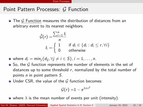
Point Pattern Processes: G Function

The G Function measures the distribution of distances from anarbitrary event to its nearest neighbors.

G(r) =

∑ni=1 Iin

Ii =

{1 if di ∈ {di : di ≤ r , ∀i}0 otherwise

where di = minj{dij ,∀j 6= i ∈ S}, i = 1, . . . , n.

So, the G function represents the number of elements in the set ofdistances up to some threshold r , normalized by the total number ofpoints n in point pattern S .

Under CSR, the value of the G function becomes:

G(r) =1− eλπr2

where λ is the mean number of events per unit (intensity).


Point Processes

Point Pattern Processes: G Function

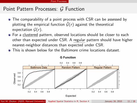
The comparability of a point process with CSR can be assessed byplotting the empirical function G(r) against the theoreticalexpectation G(r).For a clustered pattern, observed locations should be closer to eachother than expected under CSR. A regular pattern should have highernearest-neighbor distances than expected under CSR.This is shown below for the Baltimore crime locations dataset.

G Function

Expected

Observed

0.2

0.4

0.6

0.8

0.2 0.4 0.6 0.8

Baltimore Data

0.2 0.4 0.6 0.8

Random Pattern

0.2 0.4 0.6 0.8

Regular Pattern


Point Processes

Point Pattern Processes: F Function

The F Function measures the distribution of all distances from anarbitrary point k in the plane to the nearest observed event j .

F(r) =

∑mk=1 Ikm

Ik =

{1 if dk ∈ {dk : dk ≤ r , ∀k}0 otherwise

where dk = minj{dkj , ∀j ∈ S}, k = 1, . . . ,m, j = 1, . . . , n.

Under CSR, the expected value is also

F(r) =1− eλπr2


Point Processes

Point Pattern Processes: F Function

As before, we can plot the empirical function F(r) against itstheoretical expectation F(r).For a clustered pattern, observed locations j should be farther awayfrom random points k than expected under CSR. In a regular pattern,random locations should be closer to observed points.This is again shown below for the Baltimore crime locations dataset.

F Function

Expected

Observed

0.2

0.4

0.6

0.8

0.2 0.4 0.6 0.8

Baltimore Data

0.2 0.4 0.6 0.8

Random Pattern

0.2 0.4 0.6 0.8

Regular Pattern


Point Processes

Point Pattern Processes: Intensity

For an HPP point process, intensity is a constant λ(x) = λ = n|A| ,

where n is the number of points observed in region A, and |A| is thearea of region A.

For an IPP point process, intensity is non-constant and can beestimated non-parametrically with kernel smoothing (Diggle 1985,Berman and Diggle 1989, Bivand et. al. 2008).


Point Processes

Point Pattern Processes: Kernel Density

The kernel density estimator is:

λ(x) =1

h2

n∑i=1

κ(||x−xi ||

h

)q(||x ||)

where xi ∈ {x1, . . . , xn is an observed point, h is the bandwidth,q(||x ||) is a border correction to compensate for observations missingdue to edge effects, and κ(u) is a bivariate and symmetrical kernelfunction.

R currently implements a two-dimensional quartic kernel function:

κ(u) =

{3π (1− ||u||2)2 if u ∈ (−1, 1)0 otherwise

where ||u||2 = u21 + u22 is the squared norm of point u = (u1, u2)


Point Processes


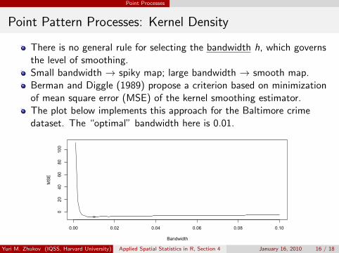
There is no general rule for selecting the bandwidth h, which governsthe level of smoothing.Small bandwidth → spiky map; large bandwidth → smooth map.Berman and Diggle (1989) propose a criterion based on minimizationof mean square error (MSE) of the kernel smoothing estimator.The plot below implements this approach for the Baltimore crimedataset. The “optimal” bandwidth here is 0.01.

0.00 0.02 0.04 0.06 0.08 0.10

020

4060

80100

Bandwidth

MSE


Point Processes


The plot below shows kernel density estimates for the Baltimore crimelocations at different values of the bandwidth h.

Lighter values indicate greater intensity of the point process.

Clearly, different bandwidths tell very different stories about thespatial intensity of crime in Baltimore...


Point Processes

Examples in R

Switch to R tutorial script. Section 4.


applied spatial statistics in r, section 4zhukov/spatial4.pdf · 2 spatial data and basic...

Documents