applied solid mechanics () - peter howell
DESCRIPTION
Good book for Solid MechanicsTRANSCRIPT


This page intentionally left blank
A P P L I E D S O L I D M E C H A N I C S
Much of the world around us, both natural and man-made, is built from and held
together by solid materials. Understanding how they behave is the task of solid
mechanics, which can in turn be applied to a wide range of areas from earthquake
mechanics and the construction industry to biomechanics. The variety of materials
(such as metals, rocks, glasses, sand, flesh and bone) and their properties (such as
porosity, viscosity, elasticity, plasticity) are reflected by the concepts and techniques
needed to understand them, which are a rich mixture of mathematics, physics, ex-
periment and intuition. These are all brought to bear in this distinctive book, which
is based on years of experience in research and teaching. Theory is related to
practical applications, where surprising phenomena occur and where innovative
mathematical methods are needed to understand features such as fracture. Starting
from the very simplest situations, based on elementary observations in engineer-
ing and physics, models of increasing sophistication are derived and applied. The
emphasis is on problem solving and on building an intuitive understanding, rather
than on a technical presentation of theoretical topics. The text is complemented by
over 100 carefully chosen exercises, and the minimal prerequisites make it an ideal
companion for mathematics students taking advanced courses, for those undertak-
ing research in the area or for those working in other disciplines in which solid
mechanics plays a crucial role.

Cambridge Texts in Applied Mathematics
Editorial Board
Mark Ablowitz, University of Colorado, BoulderS. Davis, Northwestern UniversityE. J. Hinch, University of CambridgeArieh Iserles, University of CambridgeJohn Ockendon, University of OxfordPeter Olver, University of Minnesota

APPLIED SOLID MECHANICS
P E T E R H O W E L LUniversity of Oxford
G R E G O R Y K O Z Y R E F FFonds de la Recherche Scientifique—FNRS
and Universite Libre de Bruxelles
J O H N O C K E N D O NUniversity of Oxford

CAMBRIDGE UNIVERSITY PRESS
Cambridge, New York, Melbourne, Madrid, Cape Town, Singapore, São Paulo
Cambridge University Press
The Edinburgh Building, Cambridge CB2 8RU, UK
First published in print format
ISBN-13 978-0-521-85489-4
ISBN-13 978-0-521-67109-5
ISBN-13 978-0-511-50639-0
© P. D. Howell, G. Kozyreff and J. R. Ockendon 2009
2008
Information on this title: www.cambridge.org/9780521854894
This publication is in copyright. Subject to statutory exception and to the
provision of relevant collective licensing agreements, no reproduction of any part
may take place without the written permission of Cambridge University Press.
Cambridge University Press has no responsibility for the persistence or accuracy
of urls for external or third-party internet websites referred to in this publication,
and does not guarantee that any content on such websites is, or will remain,
accurate or appropriate.
Published in the United States of America by Cambridge University Press, New York
www.cambridge.org
paperback
eBook (EBL)
hardback

Contents
List of illustrations page viiiPrologue xiii
Modelling solids 11.1 Introduction 11.2 Hooke’s law 21.3 Lagrangian and Eulerian coordinates 31.4 Strain 41.5 Stress 71.6 Conservation of momentum 101.7 Linear elasticity 111.8 The incompressibility approximation 131.9 Energy 141.10 Boundary conditions and well-posedness 161.11 Coordinate systems 19Exercises 24
Linear elastostatics 282.1 Introduction 282.2 Linear displacements 292.3 Antiplane strain 372.4 Torsion 392.5 Multiply-connected domains 422.6 Plane strain 472.7 Compatibility 682.8 Generalised stress functions 702.9 Singular solutions in elastostatics 822.10 Concluding remark 93Exercises 93
v

vi Contents
Linear elastodynamics 1033.1 Introduction 1033.2 Normal modes and plane waves 1043.3 Dynamic stress functions 1213.4 Waves in cylinders and spheres 1243.5 Initial-value problems 1323.6 Moving singularities 1383.7 Concluding remarks 143Exercises 143
Approximate theories 1504.1 Introduction 1504.2 Longitudinal displacement of a bar 1514.3 Transverse displacements of a string 1524.4 Transverse displacements of a beam 1534.5 Linear rod theory 1584.6 Linear plate theory 1624.7 Von Karman plate theory 1724.8 Weakly curved shell theory 1774.9 Nonlinear beam theory 1874.10 Nonlinear rod theory 1954.11 Geometrically nonlinear wave propagation 1984.12 Concluding remarks 204Exercises 205
Nonlinear elasticity 2155.1 Introduction 2155.2 Stress and strain revisited 2165.3 The constitutive relation 2215.4 Examples 2335.5 Concluding remarks 239Exercises 239
Asymptotic analysis 2456.1 Introduction 2456.2 Antiplane strain in a thin plate 2466.3 The linear plate equation 2486.4 Boundary conditions and Saint-Venant’s principle 2536.5 The von Karman plate equations 2616.6 The Euler–Bernoulli plate equations 2676.7 The linear rod equations 2736.8 Linear shell theory 278

This page intentionally left blank

Contents vii
6.9 Concluding remarks 282Exercises 283
Fracture and contact 2877.1 Introduction 2877.2 Static brittle fracture 2887.3 Contact 3097.4 Concluding remarks 320Exercises 321
Plasticity 3288.1 Introduction 3288.2 Models for granular material 3308.3 Dislocation theory 3378.4 Perfect plasticity theory for metals 3448.5 Kinematics 3588.6 Conservation of momentum 3608.7 Conservation of energy 3608.8 The flow rule 3628.9 Simultaneous elasticity and plasticity 3648.10 Examples 3658.11 Concluding remarks 370Exercises 372
More general theories 3789.1 Introduction 3789.2 Viscoelasticity 3799.3 Thermoelasticity 3889.4 Composite materials and homogenisation 3919.5 Poroelasticity 4089.6 Anisotropy 4139.7 Concluding remarks 417Exercises 417
Epilogue 426
Appendix Orthogonal curvilinear coordinates 428References 440Index 442

Illustrations
1.1 A reference tetrahedron. page 81.2 The forces acting on a small two-dimensional element. 91.3 A small pill-box-shaped region at the boundary between two elastic
solids. 181.4 Forces acting on a polar element of solid. 221.5 A system of masses connected by springs. 252.1 A unit cube undergoing (a) uniform expansion, (b) one-dimensional
shear, (c) uniaxial stretching. 302.2 A uniform bar being stretched under a tensile force. 322.3 A paper model with negative Poisson’s ratio. 332.4 A strained plate. 342.5 A bar in a state of antiplane strain. 382.6 A twisted bar. 392.7 A uniform tubular torsion bar. 432.8 The cross-section of (a) a circular cylindrical tube; (b) a cut tube. 442.9 The unit normal and tangent to the boundary of a plane region. 492.10 A plane annulus being inflated by an internal pressure. 532.11 A plane rectangular region subject to tangential tractions on its faces. 572.12 The tractions applied to the edge of a semi-infinite strip. 592.13 The surface displacement of a half-space and corresponding surface
pressure. 652.14 A family of functions δε(x) that approach a delta-function as ε → 0. 832.15 Contours of the maximum shear stress created by a point force acting
at the origin. 852.16 Four point forces. 913.1 Plots of the first three Bessel functions. 1083.2 A P -wave reflecting from a rigid boundary. 1163.3 A layered elastic medium. 1173.4 Dispersion relation for symmetric and antisymmetric Love waves. 1203.5 Illustration of flexural waves. 1283.6 The one-dimensional fundamental solution. 1343.7 The two-dimensional fundamental solution. 135
viii

List of illustrations ix
3.8 The cone x2 + y2 = c2t2 tangent to the plane k1x + k2y = ωt. 1383.9 The two-sheeted characteristic cone for the Navier equation. 1383.10 The response of a string to a point force moving at speed V . 1393.11 Wave-fronts generated by a moving force on an elastic membrane. 1413.12 P -wave- and S -wave-fronts generated by a point force moving at speed
V in plane strain. 1423.13 Group velocity versus wave-number for symmetric and antisymmetric
Love waves. 1464.1 The forces acting on a small length of a uniform bar. 1514.2 The forces acting on a small length of an elastic string. 1534.3 The forces and moments acting on a small segment of an elastic beam. 1544.4 The end of a beam under clamped, simply supported and free conditions.1554.5 The first three buckling modes of a clamped elastic beam. 1574.6 The internal force components in a thin elastic rod. 1594.7 Cross-section through a rod showing the bending moment components. 1594.8 Examples of cross-sections in the (y, z)-plane and their bending
stiffnesses. 1614.9 The forces acting on a small section of an elastic plate. 1634.10 The bending moments acting on a section of an elastic plate. 1644.11 The displacement of a simply supported rectangular plate sagging
under gravity. 1694.12 (a) A cylinder, (b) a cone, (c) another developable surface, (d) a
hyperboloid. 1754.13 Typical surface shapes with (a) zero, (b) negative and (c) positive
Gauss 1794.14 Deformations of a cylindrical shell. 1844.15 Deformations of an anticlastic shell. 1854.16 Deformations of a synclastic shell. 1864.17 A beam (a) before and (b) after bending; (c) a close-up of the
displacement field. 1874.18 (a) The forces and moments acting on a small segment of a beam.
(b) The sign convention for the forces at the ends of the beam. 1884.19 (a) Final angle of a diving board versus applied force parameter.
(b) Deflection of a diving board for various values of the force parameter.1914.20 (a) Response diagram of the amplitude of the linearised solution for a
buckling beam versus the force parameter. (b) Corresponding responseof the weakly nonlinear solution. 193
4.21 (a) Pitchfork bifurcation diagram of leading-order amplitude versusforcing parameter. (b) The corresponding diagram when asymmetry isintroduced. 195
4.22 A system of pendulums attached to a twisting rubber band. 1994.23 A kink propagating along a series of pendulums attached to a rod. 2004.24 Travelling wave solution of the nonlinear beam equations. 2014.25 A beam clamped near the edge of a table. 2064.26 A beam supported at two points. 207
ian curvature.
4.27 The first three buckling modes of a vertically clamped beam. 213

x List of illustrations
5.1 The deformation of a small scalene cylinder. 2185.2 Typical force–strain graphs for uniaxial tests on various materials. 2335.3 A square membrane subject to an isotropic tensile force. 2345.4 Response diagrams for a biaxially-loaded incompressible sheet of
Mooney–Rivlin material. 2355.5 Scaled pressure inside a balloon as a function of the stretch for various
values of the Mooney–Rivlin parameter. 2365.6 Gas pressure inside a cavity as a function of inflation coefficient for
various values of the Mooney–Rivlin parameter. 2386.1 The edge of a plate subject to tractions. 2546.2 The geometry of a deformed two-dimensional plate. 2697.1 Definition sketch of a thin crack. 2887.2 Definition sketch for contact between two solids. 2887.3 (a) A Mode III crack. (b) A cross-section in the (x, y)-plane. 2907.4 Definition sketch for the function
√z2 − c2 . 292
7.5 Displacement field for a Mode III crack. 2937.6 (a) A planar Mode II crack. (b) The regularised problem of a thin
elliptical crack. 2977.7 Contour plot of the maximum shear stress around a Mode II crack. 3017.8 The displacement of a Mode II crack under increasing shear stress. 3037.9 A Mode I crack. 3047.10 Contour plot of the maximum shear stress around a Mode I crack. 3067.11 The displacement of a Mode I crack under increasing normal stress. 3077.12 Solution for the contact between a string and a level surface. 3107.13 Three candidate solutions for a contact problem. 3117.14 The contact between a beam and a horizontal surface under a uniform
pressure. 3147.15 Contact between a rigid body and an elastic half-space. 3177.16 The penetration of a quadratic punch into an elastic half-space. 3197.17 A flexible ruler flattened against a table. 3267.18 A wave travelling along a rope on the ground. 3268.1 A typical stress–strain relationship for a plastic material. 3298.2 The stress–strain relationship for a perfectly plastic material. 3308.3 The forces acting on a particle at the surface of a granular material. 3318.4 The normal force and frictional force acting on a surface element inside
a granular material. 3328.5 The Mohr circle. 3338.6 The triaxial stress factor versus angle of friction. 3368.7 An antiplane cut-and-weld operation. 3398.8 The displacement field in an edge dislocation. 3408.9 An edge dislocation in a square crystal lattice. 3418.10 A moving edge dislocation. 3428.11 The normalised torque versus twist applied to an elastic-plastic
cylindrical bar. 3478.12 The normalised torque versus twist applied to an elastic-plastic
cylindrical bar, showing the recovery phase. 348

List of illustrations xi
8.13 The free-boundary problem for an elastic-perfectly plastic torsion bar. 3498.14 Residual shear stress in a gun barrel versus radial distance for different
values of the maximum internal pressurisation. 3528.15 The Tresca yield surface. 3558.16 The von Mises yield surface. 3568.17 The Coulomb yield surface. 3588.18 Luders bands in a thin sheet of metal. 3698.19 The Mohr surface for three-dimensional granular flow. 3738.20 The normalised torque versus twist applied to an elastic-plastic
cylindrical bar undergoing a loading cycle. 3759.1 (a) A spring; (b) a dashpot; (c) a spring and dashpot connected in
parallel; (d) a spring and dashpot connected in series. 3809.2 (a) Applied tension as a function of time. (b) Resultant displacement
of a linear elastic spring. (c) Resultant displacement of a linear dashpot.3819.3 Displacement of a Voigt element due to the applied tension shown in
Figure 9.2(a). 3829.4 Displacement of a Maxwell element due to the applied tension shown
in Figure 9.2(a). 3839.5 (a) The variation of Young’s modulus with position in a bar. (b) The
corresponding longitudinal displacement. 3929.6 (a) The variation of Young’s modulus with position in a bar. (b) The
corresponding longitudinal displacement. 3959.7 A periodic microstructured shear modulus. 3969.8 A symmetric, piecewise constant shear modulus distribution. 4009.9 Some modulus distributions that are antisymmetric about the diago-
nals of a square. 4029.10 Dimensionless wavenumber versus the Young’s modulus non-uniformity
parameter. 4079.11 The one-dimensional squeezing of a sponge. 4119.12 Dimensionless stress applied to a sponge versus dimensionless time for
different values of the Peclet number. 4129.13 A Jeffreys viscoelastic element. 4189.14 A system of masses connected by springs and dashpots in parallel. 4189.15 A system of masses connected by springs and dashpots in series. 4199.16 Dimensionless wavenumber versus Young’s modulus contrast for a
piecewise uniform bar. 424A1.1 A small reference box. 432A1.2 Cylindrical polar coordinates. 437A1.3 Spherical polar coordinates. 438

Prologue
Although solid mechanics is a vitally important branch of applied mechan-ics, it is often less popular, at least among students, than its close relative,fluid mechanics. Several reasons can be advanced for this disparity, such asthe prevalence of tensors in models for solids or the especial difficulty of han-dling nonlinearity. Perhaps the most daunting prospect for the student is themultitude of different behaviours that can occur and cause elementary theo-ries of elasticity to become irrelevant in practice. Examples include fracture,buckling and plasticity, and these pose intellectual challenges in solid me-chanics that are every bit as fascinating as concepts like flight, shock wavesand turbulence in fluid dynamics. Our principal objective in this book is todemonstrate this fact to undergraduate and beginning graduate students.
We aim to give the subject as wide an accessibility as possible to math-ematically-minded students and to emphasise the interesting mathematicalissues that it raises. We do this by relating the theory to practical applica-tions where surprising phenomena occur and where innovative mathematicalmethods are needed.
Our layout is essentially pragmatic. Although more advanced texts in solidmechanics often begin with quite general theories founded on basic mechan-ical and thermodynamic principles, we start from the very simplest models,based on elementary observations in engineering and physics, and build ourway towards models that are the basis for current applied research in solidmechanics. Hence, we begin by deriving the basic Navier equations of linearelasticity, before illustrating the mathematical techniques that allow theseequations to be solved in many different practically relevant situations, bothstatic and dynamic. We then proceed to describe some approximate theoriesfor the elastic deformation of thin solids, namely bars, strings, beams, rods,plates and shells. We soon discover that many everyday phenomena, such asthe buckling of a beam under a compressive load, cannot be fully described
xiii

xiv Prologue
using linear theories. We therefore give a brief exposition of the general the-ory of nonlinear elasticity, and then show how formal asymptotic methodsallow simplified linear and weakly nonlinear models to be systematically de-duced. Although we regard such asymptotic techniques as invaluable to anyapplied mathematician, these last two topics may both be omitted on a firstreading without loss of continuity. We go on to present simple models forfracture and contact, comparing and contrasting these apparently similarphenomena. Next, we show how plasticity theory can be used to describesituations where a solid yields under a sufficiently high stress. Finally, weshow how elasticity theory may be generalised to include further physical ef-fects, such as thermal stresses, viscoelasticity and porosity. These “combinedfields” of solid mechanics are increasingly finding applications in industrialand medical processes, and pose ever more elaborate modelling questions.
Despite the breadth of the models and relevant techniques that will emergein this book, we will usually try to present the theoretical developmentsab initio. Nonetheless, the book is very far from being self-contained. Anystudent who aspires to becoming a solid mechanics specialist will have todelve further into the literature, and we will provide references to help withthis.
We assume only that the reader has a reasonable familiarity with thecalculus of several variables. Fluency with the more advanced techniquesrequired for Chapters 6 and 7, in particular, will readily be acquired bya student who works through the exercises in the early Chapters, espe-cially those cited in the text. Indeed, we firmly believe that solid mechanicsprovides a wonderful arena in which to build an understanding of such im-portant mathematical areas as linear algebra, partial differential equations,complex variable theory, differential geometry and the calculus of variations.Our hope is that, having read this book, a student should be able to confrontany practical problem that may be encountered in everyday solid mechanicswith at least some idea of the basic mathematical modelling that will berequired.
During the writing of this book, we received a great deal of help and inspi-ration as a result of discussions with David Allwright, Jon Chapman, SamHowison, L. Mahadevan, Roman Novokshanov and Domingo Salazar, as wellas many other colleagues and students too numerous to thank individually.We would like to express our particular gratitude to Gareth Jones, HilaryOckendon and Tom Witelski who gave invaluable advice on draft Chapters.We are also indebted to David Tranah and his colleagues at CambridgeUniversity Press for helping to make this book a reality.

1
Modelling solids
1.1 Introduction
In everyday life we regularly encounter physical phenomena that apparentlyvary continuously in space and time. Examples are the bending of a paperclip, the flow of water or the propagation of sound or light waves. Such phe-nomena can be described mathematically, to lowest order, by a continuummodel, and this book will be concerned with that class of continuum modelsthat describes solids. Hence, at least to begin with, we will avoid all consid-eration of the “atomistic” structure of solids, even though these ideas leadto great practical insight and also to some beautiful mathematics. Whenwe refer to a solid “particle”, we will be thinking of a very small region ofmatter but one whose dimension is nonetheless much greater than an atomicspacing.
For our purposes, the diagnostic feature of a solid is the way in which itresponds to an applied system of forces and moments. There is no hard-and-fast rule about this but, for most of this book, we will say that a continuum isa solid when the response consists of displacements distributed through thematerial. In other words, the material starts at some reference state, fromwhich it is displaced by a distance that depends on the applied forces. This isin contrast with a fluid, which has no special rest state and responds to forcesvia a velocity distribution. Our modelling philosophy is straightforward. Wetake the most fundamental pieces of experimental evidence, for exampleHooke’s law, and use mathematical ideas to combine this evidence withthe basic laws of mechanics to construct a model that describes the elasticdeformation of a continuous solid. Following this simple approach, we willfind that we can construct solid mechanics theories for phenomena as diverseas earthquakes, ultrasonic testing and the buckling of railway tracks.
1
2 Modelling solids
By basing our theory on Hooke’s law, the simplest model of elasticity,for small enough forces and displacements, we will first be led to a systemof differential equations that is both linear, and therefore mathematicallytractable, and reversible for time-dependent problems. By this we meanthat, when forces and moments are applied and then removed, the systemeventually returns to its original state without any significant energy beinglost, i.e. the system is not dissipative.
Reversibility may apply even when the forces and displacements are solarge that the problem ceases to be linear; a rubber band, for example,can undergo large displacements and still return to its initial state. How-ever, nonlinear elasticity encompasses some striking new behaviours notpredicted by linear theory, including the possibility of multiple steady statesand buckling. For many materials, experimental evidence reveals that evenmore dramatic changes can take place as the load increases, the most strik-ing phenomenon being that of fracture under extreme stress. On the otherhand, as can be seen by simply bending a metal paper clip, irreversibilitycan readily occur and this is associated with plastic flow that is significantlydissipative. In this situation, the solid takes on some of the attributes of afluid, but the model for its flow is quite different from that for, say, water.
Practical solid mechanics encompasses not only all the phenomena men-tioned above but also the effects of elasticity when combined with heattransfer (leading to thermoelasticity) and with genuine fluid effects, in caseswhere the material flows even in the absence of large applied forces (leadingto viscoelasticity) or when the material is porous (leading to poroelastic-ity). We will defer consideration of all these combined fields until the finalchapter.
1.2 Hooke’s law
Robert Hooke (1678) wrote
“it is . . . evident that the rule or law of nature in every springing body is that theforce or power thereof to restore itself to its natural position is always proportionateto the distance or space it is removed therefrom, whether it be by rarefaction, orseparation of its parts the one from the other, or by condensation, or crowding ofthose parts nearer together.”
Hooke’s observation is exemplified by a simple high-school physics experi-ment in which a tensile force T is applied to a spring whose natural lengthis L. Hooke’s law states that the resulting extension of the spring is propor-tional to T : if the new length of the spring is , then
T = k( − L), (1.2.1)
where the constant of proportionality k is called the spring constant.

1.3 Lagrangian and Eulerian coordinates 3
Hooke devised his law while designing clock springs, but noted that itappears to apply to all “springy bodies whatsoever, whether metal, wood,stones, baked earths, hair, horns, silk, bones, sinews, glass and the like.” Inpractice, it is commonly observed that k scales with 1/L; that is, everythingelse being equal, a sample that is initially twice as long will stretch twiceas far under the same force. It is therefore sensible to write (1.2.1) in theform
T = k′ − L
L, (1.2.2)
where k′ is the elastic modulus of the spring, which will be defined morerigorously in Chapter 2. The dimensionless quantity ( − L)/L, measuringthe extension relative to the initial length, is called the strain.
Equation (1.2.2) is the simplest example of the all-important constitutivelaw relating the force to displacement. As shown in Exercise 1.3, it is possibleto construct a one-dimensional continuum model for an elastic solid fromthis law, but, to generalise it to a three-dimensional continuum, we first needto generalise the concepts of strain and tension.
1.3 Lagrangian and Eulerian coordinates
Suppose that a three-dimensional solid starts, at time t = 0, in its reststate, or reference state, in which no macroscopic forces exist in the solidor on its boundary. Under the action of any subsequently applied forcesand moments, the solid will be deformed such that, at some later time t, a“particle” in the solid whose initial position was the point X is displacedto the point x (X, t). This is a Lagrangian description of the continuum: ifthe independent variable X is held fixed as t increases, then x(X, t) labelsa material particle. In the alternative Eulerian approach, we consider thematerial point which currently occupies position x at time t, and label itsinitial position by X(x, t). In short, the Eulerian coordinate x is fixed inspace, while the Lagrangian coordinate X is fixed in the material.
The displacement u(X, t) is defined in the obvious way to be the differencebetween the current and initial positions of a particle, that is
u(X, t) = x(X, t) − X. (1.3.1)
Many basic problems in solid mechanics amount to determining the dis-placement field u corresponding to a given system of applied forces.
The mathematical consequence of our statement that the solid is a con-tinuum is that there must be a smooth one-to-one relationship between X
and x, i.e. between any particle’s initial position and its current position.
4 Modelling solids
This will be the case provided the Jacobian of the transformation from X
to x is bounded away from zero:
0 < J < ∞, where J = det(
∂xi
∂Xj
). (1.3.2)
The physical significance of J is that it measures the change in a smallvolume compared with its initial volume:
dx1dx2dx3 = J dX1dX2dX3, or dx = J dX (1.3.3)
as shorthand. The positivity of J means that we exclude the possibility thatthe solid turns itself inside-out.
We can use (1.3.3) to derive a kinematic equation representing conserva-tion of mass. Consider a moving volume V (t) that is always bounded bythe same solid particles. Its mass at time t is given, in terms of the densityρ(X, t), by
M(t) =∫∫∫
V (t)ρ dx =
∫∫∫V (0)
ρJ dX. (1.3.4)
Since V (t) designates a fixed set of material points, M(t) must be a constant,namely its initial value M(0):∫∫∫
V (0)ρJ dX = M(t) = M(0) =
∫∫∫V (0)
ρ0 dX, (1.3.5)
where ρ0 is the density in the rest state. Since V is arbitrary, we deduce that
ρJ = ρ0. (1.3.6)
Hence, we can calculate the density at any time t in terms of ρ0 and thedisplacement field. The initial density ρ0 is usually taken as constant, but(1.3.6) also applies if ρ0 = ρ0(X).
1.4 Strain
To generalise the concept of strain introduced in Section 1.2, we consider thedeformation of a small line segment joining two neighbouring particles withinitial positions X and X + δX. At some later time, the solid deforms suchthat the particles are displaced to X +u(X, t) and X + δX +u(X + δX, t)respectively. Thus we can use Taylor’s theorem to show that the line element
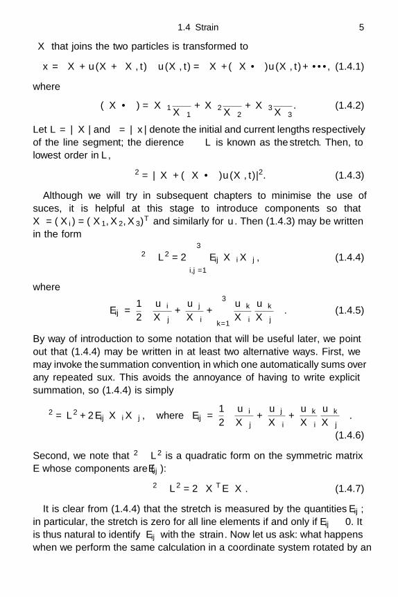
1.4 Strain 5
δX that joins the two particles is transformed to
δx = δX +u(X + δX, t)−u(X, t) = δX +(δX ·∇)u(X, t)+ · · · , (1.4.1)
where
(δX · ∇) = δX1∂
∂X1+ δX2
∂
∂X2+ δX3
∂
∂X3. (1.4.2)
Let L = |δX| and = |δx| denote the initial and current lengths respectivelyof the line segment; the difference − L is known as the stretch. Then, tolowest order in L,
2 = |δX + (δX · ∇)u(X, t)|2. (1.4.3)
Although we will try in subsequent chapters to minimise the use ofsuffices, it is helpful at this stage to introduce components so thatX = (Xi) = (X1, X2, X3)T and similarly for u. Then (1.4.3) may be writtenin the form
2 − L2 = 23∑
i,j=1
Eij δXiδXj, (1.4.4)
where
Eij =12
(∂ui
∂Xj+
∂uj
∂Xi+
3∑k=1
∂uk
∂Xi
∂uk
∂Xj
). (1.4.5)
By way of introduction to some notation that will be useful later, we pointout that (1.4.4) may be written in at least two alternative ways. First, wemay invoke the summation convention, in which one automatically sums overany repeated suffix. This avoids the annoyance of having to write explicitsummation, so (1.4.4) is simply
2 = L2 + 2Eij δXiδXj, where Eij =12
(∂ui
∂Xj+
∂uj
∂Xi+
∂uk
∂Xi
∂uk
∂Xj
).
(1.4.6)
Second, we note that 2 − L2 is a quadratic form on the symmetric matrixE whose components are (Eij):
2 − L2 = 2 δXTE δX. (1.4.7)
It is clear from (1.4.4) that the stretch is measured by the quantities Eij ;in particular, the stretch is zero for all line elements if and only if Eij ≡ 0. Itis thus natural to identify Eij with the strain. Now let us ask: “what happenswhen we perform the same calculation in a coordinate system rotated by an

6 Modelling solids
orthogonal matrix P = (pij)?” Intuitively, we might expect the strain to beinvariant under such a rotation, and we can verify that this is so as follows.
The vectors X and u are transformed to X ′ and u′ in the new coordinatesystem, where
X ′ = PX, u′ = Pu. (1.4.8)
Since P is orthogonal, (1.4.8) may be inverted to give X = PTX ′. Alterna-tively, using suffix notation, we have
Xβ = pjβX ′j , u′
i = piαuα. (1.4.9)
The strain in the new coordinate system is denoted by
E ′ij =
12
(∂u′
i
∂X ′j
+∂u′
j
∂X ′i
+∂u′
k
∂X ′i
∂u′k
∂X ′j
), (1.4.10)
which may be manipulated using the chain rule, as shown in Exercise 1.4,to give
E ′ij = piαpjβEαβ. (1.4.11)
In matrix notation, (1.4.11) takes the form
E ′ = PEPT, (1.4.12)
so the 3 × 3 symmetric array (Eij) transforms exactly like a matrix repre-senting a linear transformation of the vector space R3. Arrays that obey thetransformation law (1.4.11) are called second-rank Cartesian tensors, andE = (Eij) is therefore called the strain tensor.†
Almost as important as the fact that E is a tensor is the fact that itcan vanish without u vanishing. More precisely, if we consider a rigid-bodytranslation and rotation
u = c + (Q − I)X, (1.4.13)
where I is the identity matrix while the vector c and orthogonal matrixQ are constant, then E is identically zero. This result follows directly fromsubstituting (1.4.13) into (1.4.6) and using the fact that QQT = I, andconfirms our intuition that a rigid-body motion induces no deformation.
†The word “tensor” as used here is effectively synonymous with “matrix”, but it is easy togeneralise (1.4.11) to a tensor with any number of indices. A vector, for example, is a tensorwith just one index.

1.5 Stress 7
1.5 Stress
In the absence of any volumetric (e.g. gravitational or electromagnetic) ef-fects, a force can only be transmitted to a solid by being applied to itsboundary. It is, therefore, natural to consider the force per unit area orstress applied at that boundary. To do so, we now analyse an infinitesimalsurface element, whose area and unit normal are da and n respectively. If itis contained within a stressed medium, then the material on (say) the sideinto which n points will exert a force df on the element. (By Newton’s thirdlaw, the material on the other side will also exert a force equal to −df .) Inthe expectation that the force should be proportional to the area da, wewrite
df = σ da, (1.5.1)
where σ is called the traction or stress acting on the element.Perhaps the most familiar example is that of an inviscid fluid, in which
the stress is related to the pressure p by
σ = −pn. (1.5.2)
This expression implies that (i) the stress acts only in a direction normalto the surface element, (ii) the magnitude of the stress (i.e. p) is indepen-dent of the direction of n. In an elastic solid, neither of these simplifyingassumptions holds; we must allow for stress which acts in both tangentialand normal directions and whose magnitude depends on the orientation ofthe surface element.
First consider a surface element whose normal points in the x1-direction,and denote the stress acting on such an element by τ 1 = (τ11, τ21, τ31)T. Bydoing the same for elements with normals in the x2- and x3-directions, wegenerate three vectors τ j (j = 1, 2, 3), each representing the stress actingon an element normal to the xj -direction. In total, therefore, we obtain ninescalars τij (i, j = 1, 2, 3), where τij is the i-component of τ j , that is
τ j = τijei, (1.5.3)
where ei is the unit vector in the xi-direction.The scalars τij may be used to determine the stress on an arbitrary surface
element by considering the tetrahedron shown in Figure 1.1. Here ai denotesthe area of the face orthogonal to the xi-axis. The fourth face has areaa =
√a2
1 + a22 + a2
3; in fact if this face has unit normal n as shown, withcomponents (ni), then it is an elementary exercise in trigonometry to showthat ai = ani.

8 Modelling solids
a2
a3
x1
x3
x2
n
a1
Fig. 1.1 A reference tetrahedron; ai is the area of the face orthogonal to the xi-axis.
The outward normal to the face with area a1 is in the negative x1-directionand the force on this face is thus −a1τ 1. Similar expressions hold for thefaces with areas a2 and a3. Hence, if the stress on the fourth face is denotedby σ, then the total force on the tetrahedron is
f = aσ − ajτ j . (1.5.4)
When we substitute for aj and τ j , we find that the components of f aregiven by
fi = a (σi − τijnj) . (1.5.5)
Now we shrink the tetrahedron to zero volume. Since the area a scaleswith 2, where is a typical edge length, while the volume is proportionalto 3, if we apply Newton’s second law and insist that the acceleration befinite, we see that f/a must tend to zero as → 0.† Hence we deduce an
†Readers of a sensitive disposition may be slightly perturbed by our glibly letting the dimensionalvariable tend to zero: if is reduced indefinitely then we will eventually reach an atomic scaleon which the solid can no longer be treated as a continuum. We reassure such readers that(1.5.6) can be more rigorously justified provided the macroscopic dimensions of the solid arelarge compared to any atomistic length-scale.
1.5 Stress 9
Gτ11
τ11
τ22
τ21
τ22
τ12
τ12
τ21
x2
x1
δx2
δx1
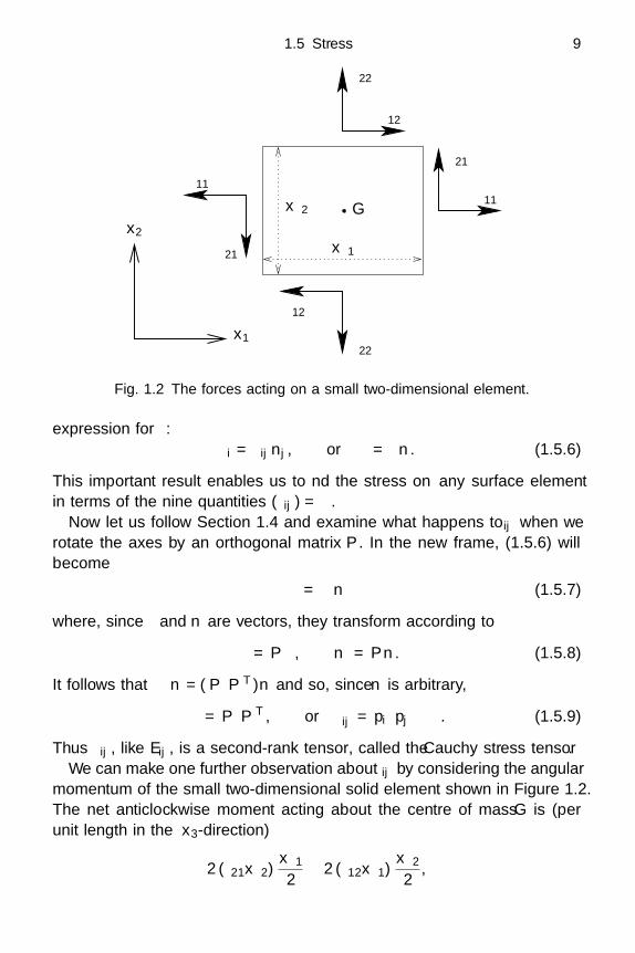
Fig. 1.2 The forces acting on a small two-dimensional element.
expression for σ:σi = τijnj , or σ = τn. (1.5.6)
This important result enables us to find the stress on any surface elementin terms of the nine quantities (τij) = τ .
Now let us follow Section 1.4 and examine what happens to τij when werotate the axes by an orthogonal matrix P . In the new frame, (1.5.6) willbecome
σ′ = τ ′n′ (1.5.7)
where, since σ and n are vectors, they transform according to
σ′ = Pσ, n′ = Pn. (1.5.8)
It follows that τ ′n = (PτPT)n and so, since n is arbitrary,
τ ′ = PτPT, or τ ′ij = piαpjβταβ. (1.5.9)
Thus τij , like Eij , is a second-rank tensor, called the Cauchy stress tensor.We can make one further observation about τij by considering the angular
momentum of the small two-dimensional solid element shown in Figure 1.2.The net anticlockwise moment acting about the centre of mass G is (perunit length in the x3-direction)
2 (τ21δx2)δx1
2− 2 (τ12δx1)
δx2
2,
10 Modelling solids
where τ21 and τ12 are evaluated at G to lowest order. By letting the rectangleshrink to zero (see again the footnote on page 8), and insisting that theangular acceleration be finite, we deduce that τ12 = τ21. This argument canbe generalised to three dimensions (see Exercise 1.5) and it shows that
τij ≡ τji (1.5.10)
for all i and j, i.e. that τij , like Eij , is a symmetric tensor.
1.6 Conservation of momentum
Now we derive the basic governing equation of solid mechanics by apply-ing Newton’s second law to a material volume V (t) that moves with thedeforming solid:
ddt
∫∫∫V (t)
∂ui
∂tρ dx =
∫∫∫V (t)
giρ dx +∫∫
∂V (t)τijnj da. (1.6.1)
The terms in (1.6.1) represent successively the rate of change of momentumof the material in V (t), the force due to an external body force g, such asgravity, and the traction exerted on the boundary of V , whose unit normalis n, by the material around it. We differentiate under the integral (usingthe fact that ρ dx = ρ0 dX is independent of t) and apply the divergencetheorem to the final term to obtain∫∫∫
V (t)
∂2ui
∂t2ρ dx =
∫∫∫V (t)
giρ dx +∫∫∫
V (t)
∂τij
∂xjdx. (1.6.2)
Assuming each integrand is continuous, and using the fact that V (t) is ar-bitrary, we arrive at Cauchy’s momentum equation:
ρ∂2ui
∂t2= ρgi +
∂τij
∂xj. (1.6.3)
This may alternatively be written in vector form by adopting the followingnotation for the divergence of a tensor: we define the ith component of ∇ · τto be
(∇ · τ)i =∂τji
∂xj. (1.6.4)
Since τ is symmetric, we may thus write Cauchy’s equation as
ρ∂2u
∂t2= ρg + ∇ · τ. (1.6.5)
This equation applies to any continuous medium for which a displacementu and stress tensor τ can be defined. The distinction between solid, fluid
1.7 Linear elasticity 11
or some other continuum comes when we impose an empirical constitutiverelation between τ and u.
For solids, (1.6.5) already confronts us with a distinctive fundamentaldifficulty. The most obvious generalisation of Hooke’s law is to suppose thata linear relationship exists between the stress τ and the strain E . But wenow recall that E was defined in Section 1.4 in terms of the Lagrangianvariables X; indeed, the time derivative in (1.6.5) is taken in a Lagrangianframe, with X fixed. On the other hand, the stress tensor τ has been definedrelative to Eulerian coordinates and is differentiated in (1.6.5) with respectto the Eulerian variable x. It is not immediately clear, therefore, how thestress and strain, which are defined in different frames of reference, may beself-consistently related. We will postpone the full resolution of this difficultyuntil Chapter 5 and, for the present, restrict our attention to linear elasticityin which, as we shall see, the two frames are essentially identical.
1.7 Linear elasticity
The theory of linear elasticity follows from the assumption that the dis-placement u is small relative to any other length-scale. This assumptionallows the theory developed thus far to be simplified in several ways. First,it means that ∂ui/∂Xj is small for all i and j. Second, we note from (1.3.1)that x and X are equal to lowest order in u. Hence, if we only considerleading-order terms, there is no need to distinguish between the Eulerianand Lagrangian variables: we can simply replace X by x and ∂ui/∂Xj by∂ui/∂xj throughout. A corollary is that the Jacobian J is approximatelyequal to one, so (1.3.6) tells us that the density ρ is fixed, to leading order,at its initial value ρ0. Finally, we can use the smallness of ∂ui/∂xj to neglectthe quadratic term in (1.4.5) and hence obtain the linearised strain tensor
Eij ≈ eij =12
(∂ui
∂xj+
∂uj
∂xi
). (1.7.1)
Much of this book will be concerned with this approximation. Therefore,and with a slight abuse of notation, we will write E = (eij).
Remembering (1.4.13), we note that it is possible to approximate E by(1.7.1) even when u is not small compared with X, just as long as u is closeto a rigid-body translation and rotation. This situation is called geometricnonlinearity and we will encounter it frequently in Chapters 4 and 6. Itoccurs because Eij is identically zero for rigid-body motions of the solidgiven by (1.4.13); however eij does not vanish for such rigid-body motions,
12 Modelling solids
but rather for displacements of the form
u = c + ω× x, (1.7.2)
where c and ω are constant (see Exercise 1.6).Assuming the validity of (1.7.1), we can now generalise Hooke’s law by
postulating a linear relationship between the stress and strain tensors. Weassume that τ is zero when E is; in other words the stress is zero in thereference state. This is not the case for pre-stressed materials, and we willconsider some of the implications of so-called residual stress in Chapter 8.Even with this assumption, we apparently are led to the problem of defining81 material parameters Cijk (i, j, k, = 1, 2, 3) such that
τij = Cijkek. (1.7.3)
The symmetry of τij and eij only enables us to reduce the number ofunknowns to 36. This can be reduced to a more manageable number byassuming that the solid is isotropic, by which we mean that it behaves thesame way in all directions. This implies that Cijk must satisfy
Cijkpii′pjj′pkk′p′ ≡ Ci′j′k′′ (1.7.4)
for all orthogonal matrices P = (pij). It can be shown (see, for example,Ockendon & Ockendon, 1995, pp. 7–9) that this is sufficient to reduce thespecification of Cijk to just two scalar quantities λ and µ, such that
Cijk = λδijδk + 2µδikδj, (1.7.5)
where δij is the usual Kronecker delta, which represents the identity matrix;consequently,
τij = λ (ekk) δij + 2µeij . (1.7.6)
This relation can also be inverted to give the strain corresponding to a givenstress, that is
eij =12µ
(τij −
λ(τkk)(3λ + 2µ)
δij
). (1.7.7)
In Chapter 9 we will consider solids, such as wood or fibre-reinforced mate-rials, that are not isotropic, and for which (1.7.6) must be generalised.
The material parameters λ and µ are known as the Lame constants, and µ
is called the shear modulus.As we shall see in Chapter 2, λ and µ measure amaterial’s ability to resist elastic deformation. They have the units of pres-sure; typical values for a few familiar solid materials are given in Table 1.1.It will be observed that these values may be very large for relatively “hard”

1.8 The incompressibility approximation 13
λ (GPa) µ (GPa)
Cartilage 3 × 10⁻⁵ 9 × 10⁻⁵
Rubber 0.04 0.003Polystyrene 2.3 1.2Granite 10 30Glass 28 28Copper 86 37Steel 100 78Diamond 270 400
Table 1.1 Typical values of the Lame constants λ and µ for some everydaymaterials (1 GPa = 109 N m−2 = 104 atmospheres; a typical car tyre
pressure is two atmospheres).
materials, the significance being that tractions much less than these valueswill result in small deformations, so that linear elasticity is valid.
Now we substitute our linear constitutive relation (1.7.6) into the momen-tum equation (1.6.3) and replace X with x to obtain the Navier equation,also known as the Lame equation,
ρ∂2u
∂t2= ρg + (λ + µ) grad div u + µ∇2u. (1.7.8)
Recall that ρ does not vary to leading order, so (1.7.8) comprises threeequations for the three components of u. It may alternatively be written incomponent form
ρ∂2ui
∂t2= ρgi + (λ + µ)
∂2uj
∂xi∂xj+ µ
∂2ui
∂x2j
, (1.7.9)
where the final ∂x2j is treated as a repeated suffix, or
ρ∂2u
∂t2= ρg + (λ + 2µ) grad div u − µ curl curlu, (1.7.10)
where we have used the well-known vector identity
“del squared equals grad div minus curl curl.” (1.7.11)
1.8 The incompressibility approximation
There is an interesting and important class of materials that, although elas-tic, are virtually incompressible, so they may be sheared elastically but arehighly resistant to tension or compression. In linear elasticity, this amountsto saying that the Lame constant λ is much larger than the shear modulus µ.

14 Modelling solids
The values given in Table 1.1 show that rubber has this property, as do manybiomaterials such as muscle.
If a material is almost incompressible, we can set
λ
µ=
1ε, (1.8.1)
where ε is a small parameter. From (1.7.8), we expect that, in the limitε → 0, div u will be of order ε. Hence, if we define a scalar function p suchthat
pε = −µ
εdiv u, (1.8.2)
then pε will approach a finite limit p as ε → 0.When we now substitute (1.8.1) and (1.8.2) into the Navier equation
(1.7.8) and let ε → 0, we obtain
ρ∂2u
∂t2= ρg − ∇p + µ∇2u, (1.8.3a)
along with the limit of (1.8.2), that is
div u = 0. (1.8.3b)
The condition (1.8.3b) means that each material volume is conserved duringthe deformation, and it imposes an extra constraint on the Navier equation.The extra unknown p, representing the isotropic pressure in the medium,gives us the extra freedom we need to satisfy this constraint.
1.9 Energy
We can obtain an energy equation from (1.6.3) by taking the dot productwith ∂u/∂t and integrating over an arbitrary volume V :∫∫∫
Vρ∂2ui
∂t2∂ui
∂tdx =
∫∫∫V
ρgi∂ui
∂tdx +
∫∫∫V
∂τij
∂xj
∂ui
∂tdx. (1.9.1)
The final term may be rearranged, using the divergence theorem, to∫∫∫V
∂τij
∂xj
∂ui
∂tdx =
∫∫∂V
∂ui
∂tτijnj da −
∫∫∫V
τij∂eij
∂tdx. (1.9.2)

1.9 Energy 15
Hence (1.9.1) may be written in the form
ddt
∫∫∫V
12ρ
∣∣∣∣∂u
∂t
∣∣∣∣2 dx +∫∫∫
VW dx
=∫∫∫
Vρgi
∂ui
∂tdx +
∫∫∂V
∂ui
∂tτijnj da, (1.9.3)
where W is a scalar function of the strain components that is chosen tosatisfy
∂W∂eij
= τij . (1.9.4)
With τij given by (1.7.6), we can integrate (1.9.4) to determine W up to anarbitrary constant as
W =12τijeij =
12λ (ekk)
2 + µ (eijeij). (1.9.5)
Here the summation convention is invoked such that (ekk)2 is the square of
the trace of E , while (eijeij) is the sum of the squares of the componentsof E .
The first term in braces in (1.9.3) is the net kinetic energy in V , while theterms on the right-hand side represent the rate of working of the externalbody force g and the tractions on ∂V respectively. Hence, in the absence ofother energy sources resulting from, say, chemical or thermal effects, we caninterpret equation (1.9.3) as a statement of conservation of energy. The dif-ference between the rate of working and the rate of change of kinetic energyis the rate at which elastic energy is stored in the material as it deforms; Wis therefore called the strain energy density. This is analogous to the energystored in a stretched spring (see Exercise 1.1) and, at a fundamental scale,is a manifestation of the energy stored in the bonds between the atoms. Ifµ, λ > 0, we can easily see from (1.9.5) that W is a non-negative functionof the strain components, whose unique global minimum is attained wheneij = 0. In fact, Exercise 1.7 demonstrates that it is only necessary to haveµ, (λ + 2µ/3) > 0.
The net conservation of energy implied by (1.9.3) reflects the fact that theNavier equation is not dissipative. Furthermore, even without the constitu-tive relation (1.7.6), the steady Navier equation is a necessary condition forthe net gravitational and strain energy in an elastic body D, namely
U =∫∫∫
DW − ρg · u dx, (1.9.6)

16 Modelling solids
to be minimised, as shown in Exercise 1.8. However, the situation changeswhen thermal effects are important, as we will see in Chapter 9.
1.10 Boundary conditions and well-posedness
Suppose that we wish to solve (1.7.8) for u(x, t) when t is positive and x
lies in some prescribed domain D. We now ask: “what sort of boundaryconditions may be imposed on ∂D to obtain a well-posed mathematicalproblem, in other words, one for which a solution u exists, is unique anddepends continuously on the boundary data?” For boundary-value problemsin linear elasticity, it is generally far easier to discuss questions of uniquenessthan it is to prove existence. Hence in this section we will focus only onestablishing uniqueness.
In elastostatic problems, in which the left-hand side of (1.7.8) is zero,the Navier system is, roughly speaking, a generalisation of a scalar ellipticequation. By analogy, it seems appropriate for either u or three linearlyindependent scalar combinations of u and ∂u/∂n to be prescribed on ∂D.In many physical problems, we specify either the displacement u or thetraction τn everywhere on the boundary, and we will now examine each ofthese in turn.
First consider a solid body D on whose boundary the displacement isprescribed, that is
u = ub(x) on ∂D. (1.10.1)
Inside D, u satisfies the steady Navier equation
∂τij
∂xj+ ρgi = 0, (1.10.2)
and we will now show that, if a solution u of (1.7.6), (1.10.2) with theboundary condition (1.10.1) exists, then it is unique.
Suppose that two solutions u(1) and u(2) exist and let u = u(1)−u(2). Thusu satisfies the homogeneous problem, with ub = g = 0. Now, by multiplying(1.10.2) by ui, integrating over D and using the divergence theorem, weobtain ∫∫
∂Duiτijnj da =
∫∫∫D
eijτij dx = 2∫∫∫
DW dx, (1.10.3)
where W is given by (1.9.5). The left-hand side of (1.10.3) is zero by theboundary conditions, while the integrand W on the right-hand side is non-negative and must, therefore, be zero. It follows that the strain tensor eij

1.10 Boundary conditions and well-posedness 17
is identically zero in D, and the displacement can therefore only be a rigid-body motion (i.e. a uniform translation and rotation; see Exercise 1.6). Sinceu is zero on ∂D, we deduce that it must be zero everywhere and, hence, thatu(1) ≡ u(2).
Now we attempt the same calculation when the surface traction, ratherthan the displacement, is specified:
τn = σ(x) on ∂D. (1.10.4)
Like the Neumann problem for a scalar elliptic partial differential equation(Ockendon et al., 2003, p. 154), the Navier equation only admits solutionssatisfying (1.10.4) if so-called solvability conditions are satisfied. If we inte-grate (1.10.2) over D and use the divergence theorem, we find that∫∫
∂Dτijnj da +
∫∫∫D
ρgi dx = 0 (1.10.5)
and hence that ∫∫∂D
σ da +∫∫∫
Dρg dx = 0. (1.10.6)
This represents a net balance between the forces, namely surface tractionand gravity, acting on D. An analogous balance between the moments actingon D may also be obtained by taking the cross product of x with (1.10.2)before integrating, to give∫∫
∂Dx×σ da +
∫∫∫D
ρx×g dx = 0, (1.10.7)
as shown in Exercise 1.9. As well as representing physical balances on thesystem, (1.10.6) and (1.10.7) may be interpreted as instances of the FredholmAlternative (see Ockendon et al., 2003, p. 43).
Now suppose the solvability conditions (1.10.6) and (1.10.7) are satisfiedand that two solutions u(1) and u(2) of (1.10.2) and the boundary condition(1.10.4) exist. As before, the difference u = u(1) − u(2) satisfies the homo-geneous version of the problem, with g and σ set to zero. By an argumentanalogous to that presented above, we deduce that the strain tensor eij mustbe identically zero. However, since u is now not specified on ∂D, we can onlyinfer from this that the displacement is a rigid-body motion, as shown inExercise 1.6. Thus the solution of (1.10.2) subject to the applied traction(1.10.4) is determined only up to the addition of an arbitrary translationand rotation.
As well as the boundary conditions (1.10.1) and (1.10.4), there are gener-alisations in which the traction is specified on some parts of the boundary

18 Modelling solids
solid 1
solid 2
n
Fig. 1.3 A small pill-box-shaped region at the boundary between two elastic solids.
and the displacement on others, for example in contact problems and in frac-ture, as described in Chapter 7. Another common generalisation of (1.10.1)and (1.10.4) occurs when two solids with different elastic moduli are bondedtogether across a common boundary ∂D, as shown in Figure 1.3. Then thedisplacement vectors are the same on either side of ∂D and, by balancingthe stresses on the small pill-box-shaped region shown in Figure 1.3, we seethat
τ (1)n = τ (2)n, (1.10.8)
where τ (1) and τ (2) are the values of τ on either side of the boundary. Thusthere are six continuity conditions across such a boundary.
On the other hand, if two unbonded solids are in smooth contact, onlythe normal displacement is continuous across ∂D. However, this loss of in-formation is compensated by the fact that the four tangential componentsof τ (1)n and τ (2)n are zero and the normal components of these tractionsare continuous. Frictional contact between rough unbonded surfaces posesserious modelling challenges, as we will see in Chapter 7.
For elastodynamic problems, we may anticipate that (1.7.8) admits wave-like solutions. It may, therefore, be viewed as a generalisation of a scalarwave equation, such as the familiar equation
∂2w
∂t2= T
∂2w
∂x2 (1.10.9)
which describes small transverse waves on a string with tension T and linedensity (see Section 4.3). We will examine elastic waves in more detailin Chapter 3 but, in the meantime, we expect to prescribe Cauchy initialconditions for u and ∂u/∂t at t = 0, as well as elliptic boundary conditionssuch as (1.10.1) or (1.10.4).

1.11 Coordinate systems 19
1.11 Coordinate systems
In the next two chapters, we will construct some elementary solutions of theNavier equation (1.7.8). In doing so, it is often useful to employ coordinatesystems particularly chosen to fit the geometry of the problem being consid-ered. A detailed derivation of the Navier equation in an arbitrary orthogonalcoordinate system may be found in the Appendix. Here we state the mainresults that will be useful in subsequent chapters for the three most popularcoordinate systems, namely Cartesian, cylindrical polar and spherical polarcoordinates.
All three of these coordinate systems are orthogonal ; in other words thetangent vectors obtained by varying each coordinate in turn are mutuallyperpendicular. This means that the coordinate axes at any fixed point areorthogonal and may thus be obtained by a rotation of the usual Cartesianaxes. Under the assumptions of isotropic linear elasticity, the Cartesian stressand strain components are related by (1.7.6), which is invariant under anysuch rotation. Hence the constitutive relation (1.7.6) applies literally to anyorthogonal coordinate system.
1.11.1 Cartesian coordinates
First we write out in full the results derived thus far using the usual Carte-sian coordinates (x, y, z). To avoid the use of suffices, we will denote thedisplacement components by u = (u, v, w)T. It is also conventional to la-bel the stress components by τxx, τxy, . . . rather than τ11, τ12, . . ., andsimilarly for the strain components. The linear constitutive relation (1.7.6)gives
τxx = (λ + 2µ)exx + λeyy + λezz, τxy = 2µexy,
τyy = λexx + (λ + 2µ)eyy + λezz, τxz = 2µexz,
τzz = λexx + λeyy + (λ + 2µ)ezz , τyz = 2µeyz, (1.11.1)
where
exx =∂u
∂x, 2exy =
∂u
∂y+
∂v
∂x,
eyy =∂v
∂y, 2eyz =
∂v
∂z+
∂w
∂x,
ezz =∂w
∂z, 2exz =
∂u
∂z+
∂w
∂x, (1.11.2)

20 Modelling solids
and the three components of Cauchy’s momentum equation are
ρ∂2u
∂t2= ρgx +
∂τxx
∂x+
∂τxy
∂y+
∂τxz
∂z,
ρ∂2v
∂t2= ρgy +
∂τxy
∂x+
∂τyy
∂y+
∂τyz
∂z,
ρ∂2w
∂t2= ρgz +
∂τxz
∂x+
∂τyz
∂y+
∂τzz
∂z, (1.11.3)
where the body force is g = (gx, gy, gz)T. In terms of the displacements, theNavier equation reads (assuming that λ and µ are constant)
ρ∂2u
∂t2= ρgx + (λ + µ)
∂
∂x(∇ · u) + µ∇2u,
ρ∂2v
∂t2= ρgy + (λ + µ)
∂
∂y(∇ · u) + µ∇2v,
ρ∂2w
∂t2= ρgz + (λ + µ)
∂
∂z(∇ · u) + µ∇2w. (1.11.4)
1.11.2 Cylindrical polar coordinates
We define cylindrical polar coordinates (r, θ, z) in the usual way and de-note the displacements in the r-, θ- and z-directions by ur , uθ and uz re-spectively. The stress components are denoted by τij where now i and j
are equal to either r, θ or z and, as in Section 1.5, τij is defined to be thei-component of stress on a surface element whose normal points in the j-direction. As noted above, the constitutive relation (1.7.6) applies directlyto this coordinate system, so that
τrr = (λ + 2µ)err + λeθθ + λezz, τrθ = 2µerθ,
τθθ = λerr + (λ + 2µ)eθθ + λezz, τrz = 2µerz,
τzz = λerr + λeθθ + (λ + 2µ)ezz , τθz = 2µeθz, (1.11.5)
where the strain components are now given by
err =∂ur
∂r, 2erθ =
1r
∂ur
∂θ+
∂uθ
∂r− uθ
r,
eθθ =1r
(∂uθ
∂θ+ ur
), 2erz =
∂ur
∂z+
∂uz
∂r,
ezz =∂uz
∂z, 2eθz =
∂uθ
∂z+
1r
∂uz
∂θ. (1.11.6)
1.11 Coordinate systems 21
The three components of Cauchy’s momentum equation (1.6.3) read
ρ∂2ur
∂t2= ρgr +
1r
∂
∂r(rτrr) +
1r
∂τrθ
∂θ+
∂τrz
∂z− τθθ
r,
ρ∂2uθ
∂t2= ρgθ +
1r
∂
∂r(rτrθ) +
1r
∂τθθ
∂θ+
∂τθz
∂z+
τrθ
r,
ρ∂2uz
∂t2= ρgz +
1r
∂
∂r(rτrz) +
1r
∂τθz
∂θ+
∂τzz
∂z, (1.11.7)
where the body force is g = grer + gθeθ + gzez . Written out in terms ofdisplacements, these become
ρ∂2ur
∂t2= ρgr + (λ + µ)
∂
∂r(∇ · u) + µ
(∇2ur −
ur
r2 − 2r2
∂uθ
∂θ
),
ρ∂2uθ
∂t2= ρgθ +
(λ + µ)r
∂
∂θ(∇ · u) + µ
(∇2uθ −
uθ
r2 +2r2
∂ur
∂θ
),
ρ∂2uz
∂t2= ρgz + (λ + µ)
∂
∂z(∇ · u) + µ∇2uz, (1.11.8)
where
∇ · u =1r
∂
∂r(rur) +
1r
∂uθ
∂θ+
∂uz
∂z,
∇2ui =1r
∂
∂r
(r∂ui
∂r
)+
1r2
∂2ui
∂θ2 +∂2ui
∂z2 (1.11.9)
are the divergence of u and the Laplacian of ui respectively, expressed incylindrical polars.
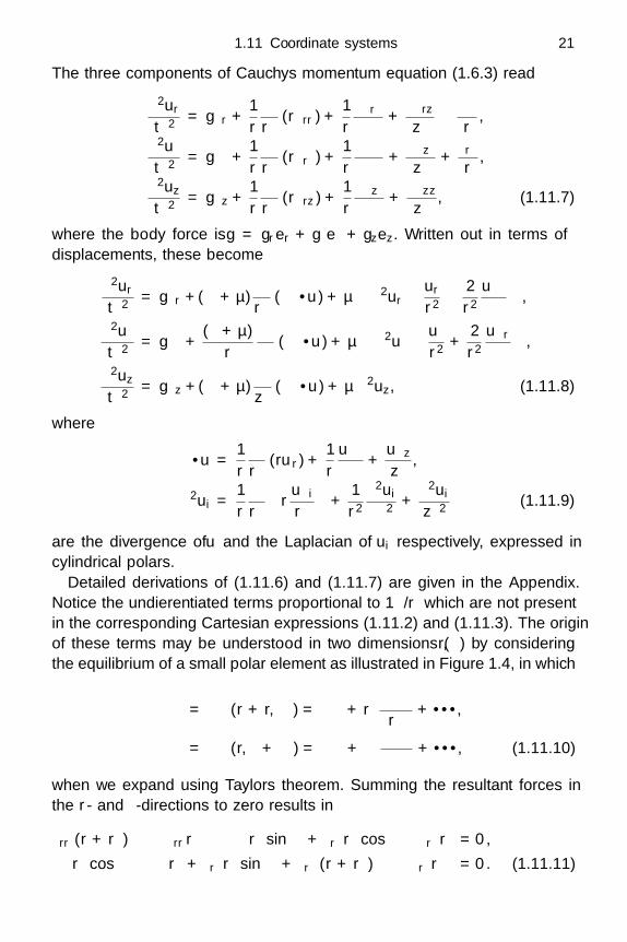
Detailed derivations of (1.11.6) and (1.11.7) are given in the Appendix.Notice the undifferentiated terms proportional to 1/r which are not presentin the corresponding Cartesian expressions (1.11.2) and (1.11.3). The originof these terms may be understood in two dimensions (r, θ) by consideringthe equilibrium of a small polar element as illustrated in Figure 1.4, in which
ταβ = ταβ(r + δr, θ) = ταβ + δr∂ταβ
∂r+ · · · ,
ταβ = ταβ(r, θ + δθ) = ταβ + δθ∂ταβ
∂θ+ · · · , (1.11.10)
when we expand using Taylor’s theorem. Summing the resultant forces inthe r- and θ-directions to zero results in
τrr (r + δr) δθ − τrrrδθ − τθθδr sin δθ + τrθδr cos δθ − τrθδr = 0,
τθθδr cos δθ − τθθδr + τrθδr sin δθ + τrθ (r + δr) δθ − τrθrδθ = 0. (1.11.11)
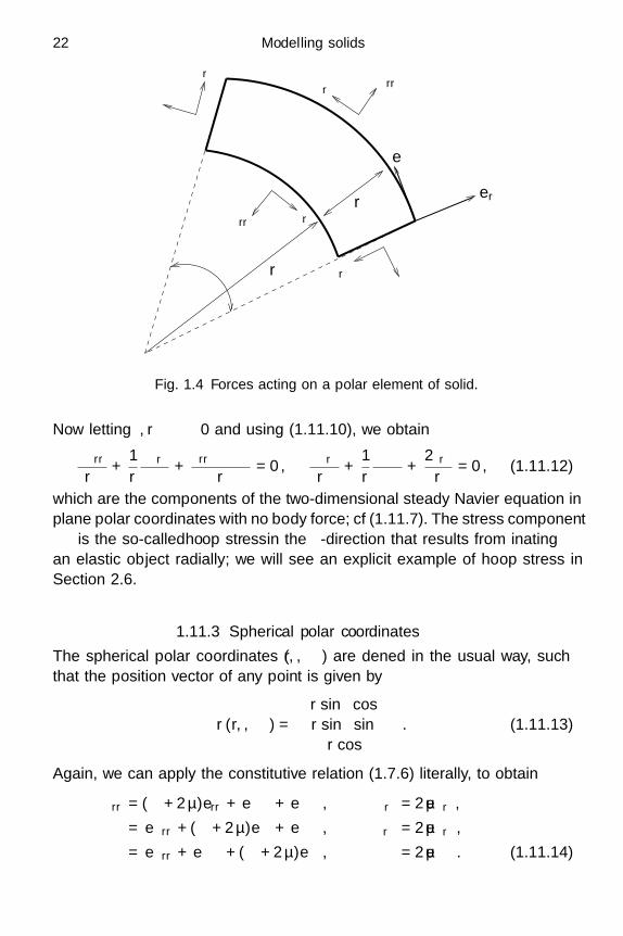
22 Modelling solids
τθθ
τrθ
δθ
τrθ τrr
eθ
τθθ
δrτrr
τrθ
r τrθ
er
Fig. 1.4 Forces acting on a polar element of solid.
Now letting δθ, δr → 0 and using (1.11.10), we obtain
∂τrr
∂r+
1r
∂τrθ
∂θ+
τrr − τθθ
r= 0,
∂τrθ
∂r+
1r
∂τθθ
∂θ+
2τrθ
r= 0, (1.11.12)
which are the components of the two-dimensional steady Navier equation inplane polar coordinates with no body force; cf (1.11.7). The stress componentτθθ is the so-called hoop stress in the θ-direction that results from inflatingan elastic object radially; we will see an explicit example of hoop stress inSection 2.6.
1.11.3 Spherical polar coordinates
The spherical polar coordinates (r, θ, φ) are defined in the usual way, suchthat the position vector of any point is given by
r(r, θ, φ) =
r sin θ cos φ
r sin θ sinφ
r cos θ
. (1.11.13)
Again, we can apply the constitutive relation (1.7.6) literally, to obtain
τrr = (λ + 2µ)err + λeθθ + λeφφ, τrθ = 2µerθ,
τθθ = λerr + (λ + 2µ)eθθ + λeφφ, τrφ = 2µerφ,
τφφ = λerr + λeθθ + (λ + 2µ)eφφ, τθφ = 2µeθφ. (1.11.14)

1.11 Coordinate systems 23
The linearised strain components are now given by
err =∂ur
∂r, 2erθ =
1r
∂ur
∂θ+
∂uθ
∂r− uθ
r,
eθθ =1r
(∂uθ
∂θ+ ur
), 2erφ =
1r sin θ
∂ur
∂φ+
∂uφ
∂r− uφ
r,
eφφ =1
r sin θ
∂uφ
∂φ+
ur
r+
uθ cot θ
r, 2eθφ =
1r sin θ
∂uθ
∂φ+
1r
∂uφ
∂θ− uφ cot θ
r.
(1.11.15)
Cauchy’s equation of motion leads to the three equations
ρ∂2ur
∂t2= ρgr +
1r2
∂(r2τrr)∂r
+1
r sin θ
∂(sin θτrθ)∂θ
+1
r sin θ
∂τrφ
∂φ− τθθ + τφφ
r,
ρ∂2uθ
∂t2= ρgθ +
1r2
∂(r2τrθ)∂r
+1
r sin θ
∂(sin θτθθ)∂θ
+1
r sin θ
∂τθφ
∂φ+
τrθ − cot θτφφ
r,
ρ∂2uφ
∂t2= ρgφ +
1r2
∂(r2τrφ)∂r
+1
r sin θ
∂(sin θτθφ)∂θ
+1
r sin θ
∂τφφ
∂φ+
τrφ + cot θτθφ
r, (1.11.16)
where the body force is g = grer+gθeθ+gφeφ. Again, (1.11.15) and (1.11.16)may be derived using the general approach given in the Appendix or moredirectly by analysing a small polar element. In terms of displacements, theNavier equation reads
ρ∂2ur
∂t2= ρgr + (λ + µ)
∂
∂r(∇ · u)
+ µ
∇2ur −
2ur
r2 − 2r2 sin θ
∂
∂θ(uθ sin θ) − 2
r2 sin θ
∂uφ
∂φ
,
ρ∂2uθ
∂t2= ρgθ +
(λ + µ)r
∂
∂θ(∇ · u)
+ µ
∇2uθ +
2r2
∂ur
∂θ− uθ
r2 sin2 θ− 2 cos θ
r2 sin2 θ
∂uφ
∂φ
,
24 Modelling solids
ρ∂2uφ
∂t2= ρgφ +
(λ + µ)r sin θ
∂
∂φ(∇ · u)
+ µ
∇2uφ +
2r2 sin θ
∂ur
∂φ+
2 cos θ
r2 sin2 θ
∂uθ
∂φ− uφ
r2 sin2 θ
, (1.11.17)
where
∇ · u =1r2
∂
∂r
(r2ur
)+
1r sin θ
∂
∂θ(sin θuθ) +
1r sin θ
∂uφ
∂φ,
∇2ui =1r2
∂
∂r
(r2 ∂ui
∂r
)+
1r2 sin θ
∂
∂θ
(sin θ
∂ui
∂θ
)+
1r2 sin2 θ
∂2ui
∂φ2 .
(1.11.18)
Exercises
1.1 A light spring of natural length L and spring constant k hangs freelywith a mass m attached to one end and the other end fixed. Showthat the length of the spring satisfies the differential equation
md2
dt2+ k( − L) − mg = 0.
Deduce that
12m
(d
dt
)2
+12k( − L)2 + mg(L − ) = const.
and interpret this result in terms of energy.1.2 A string, stretched to a tension Talong the x-axis, undergoes small
transverse displacements such that its position at time t is givenby the graph z = w(x, t). Given that w satisfies the wave equation(1.10.9), where is the mass per unit length of the string, show that,if x = a and x = b are any two points along the string,
ddt
12
∫ b
a
(∂w
∂t
)2
dx +∫ b
a
12
(∂w
∂x
)2
T dx
=[T
∂w
∂x
∂w
∂t
]b
a
.
Interpret this result in terms of conservation of energy.1.3 A system of masses m along the x-axis at positions Xn = nL
(n = 0, 1, 2, . . .) are linked by springs satisfying Hooke’s law (1.2.1),as shown in Figure 1.5. If each mass is displaced by a distance un(t),show that the tension Tn joining Xn to Xn+1 satisfies
Tn − Tn−1 = md2un
dt2, where Tn = k (un+1 − un).

Exercises 25
m mmTn−1 Tn−1 Tn Tn
unun−1 un+1
Fig. 1.5 A system of masses connected by springs along the x-axis.
Deduce that
md2un
dt2= k (un+1 − 2un + un−1)
and show that this is a spatial discretisation of the partial differentialequation
∂2u
∂t2= c2 ∂2u
∂X2 ,
where X = nL, un(t) = u(X, t) and c2 = kL2/m.[It is not so easy to use discrete element models in more than
one dimension; for example, it can be shown that it is impossible toretrieve the Navier equation as the limit of a lattice of masses joinedby springs aligned along three orthogonal axes.]
1.4 If x, x′, u and u′ are related by (1.4.9), use the chain rule to showthat
∂u′i
∂x′j
= piαpjβ∂uα
∂xβ.
Hence establish equation (1.4.11) to show that Eij transforms as atensor under a rotation of the coordinate axes.
[Hint: note that, since P is orthogonal, pklpkm ≡ δlm.]1.5 Consider a volume V (t) that is fixed in a deforming solid body. Show
that conservation of angular momentum for V (t) leads to the equa-tion
ddt
∫∫∫V (t)
x×∂u
∂tρ dx =
∫∫∫V (t)
x×gρ dx +∫∫
∂V (t)x×(τn) da.
From this and Cauchy’s momentum equation (1.6.3), deduce thatτij ≡ τji.
1.6 Show that the linearised strain eij , given by (1.7.1), is identically zeroif and only if u = c + ω×x, where c and ω are spatially-uniformvectors. Show that this approximates the rigid-body motion (1.4.13)when P is close to I. If u is of this form, and known to be zero atthree non-collinear points, deduce that c = ω = 0.

26 Modelling solids
1.7 By writing the linearised strain tensor eij as the sum of a zero-trace contribution eij − (1/3)δijekk and a purely diagonal contribu-tion (1/3)δijekk , show that W can be rewritten as
W =(
λ
2+
µ
3
)(ekk)
2 + µ
(eij −
13δijekk
)(eij −
13δijekk
).
Deduce that, for W to have a single global minimum at eij = 0, it issufficient for µ and λ+2µ/3 to be positive. By considering particularvalues of eij , show that it is also necessary.
1.8 Suppose a solid body occupies the region D and the displacement u
is prescribed on ∂D. Let
U =∫∫∫
DW − ρg · u dx,
where W is the strain energy density. Show that, if ui is changed bya small virtual displacement ηi, then the corresponding leading-orderchange in U is
δU =∫∫∫
D
(∂ηi
∂xjτij − ρgiηi
)dx.
[Hint: use the fact that τij is symmetric.] Use the divergence theoremto show that
δU =∫∫
∂Dηiτijnj da −
∫∫∫D
(∂τij
∂xj+ ρgi
)ηi dx,
and deduce that the minimisation of U with respect to all displace-ments satisfying the given boundary condition leads to the steadyNavier equation. Deduce also that, if no boundary condition is im-posed, the natural boundary condition is the vanishing of the tractionτijnj on ∂D.
Show also that the minimisation of U subject to the constraintdiv u ≡ 0 leads to the steady incompressible Navier equation (1.8.3a),where p is a Lagrange multiplier.
1.9 An elastic body D at rest is subject to a traction τn = σ(x) on itsboundary ∂D. By taking the cross product of x with (1.10.2) beforeintegrating over D, derive (1.10.7) and deduce that the net momentacting on D must be zero.
1.10 Suppose that u satisfies the steady Navier equation (1.10.2) in aregion D and the mixed boundary condition α(x)u+β(x)τn = f(x)on ∂D. Show that, if a solution exists, it is unique provided α > 0and β 0.

Exercises 27
[If α and β take different signs, then there is no guarantee ofuniqueness. This is analogous to the difficulty associated with theRobin boundary condition for scalar elliptic partial differential equa-tions (Ockendon et al., 2003, p. 154).]
1.11 (a) Show that, in plane polar coordinates (r, θ), the basis vectorssatisfy
der
dθ= eθ,
deθ
dθ= −er.
(b) Consider a small line segment joining two particles whose po-lar coordinates are (r, θ) and (r + δr, θ + δθ). Show that thevector joining the two particles is given to leading order by
δX ∼ δrer + rδθeθ.
(c) If a two-dimensional displacement field is imposed, withu = ur(r, θ)er(θ) + uθ(r, θ)eθ(θ), show that the line elementδX is displaced to
δx = δX +(
∂ur
∂rδr +
∂ur
∂θδθ − uθδθ
)er
+(
∂uθ
∂rδr +
∂uθ
∂θδθ + urδθ
)eθ.
(d) Hence show that
|δx|2 = |δX|2 +(δr, rδθ)
(err erθ
erθ eθθ
)(δr
rδθ
)where, to leading order in the displacements,
err =∂ur
∂r, 2erθ =
1r
∂ur
∂θ+
∂uθ
∂r− uθ
r, eθθ =
1r
(∂uθ
∂θ+ ur
).
[These are the elements of the linearised strain tensor in planepolar coordinates, as in (1.11.6).]

2
Linear elastostatics
2.1 Introduction
This chapter concerns steady state problems in linear elasticity. This topicmay appear to be the simplest in the whole of solid mechanics, but we willfind that it offers many interesting mathematical challenges. Moreover, thematerial presented in this chapter will provide crucial underpinning to themore general theories of later chapters.
We will begin by listing some very simple explicit solutions which givevaluable intuition concerning the role of the elastic moduli introduced inChapter 1. Our first application of practical importance is elastic torsion,which concerns the twisting of an elastic bar. This leads to a class of exactsolutions of the Navier equation in terms of solutions of Laplace’s equationin two dimensions. However, as distinct from the use of Laplace’s equationin, say, hydrodynamics or electromagnetism, the dependent variable is thedisplacement, which has a direct physical interpretation, rather than a po-tential, which does not. This means we have to be especially careful to ensurethat the solution is single-valued in situations involving multiply-connectedbars.
These remarks remain important when we move on to another class oftwo-dimensional problems called plane strain problems. These have evenmore general practical relevance but involve the biharmonic equation. Thisequation, which will be seen to be ubiquitous in linear elastostatics, posessignificant extra difficulties as compared to Laplace’s equation. In particular,we will find that it is much more difficult to construct explicit solutions using,for example, the method of separation of variables.
An interesting technique to emerge from both these classes of problems isthe use of stress potentials, which are the elastic analogues of electrostatic orgravitational potentials, say, or the stream function in hydrodynamics. We
28

2.2 Linear displacements 29
will find that a large class of elastostatic problems with some symmetry, forexample two-dimensional or axisymmetric, can be described using a singlescalar potential that satisfies the biharmonic equation.
Fully three-dimensional problems are mostly too difficult to be suitable forthis chapter. Nonetheless, we will be able to provide a conceptual frameworkwithin which to represent the solution by generalising the idea of Green’sfunctions for scalar ordinary and partial differential equations. The necessaryGreen’s tensor describes the response of an elastic body to a localised pointforce applied at some arbitrary position in the body. This idea opens up oneof the most distinctive and fascinating aspects of linear elasticity: becauseof the intricacy of (1.7.8), many different kinds of singular solutions canbe constructed using stress functions and Green’s tensors, each being theresponse to a different kind of localised forcing, and the catalogue of thesedifferent responses is a very helpful toolkit for thinking about solid mechanicsmore generally.
2.2 Linear displacements
We will begin by neglecting the body force g so the steady Navier equationreduces to
∇ · τ = (λ + µ) grad div u + µ∇2u = 0. (2.2.1)
This vector partial differential equation for u is the starting point for allwe will say in this chapter. As discussed in Section 1.10, it needs to besupplemented with suitable boundary conditions, which will vary dependingon the situation being modelled.
If the displacement u is a linear function of position x, then the straintensor E is spatially uniform. It follows that the stress tensor τ is also uniformand, therefore, trivially satisfies (2.2.1). Such solutions provide considerableinsight into the predictions of (2.2.1) and also give a feel for the significanceof the parameters λ and µ. To avoid suffices, we will write u = (u, v, w)T
and x = (x, y, z)T.
2.2.1 Isotropic expansion
As a first example, suppose
u =α
3x, (2.2.2)
where α is a constant scalar, which must be small for linear elasticity to bevalid. When α > 0, this corresponds to a uniform isotropic expansion of the

30 Linear elastostatics
(a)(c)(b)
1 + α/3
1 + α/3
1 + α/3
1
11y
x
z
α 1 − αν
1 − αν
1 + α
Fig. 2.1 A unit cube undergoing (a) uniform expansion (2.2.2), (b) one-dimensionalshear (2.2.6), (c) uniaxial stretching (2.2.8).
medium so that, as illustrated in Figure 2.1(a), a unit cube is transformedto a cube with sides of length 1 + α/3. (Of course, if α is negative, thedisplacement is an isotropic contraction.) Since α is small, the relative changein volume is thus (
1 +α
3
)3− 1 ∼ α. (2.2.3)
The strain and stress tensors corresponding to this displacement field aregiven by
eij =α
3δij and τij =
(λ +
23µ
)αδij . (2.2.4)
This is a so-called hydrostatic situation, in which the stress is characterisedby a scalar isotropic pressure p, and τij = −pδij . The pressure is related tothe relative volume change by p = −Kα, where
K = λ +23µ (2.2.5)
measures the resistance to expansion or compression and is called the bulkmodulus or modulus of compression; from Exercise 1.7, we know that K ispositive.
2.2 Linear displacements 31
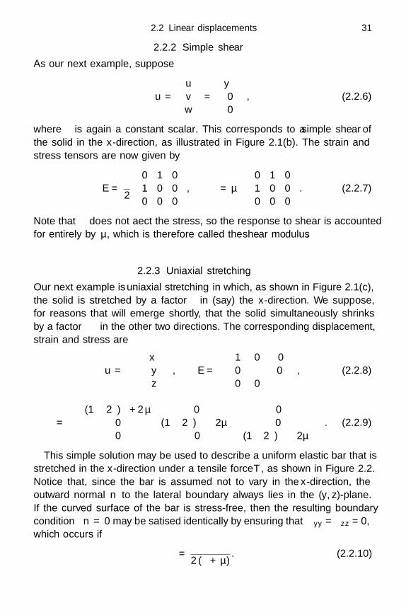
2.2.2 Simple shear
As our next example, suppose
u =
u
v
w
=
αy
00
, (2.2.6)
where α is again a constant scalar. This corresponds to a simple shear ofthe solid in the x-direction, as illustrated in Figure 2.1(b). The strain andstress tensors are now given by
E =α
2
0 1 01 0 00 0 0
, τ = αµ
0 1 01 0 00 0 0
. (2.2.7)
Note that λ does not affect the stress, so the response to shear is accountedfor entirely by µ, which is therefore called the shear modulus.
2.2.3 Uniaxial stretching
Our next example is uniaxial stretching in which, as shown in Figure 2.1(c),the solid is stretched by a factor α in (say) the x-direction. We suppose,for reasons that will emerge shortly, that the solid simultaneously shrinksby a factor να in the other two directions. The corresponding displacement,strain and stress are
u = α
x
−νy
−νz
, E = α
1 0 00 −ν 00 0 −ν
, (2.2.8)
τ = α
(1 − 2ν)λ + 2µ 0 00 (1 − 2ν)λ − 2νµ 00 0 (1 − 2ν)λ − 2νµ
. (2.2.9)
This simple solution may be used to describe a uniform elastic bar that isstretched in the x-direction under a tensile force T , as shown in Figure 2.2.Notice that, since the bar is assumed not to vary in the x-direction, theoutward normal n to the lateral boundary always lies in the (y, z)-plane.If the curved surface of the bar is stress-free, then the resulting boundarycondition τn = 0 may be satisfied identically by ensuring that τyy = τzz = 0,which occurs if
ν =λ
2 (λ + µ). (2.2.10)

32 Linear elastostatics
τn = 0
z
y
x AT T
Fig. 2.2 A uniform bar being stretched under a tensile force T .
Hence the bar, while stretching by a factor α in the x-direction, must shrinkby a factor να in the two transverse directions; if ν happened to be neg-ative, this would correspond to an expansion. The ratio ν between lateralcontraction and longitudinal extension is called Poisson’s ratio.
With ν given by (2.2.10), the stress tensor has just one non-zero element,namely
τxx = Eα, (2.2.11)
where
E =µ(3λ + 2µ)
λ + µ(2.2.12)
is called Young’s modulus. If the cross-section of the bar has area A, thenthe tensile force T applied to the bar is related to the stress by
T = Aτxx = AEα; (2.2.13)
thus AE is the elastic modulus k′ referred to in (1.2.2). By measuring T , thecorresponding extensional strain α and transverse contraction να, one maythus infer the values of E and ν for a particular solid from a bar-stretchingexperiment like that illustrated in Figure 2.2. The Lame constants may thenbe evaluated using
λ =νE
(1 + ν)(1 − 2ν), µ =
E
2(1 + ν). (2.2.14)
We note that the constitutive relation (1.7.7) can be written in terms of E
and ν as
Eeij = (1 + ν)τij − ντkkδij . (2.2.15)
While E is a positive constant with the dimensions of pressure, ν is dimen-sionless and constrained on physical grounds to lie in the range−1 < ν < 1/2. The lower bound for ν comes from the condition λ+2µ/3 > 0

2.2 Linear displacements 33
(a)
(b)
Fig. 2.3 A paper model with negative Poisson’s ratio. Each line segment is a stripof paper viewed end-on.
required for convexity of the strain energy, as shown in Exercise 1.7. The up-per bound ν → 1/2 is approached as λ → ∞, in other words as the materialbecomes incompressible, as discussed in Section 1.8.
For most solids, ν is positive, but it is possible (see Figure 2.3) to constructsimple hinged paper models with negative Poisson’s ratio; try extending acrumpled piece of paper! So-called auxetic materials, in which ν < 0, havebeen developed whose microscopic structure mimics such paper models sothey also display negative values of ν and they expand in all directions whenpulled in only one (see Lakes, 1987).
2.2.4 Biaxial strain
As a final illustrative example, we generalise Section 2.2.3 and consider anelastic plate strained in the (x, y)-plane as illustrated in Figure 2.4. Supposethe plate experiences a linear in-plane distortion while shrinking by a factorγ in the z-direction, so the displacement is given by
u =
u
v
w
=
ax + by
cx + dy
−γz
, (2.2.16)
and, as in Section 2.2.3, the stress and strain tensors are both constant. Herewe choose γ to satisfy the condition τzz = 0 on the traction-free upper and
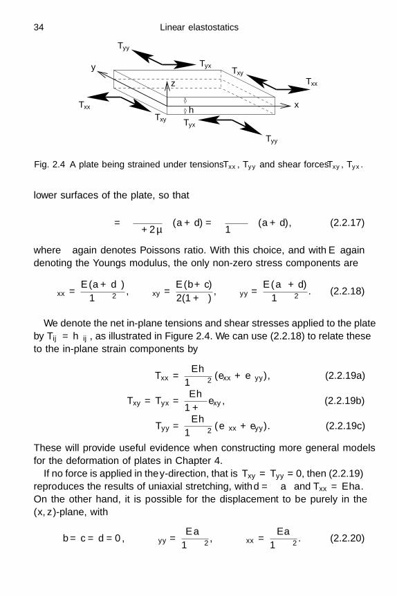
34 Linear elastostatics
y
x
z
h
Tyx
Txx
Txx
Tyy
Txy
Tyx
Tyy
Txy
Fig. 2.4 A plate being strained under tensions Txx , Tyy and shear forces Txy , Tyx .
lower surfaces of the plate, so that
γ =(
λ
λ + 2µ
)(a + d) =
(ν
1 − ν
)(a + d), (2.2.17)
where ν again denotes Poisson’s ratio. With this choice, and with E againdenoting the Young’s modulus, the only non-zero stress components are
τxx =E(a + νd)
1 − ν2 , τxy =E(b + c)2(1 + ν)
, τyy =E(νa + d)
1 − ν2 . (2.2.18)
We denote the net in-plane tensions and shear stresses applied to the plateby Tij = hτij , as illustrated in Figure 2.4. We can use (2.2.18) to relate theseto the in-plane strain components by
Txx =Eh
1 − ν2 (exx + νeyy), (2.2.19a)
Txy = Tyx =Eh
1 + νexy, (2.2.19b)
Tyy =Eh
1 − ν2 (νexx + eyy). (2.2.19c)
These will provide useful evidence when constructing more general modelsfor the deformation of plates in Chapter 4.
If no force is applied in the y-direction, that is Txy = Tyy = 0, then (2.2.19)reproduces the results of uniaxial stretching, with d = −νa and Txx = Eha.On the other hand, it is possible for the displacement to be purely in the(x, z)-plane, with
b = c = d = 0, τyy =Eνa
1 − ν2 , τxx =Ea
1 − ν2 . (2.2.20)

2.2 Linear displacements 35
Thus a transverse stress τyy must be applied to prevent the plate fromcontracting in the y-direction when we stretch it in the x-direction. Noticealso that the effective elastic modulus E/(1− ν2) is larger than E wheneverν is non-zero, which shows that purely two-dimensional stretching is alwaysmore strenuous than uniaxial stretching.
2.2.5 General linear displacements
The simple linear examples considered above shed useful light on more gen-eral solutions of the Navier equation. Indeed, any displacement field, whenexpanded in a Taylor series about some point x0, is linear to leading order:
u(x) = u(x0) +(∇u (x0)
)T(x − x0) + · · · . (2.2.21)
Here ∇u is the displacement gradient matrix, whose entries are conven-tionally defined to be ∇u = (∂uj/∂xi), and may be written as the sum ofsymmetric and skew-symmetric parts:
∂uj
∂xi=
12
(∂ui
∂xj+
∂uj
∂xi
)+
12
(∂uj
∂xi− ∂ui
∂xj
). (2.2.22)
We recognise the symmetric part of ∇u as the linear strain tensor E , whilethe skew-symmetric part may be written in the form
12(∇u − ∇uT) =
0 −ω3 ω2
ω3 0 −ω1
−ω2 ω1 0
, (2.2.23)
so that, with ω = (ω1, ω2, ω3)T, (2.2.21) becomes
u(x) = u0 + ω×(x − x0) + E(x − x0) + · · · . (2.2.24)
The terms on the right-hand side represent a small rigid-body translationand rotation, followed by a linear deformation characterised by the matrix E .
Since E is real and symmetric, it has real eigenvalues, say ε1, ε2, ε3, andorthogonal eigenvectors. These eigenvalues are referred to as the principalstrains, and the directions defined by the eigenvectors as the principal di-rections. If we use an orthogonal matrix P to align the coordinate axes withthese principal directions, that is
x = x0 + PTx′, (2.2.25)
then E , u, ω are transformed to E ′, u′, ω′ such that
u′ = u′0 + ω′×x′ + E ′x′ + · · · , (2.2.26)

36 Linear elastostatics
where
E ′ = PEPT =
ε1 0 00 ε2 00 0 ε3
. (2.2.27)
We can hence think of the strain at any point as comprising three orthogo-nal expansions or contractions, depending on the signs of ε1, ε2, ε3, followedby a small rigid-body rotation. Generalising Section 2.2.1, we note that thenet relative volume change associated with this expansion/contraction is
(1 + ε1)(1 + ε2)(1 + ε3) − 1 = ε1 + ε2 + ε3 + · · · . (2.2.28)
The sum of the eigenvalues is the invariant trace of the matrix E so that therelative volume change is
Tr (E) = ekk = ∇ · u. (2.2.29)
With respect to the principal axes, the stress tensor is also diagonal, namely
τ ′ =
τ1 0 00 τ2 00 0 τ3
, where
τ1 = λ(ε1 + ε2 + ε3) + 2µε1,
τ2 = λ(ε1 + ε2 + ε3) + 2µε2,
τ3 = λ(ε1 + ε2 + ε3) + 2µε3, (2.2.30)
and the eigenvalues τ1, τ2, τ3 are called the principal stresses.As an illustration, let us re-examine the simple shear of Section 2.2.2. The
eigenvalues and corresponding eigenvectors vi of E are readily found to be
ε1 =α
2, ε2 = −α
2, ε3 = 0, (2.2.31a)
v1 =
110
, v2 =
1−10
, v3 =
001
. (2.2.31b)
Hence the shear is equivalent to an expansion of magnitude α/2 in the di-rection (1, 1, 0)T plus an equal and opposite contraction in the direction(1,−1, 0)T. In the original non-principal axes, we can decompose the dis-placement as follows:
u =
αy
00
=α
2
y
−x
0
+α
4
x + y
x + y
0
− α
4
x − y
y − x
0
. (2.2.32)
The terms on the right-hand side represent a rigid-body rotation, an expan-sion and an orthogonal contraction.

2.3 Antiplane strain 37
In general, the strain tensor E and, therefore, the principal strains εi andprincipal stresses τi are functions of position x. At any such position, thestrain and stress tensors are diagonal only with respect to the principal axes;if these axes are rotated by another orthogonal matrix Q, then the strainand stress tensors become E ′′ and τ ′′ respectively, where
E ′′ = QE ′QT, τ ′′ = Qτ ′QT. (2.2.33)
It is easiest to understand the consequence of such a rotation in two dimen-sions, when we can take
Q =(
cos θ sin θ
−sin θ cos θ
)(2.2.34)
and (2.2.33b) becomes
τ ′′ =(
τ1 cos2 θ + τ2 sin2 θ (τ1 − τ2) sin θ cos θ
(τ1 − τ2) sin θ cos θ τ2 cos2 θ + τ1 sin2 θ
), (2.2.35)
with an analogous expression for E . It follows that the diagonal elements ofthe stress tensor, known as the normal stresses, always lie between min(τi)and max(τi). However, the off-diagonal shear stress takes its maximum value|τ1 − τ2|/2 when θ = ±π/4.
It is shown in Exercise 2.9 that these properties also hold for three-dimensional stress fields. In particular, the maximum shear stress alwaysoccurs at an angle of π/4 with two of the principal axes and is given by
S = maxi,j
|τi − τj |2
. (2.2.36)
This is often used as a diagnostic to test for failure, since many elasticmaterials, particularly metals, are susceptible to plastic deformation whensubject to excessive shear stress. The so-called Tresca criterion proposesthat a material will yield and become plastic when S exceeds some criticalyield stress τY. We will show below in Section 2.6.5 how this criterion canbe applied to predict the failure of a gun barrel, and a fuller account ofplasticity will be given in Chapter 8.
2.3 Antiplane strain
The simplest two-dimensional model for elastostatics occurs when the dis-placement u is unidirectional, u = (0, 0, w)T say, and w depends only onthe transverse coordinates (x, y). One way to create this state of antiplanestrain is to apply a tangential traction σ(x, y), in the axial direction only,

38 Linear elastostatics
surfacetraction σ
y
x
z
D
Fig. 2.5 A bar in a state of antiplane strain.
to the curved boundary of a cylindrical bar, as illustrated in Figure 2.5. Ofcourse, σ(x) must exert no net force or moment on the bar, as pointed outin Section 1.10. With the z-axis parallel to the bar, the stress tensor is
τ =
0 0 µ
∂w
∂x
0 0 µ∂w
∂y
µ∂w
∂xµ
∂w
∂y0
. (2.3.1)
At any point of the bar, the traction on an element normal to (cos θ, sin θ, 0)T
is µ (cos θ∂w/∂x + sin θ∂w/∂y), whose maximum value as θ varies is µ|∇w|.If we neglect gravity, the Navier equation reduces to the two-dimensionalLaplace’s equation
∂2w
∂x2 +∂2w
∂y2 = ∇2w = 0, (2.3.2)
to be solved inside the cross-section D of the bar, which is a region of the(x, y)-plane.
Since the bar is uniform, the unit normal n to the curved boundary liesin the (x, y)-plane, so the applied traction is simply a shear force σ in thez-direction that is related to w by
σ(x) = τzn = µ∂w
∂non ∂D. (2.3.3)

2.4 Torsion 39
y
z
x
M
M
D
Fig. 2.6 A bar being twisted under a moment M .
The solvability condition for the Neumann problem (2.3.2), (2.3.3) is∮∂D
σ ds = 0, (2.3.4)
which confirms that no net traction may be applied to any cross-section(cf equation (1.10.6)). If, instead of the traction, we were to specify thedisplacement w on ∂D, we would obtain the Dirichlet boundary condition
w = f(x, y) on ∂D (2.3.5)
instead of (2.3.3). We note that the strain energy density is W = µ|∇w|2and that, when the total elastic energy in the bar is minimised using thecalculus of variations, (2.3.3) with σ = 0 is the natural boundary condition(as in Exercise 1.8).
Despite its simplicity, we will find this model a very useful paradigm whenwe come to consider fracture in Chapter 7. We note that (2.3.2) also describesthe small transverse displacement w(x, y) of a nearly planar membrane undertension (Exercise 2.2); (2.3.3) and (2.3.5) then correspond to prescribingeither force or displacement at its boundary.
2.4 Torsion
Now consider a bar which, instead of stretching or contracting along its axis,twists under the action of moments applied at its ends. Such torsion barsare often used in car suspensions, and may be described by a displacementfield of the form
u =
u
v
w
=
−Ωyz
Ωxz
Ωψ(x, y)
, (2.4.1)
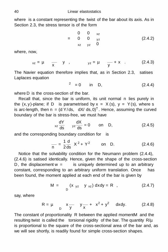
40 Linear elastostatics
where Ω is a constant representing the twist of the bar about its axis. As inSection 2.3, the stress tensor is of the form
τ =
0 0 τxz
0 0 τyz
τxz τyz 0
(2.4.2)
where, now,
τxz = µΩ(
∂ψ
∂x− y
), τyz = µΩ
(∂ψ
∂y+ x
). (2.4.3)
The Navier equation therefore implies that, as in Section 2.3, ψ satisfiesLaplace’s equation
∇2ψ = 0 in D, (2.4.4)
where D is the cross-section of the bar.Recall that, since the bar is uniform, its unit normal n lies purely in
the (x, y)-plane; if ∂D is parametrised by x = X(s), y = Y (s), where s
is arc-length, then n = (dY/ds,−dX/ds, 0)T. Hence, assuming the curvedboundary of the bar is stress-free, we must have
τxzdY
ds− τyz
dX
ds= 0 on ∂D, (2.4.5)
and the corresponding boundary condition for ψ is
∂ψ
∂n=
12
dds
(X2 + Y 2) on ∂D. (2.4.6)
Notice that the solvability condition for the Neumann problem (2.4.4),(2.4.6) is satisfied identically. Hence, given the shape of the cross-sectionD, the displacement w = Ωψ is uniquely determined up to an arbitraryconstant, corresponding to an arbitrary uniform translation. Once ψ hasbeen found, the moment applied at each end of the bar is given by
M =∫∫
D(xτyz − yτxz) dxdy = RΩ, (2.4.7)
say, where
R = µ
∫∫D
x
∂ψ
∂y− y
∂ψ
∂x+(x2 + y2) dxdy. (2.4.8)
The constant of proportionality R between the applied moment M and theresulting twist Ω is called the torsional rigidity of the bar. The quantity R/µ
is proportional to the square of the cross-sectional area of the bar and, aswe will see shortly, is readily found for simple cross-section shapes.

2.4 Torsion 41
The boundary-value problem (2.4.4), (2.4.6) for ψ may be usefully refor-mulated as follows. Whenever the stress tensor is of the form (2.4.2) andthere is no body force, the steady Navier equation reduces to
∂τxz
∂x+
∂τyz
∂y= 0. (2.4.9)
We can guarantee that (2.4.9) is satisfied by postulating the existence of astress function φ (x, y) such that
τxz = µΩ∂φ
∂y, τyz = −µΩ
∂φ
∂x, (2.4.10)
where the factors of µΩ are introduced for later convenience. Moreover, itcan be shown that the existence of φ is necessary as well as sufficient forsolutions of (2.4.9) to exist. In the same way, the existence of a streamfunction in fluid dynamics guarantees mass conservation, and the existenceof a magnetic vector potential ensures that the magnetic field is divergence-free in magnetostatics. Such potentials are never uniquely defined; in ourcase, φ is unique only up to the addition of an arbitrary constant.
By comparing (2.4.10) with (2.4.3), we see that φ and ψ are related by
∂ψ
∂x=
∂φ
∂y+ y,
∂ψ
∂y= −∂φ
∂x− x. (2.4.11)
Elimination of φ retrieves (2.4.4), while elimination of ψ reveals that φ sat-isfies Poisson’s equation
∇2φ = −2 in D. (2.4.12)
Indeed, it is easy to see from (2.4.11) that ψ and φ+(x2+y2)/2 are harmonicconjugates.
The zero-stress boundary condition (2.4.5) implies that φ is constant on∂D and, without loss of generality, we may take
φ = 0 on ∂D. (2.4.13)
The advantage of introducing the stress function φ is that the Neumannproblem for ψ has been converted to the Dirichlet problem (2.4.12), (2.4.13),which has a unique solution; exactly the same procedure could have beenapplied to the antiplane strain problem (2.3.2), (2.3.3). The torque M isthen given in terms of φ by
M = µΩ∫∫
D
(−x
∂φ
∂x− y
∂φ
∂y
)dxdy = 2µΩ
∫∫D
φ dxdy, (2.4.14)

42 Linear elastostatics
the final step being a consequence of Green’s theorem and (2.4.13). Analternative formula to (2.4.8) for the torsional rigidity is, therefore,
R = 2µ
∫∫D
φ dxdy. (2.4.15)
To illustrate the theory of this section we will now find the torsionalrigidity of a circular bar firstly using ψ and secondly using φ. If D is thedisc r < a, where (r, θ) are the usual plane polar coordinates, then theNeumann problem (2.4.4), (2.4.6) becomes
∇2ψ = 0, r < a, (2.4.16a)∂ψ
∂r= 0, r = a. (2.4.16b)
It follows that ψ is a constant and, hence, that the torsional rigidity is
R = µ
∫∫D
(x2 + y2) dxdy = µ
∫ 2π
0
∫ a
0r3 drdθ =
πµa4
2. (2.4.17)
Note that a circular cylinder is the only case in which the right-hand side of(2.4.6) is zero. For any other cross-sectional shape, twisting a bar inevitablyresults in a non-zero axial displacement w = Ωψ.
Alternatively, we may solve the Dirichlet problem (2.4.12), (2.4.13) for φ.Assuming that φ is a function only of r, we have
∇2φ =1r
ddr
(rdφ
dr
)= −2, r < a, (2.4.18a)
φ = 0, r = a, (2.4.18b)
whose solution, bounded as r → 0, is
φ =a2 − r2
2. (2.4.19)
The torsional rigidity is then given by (2.4.15):
R = µ
∫ 2π
0
∫ a
0(a2 − r2)r drdθ =
πµa4
2, (2.4.20)
which reproduces (2.4.17) as expected. This result can easily be generalisedto bars of elliptical cross section (see Exercise 2.4).
2.5 Multiply-connected domains
In Section 2.4, we have implicitly assumed that D is simply connected. Manytorsion bars are tubular in practice, and the resulting change in topology

2.5 Multiply-connected domains 43
y
x
D
z
∂Do
∂Di
Fig. 2.7 A uniform tubular torsion bar, with inner and outer free surfaces given by∂Di and ∂Do respectively.
makes a big difference to the integration of our mathematical model. We nowhave to apply the condition (2.4.5) on two stress-free boundaries, namely theinner (∂Di) and outer (∂Do) surfaces of the tube, as illustrated in Figure 2.7.As before, we can deduce that φ must be constant on each of these bound-aries, but these two constants are not necessarily equal. Hence, we may onlychoose φ to satisfy
φ = 0 on ∂Do, φ = k on ∂Di, (2.5.1)
where k is a constant. Note that k is not simply additive to φ and hencemay not be set to zero without loss of generality.
The torsional rigidity is now given by
R = −µ
∫∫D
(x
∂φ
∂x+ y
∂φ
∂y
)dxdy
= −µ
∫∫D
(∂
∂x(xφ) +
∂
∂y(yφ) − 2φ
)dxdy
= 2µ
∫∫D
φ dxdy + 2µkAi, (2.5.2)
after using Green’s theorem, where Ai is the area of the hole inside ∂Di.To obtain φ and thus R uniquely, we still have to evaluate the unknownconstant k.
By working with the stress function φ, we have reduced the torsionalrigidity problem to a seemingly innocuous Poisson equation (2.4.12) with

44 Linear elastostatics
x
y
b ax
y
b a
(b)(a)
Fig. 2.8 The cross-section of (a) a circular cylindrical tube; (b) a cut tube.
Dirichlet boundary conditions (2.5.1) on the two boundaries of the annu-lar tube. However, we have temporarily lost sight of the displacement fieldw = Ωψ, which has yet to be determined from (2.4.11). To be physicallyacceptable, ψ must be a single-valued function of (x, y), which implies that∮
C
∂ψ
∂xdx +
∂ψ
∂ydy ≡ 0 (2.5.3)
for all simple closed paths C contained in D. In fact, it is readily shown that(2.5.3) holds for all such paths if it holds when C is the inner boundary ∂Di
(see Exercise 2.5).By substituting for ψ in favour of φ, we therefore obtain∮
∂Di
∂φ
∂xdy − ∂φ
∂ydx =
∮∂Di
∂φ
∂nds = −2Ai (2.5.4)
where, as before, Ai is the area of the void in the tube cross-section. Thisconstraint gives the extra information needed to determine the constant k
and, hence, φ and R. If there are m holes in the cross-section, with φ takingthe constant value ki (i = 1, . . . , m) on each hole, then there are m relationsof the form (2.5.4) to determine the ki.
As an illustration, suppose that D is the circular annulus a < r < b inplane polar coordinates (r, θ), as illustrated in Figure 2.8(a). Assuming thatφ is a function of r alone, it must satisfy the boundary-value problem
∇2φ =1r
ddr
(rdφ
dr
)= −2, a < r < b, (2.5.5a)
φ = k, r = a, (2.5.5b)
φ = 0, r = b, (2.5.5c)

2.5 Multiply-connected domains 45
whose solution is easily found to be
φ =b2 − r2
2+(
k − b2 − a2
2
)log (r/b)log (a/b)
. (2.5.6)
We can determine k by substituting this expression for φ into (2.5.4) to give∮∂Di
∂φ
∂nds =
∫ 2π
0
dφ
dr
∣∣∣∣r=a
a dθ = −2πa2 +2π
log (a/b)
(k − b2 − a2
2
),
(2.5.7)while Ai = πa2, so (2.5.4) tells us that
k =b2 − a2
2. (2.5.8)
This value of k eliminates the logarithmic term from (2.5.6), and we mighthave anticipated that this would be necessary by recalling that ψ and φ+r2/2are harmonic conjugates. Since
φ +r2
2= const. +
(k − b2 − a2
2
)log r (2.5.9)
and −log r is the harmonic conjugate of θ, we deduce that
ψ = const. −(
k − b2 − a2
2
)θ, (2.5.10)
which is evidently a single-valued function only if k satisfies (2.5.8).We therefore find that
φ =b2 − r2
2, (2.5.11)
and it is straightforward to substitute this into (2.5.2) and obtain the tor-sional rigidity
R =µπ
2(b4 − a4) . (2.5.12)
Had we chosen to use ψ instead of φ, we would have discovered that ψ isconstant and then quickly reproduced (2.5.12) using (2.4.8). Even in thissimple radially symmetric geometry, the bother of finding the arbitrary con-stant k has outweighed the convenience of introducing a stress function.When considering multiply-connected domains it is therefore often a betteridea to return to the physical variable ψ.

46 Linear elastostatics
Notice that (2.5.12) reproduces the result (2.4.17) for a solid circular baras a tends to zero. On the other hand, if the tube is thin, so a and b arenearly equal, then
R = 2µπa4ε(1 + O (ε)
), (2.5.13)
where ε = b/a − 1 1.We can now compare this with the torsional rigidity of a tube, such as part
of an old bicycle frame, with a thin axial cut, as illustrated in Figure 2.8(b).Here the cross-section is simply connected, so that φ must satisfy
∇2φ =1r
∂
∂r
(r∂φ
∂r
)+
1r2
∂2φ
∂θ2 = −2, a < r < b, (2.5.14a)
with
φ = 0 on r = a, b, (2.5.14b)
and
φ = 0 on θ = 0, 2π. (2.5.14c)
As shown in Exercise 2.6, this problem can be solved exactly by separatingthe variables. Alternatively, if we assume that the tube is thin, then anapproximate solution may be found by performing the rescaling
r = a (1 + εξ) , (2.5.15)
where ε is again small. To lowest order in ε, (2.5.14a,b) reduces to
∂2φ
∂ξ2 = −2ε2a2, 0 < ξ < 1, (2.5.16a)
with
φ = 0 on ξ = 0, 1, (2.5.16b)
whose solution is
φ = ε2a2ξ(1 − ξ). (2.5.17)
Notice that (2.5.17) does not satisfy the boundary conditions on θ = 0, 2π.This is because there are so-called boundary layers near the cut where theθ-derivatives must be retained in (2.5.14).
For this simply-connected cross-section, we may use (2.4.15) to determinethe torsional rigidity and thus obtain, to lowest order in ε,
R = 4πµa2ε
∫ 1
0φ dξ =
2π
3µa4ε3. (2.5.18)

2.6 Plane strain 47
Comparing (2.5.18) with (2.5.13), we see that the change in topology causedby introducing the cut has a dramatic influence on the strength of the tube,reducing its torsional rigidity by two orders of magnitude!
2.6 Plane strain
2.6.1 Definition
A more common configuration than that of antiplane strain is plane strain,in which a solid is displaced in the (x, y)-plane only, with the displacementbeing independent of z. Writing
u =
u (x, y)v (x, y)
0
, (2.6.1)
we find that the stress tensor takes the form
τ =
τxx τxy 0τxy τyy 00 0 τzz
, (2.6.2)
where
τxx = λ
(∂u
∂x+
∂v
∂y
)+ 2µ
∂u
∂x, τxy = µ
(∂u
∂y+
∂v
∂x
), (2.6.3a)
τyy = λ
(∂u
∂x+
∂v
∂y
)+ 2µ
∂v
∂y, τzz = λ
(∂u
∂x+
∂v
∂y
). (2.6.3b)
This configuration arises, for example, when a z-independent traction justin the (x, y)-plane is applied to the curved boundary of a cylindrical baraligned with the z-axis. The easily-forgotten stress component τzz representsthe normal traction that would need to be applied to the ends of such a barto prevent it expanding or contracting in the z-direction.
2.6.2 The Airy stress function
With the stress tensor given by (2.6.2), and gravity neglected, the Navierequation reduces to
∂τxx
∂x+
∂τxy
∂y= 0,
∂τxy
∂x+
∂τyy
∂y= 0, (2.6.4)
or, in terms of displacements,
(λ + µ)(
∂2u
∂x2 +∂2v
∂x∂y
)+ µ
(∂2u
∂x2 +∂2u
∂y2
)= 0, (2.6.5a)
(λ + µ)(
∂2u
∂x∂y+
∂2v
∂y2
)+ µ
(∂2v
∂x2 +∂2v
∂y2
)= 0. (2.6.5b)

48 Linear elastostatics
By cross-differentiating, it is straightforward to eliminate u and v in turnfrom (2.6.5) and thus show that each satisfies the biharmonic equation
∇4u = ∇4v = 0, (2.6.6)
where ∇4 refers here to the two-dimensional biharmonic operator:
∇4 =(
∂2
∂x2 +∂2
∂y2
)(∂2
∂x2 +∂2
∂y2
)=
∂4
∂x4 + 2∂4
∂x2∂y2 +∂4
∂y4 . (2.6.7)
In fact, we can reduce (2.6.5) to a single biharmonic equation by makinguse of another potential function as follows.
By inspection, the integrability condition for the system (2.6.4) is theexistence of an Airy stress function A such that
τxx =∂2A
∂y2 , τxy = − ∂2A
∂x∂y, τyy =
∂2A
∂x2 . (2.6.8)
In the same way that the stress function φ in (2.4.10) is only defined towithin a constant, A is only defined to within a function that is linear inx and y; in other words, any such function may be added to A withoutcontributing to the stress.
By using (2.6.3), we obtain the following expressions for the displacementgradients
2µ∂u
∂x= −ν
∂2A
∂x2 + (1 − ν)∂2A
∂y2 , (2.6.9a)
2µ∂v
∂y= (1 − ν)
∂2A
∂x2 − ν∂2A
∂y2 , (2.6.9b)
µ
(∂u
∂y+
∂v
∂x
)= − ∂2A
∂x∂y. (2.6.9c)
Now, by taking ∂2/∂x∂y of (2.6.9c) and using (2.6.9a) and (2.6.9b), we caneliminate u and v and hence find that A satisfies the biharmonic equation:
∇4A = 0. (2.6.10)
Moreover, given A, (2.6.9) forms a compatible system of three equationsthat determine u and v to within a small rigid body displacement in whichu = u0 − ωy, v = v0 + ωx, with u0, v0 and ω constant.
We now recall that the general solution of Laplace’s equation in two di-mensions may be written in the form
φ = Ref (z)
, (2.6.11)
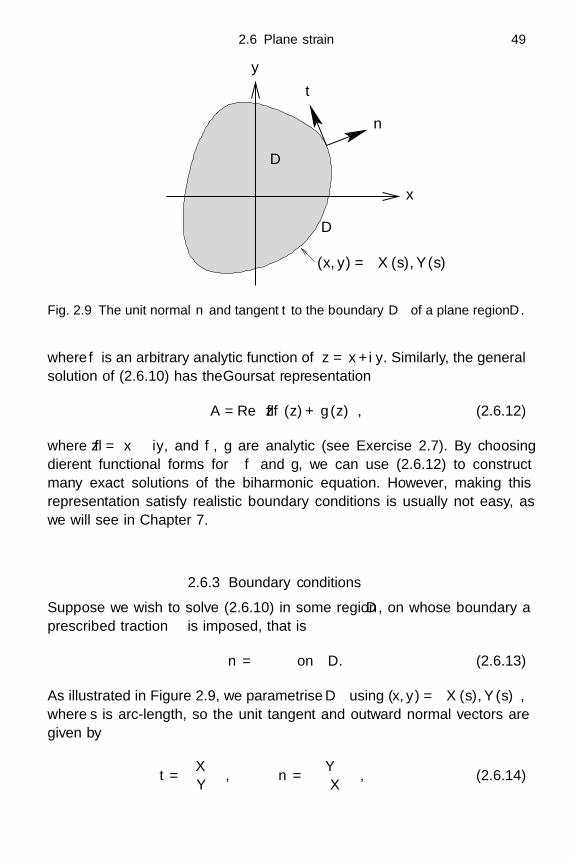
2.6 Plane strain 49
y
x
n
t
(x, y) =(X(s), Y (s)
)
D
∂D
Fig. 2.9 The unit normal n and tangent t to the boundary ∂D of a plane region D.
where f is an arbitrary analytic function of z = x+iy. Similarly, the generalsolution of (2.6.10) has the Goursat representation
A = Rezf (z) + g (z)
, (2.6.12)
where z = x − iy, and f , g are analytic (see Exercise 2.7). By choosingdifferent functional forms for f and g, we can use (2.6.12) to constructmany exact solutions of the biharmonic equation. However, making thisrepresentation satisfy realistic boundary conditions is usually not easy, aswe will see in Chapter 7.
2.6.3 Boundary conditions
Suppose we wish to solve (2.6.10) in some region D, on whose boundary aprescribed traction σ is imposed, that is
τn = σ on ∂D. (2.6.13)
As illustrated in Figure 2.9, we parametrise ∂D using (x, y) =(X(s), Y (s)
),
where s is arc-length, so the unit tangent and outward normal vectors aregiven by
t =(
X ′
Y ′
), n =
(Y ′
−X ′
), (2.6.14)
50 Linear elastostatics
where ′ is shorthand for d/ds. Using (2.6.8) to write the stress componentsin terms of A, we thus find that (2.6.13) can be written in the form
dds
(∂A/∂y
−∂A/∂x
)= σ. (2.6.15)
If no surface traction is applied, that is σ = 0, then it follows from(2.6.15) that ∇A is constant on ∂D. Since, as noted above, an arbitrarylinear function of x and y may be added to A without affecting the stresses,we can, in a simply-connected region, take this constant to be zero withoutloss of generality. Then, by taking the dot product of ∇A with t and n
respectively, we deduce that
dA
ds=
∂A
∂n= 0 (2.6.16)
on ∂D. The former of these tells us that A is constant on ∂D and, again, thisconstant may, without loss of generality, be set to zero. Finally, we arrive atthe boundary conditions
A = 0,∂A
∂n= 0 (2.6.17)
to be imposed on a stress-free boundary.We note that the divergence theorem on any closed region D yields∫
∂D
(A
∂
∂n
(∇2A
)− ∂A
∂n∇2A
)ds
=∫∫
D
div
(A grad(∇2A)
)− div
(∇2A gradA
)dxdy
=∫∫
D
A∇4A −
(∇2A
)2 dxdy. (2.6.18)
Hence, if A satisfies the biharmonic equation in D and the boundary condi-tions (2.6.17) on ∂D, then ∇2A = 0 and a second use of (2.6.17) reveals thatA ≡ 0. This result confirms that the stresses inside a closed body in planestrain are uniquely determined by the tractions applied to the boundary.
We can combine (2.6.8) and (2.6.9) to obtain the strain energy density inthe form
W =12
(τxxexx + 2τxyexy + τyyeyy)
=14µ
(1 − ν)
(∇2A
)2 + 2(
∂2A
∂x∂y
)2
− 2∂2A
∂x2∂2A
∂y2
. (2.6.19)
2.6 Plane strain 51
Then the calculus of variations can be used to show that minimisers of thenet strain energy
U =∫∫
DW dxdy
in a closed region D satisfy the biharmonic equation (2.6.10).When the displacement rather than the stress is prescribed on a boundary
in plane strain, the usefulness of the stress function A is diminished. This isbecause the displacements are related to A by (2.6.9), so boundary conditionsfor u and v cannot usually be expressed simply in terms of A. We will show inSection 2.8 that other stress functions can be defined that are better suitedto such problems.
2.6.4 Plane strain in a disc
As a first illustrative example, let us consider plane strain in a circularregion r < a on whose boundary r = a a prescribed traction is applied.We begin by deriving the relations between the Airy stress function and thestress components in polar coordinates. Recalling (1.11.7) with gi = 0 andall variables depending only on r and θ, we try writing
τθθ =∂2A
∂r2 . (2.6.20a)
Then (1.11.7b) gives −∂3A/∂r2∂θ = 2τrθ + r∂τrθ/∂r, which suggests thatwe write τrθ = ∂B/∂r. Since ∂2/∂r2(rB) is now equal to −∂3A/∂r2∂θ, wefind that
τrθ = − ∂
∂r
(1r
∂A
∂θ
), (2.6.20b)
and then (1.11.7a) gives
τrr =1r2
∂2A
∂θ2 +1r
∂A
∂r. (2.6.20c)
Equations (2.6.20) are the analogues of (2.6.8) in plane polar coordinates.The biharmonic equation for A reads
∇4A =(
∂2
∂r2 +1r
∂
∂r+
1r2
∂2
∂θ2
)2
A = 0. (2.6.21)
We will only consider here cases where a purely normal pressure P is applied,so the boundary conditions on r = a are
1r2
∂2A
∂θ2 +1r
∂A
∂r= −P,
∂
∂r
(A
r
)= 0 on r = a; (2.6.22)
52 Linear elastostatics
we obtain the latter equation by integrating the condition τrθ = 0 withrespect to θ.
The simplest case occurs if P is constant, so we expect the displacementto be purely radial and A to be a function of r alone. The problem thusreduces to (
d2
dr2 +1r
ddr
)2
A = 0, (2.6.23)
subject to the boundary conditions
A = rdA
dr= −Pa2 on r = a. (2.6.24)
It is then straightforward to solve (2.6.23) in the form
A = c1r2 + c2 + c3r2 log r + c4 log r. (2.6.25)
For the stresses to exist throughout the circle, we require A to be twicedifferentiable as r → 0 and hence, applying the boundary conditions (2.6.24),we obtain
A = −P
2(r2 + a2) . (2.6.26)
If P is not assumed to be constant, then we can solve the problem byseparating the variables in polar coordinates, using the fact that A must bea 2π-periodic function of θ. Seeking a solution of (2.6.21) in the form
A(r, θ) = f(r) sin(nθ), (2.6.27)
where n is a positive integer, we find that(d2
dr2 +1r
ddr
− n2
r2
)2
f = 0. (2.6.28)
This Euler differential equation admits the solution f(r) = rk , where k
satisfies (k2 − n2) ((k − 2)2 − n2) = 0. (2.6.29)
We must again ensure that the stress components (2.6.20) are well definedas r → 0, and now this restricts us to the solutions k = n, n + 2, that is
f(r) = c1rn+2 + c2r
n, (2.6.30)
where the ci are again arbitrary constants. For the special case n = 1, theonly physically acceptable solution is
f(r) = c1r3. (2.6.31)

2.6 Plane strain 53
P
r = ar = b
Fig. 2.10 A plane annulus being inflated by an internal pressure P .
We can take a linear combination of separable solutions that satisfy (2.6.24)and the radially-symmetric solution (2.6.26) to obtain
A = −(
r2 + a2
4
)A0
+12
∞∑n=2
(rn
(n − 1)an−2 − rn+2
(n + 1)an
)An cos(nθ) + Bn sin(nθ)
, (2.6.32)
where An and Bn are the Fourier coefficients of P , that is
An =1π
∫ 2π
0P (θ) cos(nθ) dθ, Bn =
1π
∫ 2π
0P (θ) sin(nθ) dθ. (2.6.33)
Notice that the n = 1 term does not appear in the series in (2.6.32), so it ispossible to satisfy the boundary condition (2.6.22) only if∫ 2π
0P (θ)
(cos θ
sin θ
)dθ = 0. (2.6.34)
This is simply a manifestation of the solvability condition (1.10.6) and statesthat the net force on the disc must be zero.
2.6.5 Plane strain in an annulus
Our next example concerns the inflation of a circular annulus a < r < b
under an applied internal pressure P , as illustrated in Figure 2.10. Thispractical and important instance of plane strain might model, for example,the response of a gun barrel or a diving cylinder, or even the skin of a Belgiansausage. We will only consider here a constant pressure P , the techniquesof the previous section again being appropriate when the pressure dependson θ.

54 Linear elastostatics
Assuming that A is a function of r alone, it is given by (2.6.25), but, sincewe are now solving in the annular region a < r < b, there is no a priorijustification for eliminating the logarithmic terms that cause the stress tobe ill-behaved as r → 0. We therefore have four arbitrary constants ci in(2.6.25) to be determined from the boundary conditions.
The condition of zero traction on the outer boundary r = b means, asexplained in Section 2.6.3, that we may without loss of generality set
A =dA
dr= 0 on r = b. (2.6.35a)
With A independent of θ, τrθ is identically zero, so the specified internalpressure gives us just one more boundary condition, namely
1r
dA
dr= −P on r = a. (2.6.35b)
As in Section 2.5, the vital fourth relation needed to determine the con-stants ci comes from the realisation that the annulus is multiply connected.We need A(r) to be such that the displacement ur(r) exists and is single-valued, where, from the constitutive relations (1.11.5),
1r
dA
dr= (λ + 2µ)
dur
dr+ λ
ur
r,
d2A
dr2 = λdur
dr+ (λ + 2µ)
ur
r. (2.6.36)
By cross-differentiation, we find that that the compatibility condition for ur
to exist isd3A
dr3 +1r
d2A
dr2 − 1r2
dA
dr= 0, (2.6.37)
which is satisfied by (2.6.25) only if c3 = 0. The boundary conditions (2.6.35)may then be used to evaluate the remaining three constants and hence showthat
A =Pa2
2 (b2 − a2)(r2 − a2)− Pa2b2
b2 − a2 log(r
b
). (2.6.38)
In a plane strain problem with multiple traction-free holes, we would have
A = ki,∂A
∂n= Ki (2.6.39)
on the ith hole, where the constants ki and Ki must be determined by en-suring that both displacement components (u, v) are single-valued aroundeach hole. As noted in Section 2.5, the utility of introducing a stress func-tion in such cases is negated by the difficulty of solving for all the arbi-trary constants, and it is often preferable to work with physical variables in

2.6 Plane strain 55
multiply-connected domains. By way of illustration, had we posed the an-nular problem above in terms of the radial displacement ur(r) rather thanA, we would have obtained the considerably more tractable problem
ddr
(1r
ddr
(rur))
= 0, a < r < b, (2.6.40a)
(λ + 2µ)dur
dr+ λ
ur
r= −P, r = a, (2.6.40b)
(λ + 2µ)dur
dr+ λ
ur
r= 0, r = b. (2.6.40c)
This quickly yields the solution
ur =Pa2
2 (b2 − a2)
(r
λ + µ+
b2
µr
), (2.6.41)
and we can then recover the stress components using the constitutive rela-tions (1.11.5). In our radially symmetric geometry, τrθ is zero and the onlynon zero stresses are the radial stress τrr , the hoop stress τθθ and the axialstress τzz , given respectively by
τrr =Pa2
b2 − a2
(1 − b2
r2
), τθθ =
Pa2
b2 − a2
(1 +
b2
r2
), τzz =
2νPa2
b2 − a2 ,
(2.6.42)
where ν denotes Poisson’s ratio, as usual. These results are in accordancewith (2.6.38).
We can now use the above solution to predict the failure of a gun barrelas P increases. As explained in Section 2.2.5, the Tresca criterion predictsthat the material will fail when
S = maxi,j
|τi − τj |2
= τY , (2.6.43)
where τY is the yield stress and τi are the principal stresses. Here the stresstensor is diagonal, so τi are just the three stress components given in (2.6.42).If we assume that the material has positive Poisson’s ratio† then, sinceν < 1/2 and r < b, we can deduce from (2.6.42) the inequalities
τrr < 0 < τzz < τθθ, (2.6.44)
and so the maximum shear stress is
S =τθθ − τrr
2=
Pa2b2
(b2 − a2) r2 . (2.6.45)
†for an auxetic material with ν < 0, the second inequality in (2.6.44) is reversed and the maximumshear stress may be τθ θ − τz z instead of (2.6.45)

56 Linear elastostatics
This is maximised at r = a, so we would expect a gun barrel always to yieldfirst on its inner surface, along a generator.
We can also use (2.6.45) to predict the maximum pressure P ∗ that thebarrel can withstand, namely
P ∗ = τY
(1 − a2
b2
). (2.6.46)
Notice in particular how the barrel becomes more susceptible to failure asits thickness b − a is reduced. It turns out that this is a canonical problemfor the theory of plasticity, as will be explained in Chapter 8.
2.6.6 Plane strain in a rectangle
In Section 2.6.4, we showed how plane strain in a disc can be solved by sep-arating the variables in polar coordinates. On the face of it, the procedurewas only slightly more complicated than that for solving Laplace’s equation,the extra complication arising from the application of two boundary condi-tions rather than one on r = a. In other geometries, however, solving thebiharmonic equation generally involves serious practical difficulties that arenot encountered with Laplace’s equation.
To illustrate the problems that may occur, we will now consider planestrain in a cylinder with rectangular cross-section |x| < a, |y| < b. For sim-plicity, we suppose that the faces are subject to purely tangential tractions,that is
τxx = 0, τxy = g±(y) on x = ±a, (2.6.47a)
τyy = 0, τxy = f±(x) on y = ±b, (2.6.47b)
as shown schematically in Figure 2.11. Of course the applied tractions mustexert no net force or moment, so that∫ a
−a
(f+(x) − f−(x)
)dx =
∫ b
−b
(g+(y) − g−(y)
)dy = 0, (2.6.48a)
b
∫ a
−a
(f+(x) + f−(x)
)dx − a
∫ b
−b
(g+(y) + g−(y)
)dy = 0. (2.6.48b)
The Airy stress function therefore satisfies the biharmonic equation subjectto
A = 0,∂2A
∂x∂y= −g±(y) on x = ±a, (2.6.49a)
A = 0,∂2A
∂x∂y= −f±(x) on y = ±b, (2.6.49b)
after integrating the normal stress conditions as in Section 2.6.3.

2.6 Plane strain 57
b
a
y
g−f−
g+
f+
x
Fig. 2.11 A plane rectangular region subject to tangential tractions on its faces.
The seemingly simplest solution procedure is to separate the variables,writing A(x, y) = F (x)G(y) where
F ′′′′
F+ 2
F ′′
F
G′′
G+
G′′′′
G= 0. (2.6.50)
For any fixed value of y, this is a linear, constant-coefficient, fourth-orderordinary differential equation for F (x), which suggests writing F as a com-bination of exponentials eαx. This leads to
G′′′′ + 2α2G′′ + α4G = 0 (2.6.51)
and hence to solutions of the form
A =a1y cos (αy) + a2y sin (αy) + a3 cos (αy) + a4 sin (αy)
eαx
+b1y cos (αy) + b2y sin (αy) + b3 cos (αy) + b4 sin (αy)
e−αx. (2.6.52)
Clearly a second class of separable solutions arises from exchanging theroles of x, y. All these solutions can also be derived from (2.6.12) by puttingf = Aeαz + Be−αz , g = Ceαz + De−αz .
We now need to select from (2.6.52) functions which satisfy A = 0 on|x| = a and on |y| = b. For simplicity, we suppose that the tangential trac-tions f±(x) and g±(y) are both odd functions. We can thus assume that A isan even function of x and y, which is analogous to seeking a Fourier cosineseries representation for solutions of Laplace’s equation. After a little exper-imentation, we find that α must be of the form (n+1/2)π/a or (n+1/2)π/b,for some integer n. By interchanging x and y, we can therefore construct a
58 Linear elastostatics
solution of the form
A =∑
n odd
AnFn(x) cos
(nπy
2b
)+ BnGn(y) cos
(nπx
2a
), (2.6.53)
where An and Bn are constants and the functions Fn and Gn are defined by
Fn(x) = a sinh(nπa
2b
)cosh
(nπx
2b
)− x cosh
(nπa
2b
)sinh
(nπx
2b
), (2.6.54a)
Gn(y) = b sinh(
nπb
2a
)cosh
(nπy
2a
)− y cosh
(nπb
2a
)sinh
(nπy
2a
). (2.6.54b)
In contrast to more elementary Fourier series examples, we now encountera serious difficulty when we try to determine An and Bn in terms of theapplied tractions. Considering x = a, for example, we find that
g+(y) =∑
n odd
πn
2ab
aF ′
n(a)An sin(nπy
2b
)+ b sin
(nπ
2
)BnG′
n(y)
, (2.6.55)
but sin(nπy/2b), G′n(y) do not form an orthogonal set on −b < y < b.
Hence, if we were to multiply (2.6.55) by G′m(y) and integrate over |y| < b in
the usual Fourier series procedure, we would end up with an infinite systemof equations for the constants An and Bn. We will discuss this difficultyfurther below.
2.6.7 Plane strain in a semi-infinite strip
We now present an example which is technically easier than the rectangu-lar geometry discussed above and which has wide significance in the the-ory of linear elasticity. We consider plane strain in the semi-infinite strip0 < x < ∞, −h/2 < y < h/2, with zero stress on y = ±h/2 and with pre-scribed tractions
τxx = σx(y), τxy = σy(y) (2.6.56)
on x = 0, as illustrated in Figure 2.12. Then the Airy stress function satisfiesthe biharmonic equation along with the boundary conditions
∂2A
∂y2 (0, y) = σx(y),∂2A
∂x∂y(0, y) = −σy(y), (2.6.57)
and, as in Section 2.6.3, we can choose A such that
A(x, h/2) =∂A
∂y(x, h/2) = 0. (2.6.58)
However, because the end x = 0 is not traction-free, we cannot use the sameconditions on the other face y = −h/2. All we can safely deduce from the

2.6 Plane strain 59
stress free
stress free
y
xτxx = σx(y)
τxy = σy(y)
Fig. 2.12 The tractions applied to the edge of a semi-infinite strip.
zero-stress condition is that
∂2A
∂x2 (x,−h/2) =∂2A
∂x∂y(x,−h/2) = 0, (2.6.59a)
which implies that
A(x,−h/2) = a + bx,∂A
∂y(x,−h/2) = c, (2.6.59b)
where a, b and c are constants.We can calculate these constants by insisting that A and ∇A be contin-
uous at the corners (0,±h/2); otherwise we would, in general, have pointforces or moments acting there, rather than just jump discontinuities in thetractions. By integrating (2.6.57) with respect to y, we find that
A =∫ h/2
y(η − y)σx(η) dη,
∂A
∂x=∫ h/2
yσy(η) dη,
∂A
∂y= −
∫ h/2
yσx(η) dη
(2.6.60)
on x = 0, and we deduce that
a =∫ h/2
−h/2(y + h/2) σx(y) dy, b =
∫ h/2
−h/2σy(y) dy, c = −
∫ h/2
−h/2σx(y) dy.
(2.6.61)
We would like to try to solve this problem by separating the variables, asin Section 2.6.6, but this is difficult because of the inhomogeneous boundarycondition (2.6.59b). However, we note that the function
A∞(x, y) =(h − 2y)2
8h3
4a(h + y) + 4bx(h + y) + ch(h + 2y)
(2.6.62)
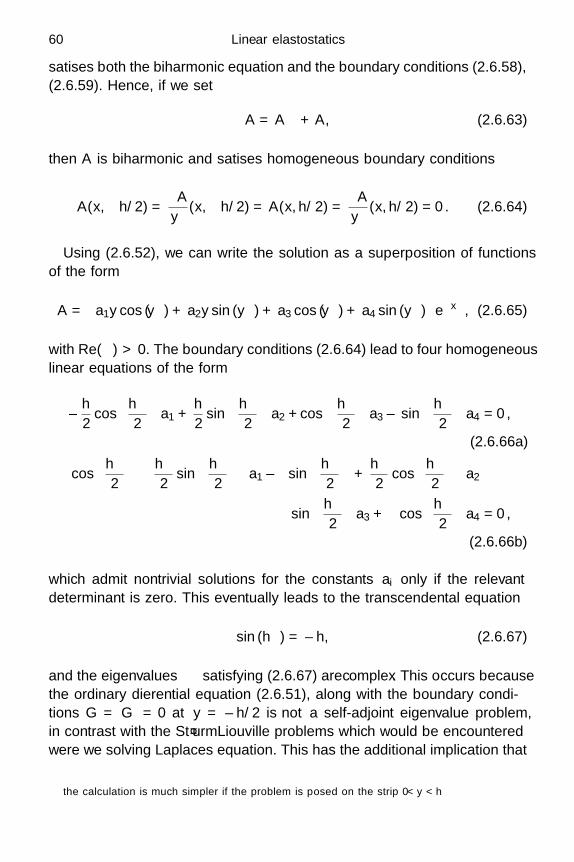
60 Linear elastostatics
satisfies both the biharmonic equation and the boundary conditions (2.6.58),(2.6.59). Hence, if we set
A = A∞ + A, (2.6.63)
then A is biharmonic and satisfies homogeneous boundary conditions
A(x,−h/2) =∂A
∂y(x,−h/2) = A(x, h/2) =
∂A
∂y(x, h/2) = 0. (2.6.64)
Using (2.6.52), we can write the solution as a superposition of functionsof the form
A =a1y cos (αy) + a2y sin (αy) + a3 cos (αy) + a4 sin (αy)
e−αx, (2.6.65)
with Re(α) > 0. The boundary conditions (2.6.64) lead to four homogeneouslinear equations of the form
±h
2cos
(αh
2
)a1 +
h
2sin
(αh
2
)a2 + cos
(αh
2
)a3 ± sin
(αh
2
)a4 = 0,
(2.6.66a)[cos
(αh
2
)− αh
2sin
(αh
2
)]a1 ±
[sin
(αh
2
)+
αh
2cos
(αh
2
)]a2
∓ α sin(
αh
2
)a3 + α cos
(αh
2
)a4 = 0,
(2.6.66b)
which admit nontrivial solutions for the constants ai only if the relevantdeterminant is zero. This eventually leads to the transcendental equation†
sin (αh) = ±αh, (2.6.67)
and the “eigenvalues” α satisfying (2.6.67) are complex. This occurs becausethe ordinary differential equation (2.6.51), along with the boundary condi-tions G = G′ = 0 at y = ±h/2 is not a self-adjoint eigenvalue problem,in contrast with the Sturm–Liouville problems which would be encounteredwere we solving Laplace’s equation. This has the additional implication that
†the calculation is much simpler if the problem is posed on the strip 0 < y < h

2.6 Plane strain 61
the “eigenfunctions” are not mutually orthogonal, which seriously compli-cates the task of fitting the initial conditions, as in (2.6.55). Had we insteadimposed the conditions A = ∂2A/∂y2 = 0 on y = ±h/2, we would havefound that the eigenvalues are real and the eigenfunctions are orthogonaltrigonometric functions. We will see a practically relevant example of thisin Section 4.6 but, unfortunately, specifying ∂2A/∂n2 on the boundary hasno obvious physical significance in plane strain.
A completeness argument can be given to show that A can in fact beexpressed as a sum of terms of the form (2.6.65), with Re(α) > 0, although,because of the difficulties described above, the coefficients can only be com-puted numerically by inverting an infinite matrix. Thus, whatever tractionsare imposed on x = 0, A will decay exponentially as x → ∞. The stress farfrom the edge of the strip will then be characterised entirely by the stressfunction A∞, which corresponds to a far-field stress, as x → ∞,
τxx → 12y(a + bx) + h(6y − h)ch3 , τxy → 3b
2h3
(h2 − 4y2) , τyy → 0.
(2.6.68)
The net tensile force T , shear force N and bending moment M exertedon any section x = const. by the stress field (2.6.68) are given by
T (x) =∫ h/2
−h/2τxx dy = −c, N(x) =
∫ h/2
−h/2τxy dy = b, (2.6.69a)
M(x) =∫ h/2
−h/2yτxx dy = a + bx +
ch
2. (2.6.69b)
From (2.6.61), we deduce that T , N and M satisfy the differential equation
dM
dx= N, (2.6.70)
and the boundary conditions
T (0) =∫ h/2
−h/2σx(y) dy, N(0) =
∫ h/2
−h/2σy(y) dy, (2.6.71a)
M(0) =∫ h/2
−h/2yσx(y) dy. (2.6.71b)
Note that (2.6.71) does not correspond to setting x = 0 as in (2.6.57); ratherit is the matching condition between (2.6.68) and the solution for A in theform (2.6.63). The only information about the tractions applied to x = 0that is preserved as x → ∞ is the value of the scalars T , N and M , which

62 Linear elastostatics
correspond to the net force and moment exerted on the edge of the strip.It follows that any system of tractions
(σx(y), σy(y)
)applied to the edge of
an elastic strip is indistinguishable from a different set of tractions whichexerts the same net force and moment, just as long as we are sufficientlyfar from the edge. This phenomenon occurs quite generally in elasticityand is known as Saint-Venant’s principle: any localised system of tractionsapplied to a sufficiently large elastic body may be characterised in the farfield purely by its net force and moment. We will return to this importantfact in Chapters 4 and 6, when considering the boundary conditions to beimposed on thin solids such as plates and rods, and we will also re-encounterthe relation (2.6.70) between the shear force and bending moment.
Finally, let us examine the far-field displacement by using (2.6.62) and(2.6.9). From (2.6.9), we find that u and v satisfy
−2µ
ν
∂v
∂y=
2µ
1 − ν
∂u
∂x=
T
h+
12M(x)yh3 , (2.6.72a)
µ
(∂u
∂y+
∂v
∂x
)=
3N
2h3
(h2 − 4y2). (2.6.72b)
We can eliminate u by differentiating (2.6.72b) with respect to x to obtain
∂2v
∂x2 = − ∂2u
∂x∂y= −
(6(1 − ν)
µh3
)M(x). (2.6.73)
This relationship between the bending moment and the curvature of thedisplaced strip will also prove very useful in Chapter 4.
2.6.8 Plane strain in a half-space
As long as we are deft with Fourier transforms, all the difficulties associatedwith the separability of solutions melt away when we consider a half-space,say y > 0, with prescribed traction
τyy = −P (x), τxy = σ(x) on y = 0. (2.6.74)
Assuming that P and σ decrease sufficiently rapidly as |x| → ∞, we definethe Fourier transform
A (k; y) =∫ ∞
−∞A (x, y) eikxdx. (2.6.75)
Assuming further that this integral converges, we also recall the inversionformula
A =12π
∫ ∞
−∞Ae−ikx dx. (2.6.76)

2.6 Plane strain 63
From the biharmonic equation (2.6.10) we find that(d2
dy2 − k2)2
A = 0 y > 0, (2.6.77a)
and, from (2.6.74),
k2A = P (k) y = 0, (2.6.77b)
ikdA
dy= σ(k) y = 0, (2.6.77c)
A → 0 y → ∞. (2.6.77d)
This ordinary differential equation for A is readily solved to give
A =(
1 + y|k|k2 P (k) − iy
kσ(k)
)e−y|k|. (2.6.78)
The presence of inverse powers of k in (2.6.78) indicates that the integralin (2.6.75) fails to converge unless k is a complex variable. However, wecan avoid the use of complex k by inverting the formulae for the stresscomponents. For simplicity, we just consider the case σ = 0, when we deducethat
τxx = −P (k) (1 − y|k|) e−|k|y , (2.6.79a)
τxy = P (k)iyke−|k|y , (2.6.79b)
τyy = −P (k) (1 + y|k|) e−|k|y , (2.6.79c)
which, as shown in Exercise 2.11(a), may be inverted as convolutions of theform
τxx = − 2π
∫ ∞
−∞P (x − s)
s2y ds
(s2 + y2)2 , (2.6.80a)
τxy = − 2π
∫ ∞
−∞P (x − s)
sy2 ds
(s2 + y2)2 , (2.6.80b)
τyy = − 2π
∫ ∞
−∞P (x − s)
y3 ds
(s2 + y2)2 . (2.6.80c)
We can now use (2.6.9) to calculate the displacements. For example, v
satisfies
2µdv
dy= −(1 − ν)k2A − ν
d2A
dy2 = ((2ν − 1) − y|k|) P (k)e−y|k|, (2.6.81)

64 Linear elastostatics
which may be integrated, in the case σ = 0, to obtain
2µv =(
y + 21 − ν
|k|
)P (k) e−y|k|. (2.6.82)
Again, this is awkward to invert as it stands (because of the |k| in thedenominator) and it is easier first to differentiate with respect to x. Asshown in Exercise 2.11(b), this leads to
µ∂v
∂x= − 1
π
∫ ∞
−∞
(1 − ν)s2 + (2 − ν)y2
(s2 + y2)2 P (x − s)sds. (2.6.83)
Alternatively, we can also obtain (2.6.83) from the identity
E∂2v
∂x2 = 2(1 + ν)∂τxy
∂x− ∂τxx
∂y+ ν
∂τyy
∂y, (2.6.84)
by using (2.6.80) and then integrating with respect to x.The displacement v0(x) = v(x, 0) of the surface caused by the imposed
pressure can now be found by carefully letting y tend to zero, as shown inExercise 2.12. When we do so, the right-hand side of (2.6.83) reduces to thesingular integral
µdv0
dx= (1 − ν)
1π−∫ ∞
−∞
P (s) ds
s − x= (1 − ν)H[P ], (2.6.85)
where H[P ] is called the Hilbert transform of P , −∫
being the principal valueintegral defined in Exercise 2.12. As shown in Exercise 2.13, this transformmay be inverted using the formula H
[H[f ]
]≡ −f , and hence we can cal-
culate the pressure required to achieve a given surface displacement v0(x),namely
P = − µ
1 − νH[v′0]. (2.6.86)
As an illustrative example, the surface displacement
v0(x) =a
1 + x2/L2 (2.6.87a)
corresponds to a surface pressure
P (x) =µa
(1 − ν)L1 − x2/L2
(1 + x2/L2)2 , (2.6.87b)
and both are plotted in Figure 2.13. Notice that in some parts a negativepressure must be applied to obtain the given bounded surface displacement.

2.6 Plane strain 65
-4 -2 2 4
0.2
0.4
0.6
0.8
1
x/L
(1 − ν)LP/µa
v0/a
Fig. 2.13 The surface displacement v0(x) of a half-space and corresponding surfacepressure P (x) defined by (2.6.87).
One can deduce generally from (2.6.85) that it is only possible to achieve alocalised displacement, with v0 → 0 as x → ±∞, if∫ ∞
−∞P (x) dx = 0, (2.6.88)
and it is therefore necessary for P to change sign. This phenomenon is anartefact of plane strain which results from the artificial constraint of zerotransverse strain, and we will see in Section 2.9.3 that it does not occur inradially symmetric problems.
The general question of the indentation produced by traction applied tothe boundary of a half-plane will be discussed further in connection with“punch” problems in Chapter 7.
2.6.9 Plane strain with a body force
The Airy stress function approach can easily be extended to plane strainunder the action of a body force that is conservative. If −g may be written asthe gradient of a potential V (x, y), then the two-dimensional Navier equationtakes the form
∂τxx
∂x+
∂τxy
∂y= ρ
∂V
∂x,
∂τxy
∂x+
∂τyy
∂y= ρ
∂V
∂y, (2.6.89)
and (2.6.8) therefore generalises to
τxx = ρV +∂2A
∂y2 , τxy = − ∂2A
∂x∂y, τyy = ρV +
∂2A
∂x2 . (2.6.90)
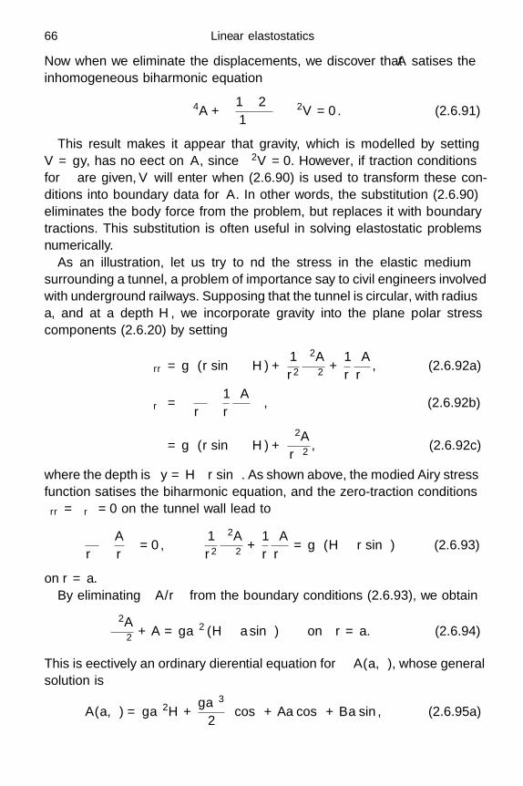
66 Linear elastostatics
Now when we eliminate the displacements, we discover that A satisfies theinhomogeneous biharmonic equation
∇4A +(
1 − 2ν
1 − ν
)∇2V = 0. (2.6.91)
This result makes it appear that gravity, which is modelled by settingV = gy, has no effect on A, since ∇2V = 0. However, if traction conditionsfor τ are given, V will enter when (2.6.90) is used to transform these con-ditions into boundary data for A. In other words, the substitution (2.6.90)eliminates the body force from the problem, but replaces it with boundarytractions. This substitution is often useful in solving elastostatic problemsnumerically.
As an illustration, let us try to find the stress in the elastic mediumsurrounding a tunnel, a problem of importance say to civil engineers involvedwith underground railways. Supposing that the tunnel is circular, with radiusa, and at a depth H, we incorporate gravity into the plane polar stresscomponents (2.6.20) by setting
τrr = ρg (r sin θ − H) +1r2
∂2A
∂θ2 +1r
∂A
∂r, (2.6.92a)
τrθ = − ∂
∂r
(1r
∂A
∂θ
), (2.6.92b)
τθθ = ρg (r sin θ − H) +∂2A
∂r2 , (2.6.92c)
where the depth is −y = H−r sin θ. As shown above, the modified Airy stressfunction satisfies the biharmonic equation, and the zero-traction conditionsτrr = τrθ = 0 on the tunnel wall lead to
∂
∂r
(A
r
)= 0,
1r2
∂2A
∂θ2 +1r
∂A
∂r= ρg (H − r sin θ) (2.6.93)
on r = a.By eliminating ∂A/∂r from the boundary conditions (2.6.93), we obtain
∂2A
∂θ2 + A = ρga2 (H − a sin θ) on r = a. (2.6.94)
This is effectively an ordinary differential equation for A(a, θ), whose generalsolution is
A(a, θ) = ρga2H +ρga3
2θ cos θ + Aa cos θ + Ba sin θ, (2.6.95a)
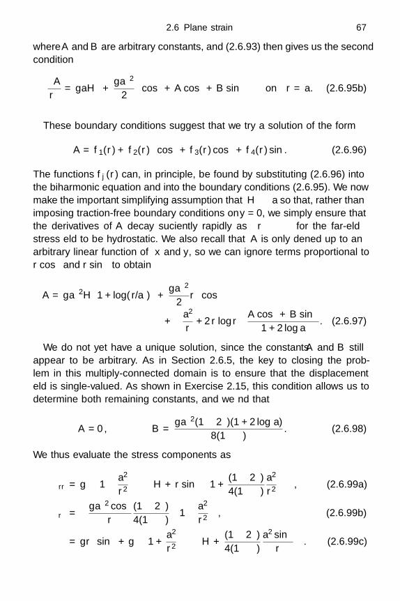
2.6 Plane strain 67
where A and B are arbitrary constants, and (2.6.93) then gives us the secondcondition
∂A
∂r= ρgaH +
ρga2
2θ cos θ + A cos θ + B sin θ on r = a. (2.6.95b)
These boundary conditions suggest that we try a solution of the form
A = f1(r) + f2(r)θ cos θ + f3(r) cos θ + f4(r) sin θ. (2.6.96)
The functions fj(r) can, in principle, be found by substituting (2.6.96) intothe biharmonic equation and into the boundary conditions (2.6.95). We nowmake the important simplifying assumption that H a so that, rather thanimposing traction-free boundary conditions on y = 0, we simply ensure thatthe derivatives of A decay sufficiently rapidly as r → ∞ for the far-fieldstress field to be hydrostatic. We also recall that A is only defined up to anarbitrary linear function of x and y, so we can ignore terms proportional tor cos θ and r sin θ to obtain
A = ρga2H(1 + log(r/a)
)+
ρga2
2rθ cos θ
+(
a2
r+ 2r log r
)A cos θ + B sin θ
1 + 2 log a. (2.6.97)
We do not yet have a unique solution, since the constants A and B stillappear to be arbitrary. As in Section 2.6.5, the key to closing the prob-lem in this multiply-connected domain is to ensure that the displacementfield is single-valued. As shown in Exercise 2.15, this condition allows us todetermine both remaining constants, and we find that
A = 0, B =ρga2(1 − 2ν)(1 + 2 log a)
8(1 − ν). (2.6.98)
We thus evaluate the stress components as
τrr = ρg
(1 − a2
r2
)−H + r sin θ
(1 +
(1 − 2ν)4(1 − ν)
a2
r2
), (2.6.99a)
τrθ = −ρga2 cos θ
r
(1 − 2ν)4(1 − ν)
(1 − a2
r2
), (2.6.99b)
τθθ = ρgr sin θ + ρg
(1 +
a2
r2
)−H +
(1 − 2ν)4(1 − ν)
a2 sin θ
r
. (2.6.99c)

68 Linear elastostatics
Evidently, τrr and τrθ are both zero on r = a, as required, and the non-zerohoop stress on the tunnel is given by
τθθ = −2ρgH +3 − 4ν
2(1 − ν)ρga sin θ on r = a. (2.6.100)
Hence a small tunnel suffers twice as much compressive stress as would occurin its absence. Moreover, the minimum compressive stress occurs at θ = π/2,which is the roof of the tunnel, while the maximum compressive stress is atthe bottom θ = −π/2. In fact, it can be shown that this final result remainsvalid for all values of H and a (see Mindlin, 1939).
2.7 Compatibility
In Section 1.6, Newton’s second law led us to write down the equation
∂τij
∂xj+ ρgi = 0 (2.7.1)
for the stress tensor in elastostatics in the presence of a body force gi.Viewed as a system of equations for the stress components, (2.7.1) is under-determined, comprising just three equations for six unknowns. It was onlyby using the constitutive relations (1.7.6),
τij = λ (ekk) δij + 2µeij = λ
(∂uk
∂xk
)δij + µ
(∂ui
∂xj+
∂uj
∂xi
)(2.7.2)
that we were able to obtain a closed system of the three Navier equationsfor the three components of displacement. It follows that, given τij , (2.7.2)is itself an over-determined system for the displacements.
If we were in the very fortunate position of knowing all the stress com-ponents τij , which of course must satisfy (2.7.1), then it would be straight-forward to obtain the corresponding linearised strain tensor from (2.2.15).Thus, given τij , we could view our expression
eij =12
(∂ui
∂xj+
∂uj
∂xi
)(2.7.3)
as a system of equations for the displacement components ui, rather than adefinition of eij . In this light, however, (2.7.3) is a set of six partial differentialequations for the three displacements ui, and this imposes on eij severerestrictions, called compatibility conditions. Since these conditions will soonbe seen to have considerable theoretical and practical importance, we willnow derive them.
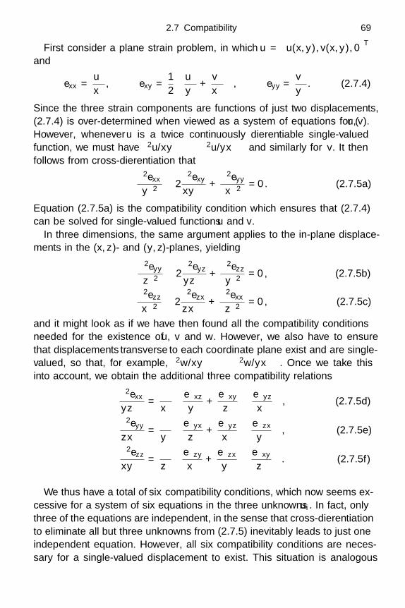
2.7 Compatibility 69
First consider a plane strain problem, in which u =(u(x, y), v(x, y), 0
)Tand
exx =∂u
∂x, exy =
12
(∂u
∂y+
∂v
∂x
), eyy =
∂v
∂y. (2.7.4)
Since the three strain components are functions of just two displacements,(2.7.4) is over-determined when viewed as a system of equations for (u, v).However, whenever u is a twice continuously differentiable single-valuedfunction, we must have ∂2u/∂x∂y ≡ ∂2u/∂y∂x and similarly for v. It thenfollows from cross-differentiation that
∂2exx
∂y2 − 2∂2exy
∂x∂y+
∂2eyy
∂x2 = 0. (2.7.5a)
Equation (2.7.5a) is the compatibility condition which ensures that (2.7.4)can be solved for single-valued functions u and v.
In three dimensions, the same argument applies to the in-plane displace-ments in the (x, z)- and (y, z)-planes, yielding
∂2eyy
∂z2 − 2∂2eyz
∂y∂z+
∂2ezz
∂y2 = 0, (2.7.5b)
∂2ezz
∂x2 − 2∂2ezx
∂z∂x+
∂2exx
∂z2 = 0, (2.7.5c)
and it might look as if we have then found all the compatibility conditionsneeded for the existence of u, v and w. However, we also have to ensurethat displacements transverse to each coordinate plane exist and are single-valued, so that, for example, ∂2w/∂x∂y ≡ ∂2w/∂y∂x. Once we take thisinto account, we obtain the additional three compatibility relations
∂2exx
∂y∂z=
∂
∂x
(∂exz
∂y+
∂exy
∂z− ∂eyz
∂x
), (2.7.5d)
∂2eyy
∂z∂x=
∂
∂y
(∂eyx
∂z+
∂eyz
∂x− ∂ezx
∂y
), (2.7.5e)
∂2ezz
∂x∂y=
∂
∂z
(∂ezy
∂x+
∂ezx
∂y− ∂exy
∂z
). (2.7.5f)
We thus have a total of six compatibility conditions, which now seems ex-cessive for a system of six equations in the three unknowns ui. In fact, onlythree of the equations are independent, in the sense that cross-differentiationto eliminate all but three unknowns from (2.7.5) inevitably leads to just oneindependent equation. However, all six compatibility conditions are neces-sary for a single-valued displacement to exist. This situation is analogous

70 Linear elastostatics
to that which arises when considering a vector field u which is the gradi-ent of a potential. In this case, it is necessary that all three components ofcurlu vanish, although only two components of curlu are independent inthe above sense. Our situation is a generalisation of this statement, since, asshown in Exercise 2.21, the compatibility conditions (2.7.5) are equivalentto the components of the tensor equation
curl (curl E)T = 0, where curl =
0 −∂/∂z ∂/∂y
∂/∂z 0 −∂/∂x
−∂/∂y ∂/∂x 0
. (2.7.6)
We also remark that any three independent compatibility equations for eij
are just as under-determined as the three equilibrium equations (2.7.1) arefor τij . Hence, the fact that the compatibility conditions ensure the exis-tence of three physically acceptable displacement components suggests that(2.7.1) will similarly guarantee the existence of three scalar stress functions.We have already encountered an application of this idea to plane strain inSection 2.6, and we will show below in Section 2.8 how it may be generalisedto non-planar problems.
It is important to note that, if eij does not satisfy (2.7.5), then there isno physically acceptable displacement field that gives rise to such a strainand it is, therefore, incompatible with linear elasticity. In Section 2.9.4 wewill discuss one physical interpretation of incompatibility in detail. Mean-while, we simply conjecture that, if we are presented with an elastic materialwhich has been deformed under the action of, say, some non-zero boundarytractions, then, when the tractions are removed, the necessary and sufficientcondition for the material to return to its pristine unstrained state is thatthe strain field in it satisfies (2.7.5), and we will see specific examples of thisin Section 8.4.
2.8 Generalised stress functions
2.8.1 General observations
By taking the divergence of the steady Navier equation (2.2.1) in the absenceof body forces, we see that div u must be a harmonic function:
∇2 (div u) = 0. (2.8.1)
If instead we take the curl of (2.2.1), we find that
curl3 u = 0. (2.8.2)

2.8 Generalised stress functions 71
and so, by taking the curl once more and using (2.8.1), we obtain
∇4u = 0. (2.8.3)
Each Cartesian component of the displacement must therefore satisfy thebiharmonic equation, as shown in Section 2.6 for plane strain. We emphasisethat (2.8.3) can only be written component-wise as
∇4u =
∇4u
∇4v
∇4w
= 0 (2.8.4)
in Cartesian coordinates; in any other coordinate systems we must use theidentity (1.7.11).
Alternatively, we may use the Helmholtz representation to write u as thesum of a gradient and a curl:
u = ∇φ + ∇×A, with ∇ · A = 0. (2.8.5)
(It may be shown that this decomposition applies to any continuously dif-ferentiable vector field u.) Substitution of (2.8.5) into (2.2.1) reveals thatthe potential functions φ and A must also satisfy the biharmonic equation
∇4φ = 0, ∇4A = 0. (2.8.6)
These results all suggest that we may be able to construct large classesof solutions of (2.2.1) by considering suitable harmonic or biharmonic scalarproblems. We have already seen some examples of this approach in planeand antiplane strain (Sections 2.3–2.6) and we will now show how analogousideas may be applied in some other commonly-occurring configurations.
2.8.2 Plane strain revisited
We begin by re-examining the theory of plane strain in the light of the con-cept of compatibility developed in Section 2.7. As we showed in Section 2.6,the two conservation laws
∂τxx
∂x+
∂τxy
∂y= 0,
∂τxy
∂x+
∂τyy
∂y= 0 (2.8.7)
imply the existence of an Airy stress function A. We then eliminated thedisplacement components to deduce that A satisfies the biharmonic equa-tion. We thus implicitly assumed compatibility of the stress tensor with aphysically acceptable displacement field.
We can make this procedure more systematic by making use of the planecompatibility condition (2.7.5a) which, when written in terms of the stress
72 Linear elastostatics
components, is
∂2τxx
∂y2 − 2∂2τxy
∂x∂y+
∂2τyy
∂x2 − ν∇2 (τxx + τyy) = 0. (2.8.8)
Now (2.8.7) and (2.8.8) form a closed system of partial differential equationsfor the stress components (τxx, τxy, τyy). If, as in Section 2.6, we write
τxx =∂2A
∂y2 , τxy = − ∂2A
∂x∂y, τyy =
∂2A
∂x2 , (2.8.9)
then the stress balance equations (2.8.7) are satisfied identically, and sub-stitution of (2.8.9) into (2.8.8) quickly retrieves the biharmonic equationfor A.
It is worth noting that an inhomogeneous equation for A of the form
∇4A = f (2.8.10)
does not, as might have been suspected from (2.6.91), correspond to theimposition of a body force. The mere existence of A implies that (2.8.7) aresatisfied, so there is no such force. Instead the right-hand side f of (2.8.10)corresponds to a distribution of incompatibility through the material, andwe will discuss in Section 2.9.4 and Chapter 8 what the physical significanceof such a configuration might be.
Now let us suppose that we do impose a body force in, say, the x-directionso that the first Navier equation (2.8.7a) is modified to
∂τxx
∂x+
∂τxy
∂y= −f. (2.8.11)
Now there is no longer an Airy stress function, but we can instead tryto obtain an integrability condition from the two remaining homogeneousequations (2.8.7b) and (2.8.8). From (2.8.7b) we deduce the existence of afunction A1(x, y) such that
τxy =∂A1
∂y, τyy = −∂A1
∂x, (2.8.12)
so the compatibility condition (2.8.8) becomes(∂2
∂y2 − ν∇2)
τxx −(
∂2
∂y2 + (1 − ν)∇2)
∂A1
∂x= 0. (2.8.13)
To write this in conservation form, we first let A2 be such that τxx = ∂A2/∂x,so that, without loss of generality,(
∂2
∂y2 − ν∇2)
A2 −(
∂2
∂y2 + (1 − ν)∇2)
A1 = 0. (2.8.14)
2.8 Generalised stress functions 73
We must now spot that, if we set A2 = A1 + ∇2L, then (2.8.14) is satisfiedidentically by
A1 =(
∂2
∂y2 − ν∇2)
L. (2.8.15)
The existence of the Love function L, also known as the Love stress func-tion or the Love strain function, guarantees that the strain field is compatibleand the stress balance in the y-direction is satisfied. It is related to the stresscomponents by
τxx =∂A2
∂x=
∂
∂x
(∂2
∂y2 + (1 − ν)∇2)
L, (2.8.16a)
τxy =∂A1
∂y=
∂
∂y
(∂2
∂y2 − ν∇2)
L, (2.8.16b)
τyy = −∂A1
∂x= − ∂
∂x
(∂2
∂y2 − ν∇2)
L, (2.8.16c)
and, when we finally substitute these into the x-momentum equation (2.8.11),we find that L is such that
∂τxx
∂x+
∂τxy
∂y= (1 − ν)∇4L = −f. (2.8.17)
Even though the Love function is ideally suited to problems with a uni-directional body force, the derivation given above remains valid if there isno body force, in which case f ≡ 0 and L satisfies the biharmonic equation.Hence, since L is also easily related to the stress components by (2.8.16), itprovides an alternative to the Airy stress function for plane strain problems;indeed it can be shown that ∂L/∂x differs from A by a harmonic function.
More importantly, when we try to find u and v using
2µ∂u
∂x= (1 − ν)τxx − ντyy, (2.8.18a)
µ
(∂u
∂y+
∂v
∂x
)= τxy, (2.8.18b)
2µ∂v
∂y= (1 − ν)τyy − ντxx, (2.8.18c)
the resulting system is guaranteed to be integrable, by our construction of L.Indeed, apart from a rigid body displacement, we may obtain the explicitformulae
u =12µ
((1 − 2ν)∇2L +
∂2L
∂y2
), v = − 1
2µ
∂2L
∂x∂y. (2.8.19)
74 Linear elastostatics
Hence, in principle, the difficulties associated with posing displacementboundary conditions in the Airy stress function formulation can be avoided:all you need is Love. We note that, for a given displacement field, L is deter-mined uniquely up to terms linear in x, y; rigid body displacements createquadratic terms in L and cubic terms proportional to νy3 − 3(1 − ν)x2y.
For a more direct, though perhaps less instructive, derivation of (2.8.19)we note that the second Navier equation (2.6.5b), written out in terms ofthe displacements, may be rearranged to
∂2u
∂x∂y+(
(1 − 2ν)∇2 +∂2
∂y2
)v = 0. (2.8.20)
Now we can argue that (2.8.19) is just the integrability condition for (2.8.20).However, this intuitively appealing derivation is deceptively simple; it is clearthat (2.8.19) guarantees (2.8.20) but we have not proved the converse.
Finally, we note that our derivation of the Love function depended oninitially disregarding the x-momentum equation. If we had instead discardedthe y-momentum equation, or considered a body force in the y-direction, wewould have obtained a different but mathematically equivalent formulationfor L. Clearly we can thus define a one-parameter family of Love functionscorresponding to an arbitrarily-oriented unidirectional body force.
2.8.3 Plane stress
Plane strain is characterised by the fact that the strain tensor E is purelytwo-dimensional, that is exz = eyz = ezz = 0. Now we instead look for a stateof plane stress, in which the only non-zero components of the stress tensorare τxx, τxy and τyy . Such a state might exist, for example, in a plate withno applied traction on its faces and suitably chosen loading conditions onits edges; indeed we will meet exactly this configuration again in Chapters 4and 6. It contrasts with plane strain, where, as we recall from Section 2.6,the normal stress τzz is in general non-zero.
We again introduce an Airy stress function A as in (2.6.8), although nowwe must allow A to be a function of x, y and z. We can still use the com-patibility condition (2.7.5a) to deduce that A satisfies the two-dimensionalbiharmonic equation
∇4A =(
∂2
∂x2 +∂2
∂y2
)2
A = 0, (2.8.21)
the tilde denoting that ∂2/∂z2 has been omitted from the Laplacian. How-ever, this is now insufficient to determine the z-dependence of A, and so we

2.8 Generalised stress functions 75
must ensure that all five remaining compatibility conditions are also sat-isfied. To this end we find that the non-zero strain components are givenby
Eexx = τxx − ντyy =∂2A
∂y2 − ν∂2A
∂x2 , (2.8.22a)
Eexy = (1 + ν)τxy = −(1 + ν)∂2A
∂x∂y, (2.8.22b)
Eeyy = τyy − ντxx =∂2A
∂x2 − ν∂2A
∂y2 , (2.8.22c)
Eezz = −ν (τxx + τyy) = −ν∇2A; (2.8.22d)
note in particular that ezz is in general non-zero, in contrast with planestrain.
First considering (2.7.5d) and (2.7.5e), we obtain
∂2
∂x∂z
(∇2A
)=
∂2
∂y∂z
(∇2A
)= 0, (2.8.23)
from which we deduce that
∇2A = f(z) + φ(x, y), (2.8.24)
where ∇2φ = 0 and f is arbitrary. Next, by adding (2.7.5c) and (2.7.5b), weobtain
∂2
∂z2
(∇2A
)=
d2f
dz2 = 0, (2.8.25)
so, without loss of generality, we may set f(z) = βz for some constant β.Finally, taking (2.7.5c), (2.7.5b) and (2.7.5f) individually, we find that
∂2
∂x2
((1 + ν)
∂2A
∂z2 + νφ
)=
∂2
∂x∂y
((1 + ν)
∂2A
∂z2 + νφ
)=
∂2
∂y2
((1 + ν)
∂2A
∂z2 + νφ
)= 0. (2.8.26)
Since terms linear in x and y do not contribute to the stress, we lose nogenerality in setting
(1 + ν)∂2A
∂z2 + νφ = 0, (2.8.27)
and it follows that A may be written in the form
A = −νφ(x, y)z2
2(1 + ν)+ zχ1(x, y) + χ0(x, y), (2.8.28)
76 Linear elastostatics
where
∇2χ0 = φ, ∇2φ = 0, ∇2χ1 = β = const.. (2.8.29)
This rather unwieldy representation in terms of three stress potentials φ,χ0 and χ1 is one of the few ways in which three-dimensional stress fieldscan be generated analytically. A simple example is that of biaxial strain,introduced in Section 2.2.4, which may be reproduced by setting χ1 to bezero and χ0 to be a suitable quadratic function of x and y. Another case isobtained by choosing φ = 0, χ0 = 0 and χ1 = −Eκy2/2, so that β = −Eκ
and
τxx = −Eκz, τyy = τxy = 0, (2.8.30a)
while the corresponding displacement field is
u =κ
2
−2xz
2νyz
x2 − νy2 + νz2
. (2.8.30b)
This solution represents bending of a beam about the y-axis, and will providea useful check on the approximate beam theory to be developed in Chapters 4and 6.
2.8.4 Axisymmetric geometry
The Love function was first introduced for axisymmetric stress fields, (Love,1944, Article 188). Indeed, in cylindrical coordinates, the Navier equationdoes not take the conservation form required for an analogue of the Airystress function to be defined. Although technically tedious, the derivation ofthe axisymmetric Love function follows the same conceptual procedure asfor the plane strain Love function described in Section 2.8.2. We will insteadfollow the more direct, although slightly cavalier, approach suggested at theend of Section 2.8.2.
Let us consider an axisymmetric problem, in which the displacement takesthe form
u = ur(r, z)er + uz(r, z)ez (2.8.31)
and there is a unidirectional body force in the z-direction. The homogeneouser-component of the Navier equation, given by (1.11.8), may be written inthe form
∂2uz
∂r∂z+
2(1 − ν)(
∂2
∂r2 +1r
∂
∂r− 1
r2
)+ (1 − 2ν)
∂2
∂z2
ur = 0. (2.8.32)

2.8 Generalised stress functions 77
When seeking an integrability condition for this equation, we must keep inmind that the differential operators acting on uz and ur do not commute.Instead, for any suitably differentiable function f(r, z), the relation
∂
∂r
(1r
∂f
∂r
)=
1r
∂2f
∂r2 − 1r2
∂f
∂r=(
1r
∂
∂r− 1
r2
)∂f
∂r(2.8.33)
implies that2(1 − ν)
(∂2
∂r2 +1r
∂
∂r− 1
r2
)+ (1 − 2ν)
∂2
∂z2
∂2f
∂r∂z
=∂2
∂r∂z
2(1 − ν)
(∂2
∂r2 +1r
∂
∂r
)+ (1 − 2ν)
∂2
∂z2
f. (2.8.34)
Since the right-hand side may be written as
∂2
∂r∂z
(1 − 2ν)∇2 +
1r
∂
∂r
(r
∂
∂r
)f,
we may infer from (2.8.32) the existence of a function L(r, z) such that
ur = − 12µ
∂2L
∂r∂z, uz =
12µ
(1 − 2ν)∇2L +
1r
∂
∂r
(r∂L
∂r
). (2.8.35)
With this displacement, it is straightforward to evaluate the stress com-ponents from (1.11.5) as
τrr = − ∂
∂z
∂2L
∂r2 − ν∇2L
, (2.8.36a)
τrz =∂
∂r
1r
∂
∂r
(r∂L
∂r
)− ν∇2L
, (2.8.36b)
τzz =∂
∂z
1r
∂
∂r
(r∂L
∂r
)+ (1 − ν)∇2L
, (2.8.36c)
τθθ =∂
∂z
−1
r
∂L
∂r+ ν∇2L
. (2.8.36d)
Now to obtain an equation for L, we must substitute these into theez-component of the Navier equation, which reads
1r
∂
∂r(rτrz) +
∂τzz
∂z= −f, (2.8.37)
where the body force is fez per unit volume. After a lengthy algebraicmanipulation, we find that L satisfies
(1 − ν)∇4L = −f, (2.8.38)
78 Linear elastostatics
which is identical to the equation (2.8.17) for the planar Love function. Wewill now show that this is no accident and, in Section 2.9, we will furthershow how to use Love functions to construct solutions of the Navier equationcorresponding to point forces.
2.8.5 The Galerkin representation
We will now show briefly how the planar and axisymmetric Love functionsmay be viewed as instances of a more widely-applicable theory. We startfrom the three-dimensional Navier equation in the form
(λ + µ) grad div u + µ∇2u = −f , (2.8.39)
where the body force f per unit volume is no longer presumed to be unidirec-tional. To obtain the Galerkin representation, we make the “out-of-the-blue”hypothesis that the displacement can be written in the form
u = a∇2B − b grad div B, (2.8.40)
for some vector field B(x) and suitably chosen constants a and b.†
The advantage of this representation is that, when we substitute (2.8.40)into (2.8.39), we find that B satisfies
(λ + 2µ)(a − b) (grad div)2B + µa curl4 B = −f , (2.8.41)
and the differential operator on the left-hand side may be made proportionalto the biharmonic operator by choosing
a
b=
λ + 2µ
λ + µ= 2(1 − ν). (2.8.42)
If we also (arbitrarily) set b = 1/2µ, then we find that B satisfies
(1 − ν)∇4B = −f , (2.8.43)
and (2.8.40) reads
2µu = 2(1 − ν)∇2B − grad div B. (2.8.44)
The planar and cylindrical Love functions may now be obtained by sup-posing that B = L(x, y)i or B = L(r, z)ez respectively. Evidently each willonly satisfy (2.8.43) if the body force f shares the corresponding symmetry.
†This is reasonable since we expect the curl of (2.8.40) to determine curl B given u, and, ifB = ∇ϕ, (2.8.40) is effectively a Poisson equation for ϕ. Note also that, in view of (1.7.11),(2.8.44) may be viewed as an example of a Helmholtz representation (2.8.5).
2.8 Generalised stress functions 79
However, in cases where there is no body force, (2.8.43) opens up the possi-bility of finding a wealth of scalar stress functions describing problems withvarious symmetries, simply by posing suitable forms for B.
2.8.6 Papkovich–Neuber potentials
Next we will show that (2.8.44) can be used to obtain an extremely usefulrepresentation for u that avoids all mention of the biharmonic operator andonly involves solutions of Laplace’s equation or Poisson’s equation. We canobtain an immediate simplification by defining
Ψ = ∇2B, (2.8.45)
so that (2.8.43) becomes
∇2Ψ = − f
1 − ν. (2.8.46)
Now, using the vector identity (1.7.11), we easily find that
∇2 (div B) ≡ div(∇2B
)= div Ψ, (2.8.47)
so that, disappointingly, div B turns out not to be a harmonic function.However, the well-known (and easily proved) identity
div Ψ ≡ 12∇2 (x · Ψ) − 1
2x · ∇2Ψ (2.8.48)
allows us to write (2.8.47) in the form
∇2(
div B − 12
(x · Ψ))
=x · f
2(1 − ν)(2.8.49)
and prompts us to define
φ = div B − 12x · Ψ, (2.8.50)
so that φ satisfies a simple Poisson equation. The definitions (2.8.45) and(2.8.50) transform (2.8.44) into the Papkovich–Neuber representation
2µu = 2(1 − ν)Ψ − grad(
φ +12x · Ψ
). (2.8.51)
When there is no body force, φ and the Cartesian components of Ψ allsatisfy Laplace’s equation. In other words, we have replaced the job of find-ing three scalar biharmonic functions (the components of B) with that offinding four scalar harmonic functions. In plane strain, we can representthe displacement in terms of a single biharmonic Love function, while three

80 Linear elastostatics
Papkovich–Neuber potentials are required, namely φ and two componentsof Ψ. Nevertheless, Laplace’s equation is susceptible to so many more so-lution techniques than the biharmonic equation that (2.8.51) can prove ex-tremely useful, as we will see in Section 2.9.3 for an axisymmetric point forceproblem and in Chapter 7 for crack problems.
To illustrate the Papkovich–Neuber potentials in antiplane strain prob-lems with u = (0, 0, w(x, y))T, we simply take
Ψ =(
z∂ψ
∂x, z
∂ψ
∂y, (3 − 4ν)ψ
)T
and φ =z
2
(x
∂ψ
∂x+ y
∂ψ
∂y− ψ
),
(2.8.52)
whence, after a simple calculation, (2.8.51) gives
2µu =(0, 0, 4(1 − ν)(1 − 2ν)ψ
)T, (2.8.53)
with the anticipated result that ∇2w = 0.Concerning plane strain, we anticipate that
φ = φ(x, y) and Ψ =(ψ1(x, y), ψ2(x, y), 0
)T, (2.8.54)
so that (2.8.51) gives
2µu = 2(1 − ν)ψ1 −∂
∂x
(φ +
12(xψ1 + yψ2)
)(2.8.55a)
2µv = 2(1 − ν)ψ2 −∂
∂y
(φ +
12(xψ1 + yψ2)
)(2.8.55b)
and
2µ
(∂u
∂y+
∂v
∂x
)= 2(1 − ν)
(∂ψ1
∂y+
∂ψ2
∂x
)− 2
∂2φ
∂x∂y− ∂2
∂x∂y(xψ1 + yψ2).
(2.8.56)Hence (2.6.9c) suggests that we choose ∂ψ1/∂y+∂ψ2/∂x to be zero and thisin turn suggests that we take ψ1 and ψ2 to be harmonic conjugates. Then(2.6.9c) gives the Goursat representation
A = φ +12(xψ1 + yψ2), (2.8.57)
which is equivalent to (2.6.12).However, the use of φ and harmonic conjugates ψ1 and ψ2 to represent A
is far from unique, and we could equally well set ψ1 = 0 and
A = φ +12yψ2 − (1 − ν)
∫ y
ψ2(x, y′) dy′, (2.8.58)

2.8 Generalised stress functions 81
where ψ2 is a harmonic function. This representation will be found to bevery useful in Chapter 7.
The uniqueness of the Papkovich–Neuber representation is discussed inBarber (1993, Section 15.4).
2.8.7 Maxwell and Morera potentials
We recall our observation in Section 2.7 that the equilibrium Navier equation(2.7.1) comprises just three equations in the six stress components. In threedimensions, we would therefore expect to need three scalar potentials toensure integrability of (2.7.1) with gi = 0. As usual, there is some freedomin selecting a particular set of stress functions. One well-known possibilityis the Maxwell stress functions χi, defined by
τxx =∂2χ3
∂y2 +∂2χ2
∂z2 , τyy =∂2χ1
∂z2 +∂2χ3
∂x2 , τzz =∂2χ2
∂x2 +∂2χ1
∂y2 ,
(2.8.59a)
τxy = − ∂2χ3
∂x∂y, τyz = − ∂2χ1
∂y∂z, τzx = − ∂2χ2
∂z∂x. (2.8.59b)
It is easy to verify that the steady Navier equation with no body force isidentically satisfied for any stress field of this form. Another popular choiceis the Morera stress functions ψi, for which
τxx = 2∂2ψ1
∂y∂z, τxy =
∂
∂z
(∂ψ3
∂z− ∂ψ1
∂x− ∂ψ2
∂y
), (2.8.60a)
τyy = 2∂2ψ2
∂z∂x, τyz =
∂
∂x
(∂ψ1
∂x− ∂ψ2
∂y− ∂ψ3
∂z
), (2.8.60b)
τzz = 2∂2ψ3
∂x∂y, τzy =
∂
∂y
(∂ψ2
∂y− ∂ψ3
∂z− ∂ψ1
∂x
). (2.8.60c)
At first glance, little is gained by formulating three-dimensional problems interms of three stress functions rather than just using the three componentsof the displacement u. However, we will now show that these potentialssuggest a useful unification of all the stress functions that we have thus farencountered.
In general, given any symmetric matrix field A(x), we can construct asymmetric stress tensor τ(x) with zero divergence using the formula
τij =∑
k,l,m,n
εiklεjmn∂2Akm
∂xl∂xn, (2.8.61)

82 Linear elastostatics
where εijk is the alternating symbol. Using (2.7.6), we can formally write(2.8.61) in the form
τ = curl (curlA)T , (2.8.62)
which makes it clear that the tensor τ thus defined is symmetric and iden-tically satisfies div τ ≡ 0.
All the stress functions we have used in this chapter can now be viewedsimply as particular choices of the matrix A. For example, the Maxwell andMorera functions are obtained by choosing
A =
χ1 0 00 χ2 00 0 χ3
, or A = −
0 ψ3 ψ2
ψ3 0 ψ1
ψ2 ψ1 0
, (2.8.63)
respectively. The Airy stress function for plane strain (or plane stress) is ob-tained by setting χ1 = χ2 = 0, χ3 = A, while the antiplane stress function φ
from Section 2.4 corresponds to χ3 = 0, ∂χ1/∂x − ∂χ2/∂y = Ωµφ(x, y). TheLove function L does not fall into the same category, since its existence relieson the compatibility conditions as well as one component of the equilibriumequation. This is why it is often referred to as a strain function rather thana stress function.
Finally, we note the strong analogy between the equations (2.8.59), (2.8.60)satisfied by the Maxwell and Morera stress potentials and the compatibil-ity conditions that we found for the strain components in Section 2.7. Theformulation (2.8.62) shows that this resemblance is no accident. By using(2.7.6), we can obtain the compatibility condition for τ , namely
curl
curl((1 + ν)τ − ντkkI
)T = 0, (2.8.64)
and the equations satisfied by the Maxwell functions χi, for example, canthen be found by substituting for τ from (2.8.62).
2.9 Singular solutions in elastostatics
2.9.1 The delta-function
In potential theory, it is often helpful to introduce point singularities suchas point charges or dipoles in electrostatics or point masses in gravitation.In inviscid fluid dynamics it is also common to discuss singular solutions de-scribing sources and vortices, in the latter of which the singularity is localisedon a line rather than a point. As we shall see, such fundamental solutionsare very useful building blocks for constructing more general solutions.

2.9 Singular solutions in elastostatics 83
-4 -3 -2 -1 1 2 3 4
0.2
0.4
0.6
0.8
1
1.2
x
δε(x)
ε = 1.0
ε = 0.5
ε = 0.25
Fig. 2.14 A family of functions δε(x) that approach a delta-function as ε → 0.
We begin with an informal discussion of the Dirac delta-function, whichwill be used henceforth in describing various point and line singularities.In one dimension, we can view the delta-function as the singular limit ofa one-parameter family of well-defined positive functions. For example, thefamily of functions
δε(x) =ε
π (x2 + ε2)(2.9.1)
have the property that ∫ ∞
−∞δε(x) dx ≡ 1 (2.9.2)
for any ε > 0, although δε(x) → 0 as ε → 0 at any fixed non-zero value of x,as illustrated in Figure 2.14. If we “define” δ(x) = limε→0 δε(x), then δ(x) iszero everywhere except at x = 0, but has unit area. (It therefore is not reallya function and is called either a generalised function or a distribution.)
Although some care is needed to formalise such a definition mathemati-cally, we can use it to deduce the important property that∫ ∞
−∞δ(x − ξ)ψ(ξ) dξ = ψ(x) (2.9.3)
for any suitably smooth test function ψ. We can then define a multidimen-sional delta-function δ(x) as a product of one-dimensional delta-functions,for example
δ(x) = δ(x)δ(y)δ(z), (2.9.4)
84 Linear elastostatics
in three dimensions. By construction, this function possesses a propertyanalogous to (2.9.3), that is∫∫∫
R3δ(x − ξ)ψ(ξ) dξ = ψ(x). (2.9.5)
By way of illustration, a point charge in electrostatics and a point mass ingravitation are both described by Poisson’s equation with a localised right-hand side, namely
∇2φ = −δ(x). (2.9.6)
Suitable singular solutions of this equation can be constructed using thefollowing key results, derived in Exercise 2.23:
one dimension: ∇2(|x|2
)= δ(x), (2.9.7a)
two dimensions: ∇2(
12π
log(x2 + y2)) = δ(x)δ(y), (2.9.7b)
three dimensions: ∇2
(−1
4π√
x2 + y2 + z2
)= δ(x)δ(y)δ(z). (2.9.7c)
2.9.2 Point and line forces
Let us first consider plane strain subject to a point force (really a line force in(x, y, z)-space) of magnitude f in the x-direction at the origin. This situationis described by applying a point body force to the two-dimensional Navierequation, that is
∂τxx
∂x+
∂τxy
∂y= −fδ(x)δ(y),
∂τxy
∂x+
∂τyy
∂y= 0. (2.9.8)
As described in Section 2.8.2, this problem may conveniently be posed interms of a Love function L satisfying
(1 − ν)∇4L = −fδ(x)δ(y). (2.9.9)
Now we can read off from (2.9.7b) a suitable radially-symmetric solution for∇2L, namely
∇2L =1r
ddr
(rdL
dr
)= − f
2π(1 − ν)log r, (2.9.10)

2.9 Singular solutions in elastostatics 85
x
y
Fig. 2.15 Contours of the maximum shear stress S created by a point force actingat the origin. Here ν = 1/4 and f/S = 0.2, 0.4, . . . , 2.0.
up to an arbitrary constant, where r2 = x2 + y2. Integrating with respect tor and neglecting another arbitrary constant, we obtain the Love function
L = − f
8π(1 − ν)r2 (log r − 1). (2.9.11)
The displacement field is then found by substitution into (2.8.19) to give
u =f
8πµ(1 − ν)
x2 − y2
2r2 − (3 − 4ν) log rxy
r2
, (2.9.12)
and the stress is recovered from (2.8.16) as
τ =f
4π (1 − ν) r4
(−(3 − 2ν)x3 − (1 − 2ν)xy2 −(3 − 2ν)x2y − (1 − 2ν)y3
−(3 − 2ν)x2y − (1 − 2ν)y3 (1 − 2ν)x3 − (1 + 2ν)xy2
).
(2.9.13)We can hence find the maximum shear stress S defined in (2.2.36), by cal-culating the eigenvalues τi of τ :
S =|τ1 − τ2|
2=
f
2π(1 − ν)r2
√4(1 − ν)2x2 + (1 − 2ν)2y2. (2.9.14)
Typical contours of this function are plotted in Figure 2.15 (with ν = 1/4).The shear stress becomes unbounded as the point force at the origin isapproached, and we would expect the material to yield plastically on thatsurface at which S reaches a critical value.
The response to a point force in three dimensions may be found in an anal-ogous fashion by using the axisymmetric Love function; see Exercise 2.19.
Such problems become very much harder if we attempt to impose anyboundary conditions, and analytical solutions are usually impossible to findunless the geometry is very simple. One relatively straightforward example

86 Linear elastostatics
concerns plane strain in the half-space y > 0 with a stress-free boundaryat y = 0 and a point force in the x-direction applied at the point (0, h).We recall that, for corresponding half-space problems in potential theory,the method of images provides a simple solution procedure, and it seemssensible to try and apply a suitable generalisation here. If the tensor fielddefined by (2.9.13) is denoted by τ0(x, y), then the stress due to the pointforce at (0, h) is given by τ0(x, y − h).
At first sight, it seems that we can solve the half-space problem by su-perimposing this and the response to an identical point force at (0,−h).However, when we add these contributions together, we find a stress field inwhich τxy is zero at y = 0 but τyy is not. We therefore seek a solution of theform
τ = τ0(x, y − h) + τ0(x, y + h) +
∂2A
∂y2 − ∂2A
∂x∂y
− ∂2A
∂x∂y
∂2A
∂x2
, (2.9.15)
where A now satisfies the two-dimensional biharmonic equation in y > 0and the boundary conditions
∂A
∂y= 0,
∂2A
∂x2 =fx
[(1 + 2ν)h2 − (1 − 2ν)x2
]2π(1 − ν) (h2 + x2)2 (2.9.16)
on y = 0. This is now precisely the half-space problem we have alreadyanalysed in Section 2.6.8, and may be solved by substituting the right-handside of (2.9.16) into (2.6.80) to give
A =f
4π(1 − ν)
−2hxy
x2 + (y + h)2 − (1 − 2ν)x log(x2 + (y + h)2)
+ 4h(1 − ν) tan−1(
y + h
x
). (2.9.17)
This example shows, once again, how the vectorial nature of the Navierequation complicates well-known techniques like the method of images frompotential theory. Since we still had to solve a non-trivial problem for A, it isdebatable whether the problem was significantly simplified by introducingthe image. A more direct attack using the Love function leads to
(1 − ν)∇4L = −fδ(x)δ(y − h) (2.9.18a)
in y > 0, with
∂2L
∂y2 − ν∇2L =∂
∂y
(∂2L
∂y2 − ν∇2L
)= 0 on y = 0. (2.9.18b)
2.9 Singular solutions in elastostatics 87
This may be solved by subtracting off the full-space solution (2.9.11), thatis, writing
L = − f
8π(1 − ν)R2 (log R − 1) + L, R2 = x2 + (y − h)2, (2.9.19)
and then taking a Fourier transform in x.We can also quite quickly find the response to a point force at the bound-
ary of a half-space by using the Papkovich–Neuber representation (2.8.51).Let us consider the axisymmetric version of the half-space problem of Sec-tion 2.6.8 in cylindrical polar coordinates (r, z). The half-space is z > 0 andwe suppose the tractions on z = 0 consist purely of a normal point force P atthe origin, so that τrz = 0 and τzz = −Pδ(x)δ(y). Because these conditionsare imposed on z = 0, in (2.8.51) we take
Ψ =(0, 0, ψ(r, z)
)T, φ = φ(r, z), (2.9.20)
where φ, ψ are harmonic functions. Hence
2µur = −∂φ
∂r− 1
2z∂ψ
∂r, 2µuz = 2(1 − ν)ψ − ∂φ
∂z− 1
2∂(zψ)
∂z. (2.9.21)
From the formulae of Section 1.11.2, the vanishing of the shear stress requiresthat
∂ur
∂z+
∂uz
∂r= 0 on z = 0, (2.9.22)
so that
2∂2φ
∂r∂z− (1 − 2ν)
∂ψ
∂r= 0. (2.9.23)
Hence, without loss of generality, we can choose
2∂φ
∂z− (1 − 2ν)ψ = 0 (2.9.24)
on z = 0 and, since the left-hand side is a harmonic function that alsovanishes at infinity, it is identically zero. The normal traction is thus
τzz =λ
r
∂
∂r(rur) + (λ + 2µ)
∂uz
∂z= 2(1 − ν)
∂ψ
∂z− 2
∂2φ
∂z2
=∂ψ
∂z. (2.9.25)

88 Linear elastostatics
Our problem has been reduced to finding a harmonic function ψ whosez-derivative is equal to −Pδ(x)δ(y) on z = 0. It can readily be verified thatthe solution is
ψ =P
2π√
r2 + z2, (2.9.26)
and uz , which is proportional to ψ on z = 0, does not display the non-monotonicity of Figure 2.13.
2.9.3 The Green’s tensor
The solutions we have presented above concern the response of an elasticbody to a body force concentrated at a point. To model a distributed bodyforce, for example gravity, we must consider the response of the Navierequations
(λ + µ) grad div u + µ∇2u = −f(x) (2.9.27)
to an arbitrary forcing function f .The standard mathematical approach to linear differential equations like
(2.9.27) is to use a Green’s function. For a scalar equation of the form
Lu = −f(x), (2.9.28)
where L is an autonomous linear differential operator, i.e. one in which x
does not appear explicitly, we would define the Green’s function G(x) to bethe solution of
LG = −δ(x), (2.9.29)
subject to suitable boundary conditions. We can then use the key property(2.9.5) of the delta-function and formal differentiation under the integral todeduce that
u(x) =∫∫∫
R3G(x − ξ)f(ξ) dξ (2.9.30)
is a solution of the inhomogeneous equation (2.9.28).To adapt the above procedure to the vector equation (2.9.27), one needs
to define a Green’s tensor G(x) such that
(λ + µ) grad divG + µ∇2G = −δ(x)I, (2.9.31)
where I = (δij) is the identity matrix. Equation (2.9.31) is shorthand forthe scalar equations
(λ + µ)∂2Gki
∂xj∂xk+ µ
∂2Gij
∂xk∂xk= −δijδ(x), (2.9.32)
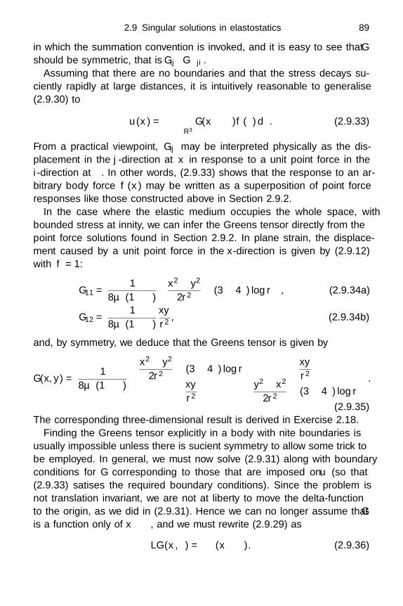
2.9 Singular solutions in elastostatics 89
in which the summation convention is invoked, and it is easy to see that Gshould be symmetric, that is Gij ≡ Gji.
Assuming that there are no boundaries and that the stress decays suffi-ciently rapidly at large distances, it is intuitively reasonable to generalise(2.9.30) to
u(x) =∫∫∫
R3G(x − ξ)f(ξ) dξ. (2.9.33)
From a practical viewpoint, Gij may be interpreted physically as the dis-placement in the j-direction at x in response to a unit point force in thei-direction at ξ. In other words, (2.9.33) shows that the response to an ar-bitrary body force f(x) may be written as a superposition of point forceresponses like those constructed above in Section 2.9.2.
In the case where the elastic medium occupies the whole space, withbounded stress at infinity, we can infer the Green’s tensor directly from thepoint force solutions found in Section 2.9.2. In plane strain, the displace-ment caused by a unit point force in the x-direction is given by (2.9.12)with f = 1:
G11 =1
8πµ(1 − ν)
(x2 − y2
2r2 − (3 − 4ν) log r
), (2.9.34a)
G12 =1
8πµ(1 − ν)xy
r2 , (2.9.34b)
and, by symmetry, we deduce that the Green’s tensor is given by
G(x, y) =1
8πµ(1 − ν)
x2 − y2
2r2 − (3 − 4ν) log rxy
r2
xy
r2y2 − x2
2r2 − (3 − 4ν) log r
.
(2.9.35)The corresponding three-dimensional result is derived in Exercise 2.18.
Finding the Green’s tensor explicitly in a body with finite boundaries isusually impossible unless there is sufficient symmetry to allow some trick tobe employed. In general, we must now solve (2.9.31) along with boundaryconditions for G corresponding to those that are imposed on u (so that(2.9.33) satisfies the required boundary conditions). Since the problem isnot translation invariant, we are not at liberty to move the delta-functionto the origin, as we did in (2.9.31). Hence we can no longer assume that Gis a function only of x − ξ, and we must rewrite (2.9.29) as
LG(x, ξ) = −δ(x − ξ). (2.9.36)
90 Linear elastostatics
We note that the full-space Green’s tensor, which is (2.9.35) in planestrain, can be used to reduce the Navier equation on an arbitrary domainD to an integral equation satisfied on the boundary of D. This reduction indimension can facilitate an efficient numerical solution, and forms the basisof the boundary element method. To illustrate the basic ideas behind thismethod, we begin by recalling the identities∫∫∫
D
(u · ∇2v − v · ∇2u
)dx =
∫∫∂D
(u · ∂v
∂n− v · ∂u
∂n
)dS (2.9.37)
and∫∫∫Du · (grad div v) − v · (grad div u) dx
=∫∫
∂D(div v) u · n − (div u)v · n dS, (2.9.38)
for any pair of vector fields u and v.Now, reluctantly reverting to suffix notation, we know that
(λ + µ) grad div Gij + µ∇2Gij = −δ(x − ξ) δij , (2.9.39)
(λ + µ) (grad div u)j + µ∇2uj =∂τjk
∂xk= 0, (2.9.40)
where we have neglected the body force for simplicity. Hence, multiplying(2.9.39) by ui, (2.9.40) by Gij , then subtracting and integrating, we find that
ui(ξ) =∫∫
∂D
Gi(x − ξ) · (τn (x)) − u(x) ·
(τ in(x − ξ)
)dS, (2.9.41)
where Gi = (Gi1,Gi2,Gi3)T and τ i is the stress field associated with the
displacement Gi.Hence, given the traction and displacement on the boundary ∂D, we have
an explicit representation of u everywhere in D. However, we do not expectboth u and τn to be given simultaneously on the boundary, so let us assumefor example that the surface traction τn is prescribed. In this case, (2.9.41)becomes an integral equation for u(ξ) as ξ tends to the boundary of theelastic solid. To solve this integral equation rather than the Navier equationnumerically is the basic idea behind the boundary element method. Thisapproach may prove advantageous compared to the more commonly usedfinite element method, since only the boundary of the solid needs to bediscretised, rather than the whole body. On the other hand, it also bringsits own share of difficulties. For example, the matrices resulting from thediscretisation are usually full, and care must be taken with the singularitiesthat occur in Gi as ξ approaches ∂D.
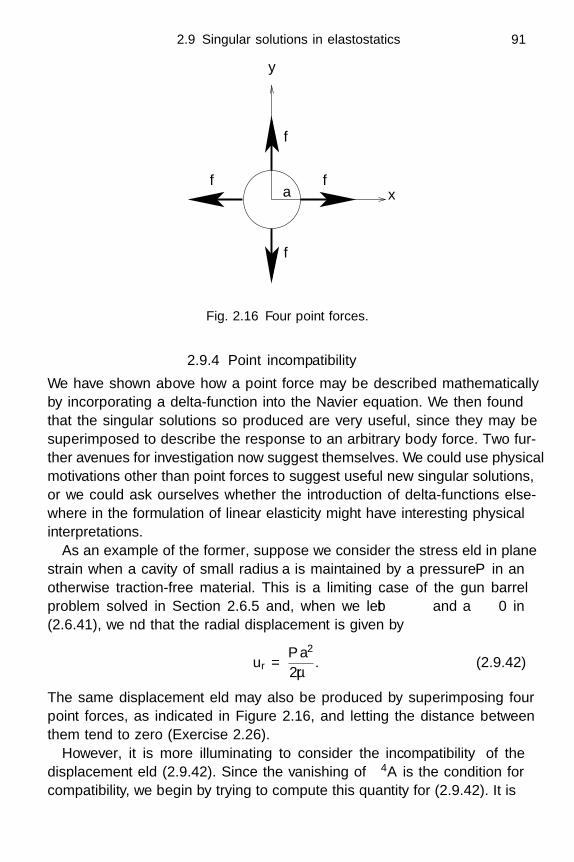
2.9 Singular solutions in elastostatics 91
x
y
f f
f
f
a
Fig. 2.16 Four point forces.
2.9.4 Point incompatibility
We have shown above how a point force may be described mathematicallyby incorporating a delta-function into the Navier equation. We then foundthat the singular solutions so produced are very useful, since they may besuperimposed to describe the response to an arbitrary body force. Two fur-ther avenues for investigation now suggest themselves. We could use physicalmotivations other than point forces to suggest useful new singular solutions,or we could ask ourselves whether the introduction of delta-functions else-where in the formulation of linear elasticity might have interesting physicalinterpretations.
As an example of the former, suppose we consider the stress field in planestrain when a cavity of small radius a is maintained by a pressure P in anotherwise traction-free material. This is a limiting case of the gun barrelproblem solved in Section 2.6.5 and, when we let b → ∞ and a → 0 in(2.6.41), we find that the radial displacement is given by
ur =Pa2
2µr. (2.9.42)
The same displacement field may also be produced by superimposing fourpoint forces, as indicated in Figure 2.16, and letting the distance betweenthem tend to zero (Exercise 2.26).
However, it is more illuminating to consider the incompatibility of thedisplacement field (2.9.42). Since the vanishing of ∇4A is the condition forcompatibility, we begin by trying to compute this quantity for (2.9.42). It is
92 Exercises
easy to see that A = −a2P log r and hence, using (2.9.7), that
∇2A = −2πa2Pδ(x)δ(y). (2.9.43)
Thus the incompatibility associated with the displacement field (2.9.42) isgiven by
∇4A = −2πa2P(δ′′(x)δ(y) + δ(x)δ′′(y)
), (2.9.44)
where, by analogy with (2.9.3), the derivative of a delta-function can bedefined by ∫ ∞
−∞δ′(x − ξ)ψ(ξ) dξ = ψ′(x) (2.9.45)
for any suitably smooth test function ψ. Hence (2.9.42) satisfies the compat-ibility relations everywhere except at the origin, where the localised sourceof incompatibility is known as a nucleus of strain (Love, 1944, Article 132).Note that no traction need be applied away from the origin to maintain thestress field associated with (2.9.42), and the material is therefore said to bein a state of self-stress.
More generally, in Exercise 2.21 it is shown that the compatibility condi-tions (2.7.5) are the six components of the symmetric tensor equation
ηij = εiklεjmn∂2emk
∂xn∂xl≡ 0, (2.9.46)
where εijk is the alternating symbol and we sum over k, l, m and n. Wetherefore define ηij as the incompatibility tensor. In plane strain, for example,the zz-component of (2.9.46) is
∂2exx
∂y2 − 2∂2exy
∂x∂y+
∂2eyy
∂x2 =1 − ν
2µ∇4A = 0, (2.9.47)
which reproduces (2.7.5a) and shows explicitly how ∇4A is related to com-patibility. Thus the right-hand side of (2.9.44) can be thought of as a pointsingularity in the incompatibility tensor, and this prompts us to wonder whatthe physical significance might be of introducing other point singularities onthe right-hand side of (2.9.46). For example, the physical interpretation ofsolutions of
∂2exx
∂y2 − 2∂2exy
∂x∂y+
∂2eyy
∂x2 = δ(x)δ′(y) (2.9.48)
has fundamental implications for the theory of metal plasticity, to which wewill return in Chapter 8.

2.10 Concluding remark 93
2.10 Concluding remark
All the solutions in this chapter were derived for purely static situations but,in fact, they also apply to unsteady problems that evolve on a sufficientlylong time-scale. For example, the analysis of a statically loaded torsion barcarried out in Section 2.4 applies equally well when the applied twist Ω is aslowly varying function of t. In such quasi-static situations, time appears inthe solution only as a parameter. This approach fails, however, to describeelastic waves, in which the displacement varies rapidly with time, and thetemporal and spatial dependence of the solution are coupled, as we will seein the following chapter.
Exercises
2.1 Use strips of stiff paper and sticky tape to construct the model shownin Figure 2.3(a). Now when you pull it in the direction shown, itexpands in the transverse direction, as indicated by Figure 2.3(b). Ittherefore has negative Poisson’s ratio.
2.2 An elastic membrane is stretched to an isotropic tension T such thatits height is given by z = w(x, y). Assuming that the membrane isnearly horizontal (so that |∇w| 1), show that T must be spatiallyuniform and that w must satisfy Laplace’s equation.
2.3 A uniform cylindrical bar is held with its axis along the z-axis andits boundary pinned. If the gravitational acceleration g acts in the−z direction, show that the vertical displacement w(x, y) satisfies
∇2w =ρg
µ
in the cross-section D of the bar, with w = 0 on ∂D.2.4 If D is the ellipse x2/a2 + y2/b2 < 1, show that the solution of
(2.4.12), (2.4.13) is
φ =a2b2
(a2 + b2)
(1 − x2
a2 − y2
b2
).
Hence show that the torsional rigidity of a bar with uniform ellipticalcross-section is
T =πµa3b3
a2 + b2 .
Deduce that a circular bar has a higher rigidity than an ellipticalbar with the same cross-sectional area.

94 Linear elastostatics
2.5 Derive the expression (2.5.2) for the torsional rigidity of a tubularbar. By contour deformation show that, if (2.5.3) holds when C is∂Di, then it holds for all simple closed paths C contained in D.
2.6 By separating the variables in polar coordinates, show that the prob-lem (2.5.14) for a cut tubular bar has the solution
φ =b2 − r2
2+
(b2 − a2
)log (r/b)
2 log (b/a)
+∞∑
n=1
Cn cosh[kn(θ − π)
]sin[kn log (b/r)
],
where
kn =nπ
log (b/a), Cn = −
4[b2 − (−1)na2
]log2 (b/a)
nπ cosh(knπ)[n2π2 + 4 log2 (b/a)
] .Use (2.4.15) to determine the torsional rigidity
R =πµ
(b2 − a2
)2 log (b/a)
[(a2 + b2) log (b/a) −
(b2 − a2)]
− 16µ log4 (b/a)π
∞∑n=1
[b2 − (−1)na2
]tanh
[nπ2/ log (b/a)
][n2π2 + 4 log2 (b/a)
]2 .
Now suppose that the tube is thin, so that b/a = 1+ε, where ε 1.By expanding the above expression for small ε, show that
R =2π
3µa4ε3
1 −
(12
+93ζ(5)
π6
)ε + · · ·
,
where ζ is the Riemann zeta function (Abramowitz & Stegun, 1972,Section 23.2).
2.7 If z = x + iy and z = x − iy are regarded as independent variables,show that
∇2ψ = 4∂2ψ
∂z∂z.
Deduce that the general solution of Laplace’s equation may be writ-ten in the form
ψ =12f(z) + h(z),
where f and h are arbitrary analytic functions. If ψ takes only realvalues, show that h(z) = f(z) and hence that
ψ = Ref(z)
.
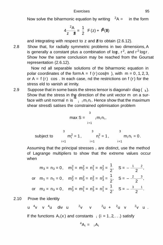
Exercises 95
Now solve the biharmonic equation by writing ∇2A = ψ in the form
4∂2A
∂z∂z=
12F (z) + F (z)
and integrating with respect to z and z to obtain (2.6.12).
2.8 Show that, for radially symmetric problems in two dimensions, A
is generally a constant plus a combination of log r, r2, and r2 log r.Show how the same conclusion may be reached from the Goursatrepresentation (2.6.12).
Now find all separable solutions of the biharmonic equation inpolar coordinates of the form A = f(r) cos(mθ), with m = 0, 1, 2, 3,or A = f(r)θ cos θ. In each case, find the restrictions on f(r) for thestress field to vanish at infinity.
2.9 Suppose that in some basis the stress tensor is diagonal: τ = diag (τk).Show that the stress in the direction of the unit vector m on a sur-face with unit normal n is
∑i τimini. Hence show that the maximum
shear stress S satisfies the constrained optimisation problem
max S =3∑
i=1
τimini,
subject to3∑
i=1
m2i = 1,
3∑i=1
n2i = 1,
3∑i=1
mini = 0.
Assuming that the principal stresses τi are distinct, use the methodof Lagrange multipliers to show that the extreme values occurwhen
m3 = n3 = 0, m21 = m2
2 = n21 = n2
2 =12, S = ±τ1 − τ2
2,
or m1 = n1 = 0, m22 = m2
3 = n22 = n2
3 =12, S = ±τ2 − τ3
2,
or m2 = n3 = 0, m23 = m2
1 = n23 = n2
1 =12, S = ±τ3 − τ1
2.
2.10 Prove the identity
u∇4v − v∇4u ≡ divu∇
(∇2v
)− v∇
(∇2u
)+ ∇2u∇v −∇2v∇u
.
If the functions Ai(x) and constants λi (i = 1, 2, . . .) satisfy
∇4Ai = λiAi

96 Linear elastostatics
in some bounded region V , show that
(λi − λj)∫∫∫
VAiAj dx =
∫∫∂V
∇2Aj
∂Ai
∂n−∇2Ai
∂Aj
∂n
+ Aj∂
∂n
(∇2Ai
)− Ai
∂
∂n
(∇2Aj
)dS.
Deduce that the biharmonic operator has real eigenvalues and or-thogonal eigenfunctions when the boundary conditions are
(i) A =∂A
∂n= 0, or (ii) A = ∇2A = 0,
or (iii)∂A
∂n=
∂
∂n
(∇2A
), or (iv) ∇2A =
∂
∂n
(∇2A
)= 0.
2.11 (a) Assuming y > 0, show that the inverse Fourier transforms ofe−|k|y and i sign(k)e−y|k| are given by
f1(x, y) =12π
∫ ∞
−∞e−ikxe−|k|y dk =
y
π (x2 + y2),
and
f2(x, y) =i
2π
∫ ∞
−∞e−ikx sign(k)e−|k|y dk =
x
π (x2 + y2),
respectively.(b) Hence show that (2.6.79) may be written as
τxx = −P (k)(
1 + y∂
∂y
)f1(k, y),
τxy = P (k)y∂f1
∂x(k, y),
τyy = −P (k)(
1 − y∂
∂y
)f1(k, y).
Using the fact that the inverse Fourier transform of a productf(k)g(k) is the convolution of f and g, that is
(f ∗ g)(x) =∫ ∞
−∞f(x − s)g(s) ds,
deduce (2.6.80).(c) Show from (2.6.82) that
2µ∂v
∂x= P (k)
(y∂f1
∂x(k) − 2(1 − ν)f2(k)
),
and hence deduce (2.6.83).

Exercises 97
2.12 By making a suitable substitution, write the second term in theintegral (2.6.83) as
−(2 − ν)y2
π
∫ ∞
−∞
P (x − s)sds
(s2 + y2)2 = −2 − ν
π
∫ ∞
−∞
P (x − yt)t dt
(1 + t2)2 .
Deduce that, provided P (x) is bounded, this term tends to zero asy → 0.
Show further that the first term in (2.6.83) may be written as
−1 − ν
π
(∫ −ε
−∞+∫ ε
−ε+∫ ∞
ε
)P (s)(x − s)3 ds
((x − s)2 + y2)2 .
Show that the middle integral is approximately equal to
−(1 − ν)P (x)π
∫ ε/y
−ε/y
t3 dt
(1 + t2)2 ,
and explain why this integral tends to zero as y tends to zero withy ε 1. Finally deduce that, as y → 0, (2.6.83) tends to (2.6.85),where the Hilbert transform is defined by
H[P ](x) =1π−∫ ∞
−∞
P (s) ds
s − x=
1π
limε↓0
(∫ −ε
−∞+∫ ∞
ε
)P (s) ds
s − x.
2.13 Show that, if ∇2φ = 0 in the half-space y > 0 with φ(x, 0) = f(x),∂φ/∂y(x, 0) = g(x) and φ → 0 at infinity, then
φ =12π
∫ ∞
−∞g(s) log
[(s − x)2 + y2
]ds.
Deduce that f ′(x) = ∂φ/∂x(x, 0) = −H[g].Show further that ∂2φ/∂y2(x, 0) = −f ′′(x), so that
∂φ
∂y= − 1
2π
∫ ∞
−∞f ′′(s) log
[(s − x)2 + y2
]ds.
Hence deduce that g(x) = H[f ′].2.14 Reconsider the torsion problem of Section 2.4 and the stress function
φ defined by (2.4.10). Using two of the compatibility relations (2.7.5),deduce successively that ∇2φ = f(y), that ∇2φ = g(x), and hencethat ∇2φ = const..
[This illustrates that two compatibility conditions that are not inde-pendent may nevertheless both be necessary to determine the stress.]

98 Linear elastostatics
2.15 (a) Derive the expression (2.6.97) for the modified Airy stressfunction outside a circular underground tunnel.
(b) Prove the identity
∂2ur
∂θ2 + ur = −r2 ∂eθθ
∂r+ rerr + 2r
∂erθ
∂θ(E2.1)
relating the strain components to the radial displacement ur
in plane polar coordinates (r, θ). Deduce that the coefficientsof sin θ and cos θ on the right-hand side must be zero if ur isto be a 2π-periodic function of θ.
(c) With the stress components given by (2.6.92), show that theright-hand side of (E2.1) is
−ρgh
(a2
r+ (1 − 2ν)r
)+(
8(1 − ν)A1 + 2 log a
)cos θ
+(
8(1 − ν)B1 + 2 log a
− ρg(1 − 2ν)a2)
sin θ,
and hence obtain the expressions (2.6.98).2.16 Return to the tunnel example of Section 2.6.9, this time assuming a
far-field stress distribution given by τxx = τxy = 0, τyy = ρg(y −H).[This might correspond to a cylindrical hole in a vertical column.]In this case, show that (2.6.92) becomes
τrr = ρg sin2 θ (r sin θ − H) +1r2
∂2A
∂θ2 +1r
∂A
∂r,
τrθ = ρgsin 2θ
2(r sin θ − H) − ∂
∂r
(1r
∂A
∂θ
),
τθθ = ρg cos2 θ (r sin θ − H) +∂2A
∂r2 ,
and that the boundary conditions on r = a are
A(a, θ) =ρga2
2
(H + aθ cos θ +
H
2cos 2θ − a
12sin 3θ
)+ A cos θ + B sin θ,
∂A
∂r(a, θ) =
ρga
2
(H + aθ cos θ + H cos 2θ − a
4sin 3θ
)+
A
acos θ +
B
asin θ,

Exercises 99
where A and B are arbitrary constants. Use (E2.1) and the fact thatur is single-valued to show that
A = 0, B = −νρga3/4,
so that
A =ρga2
2
H(1 + log
r
a
)+ rθ cos θ + H
(1 − a2
2r2
)cos 2θ
+12
(r(1 − 2ν) log
r
a− a2
r
)sin θ +
(a4
6r3 − a2
4r
)sin 3θ
,
and deduce that the hoop stress is given by
τθθ = −ρgH (1 + 2 cos 2θ) + ρga
(1 − 2ν
2sin θ + sin 3θ
)on r = a. Note the contrast with the stress distribution (2.6.100)caused by a hydrostatic far-field stress.
2.17 By comparing (2.6.9) and (2.8.22), show that z-averaged plane stressis mathematically equivalent to plane strain with new elastic con-stants ν ′ and E′ given by
ν ′ =ν
1 + ν, E′ =
1 + 2ν
(1 + ν)2 E.
2.18 We define the three-dimensional Fourier transform of a functionf(x, y, z) by
f =∫ ∞
−∞
∫ ∞
−∞
∫ ∞
−∞f(x, y, z)ei(kx+y+mz) dxdydz
=∫∫∫
R3f(x)ei(k·x) dx,
where k = (k, , m). Show that the Fourier transform of the Green’stensor in three dimensions is given by
G =(Gij
)=
1µ|k|2 I − λ + µ
µ (λ + 2µ)kkT
|k|4 ,
and, by inverting the transform, deduce that
Gij =λ + µ
8πµ (λ + 2µ)1|x|
(λ + 3µ
λ + µδij +
xixj
|x|2)
. (E2.2)
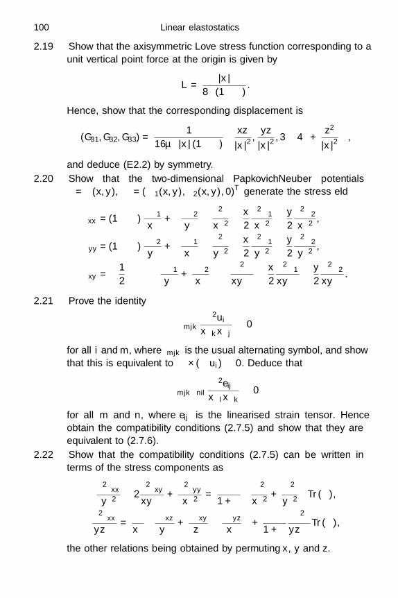
100 Linear elastostatics
2.19 Show that the axisymmetric Love stress function corresponding to aunit vertical point force at the origin is given by
L =|x|
8π (1 − ν).
Hence, show that the corresponding displacement is
(G31,G32,G33) =1
16πµ |x| (1 − ν)
(xz
|x|2,
yz
|x|2, 3 − 4ν +
z2
|x|2)
,
and deduce (E2.2) by symmetry.2.20 Show that the two-dimensional Papkovich–Neuber potentials
φ = φ(x, y), Ψ = (ψ1(x, y), ψ2(x, y), 0)T generate the stress field
τxx = (1 − ν)∂ψ1
∂x+ ν
∂ψ2
∂y− ∂2φ
∂x2 − x
2∂2ψ1
∂x2 − y
2∂2ψ2
∂x2 ,
τyy = (1 − ν)∂ψ2
∂y+ ν
∂ψ1
∂x− ∂2φ
∂y2 − x
2∂2ψ1
∂y2 − y
2∂2ψ2
∂y2 ,
τxy =(
12− ν
)(∂ψ1
∂y+
∂ψ2
∂x
)− ∂2φ
∂x∂y− x
2∂2ψ1
∂x∂y− y
2∂2ψ2
∂x∂y.
2.21 Prove the identity
εmjk∂2ui
∂xk∂xj≡ 0
for all i and m, where εmjk is the usual alternating symbol, and showthat this is equivalent to ∇×(∇ui) ≡ 0. Deduce that
εmjkεnil∂2eij
∂xl∂xk≡ 0
for all m and n, where eij is the linearised strain tensor. Henceobtain the compatibility conditions (2.7.5) and show that they areequivalent to (2.7.6).
2.22 Show that the compatibility conditions (2.7.5) can be written interms of the stress components as
∂2τxx
∂y2 − 2∂2τxy
∂x∂y+
∂2τyy
∂x2 =ν
1 + ν
(∂2
∂x2 +∂2
∂y2
)Tr (τ),
∂2τxx
∂y∂z=
∂
∂x
(∂τxz
∂y+
∂τxy
∂z− ∂τyz
∂x
)+
ν
1 + ν
∂2
∂y∂zTr (τ),
the other relations being obtained by permuting x, y and z.

Exercises 101
2.23 Verify (2.9.7a) by writing |x| = limε→0√
x2 + ε2 and noting that
d2
dx2
(√x2 + ε2
)=
ε2
(x2 + ε2)3/2 ,
and ∫ ∞
−∞
ε2 dx
(x2 + ε2)3/2 =∫ ∞
−∞
ds
(1 + s2)3/2 = 2.
Repeat this procedure with log(x2 + y2 + ε2
)to derive (2.9.7b) and
find a similar derivation of (2.9.7c).2.24 Show that(
∂2
∂x2 +∂2
∂y2
)[(x2 + y2) log
(x2 + y2)] = 8 + 4 log
(x2 + y2)
and deduce that, if A = (1/8π)(x2 + y2
)log
(x2 + y2
), then A satis-
fies
∇4A = δ(x)δ(y).
2.25 The stress components due to a point force f in the x-directionsatisfy
∂τxx
∂x+
∂τxy
∂y= −fδ(x)δ(y),
∂τxy
∂x+
∂τyy
∂y= 0
plus the compatibility condition
∂2τxx
∂y2 − 2∂2τxy
∂x∂y+
∂2τyy
∂x2 − ν∇2 (τxx + τyy) = 0.
Take a two-dimensional Fourier transform (defined as in Exercise 2.18)to show that
kτxx + τxy = −if, kτxy + τyy = 0,
−2 τxx + 2kτxy − k2 τyy + ν(k2 + 2) (τxx + τyy) = 0.
Hence obtain
τxx =ikf
1 − ν
(ν
k2 + 2 − k2 + 22
(k2 + 2)2
),
τxy =if
1 − ν
(ν
k2 + 2 − 2
(k2 + 2)2
),
τyy =−ikf
1 − ν
(ν
k2 + 2 − 2
(k2 + 2)2
),
the inverse Fourier transform of which is (2.9.13).
102 Linear elastostatics
2.26 Write down the displacement field for the four point forces depictedin Figure 2.16. Let a → 0 and show that the displacement tends to
u =1 − 2ν
1 − ν
af
2πµ
er
r,
which agrees with (2.9.42) if f = πa(1 − ν)/(1 − 2ν).
3
Linear elastodynamics
3.1 Introduction
This chapter concerns simple unsteady problems in linear elasticity. As notedin Section 1.10, the unsteady Navier equation (1.7.8) bears some similarity tothe familiar scalar wave equation governing small transverse displacementsof an elastic string or membrane. We therefore start by reviewing the mainproperties of this equation and some useful solution techniques. This allowsus to introduce, in a simple context, important concepts such as normalmodes, plane waves and characteristics that underpin most problems inlinear elastodynamics.
In contrast with the classical scalar wave equation, the Navier equation isa vector wave equation, and this introduces many interesting new properties.The first that we will encounter is that the Navier equation in an infinitemedium supports two distinct kinds of plane waves which propagate at twodifferent speeds. These are known as P -waves and S -waves, and correspondto compressional and shearing oscillations of the medium respectively. Con-sidered individually, both P - and S -waves behave very much like waves asmodelled by the scalar wave equation (1.10.9). In practice, though, theyvery rarely exist in isolation since any boundaries present inevitably convertP -waves into S -waves and vice versa. We will illustrate this phenomenon ofmode conversion in Section 3.2.5 by considering the reflection of waves at aplane boundary.
In two-dimensional and axisymmetric problems, we found in Chapter 2that the steady Navier equation may be transformed into a single biharmonicequation by introducing a suitable stress function. In Sections 3.3 and 3.4we will find that the same approach often works even for unsteady problems,and pays dividends when we come to analyse normal modes in cylinders andspheres.
103

104 Linear elastodynamics
In Section 3.5, we consider some initial-value problems for elastic wavepropagation using the ideas of characteristics and fundamental solutions.Finally, we will discuss the interesting phenomena that can occur whenelastic waves are generated by moving sources.
Before we begin, let us briefly recall some familiar wave propagation mod-els for elastic strings and membranes. The simplest such model describessmall oscillations of an elastic string of line density under a tension T . Itis well known that the transverse displacement w (x, t) satisfies the partialdifferential equation
∂2w
∂t2= T
∂2w
∂x2 , (3.1.1)
known as the one-dimensional wave equation. The derivation and validity ofthis equation will be discussed in Chapter 4, where we will show that it alsodescribes longitudinal waves in an elastic bar.
If we instead consider an elastic membrane with surface density ς stretchedacross the (x, y)-plane under a uniform tension T , then the appropriategeneralisation of (3.1.1) is
ς∂2w
∂t2= T∇2w, (3.1.2)
where ∇2 = ∂2/∂x2 + ∂2/∂y2 is the two-dimensional Laplacian. The three-dimensional version of (3.1.2) governs many familiar wave propagation prob-lems including acoustic waves and light waves.
There are two ways in which we can approach (3.1.1) and (3.1.2) mathe-matically. One possibility is to try to construct a general solution that willapply whatever mechanism is driving the waves. However, this strategy isonly useful in practice when the general solution can be found explicitlyand also takes a sufficiently simple form for realistic boundary conditionsto be imposed. Alternatively, we can attempt to describe the solution asa linear combination of elementary solutions, as in the method of normalmodes in classical mechanics. This second approach can always be appliedin principle and ties in with the first when we view the general solution as asuperposition of elementary solutions. We therefore begin the next sectionby discussing some elementary solutions of (3.1.1) and (3.1.2).
3.2 Normal modes and plane waves
3.2.1 Normal modes
A normal mode of a dynamical system is a motion in which the whole systemoscillates at a single frequency ω. We can seek normal modes of an elastic
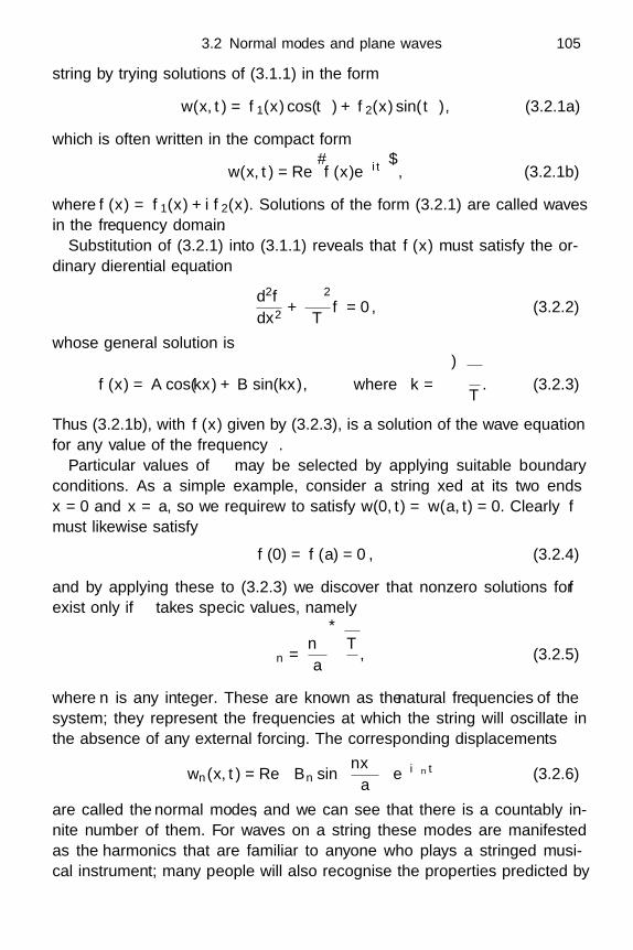
3.2 Normal modes and plane waves 105
string by trying solutions of (3.1.1) in the form
w(x, t) = f1(x) cos(ωt) + f2(x) sin(ωt), (3.2.1a)
which is often written in the compact form
w(x, t) = Re[f(x)e−iωt
], (3.2.1b)
where f(x) = f1(x) + if2(x). Solutions of the form (3.2.1) are called wavesin the frequency domain.
Substitution of (3.2.1) into (3.1.1) reveals that f(x) must satisfy the or-dinary differential equation
d2f
dx2 +ω2
Tf = 0, (3.2.2)
whose general solution is
f(x) = A cos(kx) + B sin(kx), where k = ω
√
T. (3.2.3)
Thus (3.2.1b), with f(x) given by (3.2.3), is a solution of the wave equationfor any value of the frequency ω.
Particular values of ω may be selected by applying suitable boundaryconditions. As a simple example, consider a string fixed at its two endsx = 0 and x = a, so we require w to satisfy w(0, t) = w(a, t) = 0. Clearly f
must likewise satisfy
f(0) = f(a) = 0, (3.2.4)
and by applying these to (3.2.3) we discover that nonzero solutions for f
exist only if ω takes specific values, namely
ωn =nπ
a
√T
, (3.2.5)
where n is any integer. These are known as the natural frequencies of thesystem; they represent the frequencies at which the string will oscillate inthe absence of any external forcing. The corresponding displacements
wn(x, t) = Re(Bn sin
(nπx
a
)e−iωn t
)(3.2.6)
are called the normal modes, and we can see that there is a countably in-finite number of them. For waves on a string these modes are manifestedas the harmonics that are familiar to anyone who plays a stringed musi-cal instrument; many people will also recognise the properties predicted by
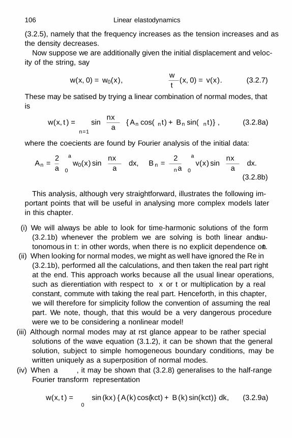
106 Linear elastodynamics
(3.2.5), namely that the frequency increases as the tension increases and asthe density decreases.
Now suppose we are additionally given the initial displacement and veloc-ity of the string, say
w(x, 0) = w0(x),∂w
∂t(x, 0) = v(x). (3.2.7)
These may be satisfied by trying a linear combination of normal modes, thatis
w(x, t) =∞∑
n=1
sin(nπx
a
)An cos(ωnt) + Bn sin(ωnt) , (3.2.8a)
where the coefficients are found by Fourier analysis of the initial data:
An =2a
∫ a
0w0(x) sin
(nπx
a
)dx, Bn =
2ωna
∫ a
0v(x) sin
(nπx
a
)dx.
(3.2.8b)
This analysis, although very straightforward, illustrates the following im-portant points that will be useful in analysing more complex models laterin this chapter.
(i) We will always be able to look for time-harmonic solutions of the form(3.2.1b) whenever the problem we are solving is both linear and au-tonomous in t: in other words, when there is no explicit dependence on t.
(ii) When looking for normal modes, we might as well have ignored the “Re” in(3.2.1b), performed all the calculations, and then taken the real part rightat the end. This approach works because all the usual linear operations,such as differentiation with respect to x or t or multiplication by a realconstant, commute with taking the real part. Henceforth, in this chapter,we will therefore for simplicity follow the convention of assuming the realpart. We note, though, that this would be a very dangerous procedurewere we to be considering a nonlinear model!
(iii) Although normal modes may at first glance appear to be rather specialsolutions of the wave equation (3.1.2), it can be shown that the generalsolution, subject to simple homogeneous boundary conditions, may bewritten uniquely as a superposition of normal modes.
(iv) When a → ∞, it may be shown that (3.2.8) generalises to the half-rangeFourier transform representation
w(x, t) =∫ ∞
0sin (kx) A(k) cos(kct) + B(k) sin(kct)dk, (3.2.9a)

3.2 Normal modes and plane waves 107
where c2 = T/ and
A(k) =2π
∫ ∞
0w0(x) sin(kx) dx, B(k) =
2πkc
∫ ∞
0v(x) sin(kx) dx.
(3.2.9b)
We can extend these ideas to the two-dimensional wave equation (3.1.2)by seeking solutions of the form
w(x, y, t) = A(x, y)e−iωt, (3.2.10)
and we find that A must satisfy the Helmholtz equation
∇2A + k2A = 0, (3.2.11)
where k = ω√
ς/T . For example, to find the normal modes and frequenciesof a drum whose skin occupies a region D in the (x, y)-plane, we mustsolve (3.2.11) in D subject to A = 0 on the boundary ∂D. This is anothereigenvalue problem: A ≡ 0 is always a possible solution and special valuesof k must be sought such that A may be nonzero. For many simple shapes,these can be found by separating the variables. For example, we can see ata glance that the normal modes and natural frequencies of the rectangularmembrane 0 < x < a, 0 < y < b are
wm,n(x, y, t) = sin(mπx
a
)sin
(nπy
b
)e−iωm ,n t, (3.2.12a)
ω2m,n =
π2T
ς
(m2
a2 +n2
b2
), (3.2.12b)
where m and n are arbitrary integers. Thus there is a doubly infinite set ofnormal modes in this case. In general, there is one infinite set of frequenciesfor each spatial dimension in the problem.
Next we consider radially-symmetric vibrations of a circular drum, so thatA is a function of the plane polar distance r and (3.2.11) reads
d2A
dr2 +1r
dA
dr+ k2A = 0, (3.2.13a)
to be solved subject to A(a) = 0. If we set ξ = kr, then the problem for A
becomes
d2A
dξ2 +1ξ
dA
dξ+ A = 0 with A(ka) = 0. (3.2.13b)
This is Bessel’s equation of order zero, and it is easy to see that A(ξ) os-cillates for large ξ, because the first and last terms in (3.2.13) will be ap-proximately in balance. Moreover, for small ξ, we can spot that the first and

108 Linear elastodynamics
5 10 15 20 25 30
-0.4
-0.2
0.2
0.4
0.6
0.8
1
5 10 15 20 25 30
-0.8
-0.6
-0.4
-0.2
0.2
0.4
ξ
ξ
Jn(ξ)
Yn(ξ)
2
2
n = 0
1
1n = 0
Fig. 3.1 Plots of the first three Bessel functions Jn (ξ) and Yn (ξ) for n = 0 (solid),n = 1 (dashed), n = 2 (dot-dashed).
second terms in (3.2.13) both balance and dominate the third term whenA = log ξ. This suggests that the solution is either well-behaved or loga-rithmically singular as ξ → 0, and this conclusion may easily be confirmedusing Frobenius’ method. The bounded solution with A(0) = 1 is denotedby J0(ξ) while the singular solution with A ∼ (2/π) log ξ is called Y0(ξ), andthese important functions are plotted in Figure 3.1.
Here, we require the amplitude A to be bounded at the centre of the drumr = 0 and must therefore choose A = const. J0(ξ). The condition at r = a isthen satisfied if
ka = ξ0,i (i = 1, 2, . . .), (3.2.14a)
where ξ0,1 < ξ0,2 < · · · are the zeros of J0(ξ). As indicated in Figure 3.1,there are an infinite number of these zeros and ξ0,n → ∞ as n → ∞. Thenatural frequencies of the drum for radially-symmetric modes are thus given

3.2 Normal modes and plane waves 109
by
ωi =ξ0,i
a
√T
ς(n = 1, 2, . . .). (3.2.14b)
Unlike the modes on a string, the natural frequencies here are irrationalmultiples of each other. In musical terms, the harmonics are out of tunewith each other, and this gives rise to the characteristic sound of a drum,which is quite different from that of a piano or a violin, for example.
If we drop the assumption of radial symmetry, then the Helmholtz equa-tion becomes
∂2A
∂r2 +1r
∂A
∂r+
1r2
∂2A
∂θ2 + k2A = 0, (3.2.15)
in plane polar coordinates (r, θ). Again we impose A = 0 on r = a, and nowwe insist also that A must be a 2π-periodic function of θ. This restricts usto seeking separable solutions of the form
A(r, θ) = f(r)(C1 cos(nθ) + C2 sin(nθ)
), (3.2.16)
where n is an integer, and it follows that f satisfies
r2 d2f
dr2 + rdf
dr+(k2r2 − n2) f = 0 with f(a) = 0. (3.2.17a)
Setting ξ = kr as before, we find that (3.2.17a) becomes
ξ2 d2f
dξ2 + ξdf
dξ+(ξ2 − n2) f = 0 with f(ka) = 0. (3.2.17b)
This is Bessel’s equation of order n, whose two linearly dependent so-lutions are denoted Jn(ξ) and Yn(ξ); the cases n = 0, 1, 2 are plotted inFigure 3.1. For any integer n, Yn(ξ) is singular as ξ → 0, so we must choosef = const. Jn(ξ). The condition at r = a is then satisfied if
ka = ξn,i (i = 1, 2, . . .), (3.2.18)
where ξn,1 < ξn,2 < · · · are the zeros of Jn(ξ). There are an infinite numberof these zeros and ξn,i → ∞ as i → ∞. The natural frequencies of the drumare thus given by
ω2n,i =
ξ2n,iT
a2ς, (3.2.19)
where n and i are arbitrary integers, so there is a doubly-infinite family ofnormal modes that depend on the two spatial coordinates (r, θ).

110 Linear elastodynamics
3.2.2 Plane waves
As suggested by (3.2.9), when looking for solutions of (3.1.1) on an infinitedomain, it is appropriate to seek travelling waves of the form
w(x, t) = A exp(i(kx − ωt)
), (3.2.20)
rather than seeking a discrete set of normal modes. The real constants |A|,k and ω represent the amplitude, wave-number and frequency, respectively,of the wave (3.2.20). The wave-number is related to the wave-length λ byk = 2π/λ, so large values of k correspond to short waves and vice versa. Wecan alternatively write (3.2.20) in the form
w(x, t) = A exp(ik(x − ct)
), where c =
ω
k; (3.2.21)
the quantity c is known as the phase velocity. From (3.2.21) we can easilysee that c represents the speed at which wave crests propagate. We can alsosee that the minus sign included by convention in (3.2.20) ensures that thewave propagates in the positive x-direction when ω and k are both positive.
We can generalise this approach to the two-dimensional wave equation(3.1.2) by looking for a plane wave solution of the form
w(x, y, t) = A exp(i(k1x + k2y − ωt)
)= A exp
(i(k · x − ωt
)), (3.2.22)
where we define the wave-vector k = (k1, k2)T. By writing (3.2.22) in theform
w = A exp(i(|k|X − ωt
)), where X =
k · x|k| , (3.2.23)
we observe that it represents a harmonic wave travelling in the directionof k at speed ω/|k|. The phase velocity, at which the wave crests propagate,is thus given by
c =ωk
|k|2 . (3.2.24)
When we substitute (3.2.20) into (3.1.1), we find that the amplitude canbe nonzero only if
ω2 = k2T/. (3.2.25a)
This dispersion relation tells us how the frequency of any given wave dependson its wave-length. We can also view (3.2.25a) as an equation for the phasevelocity, namely
c = ±√
T/, (3.2.25b)

3.2 Normal modes and plane waves 111
which tells us that all waves move at the same speed, irrespective of theirwave-length. Waves with this property are called non-dispersive, to distin-guish them from dispersive waves in which c varies with k.
Similarly, substitution of (3.2.22) into the two-dimensional wave equation(3.1.2) leads to the dispersion relation
ω2 = |k|2T/ς. (3.2.26)
The phase speed
|c| = c =√
T/ς (3.2.27)
is still independent of the wave-vector k, so these two-dimensional waves arealso non-dispersive.
As in (3.2.9), the general solution of the wave equation on an infinite do-main may be written as a linear superposition of harmonic waves, travellingin both directions, in the form of a Fourier integral. In other words, we canwrite
w(x, y, t) =∫ ∞
−∞
∫ ∞
−∞A(k1, k2) exp
i (k1x + k2y − ω(k1, k2)t)
+ B(k1, k2) exp
i (k1x + k2y + ω(k1, k2)t)
dk1dk2, (3.2.28a)
or
w(x, t) =∫∫
R2A(k) exp
i (k · x − ω(k)t)
+ B(k) exp
i (k · x + ω(k)t)
dk, (3.2.28b)
where ω(k) is given by the dispersion relation (3.2.26) and the amplitudefunctions A(k) and B(k) can be found from the Fourier transform of theinitial conditions. By writing the displacement in the form (3.2.28b), weindicate that this and all the other results in this section apply also to thewave equation in three space dimensions.
3.2.3 Scattering
Scattering refers generally to the problem of irradiating a target with aknown incoming wave-field and trying to determine the resultant scatteredfield that is the result of the presence of the target. This idea is important,for example, in tomography, seismology and ultrasonic testing, where we tryto infer, non-invasively, the properties of some inhomogeneities in a bulkelastic medium by measuring the scattered wave-fields that they produce.
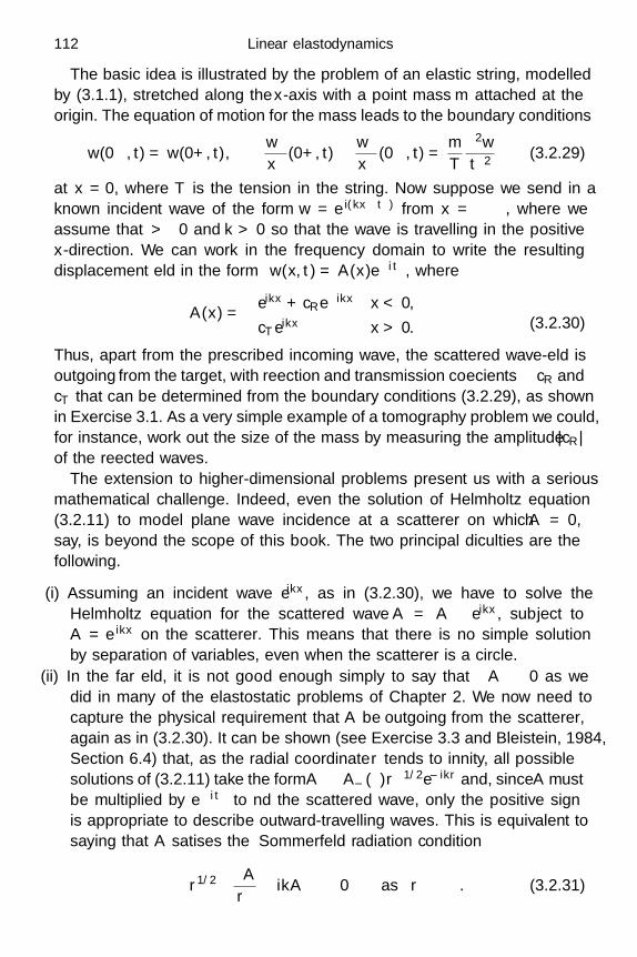
112 Linear elastodynamics
The basic idea is illustrated by the problem of an elastic string, modelledby (3.1.1), stretched along the x-axis with a point mass m attached at theorigin. The equation of motion for the mass leads to the boundary conditions
w(0−, t) = w(0+, t),∂w
∂x(0+, t) − ∂w
∂x(0−, t) =
m
T
∂2w
∂t2(3.2.29)
at x = 0, where T is the tension in the string. Now suppose we send in aknown incident wave of the form w = ei(kx−ωt) from x = −∞, where weassume that ω > 0 and k > 0 so that the wave is travelling in the positivex-direction. We can work in the frequency domain to write the resultingdisplacement field in the form w(x, t) = A(x)e−iωt, where
A(x) =
eikx + cRe−ikx x < 0,
cTeikx x > 0. (3.2.30)
Thus, apart from the prescribed incoming wave, the scattered wave-field isoutgoing from the target, with reflection and transmission coefficients cR andcT that can be determined from the boundary conditions (3.2.29), as shownin Exercise 3.1. As a very simple example of a tomography problem we could,for instance, work out the size of the mass by measuring the amplitude |cR|of the reflected waves.
The extension to higher-dimensional problems present us with a seriousmathematical challenge. Indeed, even the solution of Helmholtz’ equation(3.2.11) to model plane wave incidence at a scatterer on which A = 0,say, is beyond the scope of this book. The two principal difficulties are thefollowing.
(i) Assuming an incident wave eikx, as in (3.2.30), we have to solve theHelmholtz equation for the scattered wave A = A − eikx, subject toA = eikx on the scatterer. This means that there is no simple solutionby separation of variables, even when the scatterer is a circle.
(ii) In the far field, it is not good enough simply to say that A → 0 as wedid in many of the elastostatic problems of Chapter 2. We now need tocapture the physical requirement that A be outgoing from the scatterer,again as in (3.2.30). It can be shown (see Exercise 3.3 and Bleistein, 1984,Section 6.4) that, as the radial coordinate r tends to infinity, all possiblesolutions of (3.2.11) take the form A → A±(θ)r−1/2e±ikr and, since A mustbe multiplied by e−iωt to find the scattered wave, only the positive signis appropriate to describe outward-travelling waves. This is equivalent tosaying that A satisfies the Sommerfeld radiation condition
r1/2
(∂A
∂r− ikA
)→ 0 as r → ∞. (3.2.31)

3.2 Normal modes and plane waves 113
Then the canonical tomography problem for (3.2.11) is to reconstruct theshape of the scatterer given the directivity function A+(θ).
We note that, in the absence of any incident field, a circular boundary canradiate waves in which, from (3.2.16), A depends only on r and is a linearcombination of J0(kr) and Y0(kr). Using the fact that
J0(kr) ± iY0(kr) →√
2πkr
e±i(kr−(π/4)) as r → ∞, (3.2.32)
we see that, to describe outward-propagating waves, A must tend to a mul-tiple of the Hankel function H
(1)0 (kr) = J0(kr) + iY0(kr) as r → ∞.
3.2.4 P-waves and S-waves
Now we examine how the ideas developed above for scalar wave equationsmay be applied to the unsteady Navier equation (1.7.8). We begin by seekingtravelling-wave solutions in the form
u = a exp
i (k · x − ωt)
, (3.2.33)
where the complex amplitude a, the wave-vector k and frequency ω are allconstant. It is very helpful to use a little hindsight, or Exercise 3.4, to noticethat, for any vector a and nonzero k, there is a unique vector B and a scalarA satisfying
a = Ak + B×k, k · B = 0. (3.2.34)
Using this decomposition, we find that
∇2u = − |k|2 (Ak + B×k) exp
i (k · x − ωt)
, (3.2.35a)
grad div u = −A |k|2 k exp
i (k · x − ωt)
, (3.2.35b)
∂2u
∂t2= −ω2 (Ak + B×k) exp
i (k · x − ωt)
. (3.2.35c)
Hence the Navier equation (1.7.8) reduces to(ρω2 − µ|k|2
)(B×k) +
(ρω2 − (λ + 2µ)|k|2
)Ak = 0, (3.2.36)
which we can only satisfy for nonzero k if either
B = 0 and ρω2 = (λ + 2µ) |k|2 (3.2.37a)
or
A = 0 and ρω2 = µ |k|2 . (3.2.37b)

114 Linear elastodynamics
The vectorial nature of the Navier equation has thus led to the existence oftwo dispersion relations, corresponding to two distinct types of waves.
(i) P-waves, also known as Primary or Pressure waves, take the form
u = Ak exp
i (k · x − ωt)
, (3.2.38a)
where ω2 = (λ+2µ)|k|2/ρ. We recall from Section 1.9 that µ and λ+2µ/3are both positive, so ω is real. The phase speed is thus given by
cp =
√λ + 2µ
ρ(3.2.38b)
and, since cp is independent of k, the waves are non-dispersive. The phasevelocity
c =cpk
|k| (3.2.38c)
is parallel to the displacement u, so P -waves are said to be longitudi-nal. They are also sometimes described as irrotational since they satisfycurlu = 0, as is readily verified by direct differentiation of (3.2.38a).
(ii) S-waves, also known as Secondary or Shear waves, take the form
u = (B×k) exp
i (k · x − ωt)
, (3.2.39a)
where ω2 = µ|k|2/ρ. S -waves are also non-dispersive, with constant phasespeed
cs =√
µ
ρ. (3.2.39b)
This time, though, the phase velocity is perpendicular to the displacement,so S -waves are said to be transverse. Since (3.2.39a) satisfies div u = 0,we deduce that S -waves conserve volume, and they may thus be referredto as equivoluminal.
Evidently cp > cs, so that P -waves always propagate faster than S -waves.This fact is familiar to seismologists: following an earthquake, two distinctinitial signals can usually be observed, corresponding to the arrival of theP -waves followed by the S -waves, with propagation speeds in rock givenapproximately by cp ≈ 5 km s−1 and cs ≈ 3 km s−1 respectively.
P - and S -waves are prototypical examples of polarised waves, which aredefined to be solutions to general wave equations in which
u = u0f (k · x − ωt) . (3.2.40)
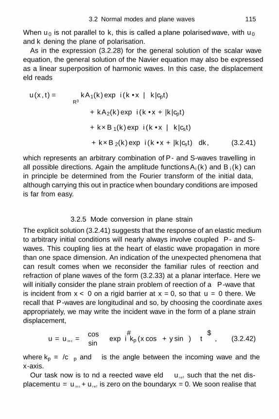
3.2 Normal modes and plane waves 115
When u0 is not parallel to k, this is called a plane polarised wave, with u0
and k defining the plane of polarisation.As in the expression (3.2.28) for the general solution of the scalar wave
equation, the general solution of the Navier equation may also be expressedas a linear superposition of harmonic waves. In this case, the displacementfield reads
u(x, t) =∫∫∫
R3kA1(k) exp
i (k · x − |k|cpt)
+ kA2(k) exp
i (k · x + |k|cpt)
+ k×B1(k) exp
i (k · x − |k|cst)
+ k×B2(k) exp
i (k · x + |k|cst)
dk, (3.2.41)
which represents an arbitrary combination of P - and S -waves travelling inall possible directions. Again the amplitude functions Ai(k) and Bi(k) canin principle be determined from the Fourier transform of the initial data,although carrying this out in practice when boundary conditions are imposedis far from easy.
3.2.5 Mode conversion in plane strain
The explicit solution (3.2.41) suggests that the response of an elastic mediumto arbitrary initial conditions will nearly always involve coupled P - and S -waves. This coupling lies at the heart of elastic wave propagation in morethan one space dimension. An indication of the unexpected phenomena thatcan result comes when we reconsider the familiar rules of reflection andrefraction of plane waves of the form (3.2.33) at a planar interface. Here wewill initially consider the plane strain problem of reflection of a P -wave thatis incident from x < 0 on a rigid barrier at x = 0, so that u = 0 there. Werecall that P -waves are longitudinal and so, by choosing the coordinate axesappropriately, we may write the incident wave in the form of a plane straindisplacement,
u = uin c =(
cos α
sinα
)exp
i[kp (x cos α + y sin α) − ωt
], (3.2.42)
where kp = ω/cp and α is the angle between the incoming wave and thex-axis.
Our task now is to find a reflected wave field ur e f such that the net dis-placement u = ui n c +ur e f is zero on the boundary x = 0. We soon realise that

116 Linear elastodynamics
P
S
α
αx
y
Rigid
boundary
β
P
Fig. 3.2 A P -wave reflecting from a rigid boundary.
this is impossible unless we allow for two reflected waves: one P -wave andone S -wave. Otherwise, there are not enough degrees of freedom to makeboth displacement components zero on x = 0. We therefore seek a reflectedwave field of the form
ur e f = rp
(− cos γ
sin γ
)exp
i[kp (−x cos γ + y sin γ) − ωt
]+ rs
(sinβ
cos β
)exp
i[ks (−x cos β + y sin β) − ωt
], (3.2.43)
where ks = ω/cs. Recall that S -waves are transverse so the amplitude isorthogonal to the wave-vector.
From the condition u = 0 on x = 0, we find that the P -wave reflectionis specular, meaning that the angle of reflection γ is equal to the angle ofincidence α. However, the S -wave reflection angle satisfies
sinβ =cs
cpsinα (3.2.44)
and, since cp > cs, it follows that β < α, as illustrated in Figure 3.2. Thereflection coefficients are given by
rp =cos(α + β)cos(α − β)
, rs = − sin(2α)cos(α − β)
. (3.2.45)
This is our first encounter with the phenomenon of mode conversion. Aboundary will usually turn a pure P -wave (or a pure S -wave) into a combi-nation of P - and S -waves. As shown in Exercise 3.6, the same happens in

3.2 Normal modes and plane waves 117
µ1, ρ1
µ2, ρ2
µ2, ρ2
x
y
h
−h“rock”
“rock”
“coal”
Fig. 3.3 A layered elastic medium.
the case of refracted waves, and the phenomenon of total internal reflectionbecomes correspondingly more complicated.
We now describe an example that illustrates how P - and S -waves caninteract in a practical situation.
3.2.6 Love waves
Let us consider the dynamic version of antiplane strain, the static case ofwhich was introduced in Section 2.3. If the displacement field takes the formu =
(0, 0, w(x, y, t)
)T, then w satisfies
µ∇2w = µ
(∂2w
∂x2 +∂2w
∂y2
)= ρ
∂2w
∂t2, (3.2.46)
which is just the familiar two-dimensional scalar wave equation (3.1.2), withwave speed cs. This is to be expected, since antiplane strain is volume-preserving, with the displacement depending only on the transverse vari-ables.
The solution strategies presented above for two-dimensional waves on amembrane are all directly applicable to the solution of (3.2.46). Here wewill illustrate them by describing Love waves, which are antiplane strainwaves guided through a particular type of layered medium. As illustratedin Figure 3.3, the geometry is that of a uniform layer of one material, withconstant thickness 2h, encased inside an infinite expanse of a second mate-rial. This set-up might model, for example, a coal seam in a rock stratum,with the displacement in the horizontal z-direction. This is in contrast with

118 Linear elastodynamics
the situation depicted in Figure 3.2 where, if we identify the rigid boundarywith a horizontal rock stratum, the displacement is in the vertical direction.For this reason, the S -waves considered in Section 3.2.5 are referred to asSV-waves, while the antiplane S -waves described by (3.2.46) are referred toas SH-waves. The density and shear modulus of the “coal” are denoted byρ1 and µ1 respectively, while those of the “rock” are labelled ρ2 and µ2.
The transverse displacement wi(x, y, t) in either medium satisfies
c2s i
(∂2wi
∂x2 +∂2wi
∂y2
)=
∂2wi
∂t2(i = 1, 2), (3.2.47)
where csi =√
µi/ρi (i = 1, 2) are the S -wave speeds. On the boundaries ofthe seam, the displacements and tractions must be continuous, as shown inSection 1.10, so that
w1 = w2, µ1∂w1
∂y= µ2
∂w2
∂y, on y = ±h. (3.2.48)
We seek travelling-wave solutions propagating in the x-direction in whichthe displacements take the form
wi = fi (y) exp
i (kx − ωt)
. (3.2.49)
Substituting (3.2.49) into (3.2.47), we find that the functions fi(y) satisfy
f ′′i +
(ω2
c2si
− k2)
fi = 0 (3.2.50)
and, hence, are either exponential or sinusoidal. We suppose that the am-plitude of the waves decays at infinity so that
f2 = A2e−y in y > h, f2 = B2ey in y < −h, (3.2.51)
where is real and positive. In such modes, the seam acts as a wave-guide,propagating waves in the x-direction without any energy radiating or “leak-ing out” to y → ±∞ as discussed in Section 3.2.3. Substitution of (3.2.51)into (3.2.50) reveals that k and ω must be such that
c2s2k
2 − ω2 = c2s2
2 > 0. (3.2.52)
In the coal seam, we try a solution
f1 = A1 cos(my) + B1 sin(my) (3.2.53)
which may be sinusoidal if m is real or exponential if m is pure imaginary.Now (3.2.50) leads to
ω2 = c2s1k
2 + c2s1m
2, (3.2.54)

3.2 Normal modes and plane waves 119
so the Love waves propagate at a speed cL given by
c2L =
ω2
k2 = c2s1
(1 +
m2
k2
). (3.2.55)
Let us first consider symmetric modes in which B1 = 0 and B2 = A2, sothe boundary conditions (3.2.48) reduce to
A2e−h = A1 cos(mh), µ2lA2e−h = µ1mA1 sin(mh). (3.2.56)
We can view this as a system of simultaneous equations for A1 and A2,whose solution is in general A1 = A2 = 0. A nonzero solution can only existif the determinant of the system is zero, and this gives us the condition
µ1m tan mh = µ2. (3.2.57)
For antisymmetric waves, with A1 = 0 and B2 = −A2, the analogous calcu-lation in Exercise 3.7 leads to
µ1m cot mh = −µ2. (3.2.58)
It remains to determine m from either of the transcendental equations(3.2.57) or (3.2.58). These are easiest to analyse in the extreme case wherethe rock is rigid so that µ2/µ1 → ∞, and we will focus on this limit hence-forth, leaving the general case to Exercise 3.7. We then see that there are twoinfinite families of solutions, with mh = (2n + 1)π/2 for symmetric wavesor mh = nπ for antisymmetric waves, where n is an integer. From (3.2.52)and (3.2.55), we deduce the inequalities
c2s1 <
(ω
k
)2< c2
s2, (3.2.59)
which show that the waves can only exist if cs1 < cs2, that is if the wavespeed in the coal is slower than that in the rock, which is typically true inpractice. The phase speed of the waves is then bounded between cs1 andcs2 and the resulting wave-fields in the rock decay exponentially as we moveaway from the seam.
For each fixed allowable value of m, (3.2.55) shows that the wave-speedcL varies with wavenumber, with long waves travelling faster than shortones. This is our first encounter with dispersive waves, and it seems to beat odds with our knowledge that S -waves are non-dispersive. However, thedispersion relations (3.2.37) were obtained only for plane P - or S -waves inan infinite medium, and (3.2.55) illustrates how the presence of boundariescan often give rise to dispersion.

120 Linear elastodynamics
ω
k
ω = cs2k
ω = cs1k
Fig. 3.4 Dispersion relation between frequency ω and wavenumber k for symmetric(solid) and antisymmetric (dotted) Love waves. The phase speed ω/k is boundedbetween cs1 and cs2 .
We see that the lowest-frequency mode is a symmetric wave withmh = π/2 and therefore
ω2 = c2s1
(π2
4h2 + k2)
. (3.2.60)
Hence, real values of k can only exist if ω exceeds a critical cut-off frequencyπcs1/2h. The existence of a cut-off frequency below which waves cannotpropagate without attenuation is a characteristic of all waveguides.
If we do not take the limit µ2/µ1 → ∞, then the dispersion relationbetween ω and k must be obtained by eliminating , m between (3.2.52),(3.2.54) and either (3.2.57) or (3.2.58), as shown in Exercise 3.7. Crucially,the values of m satisfying (3.2.57) or (3.2.58) with > 0 are all real, so theinequalities (3.2.59) continue to hold and there is still a cut-off frequency. Asshown in Figure 3.4, there is an infinite family of waves, both symmetric andantisymmetric, and, in each case, the phase speed ω/k is bounded betweencs1 and cs2.
3.2.7 Rayleigh waves
Rayleigh discovered perhaps the most famous of all elastic waves, which canpropagate close to a planar free boundary, decaying exponentially away fromthe boundary but suffering no decay at all in the direction of propagation.We can model these waves using plane strain in y < 0 below a stress-free

3.3 Dynamic stress functions 121
boundary at y = 0, where the zero-traction condition is
µ
(∂u
∂y+
∂v
∂x
)= 2µ
∂v
∂y+ λ
(∂u
∂x+
∂v
∂y
)= 0 at y = 0. (3.2.61)
Now we seek frequency-domain solutions of the form
u = (upeκp y + useκs y) expi (kx − ωt)
, (3.2.62)
where the dispersion relations (3.2.37) for P - and S -waves tell us that
κ2p = k2 − ω2
c2p
, κ2s = k2 − ω2
c2s
. (3.2.63)
We assume as usual that k and ω are real and positive, and that Re(κp) > 0and Re(κs) > 0, so that the waves propagate without attenuation in thex-direction while decaying exponentially as y → −∞. Evidently such wavescan only exist if the wavenumber k in the x-direction is greater than bothω/cs and ω/cp. The propagation speed c = ω/k must therefore satisfy
c < cs < cp, (3.2.64)
so that Rayleigh waves inevitably travel more slowly than either P -waves orS -waves.
After the rather tortuous manipulations of Exercise 3.8, we find an equa-tion for c in the form(
2 − c2
c2s
)2
= 4(
1 − c2
c2p
)1/2 (1 − c2
c2s
)1/2
. (3.2.65)
It can be shown that this leads to a sextic equation for c but that only onepositive real value for c2 exists and satisfies (3.2.64). Rayleigh waves aretherefore non-dispersive, with a constant propagation speed c.
These results led Rayleigh to suggest that, if a P - or S -wave originated atsome source, for example an earthquake, in y < 0, mode conversion wouldcause such a wave to propagate indefinitely in the x-direction near y = 0.This hypothesis is born out by seismological observation: the radius of theearth is large enough for (3.2.61) to be a good approximation and manyearthquake records reveal the arrival of a large Rayleigh wave after first theP - and then the S -waves have been detected.
3.3 Dynamic stress functions
We now describe some of the ways in which elastic wave propagation canbe reduced to the study of scalar wave equations by the use of stress func-tions. By taking the divergence and the curl of the dynamic Navier equation
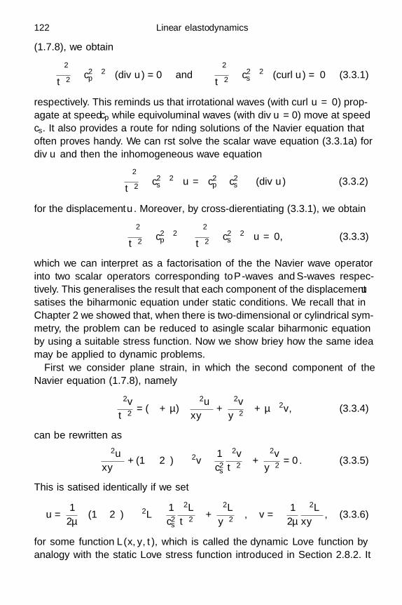
122 Linear elastodynamics
(1.7.8), we obtain(∂2
∂t2− c2
p∇2)
(div u) = 0 and(
∂2
∂t2− c2
s∇2)
(curlu) = 0 (3.3.1)
respectively. This reminds us that irrotational waves (with curlu = 0) prop-agate at speed cp while equivoluminal waves (with div u = 0) move at speedcs. It also provides a route for finding solutions of the Navier equation thatoften proves handy. We can first solve the scalar wave equation (3.3.1a) fordiv u and then the inhomogeneous wave equation(
∂2
∂t2− c2
s∇2)
u =(c2p − c2
s
)∇ (div u) (3.3.2)
for the displacement u. Moreover, by cross-differentiating (3.3.1), we obtain(∂2
∂t2− c2
p∇2)(
∂2
∂t2− c2
s∇2)
u = 0, (3.3.3)
which we can interpret as a factorisation of the the Navier wave operatorinto two scalar operators corresponding to P -waves and S -waves respec-tively. This generalises the result that each component of the displacement u
satisfies the biharmonic equation under static conditions. We recall that inChapter 2 we showed that, when there is two-dimensional or cylindrical sym-metry, the problem can be reduced to a single scalar biharmonic equationby using a suitable stress function. Now we show briefly how the same ideamay be applied to dynamic problems.
First we consider plane strain, in which the second component of theNavier equation (1.7.8), namely
ρ∂2v
∂t2= (λ + µ)
(∂2u
∂x∂y+
∂2v
∂y2
)+ µ∇2v, (3.3.4)
can be rewritten as
∂2u
∂x∂y+ (1 − 2ν)
(∇2v − 1
c2s
∂2v
∂t2
)+
∂2v
∂y2 = 0. (3.3.5)
This is satisfied identically if we set
u =12µ
(1 − 2ν)
(∇2L − 1
c2s
∂2L
∂t2
)+
∂2L
∂y2
, v = − 1
2µ
∂2L
∂x∂y, (3.3.6)
for some function L(x, y, t), which is called the dynamic Love function byanalogy with the static Love stress function introduced in Section 2.8.2. It

3.3 Dynamic stress functions 123
is then readily verified that the first Navier equation is satisfied if and onlyif L satisfies the scalar wave equation(
∂2
∂t2− c2
p∇2)(
∂2
∂t2− c2
s∇2)
L = 0. (3.3.7)
As in the static case, we could have started from the x- rather than they-component of the momentum equation, or indeed any linear combinationof the two. Thus one can define a one-parameter family of stress functionsanalogous to L.
With u and v given by (3.3.6), the stress components may be evaluatedfrom L using
τxx =∂
∂x
∂2L
∂y2 + (1 − ν)(∇2L − 1
c2s
∂2L
∂t2
), (3.3.8a)
τxy =∂
∂y
∂2L
∂y2 − ν
(∇2L − 1
c2s
∂2L
∂t2
)− 1
2c2s
∂2L
∂t2
, (3.3.8b)
τyy = − ∂
∂x
∂2L
∂y2 − ν
(∇2L − 1
c2s
∂2L
∂t2
). (3.3.8c)
For radially symmetric problems, in which the displacement takes the formu = urer + uzez and is dependent only on the cylindrical polar coordinates(r, z) and t, it is again possible to define a Love function L(r, z, t) such that
ur = − 12µ
∂2L
∂r∂z, uz =
12µ
(1 − 2ν)
(∇2L − 1
c2s
∂2L
∂t2
)+
1r
∂
∂r
(r∂L
∂r
),
(3.3.9)
and again L satisfies (3.3.7). In this case, the stress components are givenby
τrr = − ∂
∂z
∂2L
∂r2 − ν
(∇2L − 1
c2s
∂2L
∂t2
), (3.3.10a)
τrz =∂
∂r
1r
∂
∂r
(r∂L
∂r
)− ν
(∇2L − 1
c2s
∂2L
∂t2
)− 1
2c2s
∂2L
∂t2
, (3.3.10b)
τzz =∂
∂z
1r
∂
∂r
(r∂L
∂r
)+ (1 − ν)
(∇2L − 1
c2s
∂2L
∂t2
), (3.3.10c)
τθθ =∂
∂z
−1
r
∂L
∂r+ ν
(∇2L − 1
c2s
∂2L
∂t2
). (3.3.10d)
We will now use the ideas of Sections 3.2–3.3 to enumerate some of the rareconfigurations for which explicit solutions of the multidimensional elasticwave equations can be written down.
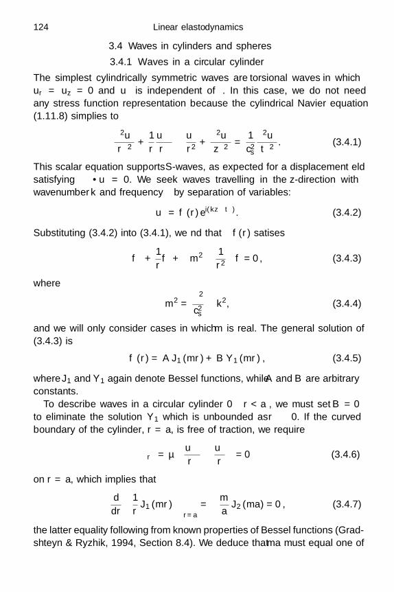
124 Linear elastodynamics
3.4 Waves in cylinders and spheres
3.4.1 Waves in a circular cylinder
The simplest cylindrically symmetric waves are torsional waves in whichur = uz = 0 and uθ is independent of θ. In this case, we do not needany stress function representation because the cylindrical Navier equation(1.11.8) simplifies to
∂2uθ
∂r2 +1r
∂uθ
∂r− uθ
r2 +∂2uθ
∂z2 =1c2s
∂2uθ
∂t2. (3.4.1)
This scalar equation supports S -waves, as expected for a displacement fieldsatisfying ∇ · u = 0. We seek waves travelling in the z-direction withwavenumber k and frequency ω by separation of variables:
uθ = f (r) ei(kz−ωt). (3.4.2)
Substituting (3.4.2) into (3.4.1), we find that f(r) satisfies
f ′′ +1rf ′ +
(m2 − 1
r2
)f = 0, (3.4.3)
where
m2 =ω2
c2s
− k2, (3.4.4)
and we will only consider cases in which m is real. The general solution of(3.4.3) is
f (r) = A J1 (mr) + B Y1 (mr) , (3.4.5)
where J1 and Y1 again denote Bessel functions, while A and B are arbitraryconstants.
To describe waves in a circular cylinder 0 r < a, we must set B = 0to eliminate the solution Y1 which is unbounded as r → 0. If the curvedboundary of the cylinder, r = a, is free of traction, we require
τrθ = µ
(∂uθ
∂r− uθ
r
)= 0 (3.4.6)
on r = a, which implies that
ddr
(1r
J1 (mr))∣∣∣∣
r=a
= −m
aJ2 (ma) = 0, (3.4.7)
the latter equality following from known properties of Bessel functions (Grad-shteyn & Ryzhik, 1994, Section 8.4). We deduce that ma must equal one of

3.4 Waves in cylinders and spheres 125
the zeros ξ2,n of J2 as defined in Section 3.2.1. There is thus one family ofwaves corresponding to each integer value of n.
The dispersion relation
ω =cs
a
√ξ22,n + k2a2 (3.4.8)
tells us that the bar acts as a wave-guide, in which the frequency must exceedthe cut-off value ξ2,1cs/a, while the phase velocity ω/k is not constant, butis bounded below by cs. Torsional waves are therefore dispersive, and alwaystravel faster than S -waves. Also, for a cylinder that is finite in the z-direction,we can use (3.4.8) to find the normal frequencies.
For cylindrically symmetric longitudinal waves, in which uθ = 0 andur and uz are independent of θ, the Love stress function L introduced inSection 3.3 is especially useful. We look for harmonic waves propagating inthe z-direction by setting
L(r, z, t) = f(r)ei(kz−ωt). (3.4.9)
The partial differential equation (3.3.7) satisfied by L leads to the ordinarydifferential equation(
d2
dr2 +1r
ddr
+ m2p
)(d2
dr2 +1r
ddr
+ m2s
)f(r) = 0, (3.4.10)
for f , where now we define
m2p =
ω2
c2p
− k2, m2s =
ω2
c2s
− k2, (3.4.11)
as shorthand.The general solution of (3.4.10) is
f(r) = A J0 (mpr) + B J0 (msr) + C Y0 (mpr) + D Y0 (msr) , (3.4.12)
where A, B, C and D are arbitrary constants. To describe waves in the solidcylinder r < a, we must choose C = D = 0 so that f(r) is well-defined asr → 0. If the boundary is stress-free, then τrr and τrz are zero on r = a, andthis leads to the two boundary conditions
ddr
(1 − ν)
(f ′′ +
f ′
r
)+(
νk2 + (2 − ν)ω2
2c2s
)f
= 0, (3.4.13a)
(1 − ν)f ′′ − νf ′
r− νm2
sf = 0 (3.4.13b)
on r = a. These give us a homogeneous linear system for the two remaining
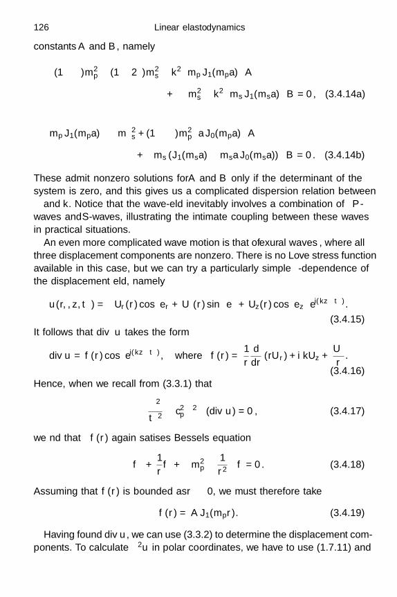
126 Linear elastodynamics
constants A and B, namely((1 − ν)m2
p − (1 − 2ν)m2s − k2)mp J1(mpa)
A
+(
m2s − k2)ms J1(msa)
B = 0, (3.4.14a)
mp J1(mpa) −
(νm2
s + (1 − ν)m2p
)a J0(mpa)
A
+
ms (J1(msa) − msa J0(msa))
B = 0. (3.4.14b)
These admit nonzero solutions for A and B only if the determinant of thesystem is zero, and this gives us a complicated dispersion relation betweenω and k. Notice that the wave-field inevitably involves a combination of P -waves and S -waves, illustrating the intimate coupling between these wavesin practical situations.
An even more complicated wave motion is that of flexural waves, where allthree displacement components are nonzero. There is no Love stress functionavailable in this case, but we can try a particularly simple θ-dependence ofthe displacement field, namely
u(r, θ, z, t) =(Ur(r) cos θer + Uθ(r) sin θeθ + Uz(r) cos θez
)ei(kz−ωt).
(3.4.15)It follows that div u takes the form
div u = f(r) cos θei(kz−ωt), where f(r) =1r
ddr
(rUr) + ikUz +Uθ
r.
(3.4.16)Hence, when we recall from (3.3.1) that(
∂2
∂t2− c2
p∇2)
(div u) = 0, (3.4.17)
we find that f(r) again satisfies Bessel’s equation
f ′′ +1rf ′ +
(m2
p −1r2
)f = 0. (3.4.18)
Assuming that f(r) is bounded as r → 0, we must therefore take
f(r) = A J1(mpr). (3.4.19)
Having found div u, we can use (3.3.2) to determine the displacement com-ponents. To calculate ∇2u in polar coordinates, we have to use (1.7.11) and
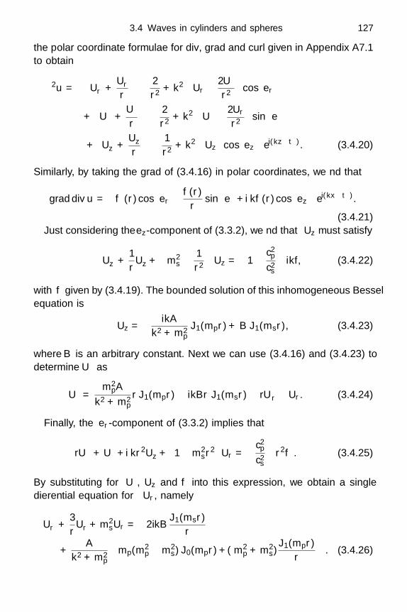
3.4 Waves in cylinders and spheres 127
the polar coordinate formulae for div, grad and curl given in Appendix A7.1to obtain
∇2u =[
U ′′r +
U ′r
r−(
2r2 + k2
)Ur −
2Uθ
r2
]cos θer
+[U ′′
θ +U ′
θ
r−(
2r2 + k2
)Uθ −
2Ur
r2
]sin θeθ
+[U ′′
z +U ′
z
r−(
1r2 + k2
)Uz
]cos θez
ei(kz−ωt). (3.4.20)
Similarly, by taking the grad of (3.4.16) in polar coordinates, we find that
grad div u =
f ′(r) cos θer −f(r)
rsin θeθ + ikf(r) cos θez
ei(kx−ωt).
(3.4.21)Just considering the ez-component of (3.3.2), we find that Uz must satisfy
U ′′z +
1rU ′
z +(
m2s −
1r2
)Uz =
(1 −
c2p
c2s
)ikf, (3.4.22)
with f given by (3.4.19). The bounded solution of this inhomogeneous Besselequation is
Uz = − ikA
k2 + m2p
J1(mpr) + B J1(msr), (3.4.23)
where B is an arbitrary constant. Next we can use (3.4.16) and (3.4.23) todetermine Uθ as
Uθ =m2
pA
k2 + m2p
r J1(mpr) − ikBr J1(msr) − rU ′r − Ur. (3.4.24)
Finally, the er-component of (3.3.2) implies that
rU ′θ + Uθ + ikr2U ′
z +(1 − m2
sr2)Ur =
(c2p
c2s
)r2f ′. (3.4.25)
By substituting for Uθ , Uz and f into this expression, we obtain a singledifferential equation for Ur , namely
U ′′r +
3rU ′
r + m2sUr = −2ikB
J1(msr)r
+A
k2 + m2p
(mp(m2
p − m2s) J0(mpr) + (m2
p + m2s)
J1(mpr)r
). (3.4.26)

128 Linear elastodynamics
z
8π/5ω6π/5ω4π/5ω2π/5ωt = 0
Fig. 3.5 Illustration of flexural waves.
Since the general bounded solution of (3.4.26) is
Ur =ikB
2ms
(J0(msr) − J2(msr)
)− mpA
2(k2 + m2p)(J0(mpr) − J2(mpr)
)+ C
J1(msr)r
, (3.4.27)
where C is a further arbitrary constant, we can finally obtain Uθ from(3.4.24) as
Uθ =A
k2 + m2p
J1(mpr)r
− ikB
m2s
J1(msr)r
+ C
(J1(msr)
r− ms J0(msr)
).
(3.4.28)Now we can look for waves in a traction-free cylinder r < a by setting
τrr = τrθ = τrz = 0 on r = a. This leads to a system of three homogeneouslinear equations for the three constants A, B and C. For nontrivial solutionsto exist, the determinant of the system must be zero as usual and thiscondition leads to the dispersion relation for flexural waves. We illustrate atypical displacement in Figure 3.5 which shows typical waves correspondingto bending, or flexing, of the cylinder propagating in the z-direction.
3.4.2 Waves in a sphere
The simplest waves in a sphere are spherically symmetric with a purelyradial displacement, that is
u = ur(r, t)er. (3.4.29)
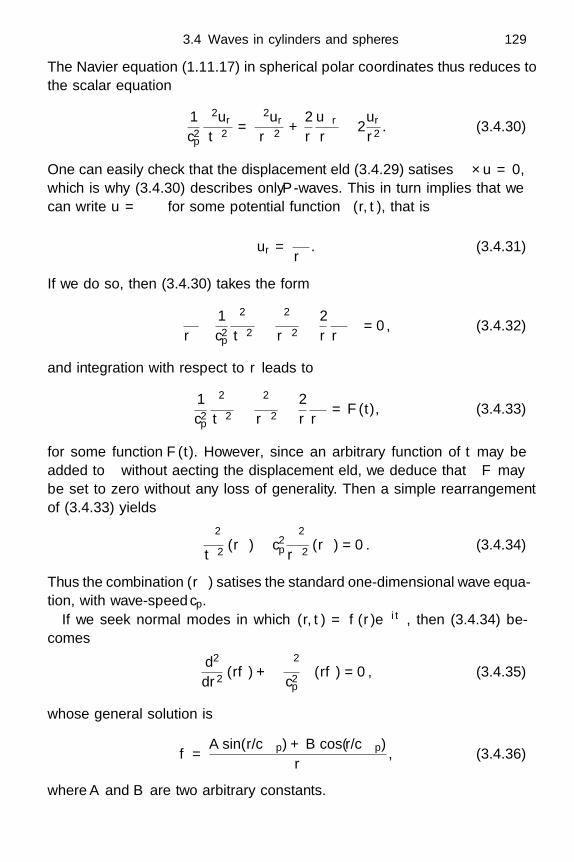
3.4 Waves in cylinders and spheres 129
The Navier equation (1.11.17) in spherical polar coordinates thus reduces tothe scalar equation
1c2p
∂2ur
∂t2=
∂2ur
∂r2 +2r
∂ur
∂r− 2
ur
r2 . (3.4.30)
One can easily check that the displacement field (3.4.29) satisfies ∇×u = 0,which is why (3.4.30) describes only P -waves. This in turn implies that wecan write u = ∇φ for some potential function φ(r, t), that is
ur =∂φ
∂r. (3.4.31)
If we do so, then (3.4.30) takes the form
∂
∂r
1c2p
∂2φ
∂t2− ∂2φ
∂r2 − 2r
∂φ
∂r
= 0, (3.4.32)
and integration with respect to r leads to
1c2p
∂2φ
∂t2− ∂2φ
∂r2 − 2r
∂φ
∂r= F (t), (3.4.33)
for some function F (t). However, since an arbitrary function of t may beadded to φ without affecting the displacement field, we deduce that F maybe set to zero without any loss of generality. Then a simple rearrangementof (3.4.33) yields
∂2
∂t2(rφ) − c2
p
∂2
∂r2 (rφ) = 0. (3.4.34)
Thus the combination (rφ) satisfies the standard one-dimensional wave equa-tion, with wave-speed cp.
If we seek normal modes in which φ(r, t) = f(r)e−iωt, then (3.4.34) be-comes
d2
dr2 (rf) +(
ω2
c2p
)(rf) = 0, (3.4.35)
whose general solution is
f =A sin(ωr/cp) + B cos(ωr/cp)
r, (3.4.36)
where A and B are two arbitrary constants.

130 Linear elastodynamics
To describe normal modes in a sphere r < a, the boundedness of φ atr = 0 implies that B = 0. If the surface r = a is traction-free, then τrr mustbe zero there. Using the formula given in Section 1.11.3, we obtain
τrr = (λ + 2µ)∂ur
∂r+ 2λ
ur
r= ρe−iωt
c2pf
′′ +2(c2
p − 2c2s)
rf ′
(3.4.37)
and, with f(r) given by (3.4.36), we find that the zero-stress condition onr = a reduces to
tan(ωa/cp)ωa/cp
=(
1 − ω2a2
4c2s
)−1
. (3.4.38)
By plotting the left- and right-hand sides versus ω, one can easily deduce thatthis transcendental equation admits a countably infinite set of real solutionsfor ω, corresponding to the natural frequencies for radial oscillations of thesphere.
More complicated formulae for solutions that are not radially symmetricmay be found in Love (1944, Chapter 12). These involve so-called sphericalharmonics, which inevitably arise when one attempts to separate the vari-ables in spherical polar coordinates. We will only discuss torsional waves, inwhich the displacement consists of just a rotation about the z-axis, so thatu = uφeφ. Using (1.11.17), one can easily show that this is only possible ifuφ is independent of φ, and it follows that div u is identically zero and wehave pure S -waves.
The Navier equation (1.11.17) reduces to
1c2s
∂2uφ
∂t2=
1r2
∂
∂r
(r2 ∂uφ
∂r
)+
1r2 sin θ
∂
∂θ
(sin θ
∂uφ
∂θ
)− uφ
r2 sin2 θ, (3.4.39)
and we seek a separable normal mode in which
uφ(r, θ, t) = f(r)g(θ)e−iωt. (3.4.40)
By separating the variables in the usual way, we find that the functions f
and g must satisfy
r2f ′′ + 2rf ′ +(
ω2r2
c2s
− κ
)f = 0, (3.4.41a)
g′′ + cot θg′ +(κ − cosec2 θ
)g = 0, (3.4.41b)
where κ is an arbitrary separation constant.Crucially, we require uφ to be a 2π-periodic function of θ and to be well-
behaved at θ = 0, π. We can now use a well-known result from quantummechanics to assert that this is possible only if κ = n(n + 1), where n is a
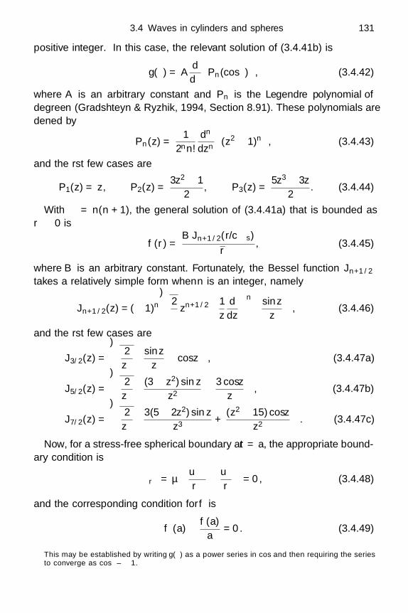
3.4 Waves in cylinders and spheres 131
positive integer.† In this case, the relevant solution of (3.4.41b) is
g(θ) = Addθ
(Pn(cos θ)
), (3.4.42)
where A is an arbitrary constant and Pn is the Legendre polynomial ofdegree n (Gradshteyn & Ryzhik, 1994, Section 8.91). These polynomials aredefined by
Pn(z) =1
2nn!dn
dzn
((z2 − 1)n
), (3.4.43)
and the first few cases are
P1(z) = z, P2(z) =3z2 − 1
2, P3(z) =
5z3 − 3z
2. (3.4.44)
With κ = n(n + 1), the general solution of (3.4.41a) that is bounded asr → 0 is
f(r) =B Jn+1/2(ωr/cs)√
r, (3.4.45)
where B is an arbitrary constant. Fortunately, the Bessel function Jn+1/2takes a relatively simple form when n is an integer, namely
Jn+1/2(z) = (−1)n
√2π
zn+1/2(
1z
ddz
)n (sin z
z
), (3.4.46)
and the first few cases are
J3/2(z) =
√2πz
(sin z
z− cos z
), (3.4.47a)
J5/2(z) =
√2πz
((3 − z2) sin z
z2 − 3 cos z
z
), (3.4.47b)
J7/2(z) =
√2πz
(3(5 − 2z2) sin z
z3 +(z2 − 15) cos z
z2
). (3.4.47c)
Now, for a stress-free spherical boundary at r = a, the appropriate bound-ary condition is
τrφ = µ
(∂uφ
∂r− uφ
r
)= 0, (3.4.48)
and the corresponding condition for f is
f ′(a) − f(a)a
= 0. (3.4.49)
†This may be established by writing g(θ) as a power series in cos θ and then requiring the seriesto converge as cos θ → ±1.
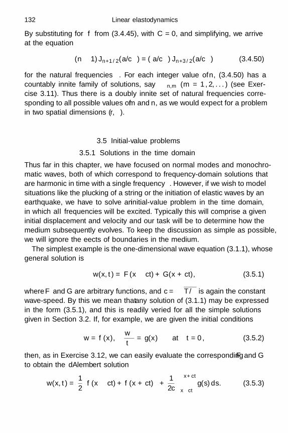
132 Linear elastodynamics
By substituting for f from (3.4.45), with C = 0, and simplifying, we arriveat the equation
(n − 1) Jn+1/2(ωa/c) = (ωa/c) Jn+3/2(ωa/c) (3.4.50)
for the natural frequencies ω. For each integer value of n, (3.4.50) has acountably infinite family of solutions, say ωn,m (m = 1, 2, . . . ) (see Exer-cise 3.11). Thus there is a doubly infinite set of natural frequencies corre-sponding to all possible values of m and n, as we would expect for a problemin two spatial dimensions (r, θ).
3.5 Initial-value problems
3.5.1 Solutions in the time domain
Thus far in this chapter, we have focused on normal modes and monochro-matic waves, both of which correspond to frequency-domain solutions thatare harmonic in time with a single frequency ω. However, if we wish to modelsituations like the plucking of a string or the initiation of elastic waves by anearthquake, we have to solve an initial-value problem in the time domain,in which all frequencies will be excited. Typically this will comprise a giveninitial displacement and velocity and our task will be to determine how themedium subsequently evolves. To keep the discussion as simple as possible,we will ignore the effects of boundaries in the medium.
The simplest example is the one-dimensional wave equation (3.1.1), whosegeneral solution is
w(x, t) = F (x − ct) + G(x + ct), (3.5.1)
where F and G are arbitrary functions, and c =√
T/ is again the constantwave-speed. By this we mean that any solution of (3.1.1) may be expressedin the form (3.5.1), and this is readily verified for all the simple solutionsgiven in Section 3.2. If, for example, we are given the initial conditions
w = f(x),∂w
∂t= g(x) at t = 0, (3.5.2)
then, as in Exercise 3.12, we can easily evaluate the corresponding F and G
to obtain the d’Alembert solution
w(x, t) =12
(f(x − ct) + f(x + ct)
)+
12c
∫ x+ct
x−ctg(s) ds. (3.5.3)
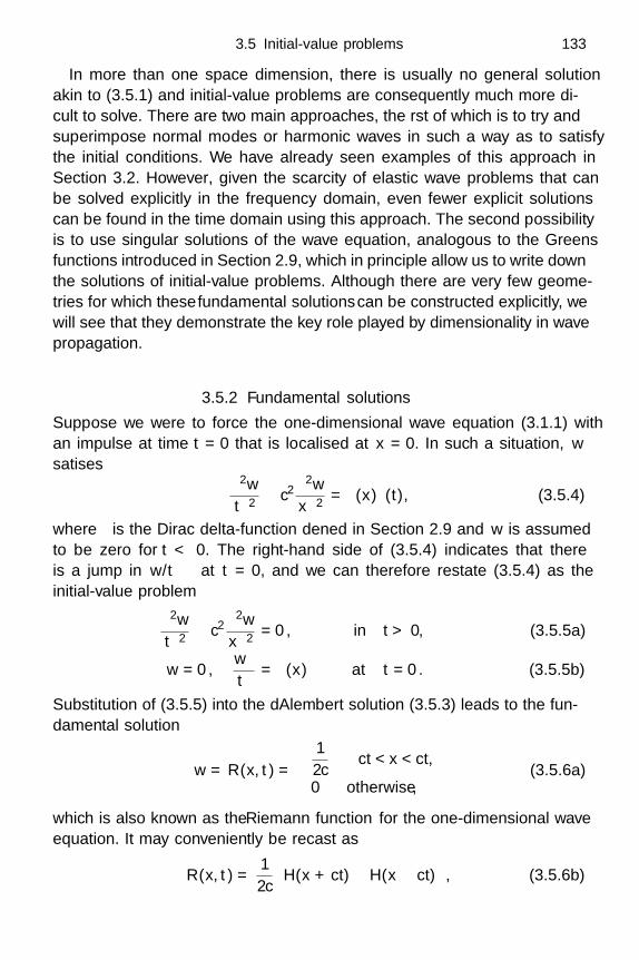
3.5 Initial-value problems 133
In more than one space dimension, there is usually no general solutionakin to (3.5.1) and initial-value problems are consequently much more diffi-cult to solve. There are two main approaches, the first of which is to try andsuperimpose normal modes or harmonic waves in such a way as to satisfythe initial conditions. We have already seen examples of this approach inSection 3.2. However, given the scarcity of elastic wave problems that canbe solved explicitly in the frequency domain, even fewer explicit solutionscan be found in the time domain using this approach. The second possibilityis to use singular solutions of the wave equation, analogous to the Green’sfunctions introduced in Section 2.9, which in principle allow us to write downthe solutions of initial-value problems. Although there are very few geome-tries for which these fundamental solutions can be constructed explicitly, wewill see that they demonstrate the key role played by dimensionality in wavepropagation.
3.5.2 Fundamental solutions
Suppose we were to force the one-dimensional wave equation (3.1.1) withan impulse at time t = 0 that is localised at x = 0. In such a situation, w
satisfies∂2w
∂t2− c2 ∂2w
∂x2 = δ(x)δ(t), (3.5.4)
where δ is the Dirac delta-function defined in Section 2.9 and w is assumedto be zero for t < 0. The right-hand side of (3.5.4) indicates that thereis a jump in ∂w/∂t at t = 0, and we can therefore restate (3.5.4) as theinitial-value problem
∂2w
∂t2− c2 ∂2w
∂x2 = 0, in t > 0, (3.5.5a)
w = 0,∂w
∂t= δ(x) at t = 0. (3.5.5b)
Substitution of (3.5.5) into the d’Alembert solution (3.5.3) leads to the fun-damental solution
w = R(x, t) =
12c
−ct < x < ct,
0 otherwise,(3.5.6a)
which is also known as the Riemann function for the one-dimensional waveequation. It may conveniently be recast as
R(x, t) =12c
(H(x + ct) − H(x − ct)
), (3.5.6b)

134 Linear elastodynamics
t
R(x, t)
x
Fig. 3.6 The one-dimensional fundamental solution R(x, t).
which is explicitly in the form of (3.5.1), where
H(s) =
0 s < 0,
1 s > 0,(3.5.7)
is the so-called Heaviside function or step function.On the other hand, if w starts from rest with the initial displacement a
localised singularity of the form
w(x, 0) = δ(x),∂w
∂t(x, 0) = 0, (3.5.8)
then we easily find that
w =12
(δ(x + ct) + δ(x − ct)
). (3.5.9)
This solution might represent the behaviour of a string that is plucked ata single point, while the fundamental solution R(x, t) models a string beingstruck at a point. Since formal differentiation† gives H ′(s) = δ(s), it followsthat w = ∂R/∂t, and we can thus write the general d’Alembert solution(3.5.3) as a superposition of fundamental solutions, namely
w(x, t) =∂
∂t
∫ ∞
∞f(s)R(x − s, t) ds +
∫ ∞
−∞g(s)R(x − s, t) ds. (3.5.10)
The Riemann function thus plays an analogous role to that performed bythe Green’s function in elastostatic problems.
We plot the fundamental solution R(x, t) in Figure 3.6. Notice that theinitial disturbance is felt everywhere inside the region |x| < ct, but nowhere
†for example noting that d(|s|)/ds = H(s) + 1 and using Exercise 2.23
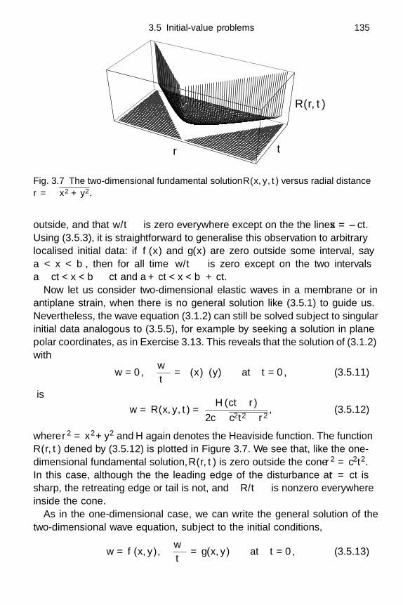
3.5 Initial-value problems 135
r t
R(r, t)
Fig. 3.7 The two-dimensional fundamental solution R(x, y, t) versus radial distancer =
√x2 + y2 .
outside, and that ∂w/∂t is zero everywhere except on the the lines x = ±ct.Using (3.5.3), it is straightforward to generalise this observation to arbitrarylocalised initial data: if f(x) and g(x) are zero outside some interval, saya < x < b, then for all time ∂w/∂t is zero except on the two intervalsa − ct < x < b − ct and a + ct < x < b + ct.
Now let us consider two-dimensional elastic waves in a membrane or inantiplane strain, when there is no general solution like (3.5.1) to guide us.Nevertheless, the wave equation (3.1.2) can still be solved subject to singularinitial data analogous to (3.5.5), for example by seeking a solution in planepolar coordinates, as in Exercise 3.13. This reveals that the solution of (3.1.2)with
w = 0,∂w
∂t= δ(x)δ(y) at t = 0, (3.5.11)
isw = R(x, y, t) =
H (ct − r)2πc
√c2t2 − r2
, (3.5.12)
where r2 = x2+y2 and H again denotes the Heaviside function. The functionR(r, t) defined by (3.5.12) is plotted in Figure 3.7. We see that, like the one-dimensional fundamental solution, R(r, t) is zero outside the cone r2 = c2t2.In this case, although the the leading edge of the disturbance at r = ct issharp, the retreating edge or “tail” is not, and ∂R/∂t is nonzero everywhereinside the cone.
As in the one-dimensional case, we can write the general solution of thetwo-dimensional wave equation, subject to the initial conditions,
w = f(x, y),∂w
∂t= g(x, y) at t = 0, (3.5.13)

136 Linear elastodynamics
as a linear superposition of fundamental solutions, namely
w(x, y, t) =∫ ∞
−∞
∫ ∞
−∞g(ξ, η)R(x − ξ, y − η, t) dξdη
+∂
∂t
∫ ∞
−∞
∫ ∞
−∞f(ξ, η)R(x − ξ, y − η, t) dξdη. (3.5.14)
From this, one can infer that the properties of R noted above also apply toarbitrary localised disturbances. If the initial data f and g are zero outsidesome region, say r < a, then for all time w is zero outside the cone r = a+ct.However, the smooth tail of R implies that the disturbance persists insidethe cone for all time.
In three dimensions, as typified by (3.4.33), the radially-symmetric waveequation takes the form
1c2
∂2w
∂t2= ∇2w =
∂2w
∂r2 +2r
∂w
∂r, (3.5.15)
where now r2 = x2 +y2 + z2, and the transformation in (3.4.34) leads to thegeneral solution
w(r, t) =F (r − ct) + G(r + ct)
r, (3.5.16)
where F and G are two arbitrary scalar functions. This illustrates that, asin one-dimensional waves, a localised radially-symmetric disturbance propa-gates outwards with a sharp leading edge and a sharp tail. Huygens’ principlestates that this happens for radially-symmetric waves in any odd number ofspace dimensions, but not the two-dimensional case considered above.
We can use the general radially-symmetric solution (3.5.16) to constructthe three-dimensional Riemann function
R(x, y, z, t) =δ(r − ct)
4πcr. (3.5.17)
This enables us to write the general solution to the three-dimensional initial-value problem in a form analogous to (3.5.14), known as the retarded poten-tial solution (Ockendon et al., 2003, p. 121). Remarkably, a retarded poten-tial solution can also be written down for the full three-dimensional Navierequation, as shown in Love (1944, Section 211). However, we emphasise thatthese solutions only apply in an infinite medium, and the presence of anyboundaries usually makes it impossible to construct a Riemann function.

3.5 Initial-value problems 137
3.5.3 Characteristics
The concept of characteristics for hyperbolic partial differential equationsgives fundamental insight into wave propagation. There are several ways ofthinking about characteristics mathematically but, for our purposes, it ismost convenient to generalise (3.5.8), (3.5.9) and base our definition on thesolution of the equations that is zero for t < t0 and driven by a localisedforcing at x = x0, t = t0. As in (3.2.28b), such a forcing will excite asuperposition of plane waves of the form u = aei(k·x−ω(k)t), where
k · x − ωt = k · x0 − ωt0. (3.5.18)
As k varies, this is a family of planes in (x, t)-space through x = x0,t = t0, and geometric intuition suggests that they will envelop a cone whosevertex is at this point (see Exercise 3.14 for an analytical explanation of thisfact). For different values of x0, t0, these cones are called the characteristiccones of the system of partial differential equations. The intersections of thecharacteristic cone through (x0, t0) with the planes t = T , T > t0 are calledthe wave-fronts of the disturbance originating at (x0, t0).
For example, for the one-dimensional wave equation (3.1.1), the planes(3.5.18) are simply x ± ct = x0 ± ct0, and they coincide with the character-istics. For higher-dimensional scalar wave equations for which
ω(k) = ±ck, (3.5.19)
we can notice that the cone
|x − x0|2 = c2(t − t0)2 (3.5.20)
has normal (k, ω) in (x, t)-space and is hence the envelope of (3.5.18) as k
varies. This is illustrated in two dimensions in Figure 3.8 and Exercise 3.14gives a derivation of this result. The wave-fronts are circles or spheres in twoor three dimensions respectively.
For the unsteady Navier equation, Section 3.2.4 shows that (3.5.19) gener-alises to
(ω2 − c2
s |k|2) (
ω2 − c2p|k|2
)= 0 and hence the characteristic surface
through x = y = z = t = 0 is a two-sheeted cone(x2 + y2 + z2 − c2
pt2) (x2 + y2 + z2 − c2
st2) = 0, (3.5.21)
as illustrated in Figure 3.9 for just two spatial dimensions. This is in starkcontrast with, for example, the three-dimensional scalar wave equation orwith electromagnetic waves in isotropic media, where Maxwell’s equations,although also vectorial, admit only one wave-speed, namely the speed oflight.
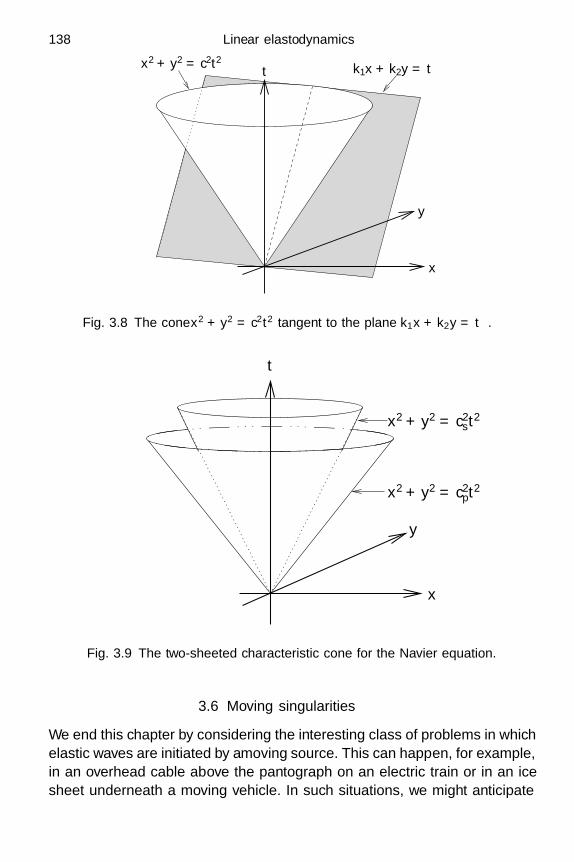
138 Linear elastodynamics
x2 + y2 = c2t2 k1x + k2y = ωt
x
y
t
Fig. 3.8 The cone x2 + y2 = c2t2 tangent to the plane k1x + k2y = ωt.
y
x
t
x2 + y2 = c2st
2
x2 + y2 = c2pt
2
Fig. 3.9 The two-sheeted characteristic cone for the Navier equation.
3.6 Moving singularities
We end this chapter by considering the interesting class of problems in whichelastic waves are initiated by a moving source. This can happen, for example,in an overhead cable above the pantograph on an electric train or in an icesheet underneath a moving vehicle. In such situations, we might anticipate

3.6 Moving singularities 139
x x
xx
w w(a) (b)
(d)(c) w w
increasing t
Fig. 3.10 The response of a string to a point force moving at speed V : (a) V = 0,(b) 0 < V < c, (c) V = c, (d) V > c.
a dramatic change in behaviour when the source velocity passes through oneof the speeds of sound in the material.
As a first illustration, consider the one-dimensional problem of an elasticstring on which a point force of magnitude P is imposed at the moving pointx = V t. This situation is modelled by the equation
∂2w
∂t2− T
∂2w
∂x2 = Pδ(x − V t), (3.6.1a)
where, as usual, δ is the Dirac delta-function. Assuming that the string startsfrom rest with zero displacement, we impose the initial conditions
w =∂w
∂t= 0 at t = 0. (3.6.1b)
This problem may be solved, for example, by changing dependent variablesto ξ = x − ct and η = x + ct, where the speed of sound is c =
√T/, to
obtain, as in Exercise 3.15,
w =Pc
4T (c2 − V 2)(c + V )|x − ct| + (c − V )|x + ct| − 2c|x − V t|
, (3.6.2)
which is a single-valued function of x when c > V .As illustrated in Figure 3.10, the gradient ∂w/∂x ahead of the force in-
creases as the propagation speed V increases, becoming infinite as V ap-proaches the speed of sound c. The assumption of small slope that under-pins the model (3.6.1a) clearly breaks down when V is close to c and, forV > c, the only continuous solution w ceases to be single-valued, as shownin Exercise 3.15 and Figure 3.10(d). In addition, we note that, no matter
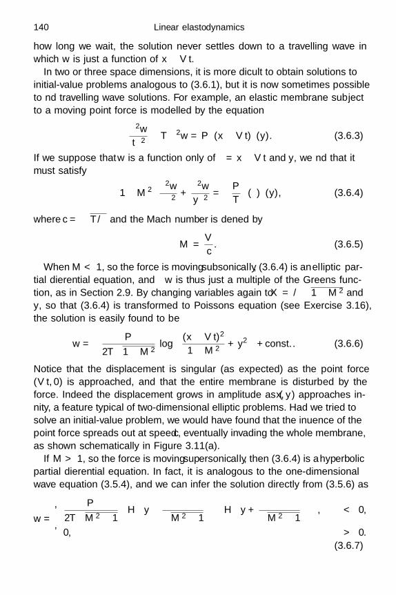
140 Linear elastodynamics
how long we wait, the solution never settles down to a travelling wave inwhich w is just a function of x − V t.
In two or three space dimensions, it is more difficult to obtain solutions toinitial-value problems analogous to (3.6.1), but it is now sometimes possibleto find travelling wave solutions. For example, an elastic membrane subjectto a moving point force is modelled by the equation
ς∂2w
∂t2− T∇2w = Pδ(x − V t)δ(y). (3.6.3)
If we suppose that w is a function only of ξ = x− V t and y, we find that itmust satisfy (
1 − M2) ∂2w
∂ξ2 +∂2w
∂y2 = −P
Tδ(ξ)δ(y), (3.6.4)
where c =√
T/ς and the Mach number is defined by
M =V
c. (3.6.5)
When M < 1, so the force is moving subsonically, (3.6.4) is an elliptic par-tial differential equation, and w is thus just a multiple of the Green’s func-tion, as in Section 2.9. By changing variables again to X = ξ/
√1 − M2 and
y, so that (3.6.4) is transformed to Poisson’s equation (see Exercise 3.16),the solution is easily found to be
w = − P
2T√
1 − M2log
((x − V t)2
1 − M2 + y2)
+ const.. (3.6.6)
Notice that the displacement is singular (as expected) as the point force(V t, 0) is approached, and that the entire membrane is disturbed by theforce. Indeed the displacement grows in amplitude as (x, y) approaches in-finity, a feature typical of two-dimensional elliptic problems. Had we tried tosolve an initial-value problem, we would have found that the influence of thepoint force spreads out at speed c, eventually invading the whole membrane,as shown schematically in Figure 3.11(a).
If M > 1, so the force is moving supersonically, then (3.6.4) is a hyperbolicpartial differential equation. In fact, it is analogous to the one-dimensionalwave equation (3.5.4), and we can infer the solution directly from (3.5.6) as
w =
P
2T√
M2 − 1
H(
y − ξ√M2 − 1
)− H
(y +
ξ√M2 − 1
), ξ < 0,
0, ξ > 0.
(3.6.7)

3.6 Moving singularities 141
y(a)
(b) y
increasing t
x
x
Fig. 3.11 Wave-fronts generated by a moving force on an elastic membrane with(a) M < 1, (b) M > 1.
Notice that we have made the “causality” assumption that w = 0 ahead ofthe point force.
In terms of physical variables, (3.6.7) may be written as
w =
P
T√
M2 − 1,
x − V t√M2 − 1
< y <V t − x√M2 − 1
,
0, otherwise,(3.6.8)
and the influence of the force is thus confined to a Mach cone, whose apexangle is tan−1
(1/√
M2 − 1)≡ sin−1(1/M). This may again be visualised
by plotting wave-fronts caused by the moving force, as in Figure 3.11(b).Since the force moves supersonically, it overtakes the wave-fronts generatedby itself. A similar wave pattern occurs behind a supersonic aircraft and isresponsible for the notorious “sonic boom”.
As was the case with (3.6.2), the subsonic (3.6.6) and supersonic (3.6.8)solutions both grow without bound as the Mach number approaches unity.This clearly violates the assumption of small displacements under which themodel (3.6.3) for an elastic membrane is valid. To describe the behaviouras M passes through unity it is therefore necessary to incorporate nonlineareffects into (3.6.3).
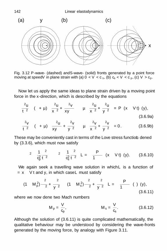
142 Linear elastodynamics
y(a) (b) (c)
x
Fig. 3.12 P -wave- (dashed) and S -wave- (solid) fronts generated by a point forcemoving at speed V in plane strain with (a) 0 < V < cs , (b) cs < V < cp , (c) V > cp .
Now let us apply the same ideas to plane strain driven by a moving pointforce in the x-direction, which is described by the equations
ρ∂2u
∂t2− (λ + µ)
(∂2u
∂x2 +∂2v
∂x∂y
)− µ
(∂2u
∂x2 +∂2u
∂y2
)= Pδ(x − V t)δ(y),
(3.6.9a)
ρ∂2v
∂t2− (λ + µ)
(∂2u
∂x∂y+
∂2v
∂y2
)− µ
(∂2v
∂x2 +∂2v
∂y2
)= 0. (3.6.9b)
These may be conveniently cast in terms of the Love stress function L definedby (3.3.6), which must now satisfy(
∇2 − 1c2p
∂2
∂t2
)(∇2 − 1
c2s
∂2
∂t2
)L = − P
1 − νδ(x − V t)δ(y). (3.6.10)
We again seek a travelling wave solution in which L is a function ofξ = x − V t and y, in which case L must satisfy(
(1 − M2p )
∂2
∂ξ2 +∂2
∂y2
)((1 − M2
s )∂2
∂ξ2 +∂2
∂y2
)L = − P
1 − νδ(ξ)δ(y),
(3.6.11)where we now define two Mach numbers
Mp =V
cp, Ms =
V
cs. (3.6.12)
Although the solution of (3.6.11) is quite complicated mathematically, thequalitative behaviour may be understood by considering the wave-frontsgenerated by the moving force, by analogy with Figure 3.11.
Exercises 143
If Mp < Ms < 1, then the motion is subsonic with respect to both P -and S -waves, and (3.6.11) is an elliptic equation similar to the biharmonicequation. In this case, as shown in Figure 3.12(a), all waves propagate outto infinity.
If Mp < 1 < Ms, then the motion is subsonic with respect to P -waves,which therefore propagate to infinity, but supersonic with respect to S -waves, which are thus confined to a Mach cone, as illustrated in Figure 3.12(b).In this transonic case, (3.6.11) is of mixed hyperbolic-elliptic type.
If Ms > Mp > 1, then the motion is entirely supersonic, so both P -wavesand S -waves are confined to Mach cones. Notice the analogy with the two-sheeted characteristic cone shown in Figure 3.9.
3.7 Concluding remarks
The ideas expounded in this chapter describe the fundamentals of manymodels that are regularly used to simulate elastic waves in situations rangingfrom tomography to oil exploration. In particular, non-destructive testing ofsolid structures is frequently carried out by examining elastic wave reflection,refraction and diffraction. In these studies, it is often the parameters λ and µ
(which will usually be functions of position) that have to be determined fromthe response of a material to elastic waves, and hence they are called inverseproblems. A classic example is the question, first posed by Kac (1966), canone hear the shape of a drum? ; in other words, if we know all the naturalfrequencies of a membrane, can we determine its boundary?†
The main complication that arises when considering the Navier equationas opposed to the scalar wave equation is the existence of two distinct wave-speeds cp and cs. Many of the problems analysed in this chapter are simpli-fied significantly if we consider incompressible materials (cf Section 1.8), inwhich cp → ∞ and div u = 0, so that A = 0 in (3.2.34) and only S -wavespropagate at finite speed.
There are many other fascinating and practically important problems inthe theory of elastic waves that fall beyond the scope of this chapter. Theseinclude finite-amplitude waves, to be discussed in Chapter 5, and wave prop-agation through inhomogeneous media, to which we will return briefly inChapter 9.
Exercises
3.1 Let a mass m be attached to a string with line density and ten-sion T . Using the boundary conditions (3.2.29) at this point, show
†The answer is now known to be no.
144 Linear elastodynamics
that the reflection and transmission coefficients for an incoming waveei(kx−ωt) are
cR =imk/2
1 − imk/2, cT =
11 − imk/2
.
3.2 Consider a wave with unit amplitude travelling in the positive x-direction on a string under tension T , whose density changes from− to + at x = 0. From continuity of the displacement and the forceat x = 0, show that this jump in density transmits a wave with am-plitude cT = 2/
(1 +
√−/+
)and reflects a wave with amplitude
cR = cT − 1.3.3 The Helmholtz equation in plane polar coordinates is
∂2A
∂r2 +1r
∂A
∂r+
1r2
∂2A
∂θ2 + k2A = 0.
To study the far field scattered from a localised obstacle, writer = R/ε, where 0 < ε 1, and use the ansatz A ∼ A0eiku(R)/ε,where A0 and u are independent of ε. Show that(
du
dR
)2
= 1, and 2∂A0
∂R+
A0
R= 0,
and deduce that outward-propagating waves take the form
A ∼ A+(θ)r−1/2eikr as r → ∞.
3.4 Show that, for any vector a and nonzero vector k, there exists aunique vector B and scalar A such that a = Ak+B×k and k·B = 0.
[Hint: calculate a · k and a×k.]3.5 Suppose that an elastic medium occupies the half-space x < 0 and
that the face x = 0 is held fixed. A plane S-wave is incident fromx → −∞ with
uinc =(
sinβ
− cos β
)expiks (x cos β + y sinβ) − iωt,
where ks = ω/cs. Show that the reflected wave takes the form
uref = rs
(sinβ
cos β
)expiks (−x cos β + y sinβ) − iωt
+rp
(− cos α
sin α
)expikp (−x cos α + y sinα) − iωt,

Exercises 145
where kp = ω/cp and the reflection angle α of the P -wave satisfies
sinα
cp=
sinβ
cs.
Show also that the reflection coefficients are given by
rs =cos(β + α)cos(β − α)
, rp =sin(2β)
cos(β − α).
What happens when β > sin−1 (cs/cp)?3.6 Suppose that the face x = 0 separates elastic media characterised by
Lame constants λ−, µ− in x < 0 and λ+, µ+ in x > 0. Derive thejump conditions[
µ
(∂u
∂y+
∂v
∂x
)]+
−=[2µ
∂u
∂x+ λ
(∂u
∂x+
∂v
∂y
)]+
−= 0
to be satisfied across x = 0. If an incident S -wave as in Exer-cise 3.5, with wave-vector (cos β−, sinβ−), generates reflected andtransmitted S - and P -waves with wave-vectors (− cos β−, sinβ−),(− cos α−, sinα−) and (cos β+, sinβ+), (cos α+, sinα+) respectively,show that
sinα−cp−
=sinβ−cs−
=sinα+
cp+=
sinβ+
cs+.
How does the number of transmitted waves vary as β− increases fromzero?
3.7 (a) Show from (3.2.52), (3.2.55) and (3.2.57) that the dispersionrelation for symmetric Love waves is given implicitly by
µ1
√ω2
c2s1
− k2 tan
(h
√ω2
c2s1
− k2
)= µ2
√k2 − ω2
c2s2
.
Write s = h√
ω2/c2s1 − k2, α = cs1/cs2, β = µ1/µ2 to obtain
the parametric representation
hω
cs2=
α√1 − α2
s√
1 + β2 tan2 s, kh =s√
α2 + β2 tan2 s√1 − α2
,
(E3.1)
where nπ s < (n + 1/2)π and n is an integer.(b) Show that antisymmetric Love waves satisfy the condition
(3.2.58) and deduce that their dispersion relation is givenparametrically by (E3.1) with tan s replaced by cot s and(n − 1/2)π s < nπ.

146 Linear elastodynamics
cg
k
cs1
cs2
Fig. 3.13 Group velocity cg = dω/dk versus wave-number k for symmetric (solid)and antisymmetric (dotted) modes of Love waves.
(c) Hence reproduce the dispersion graphs shown in Figure 3.4.(d) The group velocity cg of linear waves with dispersion relation
ω = ω(k) is defined by
cg(k) =dω
dk.
Use (E3.1) to find cg as a function of s for Love waves, andhence plot cg versus k. Deduce that, as shown in Figure 3.13,the group velocity is bounded above by cs2 but attains a localminimum before tending to cs1 as k → ∞.[This minimum in the group velocity allows an obstructionin a coal seam to be detected by studying the travel times ofreflected waves (see Tayler, 2002, Chapter 2).]
3.8 Show that up = ap(k,−iκp)T and us = as(κs,−ik)T for plane P -waves and S-waves of the form (3.2.62), where the amplitudes ap,s
are unknown. Show also that the boundary conditions (3.2.61) leadto
2kκpap + (k2 + κ2s)as = 0,(
c2p(κ
2p − k2) + 2c2
sk2) ap + 2c2
skκsas = 0,
and deduce that nonzero amplitudes exist only if the determinant
k4(c2p − 2c2
s) + k2 (2c2s(2κp − κs)κs + c2
p(κ2s − κ2
p))− c2
pκ2pκ
2s
vanishes. Using the definitions of κp,s, derive the dispersion relation(3.2.65) for Rayleigh waves. Show graphically that there is only onereal solution to this equation for the propagation speed c.

Exercises 147
3.9 In dynamic plane strain, suppose that the stress components aregiven by
τxx =∂2U
∂y2 − 12c2
s
∂2U
∂t2, τxy = − ∂2U
∂x∂y+
12c2
s
∂2φ
∂t2,
τyy =∂2U
∂x2 − 12c2
s
∂2U
∂t2,
for two functions U(x, y, t) and φ(x, y, t). Deduce from the two-dimensional Navier equation and constitutive relations that U and φ
may be chosen to satisfy(∂2
∂t2− c2
s∇2)
φ =(
∂2
∂t2− c2
p∇2)(
∂2
∂t2− c2
s∇2)
U = 0.
3.10 Show that the general solution of the scalar wave equation(∂2
∂t2− c2
p
∂2
∂x2
)(∂2
∂t2− c2
s
∂2
∂x2
)U = 0
is
U = Fp (x − cpt) + Gp (x + cpt) + Fs (x − cst) + Gs (x + cst) ,
where Fp, Gp, Fs, Gs are arbitrary scalar functions.3.11 Show that the dispersion relation (3.4.50) for torsional waves in a
sphere reduces to
tan η
η=
33 − η2 when n = 1,
tan η
η=
12 − η2
12 − 5η2 when n = 2,
tan η
η=
75 − 8η2
75 − 33η2 + η4 when n = 3,
where η = ωa/cs. By sketching the left- and right-hand sides asfunctions of η, show that there is a countably infinite set of solutionsηn,m in each case. By letting η → ∞, deduce that the highest modesare given approximately by
η1,m ∼ mπ − 3mπ
+ · · · ,
η2,m ∼ (m + 1/2)π − 5mπ
+ · · · ,
η3,m ∼ mπ − 8mπ
+ · · · ,
as m → ∞.

148 Linear elastodynamics
3.12 Show that, after a suitable change of independent variables, the one-dimensional wave equation (3.1.1) can be written as
∂2w
∂η∂ξ= 0.
Hence obtain the d’Alembert solution (3.5.1).3.13 (a) Show that the axially symmetric wave equation
1c2
∂2w
∂t2= ∇2w =
∂2w
∂r2 +1r
∂w
∂r(E3.2)
admits similarity solutions of the form
w(r, t) =1tf(r
t
),
where f(η) satisfies
ddη
(η(c2 − η2) df
dη− η2f
)= 0.
(b) Assuming that f is well-defined as η → 0, show that
f(η) =A√
c2 − η2, 0 η < c,
where A is an arbitrary constant.(c) Show that ∫ ct
0
r dr√c2t2 − r2
= ct
and deduce that
w(r, t) =
1
2πc√
c2t2 − r2, 0 r < ct,
0, r > ct,
satisfies (E3.2) subject to
w = 0,∂w
∂t= δ(x)δ(y) at t = 0.
3.14 The characteristic surface through the origin for the two-dimensionalwave equation (3.1.2) is defined to be the envelope of the planes(3.5.18) subject to the dispersion relation (3.5.19). Show that it isequivalent to the envelope of the planes
(x − x0) cos θ + (y − y0) sin θ = c(t − t0)
over all values of θ, and deduce that this is the characteristic cone(x − x0)2 + (y − y0)2 = c2(t − t0)2.
[The envelope of a one-parameter family of surfaces F (x, y, t; θ)may be found from the simultaneous equations F = ∂F/∂θ = 0.]

Exercises 149
In higher dimensions, show that
xi − x0i =cki
|k| (t − t0)
on the envelope of (3.5.18), and deduce (3.5.20).3.15 Show that, in terms of the variables ξ = x − ct and η = x + ct, the
one-dimensional wave equation (3.6.1a) subject to a moving pointsource is transformed to
∂2w
∂ξ∂η=
Pc
2T (c + V )δ
(ξ +
c − V
c + Vη
). (E3.3)
Using the fact that, from (2.9.7a),
d2
dz2
(|z|)
= 2δ(z),
deduce that the general solution of (E3.3) is
w =Pc
4T (c2 − V 2)
∣∣(c + V )ξ + (c − V )η∣∣+ F (ξ) + G(η),
where F and G are arbitrary functions. Transform back to (x, t)and apply the initial conditions to obtain the solution (3.6.2) whenc > V .
When V > c, write x − V t = X and show that (3.6.1a) becomes(V 2 − c2) ∂2w
∂X2 − 2V∂2w
∂X∂t+
∂2w
∂t2=
Pc2
Tδ(X).
Deduce that ∂w/∂X suffers a jump of Pc2/T (V 2−c2) across x = V t
and hence obtain (3.6.2).3.16 Prove the identity
δ(ax) ≡ 1|a|δ(x),
where δ is the Dirac delta-function. Hence show that, in terms ofX = ξ/
√1 − M2 and y, (3.6.4) reads
∂2w
∂X2 +∂2w
∂y2 = − P
T√
1 − M2δ(X)δ(y)
and deduce that
w = −P log
(X2 + y2
)2T
√1 − M2
+ const..
4
Approximate theories
4.1 Introduction
So far in this book we have been considering linear elasticity only for verysimple geometries such as cylinders, spheres and half-spaces. In this chapter,we will consider more general solids under the restriction that they are thinand the equations of elasticity can consequently be simplified. A familiarexample that we have already encountered is the wave equation governingthe transverse displacements of a thin elastic string, and we will revisit thismodel below in Section 4.3.
A string is characterised by its inability to withstand any appreciable shearstress, so its only internal force is a tension acting in the tangential direction.Similarly, a membrane is a thin, nearly two-dimensional structure, such asthe skin of a drum, which supports only in-plane tensions. A bar, on the otherhand, is a nearly one-dimensional solid that can be subject to either tensionor compression. However, many thin elastic bodies also have an appreciablebending stiffness and therefore admit internal shear stress as well as tension.A familiar example is a flexible ruler, which clearly resists bending whiledeforming transversely in two dimensions, and is known as a beam. A thin,nearly one-dimensional object which can bend in both transverse directions,such as a curtain rod or a strand of hair, will be referred to as a rod. Onthe other hand, a nearly planar elastic structure with significant bendingstiffness, for example a pane of glass or a stiff piece of paper, is called aplate. Finally, a shell is a thin, nearly two-dimensional elastic body which isnot initially planar, for example a ping-pong ball or the curved panel of acar.
In this chapter, we will show how models for all these structures can bederived using net force and moment balances combined with plausible con-stitutive relations. We will soon find, however, that it is difficult to enunciate
150
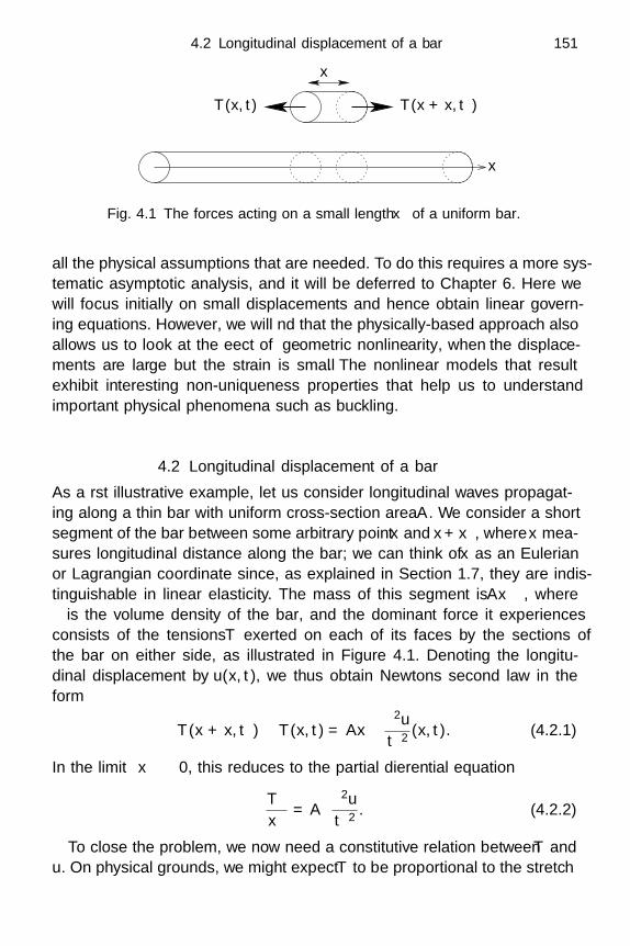
4.2 Longitudinal displacement of a bar 151
x
T (x, t) T (x + δx, t)
δx
Fig. 4.1 The forces acting on a small length δx of a uniform bar.
all the physical assumptions that are needed. To do this requires a more sys-tematic asymptotic analysis, and it will be deferred to Chapter 6. Here wewill focus initially on small displacements and hence obtain linear govern-ing equations. However, we will find that the physically-based approach alsoallows us to look at the effect of geometric nonlinearity, when the displace-ments are large but the strain is small. The nonlinear models that resultexhibit interesting non-uniqueness properties that help us to understandimportant physical phenomena such as buckling.
4.2 Longitudinal displacement of a bar
As a first illustrative example, let us consider longitudinal waves propagat-ing along a thin bar with uniform cross-section area A. We consider a shortsegment of the bar between some arbitrary point x and x+δx, where x mea-sures longitudinal distance along the bar; we can think of x as an Eulerianor Lagrangian coordinate since, as explained in Section 1.7, they are indis-tinguishable in linear elasticity. The mass of this segment is ρAδx, whereρ is the volume density of the bar, and the dominant force it experiencesconsists of the tensions T exerted on each of its faces by the sections ofthe bar on either side, as illustrated in Figure 4.1. Denoting the longitu-dinal displacement by u(x, t), we thus obtain Newton’s second law in theform
T (x + δx, t) − T (x, t) = ρAδx∂2u
∂t2(x, t). (4.2.1)
In the limit δx → 0, this reduces to the partial differential equation
∂T
∂x= ρA
∂2u
∂t2. (4.2.2)
To close the problem, we now need a constitutive relation between T andu. On physical grounds, we might expect T to be proportional to the stretch

152 Approximate theories
∂u/∂x, by analogy with Hooke’s law. Motivated by the exact static solutionobtained in Section 2.2.3, we postulate the constitutive relation
T = EA∂u
∂x, (4.2.3)
where E again denotes Young’s modulus. By substituting (4.2.3) into (4.2.2),we find that u(x, t) satisfies the wave equation
E∂2u
∂x2 = ρ∂2u
∂t2, (4.2.4)
which says that longitudinal waves in the bar travel with speed√
E/ρ.Since E < λ + 2µ, these waves travel slower than the longitudinal P-wavesof Section 3.2.4. Typical boundary conditions are that u or the axial forceEA∂u/∂x should be prescribed at each end of the bar and, of course, u and∂u/∂t need to be given at t = 0.
We should point out that various implicit assumptions underly the deriva-tion given above. We have assumed, for example, that the longitudinal dis-placement u is uniform in each cross-section of the bar, and that the con-stitutive relation (4.2.3) holds, although its derivation in Section 2.2.3 wasperformed only under static conditions. Neither of these assumptions is ex-actly true in practice, reflecting the fact that solutions of (4.2.4) are notexact solutions of the Navier equations. Intuitively, we expect (4.2.4) to bea good approximate model when the bar is thin and the displacement issmall, specifically if |u|
√A L, where L is the length of the bar. How-
ever, this simple example illustrates the difficulty of assessing the validity ofsuch an ad hoc model. We will show in Chapter 6 how such models can bederived from the underlying continuum equations in a more rigorous mannerthat allows the accuracy to be carefully estimated.
4.3 Transverse displacements of a string
Before deriving a model for the transverse displacements of a beam, let usremind ourselves briefly of the corresponding derivation for an elastic string,which is characterised by the fact that the only internal force that it cansupport is a tension T acting in the tangential direction. Assuming thatgravity g acts transversely to the string, as illustrated in Figure 4.2, the netforce experienced by a small segment of undisturbed length δx is[
T
(cos θ
sin θ
)]x+δx
x
+(
0−g
)δx,
where denotes the line density.
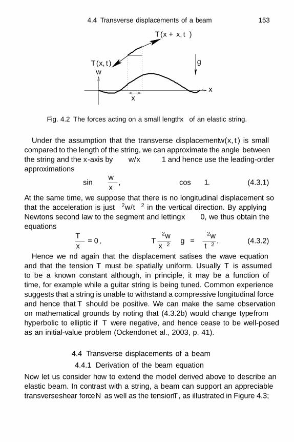
4.4 Transverse displacements of a beam 153
x
w
δx
T (x, t)
T (x + δx, t)
g
θ
Fig. 4.2 The forces acting on a small length δx of an elastic string.
Under the assumption that the transverse displacement w(x, t) is smallcompared to the length of the string, we can approximate the angle θ betweenthe string and the x-axis by θ ∼ ∂w/∂x 1 and hence use the leading-orderapproximations
sin θ ∼ ∂w
∂x, cos θ ∼ 1. (4.3.1)
At the same time, we suppose that there is no longitudinal displacement sothat the acceleration is just ∂2w/∂t2 in the vertical direction. By applyingNewton’s second law to the segment and letting δx → 0, we thus obtain theequations
∂T
∂x= 0, T
∂2w
∂x2 − g = ∂2w
∂t2. (4.3.2)
Hence we find again that the displacement satisfies the wave equationand that the tension T must be spatially uniform. Usually T is assumedto be a known constant although, in principle, it may be a function oftime, for example while a guitar string is being tuned. Common experiencesuggests that a string is unable to withstand a compressive longitudinal forceand hence that T should be positive. We can make the same observationon mathematical grounds by noting that (4.3.2b) would change type fromhyperbolic to elliptic if T were negative, and hence cease to be well-posedas an initial-value problem (Ockendon et al., 2003, p. 41).
4.4 Transverse displacements of a beam
4.4.1 Derivation of the beam equation
Now let us consider how to extend the model derived above to describe anelastic beam. In contrast with a string, a beam can support an appreciabletransverse shear force N as well as the tension T , as illustrated in Figure 4.3;
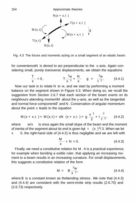
154 Approximate theories
T (x + δx, t)
T (x, t)
M(x, t)
M(x + δx, t)
g
N(x + δx, t)
N(x, t)
Fig. 4.3 The forces and moments acting on a small segment of an elastic beam.
for convenience N is defined to act perpendicular to the x-axis. Again con-sidering small, purely transverse displacements, we obtain the equations
∂T
∂x= 0, T
∂2w
∂x2 +∂N
∂x− g =
∂2w
∂t2. (4.4.1)
Now our task is to relate N to w, and we start by performing a momentbalance on the segment shown in Figure 4.3. When doing so, we recall thesuggestion from Section 2.6.7 that each section of the beam exerts on itsneighbours a bending moment M about the y-axis, as well as the tangentialand normal force components T and N . Conservation of angular momentumabout the point x leads to the equation
−M(x + δx, t) + M(x, t) + δxN(x + δx, t) = gδx2
2+ I
∂2θ
∂t2, (4.4.2)
where θ ≈ ∂w/∂x is once again the small slope of the beam and the momentof inertia of the segment about its end is given by I = (δx)3/3. When we letδx → 0, the right-hand side of (4.4.2) is thus negligible and we are left with
−∂M
∂x+ N = 0. (4.4.3)
Finally, we need a constitutive relation for M . It is a practical experience,for example when bending a flexible ruler, that applying an increasing mo-ment to a beam results in an increasing curvature. For small displacements,this suggests a constitutive relation of the form
M = −B∂2w
∂x2 , (4.4.4)
where B is a constant known as the bending stiffness. We note that (4.4.3)and (4.4.4) are consistent with the semi-infinite strip results (2.6.70) and(2.6.73) respectively.

4.4 Transverse displacements of a beam 155
x x x
(a) (b) (c)
Fig. 4.4 The end of a beam under (a) clamped, (b) simply supported and (c) freeconditions.
As in (4.2.3), we can use a simple exact solution of the Navier equationsfrom Chapter 2 to derive an equation for B. In this case we consider theplane stress solution (2.8.30) in which the displacement field and the onlynonzero stress component are
u =
u
v
w
=κ
2
−2xz
2νyz
x2 − νy2 + νz2
, τxx = −κEz. (4.4.5)
We identify the transverse displacement of the beam with κx2/2, neglectingthe small νy2 and νz2 on account of the slenderness of the beam. The netmoment generated by this stress field on the cross-section A is given by
M =∫∫
Azτxx dydz = −Eκ
∫∫A
z2 dydz, (4.4.6)
which corresponds to (4.4.4) with
B = EI, where I =∫∫
Az2 dydz (4.4.7)
is the moment of inertia of the cross-section A about the y-axis.Postulating that the constitutive relation (4.4.4) still holds under dynamic
conditions, we combine (4.4.1)–(4.4.7), to obtain the beam equation
−EI∂4w
∂x4 + T∂2w
∂x2 − g = ∂2w
∂t2. (4.4.8)
Evidently, (4.4.8) reduces to (4.3.2) as the bending stiffness EI tends to zero.Unlike the wave equation, though, (4.4.8) is not immediately classifiable aselliptic or hyperbolic.†
†It is interesting to note that the real and imaginary parts of the solution ψ of the Schrodingerequation
i∂ψ
∂t= −
2m
∂2 ψ
∂x2
satisfy (4.4.8) with T = g = 0, /2m =√
EI/.

156 Approximate theories
4.4.2 Boundary conditions
On physical grounds we expect to need to specify w and ∂w/∂t at t = 0, asfor a string. However, since (4.4.8) has four x-derivatives rather than two,we might anticipate that it requires two boundary conditions at each end ofthe beam, in contrast with a string. If, for example, a beam is clamped asshown in Figure 4.4(a), then both w and ∂w/∂x would be prescribed at theclamp; in the case illustrated
w =∂w
∂x= 0. (4.4.9)
Alternatively, we could envisage a simply supported beam end, as shown inFigure 4.4(b), where the displacement is fixed without applying any moment,so that w = M = 0 and thus
w =∂2w
∂x2 = 0. (4.4.10)
In the final example shown in Figure 4.4(c), the end of the beam is free. Ittherefore experiences no shear force or bending moment, and from (4.4.3)and (4.4.4) we deduce the boundary conditions
∂2w
∂x2 =∂3w
∂x3 = 0, (4.4.11)
and in this case we must also have T ≡ 0.If we specify distributed tractions on the end of a beam, then the only
information about them required for our model is the net force and momentthat they exert. Specifically, if the longitudinal and tangential stress com-ponents applied to the section x = 0 are σx(y, z) and σz(y, z) respectively,then the boundary conditions to be imposed on the beam equation are
T =∫∫
Aσx(y, z) dydz, N =
∫∫A
σz(y, z) dydz,
M =∫∫
Azσx(y, z) dydz. (4.4.12)
Here we are effectively invoking Saint-Venant’s principle: all details of theedge tractions apart from the three numbers T , N and M are lost out-side a neighbourhood of the edge where they are applied. We showed inSection 2.6.7 that this is true in plane strain, and here we assume that itapplies more generally.
4.4.3 Compression of a beam
One of the most dramatic new features of (4.4.8) compared with (4.3.2)is that we can now consider situations in which T < 0. We illustrate an

4.4 Transverse displacements of a beam 157
0.2 0.4 0.6 0.8 1
-1
-0.5
0.5
1
0.2 0.4 0.6 0.8 1
-1
-0.5
0.5
1
0.2 0.4 0.6 0.8 1
-1
-0.5
0.5
1
n = 1 n = 2 n = 3w w
xxx
w
Fig. 4.5 The first three buckling modes of a clamped elastic beam (with a = 1 andL = 1).
unexpected new possibility that arises in such cases by considering steadydisplacements of a beam of length L subject to negligible gravity. We supposethat the ends are clamped and subject to a compressive force P = −T andzero transverse force. In this case (4.4.8) reduces to the ordinary differentialequation
EId4w
dx4 + Pd2w
dx2 = 0, (4.4.13a)
subject to the boundary conditions
dw
dx=
d3w
dx3 = 0 at x = 0, L. (4.4.13b)
We can consider (4.4.13) as an eigenvalue problem. One possibility is alwaysthat the beam remains straight with w ≡ const. but, if the applied forcetakes one of the discrete values
P
EI=
n2π2
L2 , (4.4.14)
where n is an integer, then (4.4.13) admits the eigenfunction solution
w = A cos(nπx
L
), (4.4.15)
where A is a constant.The first three such eigenfunctions are shown in Figure 4.5; these are
the shapes that a beam can adopt as it buckles under a sufficiently largecompressive force. The amplitude A appears to be indeterminate, althoughwe might expect it to be a smoothly increasing function of the applied force.This is a deficiency of the model that will be addressed in Section 4.9.
158 Approximate theories
4.4.4 Waves on a beam
Concerning the dynamic equation (4.4.8) with g = 0 and adopting the phi-losophy of Section 3.2.2, we can seek travelling-wave solutions of the form
u = A exp(i(kx − ωt)
), (4.4.16)
where the real part is assumed as usual, and hence obtain the dispersionrelation
ω2 = EIk4 + Tk2. (4.4.17)
Elastic waves on a beam are therefore dispersive, unlike P -waves, S -waves orwaves on a string. This should not come as too much of a surprise, since wehave already discovered in Chapter 3 that elastic waves are usually dispersivein bounded domains.
For a beam under positive tension T > 0, waves with frequency ω canthus propagate with wave-length 2π/k provided
ω
k=
√T
(1 +
EIk2
T
)1/2
. (4.4.18)
Evidently this reduces to the dispersion relation for a string if the waves arelong, with k
√T/EI. However, the bending stiffness becomes increasingly
important, and the waves become increasingly dispersive, as the wave-lengthdecreases. This observation can be used to explain, for example, why theharmonics of a piano string with small but nonzero bending stiffness areslightly sharp compared with the fundamental (see Exercise 4.1).
For a beam under compression, with P = −T > 0, wave-like solutions of(4.4.8) exist only if k2 > P/EI. For smaller values of k, (4.4.17) leads tocomplex values of ω, corresponding to solutions that grow exponentially intime. It follows that the beam is unstable to waves with wave-length greaterthan 2π
√EI/P , and we will investigate this further in Section 4.9.3.
4.5 Linear rod theory
We next consider the motion of a nearly straight uniform elastic rod that canbend in two transverse directions, so that the displacement isw(x, t) =
(v(x, t), w(x, t)
)T. Now, in addition to the tension T , there aretwo shear force components Ny and Nz in the y- and z-directions respec-tively, as illustrated in Figure 4.6. By applying Newton’s second law andassuming small displacements as above, we again find that T is spatially

4.5 Linear rod theory 159
NzNy
T
yz
x
Fig. 4.6 The internal force components T , Ny and Nz in a thin elastic rod.
y
x
z
Mz
My
Mx
Fig. 4.7 Cross-section through a rod showing the bending moment components.
uniform and obtain the following generalisation of (4.4.8):
T∂2w
∂x2 +∂N
∂x+ f =
∂2w
∂t2, (4.5.1)
where N =(Ny, Nz
)T and f is the body force per unit length.In general we must now allow for three components of the bending moment
M = (Mx, My, Mz)T. As shown in Figure 4.7, My is the moment about they-axis previously referred to simply as M in Section 4.4, while Mz representsbending in the (x, y)-plane. We will begin by neglecting the first componentMx, which corresponds to twisting of the rod about its axis. A balance ofmoments in the y- and z-directions analogous to (4.4.3) then leads to
∂My
∂x− Nz = 0,
∂Mz
∂x+ Ny = 0. (4.5.2)
Finally, we need to generalise the constitutive relation (4.4.4), and we willagain use the plane stress solution (4.4.5) as a guide. By combining (4.4.5)with an analogous expression representing bending in the y-direction, we
160 Approximate theories
obtain the following exact solution of the Navier equations:
u =κz
2
−2xz
2νyz
x2 − νy2 + νz2
+κy
2
−2xy
x2 + νy2 − νz2
2νyz
, (4.5.3a)
τxx = −κzEz − κyEy. (4.5.3b)
The two constants κy and κz represent bending in the (x, y)-plane and the(x, z)-plane respectively. The moments about the y- and z-axes generatedover the cross-section A by this stress field are given by
My =∫∫
Azτxx dydz, Mz = −
∫∫A
yτxx dydz. (4.5.4)
By substituting (4.5.3) into (4.5.4) we obtain the relations(Mz
−My
)= EI
∂2w
∂x2 , (4.5.5)
where the “inertia tensor”
I =(
Iyy Iyz
Iyz Izz
)=∫∫
A
(y2 yz
yz z2
)dydz (4.5.6)
characterises the bending stiffness in each direction.Hence the generalisation of (4.4.8) is the coupled system
T∂2w
∂x2 − EI∂4w
∂x4 + f = ∂2w
∂t2. (4.5.7)
Note that we can choose the y- and z-axes such that the symmetric positivedefinite matrix I is diagonal; these correspond to the directions in which theresistance to bending is maximised and minimised. It follows that the y- andz-components of (4.5.7) are simply two decoupled beam equations for v andw; note, though, that this decoupling does not occur if the rod cross-sectionis non-uniform in x. By analogy with (4.4.8), we therefore expect to have toimpose initial conditions on w and ∂w/∂t as well as two boundary conditionseach on v and w at either end of the rod. The conditions correspondingto clamped, simply supported and free ends are obvious generalisations of(4.4.9), (4.4.10) and (4.4.11).
Examples of values of Iyy and Izz for various cross-section shapes withrespect to principal axes are given in Figure 4.8. These are crucial piecesof information to bear in mind when designing beams or rods in practice.By considering (4.5.4), we observe that Iyy measures resistance to bendingabout the z-axis, while Izz represents resistance to bending about the y-axis.For example, if one considers the bending of a long strip of paper with

4.5 Linear rod theory 161
a
b
b
(b)
(a)
(c)
Izz = a3b/12
Iyy = ab3/12
Iyy = Izz = πab(a2 + 4b2)/4Izz
Iyy < Izz
a
Fig. 4.8 Examples of cross-sections in the (y, z)-plane and their bending stiffnesses.
transverse dimensions a and b in the z- and y-directions respectively, whereb a, it is then easy to see as in Figure 4.8(a) that Izz Iyy . This explainswhy it is so much easier to bend such a strip about the y-axis than about thez-axis. On the other hand, if we roll the same paper strip into a long cylinder,it will become become much stiffer in all bending directions as illustrated inFigure 4.8(b). This situation can be seen as a limiting case of a cylindricalshell, and it gives us a hint as to why curved shells are generally much stifferthan flat rods or plates. Meanwhile, the “I-beam” in Figure 4.8(c) stronglyresists bending about the y-axis.
Proceeding along the same lines as for longitudinal waves, we now con-sider torsion, i.e. twisting a rod about its longitudinal axis. As illustrated inFigure 4.7, we denote by Mx the moment about the x-axis exerted on eachcross-section through the rod. By balancing the net torque with the rateof change of angular momentum of a small segment of length δx and thenletting δx tend to zero, we obtain
∂Mx
∂x= (Iyy + Izz)
∂2θ
∂t2, (4.5.8)
where θ(x, t) denotes the angle of twist about the x-axis.Now we refer to the exact steady solution of Section 2.4 to motivate the
constitutive relation
Mx = R∂θ
∂x(4.5.9)

162 Approximate theories
between the torque and the twisting gradient, where R again denotes thetorsional rigidity.† We thus find that θ satisfies the wave equation, with wavespeed
√R/ρ (Iyy + Izz). For the simple case of a circular cross-section, it is
easy to show that
Iyy + Izz =πa4
2, R =
πa4µ
2(4.5.10)
and hence that the wave speed is equal to cs. This reproduces the wave speedof the first family of torsional waves found in Section 3.4.1; that is, (3.4.8)with n = 0 and ξ2,0 = 0: the theory presented here assumes each sectiondeforms uniformly and thus fails to discern the higher modes.
4.6 Linear plate theory
4.6.1 Derivation of the plate equation
Now we derive the equation governing the small transverse displacementw(x, y, t) of an elastic plate that is bent out of the plane z = 0. We describethe in-plane forces using a two-dimensional stress tensor
T =(
Txx Txy
Tyx Tyy
), (4.6.1)
where Tij is the i-component of the force per unit length on a section of theplate with outward normal in the j-direction. We also denote the transverseshear force on a section with normal in the j-direction by Nj . The forcesacting on a small rectangular section of the plate are illustrated in Figure 4.9.By balancing moments around the z-axis, as in Section 1.5, we discover thatTyx ≡ Txy , so that T is symmetric. If we assume that there is no accelerationin the x- and y-directions and that the only body force is gravity acting inthe negative z-direction, then Newton’s second law gives
∂Txx
∂x+
∂Txy
∂y= 0,
∂Txy
∂x+
∂Tyy
∂y= 0 (4.6.2)
and
∂
∂x
(Nx + Txx
∂w
∂x+ Txy
∂w
∂y
)+
∂
∂y
(Ny + Txy
∂w
∂x+ Tyy
∂w
∂y
)− ςg = ς
∂2w
∂t2, (4.6.3)
where ς is now the mass of the plate per unit area.†
For consistency with the notation of this chapter, x should be substituted for z in the resultsof Section 2.4.

4.6 Linear plate theory 163
z
y
x Tyy
Tyx
Txx
Tyx
Nx
Txy
Tyy
Ny
Txx
Nx
Txy
Ny
δx
δy
Fig. 4.9 The forces acting on a small section of an elastic plate.
Considering the bending moments, we use an analogous notation Mij
(i, j = x, y) to denote the i-component of the moment per unit length actingon a section with outward normal in the j-direction, as illustrated schemati-cally in Figure 4.10. We note that Mij is not in general symmetric, althoughit is a two-dimensional tensor, as will shortly become apparent. By balancingmoments on the segment shown in Figure 4.10, we obtain the relations
∂Mxx
∂x+
∂Mxy
∂y+ Ny = 0,
∂Myx
∂x+
∂Myy
∂y− Nx = 0. (4.6.4)
Next we seek constitutive equations for the bending moments which, byanalogy with Section 4.4, we expect to be linear functions of the secondderivatives of w. Again we can use exact plane stress solutions to evaluatethe appropriate coefficients. In this case, by choosing χ0 = φ = 0 and χ1
a suitable quadratic function of x and y in (2.8.28), we can construct asolution with displacement field
u =12
−2(ax + by)z−2(bx + cy)z
ax2 + 2bxy + cy2 + ν(a + c)z2/(1 − ν)
(4.6.5)
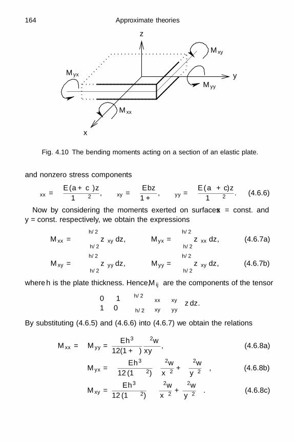
164 Approximate theories
Myy
z
x
Myx
Mxx
Mxy
y
Fig. 4.10 The bending moments acting on a section of an elastic plate.
and nonzero stress components
τxx = −E(a + νc)z1 − ν2 , τxy = − Ebz
1 + ν, τyy = −E(νa + c)z
1 − ν2 . (4.6.6)
Now by considering the moments exerted on surfaces x = const. andy = const. respectively, we obtain the expressions
Mxx = −∫ h/2
−h/2zτxy dz, Myx =
∫ h/2
−h/2zτxx dz, (4.6.7a)
Mxy = −∫ h/2
−h/2zτyy dz, Myy =
∫ h/2
−h/2zτxy dz, (4.6.7b)
where h is the plate thickness. Hence, Mij are the components of the tensor(0 −11 0
)∫ h/2
−h/2
(τxx τxy
τxy τyy
)z dz.
By substituting (4.6.5) and (4.6.6) into (4.6.7) we obtain the relations
Mxx = −Myy =Eh3
12(1 + ν)∂2w
∂x∂y, (4.6.8a)
Myx = − Eh3
12 (1 − ν2)
(∂2w
∂x2 + ν∂2w
∂y2
), (4.6.8b)
Mxy =Eh3
12 (1 − ν2)
(ν
∂2w
∂x2 +∂2w
∂y2
). (4.6.8c)

4.6 Linear plate theory 165
It is reassuring that, in the notation of this section, the plane strain result(2.6.73) implies that
Myx = − µh3
6(1 − ν)∂2w
∂x2 , (4.6.9)
which is consistent with (4.6.8b) when w = w(x). On the other hand, if wewere to bend a plate about the y-axis while applying no moment about thex-axis, then we would have Mxy = 0 and therefore
∂2w
∂y2 = −ν∂2w
∂x2 . (4.6.10)
Thus, without the imposition of a transverse bending moment, the plate willautomatically bend upwards in the y-direction when we attempt to bend itdownwards in the x-direction. Unfortunately, it is difficult to observe thiseffect using a piece of paper because Poisson’s ratio is close to zero. Bysubstituting (4.6.10) into (4.6.8b), we find in this case that
Myx =Eh3
12∂2w
∂x2 , (4.6.11)
which is consistent with (4.4.4) and (4.4.7), since h3/12 is the moment ofinertia per unit length in the y-direction. Hence we see that the constant ofproportionality between curvature and bending moment in one dimensiondepends on whether the transverse curvature or the transverse moment areset to zero. This is analogous to the biaxial strain examples considered inSection 2.2.4, where the effective one-dimensional elastic modulus dependson whether zero stress or zero strain is imposed in the transverse direction.
When we use the constitutive relations (4.6.8) in (4.6.3), we are left withthe plate equation
Txx∂2w
∂x2 + 2Txy∂2w
∂x∂y+ Tyy
∂2w
∂y2 − D∇4w − ςg = ς∂2w
∂t2, (4.6.12)
where ∇2 = ∂2/∂x2 + ∂2/∂y2 and
D =Eh3
12 (1 − ν2)(4.6.13)
is the bending stiffness of the plate. A membrane is a plate with negligiblebending stiffness, and is described by (4.6.12) with D = 0.
Unfortunately, the problem is still under-determined since (4.6.2) gives usonly two equations in the three stress components. To close the problem, wealso need constitutive relations for Txx, Txy and Tyy in terms of the in-planedisplacements of the plate. We leave this calculation to Section 4.6.5, here
166 Approximate theories
concentrating on the simple case where the plate is subjected to a knownisotropic tension T . This corresponds to the trivial exact solution of (4.6.2)in which Txx = Tyy = T and Txy = 0, and reduces (4.6.12) to
T∇2w − D∇4w − ςg = ς∂2w
∂t2. (4.6.14)
Comparison with (4.4.8) reveals the difference in bending stiffness betweena beam undergoing planar displacements and a plate deforming in two di-mensions.
4.6.2 Boundary conditions
As initial conditions for (4.6.14), we should specify w and ∂w/∂t. For aclamped plate, the boundary conditions are analogous to those for a beam,namely
w =∂w
∂n= 0, (4.6.15)
where ∂/∂n is the normal derivative.For a simply supported plate, we require the displacement and the bending
moment about an axis tangential to the boundary to be zero. The latter maybe written in the form
Msn =(−ny, nx)
(Mxx Mxy
Myx Myy
)(nx
ny
)= 0, (4.6.16)
where n = (nx, ny)T is the outward-pointing unit normal to the boundary.
By substituting for the moments from (4.6.8) and using the fact that w iszero on the boundary, we can reduce (4.6.16) to
w =∂2w
∂n2 + νκ∂w
∂n= 0, (4.6.17)
where κ is the curvature of the boundary (see Exercise 4.8). Only for astraight boundary, then, can we apply the obvious generalisation of (4.4.10)in which w and its second normal derivative are zero.
Finally we consider the boundary conditions to be imposed at a free edge,where a horizontal force balance evidently requires that T = 0. If, for thesake of argument, the boundary is at x = 0, then, for there to be zero ap-plied stress, we are apparently led to the conditions Nx = Mxx = Myx = 0.However, it is to impossible to impose three boundary conditions on thebiharmonic problem (4.6.14)! This conceptual difficulty caused great con-sternation to the pioneers of plate theory (see Love, 1944, Article 297), and
4.6 Linear plate theory 167
a version of Saint-Venant’s principle is commonly invoked to reduce thenumber of boundary conditions to two. However, a systematic resolution ofthe difficulty requires us to acknowledge that there is a narrow region nearthe free edge where the assumptions that gave rise to the plate equation fail.The careful analysis of this layer carried out in Section 6.4 shows that thecorrect conditions at a free edge x = 0 are
Myx = 0,∂Myx
∂x− 2
∂Mxx
∂y= 0 (4.6.18)
or, in terms of the displacement,
∂2w
∂x2 + ν∂2w
∂y2 = 0,∂3w
∂x3 + (2 − ν)∂3w
∂x∂y2 = 0. (4.6.19)
By using (4.6.4) and (4.6.8), we may also rewrite the second of (4.6.18) as
Nx =∂Mxx
∂y, (4.6.20)
which shows that the shear stress Nx as calculated from plate theory doesnot in general vanish at a free edge! Note also that a discontinuity in thebending moment at a corner in the boundary results in a delta-function inthe shear stress, corresponding to a point force in the transverse direction(see Timoshenko & Woinowsky-Krieger, 1959). This suggests the existenceof a three-dimensional “Saint-Venant” region in the vicinity of the corner.
It is also possible to obtain (4.6.18) as the natural boundary conditionsassociated with minimising the strain energy in the plate. Although it isbeyond the scope of this chapter to derive this systematically, we note that,in the exact solution (4.6.5) where tension is neglected, the nonzero stresscomponents are given by (4.6.6) and the corresponding strain componentsby
exx = −az, exy = −bz, eyy = −cz. (4.6.21)
Recalling the definition (1.9.5) of the strain energy density W, we find thatthe stored energy per unit plate area is∫ h/2
−h/2W dz =
∫ h/2
−h/2
12τijεij dz
=D
2a2 + 2νac + c2 + 2(1 − ν)b2
=D
2(a + c)2 + 2(1 − ν)
(b2 − ac
). (4.6.22)

168 Approximate theories
This suggests that, more generally, the net strain energy due to bending willtake the form
U =D
2
∫∫Ω
(∇2w
)2 − 2(1 − ν)
(∂2w
∂x2∂2w
∂y2 −(
∂2w
∂x∂y
)2)
dxdy,
(4.6.23)where the integral is taken over the region Ω in the (x, y)-plane occupied bythe plate. The integrand in (4.6.23) shows that the total energy depends ona combination of the mean curvature
∇2w = κ1 + κ2 (4.6.24)
and the Gaussian curvature
∂2w
∂x2∂2w
∂y2 −(
∂2w
∂x∂y
)2
= κ1κ2, (4.6.25)
where κ1 and κ2 are the principal curvatures of the surface z = w(x, y).We will soon discover that these geometric quantities are fundamental to alltheories of plates and shells.
Exercise 4.10 demonstrates that, if we minimise (4.6.23) using the calculusof variations, then w must satisfy the biharmonic equation, which agreeswith the steady version of (4.6.14), when tension and gravity are neglected.In addition, Exercise 4.10 shows that (4.6.19) are the natural boundaryconditions for the minimisation.
4.6.3 Simple solutions of the plate equation
Let us start by considering steady solutions of (4.6.14) with T = 0, that is
∇4w = − ςg
D. (4.6.26)
Solutions of (4.6.26) describe the sagging of a plate under gravity. We willconsider both clamped and simply supported boundary conditions; it is im-possible to solve (4.6.26) with entirely free boundaries since some boundarytractions are needed to balance gravity.
For example, to describe the sagging of an elastic disc r < a, we caneasily solve (4.6.26) in cylindrical polar coordinates. With clamped boundaryconditions w = dw/dr = 0 at r = a, we find that
w = − ςg
64D
(a2 − r2)2 . (4.6.27)
Alternatively, the simply supported boundary conditions (4.6.17) at r = a
lead to the solution
w = − ςg
64D
(a2 − r2)(5 + ν
1 + νa2 − r2
). (4.6.28)
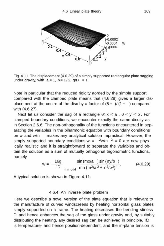
4.6 Linear plate theory 169
00.2
0.40.6
0.8
100.10.20.30.40.5-0.0006-0.0004-0.00020
00.2
0.40.6
0.8
-- w
yx
Fig. 4.11 The displacement (4.6.29) of a simply supported rectangular plate saggingunder gravity, with a = 1, b = 1/2, ςg/D = 1.
Note in particular that the reduced rigidity afforded by the simple supportcompared with the clamped plate means that (4.6.28) gives a larger dis-placement at the centre of the disc by a factor of (5 + ν)/(1 + ν) comparedwith (4.6.27).
Next let us consider the sag of a rectangle 0 < x < a, 0 < y < b. Forclamped boundary conditions, we encounter exactly the same difficulty asin Section 2.6.6. The non-orthogonality of the functions encountered in sep-arating the variables in the biharmonic equation with boundary conditionson w and ∂w/∂n makes any analytical solution impractical. However, thesimply supported boundary conditions w = ∂2w/∂n2 = 0 are now phys-ically realistic and it is straightforward to separate the variables and ob-tain the solution as a sum of mutually orthogonal trigonometric functions,namely
w =−16ςg
π6D
∑m,n odd
sin (mπx/a) sin (nπy/b)mn (m2/a2 + n2/b2)2 . (4.6.29)
A typical solution is shown in Figure 4.11.
4.6.4 An inverse plate problem
Here we describe a novel version of the plate equation that is relevant tothe manufacture of curved windscreens by heating horizontal glass platessimply supported on a frame. The heating decreases the bending stiffnessD and hence enhances the sag of the glass under gravity and, by suitablydistributing the heating, any desired sag can be achieved in principle. If D
is temperature- and hence position-dependent, and the in-plane tension is

170 Approximate theories
negligible, then the displacement satisfies
∂2
∂x2
(D
(∂2w
∂x2 + ν∂2w
∂y2
))+ 2(1 − ν)
∂2
∂x∂y
(D
∂2w
∂x∂y
)+
∂2
∂y2
(D
(∂2w
∂y2 + ν∂2w
∂x2
))+ ςg = 0. (4.6.30)
Given D(x, y), (4.6.30) is a simple generalisation of the biharmonic equationwhich is straightforward in principle to solve for w(x, y), at least numerically.The corresponding inverse problem is, given a desired sag profile w(x, y), todetermine the required distribution of the bending stiffness D(x, y). Whenviewed as a problem for D, (4.6.30) is a second-order linear partial differen-tial equation, and two immediate questions arise: “what boundary conditionsshould be imposed?” and “will D be positive?”.
Since the terms involving the highest derivatives of D in (4.6.30) are(∂2w
∂x2 + ν∂2w
∂y2
)∂2D
∂x2 + 2(1 − ν)∂2w
∂x∂y
∂2D
∂x∂y+(
∂2w
∂y2 + ν∂2w
∂x2
)∂2D
∂y2 ,
we can read off the discriminant
∆ = (1 − ν)2(
∂2w
∂x∂y
)2
−(
∂2w
∂x2 + ν∂2w
∂y2
)(∂2w
∂y2 + ν∂2w
∂x2
), (4.6.31a)
and simple rearrangements of the right-hand side yield
∆ =M2
xx + MxyMyx
D2 (4.6.31b)
= −(1 − ν)2
(∂2w
∂x2∂2w
∂y2 −(
∂2w
∂x∂y
)2)
− ν
(∂2w
∂x2 +∂2w
∂y2
)2
. (4.6.31c)
Now, if there is a simply supported edge at x = 0, then we must haveMyx = 0 there and we deduce from (4.6.31b) that ∆ > 0 and (4.6.30) istherefore hyperbolic. On the other hand, the right-hand side of (4.6.31c)shows that ∆ < 0 wherever the Gaussian curvature is positive, which we ex-pect to be the case nearly everywhere in a typical windscreen. It follows that(4.6.30) must change type somewhere between the simply supported bound-ary and the interior, and it is an interesting open question as to whethersmooth solutions to this mixed type partial differential equation exist (seeSalazar & Westbrook, 2004).
4.6.5 More general in-plane stresses
If we do not make the simplifying assumption that the in-plane stress isisotropic and known, then we need to obtain constitutive relations for the

4.6 Linear plate theory 171
components Txx, Txy and Tyy . We appeal to the exact biaxial strain solution(2.2.19) to pose the constitutive relations
Txx =Eh
1 − ν2 (exx + νeyy) , (4.6.32a)
Txy = Tyx =Eh
1 + νexy, (4.6.32b)
Tyy =Eh
1 − ν2 (νexx + eyy) , (4.6.32c)
where the linearised strain components are related to in-plane displacementsby
exx =∂u
∂x, exy =
12
(∂u
∂y+
∂v
∂x
), eyy =
∂v
∂y. (4.6.33)
We therefore have a plane strain problem to solve for the two-dimensionaldisplacement field (u, v)T.
From (4.6.2) we infer the existence of an Airy stress function A such that
Txx =∂2A
∂y2 , Txy = − ∂2A
∂x∂y, Tyy =
∂2A
∂x2 . (4.6.34)
Then elimination of u and v from (4.6.32) reveals that A satisfies the two-dimensional biharmonic equation
∇4A = 0. (4.6.35)
The transverse displacement of the plate is therefore governed by
∂2A
∂y2∂2w
∂x2 − 2∂2A
∂x∂y
∂2w
∂x∂y+
∂2A
∂x2∂2w
∂y2 − D∇4w − ςg = ς∂2w
∂t2, (4.6.36)
where A satisfies (4.6.35). The uniform tension T assumed in (4.6.14) corre-sponds to the particular solution of (4.6.35) in which A = T
(x2 + y2
)/2.
Equally, an anisotropically stretched membrane corresponds to D = 0,A =
(T1x
2 + T2y2)/2, where T1 and T2 are constant. In general, however,
in addition to the displacement and/or bending conditions (4.6.15), (4.6.17)needed to determine w given A, we would need to specify two further bound-ary conditions around the edge of the plate to determine A. These wouldtypically consist of specified in-plane displacements or tractions, that is(
u
v
)= ub(x, y) or
(Txx Txy
Txy Tyy
)n = σ(x, y), (4.6.37)
where n is the unit normal to the edge of the plate.
172 Approximate theories
4.7 Von Karman plate theory
4.7.1 Assumptions underlying the theory
There is an interesting geometrically nonlinear generalisation of plate theorywhich can be derived plausibly using the ideas of Section 4.6, although wewill have to wait until Chapter 6 for a systematic exposition on the rangeof applicability of the theory.
We follow the derivations used in the previous section to obtain the gov-erning equations
∂Txx
∂x+
∂Txy
∂y= 0,
∂Txy
∂x+
∂Tyy
∂y= 0 (4.7.1)
for the in-plane tensions and
Txx∂2w
∂x2 + 2Txy∂2w
∂x∂y+ Tyy
∂2w
∂y2 − D∇4w − ςg = ς∂2w
∂t2(4.7.2)
for the transverse displacement. Any small segment of the plate will be lo-cally approximately planar, so we also assume that the constitutive relations(4.6.32) still hold. Our focus, then, is on obtaining improved approxima-tions for the strain components eij . We note with concern that in (4.6.32)we are including the in-plane displacement, although we derived (4.7.1) byneglecting the in-plane acceleration. A systematic justification of this steprequires us to render the equations dimensionless and take a careful asymp-totic limit, as we will demonstrate in Chapter 6. Nevertheless, it is apparentthat our model (4.6.12) requires both the in-plane displacements (u, v) andthe transverse displacement w to be sufficiently small. The von Karman the-ory emerges when we make a specific choice about exactly how small theymust be, and it will transpire that the in-plane displacements must be anorder of magnitude smaller than the transverse displacement. This choicemeans that all the displacement components contribute to the leading-orderstrain of the plate, as we will discover below, yet it also allows us to retainthe linear constitutive relations (4.6.32).
4.7.2 The strain components
A point that starts on the centre-surface of the plate with Lagrangian posi-tion vector X will be displaced to a new Eulerian position x, where
X =
X
Y
0
, x(X) =
X + u(X, Y )Y + v(X, Y )
w(X, Y )
. (4.7.3)

4.7 Von Karman plate theory 173
A nearby point with initial position (X + δX, Y + δY, 0)T will arrive at
x(X + δX) =
X + δX + u(X + δX, Y + δY )Y + δY + v(X + δX, Y + δY )
w(X + δX, Y + δY )
= x(X) + δX
1 + ∂u/∂X
∂v/∂X
∂w/∂X
+ δY
∂u/∂Y
1 + ∂v/∂Y
∂w/∂Y
+ O(|δX|2
)(4.7.4)
after the deformation.Now, when calculating the change in length of the small line element δX,
we retain only the leading terms in u, v and w to obtain
|δx|2 − |δX|2 = δX2
[2
∂u
∂X+(
∂w
∂X
)2]
+ 2δXδY
[∂u
∂Y+
∂v
∂X+
∂w
∂X
∂w
∂Y
]+ δY 2
[2
∂v
∂Y+(
∂w
∂Y
)2]
. (4.7.5)
Our assumption that w, although small, greatly exceeds u and v, means thatthe terms on the right-hand side of (4.7.5) are all of the same order. It alsomeans that the Lagrangian and Eulerian coordinates are identical to leadingorder, so we can replace (X, Y ) with (x, y) without incurring any additionalerrors. We therefore take the in-plane strain components to be
exx =∂u
∂x+
12
(∂w
∂x
)2
, (4.7.6a)
exy =12
[∂u
∂y+
∂v
∂x+
∂w
∂x
∂w
∂y
], (4.7.6b)
eyy =∂v
∂y+
12
(∂w
∂y
)2
. (4.7.6c)
Then (4.7.5) gives us the lowest-order change in length of a line element inthe form
|δx|2 − |δX|2 = 2exxδX2 + 4exyδXδY + 2eyyδY2. (4.7.7)
Notice that (4.7.6) may also be obtained from (1.4.5) by assuming that w isan order of magnitude larger than u and v.
By including the nonlinear terms in (4.7.6) we are abandoning one of theprincipal assumptions of linear elasticity, namely that the strain may beapproximated as a linear function of the displacement gradients. However,we still plan to use the linear constitutive relations (4.6.32) between stressand strain. The von Karman theory is our first example of a theory that is
174 Approximate theories
mechanically linear but geometrically nonlinear, a distinction that we willdiscuss in more detail in Chapter 5.
Before proceeding to incorporate (4.7.6) into the governing equations forthe plate, let us pause to contrast them with the corresponding plane straincomponents (4.6.33) where w ≡ 0. First, we recall that in plane strain(4.6.33) are only soluble for u and v if the compatibility condition (2.7.5a) issatisfied. Here, (4.7.6) gives us three equations in the three displacements, sothere is no compatibility condition, but (4.7.6) does give us the interestingresult that
−∂2exx
∂y2 + 2∂2exy
∂x∂y− ∂2eyy
∂x2 =∂2w
∂x2∂2w
∂y2 −(
∂2w
∂x∂y
)2
. (4.7.8)
Second, let us pose the question: “which displacement fields give rise tozero in-plane strain?” We see from (4.7.7) that such deformations will pre-serve the lengths of all line elements in the plate: |δx| and |δX| will beequal for all δX and δY . Such length-preserving transformations are knownas isometries, and, in plane strain, the only isometries are rigid-body mo-tions. When we allow the additional freedom of transverse as well as in-planedisplacements, there is another class of isometries, corresponding to bendingof the plate. It is, for example, easy to bend this page without significantlychanging the lengths of any lines printed upon it.
When we have zero in-plane strain, the equations exx = exy = eyy = 0form three coupled partial differential equations for u, v and w. The elimi-nation of u and v that led to (4.7.8) reduces the system to a single equationfor w, namely
∂2w
∂x2∂2w
∂y2 −(
∂2w
∂x∂y
)2
= 0. (4.7.9)
Thus a surface z = w(x, y) can be isometrically deformed from a planeif and only if w satisfies (4.7.9), which is a version of the Monge–Ampereequation (Ockendon et al., 2003, p. 380). A surface possessing this property isknown as developable. Roughly speaking, a developable surface is any shapeinto which a piece of paper may be bent without creasing or tearing, andfamiliar examples include cylinders and cones (see, for example, Kreyszig,1959, Section 58).
Equation (4.7.9) also states that the plate has zero Gaussian curvature.We recall from Section 4.6.2 that the Gaussian curvature is defined to be
K = κ1κ2, (4.7.10)
where κ1 and κ2 are the principal curvatures of the surface z = w(x, y).A developable surface therefore has either κ1 = 0 or κ2 = 0 everywhere,

4.7 Von Karman plate theory 175
(a) (b)
(d)(c)
Fig. 4.12 (a) A cylinder, (b) a cone, (c) another developable surface, (d) a hyper-boloid, which is ruled but not developable.
so at each point there is one principal direction in which the surface haszero curvature. These directions define a family of straight lines, known asgenerators, embedded in the surface. Indeed, we can say that the surfaceis generated by moving a straight line through a given trajectory. Simpleexamples of developable surfaces include cylinders (not necessarily circular)and cones, as illustrated in Figure 4.12(a) and (b), where the generatorsare shown as black lines. However, there are many less familiar cases, suchas that shown in Figure 4.12(c). We also caution that there are also non-developable ruled surfaces, that is, surfaces containing a straight line throughany point. For example, the hyperboloid shown in Figure 4.12(d) containstwo families of straight lines, although its Gaussian curvature is negativeeverywhere. To be clear: every developable surface is ruled but most ruledsurfaces are not developable.
4.7.3 The von Karman equations
Now we just have to assemble the ingredients collected above to derive thegoverning equations for the plate. It is convenient to use (4.7.1) to introduce

176 Approximate theories
an Airy stress function A, defined in the usual way, so that (4.7.2) becomes
∂2A
∂y2∂2w
∂x2 − 2∂2A
∂x∂y
∂2w
∂x∂y+
∂2A
∂x2∂2w
∂y2 − D∇4w − ςg = ς∂2w
∂t2. (4.7.11)
Next, we use (4.6.32) and (4.7.8) to eliminate the strain components andhence obtain
∇4A = −Eh
∂2w
∂x2∂2w
∂y2 −(
∂2w
∂x∂y
)2
. (4.7.12)
The coupled partial differential equations (4.7.11) and (4.7.12) for w and A
comprise the von Karman model. Evidently (4.7.11) reproduces the linearplate equation (4.6.36), so the improved approximation for the strain has ledto the introduction of just one new term: the right-hand side of (4.7.12). Werecognise the expression in braces as the Gaussian curvature, which is zeroonly if the deformed plate is developable. Hence, any transverse displacementthat does not consist of a pure bending of the plate inevitably causes in-planestress, in contrast with linear plate theory, where in-plane and transversedeformations are decoupled. It is the nonlinear coupling provided by theright-hand side of (4.7.12) that makes the von Karman equations so muchmore difficult to solve than the linear plate equations.
In the same way that we were led to the strain energy (4.6.22) for lin-ear bending of a plate, we may use (4.6.23), generalised to include linearstretching, to suggest that the energy per unit area in a von Karman plateis
D
2
(∇2w
)2 − 2(1 − ν)
(∂2w
∂x2∂2w
∂y2 −(
∂2w
∂x∂y
)2)
+1
2Eh
(Txx + Tyy)
2 − 2(1 + ν)(TxxTyy − T 2
xy
),
where the integrated stress components are given by (4.6.32) and the straincomponents are again defined by (4.7.6). A lengthy exercise in the calculusof variations shows that when we consider virtual displacements (u, v, w)that minimise the net strain energy in the plate, we do retrieve (4.7.11),(4.7.12).
Concerning boundary conditions, we have to impose two conditions on w,as described in Section 4.6.2, and two conditions on A, analogous to thosedescribed in Section 2.6.3 for plane strain problems.

4.8 Weakly curved shell theory 177
4.8 Weakly curved shell theory
4.8.1 Strain in a weakly curved shell
It is relatively straightforward to generalise the von Karman model to de-scribe the deformation of a pre-cast elastic shell whose curvature is small.Suppose that the centre-surface of the shell is given in the initial unstressedstate by Z = W (X, Y ). We follow the same procedure as in Section 4.7.2,considering the displacement of a point on the centre-surface from
X =
X
Y
W (X, Y )
to x(X) =
X + u(X, Y )Y + v(X, Y )
W (X, Y ) + w(X, Y )
. (4.8.1)
Now a nearby point on the centre-surface with initial position
X + δX =
X + δX
Y + δY
W (X + δX, Y + δY )
= X + δX
10
∂W/∂X
+ δY
01
∂W/∂Y
+ O(|δX|2
)(4.8.2)
is deformed to x + δx, where
δx = δX
1 + ∂u/∂X
∂v/∂X
∂(W + w)/∂X
+ δY
∂u/∂Y
1 + ∂v/∂Y
∂(W + w)/∂Y
+ O(|δX|2
). (4.8.3)
Now when we calculate the change in the square of the length of the smallline element δX, we find to leading order that
|δx|2 − |δX|2 = δX2
[2
∂u
∂X+ 2
∂W
∂X
∂w
∂X+(
∂w
∂X
)2]
+ 2δXδY
[∂u
∂Y+
∂v
∂X+
∂W
∂X
∂w
∂Y+
∂W
∂y
∂w
∂X+
∂w
∂X
∂w
∂Y
]+ δY 2
[2
∂v
∂Y+ 2
∂W
∂Y
∂w
∂Y+(
∂w
∂Y
)2]
, (4.8.4)
178 Approximate theories
which leads us to define the strain components as
exx =∂u
∂x+
∂W
∂x
∂w
∂x+
12
(∂w
∂x
)2
, (4.8.5a)
exy =12
[∂u
∂y+
∂v
∂x+
∂W
∂x
∂w
∂y+
∂W
∂y
∂w
∂x+
∂w
∂x
∂w
∂y
], (4.8.5b)
eyy =∂v
∂y+
∂W
∂y
∂w
∂y+
12
(∂w
∂y
)2
. (4.8.5c)
Again following Section 4.7.2, we can eliminate the horizontal displace-ment (u, v) from (4.8.5) to obtain
− ∂2exx
∂y2 + 2∂2exy
∂x∂y− ∂2eyy
∂x2 =∂2w
∂x2∂2w
∂y2 −(
∂2w
∂x∂y
)2
+∂2W
∂x2∂2w
∂y2 +∂2W
∂y2∂2w
∂x2 − 2∂2W
∂x∂y
∂2w
∂x∂y. (4.8.6)
Notice that the right-hand side of (4.8.6) may be written as∂2(W + w)
∂X2∂2(W + w)
∂Y 2 −(
∂2(W + w)∂X∂Y
)2−
∂2W
∂X2∂2W
∂Y 2 −(
∂2W
∂X∂Y
)2
,
which is the change in the Gaussian curvature compared to that of theinitial shape of the plate. The isometries of our initially curved shell aretherefore those deformations that preserve the Gaussian curvature. Thisevidently generalises the deformation of a flat plate, which can be bentwithout stretching only into a surface with zero Gaussian curvature.
If we denote the current shape of the shell by
z = f(x, y) = W (x, y) + w(x, y) (4.8.7)
and the initial Gaussian curvature by K0(x, y), then, for the strain to bezero, f must satisfy the inhomogeneous Monge–Ampere equation
∂2f
∂X2∂2f
∂Y 2 −(
∂2f
∂X∂Y
)2
= K0(X, Y ). (4.8.8)
This famous nonlinear partial differential equation has the unusual propertythat its type is determined by the right-hand side, as shown in Exercise 4.12.
If K0 = 0 then the initial shell shape is developable, so at each point itresembles a cylinder, as illustrated in Figure 4.13(a), and we recover (4.7.9),derived previously for an initially flat plate. In this case, (4.8.8) is parabolic,with one repeated set of real characteristics corresponding to the generatorsof the initial developable surface. This reflects the fact that the shell can bearbitrarily bent about the generators without causing any in-plane stress.
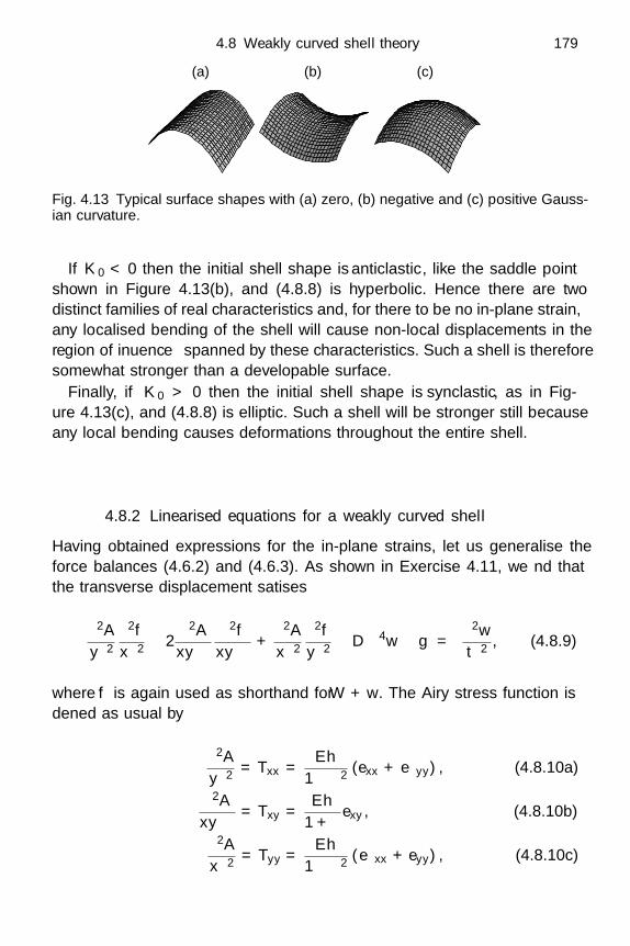
4.8 Weakly curved shell theory 179
(a) (b) (c)
Fig. 4.13 Typical surface shapes with (a) zero, (b) negative and (c) positive Gauss-ian curvature.
If K0 < 0 then the initial shell shape is anticlastic, like the saddle pointshown in Figure 4.13(b), and (4.8.8) is hyperbolic. Hence there are twodistinct families of real characteristics and, for there to be no in-plane strain,any localised bending of the shell will cause non-local displacements in theregion of influence spanned by these characteristics. Such a shell is thereforesomewhat stronger than a developable surface.
Finally, if K0 > 0 then the initial shell shape is synclastic, as in Fig-ure 4.13(c), and (4.8.8) is elliptic. Such a shell will be stronger still becauseany local bending causes deformations throughout the entire shell.
4.8.2 Linearised equations for a weakly curved shell
Having obtained expressions for the in-plane strains, let us generalise theforce balances (4.6.2) and (4.6.3). As shown in Exercise 4.11, we find thatthe transverse displacement satisfies
∂2A
∂y2∂2f
∂x2 − 2∂2A
∂x∂y
∂2f
∂x∂y+
∂2A
∂x2∂2f
∂y2 − D∇4w − ςg = ς∂2w
∂t2, (4.8.9)
where f is again used as shorthand for W + w. The Airy stress function isdefined as usual by
∂2A
∂y2 = Txx =Eh
1 − ν2 (exx + νeyy) , (4.8.10a)
− ∂2A
∂x∂y= Txy =
Eh
1 + νexy, (4.8.10b)
∂2A
∂x2 = Tyy =Eh
1 − ν2 (νexx + eyy) , (4.8.10c)

180 Approximate theories
with the strain components now given by (4.8.5). By eliminating the in-planedisplacement (u, v) between these, we find that A now satisfies
∇4A = Eh
∂2W
∂x2∂2W
∂y2 −(
∂2W
∂x∂y
)2
− ∂2f
∂x2∂2f
∂y2 +(
∂2f
∂x∂y
)2
. (4.8.11)
In (4.8.9) and (4.8.11) we have two equations for A and w, generalising thevon Karman equations, which may be recovered by setting W ≡ 0, f ≡ w.To make the model more tractable, let us now suppose that the transversedisplacement is much smaller than the initial deflection of the centre-surface,so that w W . Then, if we keep only the lowest order terms in w, (4.8.9)and (4.8.11) reduce to
∂2W
∂y2∂2A
∂x2 − 2∂2W
∂x∂y
∂2A
∂x∂y+
∂2W
∂x2∂2A
∂y2 = D∇4w, (4.8.12)
∂2W
∂y2∂2w
∂x2 − 2∂2W
∂x∂y
∂2w
∂x∂y+
∂2W
∂x2∂2w
∂y2 = −(Eh)−1∇4A, (4.8.13)
where, for additional simplicity, we have also neglected the body force andtime dependence. Given the initial shell profile W (x, y), we therefore havea coupled system of linear partial differential equations governing the smalltransverse displacement w and the Airy stress function A.
4.8.3 Solutions for a thin shell
Let us consider a shell whose initial shape W (x, y) is of order W0. We firsttry making the variables dimensionless in (4.8.12), (4.8.13) as follows:
x = Lx′, y = Ly′, W = W0W′, w = w0w
′, A =Dw0
W0A′, (4.8.14)
where L is a typical lateral dimension, and w0 a typical boundary displace-ment. We obtain, after suppressing primes,
∂2W
∂y2∂2A
∂x2 − 2∂2W
∂x∂y
∂2A
∂x∂y+
∂2W
∂x2∂2A
∂y2 = ∇4w, (4.8.15)
∂2W
∂y2∂2w
∂x2 − 2∂2W
∂x∂y
∂2w
∂x∂y+
∂2W
∂x2∂2w
∂y2 = −δ∇4A, (4.8.16)
where
δ =h2
12(1 − ν2)W 20
. (4.8.17)
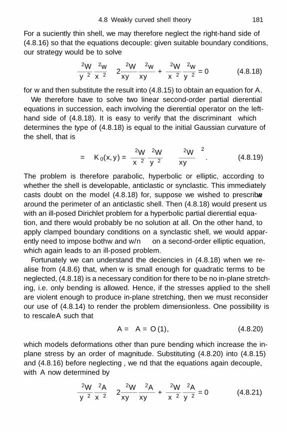
4.8 Weakly curved shell theory 181
For a sufficiently thin shell, we may therefore neglect the right-hand side of(4.8.16) so that the equations decouple: given suitable boundary conditions,our strategy would be to solve
∂2W
∂y2∂2w
∂x2 − 2∂2W
∂x∂y
∂2w
∂x∂y+
∂2W
∂x2∂2w
∂y2 = 0 (4.8.18)
for w and then substitute the result into (4.8.15) to obtain an equation for A.We therefore have to solve two linear second-order partial differential
equations in succession, each involving the differential operator on the left-hand side of (4.8.18). It is easy to verify that the discriminant ∆ whichdetermines the type of (4.8.18) is equal to the initial Gaussian curvature ofthe shell, that is
∆ = K0(x, y) =∂2W
∂x2∂2W
∂y2 −(
∂2W
∂x∂y
)2
. (4.8.19)
The problem is therefore parabolic, hyperbolic or elliptic, according towhether the shell is developable, anticlastic or synclastic. This immediatelycasts doubt on the model (4.8.18) for, suppose we wished to prescribe w
around the perimeter of an anticlastic shell. Then (4.8.18) would present uswith an ill-posed Dirichlet problem for a hyperbolic partial differential equa-tion, and there would probably be no solution at all. On the other hand, toapply clamped boundary conditions on a synclastic shell, we would appar-ently need to impose both w and ∂w/∂n on a second-order elliptic equation,which again leads to an ill-posed problem.
Fortunately we can understand the deficiencies in (4.8.18) when we re-alise from (4.8.6) that, when w is small enough for quadratic terms to beneglected, (4.8.18) is a necessary condition for there to be no in-plane stretch-ing, i.e. only bending is allowed. Hence, if the stresses applied to the shellare violent enough to produce in-plane stretching, then we must reconsiderour use of (4.8.14) to render the problem dimensionless. One possibility isto rescale A such that
A = δA = O (1), (4.8.20)
which models deformations other than pure bending which increase the in-plane stress by an order of magnitude. Substituting (4.8.20) into (4.8.15)and (4.8.16) before neglecting δ, we find that the equations again decouple,with A now determined by
∂2W
∂y2∂2A
∂x2 − 2∂2W
∂x∂y
∂2A
∂x∂y+
∂2W
∂x2∂2A
∂y2 = 0 (4.8.21)
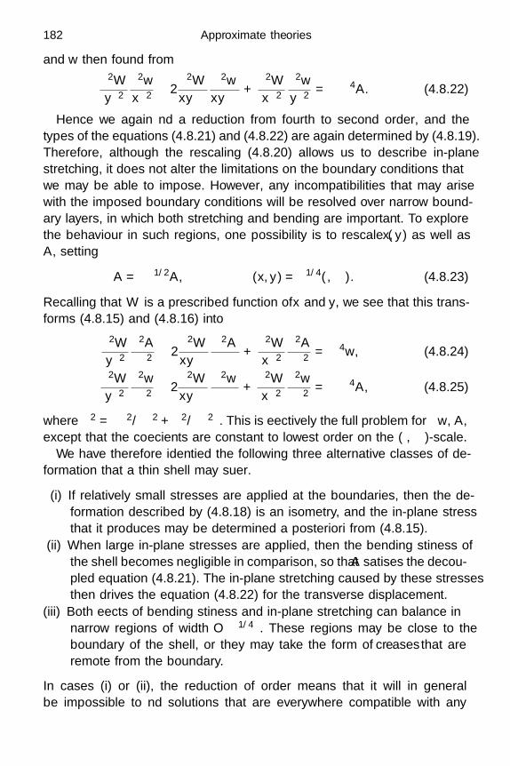
182 Approximate theories
and w then found from
∂2W
∂y2∂2w
∂x2 − 2∂2W
∂x∂y
∂2w
∂x∂y+
∂2W
∂x2∂2w
∂y2 = −∇4A. (4.8.22)
Hence we again find a reduction from fourth to second order, and thetypes of the equations (4.8.21) and (4.8.22) are again determined by (4.8.19).Therefore, although the rescaling (4.8.20) allows us to describe in-planestretching, it does not alter the limitations on the boundary conditions thatwe may be able to impose. However, any incompatibilities that may arisewith the imposed boundary conditions will be resolved over narrow bound-ary layers, in which both stretching and bending are important. To explorethe behaviour in such regions, one possibility is to rescale (x, y) as well asA, setting
A = δ−1/2A, (x, y) = δ1/4(ξ, η). (4.8.23)
Recalling that W is a prescribed function of x and y, we see that this trans-forms (4.8.15) and (4.8.16) into
∂2W
∂y2∂2A
∂ξ2 − 2∂2W
∂x∂y
∂2A
∂ξ∂η+
∂2W
∂x2∂2A
∂η2 = ∇4w, (4.8.24)
∂2W
∂y2∂2w
∂ξ2 − 2∂2W
∂x∂y
∂2w
∂ξ∂η+
∂2W
∂x2∂2w
∂η2 = −∇4A, (4.8.25)
where ∇2 =(∂2/∂ξ2 + ∂2/∂η2
). This is effectively the full problem for w, A,
except that the coefficients are constant to lowest order on the (ξ, η)-scale.We have therefore identified the following three alternative classes of de-
formation that a thin shell may suffer.
(i) If relatively small stresses are applied at the boundaries, then the de-formation described by (4.8.18) is an isometry, and the in-plane stressthat it produces may be determined a posteriori from (4.8.15).
(ii) When large in-plane stresses are applied, then the bending stiffness ofthe shell becomes negligible in comparison, so that A satisfies the decou-pled equation (4.8.21). The in-plane stretching caused by these stressesthen drives the equation (4.8.22) for the transverse displacement.
(iii) Both effects of bending stiffness and in-plane stretching can balance innarrow regions of width O
(δ1/4
). These regions may be close to the
boundary of the shell, or they may take the form of creases that areremote from the boundary.
In cases (i) or (ii), the reduction of order means that it will in generalbe impossible to find solutions that are everywhere compatible with any
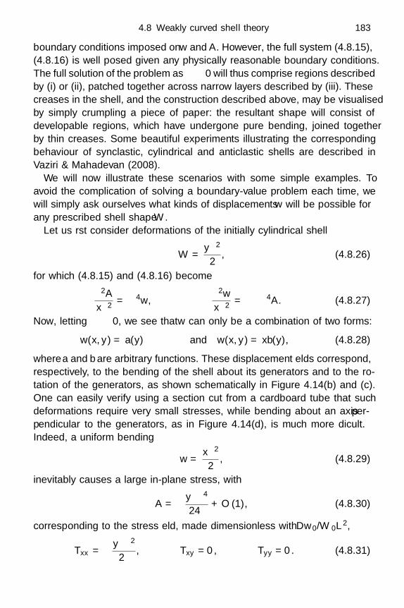
4.8 Weakly curved shell theory 183
boundary conditions imposed on w and A. However, the full system (4.8.15),(4.8.16) is well posed given any physically reasonable boundary conditions.The full solution of the problem as δ → 0 will thus comprise regions describedby (i) or (ii), patched together across narrow layers described by (iii). Thesecreases in the shell, and the construction described above, may be visualisedby simply crumpling a piece of paper: the resultant shape will consist ofdevelopable regions, which have undergone pure bending, joined togetherby thin creases. Some beautiful experiments illustrating the correspondingbehaviour of synclastic, cylindrical and anticlastic shells are described inVaziri & Mahadevan (2008).
We will now illustrate these scenarios with some simple examples. Toavoid the complication of solving a boundary-value problem each time, wewill simply ask ourselves what kinds of displacements w will be possible forany prescribed shell shape W .
Let us first consider deformations of the initially cylindrical shell
W =αy2
2, (4.8.26)
for which (4.8.15) and (4.8.16) become
α∂2A
∂x2 = ∇4w, α∂2w
∂x2 = −δ∇4A. (4.8.27)
Now, letting δ → 0, we see that w can only be a combination of two forms:
w(x, y) = a(y) and w(x, y) = xb(y), (4.8.28)
where a and b are arbitrary functions. These displacement fields correspond,respectively, to the bending of the shell about its generators and to the ro-tation of the generators, as shown schematically in Figure 4.14(b) and (c).One can easily verify using a section cut from a cardboard tube that suchdeformations require very small stresses, while bending about an axis per-pendicular to the generators, as in Figure 4.14(d), is much more difficult.Indeed, a uniform bending
w =βx2
2, (4.8.29)
inevitably causes a large in-plane stress, with
A = −αβy4
24δ+ O (1), (4.8.30)
corresponding to the stress field, made dimensionless with Dw0/W0L2,
Txx = −αβy2
2δ, Txy = 0, Tyy = 0. (4.8.31)
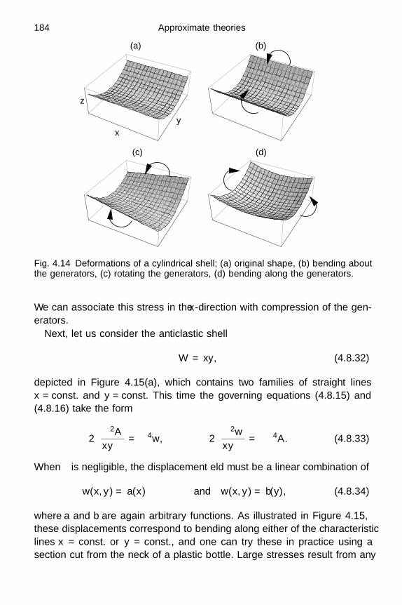
184 Approximate theories
x
y
z
(a) (b)
(d)(c)
Fig. 4.14 Deformations of a cylindrical shell; (a) original shape, (b) bending aboutthe generators, (c) rotating the generators, (d) bending along the generators.
We can associate this stress in the x-direction with compression of the gen-erators.
Next, let us consider the anticlastic shell
W = αxy, (4.8.32)
depicted in Figure 4.15(a), which contains two families of straight linesx = const. and y = const. This time the governing equations (4.8.15) and(4.8.16) take the form
−2α∂2A
∂x∂y= ∇4w, 2α
∂2w
∂x∂y= δ∇4A. (4.8.33)
When δ is negligible, the displacement field must be a linear combination of
w(x, y) = a(x) and w(x, y) = b(y), (4.8.34)
where a and b are again arbitrary functions. As illustrated in Figure 4.15,these displacements correspond to bending along either of the characteristiclines x = const. or y = const., and one can try these in practice using asection cut from the neck of a plastic bottle. Large stresses result from any

4.8 Weakly curved shell theory 185
x
y
z
(a) (b)
(d)(c)
Fig. 4.15 Deformations of an anticlastic shell; (a) original shape, (b) bending alongthe lines x = const., (c) bending along the lines y = const., (d) bending along thelines x − y = const.
other transverse displacement. For example,
w =β(x + y)2
2, (4.8.35)
which represents bending at an angle of π/4 to the coordinate axes, as shownin Figure 4.15(d), leads to a stress function
A =αβ
24δ
(x4 + y4)+ O (1). (4.8.36)
The corresponding dimensionless stress field
Txx =αβy2
2δ, Txy = 0, Tyy =
αβx2
2δ(4.8.37)
shows that both the normal stresses increase quadratically. due to stretchingof the straight lines x = const. and y = const. respectively.
Finally, let us consider the synclastic shell
W =α(x2 + y2
)2
. (4.8.38)

186 Approximate theories
x
y
z
(a) (b)
(d)(c)
Fig. 4.16 Deformations of a synclastic shell; (a) original shape, (b) and (c) twopossible deformations, (d) one-dimensional bending.
As may be seen in Figure 4.16(a), there are no straight lines embedded inthis surface. The governing equations (4.8.15) and (4.8.13) read
α∇2A = ∇4w, α∇2w = −δ∇4A, (4.8.39)
so that, when δ is small, only harmonic displacement fields are possible.Some examples are
w(x, y) = β(x2 − y2) and w(x, y) = −
β(x4 − 6x2y2 + y4
)4
, (4.8.40)
which are illustrated in Figure 4.16(b) and (c) respectively. In the first, theshell is bent upwards in the x-direction and downwards in the y-direction; inthe second, the corners are bent upwards and the edges downwards. Thesecan easily be realised using a segment from a ping-pong ball. On the otherhand, if we perform the rescaling (4.8.20) before letting δ → 0, we find thatA satisfies Laplace’s equation and thus
α∇2w = −∇4A = 0. (4.8.41)
Hence, any non-harmonic displacement field, for example the one-dimensionalbending w = βx2 illustrated in Figure 4.16, does not just give rise to largein-plane stress but is actually impossible. If we tried to impose boundary

4.9 Nonlinear beam theory 187
conditions that force such a one-dimensional bending response, we wouldinevitably cause a crease to be formed.
Although the above theory only applies to very small transverse displace-ments of shells whose built-in curvature is already small, it illustrates manyof the key differences between the elastic responses of shells and plates. Anytheory for more general shells demands more differential geometry than wecan conveniently introduce in this chapter, and we will return to this topic inChapter 6. We can, however, consider nearly one-dimensional elastic bodieswith arbitrary curvature, and this we do in the next section.
4.9 Nonlinear beam theory
4.9.1 Derivation of the model
We now return to the beam configuration considered in Section 4.4, now gen-eralising the model to make it applicable to commonly observed phenomenasuch as the deflection of a diving board. Diving boards undergo large dis-placement without any of the damaging effects that are associated with largestrains. This is possible because a thin elastic beam can be bent without sig-nificantly stretching its centre-line, as illustrated in Figure 4.17(a,b). Theinternal displacement field in such a beam is shown schematically in Fig-ure 4.17(c): the net effect is to stretch the outer surface of the beam andcompress the inner surface, while the length of the centre-line is virtuallyunchanged. It is an elementary exercise in trigonometry to show that the
h
R
(a)
(c)(b)
Fig. 4.17 A beam (a) before and (b) after bending; (c) a close-up of the displacementfield.

188 Approximate theories
N0
T0
T0
N0(a) (b)
θM(s + δs)
T (s + δs)
N(s + δs)
T (s)
N(s)
M(s)
Fig. 4.18 (a) The forces and moments acting on a small segment of a beam. (b) Thesign convention for the forces at the ends of the beam.
strain associated with such a displacement is of order h/R, where h is thethickness of the beam and R the radius of curvature through which it isbent. Provided the beam is sufficiently thin, it can therefore suffer largedisplacements while the internal strain remains small. As noted above inSection 4.8, a developable shell has the same property when bent about itsgenerators.
If the strain is small, then we can still assume that the stress is a linearfunction of the strain. However, when the displacement is large, linear elas-ticity is no longer valid: the Eulerian and Lagrangian coordinates are farfrom interchangeable, and it is not legitimate to linearise the relationshipbetween strain and displacement. We therefore seek a geometrically non-linear but mechanically linear theory, in a similar vein to the von Karmanplate theory from Section 4.7.
In equilibrium, it is surprisingly easy to generalise our derivation of lin-ear beam theory in Section 4.4 to model large two-dimensional transversedisplacements. We describe the deformation of the beam using arc-lengths along the centre-line and the angle θ(s) between the centre-line and thex-axis. As discussed above, we assume the centre-line to be inextensible toleading order, so that arc-length is conserved by the deformation and we canthus view s as a Lagrangian coordinate that is fixed in the deforming beam.The transverse displacement is given parametrically by x = x(s), w = w(s),where
dx
ds= cos θ,
dw
ds= sin θ. (4.9.1)
Now we balance forces and moments on a small segment of the beam asshown in Figure 4.18(a). We neglect inertia and body forces for the moment
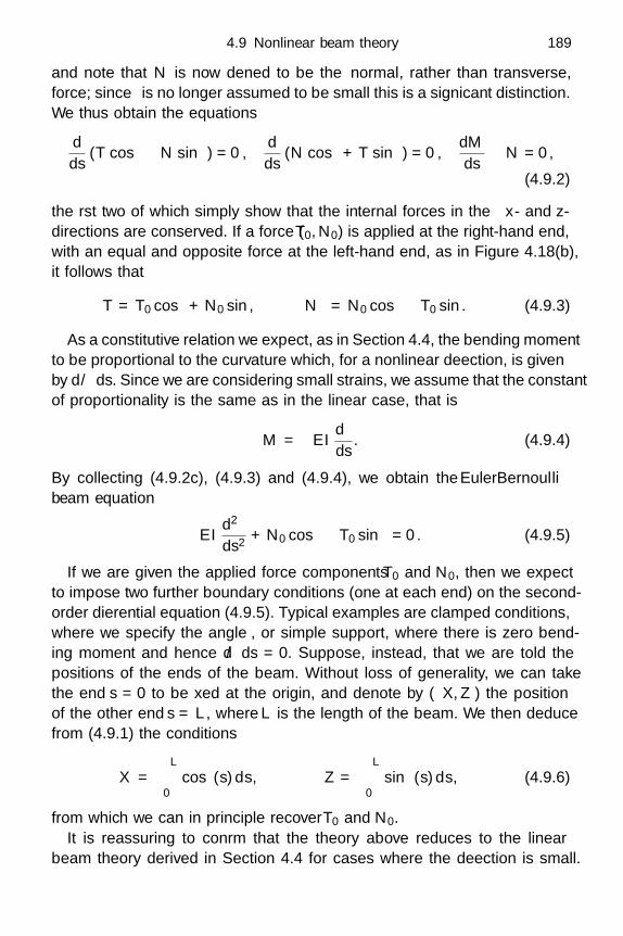
4.9 Nonlinear beam theory 189
and note that N is now defined to be the normal, rather than transverse,force; since θ is no longer assumed to be small this is a significant distinction.We thus obtain the equations
dds
(T cos θ − N sin θ) = 0,dds
(N cos θ + T sin θ) = 0,dM
ds− N = 0,
(4.9.2)
the first two of which simply show that the internal forces in the x- and z-directions are conserved. If a force (T0, N0) is applied at the right-hand end,with an equal and opposite force at the left-hand end, as in Figure 4.18(b),it follows that
T = T0 cos θ + N0 sin θ, N = N0 cos θ − T0 sin θ. (4.9.3)
As a constitutive relation we expect, as in Section 4.4, the bending momentto be proportional to the curvature which, for a nonlinear deflection, is givenby dθ/ds. Since we are considering small strains, we assume that the constantof proportionality is the same as in the linear case, that is
M = −EIdθ
ds. (4.9.4)
By collecting (4.9.2c), (4.9.3) and (4.9.4), we obtain the Euler–Bernoullibeam equation
EId2θ
ds2 + N0 cos θ − T0 sin θ = 0. (4.9.5)
If we are given the applied force components T0 and N0, then we expectto impose two further boundary conditions (one at each end) on the second-order differential equation (4.9.5). Typical examples are clamped conditions,where we specify the angle θ, or simple support, where there is zero bend-ing moment and hence dθ/ds = 0. Suppose, instead, that we are told thepositions of the ends of the beam. Without loss of generality, we can takethe end s = 0 to be fixed at the origin, and denote by (X, Z) the positionof the other end s = L, where L is the length of the beam. We then deducefrom (4.9.1) the conditions
X =∫ L
0cos θ(s) ds, Z =
∫ L
0sin θ(s) ds, (4.9.6)
from which we can in principle recover T0 and N0.It is reassuring to confirm that the theory above reduces to the linear
beam theory derived in Section 4.4 for cases where the deflection is small.

190 Approximate theories
For small θ, we can simplify the geometric relations (4.9.1) to lowest orderto give
x = s,dw
dx= θ, (4.9.7)
and (4.9.5) thus becomes
EId3w
dx3 + N0 − T0dw
dx= 0. (4.9.8)
One further x-derivative reproduces the linear beam equation (4.4.8) in theabsence of inertia and gravity.
4.9.2 Example: deflection of a diving board
Under a shift in the origin of θ, (4.9.5) is equivalent to the equation for apendulum whose small-amplitude frequency of oscillation is
√T 2
0 + N20 /EI.
However, in (4.9.5), s is far from being a time-like variable, and the typicalboundary conditions discussed above are quite different from the sort ofinitial conditions we would expect to apply to a pendulum. However, we canuse techniques that are familiar from the study of pendulums to constructsolutions of (4.9.5).
Let us first consider the example, alluded to previously, of the steadydeformation of a diving board, with gravity neglected for simplicity. If theboard is clamped horizontally at s = 0 and a downward load F is appliedto the other end, which is otherwise free, then we have T0 = 0, N0 = −F
and (4.9.5) becomes
EId2θ
ds2 = F cos θ, (4.9.9)
subject to
θ(0) = 0,dθ
ds(L) = 0. (4.9.10)
Multiplying (4.9.9) through by dθ/ds and integrating once with respectto s, we obtain (
dθ
ds
)2
=2F
EI(sin θ − sinα) , (4.9.11)
where α is shorthand for −θ(L). When taking the square root, we note thatwe expect dθ/ds to be negative and thus obtain the solution in parametricform as ∫ −θ
0
dφ√sinα − sinφ
= s
√2F
EI. (4.9.12)
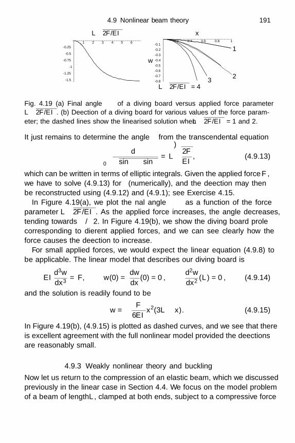
4.9 Nonlinear beam theory 191
1 2 3 4 5 6
-1.5
-1.25
-1
-0.75
-0.5
-0.25
0.2 0.4 0.6 0.8 1
-0.8
-0.7
-0.6
-0.5
-0.4
-0.3
-0.2
-0.1
x
−α
L√
2F/EI
w
1
3L√
2F/EI = 4
2
Fig. 4.19 (a) Final angle −α of a diving board versus applied force parameterL√
2F/EI. (b) Deflection of a diving board for various values of the force param-eter; the dashed lines show the linearised solution when L
√2F/EI = 1 and 2.
It just remains to determine the angle α from the transcendental equation∫ α
0
dφ√sin α − sinφ
= L
√2F
EI, (4.9.13)
which can be written in terms of elliptic integrals. Given the applied force F ,we have to solve (4.9.13) for α (numerically), and the deflection may thenbe reconstructed using (4.9.12) and (4.9.1); see Exercise 4.15.
In Figure 4.19(a), we plot the final angle −α as a function of the forceparameter L
√2F/EI. As the applied force increases, the angle decreases,
tending towards −π/2. In Figure 4.19(b), we show the diving board profilecorresponding to different applied forces, and we can see clearly how theforce causes the deflection to increase.
For small applied forces, we would expect the linear equation (4.9.8) tobe applicable. The linear model that describes our diving board is
EId3w
dx3 = F, w(0) =dw
dx(0) = 0,
d2w
dx2 (L) = 0, (4.9.14)
and the solution is readily found to be
w = − F
6EIx2(3L − x). (4.9.15)
In Figure 4.19(b), (4.9.15) is plotted as dashed curves, and we see that thereis excellent agreement with the full nonlinear model provided the deflectionsare reasonably small.
4.9.3 Weakly nonlinear theory and buckling
Now let us return to the compression of an elastic beam, which we discussedpreviously in the linear case in Section 4.4. We focus on the model problemof a beam of length L, clamped at both ends, subject to a compressive force
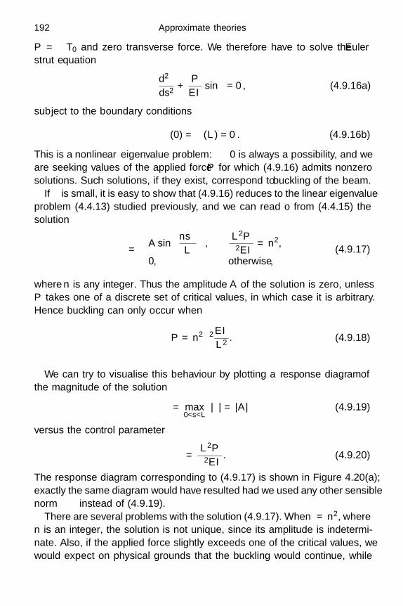
192 Approximate theories
P = −T0 and zero transverse force. We therefore have to solve the Eulerstrut equation
d2θ
ds2 +P
EIsin θ = 0, (4.9.16a)
subject to the boundary conditions
θ (0) = θ (L) = 0. (4.9.16b)
This is a nonlinear eigenvalue problem: θ ≡ 0 is always a possibility, and weare seeking values of the applied force P for which (4.9.16) admits nonzerosolutions. Such solutions, if they exist, correspond to buckling of the beam.
If θ is small, it is easy to show that (4.9.16) reduces to the linear eigenvalueproblem (4.4.13) studied previously, and we can read off from (4.4.15) thesolution
θ =
A sin(nπs
L
),
L2P
π2EI= n2,
0, otherwise,(4.9.17)
where n is any integer. Thus the amplitude A of the solution is zero, unlessP takes one of a discrete set of critical values, in which case it is arbitrary.Hence buckling can only occur when
P = n2π2 EI
L2 . (4.9.18)
We can try to visualise this behaviour by plotting a response diagram ofthe magnitude of the solution
‖θ‖ = max0<s<L
|θ| = |A| (4.9.19)
versus the control parameter
λ =L2P
π2EI. (4.9.20)
The response diagram corresponding to (4.9.17) is shown in Figure 4.20(a);exactly the same diagram would have resulted had we used any other sensiblenorm ‖θ‖ instead of (4.9.19).
There are several problems with the solution (4.9.17). When λ = n2, wheren is an integer, the solution is not unique, since its amplitude is indetermi-nate. Also, if the applied force slightly exceeds one of the critical values, wewould expect on physical grounds that the buckling would continue, while
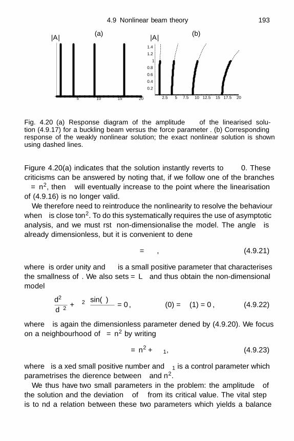
4.9 Nonlinear beam theory 193
5 10 15 20 2.5 5 7.5 10 12.5 15 17.5 20
0.2
0.4
0.6
0.8
1
1.2
1.4
λ λ
|A||A| (a) (b)
Fig. 4.20 (a) Response diagram of the amplitude ‖θ‖ of the linearised solu-tion (4.9.17) for a buckling beam versus the force parameter λ. (b) Correspondingresponse of the weakly nonlinear solution; the exact nonlinear solution is shownusing dashed lines.
Figure 4.20(a) indicates that the solution instantly reverts to θ ≡ 0. Thesecriticisms can be answered by noting that, if we follow one of the branchesλ = n2, then θ will eventually increase to the point where the linearisationof (4.9.16) is no longer valid.
We therefore need to reintroduce the nonlinearity to resolve the behaviourwhen λ is close to n2. To do this systematically requires the use of asymptoticanalysis, and we must first non-dimensionalise the model. The angle θ isalready dimensionless, but it is convenient to define
θ = δΘ, (4.9.21)
where Θ is order unity and δ is a small positive parameter that characterisesthe smallness of θ. We also set s = Lξ and thus obtain the non-dimensionalmodel
d2Θdξ2 + π2λ
sin(δΘ)δ
= 0, θ (0) = θ (1) = 0, (4.9.22)
where λ is again the dimensionless parameter defined by (4.9.20). We focuson a neighbourhood of λ = n2 by writing
λ = n2 + ελ1, (4.9.23)
where ε is a fixed small positive number and λ1 is a control parameter whichparametrises the difference between λ and n2.
We thus have two small parameters in the problem: the amplitude δ ofthe solution and the deviation ε of λ from its critical value. The vital stepis to find a relation between these two parameters which yields a balance

194 Approximate theories
between the compressive loading, characterised by ε, and the nonlinearity,characterised by δ, and the correct choice leads to a so-called weakly non-linear theory. If we use the assumed smallness of δ to expand the sine in(4.9.22), we obtain the Duffing equation
d2Θdξ2 + π2 (n2 + ελ1
)(Θ − δ2 Θ3
6+ · · ·
)= 0, (4.9.24)
and we clearly see that the required balance is obtained by choosing
δ =√
ε. (4.9.25)
Before doing any further calculation, we can already infer from this that theamplitude of the solution will vary as the square root of the excess loading.
After making the choice (4.9.25), we write Θ as an asymptotic expansionof the form†
Θ ∼ Θ0 (ξ) + εΘ1 (ξ) + · · · . (4.9.26)
By substituting (4.9.26) into (4.9.24) and equating successive powers of ε,we find that
d2Θ0
dξ2 + n2π2Θ0 = 0, Θ0 (0) = Θ0 (1) = 0, (4.9.27a)
d2Θ1
dξ2 + n2π2Θ1 = −π2λ1Θ0 + n2π2 Θ30
6, Θ1 (0) = Θ1 (1) = 0. (4.9.27b)
The general solution of (4.9.27a) is
Θ0 = A0 sin (nπξ) , (4.9.28)
and we seem to have made very little progress from (4.9.17). However, whenwe examine the problem for Θ1, we find that (4.9.27b) has no solutionsunless the right-hand side satisfies a solvability condition, namely∫ 1
0
(λ1Θ0 − n2 Θ3
06
)sin (nπξ) dξ = 0. (4.9.29)
By substituting for Θ0 from (4.9.28), we obtain the following equation forthe leading-order amplitude:
A0
(A2
0 −8λ1
n2
)= 0. (4.9.30)
When λ1 is negative, the only real solution of (4.9.30) is A0 = 0 but, forpositive values of λ1, there are three such solutions: A0 = 0,±(2/n)
√2λ1.
†see Hinch (1991), for example, for the definition of an asymptotic expansion; for the purposesof this chapter, we can interpret ∼ as meaning approximates increasingly well as ε → 0

4.10 Nonlinear rod theory 195
A0
λ1
A0
λ1
stable
stable
unstablestable
(a) (b)
Fig. 4.21 (a) Pitchfork bifurcation diagram of leading-order amplitude A0 versusforcing parameter λ1 . (b) The corresponding diagram when asymmetry is intro-duced.
This behaviour of A0 as a function of λ1, depicted in Figure 4.21(a), ischaracteristic of a so-called pitchfork bifurcation.
Working backwards, we can easily turn (4.9.30) into an equation for theamplitude of θ; that is,
|A|[|A|2 − 8
(λ
n2 − 1)]
= 0, (4.9.31)
and this weakly nonlinear response is plotted in Figure 4.20(b). This givesthe physically expected result that the amplitude of each buckled solutionincreases with the excess applied force. We can also see how Figure 4.20(a)approximates this response for very small |A|. For comparison, we also showthe response of the full nonlinear solution of (4.9.16); see Exercise 4.18.
We can use the argument after (4.4.18) to show that the solution θ = 0 isstable for λ1 < 0 but loses stability to the nonzero solution as λ1 crosses zero.This justifies the labelling in Figure 4.21(a) and can also be explained onthe basis of an energy argument, as in Exercise 4.14. Another key ingredientof bifurcation pictures like Figure 4.21(a) is the symmetry that we haveassumed in our strut model. Any imperfection or asymmetry in the modelwould deform the response diagram into something like Figure 4.21(b), inwhich there is a smooth dependence of the solution on the control parameter.This is exemplified by the re-introduction of gravity in the model as inExercise 4.16.
4.10 Nonlinear rod theory
We are now in a position to generalise and combine the linear rod theory ofSection 4.5 with the nonlinear beam theory of Section 4.9 to derive a modelfor the equilibrium of a rod that can both twist about its tangent vector

196 Approximate theories
and bend in two perpendicular directions. We let F and M denote the forceand moment exerted on any cross-section s = const. of the rod, s beingarc-length along the centre-line. As in Section 4.9, we will assume that therod is inextensible so that s is effectively a Lagrangian variable. Neglectingbody forces for simplicity, a force balance gives
dF
ds= 0, so that F = F 0 = const.. (4.10.1)
This equation generalises the first two equations of (4.9.2). Also, if r(s)parametrises the centre-line of the rod, then a moment balance analogousto the final equation of (4.9.2) gives
dM
ds+(
dr
ds×F
)= 0, so that M + r×F 0 = M 0 = const.. (4.10.2)
The equations (4.10.1), (4.10.2) for the vectors F , M and r now needto be closed by a constitutive law for M , and this is what poses the mostinteresting modelling challenge. Instead of adopting the usual differentialgeometry definition of curvature, we consider what happens to a Lagrangianorthonormal system ei(s) (i = 1, 2, 3) as the rod deforms. This system isfixed in the rod and we choose
e1(s) =dr
ds, (4.10.3)
with e2 and e3 defining the normal plane. At different s-stations, this systemwill have rotated by different amounts, and we infer that there exists a vectorΩ(s) such that
dei
ds= Ω(s)×ei(s). (4.10.4)
Thinking of s as time for the moment, the vector Ω = (Ω1, Ω2, Ω3)T
represents the “angular velocity” of the orthonormal system e1, e2, e3,with Ω1 corresponding to twisting of the rod about its axis and Ω2, Ω3 tobending. This leads us to propose a linear constitutive relation between M
and Ω, so that
M = BΩ (4.10.5)
for some 3 × 3 matrix B, whose elements we will choose to ensure that(4.10.5) agrees with (4.5.5), (4.5.9) and (4.9.4) in the appropriate limits.
In linear rod theory, we write r =(x, v(x), w(x)
)T, where x = s to lowestorder. When we neglect quadratic terms, the orthonormal vectors ei may be
4.10 Nonlinear rod theory 197
written in the form
e1 =(
1,dv
dx,dw
dx
)T
, e2 =(−dv
dx, 1, θ
)T
, e3 =(−dw
dx,−θ, 1
)T
,
(4.10.6)
where θ measures the twist of the rod about the x-axis. It is easy to checkthat these are consistent with (4.10.4) and correspond to
Ω =(
dθ
dx,−d2w
dx2 ,d2v
dx2
)T
. (4.10.7)
Now we see that we can reproduce (4.5.5) and (4.5.9) by choosing
B =
R 0 00 EIyy −EIyz
0 −EIyz EIzz
, (4.10.8)
in the notation of Section 4.5.To retrieve nonlinear beam theory, we write r =
(x(s), 0, w(s)
)T, so that
e1 =
cos θ
0sin θ
, e2 =
010
, e1 =
− sin θ
0cos θ
, (4.10.9)
and we easily find that
Ω =(
0,dθ
ds, 0)T
. (4.10.10)
Provided the beam is symmetric so that Iyz = 0, (4.10.5) with B givenby (4.10.8) thus reduces to the constitutive relation (4.9.4) for a nonlinearbeam.
The relations (4.10.1)–(4.10.5) comprise a formidable system of 15 equa-tions for F , M , r, ei and Ω. Fortunately, there is a wonderful analogy thatrelieves us of the task of discussing the behaviour of this system. Considera rigid body rotating about a fixed origin 0 such that one principal axis e1
at 0 passes through the centre of gravity which is a distance h from 0. Theequations of motion for such a body are
dei
dt= ω×ei,
dH
dt= he1×W , H = Iω, (4.10.11)
where ω is the angular velocity, e2, e3 are the other principal axes, H isthe angular momentum, W is the weight and I the inertia tensor. Whenwe identify ω with Ω, H with M , hW with F and, crucially, s with t, theseequations are simply (4.10.4), (4.10.2) and (4.10.5). Hence our knowledge

198 Approximate theories
about spinning tops, gyroscopes and “inertia coupling” in classical mechan-ics can be used to explain the often infuriating coupling between torsionand bending that is only too familiar to those who have to wind cables andgarden hoses.
This Kirchhoff analogy disappears when we consider the dynamics of arod subject to a body force g, the model for which is precisely as above withd/ds replaced by ∂/∂s and (4.10.1) replaced by
ρ∂2r
∂t2= ρg +
∂F
∂s. (4.10.12)
4.11 Geometrically nonlinear wave propagation
When we include nonlinear effects in models for elastic wave propagation,we will rarely be able to find explicit solutions. Hence, in this section, wewill simply describe a few nonlinear models that are relatively easy to deriveand posess interesting exact solutions.
4.11.1 Gravity-torsional waves
Our first example of nonlinear wave propagation is a generalisation to includegravity in the model (4.5.8) for torsional waves in a rod. In particular, we willtry to model the waves that can propagate when a series of rigid pendulumsis attached to a rod which is stiff but has negligible mass. In practice, sucha configuration can be realised by attaching paper clips to a taut segmentof a rubber band, as shown in Figure 4.22, where the paper clips are drawnas pendulums.†
To model this situation, we suppose that each pendulum is acted upon bya moment δM at its point of support. A net moment balance, as illustratedin Figure 4.22(b), leads to
δM = mg sin θ + m2 ∂2θ
∂t2, (4.11.1)
where θ(x, t) is the angle between the pendulum and the downward verticalwhile m and are the mass and length of the pendulum respectively. Nowwe identify the moment δM with b∂M/∂x, where b is the spacing betweenthe pendulums and ∂M/∂x is given by the constitutive relation (4.5.9). Wetherefore find that θ satisfies
bR∂2θ
∂x2 = mg sin θ + m2 ∂2θ
∂t2, (4.11.2)
†We are grateful to the late Prof. T. Brooke Benjamin for drawing this experiment to ourattention.
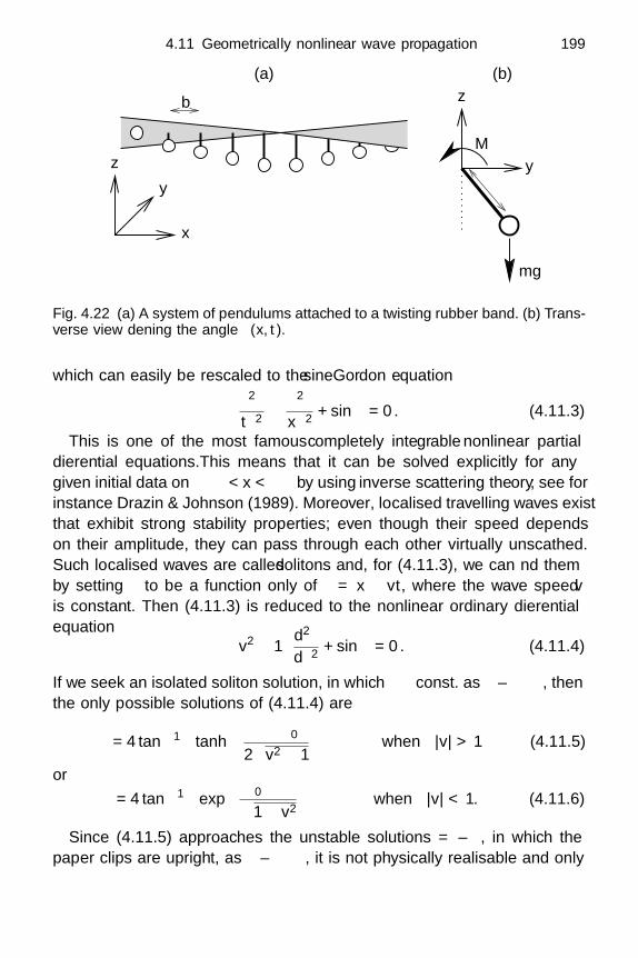
4.11 Geometrically nonlinear wave propagation 199
θ
mg
z
y
y
x
z
(b)(a)
δM
b
Fig. 4.22 (a) A system of pendulums attached to a twisting rubber band. (b) Trans-verse view defining the angle θ(x, t).
which can easily be rescaled to the sine–Gordon equation
∂2θ
∂t2− ∂2θ
∂x2 + sin θ = 0. (4.11.3)
This is one of the most famous completely integrable nonlinear partialdifferential equations.This means that it can be solved explicitly for anygiven initial data on −∞ < x < ∞ by using inverse scattering theory ; see forinstance Drazin & Johnson (1989). Moreover, localised travelling waves existthat exhibit strong stability properties; even though their speed dependson their amplitude, they can pass through each other virtually unscathed.Such localised waves are called solitons and, for (4.11.3), we can find themby setting θ to be a function only of η = x − vt, where the wave speed v
is constant. Then (4.11.3) is reduced to the nonlinear ordinary differentialequation (
v2 − 1) d2θ
dη2 + sin θ = 0. (4.11.4)
If we seek an isolated soliton solution, in which θ → const. as η → ±∞, thenthe only possible solutions of (4.11.4) are
θ = 4 tan−1
tanh(
η − η0
2√
v2 − 1
)when |v| > 1 (4.11.5)
orθ = 4 tan−1
exp
(η0 − η√1 − v2
)when |v| < 1. (4.11.6)
Since (4.11.5) approaches the unstable solutions θ = ±π, in which thepaper clips are upright, as η → ±∞, it is not physically realisable and only

200 Approximate theories
y
xz
t = 2t = 1t = 0
Fig. 4.23 A kink propagating along a series of pendulums attached to a rod.
the subsonic waves (4.11.6) can be observed in practice. In these so-calledkink solutions, the rod undergoes one complete twist, with θ = 0 ahead ofthe wave (η → +∞) and θ = 2π behind (η → −∞), as shown in Figure 4.23.They can easily be realised in the system illustrated in Figure 4.22 by hold-ing the rubber band tight and horizontal, with all the paper clips danglingvertically, and then quickly twisting one end through 2π.
4.11.2 Travelling waves on a beam
Our second example concerns the unsteady generalisation of the geometri-cally nonlinear beam theory derived in Section 4.9. The displacement of thebeam is now given parametrically by x = x(s, t), w = w(x, t), where, as in(4.9.1),
∂x
∂s= cos θ,
∂w
∂s= sin θ, (4.11.7)
and θ(s, t) is the angle made by the beam with the x-axis. When we includeacceleration, the force balances (4.9.2) become
∂
∂s(T cos θ − N sin θ) =
∂2x
∂t2,
∂
∂s(N cos θ + T sin θ) =
∂2w
∂t2, (4.11.8)
where
N = −EI∂2θ
∂s2 . (4.11.9)
Although this is a more complicated model than (4.11.3), we can still seeka travelling wave solution in which x, w, T , N and θ are functions only ofη = s − vt. We also postulate the boundary conditions
T → T∞, N → 0, θ → 0, x ∼ s, w → 0 as s → ∞, (4.11.10)
which would apply, for example, to a long taut rope that had been shakenbriefly at one end. As in Section 4.11.1, by looking for a travelling wave, wereduce (4.11.8) to nonlinear ordinary differential equations, which may be

4.11 Geometrically nonlinear wave propagation 201
-2 -1 1 2
-2
-1.5
-1
-0.5
wx
v
Fig. 4.24 Travelling wave solution of the nonlinear beam equations (with k = 1).
integrated to obtain
T cos θ − N sin θ = v2 (cos θ − 1) + T∞, T sin θ + N cos θ = v2 sin θ.
(4.11.11)
Hence the tension and shear force are given by
T = v2 +(T∞ − v2) cos θ, N =
(v2 − T∞
)sin θ, (4.11.12)
and (4.11.9) therefore becomes
EI
T∞
d2θ
dη2 +(M2 − 1
)sin θ = 0, (4.11.13)
where M = |v|√
/T∞. We recall from Chapter 3 that√
T∞/ is the phasevelocity of small-amplitude transverse waves on a string, and M is the Machnumber of the wave.
By analogy with (4.11.4), we see that, as long as M < 1, there is a solutionconnecting θ → 0 as η → +∞ to θ → 2π as η → −∞, namely
θ = 4 tan−1(ek(η0−η)
), where k =
√T∞EI
(1 − M2), (4.11.14)
where the constant η0 represents an arbitrary translation. With θ given by(4.11.14), we can integrate (4.11.7) to obtain the parametric description(
x
w
)=
1k
(ξ − 2 tanh ξ
−2 sech ξ
)(4.11.15)
for the shape of the rope, where ξ = k(η−η0). As shown in Figure 4.24, thisrepresents a single loop, in which the rope turns through 2π, propagatingat speed v which depends, through (4.11.14), on the amplitude. The multi-valuedness of w(x) is only physically realistic if the rope is allowed to deformslightly out of the (x, z)-plane.

202 Approximate theories
4.11.3 Weakly nonlinear waves on a beam
If we wish to analyse general unsteady deformations of a beam, we appear tobe confronted with the full system (4.11.7)–(4.11.9) of nonlinear equationsfor x, w, T , N and θ. However, we will now show that, when the solution isclose to a travelling wave, we can obtain a single partial differential equationincorporating all the ingredients of unsteadiness, dispersion and nonlinearity.Moreover, it will transpire that this equation is closely related to one of themost famous of all soliton equations.
We observe that (4.11.13) is degenerate when EI = 0 and M2 = 1:when the beam has zero bending stiffness, θ can be an arbitrary functionof s − ct. This motivates us to seek a “distinguished limit” in which thebending stiffness is small but nonzero and the wave is approximately movingat speed c =
√T∞/, where T∞ is the tension applied at infinity as before.
To analyse this limit, our first step is to express the equations in a movingreference frame, by transforming from (s, t) to (ζ, t), where ζ = s − ct, sothat (4.11.7)–(4.11.9) become
∂x
∂ζ= cos θ,
∂w
∂ζ= sin θ, N = −EI
∂2θ
∂ζ2 , (4.11.16)
∂
∂ζ
((T − T∞) cos θ − N sin θ
)=
(∂2x
∂t2− 2c
∂2x
∂ζ∂t
), (4.11.17)
∂
∂ζ
(N cos θ + (T − T∞) sin θ
)=
(∂2w
∂t2− 2c
∂2w
∂ζ∂t
). (4.11.18)
Now we have to non-dimensionalise the equations before we can take asystematic asymptotic limit. We denote by a typical amplitude of the waveand obtain a suitable scaling for N from (4.11.16). The relevant time-scaleis then found by balancing the final term in (4.11.17) with the normal stresson the left-hand side. We thus define the dimensionless variables asx
w
ζ
=
X
W
ξ
, T = T∞T , N =(
EI
2
)N , t =
(2c3
EI
)τ,
(4.11.19)
so that (4.11.16)–(4.11.18) become
∂X
∂ξ= cos θ,
∂W
∂ξ= sin θ, (4.11.20)
4.11 Geometrically nonlinear wave propagation 203
N = −∂2θ
∂ξ2 , (4.11.21)
∂
∂ξ
((T − 1) cos θ − εN sin θ
)=
ε2
4∂2X
∂τ 2 − ε∂2X
∂ξ∂τ, (4.11.22)
∂
∂ξ
(εN cos θ + (T − 1) sin θ
)=
ε2
4∂2W
∂τ 2 − ε∂2W
∂ξ∂τ, (4.11.23)
where the only remaining dimensionless parameter in the problem is
ε =EI
T∞2 . (4.11.24)
We suppose, as in Section 4.11.2, that the beam is held straight and hori-zontal, under a uniform tension at infinity, so that
T → 1, N → 0, θ → 0, X ∼ ξ, W → 0 as ξ → ∞. (4.11.25)
Now we take the limit ε → 0, which corresponds to the bending stiffnessof the beam being small. When ε = 0, (4.11.22) and (4.11.23) are satisfiedidentically by T = 1, and this motivates the ansatz
T ∼ 1 + εT1 + · · · . (4.11.26)
When we substitute (4.11.26) into (4.11.22) and (4.11.23) and let ε → 0, wefind that the leading-order equations may be integrated once with respectto ξ, using the boundary conditions (4.11.25), to obtain
T1 cos θ −N sin θ +∂X
∂τ= 0, T1 sin θ + N cos θ +
∂W
∂τ= 0. (4.11.27)
We solve these simultaneously for T1 and N and substitute into (4.11.21) toobtain
∂2θ
∂ξ2 +∂X
∂τsin θ − ∂W
∂τcos θ = 0, (4.11.28)
which is to be solved along with (4.11.20) for θ(ξ, τ), X(ξ, τ) and W (ξ, τ).A remarkable first integration is now possible which allows us to eliminate
X and W to obtain a single equation for θ. When we multiply (4.11.28) by∂θ/∂ξ we discover by virtue of (4.11.20) that it may be integrated withrespect to ξ, leading, from (4.11.25), to
∂X
∂τcos θ +
∂W
∂τsin θ =
12
(∂θ
∂ξ
)2
. (4.11.29)

204 Approximate theories
On the other hand, if we instead differentiate (4.11.28) with respect to ξ,again using (4.11.20), we find that
∂θ
∂ξ
(∂X
∂τcos θ +
∂W
∂τsin θ
)=
∂θ
∂τ− ∂3θ
∂ξ3 . (4.11.30)
Finally, comparing (4.11.29) and (4.11.30), we obtain
∂θ
∂τ− 1
2
(∂θ
∂ξ
)3
− ∂3θ
∂ξ3 = 0. (4.11.31)
If we differentiate (4.11.31) with respect to ξ, we find that the equationsatisfied by ∂θ/∂ξ is a version of the modified KdV equation, which can itselfbe transformed into the celebrated KdV equation (see Exercise 4.20). TheKdV equation was originally used to model large-amplitude water waves,and its study provided a key stimulus for the theory of solitons.
By reversing the scalings (4.11.19), we obtain the dimensional version of(4.11.31), namely
2T∞EI
(1c
∂θ
∂t+
∂θ
∂s
)− 1
2
(∂θ
∂s
)3
− ∂3θ
∂s3 = 0. (4.11.32)
Now if we seek a travelling wave, in which θ is again a function only ofη = s − V t, then we obtain the ordinary differential equation
d3θ
dη3 +12
(dθ
dη
)3
− 2T∞EI
(1 − M)dθ
dη= 0, (4.11.33)
where M = V/c again. As shown in Exercise 4.21, the solution of this equa-tion satisfying θ → 0 as η → +∞ and θ → 2π as η → −∞ is
θ = 4 tan−1(eκ(η0−η)
), where κ =
√2T∞(1 − M)
EI. (4.11.34)
We thus reproduce the travelling wave solution (4.11.14) found previously,noting that κ is the leading-order approximation to k as M → 1.
4.12 Concluding remarks
In this chapter, we have emphasised phenomena that can occur when thereis some strong geometric constraint of “thinness”, and hence the possibil-ity of geometric nonlinearity. However, what is more remarkable than thephenomena themselves is the mathematical challenge posed by passing froma fully three-dimensional model to simpler models for nearly one- or two-dimensional solids. This challenge is exemplified by the fact that, although(4.3.2) is an apparently “physically obvious” paradigm for linear wave prop-agation, we will see in Chapter 6 that it can only be derived systematically

Exercises 205
from the equations of nonlinear three-dimensional elasticity. Similarly, ourmodel (4.9.2) for beams relied on the “physically obvious” assumption thatthe centre line was inextensible, which it clearly could not be were Young’smodulus sufficiently small; equally (4.3.2) implicitly relied on the string be-ing extensible, yet no mention was made of Young’s modulus.
Geometric nonlinearity and inextensibility are both concepts that can beproperly understood only by a more thorough mathematical approach, whichwe will present in Chapters 5 and 6.
Finally, we note that there is another class of problems where the geometrysuggests that a mathematical simplification may be possible. This is whenthe elastic body contains a thin void, rather than itself being thin. We willdiscuss such geometries in Chapter 7 and use them to model cracks andcontact problems between elastic bodies that are pressed together.
Exercises
4.1 Show that the natural frequencies of a piano string of length L,simply supported at either end, with line density , tension T andsufficiently small bending stiffness EI are, approximately,
ωn ∼ nπ
L
√T
+
n3π3EI
L3√
T.
4.2 A beam of length L is simply supported at its two ends x = 0 andx = L and subject to zero tensile force. Show that its displacementas it sags under gravity is given by
w = − g
24EIx(L − x)
(L2 + Lx − x2)
and deduce that the maximum transverse deflection is 5g/384EI.4.3 Justify the following model for the lateral displacement w(x) of a
strut of length L, clamped at its two ends and compressed by aforce P :
d3w
dx3 +P
EI
dw
dx= 0, w(0) =
dw
dx(0) = 0, w(L) =
dw
dx(L) = 0.
Find the minimum force P required for w to be nonzero. Why is thisvalue different from that found in Section 4.10?
4.4 Consider a beam of length L, clamped at a distance < L from theedge of a horizontal table, with a weight F hung from the other end,as shown in Figure 4.25. Assuming that the weight of the beam itself

206 Approximate theories
x
F
Rz
Fig. 4.25 A beam clamped near the edge of a table.
is negligible compared with F and that the transverse displacementw(x) is small, justify the following model:
d4w
dx4 =R
EIδ(x − ), w(0) =
dw
dx(0) = 0,
d2w
dx2 (L) = 0,d3w
dx3 (L) =F
EI,
where δ is the Dirac delta-function and the reaction force R is to bedetermined from the contact condition w() = 0. Show that the re-action force is given by R = (3L − )F/2 and that the displacementis
w(x) =F
24EI
6(L − )x2( − x), x < ,
( − x)[3(L − )(3L − )−(2x − 3L + )2], x > .
Find the maximum magnitude of the slope |dw/dx| and deduce thatthese results are valid provided FL(L − )/EI 1.
4.5 Consider a beam of length L that is simply supported at two pointsand allowed to sag under its own weight, as shown in Figure 4.26.The supports are assumed to be a distance < L apart and tobe symmetric about the middle of the beam. Derive the followingdimensionless model for the vertical displacement w(x) of the beam:
d4w
dx4 = Rδ(x − β),
dw
dx(0) =
d3w
dx3 (0) =d2w
dx2 (1/2) =d3w
dx3 (1/2) = w(β/2) = 0,
where β = /L and δ is the Dirac delta-function.Show that the dimensionless reaction force R is equal to 1/2 and

Exercises 207
L
z
x
g
Fig. 4.26 A beam supported at two points.
explain this result physically. Solve for w(x) and plot the solutionas β is varied. Show that, if β is small, then the beam sags down atits ends and goes up in the middle while, if β is close to 1, then itsags down in the middle and its ends move upwards. Explore howthe behaviour varies between these two limits.
4.6 Longitudinal waves in a bar of section A, Young’s modulus E andlength L are modelled by (4.2.4). The bar is initially unstressed andat rest. The ends x = 0 and x = L are stress-free except for animpulsive compressive force J applied at x = 0 for 0 < t < T , whereT < L/c. Show that
u
U=
1, x − ct < −cT,ct − x
cT, −cT < x − ct < 0,
0, 0 < x − ct,
for 0 < t < L/c, where the maximum displacement at x = 0 is givenby U = JcT/EA.
Show that an incident wave u = f(x− ct) impinging on the stress-free boundary at x = L gives rise to a reflected wave f (2L − x − ct).Deduce that, as T → 0 with U kept fixed, the resulting displacementafter the first reflection from x = L is
u = U(H(ct − x) + H(x + ct − 2L)
),
where H is the Heaviside function defined in (3.5.7). Hence show thatthe compressive incident wave reflects as a tensile wave.
[This is the basis of the Hopkinson bar test; the fracture strengthof a metal bar is determined by the impulse that must be applied fora piece to be ejected from x = L.]
4.7 An elastic beam of bending stiffness EI and line density is subjectto a large compressive force P . Using the approach of Section 4.4.4,

208 Approximate theories
show that the most unstable waves have wave-length 2π√
2EI/P
and grow over a time-scale t ∼√
EI/P . Suppose a strand of un-cooked spaghetti is held vertically while a 1 kg weight is placed onthe upper end. Explain why it will shatter into fragments roughly1 cm long.
[Typical parameter values for spaghetti are ≈ 2 × 10⁻³ kg m−1,EI ≈ 1.5 × 10⁻⁴N m2.]
4.8 Writing (nx, ny) = (sin θ,− cos θ), show that Msn, as given by (4.6.16)and (4.6.8), may be written as
Msn =Eh3
12 (1 − ν2)
2(1 − ν) sin θ cos θ
∂2w
∂x∂y
−(
∂2w
∂x2 + ν∂2w
∂y2
)sin2 θ −
(ν
∂2w
∂x2 +∂2w
∂y2
)cos2 θ
.
Now use the chain rules∂
∂x=
cos θ
1 + κn
∂
∂s+ sin θ
∂
∂n,
∂
∂y=
sin θ
1 + κn
∂
∂s− cos θ
∂
∂n,
where the curvature of the boundary is κ = dθ/ds, to show that
Msn = − Eh3
12 (1 − ν2)
(∂2w
∂n2 + νκ∂w
∂n+ ν
∂2w
∂s2
).
Hence obtain the conditions (4.6.17) that apply on a simply sup-ported boundary.
4.9 Show that the steady sag of a cylindrically symmetric plate withnon-uniform bending stiffness D(r) is governed by the equation
dD
dr
(rd2w
dr2 + νdw
dr
)+ Dr
ddr
(d2w
dr2 +1r
dw
dr
)= − ςgr2
2. (E4.1)
For the special case in which we wish w to be given by
w = −(a2 − r2)(r2 − 7 + ν
1 + νa2)2
+12a4
(1 + ν)2
,
show that the only solution D(r) of (E4.1) that is bounded as r → a
is
D =(1 + ν)ςg
24(7 − ν)((5 + ν)a2 − (1 + ν)r2
) .

Exercises 209
4.10 Show that, when w is changed to w + η, where |η| |w|, the changein the net strain energy given by (4.6.23) is
δU = D
∫∫Ω
(∇2w
)(∇2η
)− (1 − ν)
(∂2w
∂x2∂2η
∂y2 +∂2w
∂y2∂2η
∂x2 − 2∂2w
∂x∂y
∂2η
∂x∂y
)dxdy,
and show this can be written as
δU =D
∫∫Ω
η∇4w + div
(∇2w∇η − η∇(∇2w)
)− (1 − ν) div
(∂2w
∂y2∂η
∂x− ∂2w
∂x∂y
∂η
∂y,∂2w
∂x2∂η
∂y− ∂2w
∂x∂y
∂η
∂x
)T
dxdy.
Deduce that ∇4w = 0 when U is minimised with respect to variationsin w.
Show that, when Ω is the half-space x > 0 and all variables areassumed to decay at infinity,∫ ∞
−∞
∂η
∂x
(∂2w
∂x2 + ν∂2w
∂y2
)− η
(∂3w
∂x3 + (2 − ν)∂3w
∂x∂y2
)dy = 0.
Deduce that (4.6.19) are the natural boundary conditions for theminimisation.
4.11 Suppose the centre-surface of a weakly-curved shell, initially givenby z = W (x, y), undergoes a transverse displacement w(x, y), sothat it is deformed to z = f(x, y) = W (x, y) + w(x, y). Followingthe approach adopted in Section 4.6.1, show that the transverse dis-placement and in-plane stress resultants satisfy
Txx∂2f
∂x2 + 2Txy∂2f
∂x∂y+ Tyy
∂2f
∂y2 − D∇4w − ςg = ς∂2w
∂t2,
∂Txx
∂x+
∂Txy
∂y=
∂Txy
∂x+
∂Tyy
∂y= 0,
where the surface density ς is assumed to be constant.4.12 By differentiating (4.8.8) successively with respect to x and y, show
that it can be transformed into the quasi-linear system(q p
0 −2s
)∂
∂x
(p
q
)+(−2s 0q p
)∂
∂y
(p
q
)=(
∂K0/∂x
∂K0/∂y
),

210 Approximate theories
where p = ∂2f/∂x2, q = ∂2f/∂y2 and s = ∂2f/∂x∂y. Hence showthat the characteristics are given by
dy
dx=
−s ±√
s2 − pq
q,
and deduce that the system is hyperbolic if and only if K0 is negative.4.13 Consider a thin two-dimensional elastic beam, with bending stiff-
ness EI, subject to a body force −gk per unit length. Suppose thecentre-line of the beam makes an angle θ(s) with the x-axis, where s
is arc-length. Derive the following equations for θ, the tension T andthe shear force N in the beam:
dds
(T cos θ − N sin θ) = 0,dds
(T sin θ + N cos θ) = g,
EId2θ
ds2 = N.
Consider the special case of a string of length L with zero bendingstiffness, sagging under gravity and pinned at (x, w) = (0, 0) and(x, w) = (d, 0). Show that
tan θ(s) = tan θ0
(1 − 2s
L
),
where θ0 is the angle made by the string with the horizontal line ats = 0. Show further that
2x − d
Ltan θ0 = sinh−1 (tan θ) ,
and deduce an equation for tan θ0. Finally, show that the string is acatenary, given by
w =L
2 tan θ0
cosh
(2x − d
Ltan θ0
)− cosh
(d
Ltan θ0
).
4.14 Use the calculus of variations to show that minimisation of the func-tional
U [θ] =∫ L
0
EI
2
(dθ
ds
)2
− (1 − cos θ)P
ds,
subject to the boundary conditions θ(0) = θ(L) = 0, leads to theEuler strut equation (4.9.16a). Give physical interpretations of theterms in the integrand.

Exercises 211
Show that the value of U [θ] corresponding to the solution (4.9.17)is approximately
U [θ] ≈ π2EIA2
4L
(n2 − λ
),
where λ = L2P/π2EI. Deduce that θ = 0 is a local minimiser of U ,and hence stable, only if λ < 1.
4.15 Derive the following model for the deflection θ(s) of a diving boardclamped horizontally at one end while a downward force F is appliedon the other:
d2θ
ds2 =(
F
EI
)cos θ, θ(0) = 0,
dθ
ds(L) = 0.
Non-dimensionalise the problem and show that it depends on a singledimensionless parameter ε = FL2/EI. Show that, when ε is small,the solution may be approximated asymptotically by
θ
ε∼(
ξ2
2− ξ
)+ ε2Θ1 + O
(ε4),
where ξ = s/L, and Θ1(ξ) is to be found. Hence find and plot theleading-order shape of the board. If ε is not assumed to be small,show that θ is related to ξ by∫ −θ
0
dφ√sinα − sinφ
= ξ√
2ε,
where α is to be determined from∫ α
0
dφ√sinα − sin φ
=√
2ε.
Deduce that the dimensionless shape of the board is given paramet-rically by x = x(θ), y = y(θ), where
x(θ) =
√2ε
√sinα −
√sin α + sin θ
,
y(θ) = − 1√2ε
∫ −θ
0
sinφ dφ√sinα − sin φ
,
and θ varies between −α and 0. Hence plot the shape of the board forvarious values of ε. Compare these exact solutions with the small-εapproximation.
4.16 Consider a beam of length L and mass per unit length, clampedhorizontally at each end and sagging under gravity. If a horizontal

212 Approximate theories
compressive force P and equal vertical forces are applied at eitherend, derive the boundary conditions
θ(0) = θ(L) = 0, T (0) = T (L) = −P, −N(0) = N(L) =gL
2,
and deduce that the Euler strut equation (4.9.16) becomes,
EId2θ
ds2 + P sin θ + g
(s − L
2
)cos θ = 0.
By following the non-dimensionalisation of Section 4.9.3 and assum-ing that
β =gL3
EI= O
(ε3/2
),
show that the orthogonality condition (4.9.30) becomes
A0
(A2
0 −8λ1
n2
)= − 16β
ε3/2n2π2 cos2(nπ
2
).
For n = 2, draw the resulting response diagram and compare it withthe case β = 0. Show that the beam can buckle upwards only ifλ 4 + 3β3/2/2π2.
4.17 A beam of length L and line density is clamped vertically upwardsat one end (s = 0) and free at the other (s = L). Show that theshear force in the beam is N = g(s−L) cos θ and hence obtain themodel
d2θ
ds2 +EI
g(s − L) cos θ = 0, θ(0) = π/2,
dθ
ds(L) = 0.
Now suppose the beam is only slightly perturbed from the vertical,so that θ = π/2 + φ, where |φ| 1. Defining
ξ = (s − L)( g
EI
)1/3, β = L
( g
EI
)1/3,
show that φ satisfies Airy’s equation
d2φ
dξ2 − ξφ = 0.
The solutions of Airy’s equation with zero slope at ξ = 0 are
φ = a(√
3 Ai(ξ) + Bi(ξ))
,
where Ai and Bi are Airy functions (Abramowitz & Stegun, 1972,Section 10.4) and a is an arbitrary constant. Deduce that, for non-trivial solutions, β must satisfy
√3 Ai(−β) + Bi(−β) = 0,

Exercises 213
0.05 0.1 0.15 0.2 0.25 0.3
0.2
0.4
0.6
0.8
1
x
z2 3 n = 1
Fig. 4.27 The first three buckling modes of a vertically clamped beam.
and show (numerically) that the minimum value of β satisfying thiscondition is βc ≈ 1.986. Thus find the maximum height of a column(or a rebellious hair) before it buckles under its own weight.
[See Figure 4.27 for a plot of the first three buckling modes.]4.18 Show that the exact solution of the buckling problem (4.9.16) satis-
fies ∫ θ
0
(1 − sin2(θ/2)
sin2(‖θ‖/2)
)−1/2
dθ =(
2πs
L
)√λ sin(‖θ‖/2)
and deduce that the nth branch of the response diagram is givenimplicitly by
λ =4n2
π2 K(sin2(‖θ‖/2)
)2,
where K denotes an elliptic integral (Gradshteyn & Ryzhik, 1994,Section 8.1).
4.19 An infinite beam initially lying at rest along the x-axis is subject toa transverse point force F (t) acting at the origin. Derive the model
−EI∂4w
∂x4 + F (t)δ(x) = ∂2w
∂t2,
w(x, 0) =∂w
∂t(x, 0) = 0, w → 0 as x → ±∞
and, for example by taking a Fourier transform in x, show that the
214 Approximate theories
displacement of the origin is related to the applied force by
w(0, t) =1
√2π (EI3)1/4
∫ t
0F (τ)
√t − τ dτ.
If the origin is forced to move at speed V , so w(0, t) = V t, show thatthe required force is
F (t) = 2V(EI3)1/4
√2πt
.
[This is a simple model for the action of a lawn-mower blade on agrass stalk, or of a razor blade on a bristle.]
4.20 Start from the equation (4.11.31) for weakly nonlinear waves on abeam. If ∂θ/∂ξ = 2u(z, τ), where z = −ξ, show that u satisfies themodified KdV (mKdV) equation
∂u
∂τ+ 6u2 ∂u
∂z+
∂3u
∂z3 = 0.
Show that the Miura transform
v(ζ, τ) = u2 − i∂u
∂z
converts the mKdV equation into the Korteweg–de Vries (KdV)equation
∂v
∂τ+ 6v
∂v
∂z+
∂3v
∂z3 = 0.
4.21 By multiplying (4.11.33) by d2θ/dη2, obtain the first integral(d2θ
dη2
)2
+14
(dθ
dη
)4
− κ2(
dθ
dη
)2
= 0,
where
κ =
√2T∞(1 − M)
EI.
By using the substitution
dθ
dη= ±2κ sech
(φ(η)
),
or otherwise, obtain the general solution
θ = const. ± 4 tan−1(eκ(η0−η)
).

5
Nonlinear elasticity
5.1 Introduction
In Chapters 2 and 3, we have analysed solutions of the steady and unsteadyNavier equations, which were derived in Chapter 1 under the two assump-tions that underpin linear elasticity.
First, we assumed that we could discard the nonlinear terms in the relation(1.4.5) between strain and displacement. Geometrically nonlinear elasticityconcerns large deformations in which these terms are not negligible, so thestrain is a nonlinear function of the displacement gradients. This inevitablyleads to the further complication that the Lagrangian and Eulerian variablesmay no longer be approximated as equal.
The second assumption behind linear elasticity is that the stress is a linearfunction of the strain. This is a reasonable approximation for small strains,but it does not work well for materials such as rubber, which can suffer largestrain and still remain elastic (see Treloar, 2005). Models for such materialsrequire mechanically nonlinear elasticity, in which the stress is a nonlinearfunction of the strain.
As indicated in Section 1.6, the fundamental difficulty to be confrontedis that the balance of stresses is performed in the deformed state, while theconstitutive relation must be imposed relative to the reference configuration.As a first step in addressing this difficulty, we will revisit the concepts ofstress and strain. We will show how they may both be expressed in a La-grangian frame of reference, allowing a self-consistent constitutive law to beimposed between them. For mechanically nonlinear materials, such laws arefar less easy to specify than (1.7.6), and we will see that great care has to betaken to avoid models that allow unphysical behaviour. Finally we will showhow the nonlinear theory, be it mechanical or geometric or both, can begreatly simplified for hyperelastic materials for which the stress is related to
215
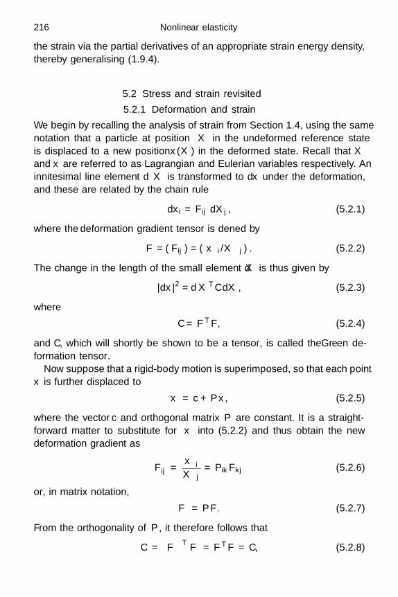
216 Nonlinear elasticity
the strain via the partial derivatives of an appropriate strain energy density,thereby generalising (1.9.4).
5.2 Stress and strain revisited
5.2.1 Deformation and strain
We begin by recalling the analysis of strain from Section 1.4, using the samenotation that a particle at position X in the undeformed reference stateis displaced to a new position x(X) in the deformed state. Recall that X
and x are referred to as Lagrangian and Eulerian variables respectively. Aninfinitesimal line element dX is transformed to dx under the deformation,and these are related by the chain rule
dxi = Fij dXj, (5.2.1)
where the deformation gradient tensor is defined by
F = (Fij) = (∂xi/∂Xj) . (5.2.2)
The change in the length of the small element dX is thus given by
|dx|2 = dXTC dX, (5.2.3)
where
C = FTF, (5.2.4)
and C, which will shortly be shown to be a tensor, is called the Green de-formation tensor.
Now suppose that a rigid-body motion is superimposed, so that each pointx is further displaced to
x′ = c + Px, (5.2.5)
where the vector c and orthogonal matrix P are constant. It is a straight-forward matter to substitute for x′ into (5.2.2) and thus obtain the newdeformation gradient as
F ′ij =
∂x′i
∂Xj= PikFkj (5.2.6)
or, in matrix notation,
F ′ = PF. (5.2.7)
From the orthogonality of P , it therefore follows that
C′ =(F ′)T F ′ = FTF = C, (5.2.8)

5.2 Stress and strain revisited 217
so that C, unlike F , is invariant under any superimposed rigid-body motionof the material.
On the other hand, suppose we perform a rigid-body motion on the mate-rial before applying the deformation. In other words we consider the trans-formation
X → x(X ′), where X ′ = c + QX, (5.2.9)
where the vector c and orthogonal matrix Q are constant. Now the chainrule gives
F ′ =
(∂xi
∂X ′j
)= FQT (5.2.10)
and the corresponding Green deformation tensor is thus
C′ =(F ′)T F ′ = QCQT. (5.2.11)
This demonstrates that C transforms as a tensor under transformations ofthe reference configuration.
To connect with Chapter 1, let us note that if the displacement from X tox is a rigid-body motion, then F is orthogonal and, hence, C is equal to theidentity matrix I. We are therefore led to define the strain tensor E = (Eij),where
E =12
(C − I) =12(FTF − I
). (5.2.12)
By construction, E is a symmetric tensor which is objective, by which wemean that it has the same definition after arbitrary rotation of the axes,and is zero for a rigid-body displacement. Also (5.2.3), written in the form(1.4.4), namely
|dx|2 − |dX|2 = 2dXTE dX, (5.2.13)
shows how the stretch of line elements in the continuum depends on E .We do not want the reader to drown under a deluge of new notations
in this introduction. Nonetheless, we note for future reference that anotherdeformation tensor can also be used, namely
B = FFT. (5.2.14)
This is called the left Green deformation tensor or, more commonly, theFinger tensor. We will find that B is more natural than C as a measure ofdeformation for an observer using Eulerian coordinates x.

218 Nonlinear elasticity
da
dx
n
dA
N
dX
Fig. 5.1 The deformation of a small scalene cylinder.
5.2.2 The Piola–Kirchhoff stress tensors
The elastic force exerted on a surface element da = n da in the deformedmedium, with area da and normal n, is given by
df = τn da, (5.2.15)
where τ = (τij) is the Cauchy stress tensor, as defined in Chapter 1. Asin Section 1.7, we will need to impose a constitutive relation between thestress and the strain tensor E , and this requires us to express τ relative toa Lagrangian frame.
As a first step, let us find how the surface element da is related to thearea dA that it occupied in the reference state. One way to do this is toconsider a small scalene cylinder in the reference state, with base dA andaxis dX. As shown in Figure 5.1, this will be deformed to a new cylinder,with base da and axis dx, which is related to dX by (5.2.1). The volumes ofthe two cylinders are given by dV = dX · dA and dv = dx · da respectivelyand, since the Jacobian J = det (()F ) measures the local volume change atany point, these must be related by dv = J dV . We therefore obtain
dx · da = dX ·(FTda
)= JdX · dA, (5.2.16)
in which the vector element dX is arbitrary, so the area elements are relatedby
da = det (F )(FT)−1
dA. (5.2.17)
When we apply this result to the expression (5.2.15) for the force on asmall area element, we obtain
df =
det (F ) τ(FT)−1
dA. (5.2.18)

5.2 Stress and strain revisited 219
This gives the stress in the deformed configuration on an area element which,in the reference configuration, was given by dA. The quantity in braces,
T = det (F )τ(FT)−1
, (5.2.19)
is a second-rank tensor called the first Piola–Kirchhoff stress tensor.As shown in Section 1.4, the Cauchy stress tensor τ is symmetric, but
T in general is not. We can, though, use the symmetry of τ to deduce thefollowing identity satisfied by T :
T FT = FT T. (5.2.20)
This motivates the introduction of the second Piola–Kirchhoff stresstensor S, defined by
S = F−1T = det (F ) F−1τ(FT)−1
, (5.2.21)
so that S is symmetric.
5.2.3 The momentum equation
In Section 1.6 we derived Cauchy’s momentum equation
ρ∂2xi
∂t2= ρgi +
∂τij
∂xj, (5.2.22)
which must apply to any continuum for which a Cauchy stress tensor (τij)can be defined. In (5.2.22), gi are the components of the applied body forceand ρ is the density of the material, related to the initial density ρ0 by
ρ0
ρ= J = det (F ). (5.2.23)
Now let us derive the Lagrangian equivalent of (5.2.22). We start, as inSection 1.6, by applying Newton’s second law to a material volume V (t)whose boundary ∂V (t) has outward unit normal denoted by n = (ni):
ddt
∫∫∫V (t)
∂xi
∂tρ dx =
∫∫∫V (t)
giρ dx +∫∫
∂V (t)τijnj da. (5.2.24)
Now we change the integration variables to Lagrangian coordinates X, using(5.2.17) to convert the final surface integral:
ddt
∫∫∫V (0)
∂xi
∂tρJ dX =
∫∫∫V (0)
giρJ dX +∫∫
∂V (0)
JτikF
−1jk
Nj dA.
(5.2.25)

220 Nonlinear elasticity
With respect to Lagrangian variables, the integration domain V (0) is time-independent, so we may differentiate through the first integral, using thefact that ρJ = ρ0(X) is independent of t. In the final integral, we recognisethe term in braces as the first Piola–Kirchhoff tensor Tij and apply thedivergence theorem to obtain∫∫∫
V (0)
∂2xi
∂t2ρ0 dX =
∫∫∫V (0)
giρ0 dX +∫∫∫
V (0)
∂Tij
∂XjdX. (5.2.26)
Since this must hold for all reference volumes V (0) we deduce, assumingthat the integrand is continuous, the following Lagrangian form of Cauchy’sequation:
ρ0∂2xi
∂t2= ρ0gi +
∂Tij
∂Xj. (5.2.27)
Although it is not immediately obvious, (5.2.27) may also be obtaineddirectly by using (5.2.19) to replace τ with T in (5.2.22) and applying thechain rule (Exercise 5.2).
5.2.4 Example: one-dimensional nonlinear elasticity
The simplest example that illustrates both mechanical and geometric non-linearity is a unidirectional displacement u(X, t) in the X-direction. In thisvery special situation, S and E just involve scalars Sxx and Exx and the mostgeneral constitutive law is simply a functional relationship between them,that is Sxx = φ (Exx). From (5.2.13), we obtain the one-dimensional strain
Exx =∂u
∂X+
12
(∂u
∂X
)2
(5.2.28)
and hence
Txx = (FS)xx =∂x
∂Xφ
(∂u
∂X+
12
(∂u
∂X
)2)
. (5.2.29)
In equilibrium under a constant stress Txx, the displacement is such that(1 +
∂u
∂X
)φ
(∂u
∂X+
12
(∂u
∂X
)2)
= Txx. (5.2.30)
If we suppose that the material is mechanically linear, so that φ is the linearfunction
φ (Exx) = (λ + 2µ) Exx, (5.2.31)
then (5.2.30) is a cubic equation for ∂u/∂X with only one real root.

5.3 The constitutive relation 221
More exciting possibilities occur when we examine longitudinal wavespropagating in the X-direction. Again assuming the linear constitutive re-lation (5.2.31), we find that the momentum equation (5.2.27) in one spatialdimension reads
∂2u
∂t2= c2
p
∂
∂X
[(1 +
∂u
∂X
)(1 +
12
∂u
∂X
)∂u
∂X
], (5.2.32)
where c2p = (λ + 2µ)/ρ0. This is a nonlinear generalisation of the P -wave
equation that we encountered in Chapter 3. We recall that one-dimensionallinear P -waves propagate information along the two families of characteris-tics X ± cpt = const. in the (X, t)-plane. However, for (5.2.32), the charac-teristics are given by the equation
dX
dt= ± cp
(1 + 3
∂u
∂X+
32
(∂u
∂X
)2)1/2
, (5.2.33)
and they are generally not straight lines. Even more importantly, they de-pend on the solution ∂u/∂X itself, and it can be shown that characteristicsof the same family will almost always eventually cross. When this happens,the pieces of information carried by each of these two characteristics areusually incompatible, so that u becomes multi-valued. This results in theformation of a shock, which is a curve in the (X, t)-plane across which thefirst derivatives of u are discontinuous (Bland, 1988, Section 10.1).
5.3 The constitutive relation
5.3.1 Polar decomposition
The polar decomposition theorem (Strang, 1988) tells us that any non-singular matrix F may be written as the product of an orthogonal matrixMT and a positive definite symmetric matrix U :
F = MTU. (5.3.1)
Hence, if the real, positive eigenvalues of U are denoted λ1, λ2 and λ3, thereexists an orthogonal matrix R such that
U = RTΛR, where Λ =
λ1 0 00 λ2 00 0 λ3
. (5.3.2)
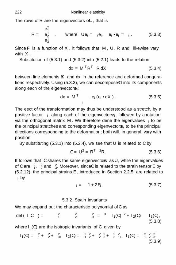
222 Nonlinear elasticity
The rows of R are the eigenvectors of U , that is
R =
eT1
eT2
eT3
, where Uei = λiei, ei · ej = δij . (5.3.3)
Since F is a function of X, it follows that M , U , R and Λ likewise varywith X.
Substitution of (5.3.1) and (5.3.2) into (5.2.1) leads to the relation
dx = MTRTΛR dX (5.3.4)
between line elements dX and dx in the reference and deformed configura-tions respectively. Using (5.3.3), we can decompose dX into its componentsalong each of the eigenvectors ei:
dx = MT∑
i
λi ei (ei · dX) . (5.3.5)
The effect of the transformation may thus be understood as a stretch, by apositive factor λi, along each of the eigenvectors ei, followed by a rotationvia the orthogonal matrix M . We therefore define the eigenvalues λi to bethe principal stretches and corresponding eigenvectors ei to be the principaldirections corresponding to the deformation; both will, in general, vary withposition.
By substituting (5.3.1) into (5.2.4), we see that U is related to C by
C = U2 = RTΛ2R. (5.3.6)
It follows that C shares the same eigenvectors ei as U , while the eigenvaluesof C are λ2
1, λ22 and λ2
3. Moreover, since C is related to the strain tensor E by(5.2.12), the principal strains Ei, introduced in Section 2.2.5, are related toλi by
λi =√
1 + 2Ei. (5.3.7)
5.3.2 Strain invariants
We may expand out the characteristic polynomial of C as
det (ζI − C) =(ζ − λ2
1) (
ζ − λ22) (
ζ − λ23)
= ζ3 − I1(C)ζ2 + I2(C)ζ − I3(C),(5.3.8)
where Ij(C) are the isotropic invariants of C, given by
I1(C) = λ21 + λ2
2 + λ23, I2(C) = λ2
1λ22 + λ2
2λ23 + λ2
3λ21, I3(C) = λ2
1λ22λ
23.
(5.3.9)
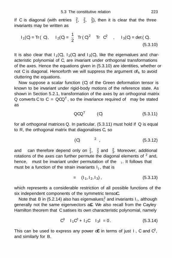
5.3 The constitutive relation 223
If C is diagonal (with entries λ21, λ2
2, λ23), then it is clear that the three
invariants may be written as
I1(C) = Tr (C), I2(C) =12
Tr (C)2 − Tr
(C2) , I3(C) = det (C).
(5.3.10)
It is also clear that I1(C), I2(C) and I3(C), like the eigenvalues and char-acteristic polynomial of C, are invariant under orthogonal transformationsof the axes. Hence the equations given in (5.3.10) are identities, whether ornot C is diagonal. Henceforth we will suppress the argument of Ik to avoidcluttering the equations.
Now suppose a scalar function φ(C) of the Green deformation tensor isknown to be invariant under rigid-body motions of the reference state. Asshown in Section 5.2.1, transformation of the axes by an orthogonal matrixQ converts C to C′ = QCQT, so the invariance required of φ may be statedas
φ(QCQT) ≡ φ (C) (5.3.11)
for all orthogonal matrices Q. In particular, (5.3.11) must hold if Q is equalto R, the orthogonal matrix that diagonalises C, so
φ (C) ≡ φ(Λ2) , (5.3.12)
and φ can therefore depend only on λ21, λ2
2 and λ23. Moreover, additional
rotations of the axes can further permute the diagonal elements of Λ2 and,hence, φ must be invariant under permutation of the λi. It follows that φ
must be a function of the strain invariants Ij , that is
φ = φ (I1, I2, I3) , (5.3.13)
which represents a considerable restriction of all possible functions of thesix independent components of the symmetric tensor C.
Note that B in (5.2.14) also has eigenvalues λ2i and invariants Ii, although
generally not the same eigenvectors as C. We also recall from the Cayley–Hamilton theorem that C satisfies its own characteristic polynomial, namely
C3 − I1C2 + I2C − I3I = 0. (5.3.14)
This can be used to express any power of C in terms of just I, C and C2,and similarly for B.

224 Nonlinear elasticity
5.3.3 Frame indifference and isotropy
Now we are at last in a position to relate stress and strain in the Lagrangianreference frame. A material is called elastic if the second Piola–Kirchhoffstress is a function only of the deformation gradient; that is,
S = S(F ); (5.3.15)
S could also depend on X if the elastic properties were spatially non-uniform, but we will ignore this possibility here.
The key requirement is that the relation (5.3.15) be invariant under rigid-body motions; in other words, the way a material responds to stress shouldnot depend on the frame in which it is observed. As demonstrated in Sec-tion 5.2.1, rotation of the Eulerian coordinate axes through an orthogonalmatrix P transforms F to F ′ = PF , so this frame indifference leads to therestriction
S (F ) ≡ S (PF ) (5.3.16)
for all orthogonal matrices P . Since the Green deformation tensor C is invari-ant under rigid-body motions, (5.3.16) is certainly satisfied if the constitutiverelation takes the form
S = S(C), (5.3.17)
and it may be shown, as in Exercise 5.3, that this condition is necessary aswell as sufficient. Notice that (5.3.17) is more specific than (5.3.15) since Chas only six distinct elements, while F has nine.
Further simplification may be achieved by assuming that the materialis isotropic, meaning it has no preferred directions. Suppose we take theundeformed material and rotate it about an arbitrary origin X0 via anorthogonal matrix Q such that
X ′ = X0 + Q (X − X0) . (5.3.18)
Then, if we take the rotated material and apply exactly the same deforma-tion as before, the net deformation is given by
X → x(X ′) = x(X0 + Q (X − X0)
). (5.3.19)
As shown in Section 5.2.1, the Green deformation tensor corresponding to(5.3.19) is C′ = QCQT, and the corresponding stress tensor at the point X0
is therefore
S ′ (C) = S(QCQT) . (5.3.20)

5.3 The constitutive relation 225
If the material is isotropic, then this should be identical to the stress whichwe would have obtained without the original rotation, albeit related to thenew coordinates X ′ rather than to X. By applying the usual rule for therotation of a tensor, we deduce that
S ′(C) = QS(C)QT, (5.3.21)
which must apply identically for any fixed point X0 and any rotationmatrix Q. The constitutive relation (5.3.17) between S and C must thereforesatisfy the symmetry condition
S(QCQT) ≡ QS(C)QT (5.3.22)
for all orthogonal matrices Q, at any point X at which the material isisotropic.
It may be shown (Exercise 5.4) that S has the symmetry property (5.3.22)if and only if it can be written in the form
S(C) = φ0 (I1, I2, I3) I + φ1 (I1, I2, I3) C + φ2 (I1, I2, I3) C2, (5.3.23)
where φ0, φ1 and φ2 are functions of the three invariants of C. An isotropicconstitutive relation thus amounts to a specification of these three scalarfunctions.
We note that, in the limit of small strain, when Cij → δij +2eij in the no-tation of Chapter 1, the only relevant strain invariant is the trace ekk . Hencethe right-hand side of (5.3.23) reduces to a linear combination of ekkδij fromthe first term and eij from the second and third terms, thereby retrieving(1.7.6). We will return to the small displacement limit in Section 5.3.6.
We may directly infer from (5.3.23) that in an isotropic material, S has thesame eigenvectors as C. On the other hand, using (5.2.19), equation (5.3.23)gives, for the Cauchy stress,
τ = I−1/23
[φ0B + φ1B2 + φ2B3] , (5.3.24)
so that the principal axes of τ coincide with those of B. Furthermore, us-ing (5.3.14), one can eliminate B3 and obtain
τ = I−1/23
[I3φ2I + (φ0 − I2φ2)B + (φ1 + I1φ2)B2] . (5.3.25)
This demonstrates how the Cauchy stress is more elegantly expressed interms of B, while C is more natural for the Piola–Kirchhoff stress.
If the material is not pre-stressed, then S should be zero in the referenceconfiguration, that is S(I) = 0, which leads to the condition
φ0(3, 3, 1) + φ1(3, 3, 1) + φ2(3, 3, 1) = 0. (5.3.26)

226 Nonlinear elasticity
However, we will see in the next section that the requirement (5.3.26) is farfrom sufficient for the constitutive relation (5.3.23) to lead to a physicallyacceptable theory of mechanically nonlinear elasticity.
5.3.4 The energy equation
In Chapter 1, we found that the work done on any region of a linear elasticsolid is balanced by the change in both the kinetic energy and the strainenergy stored by the material as it deforms. Now let us try to repeat thisanalysis for a nonlinear elastic material. We start by multiplying the momen-tum equation (5.2.27) by the velocity ∂xi/∂t and integrating over a controlmaterial volume V0:∫∫∫
V0
ρ0∂xi
∂t
∂2xi
∂t2dX =
∫∫∫V0
ρ0gi∂xi
∂tdX +
∫∫∫V0
∂xi
∂t
∂Tij
∂XjdX. (5.3.27)
The time derivative may be taken outside the first integral, while the finalintegral can be manipulated using the divergence theorem to obtain
ddt
∫∫∫V0
ρ0
2
(∂xi
∂t
)2
dX +∫∫∫
V0
Tij∂Fij
∂tdX
=∫∫∫
V0
ρ0gi∂xi
∂tdX +
∫∫∂V0
∂xi
∂tTijNj dA. (5.3.28)
Recalling that ρ0 dX ≡ ρ dx, we see that the first term on the left-hand sideof (5.3.28) is the rate of change of kinetic energy, while the first term on theright-hand side is the rate at which work is done by the body force. Finally,the boundary integral is the rate at which work is done by stress on ∂V .
We can therefore interpret the second term on the left-hand side of (5.3.28)as the rate at which elastic energy is stored by the medium. Unfortunately,this implies that apparently legitimate nonlinear constitutive relations mayallow a net extraction of energy from an elastic material under periodicloading cycles. Let us consider, for example, a material with the isotropicconstitutive relation
S =(λ2
1λ22λ
23 − 1
)I. (5.3.29)
subject to a deformation in which
F =
λ1 (t) 0 00 λ2 (t) 00 0 1
, (5.3.30)

5.3 The constitutive relation 227
where λ1, λ2 are periodic functions of t. We use (5.2.21) to calculate thefirst Piola–Kirchhoff stress as
T = FS =(λ2
1λ22 − 1
)λ1 (t) 0 00 λ2 (t) 00 0 1
(5.3.31)
and hence find that∫∫∫V0
Tij∂Fij
∂tdX = V0
(λ2
1λ22 − 1
)(λ1
dλ1
dt+ λ2
dλ2
dt
), (5.3.32)
which is a function whose time integral over a period may be positive ornegative. When λ1 = 1 + a cos(ωt), λ2 = 1 + b sin(ωt), for example, theintegral of (5.3.32) over a period 2π/ω is 3πab
(b2 − a2
)/2. Hence, if an
elastic material were to exist that satisfied (5.3.29), then it could be used asa limitless energy source!
This behaviour is clearly unacceptable and a sufficient condition to pre-clude it is the existence of a strain energy density W (Fij) such that
Tij =∂W∂Fij
, (5.3.33a)
or, introducing the convenient notation for differentiation by a tensor,
T =∂W∂F
. (5.3.33b)
If so, then we can write∫∫∫V0
Tij∂Fij
∂tdX ≡ d
dt
∫∫∫V0
W dX, (5.3.34)
and interpret the right-hand side as the strain energy stored in the medium;the change in this energy automatically integrates to zero over a periodicloading cycle. We will now explore this happy circumstance in more detail.
5.3.5 Hyperelasticity
A material is called hyperelastic if there is a strain energy density W (Fij)satisfying (5.3.33). The theory of hyperelasticity has proved to be by farthe most commonly-used and convenient way to construct constitutive re-lations for materials like rubber. By posing a functional form for W, andinferring from (5.3.33) the corresponding stress–strain relation, one auto-matically avoids thermodynamically unfeasible situations like that describedabove. However, the mere existence of W is not sufficient to guarantee well-posedness of the resulting elastic model. At the moment all we can say is
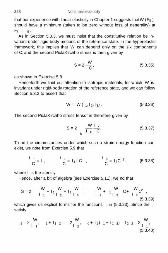
228 Nonlinear elasticity
that our experience with linear elasticity in Chapter 1 suggests that W (Fij)should have a minimum (taken to be zero without loss of generality) atFij = δij .
As in Section 5.3.3, we must insist that the constitutive relation be in-variant under rigid-body motions of the reference state. In the hyperelasticframework, this implies that W can depend only on the six componentsof C, and the second Piola–Kirchhoff stress is then given by
S = 2∂W∂C , (5.3.35)
as shown in Exercise 5.8.Henceforth we limit our attention to isotropic materials, for which W is
invariant under rigid-body rotation of the reference state, and we can followSection 5.3.2 to assert that
W = W (I1, I2, I3) . (5.3.36)
The second Piola–Kirchhoff stress tensor is therefore given by
S = 2∑
k
∂W∂Ik
∂Ik
∂C . (5.3.37)
To find the circumstances under which such a strain energy function canexist, we note from Exercise 5.9 that
∂I1
∂C = I,∂I2
∂C = I1I − C,∂I3
∂C = I3C−1, (5.3.38)
where I is the identity.Hence, after a bit of algebra (see Exercise 5.11), we find that
S = 2[(
∂W∂I1
+ I1∂W∂I2
+ I2∂W∂I3
)I −
(∂W∂I2
+ I1∂W∂I3
)C +
∂W∂I3
C2]
,
(5.3.39)which gives us explicit forms for the functions φi in (5.3.23). Since the φi
satisfy
φ2 = 2∂W∂I3
, φ1 + I1φ2 = −2∂W∂I2
, φ0 + I1 (φ1 + I1φ2) − I2φ2 = 2∂W∂I1
,
(5.3.40)

5.3 The constitutive relation 229
cross-differentiation reveals that
∂φ1
∂I3+
∂φ2
∂I2+ I1
∂φ2
∂I3= 0, (5.3.41a)
∂φ0
∂I3+ I1
∂φ1
∂I3+(I21 − I2
) ∂φ2
∂I3− ∂φ2
∂I1= 0, (5.3.41b)
∂φ0
∂I2+ I1
∂φ1
∂I2+
∂φ1
∂I1+(I21 − I2
) ∂φ2
∂I2+ I1
∂φ2
∂I1= 0. (5.3.41c)
Any choice of the functions φi that does not satisfy (5.3.41) will lead tobehaviour such as that exhibited in (5.3.32); indeed it was these integrabilityconditions that suggested the counter-example (5.3.29).
We note from (5.2.21) that the Cauchy stress is given in terms of W as
τ = I−1/23
∂W∂F
FT (5.3.42)
and, as shown in Exercise 5.7, this leads to the useful expression
τi = I−1/23 λi
∂W∂λi
(5.3.43)
(no summation) for the Cauchy principal stresses.As well as clarifying the characterisation of elastic materials, hyperelastic-
ity also often simplifies the mathematical and numerical analysis of nonlinearelastic problems. The net elastic energy stored in a material volume V0 isgiven by
U =∫∫∫
V0
W dX. (5.3.44)
By virtue of (5.3.33), a calculation analogous to Exercise 1.8 implies that thesteady version of the gravity-free momentum equation (5.2.27) is a necessarycondition for U to be minimised with respect to the displacement, assumingof course that W is sufficiently smooth. Crucially, the minimisation of afunctional like (5.3.44) is generally easier computationally than solving thenonlinear partial differential equation (5.2.27). In particular, minimisationproblems of this type are naturally suited to the finite element method (seeFung & Tong, 2001, Chapter 18).
However, for a nonlinear material, finding the uniqueness and smoothnessof a minimum of (5.3.44) now poses a typically difficult challenge in thecalculus of variations. It transpires that not only do we require W to bestrictly positive except at F = I, but also that it should be quasi-convex,which demands that the level surfaces of W are convex in a suitable functionspace. It is also difficult to compare this result with the condition that, in

230 Nonlinear elasticity
equilibrium, (5.2.27) should comprise, with suitable boundary conditions, awell-posed system for xi.
5.3.6 Linear elasticity
Now we briefly verify that the hyperelastic formulation of elasticity out-lined above reduces to the linear elastic constitutive relation introduced inChapter 1 when the strains are small. We recall from (5.3.7) that the prin-cipal strains are related to the principal stretches by
λi =√
1 + 2Ei ∼ 1 + Ei (5.3.45)
when |Ei| 1.Also we recall that W is a function of the principal stretches λ1, λ2, λ3
with a unique global minimum at λj ≡ 1. Moreover, for isotropic mate-rials, W is invariant under permutations of λ1, λ2, λ3. Hence, as λ1, λ2,
λ3 → 1, the local behaviour of W near its minimum must take the form
W ∼ µ3∑
i=1
(λi − 1)2 +λ
2
3∑i,j=1
(λi − 1) (λj − 1) , (5.3.46)
where the scalar constants λ and µ, which we will shortly identify with theLame constants of Chapter 1, must satisfy µ > 0 and 3λ+2µ > 0 for (5.3.46)to be positive definite.
Since, in principal axes, W = W(λi) and C = diag(λ2
i
), (5.3.35) implies
that
Si =1λi
∂W∂λi
. (5.3.47)
Substitution from (5.3.45) and (5.3.46) thus leads to
Si ∼ λ (λ1 + λ2 + λ3 − 3) + 2µ (λi − 1) ∼ λ (E1 + E2 + E3) + 2µEi (5.3.48)
as the strain tends to zero. The stress and strain tensors are thus related by
S ∼ λ Tr (E) I + 2µE , (5.3.49)
and, since the left- and right-hand sides both transform as tensors, (5.3.49)holds with respect to any chosen axes.
If the displacement is small, relative to any other length-scale, then thedeformation gradient F is approximately equal to the identity and hence,from (5.2.19) and (5.3.48), both the Piola–Kirchhoff stress tensors and theCauchy stress tensor are all approximately equal. In addition, the quadratic
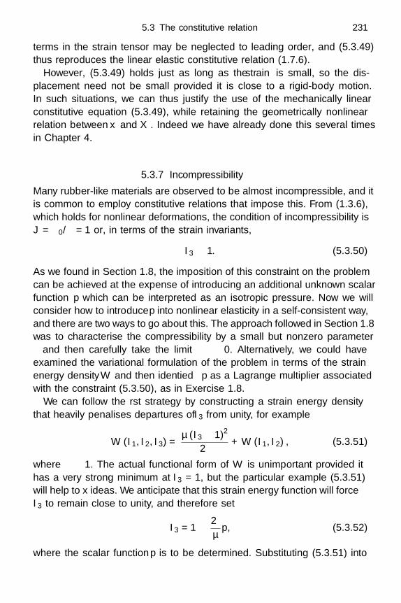
5.3 The constitutive relation 231
terms in the strain tensor may be neglected to leading order, and (5.3.49)thus reproduces the linear elastic constitutive relation (1.7.6).
However, (5.3.49) holds just as long as the strain is small, so the dis-placement need not be small provided it is close to a rigid-body motion.In such situations, we can thus justify the use of the mechanically linearconstitutive equation (5.3.49), while retaining the geometrically nonlinearrelation between x and X. Indeed we have already done this several timesin Chapter 4.
5.3.7 Incompressibility
Many rubber-like materials are observed to be almost incompressible, and itis common to employ constitutive relations that impose this. From (1.3.6),which holds for nonlinear deformations, the condition of incompressibility isJ = ρ0/ρ = 1 or, in terms of the strain invariants,
I3 ≡ 1. (5.3.50)
As we found in Section 1.8, the imposition of this constraint on the problemcan be achieved at the expense of introducing an additional unknown scalarfunction p which can be interpreted as an isotropic pressure. Now we willconsider how to introduce p into nonlinear elasticity in a self-consistent way,and there are two ways to go about this. The approach followed in Section 1.8was to characterise the compressibility by a small but nonzero parameterε and then carefully take the limit ε → 0. Alternatively, we could haveexamined the variational formulation of the problem in terms of the strainenergy density W and then identified p as a Lagrange multiplier associatedwith the constraint (5.3.50), as in Exercise 1.8.
We can follow the first strategy by constructing a strain energy densitythat heavily penalises departures of I3 from unity, for example
W (I1, I2, I3) =µ (I3 − 1)2
2ε+ W (I1, I2) , (5.3.51)
where ε 1. The actual functional form of W is unimportant provided ithas a very strong minimum at I3 = 1, but the particular example (5.3.51)will help to fix ideas. We anticipate that this strain energy function will forceI3 to remain close to unity, and therefore set
I3 = 1 − 2ε
µp, (5.3.52)
where the scalar function p is to be determined. Substituting (5.3.51) into

232 Nonlinear elasticity
(5.3.39) and using (5.3.14), we find that our desired constitutive relationbecomes
S = 2(
∂W∂I1
+ I1∂W∂I2
)I − 2
∂W∂I2
C − pC−1. (5.3.53)
The status of p as a hydrostatic pressure is clearer in the correspondingexpression for the Cauchy stress, namely
τ = −pI + 2(
∂W∂I1
+ I1∂W∂I2
)B − 2
∂W∂I2
B2. (5.3.54)
To arrive at the same conclusion from a purely variational viewpoint, wenote that incompressibility is satisfied in a small virtual displacement byadding to Fij an increment δFij such that
∂
∂Fij(det F ) δFij = 0. (5.3.55)
In Exercise 5.6, we show that this is equivalent to
F−1ji δFij = 0. (5.3.56)
We also note from (5.3.28) that no additional work is done by the incrementprovided
TijδFij = 0. (5.3.57)
Hence, considering only virtual deformations satisfying the constraint(5.3.56), we deduce that T is only determined up to an unknown scalarmultiple of
(FT
)−1. An arbitrary scalar multiple of C−1 may be thus addedto S, and (5.3.53) follows immediately.
5.3.8 Examples of constitutive relations
Some commonly used examples of constitutive relations for the strain energydensity are
neo-Hookean: W =µ
2(I1 − 3) , (5.3.58a)
Mooney–Rivlin: W = c1 (I1 − 3) + c2 (I2 − 3) , (5.3.58b)
Varga: W = 2µ (λ1 + λ2 + λ3 − 3) , (5.3.58c)
Ogden: W = 2µλα
1 + λα2 + λα
3 − 3α
, (5.3.58d)
where µ, c1, c2 and α are positive constants. In each case, the material is alsoassumed to be incompressible, so the constitutive relation is supplementedby the constraint I3 ≡ 1.
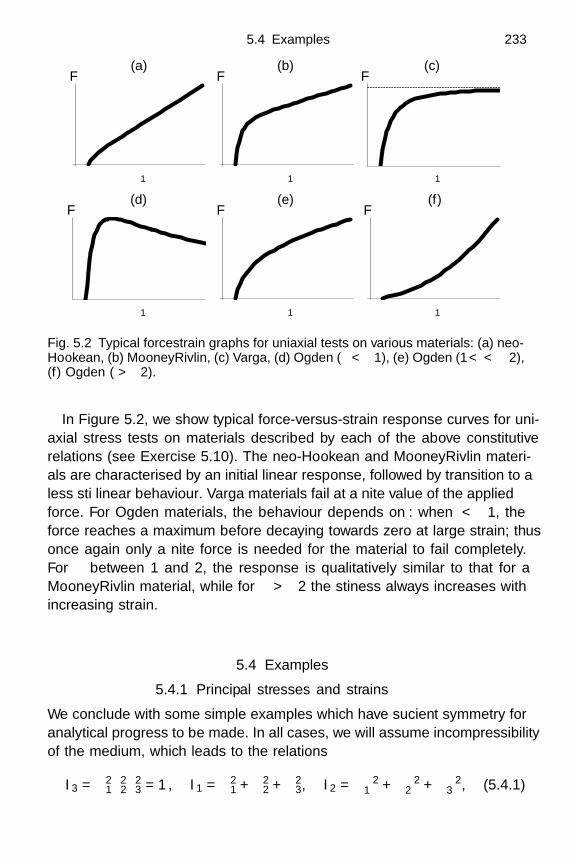
5.4 Examples 233
(d) (e) (f)
λ1
F F F
λ1 λ1
λ1 λ1
F F F
λ1
(a) (b) (c)
Fig. 5.2 Typical force–strain graphs for uniaxial tests on various materials: (a) neo-Hookean, (b) Mooney–Rivlin, (c) Varga, (d) Ogden (α < 1), (e) Ogden (1 < α < 2),(f) Ogden (α > 2).
In Figure 5.2, we show typical force-versus-strain response curves for uni-axial stress tests on materials described by each of the above constitutiverelations (see Exercise 5.10). The neo-Hookean and Mooney–Rivlin materi-als are characterised by an initial linear response, followed by transition to aless stiff linear behaviour. Varga materials fail at a finite value of the appliedforce. For Ogden materials, the behaviour depends on α: when α < 1, theforce reaches a maximum before decaying towards zero at large strain; thusonce again only a finite force is needed for the material to fail completely.For α between 1 and 2, the response is qualitatively similar to that for aMooney–Rivlin material, while for α > 2 the stiffness always increases withincreasing strain.
5.4 Examples
5.4.1 Principal stresses and strains
We conclude with some simple examples which have sufficient symmetry foranalytical progress to be made. In all cases, we will assume incompressibilityof the medium, which leads to the relations
I3 = λ21λ
22λ
23 = 1, I1 = λ2
1 + λ22 + λ2
3, I2 = λ−21 + λ−2
2 + λ−23 , (5.4.1)
234 Nonlinear elasticity
F
h
F
Fig. 5.3 A square membrane subject to an isotropic tensile force F .
for the strain invariants. In all the examples considered below, the stressand strain tensors are diagonal, and the principal stresses are found from(5.3.54) to be
τi = λi∂W∂λi
− p. (5.4.2)
Here, the λi are treated as independent variables while performing thederivatives. We focus on the Mooney–Rivlin constitutive relation (5.3.58b),for which (5.4.2) reads
τi = 2c1λ2i −
2c2
λ2i
− p, (5.4.3)
where we have made use of the incompressibility condition λ21λ
22λ
23 ≡ 1.
5.4.2 Biaxial loading of a square membrane
In this example, we consider a thin square membrane of initial thicknessh and side length loaded on its edges by a tensile force F , as shown inFigure 5.3. This leads to the uniform displacement field xi = λiXi, in whichcase the stresses are also uniform and given by (5.4.2). By relating these tothe applied force F , we obtain the equations
λ1∂W∂λ1
− p =F
λ2λ3h, λ2
∂W∂λ2
− p =F
λ1λ3h, λ3
∂W∂λ3
− p = 0, (5.4.4)
and elimination of p leads to
F
h=
∂W∂λ1
− λ3
λ1
∂W∂λ3
=∂W∂λ2
− λ3
λ2
∂W∂λ3
. (5.4.5)
To proceed further, we now have to choose a constitutive relation. Usingthe Mooney–Rivlin model (5.4.3), we find that the stretch ratios satisfy
(λ1 − λ2)[c1(1 + λ3
1λ32)
+ c2(λ2
1 + λ1λ2 + λ22 − λ4
1λ42)]
= 0. (5.4.6)

5.4 Examples 235
1 2 3 4 5
1
2
3
4
5
1 2 3 4 5
5
10
15
20
25
30
1 2 3 4 5
2.5
5
7.5
10
12.5
15
λ1 λ1 λ1
FWλ2
λc
(a) (b) (c)
Fig. 5.4 Response diagrams for a biaxially-loaded incompressible sheet of Mooney–Rivlin material with c2/c1 = 0.5. (a) Locus of compatible stretches with a symmet-ric square loading. (b) Strain energy density as a function of one of the stretches.(c) Applied force as a function of one of the stretches. The thin lines representa symmetric elastic response, the thick lines an asymmetric one, and the arrowsindicate the evolution of the stable solution as F increases.
This always has the solution λ1 = λ2 but, whenever c2 = 0, (5.4.6) alsoadmits asymmetric solutions in which λ1 = λ2. As shown in Figure 5.4(a),there is a critical value λc of the stretches at which symmetric responsebifurcates to an asymmetric one (see Exercise 5.12 for the details). We alsoshow in Figure 5.4(b) that, when λ1 > λc, the strain energy is reduced bybreaking the symmetry, so the asymmetric solution becomes energeticallyfavourable. Finally, in Figure 5.4(c), we show how the applied force varieswith the stretch. We see that as λ crosses λc, the stiffness of the sheetsuddenly reduces as it switches to an asymmetric response.
This example illustrates one of the most dramatic consequences of me-chanical nonlinearity: the strain response to a given load is generally notunique. We have already encountered non-uniqueness as the result of geo-metrical nonlinearity in Chapter 4 for the Euler strut, and we note that inboth cases the symmetry is broken in the bifurcation.
5.4.3 Blowing up a balloon
It is a common experience that blowing up a balloon is more difficult inthe early stages than it is later on. This phenomenon can be understoodby considering a thin, spherical, incompressible rubber membrane of initialradius R and thickness h R. Assuming the spherical symmetry is pre-served as the balloon inflates, the two tangential stretches λθ and λφ (whereθ and φ are the usual spherical polar coordinates) will be equal and related

236 Nonlinear elasticity
2 3 4 5 6
1
2
3
4
5
6
λθ
0
0.1
0.2c′ = 0.3P ′
Fig. 5.5 Scaled pressure inside a balloon as a function of the stretch λθ = R/r forvarious values of the Mooney–Rivlin parameter c′ = c2/c1 .
to the stretched radius r by
λθ = λφ =r
R, (5.4.7)
and the normal stretch λr is determined by incompressibility. Since the bal-loon is assumed to be thin, we can use the biaxial result above to calculatethe tension,
T = Tθ = Tφ = hλrτθ = hλr
(λθ
∂W∂λθ
− λr∂W∂λr
), (5.4.8)
noting that the thickness of the balloon is hλr following the deformation.The final observation is that a normal force balance relates the tension tothe internal pressure P and the curvature of the membrane via
P =2T
r. (5.4.9)
It is now a simple matter to assemble these ingredients and thus relatethe inflation pressure to the radius of the balloon. Again using the Mooney–Rivlin model (5.4.3), for example, we find
RP
hc1= P ′ (say) =
4(1 + c′λ2
θ
) (λ6
θ − 1)
λ7θ
, (5.4.10)
where c′ is the dimensionless ratio c2/c1.With c′ = 0, we see in Figure 5.5 that the pressure required to inflate the
balloon initially increases before decreasing when the radius is sufficientlylarge, successfully reproducing the familiar behaviour described above. Forsmall positive values of c′, however, the behaviour is more complicated, with
5.4 Examples 237
the pressure reaching a maximum, decreasing, then finally increasing againfor very large strains. In an experiment where a controlled pressure is im-posed (not generally possible using one’s lungs!), the radius would jumpas indicated by the arrow when the pressure reaches its maximum value.Increasing c′ corresponds to making the material stiffer at large strains, re-flecting the fact that polymer molecules can only withstand a finite extensionwithout breaking. If c′ exceeds a critical value(
11√
11 − 3425
)2/3
≈ 0.21446,
this increased stiffness removes the maximum in the pressure completely andthe behaviour becomes monotonic.
5.4.4 Cavitation
Suppose a spherical cavity embedded in a rubber continuum expands asa result of an increasing internal pressure P . Such a situation could beachieved by dissolving a gas in a rubber matrix, for example. Now we usespherical polar coordinates (R, θ, φ) in the rest state and again assume thedisplacement is purely radial, so that θ and φ are preserved while eachradial position R expands to a new radius r(R). We can hence write downthe principal stretches
λR =dr
dR, λφ = λθ =
r
R, (5.4.11)
and the incompressibility condition λRλθλφ = 1 gives us a differential equa-tion for r(R), namely
dr
dR=
R2
r2 . (5.4.12)
Denoting by a the initial radius of the sphere, we write the solution of(5.4.12) as
r =(R3 + λ3
0a3 − a3)1/3
, (5.4.13)
where
λ0 = λθ(0) =r(a)a
(5.4.14)
is the expansion ratio of the cavity. A displacement of the form (5.4.13) isthe only incompressible purely radial deformation. We can read off from

238 Nonlinear elasticity
2 3 4 5 6 7 8 9
2
4
6
8
10
λ0
c′ = 0
0.1
0.2P/c1
Fig. 5.6 Gas pressure inside a cavity as a function of inflation coefficient for variousvalues of the Mooney–Rivlin parameter c′ = c2/c1 .
(5.4.11) the principal stretches
λR =R2(
R3 + λ30a
3 − a3)2/3 , λφ = λθ =
(R3 + λ3
0a3 − a3
)1/3
R. (5.4.15)
We next turn to the familiar radial momentum equation from (1.11.16):
dτrr
dr+
2τrr − τθθ − τφφ
r= 0. (5.4.16)
We can use (5.4.13) to transform to Lagrangian coordinates and substitutefor the stress components from (5.4.2), thus obtaining
R3 + a3(λ2
0 − 1)
R2dτrr
dR= 2λθ
∂W∂λθ
− 2λR∂W∂λR
. (5.4.17)
Now solving the first-order differential equation (5.4.17) subject to the twoboundary conditions
τrr(a) = −P, τrr → 0 as R → ∞, (5.4.18)
yields an expression for the internal pressure P in terms of the inflationcoefficient λ0.
For Mooney–Rivlin materials, for example, this gives rise to the relation
P = c1
(5 − 4
λ0− 1
λ40
)− 2c2
(1 − 2λ0 +
1λ2
0
), (5.4.19)
which we plot in Figure 5.6 for various values of the ratio c2/c1. When c2 = 0,the material is neo-Hookean, and we see that only a finite pressure P = 5c1
is needed to inflate the cavity to infinity. This unlikely behaviour reflectsthe failure of the neo-Hookean model to capture the inability of materials

Exercises 239
to withstand unbounded strains, and the situation is remedied whenever c2
is positive.
5.5 Concluding remarks
This chapter has provided an introduction to what is probably the mostmathematically challenging branch of elasticity theory. In principle, our ba-sic task is to solve for xi from (5.2.27), bearing in mind that the stress isnow a much more complicated function of the strain than it was for me-chanically linear elasticity. Concerning the constitutive law, it is convenientto work with the second Piola–Kirchhoff tensor S, but there are now manymore physically acceptable relations between S and F than there were forlinear elasticity. Nonetheless, any selection of this relation must ultimatelylead to a well-posed system of partial differential equations for xi before wecan have confidence that we have a good model for the nonlinear evolutionof an elastic solid.
If we confine ourselves to statics, then it is conceptually appealing to workwith hyperelastic materials for which we have the apparently much simplertask of minimising the net strain energy (5.3.44). However, even here we haveto select from a wide range of functions relating the strain energy density tothe strain invariants, and, when we have done this, we still have to confrontthe daunting problem of the well-posedness of the relevant minimisationproblem in the calculus of variations.
Having at last faced up to the theoretical challenges of nonlinear elasticity,we are now in a position to discuss the implications for some of the practicallyimportant geometric configurations that we encountered in Chapter 4.
Exercises
5.1 Show that the displacement corresponding to a rigid-body motion isgiven by X(x, t) = a(t)+P (t)x, where the vector a and orthogonalmatrix P are spatially uniform. Show that the strain E defined by(5.2.12) is identically zero for this displacement field, but that thelinearised strain (1.7.1) is not.
5.2 (a) Prove the identity
∂
∂xj
(∂xj
∂Xk
)≡ 1
J
∂J
∂Xk, (E5.1)
(assuming the summation convention). [Hint: integrate both

240 Nonlinear elasticity
sides over an arbitrary material volume V (t) and use the di-vergence theorem.]
(b) Substitute the Piola–Kirchhoff stress tensor for the Cauchystress tensor in the momentum equation (5.2.22) and use thechain rule to obtain
ρ0∂2xi
∂t2= ρ0gi + JF−1
kj
∂
∂Xk
(J−1TilFjl
). (E5.2)
(c) Expand out the right-hand side of (E5.2) and apply the iden-tity (E5.1) to obtain the Lagrangian momentum equation(5.2.27).
5.3 Suppose the scalar function f of the two-dimensional matrix F isinvariant under the transformation F → PF , where P is any or-thogonal matrix. Let f(F ) = g(A, B, α, β), where F is written in theform
F =(
F11 F12
F21 F22
)=(
A cos α B cos β
A sinα B sinβ
).
By expressing P as the rotation matrix
P =(
cos θ sin θ
− sin θ cos θ
),
show that g must satisfy
g(A, B, α, β) ≡ g(A, B, α − θ, β − θ)
for all θ. Explain why g(A, B, α, β) ≡ h(A, B, α − β) for some func-tion h of three independent variables. Deduce that f = f(C), whereC = FTF .
[A conceptually equivalent argument works in three dimensions;see, for example, Noll (1958); Spencer (1970).]
5.4 (a) Suppose that two 2 × 2 symmetric matrices S and C satisfya functional relation S = S(C) which enjoys the symmetry(5.3.22) for all orthogonal matrices Q. By considering
Q =(
1 00 −1
),
or otherwise, show that S must be diagonal whenever C is.(b) With respect to coordinates in which C (and hence also S) is
diagonal, deduce that S must take the form
S =(
s1(λ21, λ
22) 0
0 s2(λ21, λ
22)
),
Exercises 241
where s1 and s2 are arbitrary functions of the eigenvalues λ21
and λ22 of C. Show that this expression may be manipulated
to
S = φ0(I1, I2)I + φ1(I1, I2)C, (E5.3)
where φ0 and φ1 are two arbitrary functions of the invariantsI1 and I2 of C (note that there are only two such invariantsin two dimensions).
(c) Show that (E5.3) is invariant with respect to orthogonal trans-formations and, hence, is true whether or not C is diagonal.
(d) Generalise the above argument to three dimensions.5.5 Considering only two-dimensional spatially linear displacements, with
(x1, x2) = (λ1(t)X1, λ2(t)X2) so that F and S are both diagonal,show that energy is consumed at a rate
q = λ1S11dλ1
dt+ λ2S22
dλ2
dt
per unit volume. Deduce that the medium conserves energy if andonly if the stress components satisfy
λ1∂S11
∂λ2≡ λ2
∂S22
∂λ1.
For the anisotropic constitutive relation
(S11,S22) = µ(λ2
1 + λ22)(1, α) ,
where α is a constant, show that, over a periodic cycle in which
λ1 = 1 + ε cos(ωt), λ2 = 1 + ε sin(ωt),
the net energy consumption per unit volume is∫ 2π/ω
0q dt = 2πε2(α − 1)µ.
5.6 Show that∂det (F )
∂Fij= det (F )F−1
ji .
[Hint: recall the inversion formula F−1ij = cofactor (Fji) / det(F ).]
5.7 Recall from Section 5.3.1 the existence of two orthogonal matricesR and M such that F = MTRTΛR, where Λ = diag (λi). Use thechain rule to show that
T =∂W∂F
= MTRT ∂W∂Λ
R.
242 Nonlinear elasticity
Now use the relationship (5.2.19) between the Cauchy and Piola–Kirchhoff stresses to show that
RMτMTRT = I−1/23
∂W∂Λ
Λ−1.
Since Λ is diagonal, deduce that the principal Cauchy stresses aregiven by (5.3.43).
5.8 If the strain energy density W is a function only of the symmetricGreen deformation tensor Cij , show that
∂W∂Fij
= Fik∂W∂Ckj
,
and deduce that the second Piola–Kirchhoff stress tensor is given by
S = 2∂W∂C .
5.9 Use Exercise 5.6 to prove the identities
(a)∂I1
∂Cij= δij , (b)
∂I2
∂Cij= I1δij − Cij , (c)
∂I3
∂Cij= I3C−1
ij .
5.10 Consider uniaxial stretching, in which a bar of initial cross-sectionalarea A is subject to an axial force F . Show that F is related to theaxial stretch λ1 by
F
A=
∂W∂λ1
− λ2
λ1
∂W∂λ2
,
where λ2 = λ3 = λ−1/21 . Hence justify the response diagrams shown
in Figure 5.2.5.11 Use the results from Exercise 5.9 to write out equation (5.3.37) as
S = 2[(
∂W∂I1
+ I1∂W∂I2
)I − ∂W
∂I2C + I3
∂W∂I3
C−1]
. (E5.4)
Using (5.3.14), deduce (5.3.39).5.12 Assuming the Mooney–Rivlin form for the strain energy in (5.4.4),
deduce (5.4.6). Show that the critical stretch λc, at which bifurcationfrom symmetric to asymmetric stretching occurs, is given implicitlyby
c2
c1= c′ =
1 + λ6c
λ2c (λ6
c − 3),
Exercises 243
where λc > 31/6. By introducing Θ = λ1λ2, show that the asymmet-ric solution satisfies
λ1 = λ±, λ2 =Θλ±
,
where
λ2± =
−P (Θ) ±√
P (Θ) + 4c′2Θ2
2c′, P (Θ) = 1 + Θ3 + c′
(Θ − Θ4) .
5.13 Consider a thin cylindrical tube, of initial radius R and thicknessh R, inflated by an internal air pressure P .
(a) Assuming the Mooney–Rivlin model and following the samemethodology as in Section 5.4.3, show that the internal pres-sure P and the axial tension Tz are related to the tangentialstretches by
P ′ =RP
hc1=
2(1 + c′λ2
z
) (λ4
θλ2z − 1
)λ4
θλ3z
,
Tz
hc1=
2(1 + c′λ2
θ
) (λ2
θλ4z − 1
)λ3
θλ3z
,
where c′ = c2/c1.(b) If the tube is constrained in the z-direction so that λz = 1,
show that only a finite pressure P ′ = 2 (1 + c′) is needed toinflate the tube to infinity. Show also that the axial tensionneeded to maintain zero displacement in the z-direction tendsto infinity as λθ does.
(c) Now, instead suppose that the tube is free to contract in thez-direction, so that Tz = 0. Show that in this case P ′ → ∞as λθ → ∞, although the behaviour is non-monotonic if
c′ >
(34 + 11
√11
7
)2/3
≈ 4.663.
5.14 (a) By changing independent variables to λθ , show that the dif-ferential equation (5.4.17) for the stress outside a sphericalcavity may be written in the form
−λθ
(λ3
θ − 1) dτrr
dλθ= 2λθ
∂W∂λθ
− 2λR∂W∂λR

244 Nonlinear elasticity
and, for the Mooney–Rivlin model, derive the equation
dτrr
dλθ= −
4(c1 + c2λ
2θ
) (λ3 + 1
)λ5
θ
.
(b) For a spherical cavity in an infinite medium, show that theappropriate boundary conditions are
τrr = −P at λθ = λ0, τrr → 0 as λθ → 1,
and hence obtain the relation (5.4.19) between the internalpressure P and the inflation parameter λ0.
(c) For a sphere with initial internal radius a and finite thicknessh, show that
P = c1
(4λ
+1λ4
− 4λ0
− 1λ4
0
)−2c2
(2λ −
1λ2
− 2λ0 +1λ2
0
),
where
λ =
(1 +
(λ3
0 − 1)a3
(a + h)3
)1/3
.
Hence recover the balloon result (5.4.10) in the limit h/a → 0.
6
Asymptotic analysis
6.1 Introduction
In Chapter 4, we derived various approximate models for thin or slenderelastic configurations such as rods and plates. These models were obtainedusing net force and moment balances combined with ad hoc constitutiverelations, for example between the bending moments and the curvatures.In this chapter, we show how such models may be derived systematicallyfrom the underlying continuum equations and boundary conditions. Weconcentrate on a few canonical models for plates, beams, rods and shells.Each of these models is important in its own right, and their derivationillustrates the tools that are widely useful for analysing more general thinstructures.
The basic idea is to exploit the slenderness of the geometry so as to sim-plify the equations of elasticity asymptotically. This process is made system-atic by first non-dimensionalising the equations, so that all the variables aredimensionless and of order one. This highlights the small slenderness param-eter ε = h/L, where h is a typical thickness and L a typical length of theelastic body. A simplified system of equations is then obtained by carefullytaking the limit ε → 0. Typically, the solution is sought as an asymptoticexpansion in powers of the small parameter ε, and the techniques demon-strated here fall within the general theories of asymptotic expansions andperturbation methods. Kevorkian & Cole (1981), Hinch (1991) and Bender& Orszag (1978) provide very good general expositions of these methods.
In fact we have already encountered an example of this approach whendiscussing the torsion of a thin-walled tube in Section 2.5, and an even sim-pler paradigm is the dimensionless model for antiplane strain of a thin plate.We will use this example in Section 6.2 to introduce the asymptotic argu-ments that form the basis of this chapter. Their systematic nature offers
245

246 Asymptotic analysis
many advantages compared to the less rigorous derivations of Chapter 4.For example, in principle the process allows further corrections to be cal-culated, resulting in increasingly accurate models. Furthermore, it makesexplicit the assumptions behind a simplified model, thus allowing us to esti-mate the error incurred in making an approximation and to determine whenthat approximation may become invalid. In this regard, we recall that thebeam and plate theories developed in Chapter 4 are unable to resolve thedetails of the tractions applied to the edges. A boundary layer analysis in theneighbourhood of these edges will allow us to explain how such tractions caneffectively be replaced by an equivalent point force/moment system, withouthaving to assume Saint-Venant’s principle. Finally, since we start from thegeneral continuum equations of elasticity, our asymptotic approach will leadto explicit formulae for practically useful parameters, such as the bendingstiffness, in terms of the underlying elastic parameters, such as the Lameconstants.
In Section 6.3 we re-derive the linear plate equation. As it describes in-finitesimal transverse displacements of a plate, we can obtain it startingfrom linear elasticity. In Section 6.4, we analyse a boundary layer near anedge of the plate and re-establish the correct boundary conditions for thismodel. Next, in Section 6.5, we re-derive the improved von Karman plateequations, incorporating geometrically nonlinear terms. This requires us tostart from the equations of nonlinear elasticity, although the asymptotic ap-proach is otherwise analogous to that used in Section 6.3. In Section 6.6,we extend the analysis to describe large two-dimensional deflections of aplate and thus derive the Euler strut equation. Finally, in Sections 6.7–6.8,we illustrate the geometrical generalisations needed to obtain the equationsgoverning infinitesimal displacements of rods and shells.
6.2 Antiplane strain in a thin plate
We first introduce our asymptotic methodology by modelling small antiplanedisplacements in a thin plate such that the region D in Figure 2.5 is therectangle 0 < y < h, 0 < x < L. The slenderness parameter in this case is
ε =h
L. (6.2.1)
Suppose the lateral boundaries of this plate are traction-free and that w
is prescribed on the ends x = 0, L. The first step towards an asymptoticanalysis is to non-dimensionalise the spatial coordinates and w by writing
x = Lx′, y = hy′, w = Ww′, (6.2.2)
6.2 Antiplane strain in a thin plate 247
where W is a typical displacement at the boundary. From (2.3.2) and (2.3.3)we find that the dimensionless displacement w′ satisfies
ε2 ∂2w′
∂x′2 +∂2w′
∂y′2= 0 with
∂w′
∂y′= 0 on y′ = 0, 1, (6.2.3)
along with w′ = f(y′) at x′ = 0 and w′ = g(y′) at x = 1, where both f and g
are prescribed functions. To avoid clutter in the equations, we drop theprimes henceforth.
Away from the ends of the plate, we expand w in an asymptotic expansionin which w ∼ w0 + ε2w2 + · · · as ε → 0. This gives, to lowest order in ε,
∂2w0
∂y2 = 0 with∂w0
∂y= 0 on y = 0, 1. (6.2.4)
Hence w0 = w0(x), but this function is not determined at this stage andwe must proceed further in the asymptotic expansion. Collecting all O
(ε2)
terms, we find that
∂2w2
∂y2 = −d2w0
dx2 with∂w2
∂y= 0 on y = 0, 1. (6.2.5)
The solution w2 can only satisfy both boundary conditions if∫ 1
0
∂2w2
∂y2 dy =[∂w2
∂y
]1
0. (6.2.6)
This solvability condition for w2 gives rise to the “thin sheet” equation
d2w0
dx2 = 0 (6.2.7)
for w0.To complete the model, we need to derive boundary conditions for (6.2.7).
We do this by subjecting the ends of the plate to a mathematical magnifyingglass. We first focus on the end x = 0 by setting x = εx and letting thedisplacement in this boundary layer near the edge be given by the function
w(x, y) = w(x, y). (6.2.8)
This gives the semi-infinite strip model
∂2w
∂x2 +∂2w
∂y2 = 0 with∂w
∂y= 0 on y = 0, 1 (6.2.9)
and w = f(y) prescribed on x = 0. Letting now w ∼ w0 + εw1 + · · · , using

248 Asymptotic analysis
separation of variables and making the assumption that w0 does not growas x → ∞, we find
w0 =a0
2+
∞∑n=1
ane−nπx cos nπy, (6.2.10)
where the ai are the Fourier cosine coefficients of f(y).Finally, we require that the functions w0 and w0 match, in the sense that,
as x → 0, w0 joins smoothly with w0 when the latter is evaluated for large x.More specifically, we require that
limx→0
w0 = limx→∞
w0, (6.2.11)
and we thus obtain
w0(0) =∫ 1
0f(y) dy, (6.2.12)
and similarly
w0(1) =∫ 1
0g(y) dy. (6.2.13)
These are the crucial boundary conditions for the thin sheet model (6.2.7):the only information that w0 has about f and g is their average values.
Now we undertake the more challenging task of extending this asymptoticargument to the bending of elastic plates.
6.3 The linear plate equation
6.3.1 Non-dimensionalisation and scaling
We now turn to small displacements in a horizontal elastic plate subject to atransverse gravitational acceleration g. As for the antiplane strain problemjust analysed, we assume that the displacements are small enough for linearelasticity to apply, so we can use the momentum equation given in compo-nent form by (1.11.3), and the components of the Cauchy stress tensor aregiven by (1.11.1). If the plate has uniform thickness h and its centre-surfaceinitially occupies the plane z = 0, then its free surfaces are at z = ±h/2,and we impose the stress-free boundary conditions
τxz = τyz = τzz = 0 on z = ±h/2. (6.3.1)
In linear elasticity we do not distinguish between Eulerian and Lagrangiancoordinates, so the boundaries of the plate effectively remain fixed at
6.3 The linear plate equation 249
z = ±h/2. The treatment of larger transverse displacements, comparableto h, say, will be deferred to Section 6.5.
Denoting by L a typical dimension in the x- and y-directions, the slender-ness parameter is again ε = h/L, and we will now construct an approximatetheory for the deformations of the plate based on the assumption that ε issmall. To exploit this fact, we again non-dimensionalise the equations beforetaking the asymptotic limit ε → 0, making the important assumption thatλ and µ are held fixed.
The spatial coordinates are again scaled with their typical values as
x = Lx′, y = Ly′, z = hz′. (6.3.2)
As always happens in asymptotic simplifications, choosing the right scalingsfor the dependent variables is a matter of trial-and-error guided by experi-ence. Here, simple geometry implies that a transverse displacement of magni-tude O (W ) is associated with in-plane displacements of O (εW ). Moreover,from (6.3.1), we know that, on the free surface, ∂u/∂z = −∂w/∂x. Now,we have the order-of-magnitude estimates ∂u/∂z ∼ u/h and ∂w/∂x ∼ w/L,and balancing the two yields the non-dimensionalisation
u = εWu′, v = εWv′, w = Ww′. (6.3.3)
The appropriate non-dimensionalisation for the stress components isslightly less clear. Our best strategy is to seek a scaling that balances asmany terms as possible in the Navier equations (1.11.3), and we give our-selves the freedom to do this by writing
(τxx, τxy, τyy) = τ
(τ ′xx, τ ′
xy, τ′yy
), (6.3.4a)
(τxz, τyz) = ετ
(τ ′xz, τyz
), (6.3.4b)
τzz = ε2ττ′zz , (6.3.4c)
where τ is to be determined. A suitable choice may then be obtained by bal-ancing the in-plane stresses and strains in the constitutive relation (1.11.1),which leads to
τ =ε2EW
h, (6.3.5)
where E is Young’s modulus. Finally, by looking for a balance in the

250 Asymptotic analysis
transverse Navier equation (1.11.3c), we infer a suitable time-scale, namely
t =(
h
ε2
√ρ
E
)t′. (6.3.6)
To summarise, the geometry of the plate has driven our non-dimensiona-lisation (6.3.2) of the spatial variables. Our scalings (6.3.3) of the displace-ments amount to assumptions about how big the transverse and in-planedeflections are; thereafter, stress components are rescaled so as to balanceas many terms as possible in the momentum equations. We will now derivethe leading-order model that results from these scalings.
6.3.2 Dimensionless equations
Substituting (6.3.2) and (6.3.4) into (1.11.3) and neglecting terms of orderε2 we obtain the dimensionless momentum equations
0 =∂τxx
∂x+
∂τxy
∂y+
∂τxz
∂z, (6.3.7a)
0 =∂τxy
∂x+
∂τyy
∂y+
∂τyz
∂z, (6.3.7b)
∂2w
∂t2=
∂τxz
∂x+
∂τyz
∂y+
∂τzz
∂z− G, (6.3.7c)
where
G =ρgh2
ε4EW(6.3.8)
is a dimensionless constant measuring the importance of gravity. Here, andhenceforth, we drop the primes to avoid cluttering the equations. The stress-free conditions (6.3.1) on the upper and lower surfaces simply become
τxz = τyz = τzz = 0 on z = ±1/2. (6.3.9)
It is helpful to average the momentum equations by integrating (6.3.7)with respect to z and applying (6.3.9). This yields
0 =∂Txx
∂x+
∂Txy
∂y, 0 =
∂Txy
∂x+
∂Tyy
∂y(6.3.10a)
and
∂2w
∂t2=
∂Nx
∂x+
∂Ny
∂y− G, (6.3.10b)

6.3 The linear plate equation 251
where w denotes the average of w across the plate, and the net in-plane andtransverse stresses are defined as in Section 4.6 by
Tij =∫ 1/2
−1/2τij dz, Nj =
∫ 1/2
−1/2τjz dz. (6.3.11)
Similarly, multiplication through by z before integrating leads to the momentbalance equations
0 =∂Myx
∂x+
∂Myy
∂y− Nx, 0 =
∂Mxx
∂x+
∂Mxy
∂y+ Ny, (6.3.12)
where the bending moments are defined as in Section 4.6 by
Myx =∫ 1/2
−1/2zτxx dz, Mxy = −
∫ 1/2
−1/2zτyy dz, (6.3.13a)
Myy = −Mxx =∫ 1/2
−1/2zτxy dz. (6.3.13b)
We may now use (6.3.12) to eliminate Nx and Ny from (6.3.10b) to give
∂2w
∂t2=
∂2Myx
∂x2 +∂2
∂x∂y(Myy − Mxx) − ∂2Mxy
∂y2 − G. (6.3.14)
Hence the deformation of the plate is governed by the averaged equa-tions (6.3.10a) and (6.3.14). We must now relate the averaged stresses andmoments to the displacements by using the dimensionless constitutive equa-tions. These take the form
ε2τxx =ε2(1 − ν)ux + ε2νvy + νwz
(1 + ν)(1 − 2ν), (6.3.15a)
τxy =uy + vx
2(1 + ν), (6.3.15b)
ε2τyy =ε2νux + ε2(1 − ν)vy + νwz
(1 + ν)(1 − 2ν), (6.3.15c)
ε2τxz =uz + wx
2(1 + ν), (6.3.15d)
ε2τyz =vz + wy
2(1 + ν), (6.3.15e)
ε4τzz =ε2νux + ε2νvy + (1 − ν)wz
(1 + ν)(1 − 2ν), (6.3.15f)
where ν is Poisson’s ratio and, in this chapter only, we will occasionally usesubscripts as shorthand for partial derivatives of the displacements. Whenwe take the limit ε → 0 in (6.3.15), we treat all the other parameters as

252 Asymptotic analysis
being O (1). In particular, we assume that ν is not too close to either −1 or1/2, so that we preclude situations such as that described in Section 1.8.
6.3.3 Leading-order equations
If we immediately set ε = 0 in (6.3.15), we get the same equation wz = 0three times. It is therefore expedient first to eliminate wz between the equa-tions to obtain
τxx − ε2ν
1 − ντzz =
ux + νvy
1 − ν2 , τyy −ε2ν
1 − ντzz =
νux + vy
1 − ν2 . (6.3.16)
This allows us simply to let ε tend to zero in the above equations withouthaving to write the dependent variables as explicit asymptotic expansions.
With w independent of z (to leading order), we may integrate (6.3.15d)and (6.3.15e) to obtain
u(x, y, z, t) = u(x, y, t) − zwx(x, y, t), (6.3.17a)
v(x, y, z, t) = v(x, y, t) − zwy(x, y, t) (6.3.17b)
as ε → 0. The first terms on the right-hand sides give purely in-plane dis-placements, while the terms proportional to z correspond to bending of theplate.
By substituting (6.3.17) back into (6.3.15) and integrating, we find thatthe averaged stresses and moments satisfy
Txx =ux + νvy
1 − ν2 , Txy =uy + vx
2(1 + ν), Tyy =
νux + vy
1 − ν2 , (6.3.18)
Myx = −wxx + νwyy
12(1 − ν2), Mxy =
νwxx + wyy
12(1 − ν2), (6.3.19a)
Myy = −Mxx = − wxy
12(1 + ν). (6.3.19b)
We are reassured by the fact that the expressions (6.3.18) for the in-planetensions agree with the exact biaxial straining solutions (2.2.19). Equally, therelations between the bending moments and the second derivativesof w reproduce those found in (4.6.8) by ad hoc comparison with exactplane stress solutions.
Recalling that Txx, Txy and Tyy satisfy (6.3.10a), we see that the in-planedisplacements satisfy a plane strain problem. As explained in Section 2.6,one approach to this problem is to introduce an Airy stress function A(x, y)

6.4 Boundary conditions and Saint-Venant’s principle 253
such that
Txx =∂2A
∂y2 , Txy = − ∂2A
∂x∂y, Tyy =
∂2A
∂x2 , (6.3.20)
and elimination of u and v shows that A satisfies the biharmonic equation
∇4A = 0. (6.3.21)
Also, by substituting (6.3.19) into (6.3.14), we find that the transverse dis-placement w satisfies the linear plate equation
wtt = − ∇4w
12(1 − ν2)− G. (6.3.22)
Notice that the equation (6.3.22) for w can be solved independently of u
and v. In other words, transverse bending completely decouples from in-plane deformation of the plate.
In summary, our model consists of the linear partial differential equation(6.3.22) for w and a decoupled biharmonic equation for A. We have derivedthese equations systematically, without invoking any other assumptions thanthe scalings in Section 6.3.1. Our derivation is constructive and yields explicitformulae for the other quantities of interest, that is the displacements andstress components.
Equation (6.3.22) does not contain the “membrane” term T∇2w obtainedfrom a momentum balance argument in Section 4.6. Since the tension T isproportional to the plane strain components ux, vy , etc., this product of T
with ∇2w is nonlinear in the displacements. As hinted at in Section 4.6, itis impossible, starting from the linear Navier equations (1.11.3) and consti-tutive relations (1.11.1), to obtain any such nonlinear terms. We will showbelow in Section 6.5 how they arise from a geometrically nonlinear model.
6.4 Boundary conditions and Saint-Venant’s principle
6.4.1 Boundary layer scalings
We are now poised to resolve systematically the difficulties encountered inSection 4.6.2 concerning the boundary conditions for plate models. In thelight of Section 6.2, it will come as no surprise that we must proceed by ad-dressing a boundary layer region near the edge of the plate. In this boundarylayer we will find a model that is fully three-dimensional, but fortunatelywe will not need to solve it in detail to obtain the sought-after boundaryconditions.
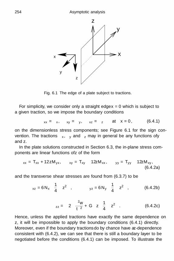
254 Asymptotic analysis
σx
σz
σy
z
x
y
Fig. 6.1 The edge of a plate subject to tractions.
For simplicity, we consider only a straight edge x = 0 which is subject toa given traction, so we impose the boundary conditions
τxx = σx, τxy = σy, τxz = σz at x = 0, (6.4.1)
on the dimensionless stress components; see Figure 6.1 for the sign con-vention. The tractions σx, σy and σz may in general be any functions of y
and z.In the plate solutions constructed in Section 6.3, the in-plane stress com-
ponents are linear functions of z of the form
τxx = Txx + 12zMyx, τxy = Txy − 12zMxx, τyy = Tyy − 12zMxy,
(6.4.2a)
and the transverse shear stresses are found from (6.3.7) to be
τxz = 6Nx
(14− z2
), τyz = 6Ny
(14− z2
), (6.4.2b)
τzz = −2(
∂2w
∂t2+ G
)z
(14− z2
). (6.4.2c)
Hence, unless the applied tractions have exactly the same dependence onz, it will be impossible to apply the boundary conditions (6.4.1) directly.Moreover, even if the boundary tractions do by chance have a z-dependenceconsistent with (6.4.2), we can see that there is still a boundary layer to benegotiated before the conditions (6.4.1) can be imposed. To illustrate the

6.4 Boundary conditions and Saint-Venant’s principle 255
difficulty, consider a traction-free edge, so that σx = σy = σz = 0. By naivelyapplying (6.4.1) to (6.4.2), we apparently obtain five conditions, namely
Txx = Txy = Myx = Mxx = Nx = 0. (6.4.3)
However, only four boundary conditions can be imposed on our model forthe plate, so at least one of these must be neglected.
To address this issue, as in Section 6.2 we now focus our attention on athin boundary layer in which x = εx, where x is O (1). To get a nontrivialbalance in the Navier equations (6.3.7), we also find it necessary to rescalesome of the stress components as follows:
τxz =τxz
ε, τyz =
τyz
ε, τzz =
τzz
ε2 . (6.4.4)
In view of (6.3.4), all stress components are now of the same order of mag-nitude. In particular, the transverse stress is two orders of magnitude largernear the edge of the plate than it is in the interior. This gives us a strongclue that the boundary layer may have an unexpected influence on the restof the plate.
6.4.2 Equations and boundary conditions
After we apply the rescaling (6.4.4) and neglect terms of order ε2, the Navierequations become
0 =∂τxx
∂x+ ε
∂τxy
∂y+
∂τxz
∂z, (6.4.5a)
0 =∂τxy
∂x+ ε
∂τyy
∂y+
∂τyz
∂z, (6.4.5b)
0 =∂τxz
∂x+ ε
∂τyz
∂y+
∂τzz
∂z. (6.4.5c)
Here we have used hats to distinguish dependent variables (even unscaledones) evaluated in the boundary layer from those in the interior. As ε → 0,(6.4.5) effectively reduces to a set of partial differential equations with onlyx and z as dependent variables, y being simply a parameter. The boundaryconditions on the edge and the upper and lower surfaces read
τxz = τyz = τzz = 0 on z = ±1/2, (6.4.6a)
τxx = σx, τxy = σy, τxz = εσz on x = 0. (6.4.6b)

256 Asymptotic analysis
The rescaled constitutive relations (6.3.15) take the form
ε2(1 + ν)(1 − 2ν)τxx = ε(1 − ν)∂u
∂x+ ε2ν
∂v
∂y+ ν
∂w
∂z, (6.4.7a)
2ε(1 + ν)τxy = ε∂u
∂y+
∂v
∂x, (6.4.7b)
ε2(1 + ν)(1 − 2ν)τyy = εν∂u
∂x+ ε2(1 − ν)
∂v
∂y+ ν
∂w
∂z, (6.4.7c)
2ε2(1 + ν)τxz = ε∂u
∂z+
∂w
∂x, (6.4.7d)
2ε(1 + ν)τyz =∂v
∂z+
∂w
∂y, (6.4.7e)
ε2(1 + ν)(1 − 2ν)τzz = εν∂u
∂x+ ε2ν
∂v
∂y+ (1 − ν)
∂w
∂z. (6.4.7f)
As in the antiplane strain example of Section 6.2, we must match the twosolutions: the asymptotic behaviour of the inner solution as x → ∞ must bethe same as that of the outer solution as x → 0. In other words, we imposethat
u ∼u(0, y) − z∂w
∂x(0, y) + εx
(∂u
∂x(0, y) − z
∂2w
∂x2 (0, y))
+ · · · , (6.4.8a)
v ∼ v(0, y) − z∂w
∂y(0, y) + εx
(∂v
∂x(0, y) − z
∂2w
∂x∂y(0, y)
)+ · · · , (6.4.8b)
w ∼w(0, y) + εx∂w
∂x(0, y) + · · · , (6.4.8c)
τxx ∼Txx(0, y) + 12zMyx(0, y) + · · · , (6.4.8d)
τxy ∼Txy(0, y) − 12zMxx(0, y) + · · · , (6.4.8e)
τxz ∼ 6εNx(0, y)(
14− z2
)+ · · · , (6.4.8f)
τyz ∼ 6εNy(0, y)(
14− z2
)+ · · · , (6.4.8g)
τzz ∼O(ε2) (6.4.8h)
as x → ∞.
6.4 Boundary conditions and Saint-Venant’s principle 257
6.4.3 Asymptotic expansions
Unlike the situation encountered in Section 6.3.3, there is now no way toavoid writing the dependent variables in asymptotic expansions in powersof ε, for example
τxx ∼ τ (0)xx + ετ (1)
xx + ε2 τ (2)xx + · · · . (6.4.9)
To leading order in ε, (6.4.5) becomes
0 =∂τ
(0)xx
∂x+
∂τ(0)xz
∂z, 0 =
∂τ(0)xy
∂x+
∂τ(0)yz
∂z, 0 =
∂τ(0)xz
∂x+
∂τ(0)zz
∂z, (6.4.10)
and the integrated versions of these equations are, simply,
0 =∂
∂x
∫ 1/2
−1/2τ (0)xx dz =
∂
∂x
∫ 1/2
−1/2τ (0)xy dz =
∂
∂x
∫ 1/2
−1/2τ (0)xz dz. (6.4.11)
Hence the average leading-order stresses are constant over the entire bound-ary layer and, in view of (6.4.6), (6.4.8d), and (6.4.8e), we immediatelydeduce that the two boundary conditions to be applied to (6.3.21) are
Txx(0, y) =∫ 1/2
−1/2σx(y, z) dz, (6.4.12a)
Txy(0, y) =∫ 1/2
−1/2σy(y, z) dz. (6.4.12b)
In the same way, multiplying (6.4.10a) by z and averaging over the thicknessof the plate, we obtain
0 =∂
∂x
∫ 1/2
−1/2zτ (0)
xx dz (6.4.13)
and therefore, combining (6.4.6) with (6.4.8d),
Myx(0, y) =∫ 1/2
−1/2zσx(y, z) dz. (6.4.14)
Equations (6.4.12) and (6.4.14) show that the net in-plane tractions andtheir moment along the edges are balanced by the corresponding stresses onthe other side of the boundary layer, as we might have expected physically.Equation (6.4.14), together with (6.3.19a), provides one boundary conditionfor the outer plate equation (6.3.22). One further boundary condition isneeded, and to obtain it we must proceed to the next order in ε, where(6.4.5c) yields
0 =∂τ
(1)xz
∂x+
∂τ(0)yz
∂y+
∂τ(1)zz
∂z. (6.4.15)

258 Asymptotic analysis
Integrating with respect to z, we now find that
0 =∂
∂x
∫ 1/2
−1/2τ (1)xz dz +
∫ 1/2
−1/2
∂τ(0)yz
∂ydz, (6.4.16)
but all we can say thus far, using (6.4.6) and (6.4.8f), is that
Nx(0, y) −∫ 1/2
−1/2σz(y, z) dz = −
∫ 1/2
−1/2
∫ ∞
0
∂τ(0)yz
∂ydxdz. (6.4.17)
Hence we cannot entirely escape from resolving the details of the displace-ments and stresses in the boundary layer if we wish to establish this lastboundary condition for the model in the interior of the plate.
Expanding u, v and w as in (6.4.9), we find from the constitutive relations(6.4.7) that the leading-order displacements are all independent of x. Thematching conditions (6.4.8) then give
u(0) = u(0, y) − z∂w
∂x(0, y), v(0) = v(0, y) − z
∂w
∂y(0, y), w(0) = w(0, y).
(6.4.18)
We further deduce from (6.4.8f) and (6.4.8e) that
∂w(1)
∂z= 0,
∂u(0)
∂z+
∂w(1)
∂x= 0, (6.4.19)
from which it follows that
w(1) = x∂w
∂x(0, y). (6.4.20)
Now, from the second Navier equation (6.4.5b), we obtain the antiplanestrain problem
∂τ(0)xy
∂x+
∂τ(0)yz
∂z= 0, (6.4.21)
where, from (6.4.7),
2(1 + ν)τ (0)xy =
∂u(0)
∂y+
∂v(1)
∂x, 2(1 + ν)τ (0)
yz =∂v(1)
∂z+
∂w(1)
∂y. (6.4.22)
Hence v(1) satisfies the two-dimensional Laplace equation
∇2v(1) =∂2v(1)
∂x2 +∂2v(1)
∂z2 = 0, (6.4.23)

6.4 Boundary conditions and Saint-Venant’s principle 259
subject to the boundary conditions
∂v(1)
∂x= 2(1 + ν)σy −
∂u(0)
∂yat x = 0, (6.4.24a)
∂v(1)
∂z= −∂w(1)
∂yat z = ±1
2. (6.4.24b)
The matching condition (6.4.8b) leads to
∂v(1)
∂z∼ −x
∂2w
∂x∂y(0, y), (6.4.25)
as x → ∞, while combining (6.4.8a) and (6.4.8e) yields
∂v(1)
∂x∼ −∂u
∂y(0, y) + z
∂2w
∂x∂y(0, y) + 2(1 + ν)
(Txy(0, y) − 12zMxx(0, y)
).
(6.4.26)By cross-differentiation, we see that these two conditions are consistent onlyif
∂2w
∂x∂y(0, y) = 12(1 + ν)Mxx(0, y), (6.4.27)
and this reassuringly reproduces the outer constitutive relation (6.3.19b).After using this relation, we can write v(1) in the form
v(1) =(
2(1 + ν)Txy(0, y) − ∂u
∂y(0, y)
)x
− 12(1 + ν)Mxx(0, y)xz + 2(1 + ν)φ, (6.4.28)
where φ satisfies
∇2φ = 0, (6.4.29a)∂φ
∂z= 0, z = ±1
2, (6.4.29b)
∂φ
∂x= 12Mxx(0, y)z + σy(y, z) − Txy(0, y), x = 0, (6.4.29c)
φ → 0, x → ∞. (6.4.29d)
The solvability of this Neumann problem for φ is ensured since
0 =∫∫
∇2φ dxdz =∮
∂φ
∂nds = Txy(0, y) −
∫ 1/2
−1/2σy(y, z) dz, (6.4.30)
where the integration region is the strip [0,∞] × [−1/2, 1/2], and we have

260 Asymptotic analysis
already established that the right-hand side above vanishes. Hence we cansolve for φ by separating the variables:
φ =∞∑
n=1
an(y) cos(nπ(z + 1/2)
)e−nπx, (6.4.31)
where
an(y) = − 2nπ
∫ 1/2
−1/2Fy(y, z) cos
(nπ(z + 1/2)
)dz, (6.4.32a)
and
Fy(y, z) = 12Mxx(0, y)z + σy(y, z). (6.4.32b)
The stress components are then given in terms of φ as
τ (0)xy = Txy(0, y) − 12Mxx(0, y)z +
∂φ
∂x, τ (0)
yz =∂φ
∂z, (6.4.33)
giving the transition of τ(0)xy from the prescribed function σy on x = 0 to the
expected linear z-dependence in the outer region. This therefore illustratesthe antiplane strain version of Saint-Venant’s principle: the details of thetraction applied to the edge are lost outside the narrow boundary layer.Only the net force and moment exerted by the edge traction are transmittedto the interior of the plate.
At last, we are in a position to evaluate (6.4.17) as
Nx(0, y) −∫ 1/2
−1/2σz(y, z) dz = − ∂
∂y
∫ ∞
0φ(x, y, 1/2) − φ(x, y,−1/2) dx.
(6.4.34)Substituting for φ from (6.4.32), we get
∫ ∞
0φ(x, y, 1/2) − φ(x, y,−1/2) dx = −
∞∑n=1
1 − (−1)n
nπan(y)
= 2∫ 1/2
−1/2Fy(y, z)
( ∞∑n=1
1 − (−1)n
n2π2 cos(nπ(z + 1/2)
))dz
= −∫ 1/2
−1/2Fy(y, z)z dz, (6.4.35)

6.5 The von Karman plate equations 261
and (6.4.34) therefore becomes
Nx(0, y) −∫ 1/2
−1/2σz(y, z) dz =
∂
∂y
(Mxx(0, y) +
∫ 1/2
−1/2σy(y, z)z dz
).
(6.4.36)We easily recognise in the left-hand side of (6.4.36) the difference between
the vertical shear forces on either side of the boundary layer. The right-hand side represents the rate of change of the net bending moment aboutthe x-axis that is produced by the outer moment and the edge traction. Allthat matters for the plate model (6.3.21), (6.3.22) is that both contributionsbalance; this is akin to the angular momentum balance (4.4.3) that arisesin linear beam theory. Both sides of (6.4.36) are statically equivalent in theinterior of the plate. Neither the transverse stress nor the twisting momentis conserved across the boundary layer; instead (6.4.36) represents a playoffbetween the two effects.
To summarise, we have obtained the four boundary conditions (6.4.12),(6.4.14) and (6.4.36) that apply at a straight edge of a plate when specifiedtractions are imposed. At a stress-free edge, for example, these take the form
Txx = Txy = Myx = Nx − ∂Mxx
∂y= 0, (6.4.37)
in agreement with (4.6.18).This concludes our systematic derivation of linear plate theory. It has re-
vealed how much more complicated is the derivation of the boundary condi-tions compared to that of the field equations. Indeed the boundary layer nearthe plate edge is crucial in determining the global response of the plate andthe asymptotic approach leading to (6.4.4) reveals that the normal stressesthere can exceed the shear stresses by two orders of magnitude.
6.5 The von Karman plate equations
6.5.1 Background
In Section 6.3, we modelled the deformation of a plate using linear elastic-ity. In other words, we assumed that the strains are sufficiently small for allnonlinear terms to be neglected a priori. We then used another assumption,namely that the plate is geometrically thin, to reduce the three-dimensionalNavier equations to the linear plate equation (6.3.22) and a decoupled planestrain problem (6.3.20), (6.3.21) for the horizontal displacements. In prac-tice, however, the tractions and displacements applied at the edge maywell cause coupling between in-plane stretching and transverse bending. For

262 Asymptotic analysis
example, putting a membrane under increasing tension through in-planestretching certainly affects its response to transverse oscillations. Equally,we will see that bending a plate in two orthogonal directions can induce netin-plane stress.
To generalise the theory of Section 6.3, we begin by realising that a plate,with thickness h and longitudinal dimensions of order L, undergoing a trans-verse displacement of order W , is characterised by two small parameters,namely the slenderness parameter ε = h/L and δ = W/L, which is the sizeof a typical transverse strain. In Section 6.3, by using linear elasticity wewere implicitly neglecting all terms of order δ2, although we had to considercorrections of order ε2 during our derivation. This suggests that there is aregime in which the small parameters δ and ε are roughly equal, so thatthe transverse displacement is roughly equal to the plate thickness, and thestrains, although small, are not negligible.
In the language of perturbation methods, this is a distinguished limit, inwhich we let δ and ε tend to zero simultaneously, rather than setting δ tozero first and only subsequently using the fact that ε is small. The choiceof an appropriate coupling between two small parameters will lead us to aweakly nonlinear model, which is similar in spirit to the Euler strut analysisof Section 4.9.3, where the small parameters were the excess applied forceabove the buckling force and the amplitude of the induced perturbation.
By following this approach, we will now systematically derive the vonKarman plate model, encountered previously in Section 4.7, in which there isstrong coupling between bending and stretching. The crucial coupling termsare nonlinear and hence could not possibly have been obtained from linearelasticity. The analysis carried out below therefore serves as an illustrationof the need for geometrically nonlinear elasticity even in situations where thestrains are small. Although the details are more complicated, the asymptotictechniques involved are analogous to those used in Section 6.3, and so weomit many of the details.
6.5.2 Scalings
We consider a uniform plate of thickness h whose centre-surface lies in theplane Z = 0, where now (X, Y, Z) are Lagrangian coordinates which must bedistinguished from Eulerian coordinates (x, y, z). The coordinates are scaledwith their typical values as follows:
X = LX ′, Y = LY ′, Z = hZ ′. (6.5.1)
6.5 The von Karman plate equations 263
As suggested above, we will suppose that the transverse displacement isof the same order as the plate thickness h; in other words, we set W = h.The analysis to follow is simplified by anticipating the fact (demonstrated inSection 6.3) that the leading-order transverse displacement is uniform acrossthe plate. We therefore non-dimensionalise the displacements as follows:
u = εhu′, v = εhv′, w = h(w′(x, y, t) + ε2w
). (6.5.2)
We follow (6.3.4) in non-dimensionalising the first Piola–Kirchhoff stresstensor as
(T11, T12, T21, T22) = ε2E(T ′
11, T ′12, T ′
21, T ′22), (6.5.3a)
(T13, T23, T31, T32) = ε3E(T ′
13, T ′23, T ′
31, T ′32), (6.5.3b)
T33 = ε4ET ′33, (6.5.3c)
and the dimensionless time is again defined by (6.3.6). Henceforth we dropthe primes to avoid clutter.
6.5.3 Leading-order equations
After non-dimensionalising and neglecting terms of order ε2, we reduce thethe nonlinear momentum equation (5.2.27) to
0 =∂T11
∂X+
∂T12
∂Y+
∂T13
∂Z, (6.5.4a)
0 =∂T21
∂X+
∂T22
∂Y+
∂T23
∂Z, (6.5.4b)
∂2w
∂t2=
∂T31
∂X+
∂T32
∂Y+
∂T33
∂Z− G, (6.5.4c)
where now
G =ρ0gh
ε4E. (6.5.5)
The dimensionless boundary conditions on the stress-free surfaces of theplate are
T13 = T23 = T33 = 0 on Z = ±1/2. (6.5.6)
As in Section 6.3, it is helpful to integrate (6.5.4) with respect to Z andapply (6.5.6) to obtain the averaged stress and moment equations
0 =∂T 11
∂X+
∂T 12
∂Y, 0 =
∂T 21
∂X+
∂T 22
∂Y, (6.5.7)

264 Asymptotic analysis
∂2w
∂t2=
∂T 31
∂X+
∂T 32
∂Y− G, (6.5.8)
0 =∂M21
∂X+
∂M22
∂Y− T 13, 0 =
∂M11
∂X+
∂M12
∂Y+ T 23, (6.5.9)
where the averaged stresses and bending moments are defined by
T ij =∫ 1/2
−1/2Tij dZ, (6.5.10)(
M11 M12
M21 M22
)=∫ 1/2
−1/2
(−T21 −T22
T11 T12
)Z dZ. (6.5.11)
In terms of dimensionless variables, the deformation gradient tensor isgiven by
F = I +
ε2uX ε2uY εuZ
ε2vX ε2vY εvZ
εwX + ε3wX εwY + ε3wY ε2wZ
. (6.5.12)
Recall from Section 5.2.2 that the first Piola–Kirchhoff stress tensor is notsymmetric, but satisfies
T FT = FT T. (6.5.13)
This provides three independent scalar equations which, using (6.5.3) and(6.5.12), may be reduced to
T21 = T12 + O(ε2), (6.5.14a)
T31 − T13 = wXT11 + wY T12 + O(ε2), (6.5.14b)
T32 − T23 = wXT21 + wY T22 + O(ε2). (6.5.14c)
The in-plane averaged stress tensor is therefore symmetric to leading order,and, as in Section 6.3, we can deduce from (6.5.7) the existence of an Airystress function A(X, Y ) such that
T 11 =∂2A
∂Y 2 , T 21 = T 12 = − ∂2A
∂X∂Y, T 22 =
∂2A
∂X2 (6.5.15)
up to order ε2. We can also use (6.5.14b), (6.5.14c) and (6.5.9) to eliminateT 31 and T 32 from (6.5.8) and hence obtain the generalisation of (6.3.14) as
∂2w
∂t2+ G =
∂2M21
∂X2 +∂2M22
∂X∂Y− ∂2M11
∂X∂Y− ∂2M12
∂Y 2
+∂2w
∂Y 2∂2A
∂X2 − 2∂2w
∂X∂Y
∂2A
∂X∂Y+
∂2w
∂X2∂2A
∂Y 2 . (6.5.16)

6.5 The von Karman plate equations 265
To close the problem, we must now impose a constitutive relation. Wenote that the strain tensor, expanded in powers of ε, takes the form
E =12(FTF − I
)=
ε
2
0 0 uZ + wX
0 0 vZ + wY
uZ + wX vZ + wY 0
+
ε2
2
2uX + w2X uY + vX + wXwY 0
uY + vX + wXwY 2vY + w2Y 0
0 0 2wZ + u2Z + v2
Z
+ O
(ε3). (6.5.17)
The smallness of ε justifies assuming that the second Piola–Kirchhoff stresstensor S is linear† and, arguing as in Section 5.3.6, we write, in dimensionalvariables,
S = λTr (E)I + 2µE . (6.5.18)
The dimensionless form of (6.5.18) is
ε2
S11 S12 εS13
S12 S22 εS23
εS13 εS23 ε2S33
=ν
(1 + ν)(1 − 2ν)Tr (E)I +
11 + ν
E . (6.5.19)
On the other hand, by definition, T = FS, and considering first just thelowest-order expressions for T13 and T23, namely
ε2T13 =wX + uZ
2(1 + ν)+ O
(ε2), ε2T23 =
wY + vZ
2(1 + ν)+ O
(ε2), (6.5.20)
we deduce, as in (6.3.17), that
u = u(X, Y, t) − ZwX, v = v(X, Y, t) − ZwY . (6.5.21)
Making use of these expressions for u and v, we then find that, to lowestorder,
ε2T33 =w2
X + w2Y + 2ν(uX + vY ) + 2(1 − ν)wZ
2(1 + ν)(1 − 2ν)+ O
(ε2) (6.5.22)
and, hence,
wZ = −w2X + w2
Y + 2ν(uX + vY )2(1 − ν)
. (6.5.23)
†had we used a nonlinear relation of the form (5.3.23), the smallness of ε would have led to asimilar theory in which some of the coefficients in the lowest-order model were modified as inthe example of Section 5.2.4; the correction to the stress-strain relation would be at most ofO(ε2 )

266 Asymptotic analysis
We can now use (6.5.21) and (6.5.23) to evaluate the remaining stress com-ponents as
T11 =2uX + w2
X + ν(2vY + w2Y )
2(1 − ν2), (6.5.24a)
T21 = T12 =uY + vX + wXwY
2(1 + ν), (6.5.24b)
T22 =ν(2uX + w2
X ) + 2vY + w2Y
2(1 − ν2), (6.5.24c)
up to order ε2.We now have all the ingredients we need to construct the von Karman
equations. By averaging (6.5.24), we obtain
T 11 =∂2A
∂Y 2 =2uX + w2
X + ν(2vY + w2Y )
2(1 − ν2), (6.5.25a)
T 12 = − ∂2A
∂X∂Y=
uY + vX + wXwY
2(1 + ν), (6.5.25b)
T 22 =∂2A
∂X2 =ν(2uX + w2
X ) + 2vY + w2Y
2(1 − ν2), (6.5.25c)
and the simultaneous solution of (6.5.25a) and (6.5.25c) reveals that
uX +w2
X
2=
∂2A
∂Y 2 − ν∂2A
∂X2 , vY +w2
Y
2=
∂2A
∂X2 − ν∂2A
∂Y 2 . (6.5.26)
Thus u and v may be eliminated by differentiating (6.5.25b) with respect toX and Y and using (6.5.26), giving
∇4A +∂2w
∂X2∂2w
∂Y 2 −(
∂2w
∂X∂Y
)2
= 0. (6.5.27)
Expressions for the bending moments are found by multiplying (6.5.24)with respect to Z and then integrating:
M21 = − 112(1 − ν2)
(∂2w
∂X2 + ν∂2w
∂Y 2
), (6.5.28a)
M11 = −M22 =1
12(1 + ν)∂2w
∂X∂Y, (6.5.28b)
M12 =1
12(1 − ν2)
(ν
∂2w
∂X2 +∂2w
∂Y 2
). (6.5.28c)
6.6 The Euler–Bernoulli plate equations 267
Thus (6.5.16) reduces to
∂2w
∂t2+G+
∇4w
12(1 − ν2)=
∂2w
∂Y 2∂2A
∂X2 − 2∂2w
∂X∂Y
∂2A
∂X∂Y+
∂2w
∂X2∂2A
∂Y 2 . (6.5.29)
With a suitable change of notation, (6.5.27) and (6.5.29), are the vonKarman equations (4.7.11), (4.7.12) for transverse motions of a thin elasticplate. In principle the approach of Section 6.4 can be adapted to determinethe boundary conditions to be applied to (6.5.27) and (6.5.29) when specifiededge tractions are given. However, since the strain in any boundary layerregion will be small, we can anticipate that the results of such an analysiswould be analogous to those found in Section 6.4, with just a rigid-bodytranslation and rotation superimposed.
6.6 The Euler–Bernoulli plate equations
6.6.1 Dimensionless equations
Next we would like to give an asymptotic derivation of the Euler–Bernoullibeam model of Section 4.9. However, in the light of the analogy made at theend of Section 4.6.1, we will instead consider the simpler problem of bendinga thin elastic plate whose thickness h is much smaller than its length L. Thisallows us to make the simplifying assumption that the deformation is purelyplane strain in the (x, z)-plane. The resulting model will differ slightly fromthe beam theory derived in Section 4.9, where our derivation was based onplane stress. We will discover that, as in Section 4.6.1, the only practicaldifference between the two is a scalar factor in the bending stiffness.
As usual, a two-dimensional plate is described using the Lagrangian coor-dinates (X, Z), where −h/2 < Z < h/2, 0 < X < L, the corresponding Eu-lerian coordinates (x, z) being such that a material point initially at (X, Z)occupies the position
(x(X, Z, t), z(X, Z, t)
)at any subsequent time t. We
non-dimensionalise X and Z with their typical values, while allowing forlarge displacements as follows:
X = LX ′, Z = hZ ′, x = Lx′, z = Lz′. (6.6.1)

268 Asymptotic analysis
In contrast to (6.5.3), the first Piola–Kirchhoff stress components are non-dimensionalised using
(T11, T31) = εE(T ′
11, T ′31), (T13, T33) = ε2E
(T ′
13, T ′33), (6.6.2)
and the time-scale is chosen to make t′ of O (1), where
t =h
ε2
√ρ0
Et′. (6.6.3)
The two-dimensional momentum equations become
ε∂2x
∂t2=
∂T11
∂X+
∂T13
∂Z, (6.6.4a)
ε∂2z
∂t2=
∂T31
∂X+
∂T33
∂Z− εG, (6.6.4b)
where the relevant dimensionless gravity parameter is now
G =ρ0gh
ε3E= εG. (6.6.5)
We can relate the stress components in (6.6.4) using the symmetry property(6.5.13) which, in two dimensions, reduces to
zXT11 + zZT13 = xXT31 + xZT33, (6.6.6)
where we again use suffices to denote partial derivatives.Using the boundary conditions
T13 = T33 = 0 on Z = ±1/2, (6.6.7)
we may again obtain integrated versions of (6.6.4), namely
ε∂2x
∂t2=
∂T 11
∂X, ε
∂2z
∂t2=
∂T 31
∂X− εG, (6.6.8)
where over-bars denote transverse averages as in Section 6.5. A balance ofmoments is obtained by subtracting x×(6.6.4b) from z×(6.6.4a), that is bytaking the cross product between x and the momentum equation, beforeintegrating with respect to Z. Using the symmetry condition (6.6.6) andagain applying the boundary conditions (6.6.7), we find
ε∂
∂t
∫ 1/2
−1/2(zxt − xzt) dZ =
∂
∂X
∫ 1/2
−1/2(zT11 − xT31) dZ + εGx, (6.6.9)
which represents net conservation of angular momentum.
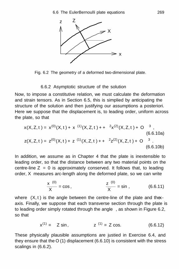
6.6 The Euler–Bernoulli plate equations 269
z Z
θ
x
X
Fig. 6.2 The geometry of a deformed two-dimensional plate.
6.6.2 Asymptotic structure of the solution
Now, to impose a constitutive relation, we must calculate the deformationand strain tensors. As in Section 6.5, this is simplified by anticipating thestructure of the solution and then justifying our assumptions a posteriori.Here we suppose that the displacement is, to leading order, uniform acrossthe plate, so that
x(X, Z, t) = x(0)(X, t) + εx(1)(X, Z, t) + +ε2x(2)(X, Z, t) + O(ε3),(6.6.10a)
z(X, Z, t) = z(0)(X, t) + εz(1)(X, Z, t) + +ε2z(2)(X, Z, t) + O(ε3).(6.6.10b)
In addition, we assume as in Chapter 4 that the plate is inextensible toleading order, so that the distance between any two material points on thecentre-line Z = 0 is approximately conserved. It follows that, to leadingorder, X measures arc-length along the deformed plate, so we can write
∂x(0)
∂X= cos θ,
∂z(0)
∂X= sin θ, (6.6.11)
where θ(X, t) is the angle between the centre-line of the plate and the x-axis. Finally, we suppose that each transverse section through the plate isto leading order simply rotated through the angle θ, as shown in Figure 6.2,so that
x(1) = −Z sin θ, z(1) = Z cos θ. (6.6.12)
These physically plausible assumptions are justified in Exercise 6.4, andthey ensure that the O (1) displacement (6.6.10) is consistent with the stressscalings in (6.6.2).

270 Asymptotic analysis
6.6.3 Leading-order equations
The deformation gradient tensor takes the form
F =(
∂xi
∂Xj
)∼(
cos θ − sin θ
sin θ cos θ
)+ε
(−ZθX cos θ x
(2)Z
−ZθX sin θ z(2)Z
)+O
(ε2), (6.6.13)
in which the leading-order term is simply a rotation through the angle θ.Hence, the strain tensor is given by
E =12(FTF − I
)∼ ε
2
(−2ZθX x
(2)Z cos θ + z
(2)Z sin θ
x(2)Z cos θ + z
(2)Z sin θ −2x
(2)Z sin θ + 2z
(2)Z cos θ
)+ O
(ε2). (6.6.14)
Since the strain is small, we can again limit our attention to the mechan-ically linear dimensional constitutive relation
S = F−1T = λTr (E)I + 2µE . (6.6.15)
We non-dimensionalise (6.6.15) using (6.6.2) and expand the stress compo-nents in powers of ε, writing
T11 = T (0)11 + εT (1)
11 + O(ε2), T31 = T (0)
31 + εT (1)31 + O
(ε2), (6.6.16)
to obtain
T (0)11 cos θ + T (0)
31 sin θ =−(1 − ν)ZθX + ν
(z
(2)Z cos θ − x
(2)Z sin θ
)(1 + ν)(1 − 2ν)
,
(6.6.17a)
0 =x
(2)Z cos θ + z
(2)Z sin θ
2(1 + ν), (6.6.17b)
T (0)31 cos θ − T (0)
11 sin θ =x
(2)Z cos θ + z
(2)Z sin θ
2(1 + ν), (6.6.17c)
0 =−νZθX + (1 − ν)
(z
(2)Z cos θ − x
(2)Z sin θ
)(1 + ν)(1 − 2ν)
,
(6.6.17d)
from which it follows that
T (0)11 = −ZθX cos θ
1 − ν2 , T (0)31 = −ZθX sin θ
1 − ν2 . (6.6.18)
6.6 The Euler–Bernoulli plate equations 271
Thus T (0)11 = T (0)
31 = 0, so the lowest-order averaged stresses are
Tx = T (1)11 , Tz = T (1)
31 , (6.6.19)
in the x- and z-directions respectively. The averaged momentum equations(6.6.8) thus give us (now dropping the superscripts)
∂2x
∂t2=
∂Tx
∂X,
∂2z
∂t2=
∂Tz
∂X− G. (6.6.20)
Next we use (6.6.10) and (6.6.16) to expand x, z and the stress componentsin the angular momentum equation (6.6.9) and simplify the result to obtain
∂M
∂X+ Tx sin θ − Tz cos θ = 0, (6.6.21)
where the bending moment is given by
M =∫ 1/2
−1/2
(T (0)
11 cos θ + T (0)31 sin θ
)Z dZ = − θX
12(1 − ν2). (6.6.22)
Equations (6.6.20) and (6.6.21) are equivalent to the dynamic beam model(4.11.8), when we identify the tangential and normal internal stresses with
T = Tx cos θ + Tz sin θ, N = Tz cos θ − Tx sin θ. (6.6.23)
However, since we have modelled the bending of a plate rather than a beam,we have obtained the constitutive relation (6.6.22) between bending mo-ment and curvature, rather than (4.11.9). One advantage of our systematicapproach is that we can determine the details of the internal stresses andstrains which are not predicted by the ad hoc theory of Section 4.9. As anillustration, we will now show briefly how the longitudinal stretching of theplate can be found.
6.6.4 Longitudinal stretching
By substituting (6.6.18) into the momentum equations (6.6.4), we find thatthe other two leading-order stress components are given by
T (0)13 =
(θX cos θ)X
2(1 − ν2)
(Z2 − 1
4
), T (0)
33 =(θX sin θ)X
2(1 − ν2)
(Z2 − 1
4
). (6.6.24)
We can also determine x(2)Z and z
(2)Z from (6.6.17) and integrate to obtain
x(2) = a(x, t) − νZ2θX sin θ
2(1 − ν), z(2) = b(x, t) +
νZ2θX cos θ
2(1 − ν), (6.6.25)

272 Asymptotic analysis
where a and b are as yet arbitrary. Note that the centre-line of the plate isdeformed to
xc(X, t) =(
x(X, 0, t)z(X, 0, t)
)∼(
x(0)(X, t) + ε2a(X, t) + · · ·z(0)(X, t) + ε2b(X, t) + · · ·
), (6.6.26)
so that∂xc
∂X∼(
cos θ
sin θ
)+ ε2
(aX
bX
)+ · · · . (6.6.27)
and arc-length s along the centre-line is thus related to X by
∂s
∂X=∣∣∣∣∂xc
∂X
∣∣∣∣ ∼ 1 + ε2 (aX cos θ + bX sin θ) + · · · . (6.6.28)
Arc-length is therefore conserved up to order ε2: this is consistent withour assumption that the plate is approximately inextensible. The small lon-gitudinal stretching that does occur is described by the O
(ε2)
correction onthe right-hand side of (6.6.28), which may be determined by analysing theconstitutive relation (6.6.15) in more detail as follows.
Considering the expressions for S11 and S33 at O(ε2), we find
T (1)11 cos θ + T (1)
31 sin θ =
(3 − 10ν + 9ν2 − ν3
)Z2θ2
X
2(1 − ν2)(1 − ν)(1 − 2ν)
+(1 − ν)
(1 + ν)(1 − 2ν)(aX cos θ + bX sin θ)
+ν
(1 + ν)(1 − 2ν)
(z
(3)Z cos θ − x
(3)Z sin θ
),
(6.6.29a)
and
0 =
(1 − 2ν + 4Z2(1 − 3ν + ν2)
)θ2X
8(1 − ν2)(1 − 2ν)
+ν
(1 + ν)(1 − 2ν)(aX cos θ + bX sin θ)
+(1 − ν)
(1 + ν)(1 − 2ν)
(z
(3)Z cos θ − x
(3)Z sin θ
), (6.6.29b)
respectively. By eliminating the final terms involving the third-order strains,we find
aX cos θ + bX sin θ =(1 − ν2) (T (1)
11 cos θ + T (1)31 sin θ
)+
(ν − 12(1 − ν)Z2
)θ2X
8(1 − ν)(6.6.30)
6.7 The linear rod equations 273
and integration with respect to Z over (−1/2, 1/2) leads to
aX cos θ + bX sin θ =(1 − ν2)T − (1 − 2ν)θ2
X
8(1 − ν). (6.6.31)
Equation (6.6.31) tells us how much the plate stretches along its centre-line. Recall that T = (Tx cos θ + Tz sin θ) is the tension in the plate, so weshould not be surprised that the stretch increases linearly with T . Perhapsless intuitive is the final term which is quadratic in the curvature and tellsus that bending the plate inevitably causes it to shrink.
6.7 The linear rod equations
6.7.1 Dimensionless equations
We now consider the deflection of a straight rod whose centre-line initiallylies along the x-axis. This time, we use as slenderness parameter
ε =√
A
L, (6.7.1)
where L is the rod length and A denotes the area of the cross-section. Aswith the linear plate equation, we suppose that the rod undergoes transversedisplacements of order W , small enough for the linear Navier equations tobe valid.
The scalings that apply to the present situation are analogous to thoseemployed in Section 6.3, namely
t =(
L
ε
√ρ
E
)t′, (6.7.2a)
(x, y, z) = L(x′, εy′, εz′), (6.7.2b)
(u, v, w) = W (εu′, v′, w′), (6.7.2c)
(τxx, τxy, τxz, τyy , τyz , τzz) =EW
L
(ετ ′
xx, τ ′xy, τ
′xz, ετ
′yy , ετ
′yz , ετ
′zz
), (6.7.2d)
so that the dimensionless Navier equations (with primes dropped) take theform
ε4 ∂2u
∂t2= ε2 ∂τxx
∂x+
∂τxy
∂y+
∂τxz
∂z, (6.7.3a)
ε2 ∂2v
∂t2=
∂τxy
∂x+
∂τyy
∂y+
∂τyz
∂z, (6.7.3b)
ε2 ∂2w
∂t2=
∂τxz
∂x+
∂τyz
∂y+
∂τzz
∂z− ε2G, (6.7.3c)
where G is defined by (6.3.8) and represents downwards gravity.

274 Asymptotic analysis
Recall that the rod is assumed to be uniform, so its cross-section occupiesa fixed two-dimensional region D in the (y, z)-plane. Our scalings for y and z
imply that D has unit area in terms of dimensional variables. In addition, wedefine the x-axis to lie along the centre-line of the rod, that is the centroidof D. These choices lead to the conditions∫∫
Ddydz = 1,
∫∫D
y dydz = 0,
∫∫D
z dydz = 0. (6.7.4)
The unit normal n to the boundary ∂D lies entirely in the (y, z)-plane,that is n = (0, ny, nz)T. If no surface tractions are applied to the rod, wetherefore have the boundary conditions
nyτxy + nzτxz = nyτyy + nzτyz = nyτyz + nzτzz = 0 on ∂D. (6.7.5)
By integrating (6.7.3) with respect to y and z, using the divergence theo-rem and applying the boundary conditions (6.7.5), we obtain the averagedequations
ε2 ∂2u
∂t2=
∂T
∂x, ε2 ∂2v
∂t2=
∂Ny
∂x, ε2 ∂2w
∂t2=
∂Nz
∂x− ε2G, (6.7.6)
where bars now denote the average over the cross-section, that is
f =∫∫
Df dydz (6.7.7)
and the tension and shear stresses are defined by
T = τxx, Ny = τxy, Nz = τxz. (6.7.8)
An equation representing net conservation of angular momentum aboutthe centre-line of the rod is found by taking y×(6.7.3c)−z×(6.7.3b) beforeintegrating over the cross-section. Again using the divergence theorem andapplying (6.7.5), we find
ε2 ∂2
∂t2(yw − zv) =
∂Mx
∂x, (6.7.9)
where
Mx = yτxz − zτxy (6.7.10)
is the torque about the centre-line. Finally, by multiplying (6.7.3a) by y
and z before integrating over the cross-section, we deduce
ε4 ∂2
∂t2(yu) = −ε2 ∂Mz
∂x− Ny, ε4 ∂2
∂t2(zu) = ε2 ∂My
∂x− Nz, (6.7.11)
6.7 The linear rod equations 275
where
My = zτxx, Mz = −yτxx (6.7.12)
are the bending moments about the y- and z-axes respectively.Now we use (6.7.11) to eliminate Ny and Nz from (6.7.6), neglecting terms
of order ε2, to obtain the equations
∂2v
∂t2= −∂2Mz
∂x2 ,∂2w
∂t2=
∂2My
∂x2 − G, (6.7.13)
governing transverse bending; these equations are equivalent to (4.5.1) and(4.5.2). Our equations of motion will be (6.7.13) combined with the axialstress balance (6.7.6a) and the axial angular momentum balance (6.7.9);with O
(ε2)
corrections neglected, these reduce to
∂T
∂x=
∂Mx
∂x= 0. (6.7.14)
6.7.2 Constitutive relations
We must now use constitutive equations to relate the axial tension T , theaxial torque Mx and the transverse bending moments My and Mz to thedeformation of the beam. After using the scalings (6.7.2), we find thatthe non-dimensionalised linear constitutive equations read
ε2τxx =ε2(1 − ν)ux + νvy + νwz
(1 + ν)(1 − 2ν), τxy =
uy + vx
2(1 + ν), (6.7.15a)
ε2τyy =ε2νux + (1 − ν)vy + νwz
(1 + ν)(1 − 2ν), τxz =
uz + wx
2(1 + ν), (6.7.15b)
ε2τzz =ε2νux + νvy + (1 − ν)wz
(1 + ν)(1 − 2ν), ε2τyz =
vz + wy
2(1 + ν). (6.7.15c)
As usual, the dependent variables are all written as asymptotic expansionsin powers of the small parameter ε2, typically
u ∼ u(0) + ε2u(1) + · · · . (6.7.16)
At leading order, we deduce from (6.7.15) that the transverse displace-ments satisfy
∂v(0)
∂y=
∂w(0)
∂z=
∂v(0)
∂z+
∂w(0)
∂y= 0 (6.7.17)
276 Asymptotic analysis
and must therefore take the form
v(0)(x, y, z, t) = a(x, t) − zc(x, t), w(0)(x, y, z, t) = b(x, t) + yc(x, t),(6.7.18)
where the arbitrary functions a and b represent uniform translations in they- and z-directions, while c corresponds to rotation of the cross-section.
By substituting for τxy and τxz from (6.7.15) into (6.7.3a) and (6.7.5), wefind that the leading-order axial displacement satisfies the two-dimensionalLaplace equation,
∂2u(0)
∂y2 +∂2u(0)
∂z2 = −∂2v(0)
∂x∂y− ∂2w(0)
∂x∂z= 0, (6.7.19a)
subject to the Neumann boundary condition
ny
(∂u(0)
∂y+
∂a
∂x− z
∂c
∂x
)+ nz
(∂u(0)
∂z+
∂b
∂x+ y
∂c
∂x
)= 0 on ∂D.
(6.7.19b)The boundary-value problem (6.7.19) may be simplified by writing u(0) inthe form
u(0)(x, y, z, t) = U(x, t) − y∂a
∂x− z
∂b
∂x+ ψ(y, z)
∂c
∂x, (6.7.20)
where U is the mean axial displacement, as yet unknown, and where ψ
satisfies
∂2ψ
∂y2 +∂2ψ
∂z2 = 0 in D, (6.7.21a)
ny
(∂ψ
∂y− z
)+ nz
(∂ψ
∂z+ y
)= 0 on ∂D. (6.7.21b)
The canonical boundary-value problem (6.7.21) is identical to that obtainedin Section 2.4 for the axial displacement in a bar undergoing pure torsion.For a given cross-sectional shape, (6.7.21) determines ψ(y, z) uniquely up tothe addition of an arbitrary constant. A simple extension of the argumentin Section 2.4 now reveals that the axial torque is related to the twist c by
Mx = R∂c
∂x, where R =
φ
(1 + ν)(6.7.22)
is the dimensionless torsional rigidity of the rod, as in Section 2.4.More importantly, since we are considering a uniform rod and Mx has
already been shown to be spatially uniform from (6.7.14), it follows that the
6.7 The linear rod equations 277
twist c must be a linear function of x, as in the exact theory of Chapter 2.Hence
∂τ(0)xy
∂x=
∂τ(0)xz
∂x= 0, (6.7.23)
so the transverse components of the Navier equation (6.7.3) reduce to
∂τ(0)yy
∂y+
∂τ(0)yz
∂z= 0,
∂τ(0)yz
∂y+
∂τ(0)zz
∂z= 0. (6.7.24)
These are just the steady plane strain equations and, subject to the zero-traction boundary conditions (6.7.5), imply that the leading-order transversestress components are all zero:
τ (0)yy = τ (0)
yz = τ (0)zz = 0. (6.7.25)
Next we determine the axial tension T = τxx. The constitutive relation(6.7.15) at order ε2 gives
τ (0)xx =
(1 − ν)u(0)x + νv
(1)y + νw
(1)z
(1 + ν)(1 − 2ν), (6.7.26a)
τ (0)yy = 0 =
νu(0)x + (1 − ν)v(1)
y + νw(1)z
(1 + ν)(1 − 2ν), (6.7.26b)
τ (0)zz = 0 =
νu(0)x + νv
(1)y + (1 − ν)w(1)
z
(1 + ν)(1 − 2ν), (6.7.26c)
from which we can eliminate v(1) and w(1) to obtain
τ (0)xx =
∂u(0)
∂x=
∂U
∂x− y
∂2a
∂x2 − z∂2b
∂x2 . (6.7.27)
By integrating over D and recalling that y and z are zero, we deduce thatthe tension is equal to the axial stretch,
T =∂U
∂x, (6.7.28)
exactly as in the uniaxial stretching discussed in Section 2.2.3.Finally, we find the bending moments My and Mz by multiplying (6.7.27)
through by y and z before integrating over D. This results in
yτ(0)xx = Mz = −Iyy
∂2a
∂x2 − Iyz∂2b
∂x2 , (6.7.29a)
zτ(0)xx = −My = −Iyz
∂2a
∂x2 − Izz∂2b
∂x2 , (6.7.29b)

278 Asymptotic analysis
where I again denotes the tensor
I =(
Iyy Iyz
Iyz Izz
)=∫∫
D
(y2 yz
yz z2
)dydz. (6.7.30)
The transverse bending equations (6.7.13) therefore reduce to
∂2a
∂t2= −Iyy
∂4a
∂x4 − Iyz∂4b
∂x4 ,∂2b
∂t2= −Iyz
∂4a
∂x4 − Izz∂4b
∂x4 − G, (6.7.31)
which, with a suitable change of notation, is the rod model (4.5.7).The ideas expounded in this section could now be combined with those
of Euler–Bernoulli plate theory to construct a systematic nonlinear rod the-ory, and thereby validate Section 4.9. Rather than performing this by-now-routine exercise, we will conclude this chapter with a brief discussion oflinear shell theory.
6.8 Linear shell theory
6.8.1 Geometry of the shell
Our final asymptotic model deals with the generalisation of Section 6.3 tocover infinitesimal deformations of a fully fledged elastic shell, as distinctfrom the weakly curved shell of Section 4.8. The initial centre-surface of theshell is parametrised by
r = rc(ξ1, ξ2), (6.8.1)
in which ξ1 and ξ2 are two spatial parameters. Since we restrict our attentionto linear elasticity, there is no need to distinguish between Lagrangian andEulerian coordinates.
We will use curvilinear coordinates (ξ1, ξ2, n) to describe any point in theplate whose position vector is
r = rc(ξ1, ξ2) + nn, (6.8.2)
where n is the unit normal to the centre-surface oriented as described below.As described in Appendix 1, the task of writing down the Navier equations isrelatively straightforward if the coordinate system (ξ1, ξ2, n) is orthogonal.This can be achieved by choosing coordinates ξ1 and ξ2 that parametriselines of curvature, with respect to which the first and second fundamentalforms of the centre-surface are both diagonal, that is
∂rc
∂ξ1· ∂rc
∂ξ2= 0,
∂2rc
∂ξ1∂ξ2· n = 0 (6.8.3)

6.8 Linear shell theory 279
(see for example Kreyszig, 1959). This choice simplifies the derivations butdoes not involve any loss of generality, since we will find that the final equa-tions may readily be expressed in any other convenient coordinate system.
We set
a1(ξ1, ξ2) =∣∣∣∣∂rc
∂ξ1
∣∣∣∣ , a2(ξ1, ξ2) =∣∣∣∣∂rc
∂ξ2
∣∣∣∣ , (6.8.4)
and hence define an orthonormal basis e1, e2, n, where
e1 =1a1
∂rc
∂ξ1, e2 =
1a2
∂rc
∂ξ2, n = e1×e2. (6.8.5)
The derivatives of these basis vectors are given by
∂e1
∂ξ1= − 1
a2
∂a1
∂ξ2e2 + κ1a1n,
∂e1
∂ξ2=
1a1
∂a2
∂ξ1e2 (6.8.6a)
∂e2
∂ξ2= − 1
a1
∂a2
∂ξ1e1 + κ2a2n,
∂e2
∂ξ1=
1a2
∂a1
∂ξ2e1, (6.8.6b)
∂n
∂ξ1= −κ1a1e1,
∂n
∂ξ2= −κ2a2e2, (6.8.6c)
where κ1 and κ2 are the principal curvatures of the centre-surface. Applyingthese identities to the parametrisation (6.8.2), we find that
∂r
∂ξ1= a1(1 − κ1n)e1,
∂r
∂ξ2= a2(1 − κ2n)e2,
∂r
∂n= n, (6.8.7)
so this coordinate system is indeed orthogonal, with scaling factors
h1 = a1(1 − κ1n), h2 = a2(1 − κ2n), h3 = 1. (6.8.8)
6.8.2 Dimensionless equations
We denote the shell thickness by h, so its surfaces (assumed stress-free) aregiven by n = ±h/2. As usual we assume here that h is constant, althoughit is straightforward to apply the same methods to a shell with non-uniformthickness. We also define L to be a typical radius of curvature, so the lengthsin the problem are non-dimensionalised via
n = hn′, (ξ1, ξ2) = L(ξ′1, ξ′2), (κ1, κ2) =
1L
(κ′1, κ
′2). (6.8.9a)
We denote the displacement field by u = u1e1+u2e2+wn. Because the shellis assumed not to be nearly flat, we must expect the in-plane and transversedisplacements to be of the same order, say
(u1, u2, w) = W (u′1, u
′2, w
′), (6.8.9b)

280 Asymptotic analysis
where W is small enough for linear elasticity to apply. The Cauchy stresstensor, relative to the curvilinear coordinate system, is now scaled using
(τ11, τ12, τ22) =EW
L
(τ ′11, τ
′12, τ
′22), (τ13, τ23, τ33) =
ε2EW
L
(τ ′13, τ
′23, τ
′33),
(6.8.9c)
as distinct from (6.3.4), and the appropriate time-scale is now
t = L
√ρ
Et′. (6.8.9d)
Gravity is assumed to act in the direction −k and is represented by itsdimensionless components along each of the basis vectors, defined as
g1 = −ρgL2
EW(k · e1) , g2 = −ρgL2
EW(k · e2) , g3 = −ρgL2
EW(k · n) .
(6.8.10)
To avoid clutter, we henceforth drop the primes on the dimensionless vari-ables.
6.8.3 Leading-order equations
The Navier equations and linear constitutive relations in an arbitrary orthog-onal coordinate system may be found in the Appendix. As in the previoussections, we simplify the dimensionless equations by letting ε → 0 to obtain
∂2u1
∂t2− g1 =
1a1a2
∂
∂ξ1(a2τ11) +
∂
∂ξ2(a1τ12) + τ12
∂a1
∂ξ2− τ22
∂a2
∂ξ1
,
(6.8.11a)
∂2u2
∂t2− g2 =
1a1a2
∂
∂ξ1(a2τ12) +
∂
∂ξ2(a1τ22) + τ12
∂a2
∂ξ1− τ11
∂a1
∂ξ2
,
(6.8.11b)
∂2w
∂t2− g3 = κ1τ11 + κ2τ22, (6.8.11c)
at leading order. Once we have used the constitutive relations to expressτ11, τ12 and τ22 in terms of the displacements, (6.8.11) will give us threeequations for u1, u2 and w.
The constitutive relations imply that the displacement components areall independent of n to leading order. Furthermore, the dimensionless con-stitutive relation for τ33 reads
νe11 + νe22 + (1 − ν)e33
(1 + ν)(1 − 2ν)= ε2τ33, (6.8.12)

6.8 Linear shell theory 281
which we can use to express e33 in terms of e11 and e22, and hence obtain
τ11 =e11 + νe22
1 − ν2 , τ22 =νe11 + e22
1 − ν2 . (6.8.13)
The relevant leading-order strain components are
e11 =1a1
(∂u1
∂ξ1+
u2
a2
∂a1
∂ξ2
)− κ1w, (6.8.14a)
e22 =1a2
(∂u2
∂ξ2+
u1
a1
∂a2
∂ξ1
)− κ2w, (6.8.14b)
e33 =1ε
∂w
∂n, (6.8.14c)
while the leading-order in-plane shear stress reads
τ12 =1
2(1 + ν)a1a2
a1
∂u1
∂ξ2− u1
∂a1
∂ξ2+ a2
∂u2
∂ξ1− u2
∂a2
∂ξ1
. (6.8.15)
Space does not permit a detailed discussion of the system (6.8.11)–(6.8.15)for u1, u2 and w, although some indication of the richness of its solutionsmay be discerned in Exercises 6.6 and 6.7. Here we will merely add a fewgeneral observations.
Although we have derived our leading-order model using the specific co-ordinate system defined by (6.8.2), it may be cast in an invariant form thatis independent of the parametrisation chosen. The momentum equations(6.8.11) may be written as
∂2u
∂t2− g = ∇ · τ ,
∂2w
∂t2− g3 = K : τ , (6.8.16)
where u = u − wn is the in-plane displacement, ∇ is the surface gradientoperator, τ is in-plane stress and K is the curvature tensor. In the samenotation, the in-plane stress satisfies the constitutive relation
τ =1
1 + νE +
ν
1 − ν2 Tr(E)I, (6.8.17)
where the surface strain tensor is given by
E =12
∇u + (∇u)T
− wK. (6.8.18)
The theory just derived describes deformations in which the in-plane ten-sions dominate and the bending stiffness is negligible. However, our modelallows for nontrivial displacements that cause zero leading-order stress. Forexample, if we let the shell tend to a flat sheet so that κ1 = κ2 = 0, then thenormal displacement w decouples entirely from the in-plane stresses and isarbitrary in the absence of bending stiffness. Similarly, a cylinder bent about

282 Asymptotic analysis
its generators offers no resistance to a large class of displacements, as shownin Exercise 6.6. More generally, elimination of w from (6.8.14) and (6.8.15)shows that zero stress results from in-plane displacement fields satisfyingthe system of partial differential equations(
a2κ2 00 a2
)∂
∂ξ1
(u1
u2
)+(
0 −a1κ1
a1 0
)∂
∂ξ2
(u1
u2
)=(
κ1u1∂a2/∂ξ1 − κ2u2∂a1/∂ξ2
u1∂a1/∂ξ2 + u2∂a2/∂ξ1
). (6.8.19)
It is easy to calculate that the characteristic curves for this system are givenby
dξ2
dξ1= ±a1
a2
√−κ1
κ2. (6.8.20)
Hence (6.8.19) is elliptic, parabolic or hyperbolic, depending on the sign ofthe Gaussian curvature, exactly as in Section 4.8, and we can expect theexistence of a zero-stress mode compatible with given boundary conditionsto depend strongly on this type.
In cases where the imposed boundary conditions are compatible with(6.8.19), the displacement field is not uniquely determined by our model.The resolution of the indeterminacy would require us to consider a geomet-rically nonlinear limit similar to that which led to the von Karman theory inSection 6.5. This would describe weakly nonlinear deformations of a shell, inwhich the in-plane stresses and bending stiffness balance, but this is beyondthe scope of this book.
6.9 Concluding remarks
It is comforting to see that some of the approximate models in Chapter 4,which were derived on the basis of intuition and plausibility, can be recoveredby systematic perturbation procedures. The asymptotic approach outlinedhere, however, provides us with a much more detailed picture of the stressfield than the approximate theories alone. For instance, we have been ableto resolve its three-dimensional structure in the vicinity of the boundariesand elucidate the Saint-Venant principle. Additionally, we have seen thefascinating challenges posed by geometric nonlinearity. Perhaps the biggestsurprise is that the familiar membrane terms in equations like (4.4.8) actuallyarise, and can only be derived, from geometrically nonlinear elasticity.
A recurrent pattern in the asymptotic methodology has emerged: first,the geometry of the solid suggests particular scalings for the displacement

Exercises 283
field; then, the stress components are rescaled so as to balance as manyterms as possible in the Navier equations; finally, these equations are anal-ysed asymptotically, or, if we are lucky, by suitable global averaging overboundary layers.
We have only been concerned with plates, shells and rods with uniformthickness or cross-section and comparable elastic moduli. If the thickness ofthe plate were to vary rapidly with a typical length-scale L, a quitenew theory would be needed. The same would be true if µ/λ 1 (i.e. ν
is close to 1/2). In such cases, we would have to state precisely what arethe relative orders of magnitude of the various small parameters involved,namely ε, /L, and µ/λ. In particular, there is no reason to expect that thelimits ε → 0 and µ/λ → 0 would commute.
Exercises
6.1 Reconsider the antiplane strain example of Section 6.2, this timeassuming that the bottom and top of the sheet are subjected totractions τyz = σ−(x) and τyz = σ+(x) on y = 0 and y = h, respec-tively.
(a) Non-dimensionalise using the same perturbation scheme as inSection 6.2 away from the edges. Rescaling the surface trac-tions as σ±(x) = (µW/h)σ′
±(x), derive the solvability condi-tion σ′
+ − σ′− = O
(ε2).
(b) Hence, letting σ+ = σ− + ε2σ, deduce from the solvabilitycondition at O
(ε2)
that
d2w0
dx2 + σ = 0.
6.2 Repeat the linear rod derivation from Section 6.7 using the fast time-scale
t =(
εL
√ρ
E
)t′.
Show that the decompositions (6.7.18), (6.7.20) still apply, where thefunctions a, b, c and U satisfy the equations
∂2a
∂t2= 0,
∂2b
∂t2= 0, (Iyy + Izz)
∂2c
∂t2= R
∂2c
∂x2 ,∂2U
∂t2=
∂2U
∂x2 .
[This shows that longitudinal and torsional waves occur over a muchshorter time-scale than the flexural waves considered in Section 6.7.]

284 Asymptotic analysis
6.3 Derive the governing equations for a weakly curved shell as follows.Suppose the upper and lower surfaces of the shell are given in di-mensionless variables by
Z = H(X, Y ) ± 12,
so that H(X, Y ) represents the undeformed centre-surface, and thestress-free boundary conditions read
T13 =∂H
∂XT11 +
∂H
∂YT12, T23 =
∂H
∂XT21 +
∂H
∂YT22,
T33 =∂H
∂XT31 +
∂H
∂YT32,
on Z = H ± 1/2.Use the asymptotic approach of Section 6.5 to derive the equations
−∇4A =∂2w
∂X2∂2w
∂Y 2 −(
∂2w
∂X∂Y
)2
+∂2H
∂Y 2∂2w
∂X2 − 2∂2H
∂X∂Y
∂2w
∂X∂Y+
∂2H
∂X2∂2w
∂Y 2
and
∂2w
∂t2+ G +
∇4w
12(1 − ν2)=
∂2(H + w)∂Y 2
∂2A
∂X2
− 2∂2(H + w)
∂X∂Y
∂2A
∂X∂Y+
∂2(H + w)∂X2
∂2A
∂Y 2 .
Show that these reduce to (4.8.9) and (4.8.11) when |w| |H|.6.4 Show that the strain tensor in Section 6.6 is given by
E =12
(x2
X + z2X − 1 ε−1 (xXxZ + zXzZ )
ε−1 (xXxZ + zXzZ ) ε−2(x2
Z + z2Z
)− 1
).
Hence, show that T is O(ε−2E
)unless (6.6.10) is assumed. Further,
show that the components of S must be at most O (εE) for thescaling (6.6.2) to hold and therefore that(
∂x(0)
∂X
)2
+
(∂z(0)
∂X
)2
= 1,
(∂x(1)
∂Z
)2
+
(∂z(1)
∂Z
)2
= 1,
∂x(0)
∂X
∂x(1)
∂Z+
∂z(0)
∂X
∂z(1)
∂Z= 0.
From this, justify (6.6.11) and (6.6.12).
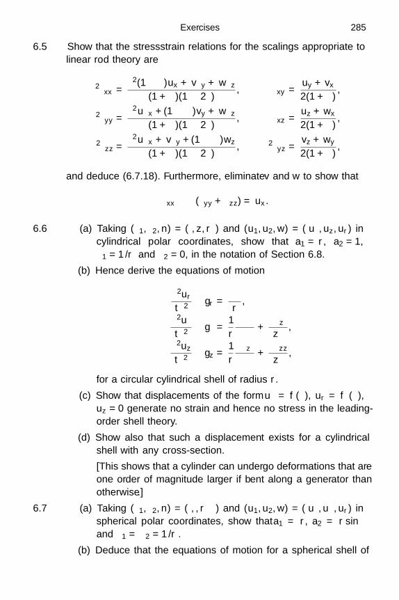
Exercises 285
6.5 Show that the stress–strain relations for the scalings appropriate tolinear rod theory are
ε2τxx =ε2(1 − ν)ux + νvy + νwz
(1 + ν)(1 − 2ν), τxy =
uy + vx
2(1 + ν),
ε2τyy =ε2νux + (1 − ν)vy + νwz
(1 + ν)(1 − 2ν), τxz =
uz + wx
2(1 + ν),
ε2τzz =ε2νux + νvy + (1 − ν)wz
(1 + ν)(1 − 2ν), ε2τyz =
vz + wy
2(1 + ν),
and deduce (6.7.18). Furthermore, eliminate v and w to show that
τxx − ν (τyy + τzz) = ux.
6.6 (a) Taking (ξ1, ξ2, n) = (θ, z, r) and (u1, u2, w) = (uθ, uz, ur) incylindrical polar coordinates, show that a1 = r, a2 = 1,κ1 = 1/r and κ2 = 0, in the notation of Section 6.8.
(b) Hence derive the equations of motion
∂2ur
∂t2− gr =
τθθ
r,
∂2uθ
∂t2− gθ =
1r
∂τθθ
∂θ+
∂τθz
∂z,
∂2uz
∂t2− gz =
1r
∂τθz
∂θ+
∂τzz
∂z,
for a circular cylindrical shell of radius r.
(c) Show that displacements of the form uθ = f(θ), ur = f ′(θ),uz = 0 generate no strain and hence no stress in the leading-order shell theory.
(d) Show also that such a displacement exists for a cylindricalshell with any cross-section.
[This shows that a cylinder can undergo deformations that areone order of magnitude larger if bent along a generator thanotherwise.]
6.7 (a) Taking (ξ1, ξ2, n) = (θ, φ, r) and (u1, u2, w) = (uθ, uφ, ur) inspherical polar coordinates, show that a1 = r, a2 = r sin θ
and κ1 = κ2 = 1/r.
(b) Deduce that the equations of motion for a spherical shell of

286 Asymptotic analysis
radius r are
∂2ur
∂t2− gr =
τθθ + τφφ
r,
∂2uθ
∂t2− gθ =
1r sin θ
[∂
∂θ(sin θτθθ) +
∂τθφ
∂φ− τφφ cos θ
],
∂2uφ
∂t2− gφ =
1r sin θ
[∂
∂θ(sin θτθφ) +
∂τφφ
∂φ+ τθφ cos θ
].
(c) Suppose that the strain is identically identically zero. Elim-inate ur and uθ (or use (6.8.19) directly) to show that uφ
satisfies the equation
∂2uφ
∂φ2 + sin2 θ∂
∂θ
(sin θ
∂
∂θ
( uφ
sin θ
))= 0,
while∂uθ
∂φ= − sin2 θ
∂
∂θ
( uφ
sin θ
), and ur =
∂uθ
∂θ.
By seeking separable solutions that are periodic in φ, showthat possible solutions for uφ are
(i) uφ = sin θ,
(ii) uφ = sin θ log(tan(θ/2)
),
(iii) uφ = sin(kφ) sin θ tank(θ/2),
and find the corresponding expressions for uθ and ur .[Hint: show that sin θ ∂/∂θ = ∂/∂ξ with ξ = log tan(θ/2).]
(d) Note that (i) is simply a rigid body motion. Show that theremaining solutions are physically unacceptable if the shellis a complete sphere. Discuss solutions (ii) and (iii) for hemi-spherical shells. Show that (ii) gives rise to a multi-valued dis-placement. To which physical situation could it correspond?

7
Fracture and contact
7.1 Introduction
Fracture describes the behaviour of thin cracks, like the one illustrated inFigure 7.1, in an otherwise elastic material. The crack itself is a thin void,whose faces are usually assumed to be stress-free. When a solid containinga crack is stressed, we will find that the stress is localised near the cracktip, becoming singular if the tip is sharp. We will see that the strengthof the singularity can be characterised by a stress intensity factor, whichdepends on the size of the crack and on the applied stress. This factor deter-mines the likelihood that a crack will grow and, therefore, that the solid willfail.†
On the other hand, contact refers to the class of problems in which twoelastic solid bodies are brought into contact with each other, as illustrated inFigure 7.2. When the material properties are the same in the two bodies, thegeometrical configuration near the edge of the contact region is apparentlysimilar to that of fracture, with voids now outside the contact set, that is, theset of points at which the two solids are in contact. The mathematical setupof such problems does therefore have some similarity with fracture, but, inthe steady state, there is one crucial difference. Whereas much of the studyof fracture concerns cracks of prescribed length, in contact problems thecontact set itself is often unknown in advance. They are thus known as freeboundary problems, that is problems whose geometry must be determinedalong with the solution. An example of such a problem is to determine howthe contact area between a car tyre and the road depends on the inflationpressure.
†The reader may be reassured to know that, although several cracks emanate from many rivetsin an airliner, they are carefully monitored to ensure that none of them is dangerous.
287

288 Fracture and contact
crack tip
crack faces
Fig. 7.1 Definition sketch of a thin crack.
contact set
Fig. 7.2 Definition sketch for contact between two solids.
7.2 Static brittle fracture
7.2.1 Physical background
In Section 2.2.5, we proposed the idea that the theory of linear elasticitymay fail when some stress components in a solid reach a critical value atsome point. While this statement is generally true, the way in which failureoccurs can be very different for different solids, or even for the same solidunder different loading conditions. This section will focus on the simplestmathematical model for one type of failure, namely brittle fracture.
The adjective “fractured” is usually used to describe configurations wherea continuum solid has developed cracks, which are very thin stress-free voids.These voids are characterised by being thin in only one direction so that theyare nearly slits in a two-dimensional solid (see Figure 7.1). Thus a crack hastwo faces with a common perimeter which is called the crack tip, and thetip is just two points in the two-dimensional case. Cracks are often initiated
7.2 Static brittle fracture 289
at the surface of the material, which is usually the only place where theycan be discerned by the naked eye.
Brittle fracture covers that class of fractures, such as windscreen shatter-ing, where the initiation and growth of the crack do not affect the materialmodelling, which is still governed by the Navier equations. Such a situationmight not be true for a metal, where quite a large region near the cracktip may have to be modelled using plasticity rather than elasticity equa-tions; then the fracture is called ductile, and we will discuss this further inChapter 8.
We can say little more here about the physical background of this vastand important subject. However, we urge the reader to think intuitively thatfracturing, i.e. crack growth, is basically a local stress-relieving mechanism.As a crack grows, the strain energy in the evolving fractured configurationis less than the value it would have taken had the crack not evolved. Thisargument suggests that the criterion for a crack to evolve under a smallincrease of loading is that the release, −δW, of strain energy resulting froma small growth δA in the crack face area is such that
∫∫∫V−δW dx > δS, (7.2.1)
where V denotes the region excluding the crack and δS is the surface energyof the area δA. In principle, δS could be estimated from molecular consid-erations but, in the theory of Griffith cracks (see, for example, Sneddon &Lowengrub, 1969, Chapter 1; Freund, 1989, Chapter 1) δS is thought of asresulting from an effective surface tension γ; in this case, δS = γδA.
It is interesting to compare fracture with the more familiar failure of aliquid, which cavitates when the pressure is too low, so that the molecularbonds weaken and allow the molecules to form a vapour. This often results inthe appearance of a spherical bubble, whereas a crack morphology is usuallythe one preferred by solids. The difference in behaviour arises because it iseasier to create new interface between a liquid and a vapour than it is tocreate new interface between a solid and a void. Hence a crack can growmost easily by creating new surface energy just in the vicinity of the cracktip. It is also instructive to contrast fracture, which often occurs as a resultof some remote loading process, with the drilling of a thin hole through thesolid (for example using a shaped charge; see Section 3.6). It is an everydayobservation that the energy required to drill a hole per unit surface areagenerated is greater than that required to cleave the material using an axe.

290 Fracture and contact
c−c
τyz = 0
(a)τyz → σIII
τyz → σIII
x
(b)
y
x
σIII
y
σIII
Fig. 7.3 (a) A Mode III crack. (b) A cross-section in the (x, y)-plane.
7.2.2 Mode III cracks
Let us now investigate the predictions of the Navier model for linear elas-ticity in the presence of a crack. The very simplest configuration is that ofa crack in antiplane strain, which is called a Mode III crack, as illustratedin Figure 7.3. Although this configuration is not so important in practice,it is much simpler mathematically than Mode I and II cracks, which will beintroduced later.
We will consider a planar crack whose faces lie close to the (x, z)-planebetween the crack tips x = ±c, y = 0. The physical set-up is that of alarge cracked slab being sheared at infinity in the (y, z)-plane with a shearstress σIII. Assuming that the faces of the crack are stress free, we find thatthe mathematical model for the displacement w(x, y) in the z-direction is
∇2w = 0 (7.2.2a)
everywhere except on y = 0, |x| < c, with
µ∂w
∂y→ σIII as x2 + y2 → ∞, (7.2.2b)
µ∂w
∂y= 0 on y = 0, |x| < c. (7.2.2c)
There is a fundamental difference between (7.2.2) and most of the bound-ary value problems we have thus far considered for elastostatics, namelythat the boundary on which the Neumann data (7.2.2c) are prescribed isnot smooth at the crack tip. To see the kind of difficulty that this can cause,suppose we were to shift the origin to (−c, 0) and concentrate on the regionnear the crack tip. Then we would need to find a displacement field in which∇2w = 0 everywhere except on y = 0, x > 0, with
µ∂w
∂y= 0 on y = 0, x > 0. (7.2.3)
7.2 Static brittle fracture 291
By separating the variables in polar coordinates (r, θ), we immediately seethat w can be any function of the form
w = Arn/2 cos(nθ/2) = A Re(zn/2
), (7.2.4)
where z = reiθ , A is a constant and n is an integer. The corresponding stresscomponents are given by
τrz =µnA
2rn/2−1 cos(nθ/2), τθz = −µnA
2rn/2−1 sin(nθ/2). (7.2.5)
This plethora of solutions gives us the strong hint that we will not be ableto solve (7.2.2) uniquely unless we supply some extra information about thebehaviour of w near (±c, 0). We also note that, whenever n is not an evenpositive integer, the stress is non-analytic at the crack tip r = 0, and, ifn < 2, the stress is not even bounded.
From a mathematical point of view it is natural to ask whether the solutionof (7.2.2) must be singular at (±c, 0) and, if so, what is the mildest singularitywhich we have to endure. To answer these questions, one possibility is toround off the crack, that is, to replace it with a thin but smooth boundary.A particularly convenient shape is the ellipse
x2
c2 cosh2 ε+
y2
c2 sinh2 ε= 1, (7.2.6)
which is smooth for all positive ε but approaches the slit geometry of Fig-ure 7.3(b) in the limit ε → 0. Now we can easily solve Laplace’s equation byintroducing elliptic coordinates defined by
z = x + iy = c cosh ζ, where ζ = ξ + iη, (7.2.7a)
so that
x = c cosh ξ cos η, y = c sinh ξ sin η. (7.2.7b)
Since the map (7.2.7) from z to ζ is conformal except on y = 0, |x| < c,Laplace’s equation is preserved and the model (7.2.2) becomes
∂2w
∂ξ2 +∂2w
∂η2 = 0 in ξ > ε (7.2.8a)
with∂w
∂ξ= 0 on ξ = ε, (7.2.8b)

292 Fracture and contact
z
Im z
Re z
r1rr2
θ2 θ
c
θ1
−c
Fig. 7.4 Definition sketch for the function√
z2 − c2 .
and, since y ∼ (c/2)eξ sin η as ξ → ∞,
w ∼ cσIII
2µeξ sin η as ξ → ∞. (7.2.8c)
By separating the variables, we easily find the solution
w =cσIII
2µsin η
(eξ + e2ε−ξ
). (7.2.9)
We thus have a unique displacement field for any positive value of ε and,when we let ε → 0, we obtain the solution of the crack problem as
w =cσIII
µIm (sinh ζ) . (7.2.10)
Using (7.2.7), this can be written as
w =σIII
µIm
(√z2 − c2
), (7.2.11)
where the square root is defined to be√z2 − c2 ≡ √
r1r2 ei(θ1 +θ2 )/2, (7.2.12)
with r1, r2, θ1 and θ2 defined as shown in Figure 7.4. The angles are takento lie in the ranges −π < θj < π, so that a branch cut lies along the crackbetween z = −c and z = c (see, for example, Priestley, 2003, Chapter 9). Asshown in Figure 7.5, the displacement w is discontinuous across this branchcut.

7.2 Static brittle fracture 293
Fig. 7.5 Displacement field for a Mode III crack.
Despite its simplicity, the formula (7.2.11) lies at the very heart of the the-ory of brittle fracture. It reveals the famous square root singularity in whichthe elastic displacement varies as the square root of the distance from thecrack tip.† By rounding off the crack before taking the limit ε → 0, we havemanaged to select one of the many possible singular solutions suggested by(7.2.4). This dependence immediately implies that the stress tensor, whosenon-zero components are
τxz = µ∂w
∂xand τyz = µ
∂w
∂y, (7.2.13)
diverges as the inverse square root of the distance from the tip. This physi-cally unacceptable consequence renders the Navier model invalid sufficientlyclose to the tip, but there are several ways of recovering from this setback,including the following.
(i) Rounding the tipThis is the approach adopted above when considering the elliptical crack(7.2.6), and it is easily shown, using this example, that the stress at thecrack tip is given approximately by
τyz ∼ 2σIII
√c
r0(7.2.14)
when r0, the tip radius of curvature, is small (Exercise 7.1).(ii) Plastic zone
Even if the tip is rounded, (7.2.14) shows that the stress may still become
†A similarly fundamental square root singularity arises in the mathematically analogous theoryof aerofoils; (see, for example, Batchelor, 2000, p. 467).
x
y
w
294 Fracture and contact
large enough for the material to yield plastically if r0 is sufficiently small.This suggests the introduction of a plastic zone near the tip, and this alsohas the effect of preventing the stress from growing without bound. Wewill discuss plasticity further in Chapter 8.
(iii) Tip cohesionIn (7.2.2), we assumed that the two faces of the crack exert no traction oneach other. Instead we might suppose that there is an effective cohesionbetween the faces, so that (7.2.2c) is replaced by
µ∂w
∂y= f(x) on y = 0, |x| < c, (7.2.15)
where f(x) models the cohesive effect of intermolecular bonding, whichwill be strongest near the crack tip. As shown in Exercise 7.3, a suitablechoice of f can be made to ensure that the stress remains finite every-where.
Rather than pursue any of these possibilities for “regularising” our modelnear the crack tip, we will show how the existence of the square root in(7.2.11) can be exploited to great practical effect. The result (7.2.11) pre-dicts that any critical stress, no matter how large, will always be attainedsufficiently close to the crack tip. Hence, let us return to the discussionof (7.2.1) and consider whether or not the crack is dangerous, that is,whether or not it will propagate. This poses the question: “is the localstress large enough for it to do sufficient work to create new surface en-ergy at the crack tip when σIII is increased slightly?” The following answerto this question has formed the basis of the theory of fracture for manydecades.
We note that, in the material ahead of the crack tip (c, 0), the only non-zero stress component at the crack plane y = 0 is τyz and that
limx↓c
τyz(x, 0)√
x − c = σIII√
c/2. (7.2.16)
Hence, no matter which of the mechanisms such as (i)–(iii) above preventsthe stress from becoming infinite in practice, it will have to be triggeredby a local stress intensification that is proportional to the inverse squareroot of distance from the tip. It turns out that the selection of the valuen = 1 in (7.2.4) is generic for all Mode III cracks. Every such crack tip ischaracterised by the limit defined in (7.2.16) and, conventionally, this limitis written as
limx↓c
τyz(x, 0)√
x − c =KIII√
2π. (7.2.17)

7.2 Static brittle fracture 295
The stress intensity factor KIII is the parameter that characterises thepropensity of the crack to propagate. For the crack modelled by (7.2.2),for example, we find that KIII =
√πcσIII. We postulate that the crack will
propagate if KIII exceeds a critical value, which must be determined ei-ther from (i)–(iii) above or from experiment, and which we expect to beproportional to the surface energy γ. Under this postulate, (7.2.16) im-mediately reveals that a Mode III crack is more likely to grow if it islonger or subject to greater stress. We emphasise that a consequence ofthis postulate is that KIII is the only piece of information concerning theglobal stress field that is relevant for deciding whether or not the crackpropagates.
We will shortly find that the concept of a stress intensity factor appliesto many other crack configurations, but first let us review the mathematicalchallenges posed by problems like (7.2.2).
7.2.3 Mathematical methodologies for crack problems
Now let us quickly review some different approaches that we might haveadopted to obtain (7.2.11) had we not been able to utilise elliptic coordinatesand take the limit as ε → 0. Four possibilities are the following.
(i) We could conformally map the region outside the cut y = 0, |x| < c ontothe exterior of a circle and solve Laplace’s equation in polar coordinates.This is effectively what we have done to obtain (7.2.11), but in principlethe method applies to any antiplane strain crack problem where the rel-evant conformal map can be found by inspection. However, it cruciallyrelies on the fact that Laplace’s equation is invariant under conformalmapping; as we will see below, considerably more effort is required togeneralise this approach to the biharmonic equation.
(ii) We could represent w(x, y) as a suitable distribution of functions that aresingular on the slit. This approach allows most scope for physical intuition.Noting that tan−1(y/x) is a solution of Laplace’s equation except at theorigin and on a branch cut from the origin, we can directly computethat
µw = σIIIy − σIII
π
∫ c
−c
ξ tan−1((x − ξ)/y
)√c2 − ξ2
dξ (7.2.18)
is equivalent to (7.2.11), as shown in Exercise 7.2. Thus w can be thoughtof as resulting from the imposed stress together with a distribution ofwhat are called virtual dislocations, and we will return to this idea in
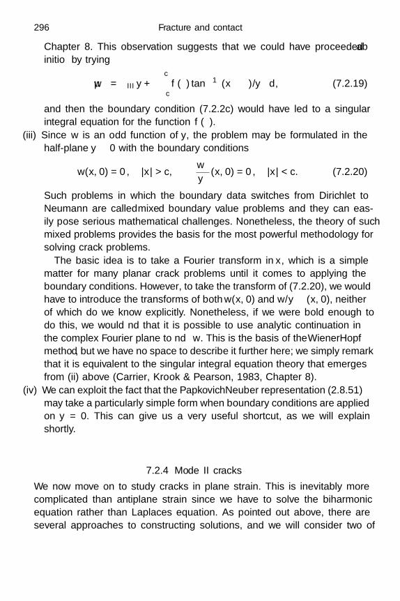
296 Fracture and contact
Chapter 8. This observation suggests that we could have proceeded abinitio by trying
µw = σIIIy +∫ c
−cf(ξ) tan−1((x − ξ)/y
)dξ, (7.2.19)
and then the boundary condition (7.2.2c) would have led to a singularintegral equation for the function f(ξ).
(iii) Since w is an odd function of y, the problem may be formulated in thehalf-plane y 0 with the boundary conditions
w(x, 0) = 0, |x| > c,∂w
∂y(x, 0) = 0, |x| < c. (7.2.20)
Such problems in which the boundary data switches from Dirichlet toNeumann are called mixed boundary value problems and they can eas-ily pose serious mathematical challenges. Nonetheless, the theory of suchmixed problems provides the basis for the most powerful methodology forsolving crack problems.
The basic idea is to take a Fourier transform in x, which is a simplematter for many planar crack problems until it comes to applying theboundary conditions. However, to take the transform of (7.2.20), we wouldhave to introduce the transforms of both w(x, 0) and ∂w/∂y(x, 0), neitherof which do we know explicitly. Nonetheless, if we were bold enough todo this, we would find that it is possible to use analytic continuation inthe complex Fourier plane to find w. This is the basis of the Wiener–Hopfmethod, but we have no space to describe it further here; we simply remarkthat it is equivalent to the singular integral equation theory that emergesfrom (ii) above (Carrier, Krook & Pearson, 1983, Chapter 8).
(iv) We can exploit the fact that the Papkovich–Neuber representation (2.8.51)may take a particularly simple form when boundary conditions are appliedon y = 0. This can give us a very useful shortcut, as we will explainshortly.
7.2.4 Mode II cracks
We now move on to study cracks in plane strain. This is inevitably morecomplicated than antiplane strain since we have to solve the biharmonicequation rather than Laplace’s equation. As pointed out above, there areseveral approaches to constructing solutions, and we will consider two of

7.2 Static brittle fracture 297
xx
y yσII
σIIσII
σII Ω
(a) (b)
∂Ω
Fig. 7.6 (a) A planar Mode II crack. (b) The regularised problem of a thin ellipticalcrack.
them in detail. We will start by using a conformal mapping technique, whichis analogous to that employed in Section 7.2.2 for Laplace’s equation. Asbefore, we will regularise the problem by considering an elliptical crack,with a small but finite diameter of order ε, and then letting ε → 0. Then,we will see how Papkovich–Neuber potentials provide an alternative shortcutto the solution.
In a planar Mode II crack, a far-field shear stress σII (not to be confusedwith σ11) parallel to the plane of the crack is applied, as shown in Figure 7.6.We denote the two-dimensional region outside the crack by Ω and the ellipti-cal boundary of the crack by ∂Ω. This is evidently a plane strain problem, sowe employ an Airy stress function which, as usual, satisfies the biharmonicequation in Ω. If the crack is stress-free then, as shown in Section 2.6.3, wecan without loss of generality impose the boundary conditions
∇A = 0 on ∂Ω. (7.2.21)
The imposed uniform shear stress far from the crack implies that A has theasymptotic behaviour
A ∼ −σIIxy as x2 + y2 → ∞. (7.2.22)
We recall from Section 2.6 that the general solution of the two-dimensionalbiharmonic equation may be written in the form
A = Rezf(z) + g(z)
, (7.2.23)
where f and g are any two analytic functions of z = x + iy. To transformthe boundary conditions for A into conditions on f and g, it is helpful towrite (7.2.23) in the form
A =12zf(z) + g(z) + zf(z) + g(z)
, (7.2.24)
298 Fracture and contact
where f is the conjugate function to f , that is f(z) ≡ f(z). From (7.2.21),we deduce that
∂A
∂z=
12
(∂A
∂x− i
∂A
∂y
)= 0 (7.2.25)
on ∂Ω and, hence, by using (7.2.24), we obtain the condition
zf ′(z) + f(z) + g′(z) = 0 on ∂Ω. (7.2.26)
In addition, the far-field behaviour (7.2.22) implies that f and g satisfy
f(z) → 0, g(z) ∼ iσII
2z2 as z → ∞. (7.2.27)
Amazingly, the two functions f and g can be determined using only thefact that they are both analytic in Ω and the conditions (7.2.26) and (7.2.27).However, it is not immediately obvious how to do this, and the task isgreatly simplified by conformally mapping Ω onto a region that is easier tomanipulate. Here we note that the region outside our elliptical crack is theimage of the unit disc under the conformal mapping
z = ω(ζ) = aζ +b
ζ, (7.2.28)
where a and b are real constants with b > a > 0. The principal radii of theellipse are (a + b) and (a − b), so that
a =ceε
2, b =
ce−ε
2, (7.2.29)
in the terminology of Section 7.2.2. We also introduce the notation
F (ζ) = f(ω(ζ)
), G(ζ) = g
(ω(ζ)
)(7.2.30)
for the transformed versions of f and g. Thus F is analytic in the unit disc|ζ| 1, and G is analytic apart from a double pole at the origin, where
G(ζ) ∼ iσIIb2
2ζ2 as ζ → 0. (7.2.31)
The boundary condition (7.2.26) is transformed to
−F (1/ζ) =ω(1/ζ)F ′(ζ)
ω′(ζ)+
G′(ζ)ω′(ζ)
at |ζ| = 1, (7.2.32)
where
ω(1/ζ) =a + bζ2
ζ, ω′(ζ) =
aζ2 − b
ζ2 , (7.2.33)

7.2 Static brittle fracture 299
and we use the fact that ζ = 1/ζ on the unit circle. Provided b > a > 0, themap z = ω(ζ) is conformal and hence ω′(ζ) is nonzero in the unit disc. Theonly singularity in the right-hand side of (7.2.32) therefore arises from thepole in G(ζ) at the origin, where we find that
G′(ζ)ω′(ζ)
∼ iσIIb
ζas ζ → 0. (7.2.34)
Let us subtract this from both sides of (7.2.32) to remove the singularityfrom the right-hand side and thus obtain
−F (1/ζ) − iσIIb
ζ=
ζ2G′(ζ) + ζ(a + bζ2
)F ′(ζ)
aζ2 − b− iσIIb
ζat |ζ| = 1.
(7.2.35)Now we arrive at the crux of the argument. The left-hand side of (7.2.35)
is analytic in |ζ| 1, while the right-hand side is analytic in |ζ| 1. We cantherefore use (7.2.35) to analytically continue the left-hand side into |ζ| < 1and hence obtain a function that is analytic on the entire complex planeand, because of (7.2.27), tends to zero as ζ → ∞ (see, for example, Carrier,Krook & Pearson, 1983, Section 2.8). According to Liouville’s theorem, theonly function that has these properties is the zero function, and we deducethat the left- and the right-hand sides of (7.2.35) must both be identicallyzero. We can therefore evaluate the function F (ζ) as
F (ζ) = iσIIbζ (7.2.36)
and, by using this expression in the right-hand side of (7.2.35), we obtain
G′(ζ) = −iσIIb2(
ζ +1ζ3
). (7.2.37)
By integrating with respect to ζ and ignoring an irrelevant constant of in-tegration, we thus obtain
G(ζ) =iσIIb
2
2
(1ζ2 − ζ2
). (7.2.38)
Finally, by using the inverse mapping
ζ =z −
√z2 − 4ab
2a, (7.2.39)

300 Fracture and contact
where the square root is again defined by (7.2.12), we evaluate the functionsf and g in terms of the original variable z as
f(z) =iσIIb
2a
(z −
√z2 − 4ab
), (7.2.40a)
g(z) =iσII
4a2
(a2 − b2)(z2 − 2ab) + (a2 + b2)z
√z − 4ab
. (7.2.40b)
When substituting these into the formula (7.2.23) for A, we simplify theresulting expression by letting the crack thickness tend to zero, so that a
and b both tend to c/2, and thus obtain
A =σII
2Im
(z − z)
√z2 − c2
. (7.2.41)
By using the chain rules
∂
∂x=
∂
∂z+
∂
∂z,
∂
∂y= i
(∂
∂z− ∂
∂z
), (7.2.42)
as shown in Exercise 7.4, we can recover the stress components as
τxx = Re−zf ′′(z) − g′′(z) + 2f ′(z)
=
σII
2Im
4z3 + c2 (z − 5z)
(z2 − c2)3/2
, (7.2.43a)
τxy = Imzf ′′(z) + g′′(z)
=
σII
2Re
2z3 + c2 (z − 3z)
(z2 − c2)3/2
, (7.2.43b)
τyy = Rezf ′′(z) + g′′(z) + 2f ′(z)
=
σIIc2
2Im
z − z
(z2 − c2)3/2
. (7.2.43c)
By approximating these in the neighbourhood of the crack tip z = c, we findthat
τxx ∼ − σII√
c
4√
2r1
sin
(5θ1
2
)+ 7 sin
(θ1
2
), (7.2.44a)
τxy ∼ σII√
c
4√
2r1
cos
(5θ1
2
)+ 3 cos
(θ1
2
), (7.2.44b)
τyy ∼ σII√
c
2√
2r1sin θ1 cos
(3θ1
2
), (7.2.44c)
as r1 → 0, where r1 and θ1 are defined as in Figure 7.4. Hence, as in Mode IIIcracks, the stress diverges like the inverse square root of the distance from

7.2 Static brittle fracture 301
Fig. 7.7 Contour plot of the maximum shear stress S around a Mode II crack, withcrack half-length c = 1.
the crack tip. Ahead of the crack, the only nonzero stress component on theplane y = 0 is found, by setting θ1 = 0, to be
τxy(x, 0) ∼ σII√
c√2(x − c)
as x ↓ c. (7.2.45)
We therefore define the stress intensity factor for Mode II cracks by
KII = limx↓c
√2π (x − c)τxy(x, 0) = σII
√πc. (7.2.46)
As in Mode III cracks, we postulate that the crack tip will propagate if KII
exceeds some critical value.We visualise the stress field in Figure 7.7 by plotting the contours of the
maximum shear stress
S =|τ1 − τ2|
2=
√(∂2A
∂x∂y
)2
+14
(∂2A
∂x2 − ∂2A
∂y2
)2
=∣∣zf ′′(z) + g′′(z)
∣∣ .(7.2.47)
As expected, the stress is concentrated near the crack tips and minimisedalong the crack faces.
This conformal mapping approach can in principle be applied to morecomplicated crack geometries. However, for the special case of a planar crack,an alternative and somewhat simpler way to proceed is to pose the prob-lem in the half-space y > 0, and then solve it using the Papkovich–Neuberpotentials defined in (2.8.51). The boundary conditions on the Airy stress
0
0.2
0.4
0.6
0.8
1
-2 -1 0 1 2-2
-1
0
1
2
S/σII
y
x
302 Fracture and contact
function are clearly
A ∼ −σIIxy as y → ∞, (7.2.48)
A =∂A
∂y= 0 on y = 0, |x| < c (7.2.49)
and
A = 0 on y = 0, |x| > c, (7.2.50)
but the second boundary condition on y = 0, |x| > c is less obvious. We caneither argue on physical grounds that τxx = 0 or use symmetry argumentsto say that
∂2A
∂y2 = 0 on y = 0, |x| > c. (7.2.51)
Once we have solved this problem for A, the displacement is still deter-mined only up to an arbitrary rigid-body motion. To specify the solutionuniquely, we focus on the case of a pure shear parallel to the crack face, sothat
µu ∼ σIIy, v → 0 as y → ∞. (7.2.52)
We now follow (2.8.58) by employing a Papkovich–Neuber potential of theform Ψ = (0, ψ(x, y), 0)T. It is convenient to subtract off the behaviour(7.2.52) at infinity so that the displacements are given by
2µu = 2σIIy − ∂
∂x
(φ +
12yψ
), (7.2.53)
2µv = 2 (1 − ν) ψ − ∂
∂y
(φ +
12yψ
), (7.2.54)
while A satisfies∂A
∂y= −σIIx − (1 − ν) ψ +
∂φ
∂y+
12
∂
∂y(yψ) . (7.2.55)
By construction, we require both ψ and ∇φ to tend to zero as y → ∞.On y = 0, we use the fact that φ is a harmonic function to deduce that
0 = τyy = 2µ∂v
∂y+ λ
(∂u
∂x+
∂v
∂y
)= (1 − ν)
∂ψ
∂y− ∂2φ
∂y2 . (7.2.56)
Since this holds for all x and since (1 − ν) ψ−∂φ/∂y is a harmonic function,we conclude that
∂φ
∂y≡ (1 − ν)ψ. (7.2.57)

7.2 Static brittle fracture 303
-1 -0.5 0.5 1
-0.2
-0.1
0.1
0.2
x
y
2 (1 − ν) σII/µ = 0
0.25
0.5
Fig. 7.8 The displacement of a Mode II crack of half-length c = 1 under increasingshear stress σII .
We can then integrate (7.2.55) to obtain the Airy stress function in the form
A = −σIIxy +yψ
2. (7.2.58)
The remaining boundary conditions (7.2.49) and (7.2.50) give that
∂ψ
∂x(x, 0) = 2σII, |x| < c (7.2.59)
and
∂ψ
∂y(x, 0) = 0, |x| > c, (7.2.60)
with ψ → 0 at infinity. Thus our problem effectively reduces to the harmonicconjugate of the Mode III crack problem (7.2.2), and we can deduce from(7.2.11) the solution
ψ = 2σIIx − 2σII Re√
z2 − c2
. (7.2.61)
Substitution of this into (7.2.58) reproduces the expression (7.2.41) for A
obtained above using conformal mapping.Finally, we can write φ = Imh(z) and, using (7.2.57) and (7.2.61), we
find that
h′(z) = 2(1 − ν)σII
z −
√z2 − c2
. (7.2.62)
Hence, since ∂φ/∂x = Im h′(z), we can directly evaluate the displacementon the crack faces y = 0±, |x| < c, as
µu = ±(1 − ν)σII
√c2 − x2, µv =
(12− ν
)σIIx. (7.2.63)
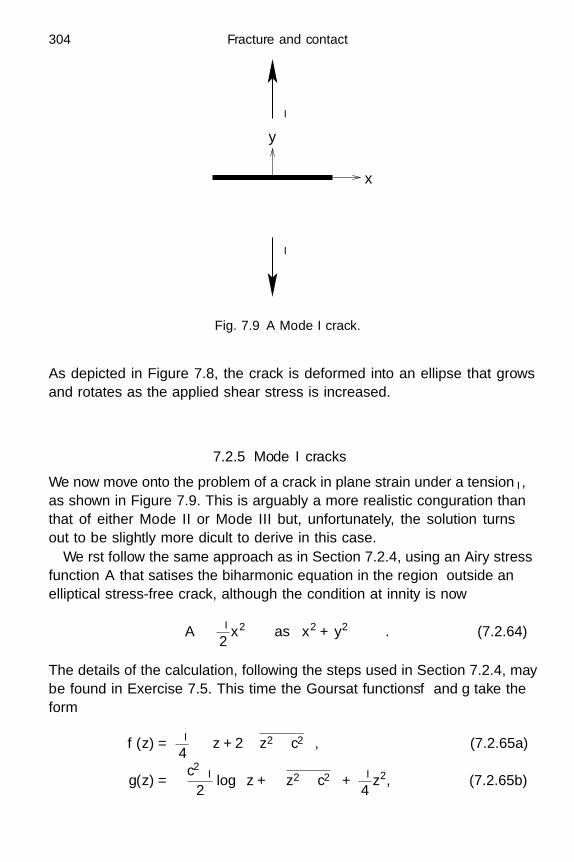
304 Fracture and contact
x
y
σI
σI
Fig. 7.9 A Mode I crack.
As depicted in Figure 7.8, the crack is deformed into an ellipse that growsand rotates as the applied shear stress is increased.
7.2.5 Mode I cracks
We now move onto the problem of a crack in plane strain under a tension σI,as shown in Figure 7.9. This is arguably a more realistic configuration thanthat of either Mode II or Mode III but, unfortunately, the solution turnsout to be slightly more difficult to derive in this case.
We first follow the same approach as in Section 7.2.4, using an Airy stressfunction A that satisfies the biharmonic equation in the region Ω outside anelliptical stress-free crack, although the condition at infinity is now
A ∼ σI
2x2 as x2 + y2 → ∞. (7.2.64)
The details of the calculation, following the steps used in Section 7.2.4, maybe found in Exercise 7.5. This time the Goursat functions f and g take theform
f(z) =σI
4
(−z + 2
√z2 − c2
), (7.2.65a)
g(z) = −c2σI
2log
(z +
√z2 − c2
)+
σI
4z2, (7.2.65b)
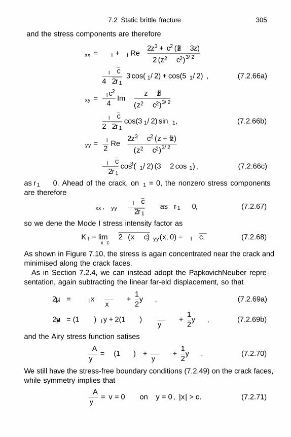
7.2 Static brittle fracture 305
and the stress components are therefore
τxx = −σI + σI Re
2z3 + c2 (z − 3z)
2 (z2 − c2)3/2
∼ σI√
c
4√
2r1
(3 cos(θ1/2) + cos(5θ1/2)
), (7.2.66a)
τxy =σIc
2
4Im
z − z
(z2 − c2)3/2
∼ σI√
c
2√
2r1cos(3θ1/2) sin θ1, (7.2.66b)
τyy =σI
2Re
2z3 − c2 (z + z)
(z2 − c2)3/2
∼ σI√
c√2r1
cos3(θ1/2) (3 − 2 cos θ1) , (7.2.66c)
as r1 → 0. Ahead of the crack, on θ1 = 0, the nonzero stress componentsare therefore
τxx, τyy ∼ σI√
c√2r1
as r1 → 0, (7.2.67)
so we define the Mode I stress intensity factor as
KI = limx↓c
√2π (x − c)τyy(x, 0) = σI
√πc. (7.2.68)
As shown in Figure 7.10, the stress is again concentrated near the crack andminimised along the crack faces.
As in Section 7.2.4, we can instead adopt the Papkovich–Neuber repre-sentation, again subtracting the linear far-field displacement, so that
2µu = −νσIx − ∂
∂x
(φ +
12yψ
), (7.2.69a)
2µv = (1 − ν)σIy + 2(1 − ν)ψ − ∂
∂y
(φ +
12yψ
), (7.2.69b)
and the Airy stress function satisfies
∂A
∂y= −(1 − ν)ψ +
∂
∂y
(φ +
12yψ
). (7.2.70)
We still have the stress-free boundary conditions (7.2.49) on the crack faces,while symmetry implies that
∂A
∂y= v = 0 on y = 0, |x| > c. (7.2.71)
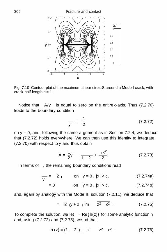
306 Fracture and contact
Fig. 7.10 Contour plot of the maximum shear stress S around a Mode I crack, withcrack half-length c = 1.
Notice that ∂A/∂y is equal to zero on the entire x-axis. Thus (7.2.70)leads to the boundary condition
∂φ
∂y=(
12− ν
)ψ (7.2.72)
on y = 0, and, following the same argument as in Section 7.2.4, we deducethat (7.2.72) holds everywhere. We can then use this identity to integrate(7.2.70) with respect to y and thus obtain
A =12yψ − φ
1 − 2ν+
σIx2
2. (7.2.73)
In terms of ψ, the remaining boundary conditions read
∂ψ
∂y= −2σI on y = 0, |x| < c, (7.2.74a)
ψ = 0 on y = 0, |x| > c, (7.2.74b)
and, again by analogy with the Mode III solution (7.2.11), we deduce that
ψ = −2σIy + 2σI Im√
z2 − c2
. (7.2.75)
To complete the solution, we let φ = Reh(z) for some analytic function h
and, using (7.2.72) and (7.2.75), we find that
h′(z) = (1 − 2ν)σI
z −
√z2 − c2
. (7.2.76)
0
0.2
0.4
0.6
0.8
1
-2 -1 0 1 2-2
-1
0
1
2
y
x
S/σI

7.2 Static brittle fracture 307
-1 -0.5 0.5 1
-0.2
-0.1
0.1
0.2
x
y
2 (1 − ν) σI/µ = 0
0.5
0.25
Fig. 7.11 The displacement of a Mode I crack of half-length c = 1 under increasingnormal stress σI .
This may be integrated to give
h(z) =(
12− ν
)σI
z2 − z
√z2 − c2 + c2 log
(z +
√z2 − c2
). (7.2.77)
By combining (7.2.73), (7.2.75) and (7.2.77), we obtain a solution for theAiry stress function analogous to the Goursat representation (7.2.65).
The displacement of the crack may now be found by evaluating (7.2.69)on y = 0±, |x| < c as
2µu = −νσIx − Reh′(z)
= −(1 − ν)σIx, (7.2.78a)
2µv = (1 − ν)ψ = ±2(1 − ν)σI
√c2 − x2. (7.2.78b)
Figure 7.11 shows that the crack becomes elliptical, growing wider andshorter as the applied normal stress increases.
We conclude this discussion with two remarks. First, we note that a gen-eral planar crack in two space dimensions will be a linear superposition ofModes I, II and III, and hence the stress near its tip will be characterisedby three intensity factors. The calculations carried out above suggest thatall three will scale with the square root of the crack length, but unfortu-nately there are no general rules about the factors to which a crack will bemost vulnerable. Second, the most famous three-dimensional crack configu-ration is the penny-shaped crack which is the radially symmetric version ofour earlier Mode I crack and it can be solved explicitly, with a great dealof effort, by transforming to spheroidal coordinates and taking a limit as inSection 7.2.2. Both these configurations, along with many others, are lucidlydescribed in Sneddon & Lowengrub (1969).

308 Fracture and contact
7.2.6 Dynamic fracture
All the discussion hitherto refers to models of cracks that are static or justabout to grow. If, however, we wish to describe structural failure or the re-sponse of tectonic plates to earthquakes, for example, we need to be ableto predict the speed of penetration of a growing crack. Unfortunately thisinvolves synthesising the theories of elastic wave propagation from Chap-ter 3 with those of mixed boundary value problems from this chapter, andthis task is beyond the scope of this book (see Freund, 1989, for a helpfulaccount).
We therefore restrict our attention to the simplest possible model fora semi-infinite Mode III crack propagating at constant speed −V along thex-axis, so its tip is at x = −V t. Although the global stress field away from thecrack will be a complicated history-dependent function of the crack geome-try, it is reasonable to assume that the local stress field may be approximatedby a travelling wave moving with speed −V , at least on sufficiently shorttime-scales. Hence, the local displacement will satisfy(
1 − V 2
c2s
)∂2w
∂ξ2 +∂2w
∂y2 = 0 (7.2.79a)
everywhere except on y = 0, ξ > 0, with
µ∂w
∂y= 0 on y = 0, ξ > 0, (7.2.79b)
where ξ = x + V t and cs is the shear wave speed. Notice that this problemgeneralises the static semi-infinite Mode III crack problem considered in(7.2.3).
To close the model (7.2.79), we should impose some conditions at infinity,but this would require us to solve for the stress away from the crack. Evenwithout precise knowledge of this far field, we expect the physically relevantsolution to have a square root singularity analogous to (7.2.4) with n = 1.The corresponding solution of (7.2.79) is
w = A Re
(√ξ
B+ iy
), where B2 = 1 − V 2
c2s
, (7.2.80)
and it is only through the constant A that the global stress field is felt. Nowthe dynamic stress intensity factor is
KIII = µ√
2π limξ↑0
(√−ξ
∂w
∂y(ξ, 0)
)= µA
√πB
2= µA
√π
2
(1 − V 2
c2s
)1/4
.
(7.2.81)
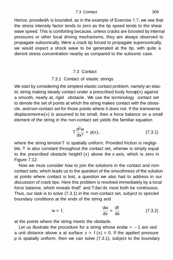
7.3 Contact 309
Hence, provided A is bounded, as in the example of Exercise 7.7, we see thatthe stress intensity factor tends to zero as the tip speed tends to the shearwave speed. This is comforting because, unless cracks are boosted by internalpressures or other local driving mechanisms, they are always observed topropagate subsonically. Were a crack tip forced to propagate supersonically,we would expect a shock wave to be generated at the tip, with quite adifferent stress concentration nearby as compared to the subsonic case.
7.3 Contact
7.3.1 Contact of elastic strings
We start by considering the simplest elastic contact problem, namely an elas-tic string making steady contact under a prescribed body force p(x) againsta smooth, nearly flat, rigid obstacle Γ. We use the terminology contact setto denote the set of points at which the string makes contact with the obsta-cle, and non-contact set for those points where it does not. If the transversedisplacement w(x) is assumed to be small, then a force balance on a smallelement of the string in the non-contact set yields the familiar equation
Td2w
dx2 = p(x), (7.3.1)
where the string tension T is spatially uniform. Provided friction is negligi-ble, T is also constant throughout the contact set, where w is simply equalto the prescribed obstacle height f(x) above the x-axis, which is zero inFigure 7.12.
Now we must consider how to join the solutions in the contact and non-contact sets, which leads us to the question of the smoothness of the solutionat points where contact is lost, a question we also had to address in ourdiscussion of crack tips. Here this problem is resolved immediately by a localforce balance, which reveals that T and Tdw/dx must both be continuous.Thus, our task is to solve (7.3.1) in the non-contact set, subject to specifiedboundary conditions at the ends of the string and
w = f,dw
dx=
df
dx(7.3.2)
at the points where the string meets the obstacle.Let us illustrate the procedure for a string whose ends x = ±1 are fixed
a unit distance above a flat surface z = f(x) = 0. If the applied pressurep is spatially uniform, then we can solve (7.3.1), subject to the boundary

310 Fracture and contact
1.0 0.5 0.5 1.0
0.2
0.4
0.6
0.8
1.0
w
x
increasing p
Fig. 7.12 Solution for the contact between a string and a level surface, with appliedpressure p/T = 0, 1, 2, 3, 4, 5.
conditions w(−1) = w(1) = 1, to obtain
w = 1 − p
2T
(1 − x2) . (7.3.3)
As the applied pressure p is increased, the downward displacement at thecentre of the string increases, until it first makes contact with z = 0 whenp = 2T .
If the pressure is increased further, then a contact set forms near themiddle of the string. Let us denote the boundaries of this region by x = ±s,where s is to be determined as part of the solution. In this simple problem, weonly need to solve for positive x; the solution in x < 0 may then be inferredby symmetry. We therefore solve (7.3.1) in x > s, subject to w(1) = 1 andthe continuity conditions
w(s) =dw
dx(s) = 0 (7.3.4)
to obtain
w = 1 − p
2T(1 − x)(1 + x − 2s) (7.3.5)
in x > s, where
s = 1 −√
2T
p. (7.3.6)
In Figure 7.12 we see how, as increasing pressure is applied, the string ispushed downward, makes contact with the surface beneath, and the contactset then gradually spreads outwards.
This simple example shows how the solution of the contact problem hingeson locating the free boundary between the contact and non-contact sets.

7.3 Contact 311
1.0 0.5 0.5 1.0
0.05
0.10
0.15
0.20
0.25
0.30
1.0 0.5 0.5 1.0
0.05
0.10
0.15
0.20
0.25
0.30
1.0 0.5 0.5 1.0
0.05
0.10
0.15
0.20
0.25
0.30
(a) (b) (c)z z z
x x x
Fig. 7.13 Three candidate solutions for the contact problem between a stress-freestring and the surface z = 2x2 − 3x4 .
Such free boundary problems are inevitably nonlinear even when, as in(7.3.1), the governing equation is itself linear. This means that the solu-tions of contact problems can exhibit phenomena such as non-uniquenessthat are impossible for linear problems.
To illustrate some of the possible pitfalls, consider now a string, subjectto zero body force, stretched over the curved surface
z = f(x) = 2x2 − 3x4 (7.3.7)
with its ends fixed at w(−1) = w(1) = 0. With p = 0, (7.3.1) implies thatthe string must be straight wherever it is out of contact. The most obviouslinear function satisfying both boundary conditions is simply w ≡ 0 but, ascan be seen in Figure 7.13(a), this would imply that the string penetratesthe obstacle, which is impossible. We must therefore allow the string to makecontact with the obstacle, as illustrated in Figure 7.13(b). Recalling that thestring must meet the obstacle tangentially, the solution in this case is easilyconstructed as
w =
89(1 + x), −1 x −2
3,
2x2 − 3x4, −23
x 23,
89(1 − x),
23
x 1.
(7.3.8)
We can, however, construct a third solution, shown in Figure 7.13(c), inwhich the string loses contact with the middle of the obstacle. Again notingthat the string is linear when out of contact and must always make contact

312 Fracture and contact
tangentially, we find that this solution takes the form
w =
89(1 + x), −1 x −2
3,
2x2 − 3x4, −23
x − 1√3,
13, − 1√
3 x 1√
3,
2x2 − 3x4,1√3
x 23,
89(1 − x),
23
x 1.
(7.3.9)
We would like to have a mathematical formulation that chooses betweenpossible candidate solutions like those shown in Figure 7.13. The situationshown in Figure 7.13(a) can be avoided by incorporating the requirementw f into our model. Although it is slightly less obvious, Figure 7.13(b)is also physically unrealistic, since there is a tensile normal stress betweenthe string and the obstacle. In general, if R(x) denotes the normal reactionforce exerted on the string by the obstacle, then (7.3.1) is modified to
Td2w
dx2 = p − R. (7.3.10)
The reaction force R must be zero outside the contact set. The solutionshown in Figure 7.13(b) has negative values of R and is therefore unphysical;the correct solution is therefore (7.3.9).
To summarise, we can select a physically relevant solution of the contactproblem by insisting that
w = f, Td2w
dx2 − p < 0 in the contact set, (7.3.11a)
and
w > f, Td2w
dx2 − p = 0 in the non-contact set, (7.3.11b)
with continuity of w and dw/dx at the boundaries between the contact andnon-contact sets. The two conditions (7.3.11) may usefully be combined to
(w − f)(
Td2w
dx2 − p
)= 0, with w f, T
d2w
dx2 − p 0, (7.3.12)
and this so-called linear complementarity problem can be written in anotherway which is very convenient computationally.
7.3 Contact 313
If w satisfies
T
∫ 1
−1
dw
dx
(dv
dx− dw
dx
)dx
∫ 1
−1p(w − v) dx for all v f, (7.3.13)
with v and w satisfying the same fixed boundary conditions, then, as shownin Elliott & Ockendon (1982, p. 103), w satisfies (7.3.12). The statement(7.3.13) is called a variational inequality, and, as shown in Exercise 7.8, w
satisfies (7.3.13) if and only if it is the minimiser of the functional∫ 1
−1
T
2
(dv
dx
)2
+ pv
dx
over all v f . This has the obvious physical interpretation of minimisingthe elastic energy minus the work done by pressure over the virtual dis-placements v which prevent inter-penetration of the string and the obstacle.Moreover, this constrained optimisation problem is very much easier to solvenumerically than the free boundary problem (7.3.1), (7.3.2).
7.3.2 Other thin solids
It is seemingly straightforward to extend the model derived above to describesmooth contact between an elastic beam and a rigid substrate. In the non-contact set, the displacement w of the beam is governed by the equation
Td2w
dx2 − EId4w
dx4 − p = 0, (7.3.14)
where, as in Chapter 4, EI denotes the bending stiffness. Evidently (7.3.14)reduces to (7.3.1) as the bending stiffness tends to zero. In the contact set,(7.3.14) is simply replaced by the condition w = f .
Since (7.3.14) is fourth-order, we expect to need additional boundary con-ditions to specify a unique solution. Now, by balancing forces and momentsat the boundary between the contact and non-contact sets, we deduce thatw, dw/dx and d2w/dx2 must all be continuous there.
Let us illustrate the solution procedure in this case by considering a beamthat is simply supported at its two ends x = ±1 at a unit height above thehorizontal surface z = 0. This is the equivalent for a beam of the stringsagging problem analysed in Section 7.3.1, and we will see that the inclusionof bending stiffness leads to interesting new behaviour.
Assuming no tension is applied, (7.3.14) reduces to
d4w
dx4 = − p
EI, (7.3.15)

314 Fracture and contact
1.0 0.5 0.5 1.0
0.2
0.4
0.6
0.8
1.0
1.0 0.5 0.5 1.0
0.2
0.4
0.6
0.8
1.0
1.0 0.5 0.5 1.0
0.2
0.4
0.6
0.8
1.0
x
w w w
x x
(a) (b) (c)
Fig. 7.14 The contact between a beam and a horizontal surface under a uniformpressure p. (a) The beam sags towards the surface: p/EI = 0, 12/5, 24/5. (b) Thebeam makes contact at just one point: p/EI = 24/5, 24. (c) The contact set grows:p/EI = 24, 2048/27, 384.
subject to the boundary conditions
w(−1) = 1,d2w
dx2 (−1) = 0, (7.3.16a)
w(1) = 1,d2w
dx2 (1) = 0, (7.3.16b)
and this problem is easily solved to give the displacement
w = 1 − p
24EI
(1 − x2) (5 − x2) . (7.3.17)
As shown in Figure 7.14(a), the beam sags under increasing applied pressureuntil it first makes contact with the surface z = 0 when p/EI = 24/5.
The solution (7.3.17) cannot remain valid for p/EI > 24/5, because itpredicts negative values of w. So, let us instead seek a solution in whichthe beam makes contact with z = 0 over a region −s x s. We needonly solve the problem in x > 0, since we can then infer the solution fornegative values of x by symmetry. We therefore replace (7.3.16a) with thefree boundary conditions
w(s) = 0,dw
dx(s) = 0,
d2w
dx2 (s) = 0. (7.3.16c)
Notice again that, compared with (7.3.16a), we have introduced one moreboundary condition to compensate for not knowing the location of the freeboundary a priori. Again, the problem is easy to solve and we find that
w =(x − s)3(2 − s − x)
(1 − s)4 (7.3.18a)
in x s, with w ≡ 0 in 0 x s, where s is related to the applied

7.3 Contact 315
pressure by
p
EI=
24(1 − s)4 or s = 1 −
(24EI
p
)1/4
. (7.3.18b)
In Figure 7.14(c) we show how the contact set grows as p increases, withs = 0, 1/4, 1/2 when p/EI = 24, 2048/27, 384 respectively. However, since s
must lie between 0 and 1, the solution (7.3.18) is only valid when p/EI 24.This begs the question: “what happens for values of p/EI between 24/5and 24?” The answer is that the beam makes contact at just one point,namely the origin. If we replace (7.3.16c) with
w(0) = 0,dw
dx(0) = 0, (7.3.16d)
then we find
w =x2(3 − x)
2− p
48EIx2(1 − x)(3 − 2x), (7.3.19)
in x 0, with the even extension of (7.3.19) in x 0. As shown in Fig-ure 7.14(b), the beam initially meets z = 0 at one point, then flattens asp increases, until its curvature matches the curvature of the obstacle. Onlythen does the contact set start to grow. It is easy to verify that (7.3.19)matches (7.3.17) and (7.3.18) when p/EI = 24/5 and 24 respectively.
The final surprise comes when we consider the reaction force R exertedby the surface z = 0 on the beam, given by
R = p + EId4w
dx4 . (7.3.20)
Consider first the solution (7.3.19) in which the contact set is the pointx = 0. By differentiating (7.3.19) and using the symmetry about x = 0, wefind that
d3w
dx3 (0+) = −d3w
dx3 (0−) =5p
8EI− 3. (7.3.21)
Hence the third derivative of w is discontinuous across x = 0 and (7.3.20)then implies that there is a delta-function in the reaction force:
R =(
5p
4− 6EI
)δ(x). (7.3.22)
Similarly, differentiation of (7.3.18) reveals that
d3w
dx3 (s+) =12
(1 − s)3 =(
32
)1/4 ( p
EI
)3/4, (7.3.23)
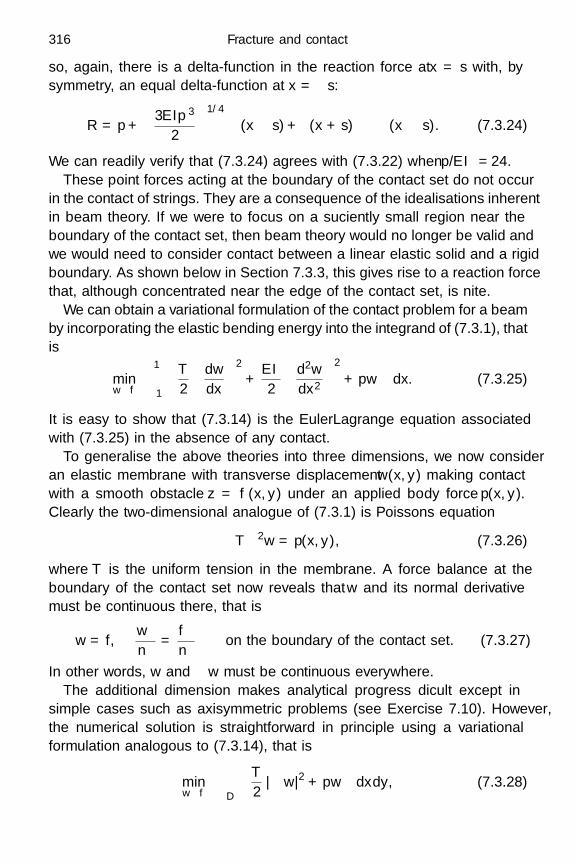
316 Fracture and contact
so, again, there is a delta-function in the reaction force at x = s with, bysymmetry, an equal delta-function at x = −s:
R = p +(
3EIp3
2
)1/4 (δ(x − s) + δ(x + s)
)(x s). (7.3.24)
We can readily verify that (7.3.24) agrees with (7.3.22) when p/EI = 24.These point forces acting at the boundary of the contact set do not occur
in the contact of strings. They are a consequence of the idealisations inherentin beam theory. If we were to focus on a sufficiently small region near theboundary of the contact set, then beam theory would no longer be valid andwe would need to consider contact between a linear elastic solid and a rigidboundary. As shown below in Section 7.3.3, this gives rise to a reaction forcethat, although concentrated near the edge of the contact set, is finite.
We can obtain a variational formulation of the contact problem for a beamby incorporating the elastic bending energy into the integrand of (7.3.1), thatis
minwf
∫ 1
−1
T
2
(dw
dx
)2
+EI
2
(d2w
dx2
)2
+ pw
dx. (7.3.25)
It is easy to show that (7.3.14) is the Euler–Lagrange equation associatedwith (7.3.25) in the absence of any contact.
To generalise the above theories into three dimensions, we now consideran elastic membrane with transverse displacement w(x, y) making contactwith a smooth obstacle z = f(x, y) under an applied body force p(x, y).Clearly the two-dimensional analogue of (7.3.1) is Poisson’s equation
T∇2w = p(x, y), (7.3.26)
where T is the uniform tension in the membrane. A force balance at theboundary of the contact set now reveals that w and its normal derivativemust be continuous there, that is
w = f,∂w
∂n=
∂f
∂non the boundary of the contact set. (7.3.27)
In other words, w and ∇w must be continuous everywhere.The additional dimension makes analytical progress difficult except in
simple cases such as axisymmetric problems (see Exercise 7.10). However,the numerical solution is straightforward in principle using a variationalformulation analogous to (7.3.14), that is
minwf
∫∫D
(T
2|∇w|2 + pw
)dxdy, (7.3.28)

7.3 Contact 317
δ
f(x) c
punch
x
y
Fig. 7.15 Contact between a rigid body and an elastic half-space.
and we can additionally incorporate bending stiffness as follows:
minwf
∫∫D
(T
2|∇w|2 +
EI
2(∇2w
)2 + pw
)dxdy. (7.3.29)
7.3.3 Smooth contact in plane strain
As an intermediate case between the thin contact problems described aboveand general three-dimensional elastic contact, we will now make some ele-mentary observations about contact in plane strain. For simplicity, we limitour attention to the problem of a rigid body, known as a punch, pushed adistance δ into the elastic half-space y > 0, as shown in Figure 7.15.
Let us suppose the geometry is symmetric about x = 0 so that the con-tact set is −c < x < c for some positive c. Inside this region, the normaldisplacement is given in terms of the shape f(x) of the punch and, assumingsmooth contact, the tangential stress is zero. In addition, there must be apositive reaction force, so that
v = δ − f(x), τxy = 0, τyy < 0 on y = 0, |x| < c. (7.3.30a)
Outside the contact set, the surface traction is zero and there must be nointer-penetration, that is
τxy = τyy = 0, v > δ − f(x) on y = 0, |x| > c. (7.3.30b)
Our task, then, is to solve plane strain subject to the mixed boundaryconditions (7.3.30) on y = 0 and given behaviour, typically zero stress, at

318 Fracture and contact
infinity. Such problems are almost always so complicated that they must besolved computationally but, enlightened by (7.3.14), we can see that this isnot as fearsome a task as might be supposed. One must devise a code thatminimises the integral ∫∫
y>0W dxdy,
where W is the strain energy density defined in Section 1.9, over all dis-placement fields satisfying the constraint v(x, 0) f(x) − δ. The proof ofthe equivalence of this proposed algorithm to finding a displacement fieldsatisfying the Navier equation and the boundary conditions (7.3.30) reliescrucially on the fact that the boundary conditions together with the inequal-ities in (7.3.30) determine a unique solution with bounded stress everywhere.
One cunning way to construct analytic solutions of the contact problemdescribed above is to suppose that we know in advance both the size c ofthe contact set and the contact pressure, say p(x), exerted by the punch.We thus replace the boundary conditions (7.3.30) with
τxy = 0, τyy = −P (x) on y = 0, (7.3.31)
where
P (x) =
p(x), |x| < c,
0, |x| > c.(7.3.32)
We can now use the solution obtained in (2.6.85) to calculate the displace-ment v0(x) of the boundary y = 0, given by
v0(x) = −1 − ν
πµ
∫ c
−cp(s) log |s − x|ds. (7.3.33)
In |x| < c, this allows us to recover the shape of the punch that correspondsto the assumed pressure profile p(x). It only remains to check for consistencythat there is no inter-penetration in |x| > c.
As an example (guided by hindsight), let us consider the pressure profile
p(x) = F√
c2 − x2, (7.3.34)
where F is constant. By calculating the integral in (7.3.33) for this particular
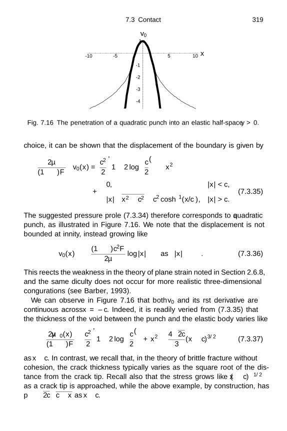
7.3 Contact 319
-10 -5 5 10
-4
-3
-2
-1
1
x
v0
Fig. 7.16 The penetration of a quadratic punch into an elastic half-space y > 0.
choice, it can be shown that the displacement of the boundary is given by(2µ
(1 − ν)F
)v0(x) =
c2
2
[1 − 2 log
( c
2
)]− x2
+
0, |x| < c,
|x|√
x2 − c2 − c2 cosh−1(x/c), |x| > c.(7.3.35)
The suggested pressure profile (7.3.34) therefore corresponds to a quadraticpunch, as illustrated in Figure 7.16. We note that the displacement is notbounded at infinity, instead growing like
v0(x) ∼ −(1 − ν)c2F
2µlog |x| as |x| → ∞. (7.3.36)
This reflects the weakness in the theory of plane strain noted in Section 2.6.8,and the same difficulty does not occur for more realistic three-dimensionalconfigurations (see Barber, 1993).
We can observe in Figure 7.16 that both v0 and its first derivative arecontinuous across x = ±c. Indeed, it is readily verified from (7.3.35) thatthe thickness of the void between the punch and the elastic body varies like
2µv0(x)(1 − ν)F
− c2
2
[1 − 2 log
( c
2
)]+ x2 ∼ 4
√2c
3(x − c)3/2 (7.3.37)
as x ↓ c. In contrast, we recall that, in the theory of brittle fracture withoutcohesion, the crack thickness typically varies as the square root of the dis-tance from the crack tip. Recall also that the stress grows like (x − c)−1/2
as a crack tip is approached, while the above example, by construction, hasp ∼
√2c√
c − x as x ↑ c.
320 Fracture and contact
These observations prompt the question: “why should the stress singu-larity in the smooth contact problem be weaker than that in the fractureproblem?” The answer lies in the fact that the crack geometry is prescribeda priori; it is perfectly sensible to seek the stress distributions around acrack with arbitrary faces and an arbitrary crack tip surrounding these faces.However the boundary of a smooth contact set is free to decide its location,and it does so in such a way as to prevent the stress intensification that ischaracteristic of fracture. Notice also that the introduction of cohesion intothe tip region of a brittle crack, as shown in Exercise 7.3, can also reducethe strength of the singularity to a 3/2-power as in (7.3.37), when weregard the cohesion length as a free parameter.
7.4 Concluding remarks
The role of friction is of great importance in most real contact problems,but thus far we have not mentioned it. This is because of the serious math-ematical complications to which it leads. Suppose for example we introducefrictional effects into the smooth contact problems of Section 7.3. If we as-sume Coulomb friction, then the shear stress |τxy | at the contact set neverexceeds the normal stress |τyy | multiplied by the coefficient of friction, µc.This immediately introduces a second component into the free boundary; onecomponent separates the non-contact set from the contact set, and the otherdivides the contact set into regions where |τxy | < µc|τyy | and |τxy | = µc|τyy |respectively. In the former there is no slip, so the displacement is continuous;but in the latter, slip is possible, and only the normal displacement is con-tinuous. This considerable extra complexity destroys any hope of applyingthe standard theory of variational inequalities.
Unfortunately, theoretical challenges of this sort have to be confronted ifwe are addressing even the apparently simple problem of finding the forcesexerted on the ends of a rigid ladder resting against a wall. This is a nontriv-ial problem unless limiting friction is assumed at both ends of the ladder. Asis usual in frictional contact, without this assumption, the reaction forcesare indeterminate, and the only way forward is to consider the geometryof the ends of the ladder in detail, and solve a frictional contact problemalong the lines just described. The ladder will be ready to slip when theslipping subset of the contact region is found to occupy almost the whole ofthe contact region.
Strictly speaking, the ladder problem should be solved as an evolutioncontact problem starting from the time at which the ladder was erected.Such dynamic contact problems are of greatest applicability in the theory of
Exercises 321
impact, where predictions are to be made of, say, coefficients of restitutionbetween various different solids. To carry this out, even in the non-frictionalcase, requires a combination of the modelling in this chapter and of theelastic waves in Chapter 3.
One frictional contact problem of great practical importance which canbe solved exactly is the capstan problem, in which a rope is wound arounda rough circular cylinder. In polar coordinates, we suppose that the tensionin the rope is T (θ) and that the cylinder is given by r = a. Making theassumption of limiting Coulomb friction everywhere, (7.3.1) implies that thenormal reaction of the capstan is T (θ)/a, and a force balance equation alongthe rope gives dT/dθ = µcT , where µc is again the coefficient of friction.The resulting exponential dependence of T on θ explains the effectivenessof capstans. Moreover, this kind of configuration can be used as a buildingblock in a theory of knots (real, not mathematical, ones!).
Exercises
7.1 For the elliptical Mode III crack solution (7.2.9), show that the stresscomponents on y = 0, x > c cosh ε are given by
τxz = 0, τyz = 2τ0eε
(x cosh ε√x2 − c2
− sinh ε
).
Deduce that the stress at the crack tip is
τyz = 2τ0eε cosech ε ∼ 2τ0
εas ε → 0.
Show also that the radius of curvature r0 of the tip is given by
1r0
=cosh ε
c sinh2 ε∼ 1
ε2c
and hence that the shear stress at the tip is approximately
τyz ∼ 2τ0
√c
r0
when r0 is small.7.2 Show that the right-hand side of (7.2.18) tends to σIII
√c2 − x2 as
y ↓ 0 when |x| < c. Show also that, as y ↓ 0,
∂
∂y
∫ c
−cf(ξ) tan−1
(x − ξ
y
)dξ → −
∫ c
−c
f(ξ) dξ
ξ − x,

322 Fracture and contact
where −∫
denotes the principal value integral defined in Exercise 2.12.Deduce that a solution of the singular integral equation
−∫ c
−c
f(ξ) dξ
ξ − x= 1 (|x| < c)
is f(ξ) = ξ/(π√
c2 − ξ2). Are there any others?
7.3 Consider a semi-infinite planar Mode III crack along the positivex-axis with a cohesive stress C in a neighbourhood of the cracktip. The antiplane displacement w(x, y) satisfies Laplace’s equationoutside the crack, subject to the boundary conditions
w(x, 0) = 0, x < 0, µ∂w
∂y(x, 0) =
C, 0 < x < δ,
0, x > δ,
and the far-field condition
w ∼√
2π
K
µRe
(√z)
as x2 + y2 → ∞,
where z = x + iy and K is a constant determined by the externalstress imposed on the crack.
Show that the coordinate transformation (x+iy) = (ξ +iη)2 leadsto the chain rule
∂
∂y=
12 (ξ2 + η2)
(η
∂
∂ξ+ ξ
∂
∂η
).
Deduce that w is a harmonic function of (ξ, η) in η > 0 satisfying
µ∂w
∂η(ξ, 0) =
2Cξ, |ξ| <
√δ,
0, |ξ| >√
δ,
and
w ∼√
2π
K
µξ as η → ∞.
Verify that the solution for ∂w/∂η is
∂w
∂η=
2C
πµIm
ζ log
(ζ −
√δ
ζ +√
δ
),
where ζ = ξ + iη, and deduce that
∂w
∂ξ=
2C
πµRe
ζ log
(ζ +
√δ
ζ −√
δ
)− 2
√δ
+
√2π
K
µ.
Exercises 323
Hence show that the stress ahead of the crack is given by
µ∂w
∂y(x, 0) =
(K√2π
− 2C√
δ
π
)1√−x
+ C
[1 − 2
πtan−1
(√−x
δ
)]in x < 0, and deduce that the stress at the crack tip is finite if
δ =πK2
8C2 .
7.4 By writing the Airy stress function in the form (7.2.24) and usingthe chain rules (7.2.42), show that the stress components in planestrain are given in terms of the Goursat functions by
∂2A
∂x2 = Rezf ′′(z) + 2f ′(z) + g′′(z)
,
∂2A
∂y2 = Re−zf ′′(z) + 2f ′(z) − g′′(z)
,
− ∂2A
∂x∂y= Im
zf ′′(z) + g′′(z)
.
7.5 Apply the conformal mapping technique from Section 7.2.4 to aMode I crack. Show that the far-field condition (7.2.64) correspondsto f ∼ σIz/4 and g ∼ σIz
2/4 as z → ∞, and that (7.2.35) becomes
− F (1/ζ) − σI(a + 2b)4ζ
+σIbζ
4
=ζ2G′(ζ) + ζ
(a + bζ2
)F ′(ζ)
aζ2 − b− σI(a + 2b)
4ζ+
σIbζ
4.
In the limit a, b → c/2, deduce that F and G are given up to arbitraryintegration constants by
F (ζ) =cσI
8
(1ζ− 3ζ
),
G(ζ) =c2σI
16
(ζ +
1ζ
)− c2σI
2log
(c
ζ
).
By inverting the conformal mapping, obtain (7.2.65).7.6 Show that the displacement components and the Airy stress function
in plane strain are related by
2(λ + µ)(
∂u
∂x+
∂v
∂y
)= ∇2A,
324 Fracture and contact
and deduce that there exists a function ψ(x, y) such that
u =1
2(λ + µ)∂A
∂x+
∂ψ
∂y, v =
12(λ + µ)
∂A
∂y− ∂ψ
∂x.
By eliminating u and v from the constitutive relations, show that A
and ψ satisfy
∂2A
∂x2 − ∂2A
∂y2 = − 2µ
1 − ν
∂2ψ
∂x∂y,
2∂2A
∂x∂y=
µ
1 − ν
(∂2ψ
∂x2 − ∂2ψ
∂y2
).
Deduce that∂2
∂z2
(A − µ
1 − νiψ)
= 0,
where z = x + iy and z = x − iy, and hence that
A − µ
1 − νiψ = zf(z) + g(z),
where f and g are arbitrary analytic functions.Hence show that the displacement components are given in terms
of f and g by
u + iv =12µ
((3 − 4ν)f(z) − zf ′(z) − g′(z)
).
Recalling the boundary condition (7.2.26) satisfied by f and g on astress-free boundary, show that the displacement of such a boundaryis given by
u + iv =2 (1 − ν)
µf(z).
Finally, use the expression (7.2.65a) for f(z) to reproduce the dis-placement (7.2.78) of a Mode I crack.
7.7 Suppose a semi-infinite Mode III crack propagates at constant speed−V along the x-axis in a channel |y| < h, −∞ < x < ∞, so thatthe displacement w satisfies (7.2.79). Suppose also that antiplaneshear displacements are applied on the walls of the channel suchthat w = ±b on y = ±h, respectively. Deduce that
∂2w
∂X2 +∂w
∂y= 0,

Exercises 325
where x + V t = ξ =(1 − V 2/c2
s
)1/2X, and verify that the solution
is
w =by
h− b
πIm
log
(1 +
√1 − eπz/h
),
where z = X+iy. [Alternatively, obtain this result by using conformalmapping.]
Hence show that∂w
∂y(x, 0) ∼ b
2√
πh
1√−X
as X ↑ 0, and deduce that the propagation speed is given by
V = cs
√1 − K4
IIIh2
µ4b4 ,
where KIII is the Mode III stress intensity factor.7.8 (a) Show that, if
U [w] =∫ 1
−1
(T
2
(dw
dx
)2
+ pw
)dx,
then
U [w] − U [v] =∫ 1
−1p (w − v) dx
− T
∫ 1
−1
dw
dx
(dv
dx− dw
dx
)dx − T
2
∫ 1
−1
(dw
dx− dv
dx
)2
dx
and deduce that, if w satisfies (7.3.13), then it minimises U .(b) Note that, if v1 and v2 belong to the set v : v f on (−1, 1),
then so does αv1 + (1 − α)v2 for 0 < α < 1 [this means thatthe set is convex]. Show that if w minimises U , then
U [w] U [αv + (1 − α)w]
for all v f . Expand this inequality for small α to show that
0 ∫ 1
−1
(T
dw
dx
(dv
dx− dw
dx
)− p(w − v)
)dx.
7.9 Consider the problem of a flexible ruler of unit length being pressedagainst a horizontal table, as shown in Figure 7.17. Suppose the endx = 0 is simply supported by the table with w = 0, while a bendingmoment M is applied at the other end, x = 1, which is held at a
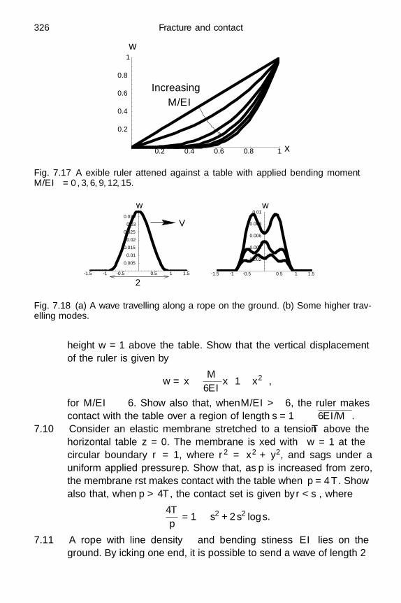
326 Fracture and contact
0.2 0.4 0.6 0.8 1
0.2
0.4
0.6
0.8
1
w
x
Increasing
M/EI
Fig. 7.17 A flexible ruler flattened against a table with applied bending momentM/EI = 0, 3, 6, 9, 12, 15.
-1.5 -1 -0.5 0.5 1 1.5
0.005
0.01
0.015
0.02
0.025
0.03
0.035
-1.5 -1 -0.5 0.5 1 1.5
0.002
0.004
0.006
0.008
0.01ww
η η
2
V
Fig. 7.18 (a) A wave travelling along a rope on the ground. (b) Some higher trav-elling modes.
height w = 1 above the table. Show that the vertical displacementof the ruler is given by
w = x − M
6EIx(1 − x2) ,
for M/EI 6. Show also that, when M/EI > 6, the ruler makescontact with the table over a region of length s = 1 −
√6EI/M .
7.10 Consider an elastic membrane stretched to a tension T above thehorizontal table z = 0. The membrane is fixed with w = 1 at thecircular boundary r = 1, where r2 = x2 + y2, and sags under auniform applied pressure p. Show that, as p is increased from zero,the membrane first makes contact with the table when p = 4T . Showalso that, when p > 4T , the contact set is given by r < s, where
4T
p= 1 − s2 + 2s2 log s.
7.11 A rope with line density and bending stiffness EI lies on theground. By flicking one end, it is possible to send a wave of length 2

Exercises 327
travelling along the rope at speed V , as illustrated in Figure 7.18(a).Defining the travelling wave coordinate η = x − V t, show that thesmall transverse displacement w(η) of the rope satisfies
EId4w
dη4 + V 2 d2w
dη2 + g = 0,
subject to the contact conditions
w =dw
dη=
d2w
dη2 = 0 at η = ±.
Derive the equation
w =g4
2EIk4
(2 + k2)− k2η2
2 − 2 sec k cos(
kη
)for the shape of the hump in the rope, and show that the speed isgiven by
V =k
√EI
,
where k satisfies the transcendental equation
tan k = k.
[This equation has a countably infinite set of solutions; the displace-ment corresponding to the first is shown in Figure 7.18(a) and thenext three are shown in Figure 7.18(b).]
Given that the lowest positive root is given by k1 ≈ 9/2, deducethat flicking one end of the rope up and down over a time τ willproduce a wave travelling at speed
V ≈ 3(
EI
τ 2
)1/4
.
8
Plasticity
8.1 Introduction
It is unfortunate that what are colloquially called “plastics” are polymericsolids that usually behave elastically at room temperature and viscoelas-tically when hot; hence the word plasticity should not be thought of asapplying just to such materials. Indeed, some of the most important exam-ples of plastic behaviour occur in metals. A convenient way to gain someintuition about this phenomenon is to apply an increasing bending momentto a paper clip. There is always a critical bending moment above whichthe clip fails to revert to its initial state, which means that it has becomeinelastic. This observation is encapsulated in Figure 8.1, which shows thequalitative stress/strain curve for a metal that yields when some norm of thestress tensor reaches the yield stress τY. If a stress lower than τY is applied,the material responds elastically (although possibly nonlinearly), returningto its original state when the loading is removed. However, when a stressgreater than τY is applied and then removed, a nonzero permanent strainremains.
Macroscopic plasticity modelling thus poses two key challenges. The firstis to explain the existence of a critical yield stress, above which a solid ceasesto behave elastically, and the second is to predict the irreversible behaviourthat occurs at a stress equal to or greater than this critical value. The partof the loading curve in Figure 8.1(b) above the dotted line is where thematerial is said to be undergoing work hardening.
A limiting case of the behaviour depicted in Figure 8.1, which has provedextremely useful in practical models of plastic behaviour, is known as per-fect plasticity. In perfectly plastic theories, the stress is never allowed to ex-ceed the yield stress, and the material can thus exist in one of two distinctstates. Below the yield stress, it behaves as an elastic solid and is describedby the models presented previously in this book; at and only at the yield
328

8.1 Introduction 329
stress
τY
strain strain
stress
τY
(a) (b)
unloading
loading
loading
unloading
Fig. 8.1 A typical stress–strain relationship for a plastic material: (a) below theyield stress τY ; (b) when the yield stress is exceeded.
stress, the material becomes plastic and starts to flow irreversibly. Hencethe stress–strain relationship of a perfectly plastic material is as sketchedin Figure 8.2(a): we can view this as an idealised version of Figure 8.1(a).We will see below that such models arise naturally in describing granularmaterials and metal plasticity.
It is natural to use the word “flow” to describe the permanent deforma-tion that occurs at the yield stress, although, in Chapter 1, we specificallystated that a solid does not flow in response to a stress. A yielding plasticmaterial therefore ceases to be a solid according to the definitions givenin Chapter 1. The situation is further complicated by the existence of vis-coelastic materials which behave like elastic solids in some situations andlike viscous liquids in others, as we will describe in Section 9.2. In fact, thereexist materials with ever more complicated mechanical properties that maybe characterised as “elastic-plastic”, “visco-plastic”, “elasto-visco-plastic”and so forth. The mathematical models that emerge in each case may bequite different from each other, and they all differ markedly from those usedin classical fluid mechanics in one crucial respect. While the behaviour of aclassical inviscid or Newtonian fluid is determined completely by its instan-taneous velocity field, plastic and viscoelastic materials all exhibit history-dependence, in which the behaviour at any time depends on the entire strainhistory that it has so far experienced. This can be anticipated by returningto your paper clip and cycling the stress so that it loads and unloads aboveand below τY until it eventually fractures; a typical stress–strain trajectoryis shown schematically in Figure 8.2(b).
We will spend most of this chapter describing plastic behaviour in metals.However, we will see that the small-scale behaviour underlying Figure 8.2 canonly be discerned using very-high magnification microscopes. We therefore

330 Plasticity
load
ing
unlo
adin
g
load
ing
unlo
adin
g
strain
stress
τY
strain
stress
τY
(a) (b)
Fig. 8.2 The stress–strain relationship for a perfectly plastic material: (a) under asingle loading; (b) under periodic loading/unloading.
start with a brief discussion of plastic flow in granular solids, whose small-scale behaviour is more familiar from everyday experience.
8.2 Models for granular material
8.2.1 Static behaviour
The mechanics of granular solids is of wide importance, for example inthe transport of powders, foodstuffs and coal and in understanding the be-haviour of sand dunes. Let us first consider a single particle at the surfaceof a granular solid, for example a pile of sugar on a spoon. In addition toits own weight W , the particle experiences a normal reaction force R andtangential frictional force F exerted by the pile underneath, as illustrated inFigure 8.3. We recall from Chapter 7 that R must be non-negative; indeed,it is an everyday observation that dry granular material cannot withstandany tensile stress (in the absence of any additional physical effects, such asmoisture-induced cohesion or electrostatic charges). Coulomb’s law of fric-tion is an empirical law which states that |F | R tan φ, where the materialparameter φ is called the angle of friction. (In the notation of Section 7.4,tan φ = µc, where µc is the coefficient of friction.) In addition, Coulomb’slaw implies that the particle is held in place by friction if |F | < R tan φ andcan slide only when |F | = R tan φ. A force balance on the particle illustratedin Figure 8.3 gives R = W cos θ and F = W sin θ, where θ is the angle thatthe surface makes with the horizontal. From Coulomb’s law, we thereforededuce that the surface slope is bounded by tanφ and that slippage willoccur when θ = φ. This indeed agrees with experimental observations thatgranular materials possess an angle of repose, that is a maximal surface slope

8.2 Models for granular material 331
θW
F
R
y
x
Fig. 8.3 The forces acting on a particle at the surface of a granular material.
which can be sustained without the particles giving way and flowing, forexample, via a series of avalanches. It is also characteristic of the perfectlyplastic behaviour described in Section 8.1.
When the material is piled maximally, it follows that the surface slopemust equal tan φ everywhere, and the pile height z = h(x, y) therefore sat-isfies the equation
|∇h|2 =(
∂h
∂x
)2
+(
∂h
∂y
)2
= tan2 φ. (8.2.1)
This is called the eikonal equation for h and it arises in many other con-texts, notably in geometrical optics (see Ockendon et al., 2003, p. 359).Single-valued solutions of (8.2.1) predict shapes that are reminiscent of oureveryday experience of piles of granular materials (for example sugar, sand,etc.); see Exercise 8.1.
8.2.2 Granular flow
The above discussion gives us confidence that Coulomb’s law provides agood model for a maximally piled granular material, under static conditionsat least. To model a flowing granular material, we must apply Coulomb’slaw to particles in the interior, and it is much easier to implement thisin two dimensions rather than three. Let us then consider the forces act-ing on a two-dimensional surface element inside a granular medium whoseunit normal is n = (cos θ, sin θ)T, as depicted in Figure 8.4. Assuming thatthe internal stress can be described using a stress tensor τ , we find that the
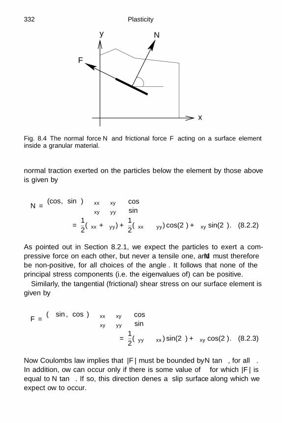
332 Plasticity
F
x
y N
θ
Fig. 8.4 The normal force N and frictional force F acting on a surface elementinside a granular material.
normal traction exerted on the particles below the element by those aboveis given by
N =(cos θ, sin θ)
(τxx τxy
τxy τyy
)(cos θ
sin θ
)=
12(τxx + τyy) +
12(τxx − τyy) cos(2θ) + τxy sin(2θ). (8.2.2)
As pointed out in Section 8.2.1, we expect the particles to exert a com-pressive force on each other, but never a tensile one, and N must thereforebe non-positive, for all choices of the angle θ. It follows that none of theprincipal stress components (i.e. the eigenvalues of τ) can be positive.
Similarly, the tangential (frictional) shear stress on our surface element isgiven by
F =(− sin θ, cos θ)
(τxx τxy
τxy τyy
)(cos θ
sin θ
)=
12(τyy − τxx) sin(2θ) + τxy cos(2θ). (8.2.3)
Now Coulomb’s law implies that |F | must be bounded by N tanφ, for all θ.In addition, flow can occur only if there is some value of θ for which |F | isequal to N tan φ. If so, this direction defines a slip surface along which weexpect flow to occur.

8.2 Models for granular material 333
N
F
φ
√14(τxx − τyy)2 + τ 2
xy
−τxx + τyy
2
Fig. 8.5 The Mohr circle in the (N,F )-plane, and the lines where |F | = |N | tan φ.
From (8.2.2) and (8.2.3), we see that, as θ varies, the tractions lie on theso-called Mohr circle in the (N, F ) plane, given by
F 2 +(
N − 12(τxx + τyy)
)2
=(τxx − τyy)2
4+ τ 2
xy, (8.2.4)
where different points on the circle correspond to different choices of theangle θ. Since we require N to be non-positive for all θ, the Mohr circle mustlie in the half-plane N 0, as shown in Figure 8.5. Coulomb’s law then tellsus that |F | |N | tan φ for all θ, and the Mohr circle must therefore liein the sector N tan φ F −N tan φ. Finally, if the material is flowing,then there must be one value of θ such that |F | = |N | tan φ, and the Mohrcircle must therefore be tangent to the lines |F | = |N | tanφ, as shown inFigure 8.5.
Elementary trigonometry now tells us that the stress components in agranular material must satisfy
2(τxxτyy − τ 2
xy
)1/2 −(τxx + τyy) cos φ. (8.2.5)
When the material is flowing and equality holds, (8.2.5) is called the Coulombyield criterion. Notice that (8.2.5) is a relation between the two stress invari-ants Tr (τ) and det (τ). This is reassuring, since it implies that the conditionfor the material to yield is independent of our choice of coordinate system.
We can only make significant analytical progress if we assume that theflow is slow enough for the inertia of the particles to be negligible in

334 Plasticity
comparison with the frictional forces between them and, perhaps, gravity.This assumption is often valid in practice and allows us to neglect the ac-celeration term in Cauchy’s momentum equation, which thus reduces to
∂τxx
∂x+
∂τxy
∂y= 0,
∂τxy
∂x+
∂τyy
∂y+ ρg = 0. (8.2.6)
Given our restriction to two dimensions, we see that (8.2.6) and the yieldcriterion (8.2.5) give us three equations in the three stress components τxx,τxy and τyy . It is therefore possible, in principle, to solve for the stresstensor in a flowing granular material in two dimensions without specifyingany particular constitutive relation. This is in stark contrast with all theoriesof elasticity that we have encountered thus far.
The easiest case to analyse occurs when gravity is negligible so we can use(8.2.6) to introduce an Airy stress function A. Then, when the material isflowing, equality in (8.2.5) implies a nonlinear partial differential equationfor A, namely
∂2A
∂x2∂2A
∂y2 −(
∂2A
∂x∂y
)2
=cos2 φ
4(∇2A
)2. (8.2.7)
When φ = π/2, this reduces to the Monge–Ampere equation encounteredpreviously in Chapter 4. When φ ∈ (0, π/2), (8.2.7) is, unexpectedly, ahyperbolic partial differential equation.
Even with the body force included, the system (8.2.5), (8.2.6) is likewisehyperbolic, as shown in Exercise 8.3. This means that the stress field in theflowing material is confined to certain regions of influence bounded by therelevant characteristics of (8.2.7). Outside these regions, the inequality in(8.2.5) is strict, so the granular material does not flow but behaves like anelastic solid and hence satisfies elliptic equations. By combining these tworegimes, we obtain a perfectly plastic theory, as described in Section 8.1, inwhich the yield stress is never exceeded. The key to solving such models is tolocate the free boundary that separates the flowing and non-flowing regions.The switch in behaviour from hyperbolic to elliptic makes these problemsvery difficult in general, but there are a handful of symmetric situationswhere we can find an explicit solution.
8.2.3 Example: a tunnel in granular rock
One such configuration is the problem of a circular tunnel of radius a boredthrough granular rock, subject to a uniform isotropic pressure p∞ at infinityand a positive pressure P at r = a to simulate the tunnel bracing.† To model†
Had we included a depth-dependent hydrostatic pressure at infinity, as in Section 2.6.9, ana-lytical progress would have been considerably more difficult.

8.2 Models for granular material 335
this situation, we seek an axisymmetric solution in which the displacementis purely radial, with u = ur(r)er , and the only nonzero in-plane stresscomponents are τrr(r) and τθθ(r). As in Section 2.6.5, the use of an Airystress function is somewhat awkward in this multiply connected domain, andit is more convenient to work directly with the plane polar Navier equation
dτrr
dr+
τrr − τθθ
r= 0. (8.2.8)
The boundary conditions on the tunnel wall and in the far field read
τrr = −P on r = a, (8.2.9a)
τrr → −p∞, τθθ → −p∞ as r → ∞. (8.2.9b)
By rotating the axes, we can write (8.2.5) in the form
2 (τrrτθθ)1/2 − cos φ (τrr + τθθ) . (8.2.10)
Hence yield occurs when
kτrr = τθθ, (8.2.11)
where the so-called triaxial stress factor k satisfies
2k1/2 = (1 + k) cos φ. (8.2.12)
While the rock remains elastic, we can use the usual constitutive relations(1.11.5):
τrr = (λ + 2µ)dur
dr+ λ
ur
r, τθθ = λ
dur
dr+ (λ + 2µ)
ur
r. (8.2.13)
Then it is straightforward to solve (8.2.8) and (8.2.9) to find
ur = − p∞r
2(λ + µ)+
(P − p∞)a2
2µr, (8.2.14)
and the stress components are then given by
τrr = −p∞ + (p∞ − P )a2
r2 , τθθ = −p∞ − (p∞ − P )a2
r2 . (8.2.15)
Notice the analogy between (8.2.14) and the gun barrel solution (2.6.41),with the outer radius b tending to infinity and a superimposed isotropicpressure.
At the tunnel wall r = a, we have
τθθ
τrr=
2p∞P
− 1, (8.2.16)

336 Plasticity
0.2 0.4 0.6 0.8 1.0 1.2 1.4
5
10
15
20
φ
k
Fig. 8.6 The triaxial stress factor k defined by (8.2.18) versus angle of friction φ.
so, as P is lowered below p∞, yield will first occur when
P =2p∞1 + k
. (8.2.17)
Since, again at r = a, we have τθθ − τrr = 2(P −p∞), we expect |τrr | = −τrr
to be less than |τθθ | = −τθθ . This means that we must choose the root of(8.2.12) that exceeds unity, namely
k =1 + sin φ
1 − sin φ. (8.2.18)
As shown in Figure 8.6, k is an increasing function of φ, with k → ∞ asφ → π/2. Hence (8.2.17) implies that, as the angle of friction increases, asmaller internal pressurisation is needed to prevent yield: the closer φ isto π/2, the stronger will be the tunnel.
Once P drops below the value given by (8.2.17), we can seek a compositeelastic-plastic solution in which there is a free boundary r = s separatingan elastic region in r > s from a perfectly plastic region in a < r < s, withkτrr = τθθ on r = s. Hence, to obtain the elastic solution in r > s, we simplyreplace P by 2p∞/(1 + k) and a by s in (8.2.15) to give
τrr = −p∞ + p∞
(k − 1k + 1
)s2
r2 , τθθ = −p∞ − p∞
(k − 1k + 1
)s2
r2 . (8.2.19)
Meanwhile, in the plastic region r < s, the quasistatic balance (8.2.8) isnow supplemented by the yield condition (8.2.11). The resulting equation
dτrr
dr+
1 − k
rτrr = 0, (8.2.20)

8.3 Dislocation theory 337
along with the boundary condition (8.2.9a), gives
τrr = −P(r
a
)k−1. (8.2.21)
Finally, equating (8.2.19) and (8.2.21) at r = s gives the radius of the plasticregion as
s = a
(2p∞
(k + 1)P
)1/(k−1)
. (8.2.22)
The above calculation leaves open the role played by the out-of-planestress tensor τzz , and we will return to this issue shortly. Moreover, we havegiven no way of predicting the flow velocity itself in the yielded region. Wehave suggested that the flow might occur along slip surfaces, but, even withthat assumption, some additional information is needed to determine themagnitude of the velocity. There are many empirical theories for this, andwe shall not attempt to review them here. Of course, matters would beeven worse if the velocity were large enough to invalidate our neglecting theacceleration term in (8.2.6), in which case the stress and velocity componentswould satisfy a fundamentally coupled problem.
It is remarkable that the theory that we have presented can successfullybe applied to situations ranging from the flow of powders to the design ofindustrial-scale coal hoppers. Moreover, it is relatively simple to generaliseour elastic-plastic theory to granular materials in which cohesive forces act,perhaps as a result of moisture. Then a tensile stress can be sustained, andall we have to do is to replace N by (N + c) in (8.2.4), where c is a positivecohesive force. However, it is far more difficult to extend the analysis tothree dimensions. To do this, the first task is to generalise the yield criterion(8.2.5), as shown in Exercise 8.2. However, this condition, along with themomentum equations (8.2.6), gives us only four scalar equations in the sixstress components, so the three-dimensional problem is inevitably under-determined without the imposition of a constitutive relation, and we willdiscuss this situation further in Section 8.4.3.
We now turn our attention to metal plasticity, for which the microscopicmathematical theory is somewhat better developed.
8.3 Dislocation theory
Metals can exhibit microstructure at several scales, depending how theyhave been solidified and whether there are alloying components. From thepoint of view of plasticity, the basic microstructure is that of a periodiclattice of atoms, and the crucial scale is one small enough for the atom
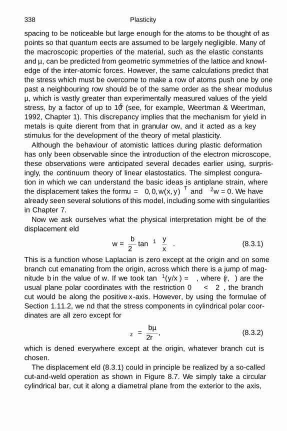
338 Plasticity
spacing to be noticeable but large enough for the atoms to be thought of aspoints so that quantum effects are assumed to be largely negligible. Many ofthe macroscopic properties of the material, such as the elastic constants λ
and µ, can be predicted from geometric symmetries of the lattice and knowl-edge of the inter-atomic forces. However, the same calculations predict thatthe stress which must be overcome to make a row of atoms push one by onepast a neighbouring row should be of the same order as the shear modulusµ, which is vastly greater than experimentally measured values of the yieldstress, by a factor of up to 105 (see, for example, Weertman & Weertman,1992, Chapter 1). This discrepancy implies that the mechanism for yield inmetals is quite different from that in granular flow, and it acted as a keystimulus for the development of the theory of metal plasticity.
Although the behaviour of atomistic lattices during plastic deformationhas only been observable since the introduction of the electron microscope,these observations were anticipated several decades earlier using, surpris-ingly, the continuum theory of linear elastostatics. The simplest configura-tion in which we can understand the basic ideas is antiplane strain, wherethe displacement takes the form u =
(0, 0, w(x, y)
)T and ∇2w = 0. We havealready seen several solutions of this model, including some with singularitiesin Chapter 7.
Now we ask ourselves what the physical interpretation might be of thedisplacement field
w =b
2πtan−1
(y
x
). (8.3.1)
This is a function whose Laplacian is zero except at the origin and on somebranch cut emanating from the origin, across which there is a jump of mag-nitude b in the value of w. If we took tan−1(y/x) = θ, where (r, θ) are theusual plane polar coordinates with the restriction 0 θ < 2π, the branchcut would be along the positive x-axis. However, by using the formulae ofSection 1.11.2, we find that the stress components in cylindrical polar coor-dinates are all zero except for
τθz =bµ
2πr, (8.3.2)
which is defined everywhere except at the origin, whatever branch cut ischosen.
The displacement field (8.3.1) could in principle be realized by a so-calledcut-and-weld operation as shown in Figure 8.7. We simply take a circularcylindrical bar, cut it along a diametral plane from the exterior to the axis,

8.3 Dislocation theory 339
yx
z
Fig. 8.7 An antiplane cut-and-weld operation leading to the displacement field(8.3.1).
displace one side of the cut by a distance b relative to the other side, andfinally weld the two cut faces together again. Clearly there will be a regionof very large strain close to the axis, in accordance with (8.3.2). We willthus have created a bar that is in a state of self-stress, so that it is inequilibrium under the action of no external forces, yet there is a nonzerostress distribution in the interior.
We can also interpret (8.3.1) in terms of incompatibility. We recall fromSection 2.7 that the assumption of a single-valued displacement field givesrise to compatibility relations between the strain components. Since (8.3.1)is not single-valued, we would expect these relations to be violated. Indeed,in Exercise 8.4 we show that w satisfies
∂2w
∂y∂x− ∂2w
∂x∂y= bδ(x)δ(y), (8.3.3)
where δ denotes the Dirac delta-function defined in Section 2.9.1. We caninterpret (8.3.3) as a “failure of single-valuedness” or a line of incompatibilityalong the z-axis.
It is also instructive to introduce an antiplane stress function φ, as inSection 2.4, defined to be the harmonic conjugate of w so that w and φ
satisfy the Cauchy–Riemann equations
∂w
∂x=
∂φ
∂y,
∂w
∂y= −∂φ
∂x. (8.3.4)

340 Plasticity
(a) (b)
x
y y
x
Fig. 8.8 The displacement field in an edge dislocation: (a) pristine material; (b) afterthe cut-and-weld operation.
Now, the harmonic conjugate of (8.3.1) is φ = −(b/2π) log r, which, as weknow from Section 2.9.1, satisfies
∇2φ = −bδ(x)δ(y), (8.3.5)
and we can easily verify that (8.3.5) is consistent with (8.3.3). The singularityin (8.3.1) at x = y = 0 is thus analogous to the singularity at the core of a linevortex in inviscid fluid dynamics, where a finite circulation is concentratedon a line in an otherwise irrotational flow.
Similar behaviour occurs if we displace one cut face radially relativeto the other before welding them back together, as shown in Figure 8.8.This configuration can be described using a plain strain displacement fieldu =
(u(x, y), v(x, y), 0
)T, in which u is discontinuous across the positivex-axis. We can find such a displacement by using the Papkovich–Neuberrepresentation used in Section 2.8.6, namely
2µu = 2(1 − ν)
ψ1
ψ2
0
− grad(
φ +xψ1 + yψ2
2
), (8.3.6)
where ψ1, ψ2 and φ are all harmonic functions of x and y. Now the requireddiscontinuity in u may be obtained by choosing φ = 0, ψ1 proportional to θ
and ψ2 equal to a constant.As shown in Exercise 8.5, this approach leads us to the displacement field(
u
v
)=
b
2π
(θ
0
)+
b sin θ
2π(3 − 4ν)
(cos θ
sin θ
)(8.3.7)
which is depicted in Figure 8.8. The associated stress field is given in

8.3 Dislocation theory 341
(a) (b)
Fig. 8.9 An edge dislocation in a square crystal lattice: (a) pristine crystal; (b) in-sertion of an extra row of atoms.
cylindrical polar coordinates byτrr τrθ τrz
τrθ τθθ τθz
τrz τθz τzz
=
2µb
π(3 − 4ν)r
−ν sin(θ) (1 − ν) cos(θ) 0(1 − ν) cos(θ) −(1 − ν) sin(θ) 0
0 0 −ν sin(θ)
, (8.3.8)
so we again have a state of self-stress which is infinite on the line r = 0.Exercise 8.6 shows that (8.3.8) corresponds to an Airy stress function
A =−µb
π(3 − 4ν)(1 − 2ν)rθ cos θ + 2(1 − ν)r log r sin θ , (8.3.9)
which satisfies the equation
∇4A =(
4µb
(3 − 4ν)
)δ(x)δ′(y), (8.3.10)
which is effectively (2.9.48). Now we recall from Section 2.8.2 that the exis-tence of A ensures that the plane strain Navier equations are satisfied, whilethe biharmonic equation for A was obtained by assuming compatibility be-tween the strain components. Hence, as in (8.3.3), we can interpret (8.3.10)as describing a line of incompatibility along the z-axis.
A key insight into the physical mechanism for plastic flow in metals comeswhen we imagine executing the cut-and-weld operation shown in Figure 8.8at an atomic scale. For example, on the square lattice shown in Figure 8.9(a),we can achieve this by inserting an extra column of atoms, as depicted inFigure 8.9(b). This figure is effectively the same as Figure 8.8(b) after the“ledge” below the positive x-axis has been removed. Far from the crystalmisfit, it simply seems that the atoms below the positive x-axis have beendisplaced one atom spacing to the right, as in the displacement field (8.3.7).We are thus led to conjecture that, with b equal to a single atomic spacing,

342 Plasticity
(a) (b) (c) (d)
Fig. 8.10 A moving edge dislocation: (a) initial configuration; (b) and (c) the dis-location moves to the left as the atoms realign themselves, eventually (d) leadingto a net displacement of the upper block of atoms relative to the lower.
an atomistic calculation of the displacement based on Figure 8.9(b) wouldtend to (8.3.7) on a scale large compared to b.†
The region near the z-axis within a few atomic spacings of the crystalmisfit is called the core of an edge dislocation, the corresponding regionin the antiplane configuration analogous to Figure 8.7 being the core of ascrew dislocation. The dislocation itself, in either case, is the z-axis and thedisplacement jump as we move around any curve enclosing the dislocationis called the Burgers vector. In our examples, the Burgers vector is (0, 0, b)T
for the screw dislocation and (b, 0, 0)T for the edge dislocation. However,it is quite easy to take linear combinations of these to generate a mixeddislocation along the z-axis which is part edge and part screw. In addition,we can envisage dislocations on a macroscopic scale which lie on curvedrather than straight lines, by identifying the z-axis with the tangent to thedislocation at any point. In practice, the symmetries of the crystal latticeusually force any dislocations to lie in certain planes, known as slip planes,to which the Burgers vector is tangent (Hirth & Lothe, 1991, p. 271). Incontrast with granular flow, where there is just one direction of slip at anypoint, there may be many slip planes, depending on the symmetries of thecrystal structure. These are set in the metal, whereas the slip planes in agranular material depend on the stress state.
Anything other than an absolutely perfect crystal must contain manydislocations like that shown in Figure 8.9(b). Now the key observation isthat just a small realignment of the atoms near the core is needed for sucha dislocation to move irreversibly through the lattice. This is illustratedschematically in Figure 8.10, where a dislocation moves to the left, therebymoving the lower block of atoms bodily with respect to the upper block.
†Of course we are not really justified in using the atomic scale b in a macroscopic model like(8.3.1). Indeed the key challenge in the theoretical modelling of dislocations is to make theconnection between atomic and macroscopic scales.

8.3 Dislocation theory 343
This can be achieved without forcing large numbers of atoms to slide overeach other, and this explains the huge discrepancy noted above betweenpredictions of the yield stress based on inter-atomic forces and experimen-tally measured values. We also note for future reference that the configu-rational changes illustrated in Figure 8.10 take place with no appreciablechange in volume of the crystal.
All these observations led theoreticians in the 1930s and earlier to sug-gest that macroscopic metal plasticity could be explained by the motionof dislocations, and it was a great day when, two decades later, electronmicrographs of metal crystals that had undergone plastic deformation wereable to confirm the theory. They revealed countless (up to 1012 cm−2) blackcurves in regions which would have been invisible had the crystal been per-fect. Each of these curves represented a dislocation bounding a plane regionof slip in the crystal and, the more the metal had been deformed plastically,the more black lines were observed.
Since any realistic sample contains so many dislocations, it is impracticalto track each one individually. Instead, any macroscopic theory must usea density, which is in fact a tensor,† that characterises the direction andBurgers vector averaged over a large number of dislocations. Moreover, itwould need a rule for how dislocations move, analogous to that used toobtain a model for collective motion of vortices in an inviscid fluid or ofsuperconducting vortices in a type-II superconductor. Unfortunately, it hasproved much harder to carry this out in practice for dislocations, and adefinitive macroscopic model does not yet exist.
Rather than delving further into this fascinating open problem, we willsimply use microscopic thought-experiments like Figure 8.10 to suggest thefollowing guidelines that will be employed below to obtain a closed macro-scopic model for metal plasticity.
(i) Dislocations may move under the action of an applied shear stress, butare generally impervious to any isotropic pressure.
(ii) Collective motion of many dislocations can only occur when a suffi-ciently high shear stress exists at every point. The critical yield stressis a constant for any given metal.
(iii) Plastic flow, which results from collective dislocation motion, is essen-tially incompressible.
These conjectures can be tested experimentally or by performing atomisticcomputations on a discrete lattice.†
furthermore, such a density tensor would have to vanish in regions in which the incompatibilitytensor (2.9.46) vanishes
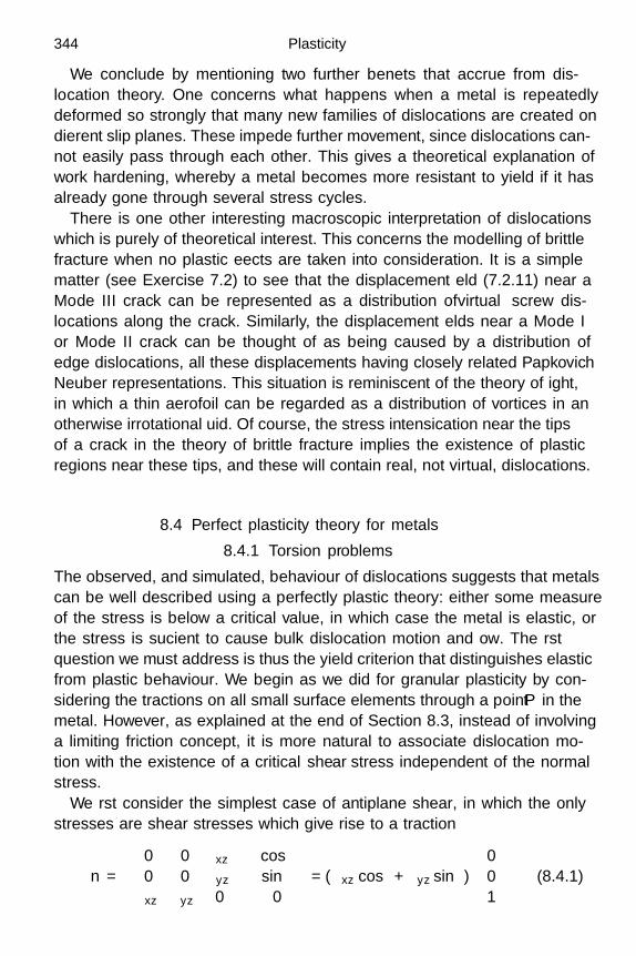
344 Plasticity
We conclude by mentioning two further benefits that accrue from dis-location theory. One concerns what happens when a metal is repeatedlydeformed so strongly that many new families of dislocations are created ondifferent slip planes. These impede further movement, since dislocations can-not easily pass through each other. This gives a theoretical explanation ofwork hardening, whereby a metal becomes more resistant to yield if it hasalready gone through several stress cycles.
There is one other interesting macroscopic interpretation of dislocationswhich is purely of theoretical interest. This concerns the modelling of brittlefracture when no plastic effects are taken into consideration. It is a simplematter (see Exercise 7.2) to see that the displacement field (7.2.11) near aMode III crack can be represented as a distribution of virtual screw dis-locations along the crack. Similarly, the displacement fields near a Mode Ior Mode II crack can be thought of as being caused by a distribution ofedge dislocations, all these displacements having closely related Papkovich–Neuber representations. This situation is reminiscent of the theory of flight,in which a thin aerofoil can be regarded as a distribution of vortices in anotherwise irrotational fluid. Of course, the stress intensification near the tipsof a crack in the theory of brittle fracture implies the existence of plasticregions near these tips, and these will contain real, not virtual, dislocations.
8.4 Perfect plasticity theory for metals
8.4.1 Torsion problems
The observed, and simulated, behaviour of dislocations suggests that metalscan be well described using a perfectly plastic theory: either some measureof the stress is below a critical value, in which case the metal is elastic, orthe stress is sufficient to cause bulk dislocation motion and flow. The firstquestion we must address is thus the yield criterion that distinguishes elasticfrom plastic behaviour. We begin as we did for granular plasticity by con-sidering the tractions on all small surface elements through a point P in themetal. However, as explained at the end of Section 8.3, instead of involvinga limiting friction concept, it is more natural to associate dislocation mo-tion with the existence of a critical shear stress independent of the normalstress.
We first consider the simplest case of antiplane shear, in which the onlystresses are shear stresses which give rise to a traction
τn =
0 0 τxz
0 0 τyz
τxz τyz 0
cos θ
sin θ
0
= (τxz cos θ + τyz sin θ)
001
(8.4.1)
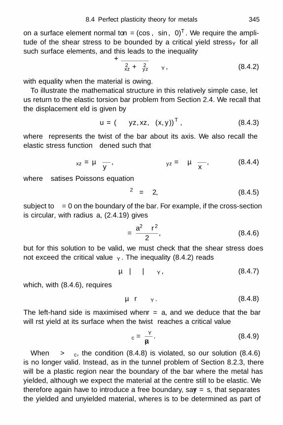
8.4 Perfect plasticity theory for metals 345
on a surface element normal to n = (cos θ, sin θ, 0)T. We require the ampli-tude of the shear stress to be bounded by a critical yield stress τY for allsuch surface elements, and this leads to the inequality√
τ 2xz + τ 2
yz τY , (8.4.2)
with equality when the material is flowing.To illustrate the mathematical structure in this relatively simple case, let
us return to the elastic torsion bar problem from Section 2.4. We recall thatthe displacement field is given by
u = Ω (−yz, xz, ψ(x, y))T , (8.4.3)
where Ω represents the twist of the bar about its axis. We also recall theelastic stress function φ defined such that
τxz = µΩ∂φ
∂y, τyz = −µΩ
∂φ
∂x, (8.4.4)
where φ satisfies Poisson’s equation
∇2φ = −2, (8.4.5)
subject to φ = 0 on the boundary of the bar. For example, if the cross-sectionis circular, with radius a, (2.4.19) gives
φ =a2 − r2
2, (8.4.6)
but for this solution to be valid, we must check that the shear stress doesnot exceed the critical value τY. The inequality (8.4.2) reads
µΩ |∇φ| τY , (8.4.7)
which, with (8.4.6), requires
µΩr τY . (8.4.8)
The left-hand side is maximised when r = a, and we deduce that the barwill first yield at its surface when the twist Ω reaches a critical value
Ωc =τY
µa. (8.4.9)
When Ω > Ωc, the condition (8.4.8) is violated, so our solution (8.4.6)is no longer valid. Instead, as in the tunnel problem of Section 8.2.3, therewill be a plastic region near the boundary of the bar where the metal hasyielded, although we expect the material at the centre still to be elastic. Wetherefore again have to introduce a free boundary, say r = s, that separatesthe yielded and unyielded material, where s is to be determined as part of
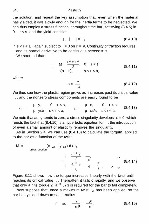
346 Plasticity
the solution, and repeat the key assumption that, even when the materialhas yielded, it flows slowly enough for the inertia terms to be neglected. Wecan thus employ a stress function φ throughout the bar, satisfying (8.4.5) in0 r < s and the yield condition
µΩ |∇φ| = τY (8.4.10)
in s < r < a, again subject to φ = 0 on r = a. Continuity of traction requiresφ and its normal derivative to be continuous across r = s.
We soon find that
φ =
as − s2 + r2
2, 0 r < s,
s(a − r), s < r < a,(8.4.11)
where
s =τY
Ωµ. (8.4.12)
We thus see how the plastic region grows as Ω increases past its critical valueΩc, and the nonzero stress components are easily found to be
τxz =
−µΩy, 0 r < s,
−µΩys/r, s < r < a,τyz =
µΩx, 0 r < s,
µΩxs/r, s < r < a.(8.4.13)
We note that as τY tends to zero, a stress singularity develops at r = 0, whichreflects the fact that (8.4.10) is a hyperbolic equation for φ; the introductionof even a small amount of elasticity removes the singularity.
As in Section 2.4, we can use (8.4.13) to calculate the torque M appliedto the bar as a function of the twist
M =∫∫
cross-section(xτyz − yτxz) dxdy
=
(
πa3τY
2
)ΩΩc
, Ω Ωc,(πa3τY
6
)(4 − Ω3
c
Ω3
), Ω > Ωc.
(8.4.14)
Figure 8.11 shows how the torque increases linearly with the twist until Ωreaches its critical value Ωc. Thereafter, it tails off rapidly, and we observethat only a finite torque 2πa3τY/3 is required for the bar to fail completely.
Now suppose that, once a maximum twist ΩM has been applied, so thebar has yielded down to some radius
r = sM =τY
ΩMµ=
Ωca
ΩM, (8.4.15)

8.4 Perfect plasticity theory for metals 347
0 1 2 3 4
0.2
0.4
0.6
0.8
1.0
1.2
1.4
Ω/Ωc
2M/πa3τY
Fig. 8.11 The normalised torque M versus twist Ω applied to an elastic-plasticcylindrical bar.
the applied torque is then removed sufficiently slowly that we can still usea quasistatic model. We would expect the bar to recover and twist backtowards its starting configuration. We denote this subsequent displacementby u; in other words, u is the displacement relative to the state just beforewe released the torque. Consistent with our assumption of perfect plasticityis the further assumption that, as soon as the torque is decreased, all theonce-yielded material instantly returns to being elastic. However, it will nowstart with the nonzero stress (8.4.13) when u is zero.
Let us suppose that u has the same structure (8.4.3) as the original dis-placement, that is
u = Ω (−yz, xz, 0)T , (8.4.16)
since we recall from Section 8.2 that ψ ≡ 0 for a circular bar. The net twistof the bar is given by ΩM +Ω, so we expect Ω to start at zero when Ω = ΩM
and then fall to negative values as the bar is unloaded. The total stressconsists of the elastic stress corresponding to (8.4.16) added to the initialstress (8.4.13) reached at the end of the plastic phase, that is
(τxz
τyz
)= µ
(−y
x
)×
(Ω + ΩM
), 0 r < sM ,(
Ω + ΩMsM/r), sM < r < a.
(8.4.17)
A calculation analogous to (8.4.14) leads to the following formula for theapplied torque during the recovery phase:
2M
πµa4 = Ω +Ωc
3
(4 − Ω3
c
Ω3M
). (8.4.18)
The final resultant twist Ω0 when the torque has been completely released

348 Plasticity
0.0 0.5 1.0 1.5 2.0 2.5 3.0
0.2
0.4
0.6
0.8
1.0
1.2
Ω/Ωc
2M/πa3τY plastic
elastic
ΩM/Ωc
recovery
Ω0/Ωc
Fig. 8.12 The normalised torque M versus twist Ω applied to an elastic-plasticcylindrical bar, showing the recovery phase when the torque is released.
is thus found by setting M = 0 in (8.4.18) and recalling that Ω = ΩM + Ω:
Ω0
Ωc=
ΩM
Ωc+
Ω3c
3Ω3M
− 43. (8.4.19)
When ΩM = Ωc (so the bar has never yielded), we see that Ω0 = 0, sothe bar returns to its original configuration upon unloading. However, asthe maximum twist ΩM is increased, a decreasing fraction of it is recoveredwhen the torque is released, as illustrated in Figure 8.12. The bar behaveselastically until Ω = Ωc and then starts to yield. When M returns to zero,a nonzero twist remains, and this qualitative behaviour is typical of elastic-plastic systems.
The final crucial observation is that, even when the bar has recoveredand there is no net torque on it, the internal stress components (8.4.17)are nonzero, and the bar is said to contain residual stress. This is bound tohappen because the recovery phase starts with an initial stress field (8.4.13)that does not satisfy the compatibility conditions. This means that thereis no elastic deformation that the material can adopt that will completelyrelieve the stress.
Without the assumption of radial symmetry, the problem must in generalbe solved numerically, but it still possesses a very helpful mathematicalstructure, in which the general scenario is sketched in Figure 8.13. Thereis a plastic region near the boundary in which we have to solve the eikonalequation (8.4.10). This equation is hyperbolic and, given φ = 0 on thesurface of the bar, can in principle be solved for φ throughout the plasticregion. In the elastic region, φ still satisfies Poisson’s equation, subject to

8.4 Perfect plasticity theory for metals 349
y
x
∇2φ = −2
Elastic
Plastic
|∇φ|2 =τ 2Y
µ2Ω2
φ = 0
[φ]
=
[∂φ
∂n
]= 0
Fig. 8.13 The free-boundary problem for an elastic-perfectly plastic torsion bar.
two boundary conditions, namely that both φ and its normal derivative arecontinuous. In principle, this problem determines both φ and the positionof the free boundary between the elastic and plastic regions.
This switch in behaviour across the free boundary is reminiscent of thecomplementarity conditions encountered when modelling contact problemsin Chapter 7. Indeed, the free-boundary problem depicted in Figure 8.13may be cast as a variational inequality and hence proved to be well posed,despite the nonlinearity and the change of type from hyperbolic to elliptic.Moreover, in most practical cases it can be proved to be equivalent to theproblem of minimising
∫∫D
(|∇φ|2 − 4φ
)dxdy
over all sufficiently smooth functions that vanish on the outer boundary andare such that |∇φ| τY/µΩ.
We also note that, as in our models for granular materials, although theyield condition enables us to determine the stress, it tells us nothing aboutthe displacement in the bar once it has yielded. We will return to this pointin Section 8.10.

350 Plasticity
8.4.2 Plane strain
The next simplest situation is that of plane strain, where we can follow theapproach of Section 8.2.2 to calculate the shear stress on a surface elementwith unit normal n = (cos θ, sin θ, 0)T. Indeed, we can read off the maximumtangential traction F by inspecting the Mohr circle in Figure 8.5, and hencededuce the inequality √
14 (τxx − τyy)2 + τ 2
xy τY , (8.4.20)
with equality when the material has yielded. As in Section 8.4.1, our taskis very much easier if we assume that any plastic flow occurs sufficientlyslowly for the momentum terms in the Navier equation to be negligible.Hence, we can conveniently use an Airy stress function A throughout thematerial.
Where the material has not yielded (so the inequality in (8.4.20) is strict),we obtain
∇4A = 0, (8.4.21)
as in Section 2.6.2. However, when yield occurs, we have equality in (8.4.20),and A satisfies
(∇2A
)2 + 4
(∂2A
∂x∂y
)2
− ∂2A
∂x2∂2A
∂y2
= 4τ 2
Y . (8.4.22)
As always the key aspect of the problem is to locate the boundary where theswitch from (8.4.21) to (8.4.22) occurs. Here, a traction balance shows thatA and its first and second partial derivatives must all be continuous acrosssuch a boundary.
The nonlinear partial differential equation (8.4.22) satisfied by A when thematerial has yielded is another generalisation of the Monge–Ampere equa-tion, and closely resembles the equation (8.2.7) for granular flow in planestrain. It is not immediately classifiable using the standard theory of second-order partial differential equations, but the method of Exercise 4.12 showsthat it is hyperbolic, with two families of real characteristicssatisfying
dy
dx= 2
(∂2A
∂x∂y± τY
)/(∂2A
∂x2 − ∂2A
∂y2
). (8.4.23)
These correspond to the directions in which the shear stress is maximal (seeExercise 8.8), and hence the characteristics of (8.4.22) are the slip surfaces,along which we might expect the material to flow.
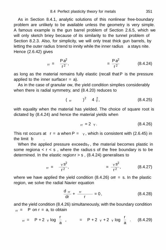
8.4 Perfect plasticity theory for metals 351
As in Section 8.4.1, analytic solutions of this nonlinear free-boundaryproblem are unlikely to be available unless the geometry is very simple.A famous example is the gun barrel problem of Section 2.6.5, which wewill only sketch briefly because of its similarity to the tunnel problem ofSection 8.2.3. Also, for simplicity, we will only treat thick gun barrels, byletting the outer radius b tend to infinity while the inner radius a stays finite.Hence (2.6.42) gives
τrr = −Pa2
r2 , τθθ =Pa2
r2 (8.4.24)
as long as the material remains fully elastic (recall that P is the pressureapplied to the inner surface r = a).
As in the case of granular flow, the yield condition simplifies considerablywhen there is radial symmetry, and (8.4.20) reduces to
(τrr − τθθ)2 4τ 2
Y , (8.4.25)
with equality when the material has yielded. The choice of square root isdictated by (8.4.24) and hence the material yields when
τθθ − τrr = 2τY . (8.4.26)
This first occurs at r = a when P = τY, which is consistent with (2.6.45) inthe limit b → ∞.
When the applied pressure exceeds τY, the material becomes plastic insome region a < r < s, where the radius s of the free boundary is to bedetermined. In the elastic region r > s, (8.4.24) generalises to
τrr = −τYs2
r2 , τθθ =τYs2
r2 , (8.4.27)
where we have applied the yield condition (8.4.26) on r = s. In the plasticregion, we solve the radial Navier equation
dτrr
dr+
τrr − τθθ
r= 0, (8.4.28)
and the yield condition (8.4.26) simultaneously, with the boundary conditionτrr = −P on r = a, to obtain
τrr = −P + 2τY log(r
a
), τθθ = −P + 2τY + 2τY log
(r
a
). (8.4.29)

352 Plasticity
1.5 2.0 2.5 3.0
2.0
1.5
1.0
0.5
0.0
0.5
r/a
(τθθ − τrr) /τY PM = 2τY
PM = τY
Fig. 8.14 Residual shear stress τθθ − τrr in a gun barrel versus radial dis-tance r for different values of the maximum internal pressurisation: PM/τY =1, 1.25, 1.5, 1.75, 2.
Hence, when we balance the normal traction τrr at r = s, we find that
s = a exp(
P
2τY− 1
2
). (8.4.30)
This shows how the plastic region grows rapidly as P increases through τY.We can now perform an unloading analysis similar to that in Section 8.4.1.
Suppose P increases to a value PM greater than τY, before decreasing to zero.Our assumption that the material instantaneously becomes elastic whenP < PM means that, as in (8.4.17), the free boundary remains stuck atits maximum value sM = a exp (PM/2τY − 1/2). The subsequent response ispurely elastic so that
τrr = −τYs2M
r2 +a2 (PM − P )
r2 , τθθ =τYs2
Mr2 − a2 (PM − P )
r2 (8.4.31)
in r > sM, while
τrr = −PM + 2τY log(r
a
)+
a2 (PM − P )r2 , (8.4.32a)
τθθ = −PM + 2τY + 2τY log(r
a
)− a2 (PM − P )
r2 (8.4.32b)
in a < r < sM.As in the torsion bar problem of Section 8.4.1, there remains a residual
stress field when the loading P has returned to zero. As shown in Figure 8.14,the residual shear stress τθθ − τrr increases in magnitude as PM is increasedpast τY. The boundary r = a ends up in a state of negative shear stresswhich, if PM > 2τY, will be large enough to cause the metal to yield againas it recovers!
8.4 Perfect plasticity theory for metals 353
We have still given no procedure to calculate the displacements in theplastic region. We also caution that the above calculation completely ignoresthe role of τzz , and we will address this issue next.
8.4.3 Three-dimensional yield conditions
As we will soon discover, generalising the yield condition to three dimensionsintroduces new complications not encountered in the antiplane and planestrain examples considered above. In general, and not just for metals, weexpect to impose an inequality of the form
f (τij) τY , (8.4.33)
where the yield function f is some appropriate measure of the stress. Nowwe ask ourselves what restrictions need to be imposed on the function f toensure that (8.4.33) is physically realistic.
If we assume that our metal is isotropic, then f must be invariant underrotation of the axes. It follows that f can be written as a function of thethree stress invariants (cf Section 5.3.2)
I1(τ) = Tr (τ), I2(τ) =12
Tr (τ)2 − Tr
(τ 2) , I3(τ) = det (τ), (8.4.34)
and we have therefore reduced f from six degrees of freedom (the elementsof the symmetric tensor τij) to three. Recall, for example, that the Coulombyield criterion (8.2.5) for granular material in two dimensions depends onlyon I1(τ) and I3(τ).
For metals, further simplification can be achieved by recalling the experi-mental evidence that they do not deform plastically under an isotopic stress,for which τij = −pδij , say; indeed it is intuitively reasonable that a pres-sure could not cause a dislocation like that sketched in Figure 8.9 to move.†
Hence we expect that our yield function f should not vary if τij is replacedby τij + cδij , where c is any scalar, that is
f (τij + cδij) ≡ f (τij) . (8.4.35)
We can understand the implications of this constraint on f if we regardit not as a function of the six independent variables τij but as a function ofthe variables
τ ′ij = τij −
13(τkk)δij and p = −1
3τkk. (8.4.36)
Since τ ′kk = 0, the τ ′
ij comprise only five independent variables and they
†Other materials, for example glass, can, however, flow under sufficient hydrostatic pressure.

354 Plasticity
define a symmetric trace-free tensor known as the deviatoric part of τij orthe stress deviator, while p may be identified with the net isotropic pressure.We can thus write
f (τij) ≡ f ′ (τ ′ij , p
), (8.4.37)
say, and, in terms of f ′, the constraint (8.4.35) is transformed to
f ′ (τ ′ij , p − c
)≡ f ′ (τ ′
ij , p). (8.4.38)
Since this holds for all c, we deduce that f ′ is independent of p and thereforejust a function of τ ′
ij .Now we can impose invariance under both rigid-body rotation and isotropic
pressure by writing
f ′ (τ ′ij
)= f ′′ (τ ′
1, τ′2, τ
′3), (8.4.39)
where τ ′k are the eigenvalues of τ ′
ij . It is easy to see that the principal axesof τ ′
ij and τij coincide, and that τ ′k are related to the principal stresses τk
(k = 1, 2, 3) by
τ ′k = τk + p, where p = −τ1 + τ2 + τ3
3. (8.4.40)
Since τ ′1 + τ ′
2 + τ ′3 = 0, there are only two independent degrees of freedom
remaining in the function f ′′. Henceforth we will simply write f(τ ′k) to mean
f ′′(τ ′k), hopefully without causing too much confusion.
One physically plausible possibility is again to define f as the maximumshear stress acting on all possible surface elements. As shown in Exercise 2.9(see also Exercise 8.2), this leads to
f(τ ′1, τ
′2, τ
′3)
=12
max|τ ′
1 − τ ′2|, |τ ′
2 − τ ′3|, |τ ′
3 − τ ′1|
, (8.4.41)
and the corresponding yield condition
max|τ ′
1 − τ ′2|, |τ ′
2 − τ ′3|, |τ ′
3 − τ ′1|
= 2τY . (8.4.42)
is called the Tresca condition. Notice that the function (8.4.41) is symmetricwith respect to permutation of its arguments, so that there are no preferreddirections.
In antiplane strain, with the stress tensor given in (8.4.1), the principaldeviatoric stresses are easily found to be
τ ′1 = −
√τ 2xz + τ 2
yz , τ ′2 =
√τ 2xz + τ 2
yz , τ ′3 = 0, (8.4.43)

8.4 Perfect plasticity theory for metals 355
4
4
2
−2
−4
−4 −20
24
0
2 0 −2 −4
1.0
0.5
−1.0
−1.0
−0.5
−0.5
0.5 1.0
τ ′3
τ ′1
τ ′1
τ ′2
τ ′2
(a) (b)
Fig. 8.15 (a) The Tresca yield surface (8.4.42) plotted in the space of principalstress deviators (τ ′
1 , τ′2 , τ
′3) (normalised with τY), showing the intersection with the
π-plane τ ′1 + τ ′
2 + τ ′3 = 0. (b) The projection in the (τ ′
1 , τ′2)-plane.
so that the Tresca condition reproduces (8.4.2). In plane strain, we find that
τ ′1 =
τxx + τyy − 2τzz
6−√
14 (τxx + τyy)
2 +(τ 2xy − τxxτyy
), (8.4.44a)
τ ′2 =
τxx + τyy − 2τzz
6+√
14 (τxx + τyy)
2 +(τ 2xy − τxxτyy
), (8.4.44b)
τ ′3 =
2τzz − τxx − τyy
3, (8.4.44c)
so the Tresca condition is consistent with (8.4.20) provided τ ′3 lies between τ ′
1and τ ′
2. This explains the role played by τzz in the examples in Section 8.4.1and Section 8.4.2, and Exercise 8.9 gives the basis for how τzz should beincorporated into these examples.
In three-dimensional problems, we can represent (8.4.42) as a surface,known as the yield surface, in (τ ′
1, τ′2, τ
′3)-space. As shown in Figure 8.15(a),
the Tresca yield surface is a cylinder whose axis is in the direction (1, 1, 1)T
and whose cross-section viewed along the axis in the π-plane τ ′1 +τ ′
2 +τ ′3 = 0
is a hexagon. By also using the constraint τ ′1 + τ ′
2 + τ ′3 = 0, we can project
this surface onto (for example) the (τ ′1, τ
′2)-plane as the polygon
max|τ ′
1 − τ ′2|, |2τ ′
2 + τ ′1|, |2τ ′
1 + τ ′2|
= 2τY , (8.4.45)
depicted in Figure 8.15(b).In antiplane strain, we have τ ′
3 = 0 and hence τ ′1+τ ′
2 = 0. This straight lineintersects the polygon shown in Figure 8.15(b) at the two points(τ ′
1, τ′2) = (±τY ,∓τY), so the yield surface degenerates to just two points

356 Plasticity
4
4
2
0
−2
−4
−4−2
24
0
2 0 −2 −4
1.0
0.5
−0.5
−1.0 −0.5 0.5 1.0
−1.0
τ ′3
τ ′1
τ ′1
τ ′2
τ ′2
(a) (b)
Fig. 8.16 (a) The von Mises yield surface plotted in the space of principal stressdeviators (τ ′
1 , τ′2 , τ
′3) (normalised with τY), showing the intersection with the π-plane
τ ′1 + τ ′
2 + τ ′3 = 0. (b) The projection in the (τ ′
1 , τ′2)-plane.
in antiplane strain. However, even in plane strain, the whole hexagon comesinto play in general (see Exercise 8.9), and the situation is even worse inthree dimensions. The presence of the corners in the yield surface is wor-rying, since it implies non-smooth dependence of the solution on the stresscomponents. It also makes the Tresca condition awkward to implement ingeneral, and this has led to the adoption of the von Mises yield function
f(τ ′1, τ
′2, τ
′3)
=
((τ ′
1 − τ ′2)
2 + (τ ′2 − τ ′
3)2 + (τ ′
3 − τ ′1)
2
6
)1/2
. (8.4.46)
By construction, this is a valid measure of the stress with all the requiredproperties of invariance although, unlike the Tresca yield function, it has noimmediate interpretation in terms of a maximal shear stress.
In (8.4.46), we have defined f such that τY is still the critical yield stressunder pure shear. However, under a uniaxial stress, with τ2 = τ3 = 0,the von Mises criterion predicts that yield will occur when τ1 =
√3τY, in
contrast with the value 2τY predicted by the Tresca condition.The yield surface corresponding to (8.4.46), shown in Figure 8.16(a), is
still a cylinder whose axis points in the direction (1, 1, 1)T. However, elemen-tary geometry implies that its cross-section is circular so, in contrast withFigure 8.15, the von Mises yield surface is smooth. Again we can use theconstraint τ ′
1 + τ ′2 + τ ′
3 to project the surface onto the (τ ′1, τ
′2)-plane, where

8.4 Perfect plasticity theory for metals 357
it takes the form of an ellipse, namely
τ ′12 + τ ′
1τ′2 + τ ′
22 =
(τ ′1 − τ ′
2)2
4+
3 (τ ′1 + τ ′
2)2
4= τY , (8.4.47)
as shown in Figure 8.16(b). In antiplane strain, the Tresca and von Misesyield criteria coincide, but in higher dimensions (8.4.46) is often easier toimplement, especially when we notice that it may be written in terms of thenon-principal stress components as(
f(τ ′))2
=12
Tr((τ ′)2) =
12τ ′ijτ
′ij . (8.4.48)
The assumed indifference of f to isotropic stress means that the yieldsurface corresponding to any valid choice of yield function must always bea cylinder pointing in the direction (1, 1, 1)T. The corresponding picture ingranular flow is quite different. First, we recall that none of the principalstresses in a granular material may be positive. Second, the yield criterionfor a granular material depends explicitly on the normal as well as the shearstress, so no advantage is gained by introducing the stress deviator. Exer-cise 8.2 shows that, provided the principal stresses are numbered in order,the Coulomb yield condition is equivalent to
τ1 − τ3 = (τ1 + τ3) sin φ when τ1 τ2 τ3 0. (8.4.49)
This represents a segment of a plane through the origin in (τ1, τ2, τ3)-space,and six other segments are obtained by switching the orders of the prin-cipal stress components. Hence, the analogue of the hexagonal cylinder ofFigure 8.15 is a six-sided pyramid, the faces of the pyramid correspondingto the six permutations of the indices in (8.4.49). Indeed, invariance withrespect to permutation of the principal stresses implies that the yield sur-face in any isotropic medium must share the six-fold symmetry evident inFigures 8.15 and 8.17.
We have seen above that, in both antiplane and plane strain, the yieldcriterion and the steady Navier equations form a closed system of equationsfor the stress components. However, the same is not true of genuinely three-dimensional problems, since we now have just one yield criterion and threeNavier equations for the six stress components. Moreover if the plastic flowis sufficiently strong for the material inertia to be comparable to the yieldstress, the resulting system is under-determined even in two dimensions. Asin granular flow, the problem must be closed by incorporating a flow rulethat determines how the material responds to stress once it has yielded.

358 Plasticity
0
0
0
−2
−4
−2
−4
−4
−2
τ3
τ1
τ2
Fig. 8.17 The Coulomb yield surface plotted in the space of principal stresses(τ1 , τ2 , τ3) (with φ = π/6).
8.5 Kinematics
This is the first time in this book that we have tried to write down a mathe-matical model for irreversible flow, as opposed to elastic strain. Such modelsare inevitably more readily stated in terms of the velocity of the medium,rather than the displacement. We therefore introduce the velocity vectorv(x, t) defined as
v =∂x
∂t
∣∣∣∣X
=∂u
∂t
∣∣∣∣X
, (8.5.1)
where the time derivative is taken with the Lagrangian coordinate X heldfixed. It is convenient to introduce a shorthand for this convective or materialderivative, namely
DDt
=∂
∂t
∣∣∣∣X
≡ ∂
∂t
∣∣∣∣x
+ (v · ∇) , (8.5.2)
the latter identity following from the chain rule.By applying the convective derivative to u, we obtain a kinematic rela-
tionship,
v =∂u
∂t+ (v · ∇)u, (8.5.3)
between the displacement and velocity. We can rearrange this to an explicit
8.5 Kinematics 359
equation for v, namely
v =(I − ∇uT)−1 ∂u
∂t, (8.5.4)
recalling that ∇u denotes the displacement gradient tensor with entries∂uj/∂xi. Hence we can linearise, approximating v as simply the Euleriantime derivative of u, provided the displacement gradients are small. Thisassumption is usually fine for small displacements of elastic materials, andleads to the theory of linear elasticity as we have seen. However, a character-istic of plastic behaviour is the ability to suffer large permanent displacementwithout breaking. To describe such situations as the bending of a paper clip,we would need to retain the nonlinear terms in (8.5.3) and distinguish care-fully between Lagrangian and Eulerian time derivatives, as in Chapter 5.
As shown in Exercise 8.10, conservation of mass in a material flowing withvelocity v and density ρ leads to the equation
Dρ
Dt+ ρ div v = 0. (8.5.5)
In an incompressible medium, the density of each material element is con-served, and the velocity must therefore satisfy div v = 0.
Next, to describe the deformation of a flowing material, we introducethe concept of rate-of-strain. We recall that the strain tensor describes thechange in length of a small line element in the material, compared with itsinitial length. Once a material is flowing, it starts to “forget” its initial reststate, so it no longer makes sense to use the initial length as a benchmark.Instead, it is more natural to examine the instantaneous variation in a lineelement over a small time increment. This is not a book about fluid me-chanics, so we will not spell out all the details here (but see Exercise 8.11).Suffice it to say that the rate of change of the length of a line elementδx = (δx1, δx2, δx3)
T takes the form
ddt
(|δx|2
)= 2δxTDδx, (8.5.6)
where the rate-of-strain tensor is defined by†
Dij =12
(∂vi
∂xj+
∂vj
∂xi
)or D =
12(∇v + ∇vT) . (8.5.7)
If the strains are small enough for us to neglect the nonlinear terms in(8.5.3), then Dij is simply the time derivative of the linear strain tensor eij .Otherwise, the relationship between strain and rate-of-strain is complicated,†Note that fluid mechanics textbooks often omit the factor of 1/2 in the definition of Dij
360 Plasticity
but it is of fundamental importance in describing large strains of viscoelasticmaterials, as we will see in Section 9.2.
8.6 Conservation of momentum
By applying the convective derivative to the velocity vector, we find thatthe acceleration of the medium is given by
Dv
Dt=
∂v
∂t+ (v · ∇) v, (8.6.1)
and we can therefore write Cauchy’s momentum equation in the form
ρ
∂v
∂t+ (v · ∇)v
= ∇ · τ + ρg. (8.6.2)
Along with the yield condition
f(τ) = τY , (8.6.3)
this gives us four scalar equations so far for the nine unknowns τij and vi.Now our task is to obtain a constitutive relation for the stress field associatedwith a given flow velocity v. Before doing so, we will first derive an equationrepresenting conservation of energy.
8.7 Conservation of energy
In Chapter 1, we showed that the net mechanical energy, i.e. the sum of thekinetic and strain energies, is conserved in a linear elastic solid. In Chapter 5,we found that the same is true in a nonlinear elastic material provided weuse a hyperelastic constitutive law. However, irreversible plastic flow involvesa loss of mechanical energy, which is dissipated as heat: by flexing a largepaper clip a few times, one can get it to warm up appreciably. We canquantify this heating by performing an energy balance on a material volumeV (t) that moves with the deforming medium. We now make the importantassumption that no elastic strain energy is stored once the material hasyielded (this assumption will be revisited in Section 8.9). The net energy inV (t) is therefore given by
U =∫∫∫
V (t)
12ρ|v|2 + ρcT
dx, (8.7.1)
where the terms in the integrand correspond respectively to the kinetic en-ergy and the thermal energy associated with the absolute temperature T .

8.7 Conservation of energy 361
We will assume that the parameter c, called the specific heat capacity (atconstant volume), is constant.
In accordance with the first law of thermodynamics, the energy inside V
will change because of (i) work done by stress on the boundary ∂V , (ii) workdone by the body force g on the interior of V and (iii) heat conductionthrough ∂V . Combining these effects together, we obtain
dU
dt=∫∫
∂V (t)v · (τn) dS +
∫∫∫V (t)
v · (ρg) dx +∫∫
∂V (t)k∇T · n dS
=∫∫∫
V (t)div (τv) + ρv · g + div (k∇T ) dx, (8.7.2)
after using the divergence theorem, where k is the thermal conductivity.In differentiating U , it is helpful to transform the integral in (8.7.1) to
Lagrangian variables, so that
dU
dt=
ddt
∫∫∫V (0)
12ρ0|v|2 + ρ0cT
dX
=∫∫∫
V (0)
ρ0v · ∂v
∂t
∣∣∣∣X
+ ρ0c∂T
∂t
∣∣∣∣X
dX
=∫∫∫
V (t)
ρv · Dv
Dt+ ρc
DT
Dt
dx, (8.7.3)
noting that the integration variable X must be held constant when differ-entiating through the integral.
Since (8.7.2) and (8.7.3) are equal for all material volumes V (t), we deducethat the integrands (if continuous) must be equal. The resulting equationmay be simplified using (8.6.2) to obtain the energy equation in the form
ρc
(∂T
∂t+ v · ∇T
)− div (k∇T ) = Φ, (8.7.4)
where the dissipation function is defined by
Φ = Dijτij . (8.7.5)
If Φ = 0, (8.7.4) is the familiar equation describing the conduction andconvection of heat in a material moving with velocity v. The dissipationacts as a source term, representing the rate at which mechanical energy islost and heat is produced. In a hyperelastic material, with a strain energydensity W(C), where C is the Green deformation tensor, direct differentiationreveals that ∫∫∫
V (t)Φ dx =
ddt
∫∫∫V (t)
WJ
dx, (8.7.6)

362 Plasticity
so the dissipation is exactly balanced by the change in W, and the net me-chanical energy is conserved.† The production of heat is thus a consequenceof our assumption that a flowing plastic material (like a viscous fluid) doesnot store any elastic energy, and we will return to this point in Section 8.9.
8.8 The flow rule
We are at last in a position to pose a constitutive relation for the stress τ
associated with a given velocity v. The second law of thermodynamics tellsus that dissipation can only heat the material up and not cool it down, sothat the conversion of mechanical energy to thermal energy is irreversible.Hence any physically acceptable constitutive relation must be such thatΦ 0 for any possible flow. Indeed, we might expect the material to flowin such a way as to maximise the rate at which it dissipates energy. Thishypothesis prompts us to pose the question: what value of the stress com-ponents τij , satisfying the yield condition f (τij) = τY, would give rise tothe maximum value of Φ? This is a straightforward constrained optimisationproblem, namely
maximise Dijτij subject to f (τij) = τY , (8.8.1)
whose solution is
Dij = Λ∂f
∂τij, (8.8.2)
where Λ is a Lagrange multiplier which, in general, can be a scalar functionof x and t. A geometrical interpretation of (8.8.2) is that the rate-of-strainis perpendicular to the yield surface, when viewed in stress-space as in Fig-ure 8.16.
Equation (8.8.2) is the associated flow rule to the yield function f . If weadopt this rule to relate the stress to the rate-of-strain, then we gain sixscalar equations and one further unknown, namely Λ. In total, therefore,the momentum equation (8.6.2), the yield condition (8.6.3) and the flowrule (8.8.2) comprise ten scalar equations, so we finally have a closed systemfor τij , vi and Λ.
We should point out that it is by no means necessary for the stress tobe such as to maximise the dissipation. Indeed, there are several alterna-tive non-associated flow rules which are not derived from the yield function.However, (8.8.2) is generally found to agree well with experiment and guar-antees that the flow shares all the same symmetry properties that we have†Note that this would not be true if W depended explicitly on T ; see Exercise 9.7.
8.8 The flow rule 363
already imposed on the yield criterion. For example, an isotropic yield func-tion will lead to an isotropic flow rule. In addition, our insistence that theyield criterion be insensitive to isotropic stress means that f must satisfy
∂f
∂τkk= 0 (8.8.3)
(summing over k), and then (8.8.2) implies that
Dkk = div v = 0, (8.8.4)
and hence that the flow is incompressible. This is in encouraging agreementwith the experimental evidence that plastic deformation does not apprecia-bly change the density of a metal.
As we noted in Section 8.3, atomistic simulations suggest both that dis-locations do not respond to isotropic stress and that, when dislocations doflow, they do so with no appreciable volume change. The flow rule (8.8.2)suggests that these two properties of insensitivity to isotropic stress and in-compressibility are actually linked at a macroscopic level. We could thereforethink of (8.8.2) as a hypothesis that the yielding of a plastic material andthe way it subsequently flows are essentially controlled by same underlyingmechanism.
We begin by applying (8.8.2) to the Tresca yield function, defined by(8.4.41), which takes the form
f(τ) =τ3 − τ1
2, (8.8.5)
provided the principal stresses are ordered such that τ1 τ2 τ3. We there-fore deduce from (8.8.2) that D shares the same principal axes as τ and hasprincipal components
D1 = −Λ2
, D2 = 0, D3 =Λ2
. (8.8.6)
However, this is often awkward to implement in practice because of thecorners that occur in the yield surface when the principal stresses cross eachother (see Calladine, 2000). In three-dimensional problems, the von Misesyield function (8.4.48) is therefore usually preferred. In this case, (8.8.2)simply tells us that the rate-of-strain tensor is proportional to the stressdeviator, that is
Dij =(
Λ2τY
)τ ′ij , (8.8.7)
as shown in Exercise 8.13. This is called the Levy–von Mises flow rule, andit again implies that the principal axes of stress and strain-rate coincide.

364 Plasticity
The flow rule (8.8.7) closely resembles the constitutive relation for an in-compressible Newtonian viscous fluid, with τY/Λ playing the role of viscosity(see, for example, Ockendon & Ockendon, 1995, Chapter 1). Unlike the situ-ation in a Newtonian fluid, the effective viscosity is unknown in advance andmust be determined as part of the solution, using the fact that the stressis bounded by τY. However, by using (8.8.7), we can write the dissipation(8.7.5) in the form
Φ =Λ
2τYτ ′ijτ
′ij . (8.8.8)
We must therefore ensure that Λ is non-negative, so that the plastic flowdissipates mechanical energy rather than gaining it. It is straightforward toreach the same conclusion for the Tresca flow rule (8.8.6).
In summary, when we adopt the von Mises yield function, the mathe-matical model comprises the three first-order differential equations (8.6.2),relating τ and v and the seven algebraic relations (8.6.3), (8.8.7), which alsoinvolve the unknown scalar Λ.
8.9 Simultaneous elasticity and plasticity
The theory of plasticity described above assumes that there is an instanta-neous transition from a purely elastic material to a purely plastic one. Un-fortunately, the situation in practice is somewhat more complicated. Carefulexperiments reveal that the heat dissipated during plastic flow may be sig-nificantly less than that predicted by (8.7.5). The interpretation of theseobservations is that the material continues to store elastic energy even afterit has yielded. We must therefore construct a theory that combines bothelastic and plastic displacements simultaneously. This is a significant chal-lenge, and we will limit our attention here to small displacements so thatwe can use the linearised strain tensor eij and approximate the strain rateas simply the Eulerian time derivative of eij .
We decompose the strain into an elastic component and a plastic compo-nent, say
eij = eeij + ep
ij . (8.9.1)
We assume that these are related to the stress τij by the usual isotropiclinear elastic relation (1.7.6) and the plastic flow rule (8.8.7) respectively.Thus
Eeeij = (1 + ν) τij − ντkkδij ,
∂epij
∂t=(
Λ2τY
)τ ′ij , (8.9.2)

8.10 Examples 365
and the net strain-rate components are therefore given by
E∂eij
∂t= (1 + ν)
∂τij
∂t− ν
∂τkk
∂tδij +
(EΛ2τY
)τ ′ij . (8.9.3)
Combining (8.9.3) with the momentum equation (8.6.2) and the yield con-dition (8.6.3), we obtain a closed system of ten equations for the six stresscomponents τij , the three displacement components ui and the scalar Λ.
To fix ideas, let us suppose that inertia and gravity are negligible so thatthe momentum equation (8.6.2) reduces to
∂τij
∂xj= 0. (8.9.4)
This holds in both elastic and plastic regions, as does (8.9.3) provided we setΛ = 0 when the material is elastic. On the other hand, when the materialis plastic, we know that Λ must be positive and the yield condition (8.6.3)must be satisfied. The problem thus boils down to the system (8.9.4) and(8.9.3), along with the complementarity conditions(
f(τij) − τY)Λ = 0, f(τij) τY , Λ 0. (8.9.5)
To solve this problem, we would need to specify the initial displacement(typically zero) and three boundary conditions on either the displacement orthe stress. In addition, the strain and displacement must both be continuousacross the free boundary separating the elastic and plastic regions. We willnow illustrate the procedure using three simple examples.
8.10 Examples
8.10.1 Torsion revisited
First we return to the torsion bar example from Section 8.4.1. If we limitour attention to circular bars, we can conveniently use cylindrical polarcoordinates, seeking a solution in which the displacement takes the formu = Ω(t)rzeθ . This automatically enforces continuity of strain and displace-ment throughout the bar. According to (1.11.6), the only nonzero straincomponent is
eθz =Ωr
2, (8.10.1)
so that (8.9.3) gives us the equation
∂τθz
∂t+(
µ
τY
)Λτθz = µr
dΩdt
(8.10.2)
for τθz(r, t). The initial condition is τθz(r, 0) = 0, but, before we can solve(8.10.2), we need a further condition to determine Λ.

366 Plasticity
While the material remains elastic, we have Λ = 0, and integration of(8.10.2) leads to
τθz = µrΩ. (8.10.3)
Yield first occurs when τθz = τY at r = a, that is when Ω = Ωc = τY/µa. Forlarger values of Ω, (8.10.3) only applies in r < s, where s = Ωc/Ω. In r > s,the material has become plastic, so Λ is no longer zero but we instead imposethe yield condition τθz = τY. Then (8.10.2) enables us to determine Λ as
Λ = rdΩdt
(8.10.4)
in s < r < a.Hence we see that Λ is positive as long as Ω is an increasing function of t.
If the twist reaches a maximum and then starts to decrease, then (8.10.4)gives us a negative value of Λ, which is thermodynamically unacceptable.Hence it is because of the imposed non-negativity of Λ that the bar mustrevert to being entirely elastic as it unloads, as was assumed in Section 8.4.1.
8.10.2 Gun barrel revisited
Next we turn our attention to the behaviour of an elastic-plastic materialoccupying the region r > a and subject to a pressure P (t) on r = a. InSection 8.4.2, we used the Tresca yield condition to solve for the stresses inthe elastic and plastic regions. We will now calculate the associated displace-ment and, for consistency, we will also base our flow rule on the Tresca yieldfunction. The results of Section 8.4.2 suggest that the stress componentsshould satisfy
τrr τzz τθθ, (8.10.5)
in which case (8.8.6) gives the plastic strain rate as
∂eprr
∂t= −Λ
2,
∂epθθ
∂t=
Λ2
,∂ep
zz
∂t= 0. (8.10.6)
By combining the elastic and plastic strain components as in Section 8.9,we thus obtain the equations
E∂err
∂t=
∂τrr
∂t− ν
∂τθθ
∂t− ν
∂τzz
∂t− EΛ
2, (8.10.7a)
E∂eθθ
∂t=
∂τθθ
∂t− ν
∂τzz
∂t− ν
∂τrr
∂t+
EΛ2
, (8.10.7b)
E∂ezz
∂t=
∂τzz
∂t− ν
∂τrr
∂t− ν
∂τθθ
∂t. (8.10.7c)
8.10 Examples 367
We consider a plane radial displacement of the form u = ur(r, t)er , sothat the principal strains are given by
err =∂ur
∂r, eθθ =
ur
r, ezz = 0. (8.10.8)
Hence, by integrating (8.10.7c) with respect to t we deduce that the axialstress is given by
τzz = ν (τrr + τθθ) . (8.10.9)
Similarly, by adding (8.10.7a) and (8.10.7b), we obtain the identity
E
(∂ur
∂r+
ur
r
)= (1 − ν) (τrr + τθθ) − 2ντzz
= (1 + ν)(1 − 2ν) (τrr + τθθ) . (8.10.10)
Finally, by subtracting (8.10.7a) from (8.10.7b), we find that
E∂
∂t
(ur
r− ∂ur
∂r
)= (1 + ν)
∂
∂t(τθθ − τrr) + EΛ. (8.10.11)
While P τY, the material remains elastic, so that Λ is zero, and inte-gration of (8.10.10) leads to
E
(ur
r− ∂ur
∂r
)= (1 + ν) (τθθ − τrr) . (8.10.12)
We therefore find that
E∂ur
∂r= τrr − ντθθ E
ur
r= τθθ − ντrr, (8.10.13)
and the pure elastic stress field (8.4.24) gives us the displacement
ur =Pa2
2µr, (8.10.14)
in agreement with (2.6.41). When P > τY, the displacement associated withthe stress field (8.4.27) in the elastic region r > s is similarly found to be
ur =τYs2
2µr, (8.10.15)
where s is given by (8.4.30).In the plastic region a < r < s, Λ is no longer zero, but we can use the
stress components already calculated in Section 8.4.2, conveniently writtenin the form
τrr = −τY + 2τY log(r
s
), τθθ = τY + 2τY log
(r
s
). (8.10.16)

368 Plasticity
(Incidentally, we can use these and (8.10.9) to verify that the inequalities in(8.10.5) are indeed satisfied.) Hence (8.10.10) takes the form
∂ur
∂r+
ur
r=
2(1 − 2ν)τY
µlog
(r
s
), (8.10.17)
which is easily integrated with respect to r to give
ur =(1 − ν)τYr
µ
[log
(r
s
)− 1
2
]+
C(t)r
. (8.10.18)
We determine the integration function C(t) by requiring ur to be continuousacross the boundary r = s, and the plastic displacement is thus found to be
ur =τY
µ
(1 − 2ν)r
[log
(r
s
)− 1
2
]+
(1 − ν)s2
r
. (8.10.19)
Finally, substitution of (8.10.19) into (8.10.11) leads to
Λ =(
4(1 − ν)τY
µr2
)sds
dt. (8.10.20)
Hence Λ 0 as long as the plastic region is growing; if the applied pressureis ever a decreasing function of t, then the yielded material must instanta-neously return to being elastic, as was assumed in Section 8.4.2.
8.10.3 Luders bands
One of the most famous manifestations of metal plasticity is the formationof Luders bands in polished bars or sheets placed under a sufficiently largetensile stress to cause plastic flow (see, for example, Thomas, 1961, p. 100).As illustrated in Figure 8.18, surface roughness associated with plastic strainis observed in bands inclined at a well-defined angle φ to the direction inwhich the tension is applied. To describe this situation fully necessitates thesolution of a difficult two-dimensional free-boundary problem. We thereforefocus on the simplified model problem of an infinite plate lying in the (x, y)-plane, with a straight line separating an elastic region in y < mx from aplastic region in y > mx.
The elastic region is subject to a uniaxial stress T , which must be equalto
√3τY under the von Mises criterion. In the plastic region, we have a plane
stress field of the form
τ =
τxx τxy 0τxy τyy 00 0 0
, (8.10.21)

8.10 Examples 369
x
T
TT
T
y
φ
Fig. 8.18 Luders bands in a thin sheet of metal.
so that the deviatoric stress tensor is
τ ′ =13
2τxx − τyy 3τxy 03τxy 2τyy − τxx 0
0 0 −τxx − τyy
. (8.10.22)
We assume that these stress components are spatially uniform, which wouldclearly be inadequate to describe a finite plate with stress-free edges.
Continuity of traction across y = mx implies that
τxx − mτxy = −mT, τxy − mτyy = 0, (8.10.23)
while the von Mises criterion (8.4.48) takes the form
τ 2xx + τ 2
yy − τxxτyy + 3τ 2xy = 3τ 2
Y = T 2. (8.10.24)
This gives only three equations for the four unknowns τxx, τxy , τyy and m.The last piece of information comes from the zz-component of (8.9.3), namely
E∂ezz
∂t= −ν
∂
∂t(τxx + τyy) −
EΛ6τY
(τxx + τyy) . (8.10.25)
In the elastic region, ezz is constant and given by −νT/E. Hence, by con-tinuity of strain at the elastic–plastic interface, ∂ezz/∂t = 0 and (8.10.25)becomes
∂
∂t(τxx + τyy) +
(EΛ6ντY
)(τxx + τyy) = 0. (8.10.26)
Although Λ is as yet undetermined, we know that it must be positivewhenever plastic flow is taking place, so that (τxx + τyy) necessarily tends

370 Plasticity
to zero as time progresses. The large-time solution of (8.10.23) and (8.10.24)is thus found to be
−τxx = τyy = ±√
2T
3, τxy =
T
3, m = ± 1√
2, (8.10.27)
and the elastic-plastic boundary therefore makes an angle of
φ = cot−1(√
2)≈ 35 (8.10.28)
with the x-axis. Notice that only one component of (8.9.3) was required toget this result; the others may be used subsequently to calculate the plasticstrain and the flow parameter Λ.
8.11 Concluding remarks
We have just seen how a flow rule such as the Levy–von Mises relation(8.8.7) leads to successful mathematical models for many practical problemsin metal plasticity which can, in simple situations, be solved analytically.Numerous analogous flow rules have been posed for granular plasticity, butthey generally rest on somewhat less firm theoretical ground, and we havetherefore not attempted to describe them here.
Another practically important issue that we have not addressed is workhardening. This is an experimentally observed phenomenon whereby plasticdeformation of a material causes it to become stronger. At a microscopiclevel, this is known to result from accumulation of dislocations. From amodelling perspective, it can be described by allowing the yield stress τY tovary, typically increasing as a function of the plastic strain.
Despite our restriction to small strains, the elastic-plastic evolution modelconstructed in Section 8.9 is nonlinear because of the free boundary thatseparates the elastic and plastic regions. Thus, in more realistic geometriesthan the simple symmetric examples considered here, it will usually be nec-essary to solve (8.9.3) numerically. It is often convenient to do so by iteratingthrough several small time-steps dt and calculating the stress and strain in-crements dτij and deij that occur in each step. These are related by thePrandtl–Reuss model, in which (8.9.3) is discretised as
Edeij =(
Eτ ′ij
2τY
)dΛ + (1 + ν) dτij − νδijdτkk, (8.11.1)
where dΛ = Λdt. The solution scheme involves choosing physically accept-able paths for the stress deviator and the elastic and plastic strains, asdescribed in Hill (1998, Chapter II.5). Time does not appear explicitly in

8.11 Concluding remarks 371
the iteration, which can therefore only predict the sequence of configurationsand hence any ultimate steady state.
In all the plastic models that we have considered, analytical progress isalmost always impossible if the inertial terms are included on the left-handside of the momentum equation (8.6.2). Fortunately they are often negligiblein practice. We can determine when this is true by calculating the appro-priate dimensionless parameter as follows. First we write (8.6.2) in terms ofthe deviatoric stress as
ρ
∂v
∂t+ (v · ∇)v
= −∇p + ∇ · τ ′ + ρg. (8.11.2)
If the material is flowing plastically at a typical speed V over a region oftypical length-scale L, we can see that the left-hand side is of order ρV 2/L,while the stress term on the right-hand side may be estimated as τY/L.The relative importance of the inertial terms is thus determined by thedimensionless parameter
Re =ρV 2
τY. (8.11.3)
For example, the density and yield stress of low-strength steel are approx-imately 8000 kg m−3 and 5 × 10⁸ N m−2 respectively. Hence, if we bend apaper clip at about 10 cm s−1, then the corresponding value of Re is roughly10−7, and inertia is certainly negligible.
We note, however, that there is also a high-Re regime in which the plasticflow is so fast that the inertia term in (8.11.2) is dominant, and the plasticstress is negligible in comparison. This limit applies, for example, to theviolent metal plasticity caused by a device called a shaped charge, in whicha metal cone is compressed by an explosive to such an extent that its vertexemits a plastic metal jet moving at enormous speed (up to 14 kilometresper second). This exerts a pressure on the target that can be orders ofmagnitude larger than its yield stress, and the target therefore gives wayplastically as the jet forces its way through. Shaped charges are chillinglyeffective, able to penetrate over a metre of steel. When Re is very large,(8.11.2) and (8.8.4) reduce to the Euler equations of incompressible inviscidfluid dynamics: the target flows like an incompressible inviscid liquid tolowest order. Thus shaped charge penetration is relatively simple to modelcompared with plastic penetration at lower stresses.
372 Plasticity
Exercises
8.1 (a) Show that the height of sand piled maximally on a horizontalcircular table bounded by the circle r = a in plane polarcoordinates is given by z = (a − r) tan φ.
(b) Show that if the table is instead the rectangle |x| a, |y| b,then the sand pile takes the shape of a roof with ridge liney = 0, |x| < a − b, when a > b.
(c) Show that, if the table is bounded by the ellipse
(a cos s, b sin s) : s ∈ [0, 2π) ,
then the ridge line is y = 0, |x| <(a2 − b2
)/a.
8.2 Consider a three-dimensional stress field expressed with respect toprincipal axes so that τ = diag (τ1, τ2, τ3), where τk are the princi-pal stresses. Recall that, in Figure 8.4, the normal and tangentialtractions on a surface element with unit normal n are given by
N = n · (τn) , F = τn − Nn.
(a) Deduce that N and F = |F | satisfy the relations
F 2 +(
N − 12
(τ1 + τ2))2
=(τ1 − τ2)
2
4+ (τ1 − τ3) (τ2 − τ3)n2
3,
F 2 +(
N − 12
(τ2 + τ3))2
=(τ2 − τ3)
2
4+ (τ2 − τ1) (τ3 − τ1)n2
1,
F 2 +(
N − 12
(τ3 + τ1))2
=(τ3 − τ1)
2
4+ (τ3 − τ2) (τ1 − τ2)n2
2,
where nk are the components of n. Hence show that N andF lie on points in the (N, F )-plane bounded by three semi-circular arcs, as illustrated in Figure 8.19.
(b) Assuming (without loss of generality) that the stresses areordered such that τ1 τ2 τ3 0, deduce that the Coulombyield criterion is equivalent to
τ3 − τ1 = − (τ3 + τ1) sin φ,
where φ is the angle of friction.(c) Show also that the maximum value of F is given by (τ3−τ1)/2.
8.3 Follow the approach of Exercise 4.12 to show that the equation(8.2.7) governing two-dimensional granular flow with no body forceis hyperbolic.

Exercises 373
τ2
φN
F
τ1 τ3
Fig. 8.19 The Mohr surface in the (N,F )-plane for three-dimensional granular flow,and the line F = |N | tan φ. The region where solutions exist is shaded.
Reach the same conclusion for the system (8.2.5) (with equality),(8.2.6) including a body force.
8.4 (a) For the displacement field (8.3.1) corresponding to a screwdislocation, calculate the jump in w as a simple closed contourC in the (x, y)-plane is traversed, and hence show that
[w]C
=∮
C
(∂w
∂xdx +
∂w
∂ydy
)=
b if C encloses the origin,
0 otherwise.
Show that∫∫S
(∂2w
∂x∂y− ∂2w
∂y∂x
)dxdy =
b if S contains the origin,
0 otherwise,
where S is the interior of C. Deduce that w satisfies (8.3.3).(b) Alternatively, observe that, although w has a jump of magni-
tude b across the positive x-axis, ∂w/∂x is continuous. Henceexplain why
∂w
∂x=
−by
2π (x2 + y2),
∂w
∂y=
bx
2π (x2 + y2)− bH(x)δ(y),
where H denotes the Heaviside function (3.5.7), and, by cross-differentiating, obtain (8.3.3).
8.5 Verify that the Papkovich–Neuber potentials
φ = 0, ψ1 =2µbθ
(3 − 4ν)π, ψ2 =
2µb
(3 − 4ν)2π
lead to the displacement field (8.3.7).

374 Plasticity
8.6 Using the relations (2.6.20) for the polar stress components in termsof the Airy stress function A, show that (8.3.8) is consistent with
A = c1rθ cos θ + c2r log r sin θ,
and determine the appropriate values of the constants c1 and c2.Hence show that A satisfies
∇2A =(
Eb
π(1 + ν)(3 − 4ν)
)sin θ
r= −
(Eb
π(1 + ν)(3 − 4ν)
)∂θ
∂x,
where θ is the usual polar angle. Assuming that 0 θ < 2π, andusing the results of Exercise 8.4, deduce that A satisfies (8.3.10).
8.7 Return to the calculation of elastic-plastic behaviour in a circulartorsion bar from Section 8.4.1. Show that the net torque M exertedby the stress field (8.4.17) is given by
2M
πa3τY=
13
(4 − Ω3
c
Ω3M
)+
ΩΩc
,
and hence evaluate the residual twist in the bar when M = 0.Suppose we now twist the bar in the opposite direction, so that M
is negative. Use (8.4.17) to show that the bar yields again at r = a
when
Ω = −2Ωc,2M
πa3τY= −2
3− Ω3
c
3Ω3M
> −1.
[Thus, after the bar has yielded in one direction, a smaller torque isrequired to make it subsequently yield in the opposite direction. Thisis known as the Bauschinger effect.]
Show that the stress in the bar is then given by
(τxz
τyz
)= µ
(−y
x
)×
Ω + ΩM , 0 r < sm ,
Ω + ΩMsm/r, sm < r < η,
−τY/µr, η < r < a,
where the position of the new yield boundary is
r = η = −Ωca
Ω.
Hence show that the associated torque is given by
2M
πa3τY= −4
3− Ω3
c
3Ω3M
− 16Ω3c
3Ω3

Exercises 375
3 2 1 1 2 3
1.0
0.5
0.5
1.0
2M/πa3τY
Ω/Ωc
64
31
2
5
Fig. 8.20 The normalised torque M versus twist Ω applied to an elastic-plasticcylindrical bar undergoing a loading cycle. The bar deforms elastically (1), thenyields (2), then recovers elastically (3) when the load is released. When a load isnow applied in the opposite direction (4), the bar yields at a lower critical torque(5) and then deforms plastically. Finally, the load is released (6) and a permanentnegative twist remains.
for −2ΩM < Ω < −2Ωc. Figure 8.20 shows how the twist varies asthe torque cycles through positive and negative values.
What happens when Ω < −2ΩM?8.8 Deduce from (8.2.3) that, in plane strain, the shear stress on a surface
element with unit tangent (cos α, sinα, 0)T is
F =12(τyy − τxx) sin(2α) − τxy cos(2α).
Show that F takes its maximum and minimum values where
tan(2α) =τxx − τyy
2τxy.
If the maximum value of F is equal to τY, deduce that
tanα =2 (τxy ± τY)τxx − τyy
.
8.9 From the linear elastic constitutive relations in plane strain, showthat the normal stress is given by
τzz = ν (τxx + τyy) ,
where ν is Poisson’s ratio. Deduce that the normal deviatoric stressτ ′3 is related to the principal in-plane deviatoric stresses and the
pressure p by
τ ′3 = (1 − 2ν)p + ν
(τ ′1 + τ ′
2)

376 Plasticity
and hence obtain the relation
τ ′1 + τ ′
2 = −(
1 − 2ν
1 + ν
)p.
For each fixed value of p, this gives us a straight line in the (τ ′1, τ
′2)-
plane. By considering the intersection of this line with the polygonin Figure 8.15(b), show that the plane strain Tresca yield conditionis |τ ′
1 − τ ′2| = 2τY provided
|p| 2(1 + ν)τY
3(1 − 2ν).
[If this condition is violated, then the normal stress τzz that must beapplied to prevent out-of-plane displacement will cause the materialto yield in the z-direction.]
8.10 (a) Recall that
J = det(
∂xi
∂Xj
)is the Jacobian of the transformation from Lagrangian to Eu-lerian variables. Prove Euler’s identity
DJ
Dt= J div v,
where D/Dt is the convective derivative. Deduce that the den-sity ρ satisfies the continuity equation
∂ρ
∂t+ div(ρv) = 0.
(b) Hence prove Reynolds’ transport theorem: for any volume V (t)that is convected with velocity v(x, t) and any differentiablefunction F (x, t),
ddt
∫∫∫V (t)
Fρ dx =∫∫∫
V (t)
DF
Dtρ dx.
8.11 Consider a material flowing with velocity field v(x, t). A materialpoint occupying position x at time t is therefore convected to positionx + v(x, t)δt after a small time δt. Show that a neighbouring pointx + δx is convected to a position with coordinates
xi + δxi +(
vi (x, t) +∂vi
∂xj(x, t)δxj
)δt
Exercises 377
(using the summation convention). Deduce that the rate of changeof the line element δx satisfies
ddt
(δxi) =∂vi
∂xjδxj,
and, by appropriate choice of the dummy summation indices, obtainthe equations
δxiddt
(δxi) =∂vi
∂xjδxiδxj =
∂vj
∂xiδxiδxj.
Hence show that the length of the line element satisfies (8.5.6).8.12 Include elastic energy in (8.7.1) by writing
U =∫∫∫
V (t)
12ρ|v|2 + ρcT +
WJ
dx.
The strain energy density W is a function of the elastic deformationgradient tensor F e
ij (see (5.2.2)) satisfying
∂W∂F e
ij
= Jτik
(F e
jk
)−1.
Show thatDWDt
= JDeijτij ,
where Deij is the elastic rate-of-strain tensor. Deduce that the dissi-
pation function in (8.7.4) becomes
Φ = Dpijτij ,
where Dpij is the plastic rate-of-strain, so that the net rate-of-strain
is given by Dij = Deij + Dp
ij .8.13 (a) Show that the flow rule (8.8.2) is invariant under rotations of
the coordinate axes.(b) Show that the Levy–von Mises flow rule leads to (8.8.7) when
we choose principal axes in which the stress tensor is diagonal.(c) Deduce that (8.8.7) is valid with respect to any chosen axes.
9
More general theories
9.1 Introduction
We will now mention a wide range of important solid mechanics phenomenathat warrant discussion even in a mathematically-oriented book but havebeen ignored or scarcely mentioned so far.
A phenomenon of interest in industries ranging from food to glass is thatof viscoelasticity. Here the molecular structure of the material is such thatit flows under any applied stress, no matter how small. As we will see inSection 9.2, viscoelastic materials are quite unlike plastic materials. Theirbehaviour depends critically on the time-scale of the observer; for exam-ple when a ball of “silly putty” or suitably dilute custard impacts a wall,it rebounds almost elastically but, if left on a table, it will slowly spreadhorizontally under the action of gravity.
Yet another attribute of solids is well-known to be of great practical im-portance in the kitchen, when glass can be observed to break in hot water,and in the railway industry, where track can distort in high summer. Thisis thermoelasticity, which describes the response of elastic solids to temper-ature variations. To model this response ab initio, even at a macroscopicscale, requires more thermodynamics than is appropriate for this text, andin Section 9.3 we will only present the simplest ad hoc model that can giveuseful realistic results.
Even the above list of diverse phenomena only relates to solids that arefairly homogeneous on a macroscopic scale. Hence this book would cer-tainly not be a fair introduction to the mathematics of solid mechanicswithout some discussion of the increasingly important properties of compos-ites. These are solids in which the elastic properties vary on a length-scalemuch smaller than any macroscopic length-scale of practical relevance butnot so small as to render a continuum model inappropriate. They range from
378

9.2 Viscoelasticity 379
ceramics to metallic foams, in which voids may be distributed throughoutthe material, to fibre-reinforced solids, wood, fabrics and many other bioma-terials. In Section 9.4 we will briefly introduce the mathematical techniqueof homogenisation, which allows the macroscopic properties of a compositeto be determined from knowledge of the geometry of the microstructure.
There are also many important materials consisting of a porous elastic ma-trix where the pores are filled with a viscous fluid. This description applies,for example, to saturated rock or soil, as well as many biological tissues. Inthese materials, the elastic deformation and fluid flow are intimately cou-pled: compression of the matrix forces the fluid to flow (as in squeezing awet sponge), and the flowing fluid in turn exerts a drag on the matrix. InSection 9.5, we will derive a simple model for these poroelastic materials.
Finally, in Section 9.6, we will discuss briefly what can be said aboutanisotropy, which is often a consequence of homogenisation.
9.2 Viscoelasticity
9.2.1 Introduction
Viscoelasticity concerns materials which respond to an applied stress by ex-hibiting a combination of an elastic displacement and a viscous flow. This isanother vast area of the theoretical mechanics to which we can only providean elementary introduction. Such materials exist all around us. Considerrock, for example, which is elastic on human time-scales but flows over ge-ological time-scales, for example when mountains are formed by collisionbetween tectonic plates. Indeed, we will discover shortly that the key di-mensionless parameter that characterises viscoelastic behaviour is the Deb-orah number, which was named after the Old Testament prophet Deborah,quoted as saying “The mountains flowed before the Lord” (Judges 5:5).
We note two important distinctions between viscoelastic and plastic be-haviour. First, a viscoelastic material always exhibits a combination of elas-ticity and flow: no yield stress needs be exceeded for flow to occur. Second,as the examples above demonstrate, the response of a viscoelastic materialto a given stress is crucially dependent on the time-scale over which thatstress is applied. In contrast, plastic flow depends only on the magnitude ofthe stress.
In Chapter 1, we based our elastic constitutive law between stress andstrain on Hooke’s law. We will therefore begin by considering how Hooke’slaw can be generalised to describe viscoelastic behaviour. We will then showhow such a law may be used to construct a continuum model for a viscoelasticmaterial.

380 More general theories
T T
uv
T T
u u
Te Te
TvTv
u
ue
TT
(a) (b)
(c) (d)
Fig. 9.1 (a) A spring; (b) a dashpot; (c) a spring and dashpot connected in parallel;(d) a spring and dashpot connected in series.
9.2.2 Springs and dashpots
Let us first consider a spring subject to a tension T , as illustrated in Fig-ure 9.1(a). According to Hooke’s law, the extension u of the spring is relatedto T by
T = ku, (9.2.1)
where k is the spring constant. In constructing the constitutive equation(1.7.6) for a linear elastic solid, we appealed to Hooke’s law, arguing thateach line element in the solid should behave in a manner analogous to alinear spring. For a viscous fluid, the corresponding fundamental element isthe dashpot, illustrated in Figure 9.1(b). Dashpots are used, for example,in shock absorbers in motor car suspensions, as well as the mechanismsthat prevent doors from slamming. They are mechanical devices designed tooffer a resistance proportional to the velocity at which they are extended orcompressed. The law corresponding to (9.2.1) for a linear dashpot is
T = Y du
dt, (9.2.2)
where Y is called the impedance of the dashpot.The two simple systems (9.2.1) and (9.2.2) encapsulate the contrast be-
tween solid and fluid behaviour, as we now illustrate with a thought ex-periment. Suppose we apply a time-dependent tension T (t) described by aramp function, as shown in Figure 9.2. For a spring, the displacement issimply proportional to T , so u will behave in exactly the same way as T . In

9.2 Viscoelasticity 381
te
(a)T
(b)u
(c)u
t t t
Fig. 9.2 (a) Applied tension T as a function of time t; te is the characteristictime-scale of the experiment. (b) Resultant displacement of a linear elastic spring.(c) Resultant displacement of a linear dashpot.
particular, a constant tension causes a constant displacement, and u returnsto zero when T does so. The dashpot, however, continues to extend as longas a positive tension is applied to it, and a nonzero residual displacementremains after the tension has been released.
Heuristically, we might say that the dashpot has no memory of its initialstate: the resistance it exerts depends only on its instantaneous velocity,which is a defining characteristic of a viscous fluid. In contrast, the spring,like an elastic solid, has a fixed rest state at u = 0 which it “remembers”,and the tension is nonzero whenever the spring departs from this state.
We can now construct model viscoelastic elements by sticking togethersprings and dashpots, and two obvious possibilities are to connect themin parallel or in series, as shown in Figure 9.1(c) and (d) respectively. InFigure 9.1(c), which illustrates what is known as a Voigt element, we see thatthe displacements in the spring and the dashpot are equal, by construction,and the tension T is the sum of the tensions in the spring and in the dashpot.We therefore obtain
T = Te + Tv, where Te = ku, Tv = Y du
dt, (9.2.3)
where the subscripts e and v stand for the elastic and viscous contribu-tions respectively. These are easily combined to give the Voigt constitutiveequation
T = Y du
dt+ ku = k
(tr
du
dt+ u
), where tr =
Yk
, (9.2.4)
and tr is known as the relaxation time of the Voigt element.The qualitative behaviour depends crucially on the size of the relaxation
time compared with the characteristic time-scale te of any given experi-ment, and we therefore define a dimensionless parameter, called the Deborah

382 More general theories
u(a)
t
u(b)
t
Fig. 9.3 Displacement of a Voigt element due to the applied tension shown in Fig-ure 9.2(a). (a) Small Deborah number; the corresponding response of an elasticspring is shown as a dashed curve. (b) Large Deborah number; the correspondingresponse of a dashpot is shown as a dashed curve.
number, by
De =trte
. (9.2.5)
When De is small, the time derivative in (9.2.4) has a small influence, and theelement therefore behaves somewhat like an elastic spring. In Figure 9.3(a)we show the response of such an element to the same applied tension as inFigure 9.2(a). Here we see that the displacement lags slightly behind thecorresponding elastic displacement (shown as a dashed curve), where thetime lag is of order tr. However, when De is large, the time derivative isthe dominant term on the right-hand side of (9.2.4), so the Voigt elementresponds like a dashpot, as shown in Figure 9.3(b). However, if we wait longenough, the displacement will always decay to zero, over a time-scale tr,when the tension is released. The Voigt constitutive relation (9.2.4) thereforedescribes the basic building block for a damped solid.
On the other hand, Figure 9.1(d) illustrates what is known as a Maxwellelement, in which the spring and dashpot experience the same tension T
and the net displacement is the sum of the elastic and viscous contributions;hence
u = ue + uv, where T = kue, T = Y duv
dt. (9.2.6)
Now differentiation with respect to t leads to the Maxwell constitutive equa-tion
Y du
dt= Y d
dt
(T
k
)+ T = tr
dT
dt+ T, (9.2.7)
where tr = Y/k is again the relaxation time.Now, when De 1, the time derivative term is small, so (9.2.7) is approx-
imately that of a dashpot, as shown in Figure 9.4(a). The response when
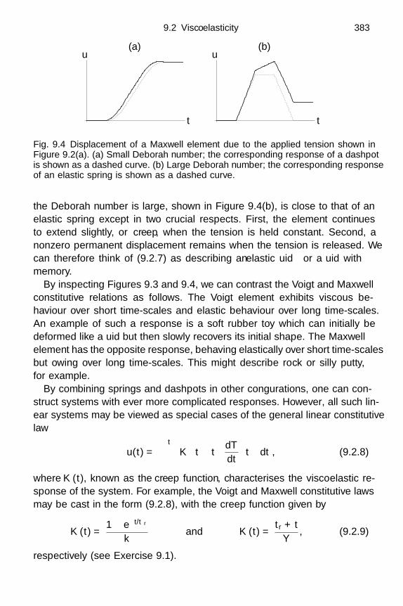
9.2 Viscoelasticity 383
u(a)
t
u(b)
t
Fig. 9.4 Displacement of a Maxwell element due to the applied tension shown inFigure 9.2(a). (a) Small Deborah number; the corresponding response of a dashpotis shown as a dashed curve. (b) Large Deborah number; the corresponding responseof an elastic spring is shown as a dashed curve.
the Deborah number is large, shown in Figure 9.4(b), is close to that of anelastic spring except in two crucial respects. First, the element continuesto extend slightly, or creep, when the tension is held constant. Second, anonzero permanent displacement remains when the tension is released. Wecan therefore think of (9.2.7) as describing an elastic fluid or a fluid withmemory.
By inspecting Figures 9.3 and 9.4, we can contrast the Voigt and Maxwellconstitutive relations as follows. The Voigt element exhibits viscous be-haviour over short time-scales and elastic behaviour over long time-scales.An example of such a response is a soft rubber toy which can initially bedeformed like a fluid but then slowly recovers its initial shape. The Maxwellelement has the opposite response, behaving elastically over short time-scalesbut flowing over long time-scales. This might describe rock or silly putty,for example.
By combining springs and dashpots in other configurations, one can con-struct systems with ever more complicated responses. However, all such lin-ear systems may be viewed as special cases of the general linear constitutivelaw
u(t) =∫ t
−∞K(t − t′
) dT
dt
(t′)
dt′, (9.2.8)
where K(t), known as the creep function, characterises the viscoelastic re-sponse of the system. For example, the Voigt and Maxwell constitutive lawsmay be cast in the form (9.2.8), with the creep function given by
K(t) =1 − e−t/tr
kand K(t) =
tr + t
Y , (9.2.9)
respectively (see Exercise 9.1).
384 More general theories
We point out that one-dimensional linear viscoelasticity can be approachedby generalising Exercise 1.3 and taking the continuum limit of a series ofspring and dashpot elements. Some of the different possibilities are describedin Exercise 9.2.
9.2.3 Three-dimensional linear viscoelasticity
When constructing the constitutive relationship for a linear elastic mediumin Chapter 1, we supposed that each infinitesimal line element in the materialobeys a version of Hooke’s law. Now we can incorporate viscoelastic effectsby replacing Hooke’s law with a rate-dependent constitutive law such as(9.2.4) or (9.2.7). There is no hard-and-fast rule for doing this: for any givenmaterial the choice of constitutive law must be based on its qualitativeproperties, for example whether it behaves like a fluid or a solid over shortand long time-scales, and must then be verified experimentally.
The Voigt element Figure 9.1(c), for example, could be generalised to threedimensions as follows. We imagine that the stress tensor τij at each pointis provided by an elastic contribution τ e
ij and a viscous contribution τvij . We
then assume that these satisfy the standard linear elastic and Newtonianconstitutive relations, so that
τij = τ eij + τv
ij , τ eij = λ (ekk) δij + 2µeij , τv
ij = ξ (Dkk) δij + 2ηDij ,
(9.2.10)
where λ and µ are the usual Lame constants, while ξ and η are calledthe dilatational viscosity and shear viscosity respectively. As explained inSection 8.8, the rate-of-strain tensor Dij may be approximated as simply thetime derivative of the strain tensor eij provided the displacement gradientsare small enough for linear elasticity to be valid.
If we make the simplifying assumption that the elastic and viscous com-ponents have the same Poisson’s ratio, then we can define a single relaxationtime
tr =ξ
λ=
η
µ. (9.2.11)
Then, by collecting the terms in (9.2.10), we obtain the constitutive relation
τij =(
1 + tr∂
∂t
)(λ (ekk) δij + 2µeij) , (9.2.12)
for small displacements of a Voigt solid.Alternatively, we can base a Maxwell model on the idea that the stress
at any point gives rise to both an elastic strain eeij and a viscous strain ev
ij .
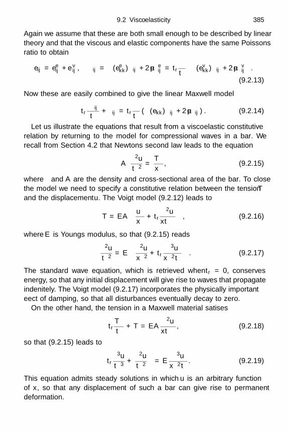
9.2 Viscoelasticity 385
Again we assume that these are both small enough to be described by lineartheory and that the viscous and elastic components have the same Poisson’sratio to obtain
eij = eeij + ev
ij , τij = λ (eekk) δij + 2µee
ij = tr∂
∂t
(λ (ev
kk) δij + 2µevij
).
(9.2.13)
Now these are easily combined to give the linear Maxwell model
tr∂τij
∂t+ τij = tr
∂
∂t(λ (ekk) δij + 2µeij) . (9.2.14)
Let us illustrate the equations that result from a viscoelastic constitutiverelation by returning to the model for compressional waves in a bar. Werecall from Section 4.2 that Newton’s second law leads to the equation
ρA∂2u
∂t2=
∂T
∂x, (9.2.15)
where ρ and A are the density and cross-sectional area of the bar. To closethe model we need to specify a constitutive relation between the tension T
and the displacement u. The Voigt model (9.2.12) leads to
T = EA
(∂u
∂x+ tr
∂2u
∂x∂t
), (9.2.16)
where E is Young’s modulus, so that (9.2.15) reads
ρ∂2u
∂t2= E
(∂2u
∂x2 + tr∂3u
∂x2∂t
). (9.2.17)
The standard wave equation, which is retrieved when tr = 0, conservesenergy, so that any initial displacement will give rise to waves that propagateindefinitely. The Voigt model (9.2.17) incorporates the physically importanteffect of damping, so that all disturbances eventually decay to zero.
On the other hand, the tension in a Maxwell material satisfies
tr∂T
∂t+ T = EA
∂2u
∂x∂t, (9.2.18)
so that (9.2.15) leads to
ρ
(tr
∂3u
∂t3+
∂2u
∂t2
)= E
∂3u
∂x2∂t. (9.2.19)
This equation admits steady solutions in which u is an arbitrary functionof x, so that any displacement of such a bar can give rise to permanentdeformation.
386 More general theories
More generally, we can think of (9.2.12) and (9.2.14) as special cases ofthe general linear three-dimensional constitutive relation
eij =∫ t
−∞Kijk
(t − t′
) ∂τk
∂t
(x, t′
)dt′, (9.2.20)
where the creep function is now in general a fourth-rank tensor. If the ma-terial is isotropic, then (9.2.20) may be characterised using just two scalarcreep functions L(t) and M(t) by writing
eij =∫ t
−∞
L(t − t′
) ∂τkk
∂t
(x, t′
)δij + M
(t − t′
) ∂τij
∂t
(x, t′
)dt′.
(9.2.21)In either case, the integral should really be performed with the Lagrangianvariable X held fixed, and we must emphasise once more that all theselinear theories are only valid for small strains. We can expect them to workwell for small displacements of a damped solid or for small creep of anelastic fluid, but for a fluid that undergoes a substantial deformation, amore sophisticated approach is required, as we will now briefly explain.
9.2.4 Large-strain viscoelasticity
In viscoelastic fluids, the strains are frequently so large that, as in Chap-ter 5, we must resort to Lagrangian variables to deal with the geometricnonlinearity. While such materials may undergo large deformations, theircompressibility is nearly always small in comparison, and it is thereforeusual to model them as incompressible. We therefore introduce a pressure p
and a deviatoric stress τ ′, as in Section 8.4.3, so that Cauchy’s momentumequation takes the form
ρ
∂v
∂t+ (v · ∇)v
= −∇p + ∇ · τ ′ + ρg, (9.2.22)
where v is the velocity vector.Since we would not expect a Voigt solid to undergo particularly large
displacements, we concentrate on the example of a Maxwell fluid, in whichthe deformation is decomposed into an elastic component and a viscouscomponent. As described in any book on viscous flow (for example Ockendon& Ockendon, 1995), the constitutive relation for a Newtonian viscous fluidis simply
τ ′ij = 2ηDij , (9.2.23)
where Dij is the rate-of-strain tensor and η is again the shear viscosity.

9.2 Viscoelasticity 387
On the other hand, a neo-Hookean solid, with strain energy density givenby (5.3.58a), obeys the constitutive relation
τ ′ij = µ (Bij − δij) , (9.2.24)
where the Finger strain tensor Bij is defined in (5.2.14). By differentiatingthe Finger tensor with respect to t, as shown in Exercise 9.4, we find that
DBij
Dt=
∂vi
∂xkBkj + Bik
∂vj
∂xk, (9.2.25)
that isDBDt
= ∇vTB + B∇v, (9.2.26)
where D/Dt = ∂/∂t + (v · ∇) is the “usual” convective derivative.The neo-Hookean stress tensor (9.2.24) therefore satisfies the equation
τ ′ = 2µD, (9.2.27)
where
denotes the upper convected derivative, defined for an arbitrarytensor function A by
A =DA
Dt− ∇vTA − A∇v. (9.2.28)
By combining (9.2.23) and (9.2.27), a viscoelastic fluid whose elastic com-ponent is neo-Hookean could be described by
tr
τ ′ + τ ′ = 2ηD, (9.2.29)
which is known as the upper convected Maxwell model.As another example of an elastic constitutive relation, let us consider the
Mooney–Rivlin strain energy density (5.3.58b), with c1 = 0, c2 = µ/2, whichleads to
τ ′ij = µ
(δij − B−1
ij
). (9.2.30)
Again using (9.2.25), we discover that this stress tensor satisfies
τ ′ = 2µD, (9.2.31)
where the lower convected derivative of a tensor A is defined by
A =DA
Dt+ ∇vA + A∇vT. (9.2.32)
We obtain the lower convected Maxwell model by using
instead of
in(9.2.28).
388 More general theories
Both
and
are special cases of a one-parameter family of convectedderivatives, defined by
A =
DA
Dt− ΩA + AΩ − a (DA + AD) , (9.2.33)
where Ω is the rotation tensor, that is
Ωij =12
(∂vi
∂xj− ∂vj
∂xi
). (9.2.34)
The upper and lower convected derivatives are obtained when a = 1 andwhen a = −1 respectively, and another common choice is the Jaumann
or corotational derivativeA, corresponding to a = 0. In any viscoelastic
constitutive relation, a is a material parameter that must be determinedfrom experiments.
For any value of a, the derivative defined by (9.2.33) is objective. By thiswe mean that it is invariant under rigid-body transformations, and cruciallythis includes unsteady transformations. This means that it is the same for allobservers, in contrast with the usual convective derivative DA/Dt. Hence,when we construct a constitutive relation using
, we can be sure that the
resulting mechanical behaviour will be independent of the frame in whichit is measured. Nonetheless, whichever member of (9.2.33) we choose, theresulting large-strain viscoelastic model will couple (9.2.22) with an equallycomplicated nonlinear evolution equation for τ ′. Hence analytical progresscan usually only be made in the case of small strains, in which case
is
approximately ∂/∂t.Finally, we must mention that the identification and classification of con-
vective derivatives of tensors is one that arises in many branches of mathe-matics, and it is interesting that these derivatives have a geometrical inter-pretation, as shown in Exercise 9.5.
9.3 Thermoelasticity
Thermal effects in solids can be dramatic, even if we exclude the possibility ofthe solid melting into a liquid. For example, the easiest way in which to frac-ture an ice cube is to put it into even lukewarm water. We note that densityvariations are already allowed for in the mass- and momentum-conservationequations (1.3.6) and (1.6.5). Hence it only remains for us to incorporatethermal effects in the constitutive equation (1.7.6) and then to include heatin the energy calculation from Section 1.9. We will assume throughout thatthe displacement gradients are small enough for linear elasticity to be valid.

9.3 Thermoelasticity 389
We begin to construct a linear thermoelastic constitutive relation by con-sidering an unconstrained elastic solid whose absolute temperature is raisedfrom T0 in the reference state to a new temperature T . There is ample exper-imental evidence that many common materials undergo a uniform isotropicvolume change, namely an expansion if T > T0 or a contraction if T < T0.For moderate temperature variations, the thermal expansion is found to varylinearly with temperature, so that
eij =α
3(T − T0)δij , (9.3.1)
where α is called the coefficient of thermal expansion. By referring to Sec-tion 2.2.1, we can interpret α as the relative volume expansion caused by aunit increase in temperature.
We are therefore prompted to propose the constitutive relation
τij = 2µeij + λekkδij −(
λ +23µ
)α(T − T0)δij . (9.3.2)
This is the only linear relation between τij , eij and T which reduces to(1.7.6) when T = T0 and to (9.3.1) when τij = 0. In a linear theory, theLame constants are assumed not to vary significantly over the temperatureranges of interest. When we use (9.3.2) in the momentum equation (1.6.5),we find that the Navier equation generalises to
ρ∂2u
∂t2= ρg + (λ + µ) grad div u + µ∇2u −
(λ +
23µ
)α∇T, (9.3.3)
so that the temperature gradient generates an effective body force in theNavier equation.
At first glance, it might appear from (9.3.3) that a uniform temperaturechange, with ∇T = 0, could not drive a displacement. However, wheneverboundary conditions are specified on the displacement, the constitutive re-lation (9.3.2) will lead to nontrivial stress, and vice versa. We illustrate thisby returning to the steady uniaxial loading of a bar, considered previouslyin Section 2.2.3. Here we examine the effect of heating the bar uniformly tosome temperature T . If we seek a displacement of the form
u = (βx,−γy,−γz)T , (9.3.4)
then the stress tensor is given by (9.3.2) as
τ = 2µ
β 0 00 −γ 00 0 −γ
+[λ(β − 2γ) −
(λ +
2µ
3
)α(T − T0)
]I. (9.3.5)

390 More general theories
By ensuring that the lateral stress components τyy and τzz are zero, we findthat the transverse strain is given by
γ =λβ
2(λ + µ)− (3λ + 2µ)α(T − T0)
6(λ + µ)= νβ − 1 + ν
3α(T − T0), (9.3.6)
where ν is Poisson’s ratio. The only remaining nonzero stress component is
τxx =(
β − 13α(T − T0)
)E, (9.3.7)
where E is Young’s modulus.We can use this result to calculate the thermal stress in a length of railway
track.† If the two ends of the track are fixed, then we must have β = 0, andhence the net compressive force is given by
P =EA
3α(T − T0), (9.3.8)
where A is the cross-sectional area. Note that heating the track will cause acompressive force and cooling a tensile force, as expected. From Section 4.4.3,we know that the track will buckle if the compressive stress is too large, and(9.3.8) tells us that the maximum temperature that can be sustained beforebuckling occurs is
T − T0 =3π2I
AL2α, (9.3.9)
where I is the moment of inertia of the cross-section.In general, we cannot assume that temperature is known, but must de-
termine it as part of the solution. We now obtain an equation for T byperforming an energy balance. The net energy U in a control volume V isgiven by
U =∫∫∫
V
12ρ
∣∣∣∣∂u
∂t
∣∣∣∣2 + W + ρcT
dx, (9.3.10)
where, referring to Section 1.9, we recognise the first two terms in the inte-grand as the kinetic energy and the strain energy. The final term is the ther-mal energy, with c denoting the specific heat capacity,‡ a material parameterwhich we will assume to be constant. As in Section 8.7 and Exercise 8.12,the first law of thermodynamics tells us that all three forms of energy are
†In the days before “continuously-welded” rails, gaps had to be left between sections of track toallow for thermal expansion to take place without stress generation. These gaps caused trackand wheels to wear and led to many accidents.‡As usual, this should be defined “at constant volume”

9.4 Composite materials and homogenisation 391
equivalent and mutually convertible. However, in contrast with Section 8.7,our solid now has a strain energy density W such that τij = ∂W/∂eij .
The energy inside V will change due to the work done by gravity, the workdone by stress on the boundary ∂V , and the flux of heat through ∂V . Col-lecting these effects together, we arrive at the energy conservation equation
dU
dt=∫∫∫
Vρg · ∂u
∂tdx +
∫∫∂V
(τn) · ∂u
∂tda −
∫∫∂V
q · n da, (9.3.11)
where n is the unit normal to ∂V and q is the heat flux. Now we haveto substitute (9.3.10) into (9.3.11) and simplify the resulting expression.As shown in Exercise 9.7, for sufficiently small temperature variations, thisleads to
ρc∂T
∂t+ div q = 0, (9.3.12)
which is the standard equation for heat flow in a rigid sample. In otherwords, there is no leading-order coupling between thermal expansion andheat flow: we can solve (9.3.12) for T and then substitute the result into(9.3.3) to determine the resulting displacement.
For most materials, the heat flux is given by Fourier’s law, namelyq = −k∇T where k is the thermal conductivity. Provided k is constant,(9.3.12) just becomes the linear heat equation
∂T
∂t= κ∇2T, (9.3.13)
where κ = k/ρc is called the thermal diffusivity. We note in passing that thesituation is much more complicated when thermal radiation is significant,as often happens in semi-transparent materials such as glass.
9.4 Composite materials and homogenisation
9.4.1 One-dimensional homogenisation
Many practically important materials have properties which vary over avery fine scale, for example composites consisting of alternating layers withtwo different properties. To describe deformations of such a material, itis usually impractical to analyse each individual layer. In this section, webriefly outline a homogenisation technique that allows us to average overthe fine scale and hence determine effective mechanical properties for large-scale deformations of the material as a whole. The word homogenisation isoften used synonymously with “multi-scaling” or “coarse-graining”. We willonly consider configurations where the short scale greatly exceeds molecularlength-scales.
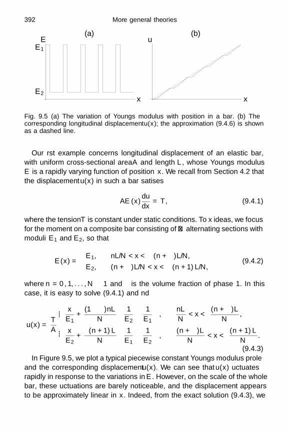
392 More general theories
xx
E uE1
E2
(a) (b)
Fig. 9.5 (a) The variation of Young’s modulus with position in a bar. (b) Thecorresponding longitudinal displacement u(x); the approximation (9.4.6) is shownas a dashed line.
Our first example concerns longitudinal displacement of an elastic bar,with uniform cross-sectional area A and length L, whose Young’s modulusE is a rapidly varying function of position x. We recall from Section 4.2 thatthe displacement u(x) in such a bar satisfies
AE(x)du
dx= T, (9.4.1)
where the tension T is constant under static conditions. To fix ideas, we focusfor the moment on a composite bar consisting of 2N alternating sections withmoduli E1 and E2, so that
E(x) =
E1, nL/N < x < (n + φ)L/N,
E2, (n + φ)L/N < x < (n + 1)L/N,(9.4.2)
where n = 0, 1, . . . , N − 1 and φ is the volume fraction of phase 1. In thiscase, it is easy to solve (9.4.1) and find
u(x) =T
A
x
E1+
(1 − φ)nL
N
(1
E2− 1
E1
),
nL
N< x <
(n + φ)LN
,
x
E2+
φ(n + 1)LN
(1
E1− 1
E2
),
(n + φ)LN
< x <(n + 1)L
N.
(9.4.3)In Figure 9.5, we plot a typical piecewise constant Young’s modulus profile
and the corresponding displacement u(x). We can see that u(x) fluctuatesrapidly in response to the variations in E. However, on the scale of the wholebar, these fluctuations are barely noticeable, and the displacement appearsto be approximately linear in x. Indeed, from the exact solution (9.4.3), we
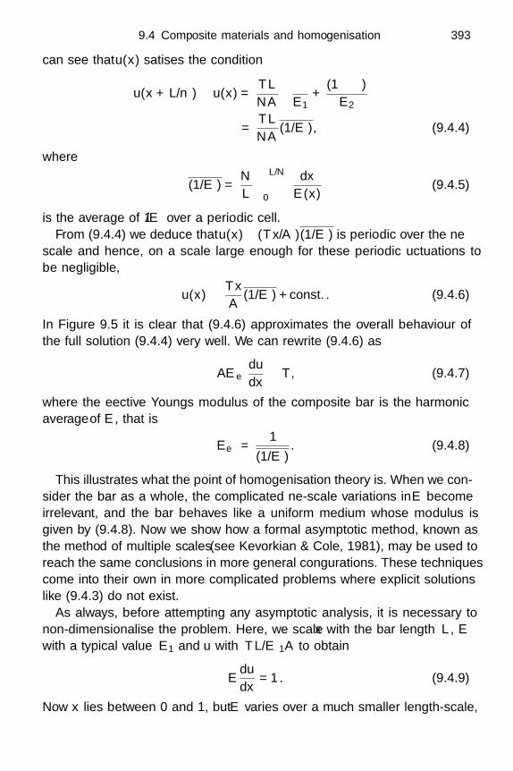
9.4 Composite materials and homogenisation 393
can see that u(x) satisfies the condition
u(x + L/n) − u(x) =TL
NA
(φ
E1+
(1 − φ)E2
)=
TL
NA(1/E), (9.4.4)
where
(1/E) =N
L
∫ L/N
0
dx
E(x)(9.4.5)
is the average of 1/E over a periodic cell.From (9.4.4) we deduce that u(x)− (Tx/A)(1/E) is periodic over the fine
scale and hence, on a scale large enough for these periodic fluctuations tobe negligible,
u(x) ∼ Tx
A(1/E) + const.. (9.4.6)
In Figure 9.5 it is clear that (9.4.6) approximates the overall behaviour ofthe full solution (9.4.4) very well. We can rewrite (9.4.6) as
AEeffdu
dx∼ T, (9.4.7)
where the effective Young’s modulus of the composite bar is the harmonicaverage of E, that is
Eeff =1
(1/E). (9.4.8)
This illustrates what the point of homogenisation theory is. When we con-sider the bar as a whole, the complicated fine-scale variations in E becomeirrelevant, and the bar behaves like a uniform medium whose modulus isgiven by (9.4.8). Now we show how a formal asymptotic method, known asthe method of multiple scales (see Kevorkian & Cole, 1981), may be used toreach the same conclusions in more general configurations. These techniquescome into their own in more complicated problems where explicit solutionslike (9.4.3) do not exist.
As always, before attempting any asymptotic analysis, it is necessary tonon-dimensionalise the problem. Here, we scale x with the bar length L, E
with a typical value E1 and u with TL/E1A to obtain
Edu
dx= 1. (9.4.9)
Now x lies between 0 and 1, but E varies over a much smaller length-scale,
394 More general theories
of order ε, say. We therefore write E in the form
E = E (x, ξ) , (9.4.10)
where ξ = x/ε and E is assumed to be periodic, with period one, withrespect to its second argument. In our example (9.4.2), ε = 1/N and E
depends only on the fine scale ξ. Here we allow E also to vary on the scaleof the whole bar, for example if we had allowed E1 and E2 in (9.4.2) to varyslowly with x.
With E given by (9.4.10), we must now take u to be a function of thetwo length-scales x and ξ; this means that we have moved from a modelthat is one-dimensional in the variable x to one that is two-dimensional inthe plane (x, ξ). However, physical space is just the line x = εξ in the (x, ξ)plane, and on this line the chain rule implies that
du
dx=
∂u
∂x+
1ε
∂u
∂ξ. (9.4.11)
Hence (9.4.9) becomes
E(x, ξ)(
∂u
∂ξ+ ε
∂u
∂x
)= ε. (9.4.12)
To obtain a unique representation of u in terms of x and ξ, we insist that u,like E, must be periodic with respect to ξ.†
Now we take the limit ε → 0 and seek the solution as an asymptoticexpansion of the form u ∼ u0 + εu1 + · · · . When we equate terms of O (1),we discover that
∂u0
∂ξ= 0, (9.4.13)
so that u0 is a function of x alone, and then, at order ε,
E(x, ξ)(
∂u1
∂ξ+
du0
dx
)= 1. (9.4.14)
The assumed periodicity of u with respect to ξ leads to the condition
Eeff(x)du0
dx= 1, (9.4.15)
where
Eeff(x) = 1/∫ 1
0
dξ
E(x, ξ)
=
1(1/E)
. (9.4.16)
†This is a very convenient assumption but, as discussed in Kevorkian & Cole (1981), it is notnecessary for more general problems in which the micro-geometry is not known in advance,and can be replaced by the condition that u not grow as |ξ| → ∞.

9.4 Composite materials and homogenisation 395
xx
E uE1
E2
(a) (b)
Fig. 9.6 (a) The variation of Young’s modulus with position in a bar with ε = 1/5;the effective Young’s modulus is shown as a dashed curve. (b) The correspondinglongitudinal displacement u(x); the leading-order approximation, given by (9.4.15),is shown as a dashed curve.
This is equivalent to (9.4.8) when E depends on ξ alone, but (9.4.16) allowsfor E also to vary slowly with x.
To illustrate this result, let us return to the piecewise constant example(9.4.2), but now allow E1 and E2 to be functions of x. In terms of dimen-sionless variables, we can therefore write E as a periodic function of ξ givenby
E(x, ξ) =
E1(x), 0 < ξ < φ,
E2(x), φ < ξ < 1.(9.4.17)
We show a typical example in Figure 9.6(a), along with the effective modulus
Eeff(x) =∫ 1
0
dξ
E(x, ξ)
−1
=E1(x)E2(x)
(1 − φ)E1(x) + φE2(x), (9.4.18)
which averages out the fine scale variations. We see in Figure 9.6(b) that thedisplacement calculated using Eeff(x) (dashed curve) provides an excellentapproximation to the exact solution (solid curve), even though ε = 1/5 isnot particularly small.
9.4.2 Two-dimensional homogenisation
Let us now consider a less trivial application of this method, namely an-tiplane strain in a bar whose shear modulus µ varies over the cross-section.It is straightforward, following the ideas of Section 2.3, to see that, in suit-able dimensionless variables, the axial displacement w(x, y) satisfies
∇ · (µ∇w) = 0. (9.4.19)

396 More general theories
ηµ2
µ1
b
ξ 1
Fig. 9.7 A periodic microstructured shear modulus.
We suppose that µ varies both rapidly over a short length-scale ε and grad-ually across the whole cross-section, so that we can write
µ = µ(x, y, ξ, η), (9.4.20)
where (ξ, η) = (x, y)/ε. We also assume that µ is periodic in both directionsover the fine scale, so that
µ(x, y, ξ + 1, η) ≡ µ(x, y, ξ, η), µ(x, y, ξ, η + b) ≡ µ(x, y, ξ, η). (9.4.21)
We choose ε such that the period in ξ is equal to 1, and then define b to be theperiod in the η-direction. A typical setup is illustrated in Figure 9.7, wherethe modulus µ is piecewise constant on the fine scale, although µ1(x, y) andµ2(x, y) might vary over the long scale.
Now, as in Section 9.4.1, we allow the displacement field w(x, y, ξ, η) tovary over both length-scales, provided it shares the same periodicity (9.4.21)as µ. The chain rule thus transforms (9.4.19) into
∇ξ · (µ∇ξw) + ε ∇ξ · (µ∇xw) + ∇x · (µ∇ξw) + ε2∇x · (µ∇xw) = 0,
(9.4.22)where ∇x = (∂/∂x, ∂/∂y)T, ∇ξ = (∂/∂ξ, ∂/∂η)T. The assumed periodicitymeans that we need only solve (9.4.22) on a single rectangular cell [0, 1]×[0, b]
9.4 Composite materials and homogenisation 397
and then apply the periodic boundary conditions
w(x, y, 1, η) ≡ w(x, y, 0, η), w(x, y, ξ, b) ≡ w(x, y, ξ, 0), (9.4.23a)∂w
∂ξ(x, y, 1, η) ≡ ∂w
∂ξ(x, y, 0, η),
∂w
∂η(x, y, ξ, b) ≡ ∂w
∂η(x, y, ξ, 0). (9.4.23b)
When we again seek the solution as an asymptotic expansion of the form
w ∼ w0 + εw1 + ε2w2 + · · · , (9.4.24)
we immediately discover that w0 satisfies
∇ξ · (µ∇ξw0) = 0. (9.4.25)
This equation and the boundary conditions (9.4.23) are identically satisfiedif w0 is independent of ξ and η, so that w0 = w0(x, y), and it may be shown(see Exercise 9.10) that this is the only solution. As we might have hoped,the displacement therefore does not vary on the fine length-scale to leadingorder.
Comparing the terms at O (ε), we obtain
∂
∂ξ
(µ
∂w1
∂ξ
)+
∂
∂η
(µ
∂w1
∂η
)= −∂µ
∂ξ
∂w0
∂x− ∂µ
∂η
∂w0
∂y= R1(x, y, ξ, η), say,
(9.4.26)which is a linear elliptic partial differential equation for w1 driven by ∇xw0.As shown in Exercise 9.10, equation (9.4.26) admits periodic solutionsfor w1 only if the right-hand side has zero mean, so that∫ 1
0
∫ b
0R1(x, y, ξ, η) dξdη = 0. (9.4.27)
This requirement is satisfied identically here, and we can write the solutionin the form
w1 = W (1)(x, y, ξ, η)∂w0
∂x+ W (2)(x, y, ξ, η)
∂w0
∂y, (9.4.28)
where W (1) and W (2) satisfy the equations
∂
∂ξ
(µ
∂W (1)
∂ξ
)+
∂
∂η
(µ
∂W (1)
∂η
)= −∂µ
∂ξ(9.4.29)
and∂
∂ξ
(µ
∂W (2)
∂ξ
)+
∂
∂η
(µ
∂W (2)
∂η
)= −∂µ
∂η, (9.4.30)
with the periodic conditions (9.4.23).

398 More general theories
It can be shown that (9.4.29) and (9.4.30) have unique periodic solutionsfor W (1) and W (2), up to arbitrary additive functions of (x, y). Although itis usually not possible to obtain these solutions in closed form, it is straight-forward in principle to compute them numerically for any given modulusfunction µ(x, y, ξ, η).
Finally, proceeding to the terms of O(ε2)
in (9.4.22), we find that w2
satisfies an equation analogous to (9.4.26), but with the right-hand sidereplaced by
R2(x, y, ξ, η) = −
∂
∂ξ
(µ
∂w1
∂x
)+
∂
∂η
(µ
∂w1
∂y
)−
∂
∂x
(µ
∂w1
∂ξ
)+
∂
∂y
(µ
∂w1
∂η
)−
∂
∂x
(µ
∂w0
∂x
)+
∂
∂y
(µ
∂w0
∂y
), (9.4.31)
and again we need this to have zero mean over our periodic cell in (ξ, η).The first term satisfies this requirement identically, and, when we substitutefor w1 from (9.4.28), we find that
0 =∫ 1
0
∫ b
0R2(x, y, ξ, η) dξdη
= −∫ 1
0
∫ b
0
∂
∂x
[µ
(∂W (1)
∂ξ+ 1
)∂w0
∂x+ µ
∂W (2)
∂ξ
∂w0
∂y
]
+∂
∂y
[µ
∂W (1)
∂η
∂w0
∂x+ µ
(∂W (1)
∂η+ 1
)∂w0
∂y
]dξdη. (9.4.32)
Thus our homogenised displacement w0(x, y) satisfies the anisotropic model
∂
∂x
(µ11
∂w0
∂x
)+
∂
∂x
(µ12
∂w0
∂y
)+
∂
∂y
(µ21
∂w0
∂x
)+
∂
∂y
(µ22
∂w0
∂y
)= 0,
(9.4.33)where
µ11 =∫ b
0
∫ 1
0µ
(1 +
∂W (1)
∂ξ
)dξdη, µ21 =
∫ b
0
∫ 1
0µ
∂W (1)
∂ηdξdη,
(9.4.34a)
µ22 =∫ b
0
∫ 1
0µ
(1 +
∂W (2)
∂η
)dξdη, µ12 =
∫ b
0
∫ 1
0µ
∂W (2)
∂ξdξdη.
(9.4.34b)

9.4 Composite materials and homogenisation 399
Thankfully, (9.4.33) can be shown to be elliptic. Equally reassuringly, whenµ is independent of ξ, we can take W (1) = 0 and ∂W (2)/∂ξ = 0, so that
∂W (2)
∂η=
b
µ
∫ b
0
dη
µ
− 1. (9.4.35)
Hence the effective moduli are given by
µ11 =∫ b
0µdη, µ21 = µ12 = 0, µ22 = b2
/∫ b
0
dη
µ, (9.4.36)
which is a generalisation of (9.4.16).For truly two-dimensional geometries, it is almost never possible to eval-
uate the effective moduli explicitly. One famous example where significantprogress can be made occurs when the shear modulus µ is piecewise con-stant, taking one value µ2 on some region D2 inside our rectangular cell,and another value µ1 in the complementary region D1 = [0, 1] × [0, b] \ D2.
When we make the substitutions
φ(1) = W (1) + ξ, φ(2) = W (2) + η, (9.4.37)
the equations (9.4.29) and (9.4.30) for W (1) and W (2) are transformed to
∇ξ ·(µ∇ξφ
(1))
= ∇ξ ·(µ∇ξφ
(2))
= 0, (9.4.38)
where
µ =
µ1, (ξ, η) ∈ D1,
µ2, (ξ, η) ∈ D2.(9.4.39)
Hence φ(1) and φ(2) both satisfy Laplace’s equation in each of D1 and D2,along with the continuity conditions[
φ(j)]
=
[µ
∂φ(j)
∂n
]= 0 (9.4.40)
on the boundary ∂D2 between them.Crucially, we now assume that the geometry possesses reflectional sym-
metry in both the ξ- and the η-direction. Using this symmetry and the pe-riodicity of W (j), we deduce that φ(j) must satisfy the boundary conditions
φ(1)(0, η) = 0, φ(1)(1, η) = 1,∂φ(1)
∂η(ξ, 0) =
∂φ(1)
∂η(ξ, b) = 0, (9.4.41a)
φ(2)(ξ, 0) = 0, φ(2)(ξ, b) = b,∂φ(2)
∂ξ(0, η) =
∂φ(2)
∂ξ(1, η) = 0, (9.4.41b)
as illustrated in Figure 9.8(a).

400 More general theories
(a) (b)
b
∂φ(2)
∂ξ=0
φ(1) =0
η
µ1
D1
D2
µ2
∂D2
∂φ(2)
∂ξ=0
φ(1) =1
∂φ(1)
∂η=0
φ(2) =b
φ(2) =0∂φ(1)
∂η=0
1ξ
η
1ξ
∂ψ(2)
∂η=0
∂ψ(1)
∂ξ=0
ψ(1) =0∂ψ(2)
∂η=0
∂ψ(1)
∂ξ=0
ψ(2) =0
ψ(1) =β
ψ(2) =α
Fig. 9.8 A symmetric, piecewise constant shear modulus distribution; the symmetryaxes are shown as dot-dashed lines. (a) The boundary conditions satisfied by φ(1)
and φ(2) . (b) The corresponding boundary conditions for the harmonic conjugatefunctions ψ(1) and ψ(2) .
Now, since φ(j) satisfy Laplace’s equation in each separate region, we canintroduce the harmonic conjugates ψ(j) which satisfy the Cauchy–Riemannequations
∂φ(j)
∂ξ=
∂ψ(j)
∂η,
∂φ(j)
∂η= −∂ψ(j)
∂ξ. (9.4.42)
The continuity conditions (9.4.40) for φ(j) are transformed to
[µψ(j)
]=
[∂ψ(j)
∂n
]= 0, (9.4.43)
where[ ]
again denotes the jump across ∂D2. The boundary conditions(9.4.41) become
ψ(1)(ξ, 0) = 0, ψ(1)(ξ, b) = β,∂ψ(1)
∂ξ(0, η) =
∂ψ(1)
∂ξ(1, η) = 0, (9.4.44a)
ψ(2)(0, η) = 0, ψ(2)(1, η) = α,∂ψ(2)
∂η(ξ, 0) =
∂ψ(2)
∂η(ξ, b) = 0, (9.4.44b)
as shown in Figure 9.8(b), where the constants α and β are unknown inadvance.
It is straightforward to calculate the effective elastic constants using ψ(j),because the continuity conditions (9.4.43) allow us to integrate directly

9.4 Composite materials and homogenisation 401
across the cell. For example,
µ11 =∫ b
0
∫ 1
0µ
∂φ(1)
∂ξdξdη =
∫ b
0
∫ 1
0µ
∂ψ(1)
∂ηdξdη
=∫ 1
0
[µψ(1)
]η=b
η=0dξ = µ1β, (9.4.45)
and analogous calculations yield
µ22 = −µ1bα, µ21 = µ12 = 0, (9.4.46)
so the assumed symmetry of the geometry eliminates the off-diagonal terms.Now the key observation is that the problem satisfied by ψ(2) closely
resembles that for φ(1) (and vice versa). Indeed, if we define
φ(1) =µ2ψ
(2)
αµ1, (9.4.47)
then the boundary conditions for φ(1) are identical to (9.4.41a), althoughthe continuity conditions on ∂D2 read
φ(1)∣∣∣D1
= φ(1)∣∣∣D2
, µ2∂φ(1)
∂n
∣∣∣∣∣D1
= µ1∂φ(1)
∂n
∣∣∣∣∣D2
. (9.4.48)
Hence φ(1) is what φ(1) would be if we switched the values of µ1 and µ2. Wecan use the same technique as above to calculate the corresponding elasticconstants, noting that the harmonic conjugate of φ(1) is
ψ(1) = −µ2φ(2)
αµ1, (9.4.49)
so that
µ11 = µ2
[ψ(1)
]η=b
η=0= −µ2b
α. (9.4.50)
Eliminating α between (9.4.46) and (9.4.50), we obtain the intriguingrelation
µ11µ22 = b2µ1µ2 (9.4.51)
between the stiffness µ22 in the η-direction and the corresponding stiffnessµ11 in the ξ-direction with µ1 and µ2 switched. This has particularly startlingimplications if b = 1 and the geometry is anti-symmetric about a diagonalin the resulting square cell, as in the examples shown in Figure 9.9. In suchconfigurations, swapping µ1 and µ2 is equivalent to swapping ξ and η, so
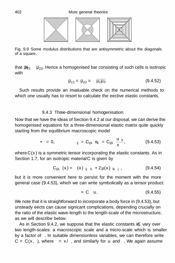
402 More general theories
Fig. 9.9 Some modulus distributions that are antisymmetric about the diagonalsof a square.
that µ11 ≡ µ22. Hence a homogenised bar consisting of such cells is isotropicwith
µ11 = µ22 =√
µ1µ2. (9.4.52)
Such results provide an invaluable check on the numerical methods towhich one usually has to resort to calculate the effective elastic constants.
9.4.3 Three-dimensional homogenisation
Now that we have the ideas of Section 9.4.2 at our disposal, we can derive thehomogenised equations for a three-dimensional elastic matrix quite quicklystarting from the equilibrium macroscopic model
∇ · τ = 0, τij = Cijkek = Cijk∂uk
∂x, (9.4.53)
where C(x) is a symmetric tensor incorporating the elastic constants. As inSection 1.7, for an isotropic material C is given by
Cijk(x) = λ(x)δijδk + 2µ(x)δikδj, (9.4.54)
but it is more convenient here to persist for the moment with the moregeneral case (9.4.53), which we can write symbolically as a tensor product:
τ = C∇u. (9.4.55)
We note that it is straightforward to incorporate a body force in (9.4.53), butunsteady effects can cause significant complications, depending crucially onthe ratio of the elastic wave-length to the length-scale of the microstructure,as we will describe below.
As in Section 9.4.2, we suppose that the elastic constants in C vary overtwo length-scales: a macroscopic scale and a micro-scale which is smallerby a factor of ε. In suitable dimensionless variables, we can therefore writeC = C(x, ξ), where ξ = x/ε, and similarly for u and τ . We again assume
9.4 Composite materials and homogenisation 403
that C, u and τ are all periodic on some representative cell D, for examplea cuboid, in ξ-space.
The advantage of working with the first-order system (9.4.53), rather thanthe Navier equations, is that when we expand
u ∼ u0(x, ξ) + εu1(x, ξ) + · · · , τ ∼ τ0(x, ξ) + ετ1(x, ξ) + · · · , (9.4.56)
we only need to consider terms up to O (ε), in contrast with Section 9.4.2where we had to proceed to O
(ε2).
At leading order, we soon find that
∇ξ · τ0 = 0, (9.4.57)
C∇ξu0 = 0, (9.4.58)
the second of which implies that u0 is a rigid body motion as a functionof ξ, and our assumed periodicity implies that
u0 = u0(x), (9.4.59)
as in (9.4.25). At order ε, we obtain the equations
∇ξ · τ1 + ∇x · τ0 = 0, (9.4.60)
τ0 = C∇ξu1 + C∇xu0. (9.4.61)
If we operate with ∇ξ on (9.4.61) then, by virtue of (9.4.57), we obtain alinear problem for u1, namely
∇ξ · (C∇ξu1) = − (∇ξ · C) (∇xu0) , (9.4.62)
which is driven by a term proportional to ∇xu0. Hence, as in (9.4.28), wecan formally write u1 in the form
u1 = A(x, ξ)∇xu0, (9.4.63)
where A = (Aijk) is rank-three tensor which in principle is determinedby solving (9.4.62); usually this will have to be done numerically. Back-substitution into (9.4.61), as demonstrated in Exercise 9.12, gives that τ0(x, ξ)is related to u0 by
τ0 = (C∇ξA) ∇xu0 + C∇xu0. (9.4.64)
As always, the final step is to demand that τ be periodic on our unit cellD. This means that ∫∫∫
D∇ξ · τ1 dξ ≡ 0, (9.4.65)

404 More general theories
and we therefore deduce from (9.4.60) that
∇x · τ 0 = 0, (9.4.66)
where τ 0 again denotes the average of τ0 over D. Hence, on the macroscopicscale, the leading-order displacement u0 satisfies the homogenised equation
∇x · (Ceff∇xu0) = 0, where Ceff(x) = (C∇ξA + C). (9.4.67)
We remark again that the effective elastic constants can rarely be evalu-ated explicitly, although, for any given microstructure, they can in principlebe calculated numerically over a representative unit cell. Another crucialobservation is that, even if the matrix is constructed from isotropic mate-rial, so that C is given by (9.4.54), the averaging will in general lead toan anisotropic macroscopic constitutive law. Of course, most natural het-erogeneous media do not have a regular periodic microstructure. For suchmaterials, we must view D as a representative cell that is characteristic ofthe medium as a whole. Unless the microstructure has a particular direction-ality, we might expect a random geometry to lead to isotropic macroscopicbehaviour.
9.4.4 Waves in periodic media
We conclude this section with a short discussion of waves in composite me-dia. Unfortunately, the multiple reflections, refractions and diffractions thatcan occur make the theory much more complicated than in the static casesconsidered above. However, it is very similar to the theory of electromag-netic wave propagation through lattices, which underpins much of solid statephysics, so we will illustrate the basic ideas by considering one-dimensionalmotion of an elastic bar.
The generalisation of (4.2.4) to an inhomogeneous bar is
∂
∂x
(E(x)
∂u
∂x
)= ρ
∂2u
∂t2. (9.4.68)
When we seek solutions in the frequency domain and non-dimensionalise asin (9.4.10), we obtain the ordinary differential equation
ddx
(E(x, x/ε)
du
dx
)+
k2
ε2 u = 0, (9.4.69)
where
k = ωεL
√ρ
E1=
εL
Λ, (9.4.70)
and Λ represents the typical wave-length of elastic waves in the bar.
9.4 Composite materials and homogenisation 405
The character of the problem depends crucially on the size of k. If thewave-length is the same order as the length of the bar, then k = O (ε) and(9.4.69) may easily be analysed using the same approach as in Section 9.4.1(see Exercise 9.13). Here we focus on the much more interesting case wherethe wave-length is comparable to the microstructure of the medium, so thatk = O (1). For simplicity, we neglect the dependence on the slow length-scale, so that E is a function only of ξ = x/ε, and (9.4.69) takes the form
ddξ
(E(ξ)
du
dξ
)+ k2u = 0. (9.4.71)
We assume as before that E is periodic so that E(ξ + 1) ≡ E(ξ). However,in contrast with Section 9.4.1, u will in general be a nontrivial function of ξ
that does not share the same periodicity.One possible approach to the differential equation (9.4.71) is to use Floquet
theory, as follows. Let u1(ξ) and u2(ξ) be independent solutions of (9.4.71),for example satisfying the initial conditions
u1(0) = 1,du1
dξ(x, 0) = 0, u2(x, 0) = 0,
du2
dξ(0) = 1. (9.4.72)
Using the standard theory of linear ordinary differential equations (see, forexample, Boyce & DiPrima, 2004, Chapter 3), we easily find that the Wron-skian
W = u1du2
dξ− u2
du1
dξ(9.4.73)
satisfies
E(ξ)W (ξ) ≡ const. = 1, (9.4.74)
if we choose our scaling for E such that E(0) = 1.We can write any other solution of (9.4.71) in terms of u1 and u2 as
u(ξ) = Au1(ξ) + Bu2(ξ), (9.4.75)
where A and B are arbitrary constants. The first key observation is thatu(ξ + 1) also satisfies (9.4.71), and hence
u1(ξ + 1) = Au1(ξ) + Bu2(ξ), (9.4.76)
u2(ξ + 1) = Cu1(ξ) + Du2(ξ), (9.4.77)
where
A = u1(1), B =du1
dξ(1), C = u2(1), D =
du2
dξ(1). (9.4.78)

406 More general theories
These coefficients form the elements of the monodromy matrix
M =(
A C
B D
), (9.4.79)
and we deduce from (9.4.74) that det(M) = 1.Now we look for the possibility of waves by seeking solutions u(ξ) such
that u(ξ + 1) ≡ ru(ξ), where r is constant. It is easy to see that this canonly happen if r is one of the eigenvalues r1, r2 of M . Hence we can writethe general solution of (9.4.71) as a linear combination of eλ1 ξP1(ξ) andeλ2 ξP2(ξ), where λ1,2 = log r1,2 and P1,2(ξ) have period 1. Moreover, sincer1r2 = det(M) = 1, the exponents λ1 and λ2 are either purely real, purelyimaginary, or of the form iπ ± log |r|. Whenever λ1,2 have nonzero real part,then u(ξ) grows exponentially as |ξ| → ∞. The effect of the microscale is thusmuch more dramatic than in the static solutions considered in Section 9.4.1.Instead of simply altering the “effective” wave-speed, it may prevent wavesfrom propagating through the medium altogether.
The eigenvalues of M are given by
r1,2 =12
(T ±
√T 2 − 4
), (9.4.80)
where
T = Tr(M) = u1(1) +du2
dξ(1). (9.4.81)
Given the periodic function E(ξ), we can compute T (k) for each value of k bysolving (9.4.71) and (9.4.72) numerically. If |T (k)| < 2 then the roots (9.4.80)are complex with unit magnitude, and hence λ1,2 are pure imaginary. Weinfer that waves can propagate, although they will not in general be periodic,and the corresponding values of k are called the pass bands. The stop bands,in which waves cannot be supported, occur where |T (k)| > 2.
In Figure 9.10 we show the pass and stop bands when the Young’s modulustakes the form
E(ξ) = 1 + δ sin(2πξ). (9.4.82)
The shaded region is the stop band in which |T | > 2. The parameter δ
measures the non-uniformity in E: when δ = 0, we have E ≡ 1 and allwaves are transmitted through the medium without attenuation. When δ
slightly exceeds zero, a narrow stop band appears near k = π, and grows asδ increases.
We can confirm this behaviour by analysing the problem asymptoticallyin the limit δ → 0. As indicated by Figure 9.10, we expect the stop band to

9.4 Composite materials and homogenisation 407
k/π
δ
Fig. 9.10 Dimensionless wave-number k versus non-uniformity parameter δ whenthe Young’s modulus is given by (9.4.82). The stop band is shaded and the asymp-totic approximation (9.4.88) is shown using dashed lines.
be in a neighbourhood of k = π, and we therefore let k = π + δk1 so that(9.4.71) takes the form
ddξ
((1 + δ sin(2πξ)
)du
dξ
)+ (π + δk1)2u = 0. (9.4.83)
Now we can write u1(ξ, δ) and u2(ξ, δ) as asymptotic expansions in powersof δ and thus obtain the leading-order behaviour of T as δ → 0. Unfortu-nately, this involves considerable tedious algebraic manipulation, which isobviated by the method of multiple scales.
As in Section 9.4.1, we seek a solution of (9.4.83) in the form
u(ξ, δ) ∼ u(0)(x, ξ) + δu(1)(x, ξ) + · · · , (9.4.84)
where x = δξ. At leading order in δ, we find the equation
∂2u(0)
∂ξ2 + π2u(0) = 0, (9.4.85)
whose general solution is
u(0)(x, ξ) = A(x) cos(πξ) + B(x) sin(πξ). (9.4.86)
As usual, we must proceed to O (δ) to obtain equations for the amplitude

408 More general theories
functions A and B, and we discover that u(1) satisfies the equation
∂2u(1)
∂ξ2 + π2u(1) = −3π2
2B cos(3πξ) +
3π2
2A sin(3πξ)
− 2π
dB
dx+ k1A +
π
4B
cos(πξ)
+ 2π
dA
dx− π
4A − k1B
sin(πξ). (9.4.87)
The appearance of sin(πξ) and cos(πξ) on the right-hand side of (9.4.87)will give rise to secular terms, proportional to ξ sin(πξ) and ξ cos(πξ),in u(1). To ensure that u(1) remains bounded as |ξ| → ∞, we must there-fore insist that the coefficients in braces be zero. This gives us two coupledlinear differential equations for A(x) and B(x), whose solutions are eitherexponential or sinusoidal, depending on the value of k1. The stop band, inwhich A and B are exponential, occurs when |k1| < π/4, that is when∣∣∣∣kπ − 1
∣∣∣∣ <δ
4. (9.4.88)
In Figure 9.10, we show that this successfully predicts the behaviour of thestop band near δ = 0.
Alas, the generalisation of Floquet theory to describe wave propagationthrough a periodic medium in higher dimensions poses significant additionalmathematical difficulties. Nevertheless, the same basic idea applies, namelythat the ability of the medium to transmit a given wave can be characterisedby analysing a single representative cell, known as a Brillouin zone in thereciprocal lattice (see Brillouin, 2003).
9.5 Poroelasticity
The theory of Section 9.4.3 may be applied, for example, to a solid thattakes the form of a homogeneous elastic matrix in which are embedded manysmall-scale voids or pores. For such a material, the elastic constants Cijk
would be constant in the elastic matrix and zero in the voids. The situationis much more interesting, though, when the pores are sufficiently connectedfor a viscous fluid to pass through them, as in a liquid-filled sponge, for ex-ample. Other important deformable porous media include oil reservoirs andbiological tissue. In principle, one could follow a homogenisation procedureto derive an averaged macroscopic model governing the deformation of sucha medium. However, the need to couple the Navier equations for the solid

9.5 Poroelasticity 409
matrix to the Navier–Stokes equations for the fluid makes this task consider-ably more complicated than any of the examples encountered in Section 9.4,so we will bypass most of the difficulties associated with the fluid dynamics.
We know from (9.4.67) that we can express the elastic contribution to thestress in the form
τe = Ceff∇u, (9.5.1)
where u is the displacement of the medium and Ceff is the matrix of effectiveelastic constants. If the medium is isotropic, then we can write
τe = λeff (∇ · u) I + µeff(∇u + ∇uT) , (9.5.2)
although the effective elastic constants λeff and µeff will be quite differentfrom the Lame constants of the solid material from which the matrix isconstructed.
A detailed analysis of the fluid dynamics would require us to consider theshear and normal stresses set up in the fluid as it moves through the com-plicated pore structure. In order to avoid this complication, we will assumethe well-substantiated Terzaghi principle (see, for example, Fowler, 1997, p.107) that, on a scale of many pore sizes, the stress in the fluid averagesto an isotropic pore pressure P . The net stress in the medium is thusgiven by
τ = −PI + τe (9.5.3)
and the equilibrium Navier equation reads
(λeff + µeff) grad div u + µeff∇2u = ∇P. (9.5.4)
We therefore have a situation similar to thermoelasticity, with the porepressure playing the role of the temperature. The pressure gradient term in(9.5.4) represents the drag exerted by the fluid on the solid matrix.
The average velocity v at which the fluid flows through the pores is gov-erned by Darcy’s law. This is the physically plausible statement that thedifference between the fluid and solid velocities should be proportional tothe pressure gradient. In the context of linear elasticity, we can approxi-mate the velocity of the solid matrix as the Eulerian time derivative of thedisplacement, so that Darcy’s law reads
v =∂u
∂t− k
η∇P, (9.5.5)
where η is the viscosity of the fluid and k is known as the permeabilityof the medium. This law is confirmed by experiments, and the permeability
410 More general theories
is empirically well characterised for many important porous media. It hasthe dimensions of (length)2 and is of order d2, where d is a typical pore ra-dius. It is also possible to derive (9.5.5) from the underlying Navier–Stokesequations via a homogenisation procedure analogous to that used in Sec-tion 9.4.3. For an anisotropic medium, k must be replaced by a positivedefinite permeability tensor.
To close the problem, we must consider conservation of mass. Each rep-resentative cell of the fluid will contain a volume fraction α, say, of fluid,and the corresponding solid fraction is therefore 1−α. We can thus use theapproach of Section 2.2.1 and the result of Exercise 9.15 to calculate therelative volume change due to a displacement u and hence obtain
α = α0 + (1 − α0)∇ · u. (9.5.6)
On the other hand, conservation of mass for the fluid leads to the equation
∂α
∂t+ α0∇ · v = 0. (9.5.7)
By combining these two equations, we find that, as also shown in Exer-cise 9.15,
∇ · v = −1 − α0
α0
∂
∂t(∇ · u) , (9.5.8)
which shows how compression of the matrix forces the fluid to flow.For simplicity, we have neglected the compressibility of the solid and fluid
phases. We emphasise, though, that the matrix as a whole certainly will becompressible; for example, it is quite possible to compress a sponge madeout of incompressible rubber. We have also assumed that α is always closeto its initial value α0, which is consistent with our assumption that linearelasticity is valid, and that the deformation is sufficiently slow for the inertiaterms in the Navier equations to be ignored. Equations (9.5.2)–(9.5.7) thuscomprise the very simplest model that couples elastic deformation to fluidflow.
If we assume that the parameters λeff, µeff, k and η are all constant, thena straightforward cross-differentiation reveals that div u satisfies the lineardiffusion equation:
∂
∂t(div u) =
((λeff + 2µeff) α0k
η
)∇2 (div u) . (9.5.9)
Hence, the effects of elasticity, viscosity and permeability are all collected inthe effective diffusion coefficient
D =(λeff + 2µeff)α0k
η. (9.5.10)

9.5 Poroelasticity 411
V
F
Lx
P = 0
Fig. 9.11 The one-dimensional squeezing of a sponge.
If D is large (in a suitable dimensionless sense), then the left-hand side of(9.5.9) is negligible and the medium behaves like an elastic solid. Increasingthe stiffness of the matrix thus has a similar overall effect to decreasing thefluid viscosity or increasing the permeability.
As a simple illustration, let us consider one-dimensional squeezing of asponge. With u =
(u(x, t), 0, 0
)T and v =(v(x, t), 0, 0
)T, we can combinethe equilibrium equation (9.5.4) and Darcy’s law (9.5.5) to obtain
(λeff + 2µeff)∂2u
∂x2 =∂P
∂x=
η
k
(∂u
∂t− v
). (9.5.11)
In one dimension, the mass-conservation equation (9.5.8) may be integrateddirectly with respect to x, leading to
(1 − α0)∂u
∂t+ α0v = q(t), (9.5.12)
where q(t) represents the net volume flux of both solid and fluid phases. Wecan use (9.5.12) to eliminate v from (9.5.11) and thus find that u satisfies aforced heat equation
∂u
∂t− D
∂2u
∂x2 = q(t), (9.5.13)
where D is again defined by (9.5.10).To fix ideas, let us consider the situation shown in Figure 9.11, where
one end x = 0 of the sponge is held fixed, although fluid is free to flowinto a reservoir at zero pressure, while the other end x = L is squeezed at aconstant velocity −V by an impermeable plunger. This implies the boundaryconditions
u = P = 0 at x = 0,∂u
∂t= v = −V at x = L, (9.5.14)
noting that, in linear elasticity, the motion of the boundary x = L is ne-glected. It follows that q = −V , and (9.5.13) may then readily be solved by
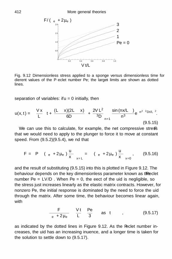
412 More general theories
0.2 0.4 0.6 0.8 1.0
0.5
1.0
1.5
2.0
V t/L
Pe = 0
1
2
3F/(λeff + 2µeff)
Fig. 9.12 Dimensionless stress applied to a sponge versus dimensionless time fordifferent values of the Peclet number Pe; the large-t limits are shown as dottedlines.
separation of variables: if u = 0 initially, then
u(x, t) = −V x
L
(t +
(L − x)(2L − x)6D
)+
2V L2
π3D
∞∑n=1
sin (nπx/L)n3 e−n2 π2 Dt/L2
.
(9.5.15)We can use this to calculate, for example, the net compressive stress F
that we would need to apply to the plunger to force it to move at constantspeed. From (9.5.2)–(9.5.4), we find that
F =[P − (λeff + 2µeff)
∂u
∂x
]x=L
= − (λeff + 2µeff)∂u
∂x
∣∣∣∣x=0
, (9.5.16)
and the result of substituting (9.5.15) into this is plotted in Figure 9.12. Thebehaviour depends on the key dimensionless parameter known as the Pecletnumber Pe = LV/D. When Pe = 0, the effect of the fluid is negligible, sothe stress just increases linearly as the elastic matrix contracts. However, fornonzero Pe, the initial response is dominated by the need to force the fluidthrough the matrix. After some time, the behaviour becomes linear again,with
F
λeff + 2µeff∼ V t
L− Pe
3as t → ∞, (9.5.17)
as indicated by the dotted lines in Figure 9.12. As the Peclet number in-creases, the fluid has an increasing influence, and a longer time is taken forthe solution to settle down to (9.5.17).

9.6 Anisotropy 413
9.6 Anisotropy
We conclude the chapter with a brief account of the effects of anisotropy,which, as we have just seen, is an endemic property of macroscopic models ofheterogeneous elastic media. Moreover, wood and fibre-reinforced materials,for example, have strongly anisotropic response to stress. In Section 1.7, wesaw that the most general linear relation between elastic stress τij and linearstrain eij is
τij = Cijkek, (9.6.1)
which defines Cijk as a tensor with 81 components. Since there are only sixindependent components in the symmetric tensors τij and eij , we could alsowrite the relation above as
τxx
τyy
τzz
τyz
τxz
τxy
= A
exx
eyy
ezz
2eyz
2exz
2exy
, (9.6.2)
where A = (Aij) is a 6 × 6 matrix with entries A11 = C1111, A12 = C1122,A13 = C1133, . . . and the factor of 2 multiplying the off-diagonal strain com-ponents accounts for the fact that they appear twice in (9.6.1).
The existence of a strain energy density W such that τij = ∂W/∂eij
implies, by cross-differentiation, that the matrix (Aij) is symmetric. We arethus left with at most 21 independent elastic moduli. In terms of C, this canbe summarised by the relations
Cijk = Cjik = Cijk = Ckij . (9.6.3)
The only other restriction we can impose in general is that A must be pos-itive definite, to ensure that W is a positive definite function of the straincomponents.
Let us now consider a rotation of the coordinate axes by an orthogonalmatrix P . In the rotated frame, (9.6.1) becomes
τ ′ij = C ′
ijke′k, where C ′
ijk = PimPjnPkrPsCmnrs. (9.6.4)
For the isotropic materials considered in Section 1.7, we asserted that therelationship between τ ′ and e′ is the same as that between τ and e forany orthogonal matrix P . Now we can only say that this is true for eachorthogonal matrix P representing a material symmetry. For every such P ,

414 More general theories
we therefore have 21 independent equations of the form
Cijk = PimPjnPkrPsCmnrs. (9.6.5)
Usually, most of these equations are satisfied trivially, but some of themmay imply nontrivial relationships between the elastic constants Cijk.
The simplest symmetry that we can encounter is reflectional symmetrywith respect to the (x, y)-plane. Such materials are called homoclinic. To fixideas, we will focus on the example of a material containing fibres orientedin the z-direction. In this case, (9.6.5) should be satisfied with
P =
1 0 00 1 00 0 −1
, (9.6.6)
or, in a more compact notation, Pij = (−1)δi3 δij . We must therefore haveCijk = (−1)δi3 +δj 3 +δk 3 +δ3 Cijk, and hence Cijk vanishes if the index 3 ap-pears an odd number of times. This leaves 13 nonzero entries in Aij , namely
A =
A11 A12 A13 0 0 A16
A12 A22 A23 0 0 A26
A13 A23 A33 0 0 A36
0 0 0 A44 A45 00 0 0 A45 A55 0
A16 A26 A36 0 0 A66
. (9.6.7)
Continuing with our example of z-oriented fibres, let us further assumethat they are positioned in the (x, y)-plane regularly enough to impose inaddition reflectional symmetry with respect to the (x, z)- and (y, z)-planes.Such a material with three orthogonal planes of symmetry is called or-thotropic. In this case (9.6.5) must hold simultaneously with the three trans-formations Pz
ij = (−1)δi3 δij , Pxij = (−1)δi1 δij and Py
ij = (−1)δi2 δij . Hence,following the same reasoning as in the monoclinic case, Cijk vanishes when-ever any of the indices 1, 2 or 3 appears an odd number of times. In partic-ular, C1112 = C2212 = C3312 = C2313 = 0, so that (9.6.7) reduces to
A =
A11 A12 A13 0 0 0A12 A22 A23 0 0 0A13 A23 A33 0 0 00 0 0 A44 0 00 0 0 0 A55 00 0 0 0 0 A66
. (9.6.8)

9.6 Anisotropy 415
If, on the other hand, the fibres are randomly positioned in the xy-plane,then, on a macroscopic scale, the material is transversely isotropic. Theresulting matrix (Aij) will clearly be a special case of (9.6.8) and we firstnote that, in the absence of preferred direction in the (x, y)-plane, A11 = A22,A23 = A13 and A44 = A55. Furthermore if we restrict the displacements tobe in the (x, y)-plane only, then we have an isotropic problem in plane strain.Thus, as in (1.7.6), there must exist two constants c1 and c2 such that
τxx = c1 (exx + eyy) + c2exx, (9.6.9a)
τxy = c2exy, (9.6.9b)
τyy = c1 (exx + eyy) + c2eyy, (9.6.9c)
while (9.6.8) gives us
τxx = A11exx + A12eyy, τxy = 2A66exy, τyy = A12exx + A11eyy. (9.6.10)
This imposes the condition 2A66 = A11 −A12, so that only five independentelastic constants remain:
A =
A11 A12 A13 0 0 0A12 A11 A13 0 0 0A13 A13 A33 0 0 00 0 0 A44 0 00 0 0 0 A44 00 0 0 0 0 (A11 − A12)/ 2
. (9.6.11)
Note that the same conclusion could be reached by a blind use of (9.6.5)with the family of orthogonal transformations
B =
cos θ sin θ 0− sin θ cos θ 0
0 0 1
, (9.6.12)
but with considerably more effort.As a simple example, let us generalise the analysis of Section 2.4 to model
the torsion of an orthotropic bar. For a displacement field of the form (2.4.1),the only nonzero strain components are exz and eyz , and, according to(9.6.8), the nonzero stress components are
τxz = A55Ω(
∂ψ
∂x− y
), τyz = A44Ω
(∂ψ
∂y+ x
). (9.6.13)
Hence, instead of Laplace’s equation, ψ now satisfies
A55∂2ψ
∂x2 + A44∂2ψ
∂y2 = 0, (9.6.14)
416 More general theories
where A44 and A55 are both positive, and the no-stress boundary conditionis
A55
(∂ψ
∂x− y
)dy
ds− A44
(∂ψ
∂y+ x
)dx
ds= 0, (9.6.15)
on the boundary of the bar. We recall from Section 2.4 that, once we havesolved for ψ(x, y), we can evaluate the torsional rigidity using
R =1Ω
∫∫D
(xτyz − yτxz) dxdy
=∫∫
D
A44x
(∂ψ
∂y+ x
)− A55y
(∂ψ
∂x− y
)dxdy. (9.6.16)
The most striking implication of this model is that the elastic constantsA44 and A55 can be eliminated from the problem by rescaling x and y ap-propriately. If we define
x =(
A55
A44
)1/4
X, y =(
A44
A55
)1/4
Y, (9.6.17)
then, with respect to the new variables, ψ satisfies
∂2ψ
∂X2 +∂2ψ
∂Y 2 = 0, (9.6.18)
subject todY
ds
∂ψ
∂X− dX
ds
∂ψ
∂Y=
12
dds
(X2 + Y 2) (9.6.19)
on the boundary of the bar, while (9.6.16) is transformed to
R =√
A44A55
∫∫D
X
∂ψ
∂Y− Y
∂ψ
∂X+(X2 + Y 2) dxdy. (9.6.20)
Equations (9.6.18)–(9.6.20) are identical to those found for an isotropic barin Section 2.4. Hence an orthotropic bar behaves under torsion just like anisotropic bar whose transverse dimensions are stretched according to the rule(9.6.17). For example, a circular orthotropic bar is mechanically equivalentto an elliptical isotropic bar.
We conclude by mentioning an important consequence of anisotropy forthe propagation of elastic waves. For an anisotropic material, the time-dependent momentum equation is
ρ∂2ui
∂t2=
∂τij
∂xj= Cijmn
∂2um
∂xj∂xn. (9.6.21)
9.7 Concluding remarks 417
As in Section 3.2.4, we look for a solution in the form of a plane waveu = aei(k·x−ωt). A simple substitution into (9.6.21) yields the system
Cijmnkjknam − ρω2ai = 0, (9.6.22)
and, if nontrivial waves are to exist, they must therefore satisfy the disper-sion relation
det(Cijmnkjkn − ρω2δim
)= 0. (9.6.23)
This generalises the dispersion relations (3.2.37) governing P -waves and S -waves in an isotropic solid.
One of the main consequences of (9.6.23) is that the waves are dispersive,so that the phase speed ω/ |k| of plane waves generally depends on the wavevector k. This is in contrast with waves in an infinite isotropic solid, whichpropagate with phase speed equal to either cp or cs. Recall, though, thatthe presence of boundaries can give rise to dispersion even in an isotropicmedium; for example, Love waves and waves in beams are both dispersive.
9.7 Concluding remarks
This chapter has revealed the amazing variety of mathematical models andchallenges to which macroscopic solid mechanics can give rise when it iscoupled with other physical mechanisms. More will be said about this in theEpilogue.
Perhaps the most serious scientific issue that has emerged concerns non-linear viscoelasticity, as discussed in Section 9.2.4. We saw in Chapter 5that nonlinear elasticity demands much more sophisticated modelling andanalytical techniques than does linear elasticity, but the issues confrontedthere now seem comparatively trivial, especially when thermal effects arealso important.
Exercises
9.1 Show that the constitutive law for the linear Jeffreys viscoelasticelement shown in Figure 9.13 is
trTdT
dt+ T = k
(tru
du
dt+ u
). (E9.1)
Find expressions for the modulus k and the relaxation times trT andtru, in terms of the spring constants and impedance of the individualcomponents, and hence show that tru trT .

418 More general theories
Fig. 9.13 A Jeffreys viscoelastic element.
m mmTn−1 Tn−1 Tn Tn
unun−1 un+1
Fig. 9.14 A system of masses connected by springs and dashpots in parallel alongthe x-axis.
Show that the creep function for this element is
K(t) =1 − (1 − trT /tru) e−t/tru
k.
Obtain the Voigt and Maxwell creep functions (9.2.9) by taking thelimits trT → 0 and tru → ∞ respectively.
9.2 (a) Suppose parallel spring/dashpot elements separate a lineararray of masses m, each displaced a distance un(t) from itsequilibrium position nL, as shown in Figure 9.14.Show that
Tn = T en + T v
n ,
T en = k(un+1 − un), T v
n = Y(
dun+1
dt− dun
dt
),
in the notation of Section 9.2.2. Use the equation of motionfor the nth mass to show that
md2un
dt2= Y d
dt(un+1 − 2un + un−1)
+ k (un+1 − 2un + un−1)
and show that this is a discretisation of the one-dimensionalVoigt model (9.2.17) as L → 0.

Exercises 419
m mmTn−1 Tn−1 Tn Tn
unun−1 un+1
Fig. 9.15 A system of masses connected by springs and dashpots in series along thex-axis.
(b) Repeat the above calculation for the series elements shown inFigure 9.15 and show that the result is a discretisation of theone-dimensional Maxwell model (9.2.19).
9.3 A standard rheological test is to impose an oscillatory displacementon a sample, say u = Re
(ae−iωt
), and measure the resulting force
T (t). For a linear material, T (t) will also be proportional to e−iωt,and we define the complex modulus G = T/u. The complex modulusis then decomposed into its real and imaginary parts: G = G′ + iG′′,where G′ is called the storage modulus and G′′ the loss modulus.
Show that the average work done in each period is
ω
2π
∫ 2π/ω
0T
du
dtdt = −1
2|a|2G′′ω.
For the Jeffreys model (E9.1), show that
G′ =ktrutrT
− k (tru − trT )trT
(1 + t2rT ω2
) , G′′ = − k (tru − trT ) ω
trT(1 + t2rT ω2
) .Deduce that the rate at which the Jeffreys element dissipates energyis a non-negative increasing function of ω.
9.4 Recall from Chapter 5 the definitions of deformation gradient and ofthe Green and Finger deformation tensors, namely
Fij =∂xi
∂Xj, C = FTF, B = FFT.
Prove the identities
DCDt
= FT (∇v + ∇vT)F,DBDt
= ∇vTB + B∇v,
where ∇v is the velocity gradient tensor with components (∂vj/∂xi).9.5 Recall that a scalar function f(x, t) is conserved by a flow v(x, t) if
Df
Dt=
∂f
∂t+ v · ∇f = 0.

420 More general theories
Now consider a vector field f(x, t) that convects and rotates withthe flow. Following the procedure in Exercise 8.11, show that f mustsatisfy
Df
Dt= (f · ∇)v.
Finally, suppose that the tensor field A(x, t) is such that, if Af = g
at time t, then Af = g for all t, whenever f(x, t) and g(x, t) areboth convected by the flow in the above sense. Deduce that A mustsatisfy
DA
Dt+ A∇vT − ∇vTA = 0.
If A is symmetric, deduce thatA = 0, where
A is the Jaumann
derivative (9.2.33) with a = 0.9.6 In a linear thermoelastic solid, the strain energy density is zero for a
uniform isotropic expansion in which ekk = α(T − T0). By referringto Exercise 1.7, obtain the formula
W =λ
2(ekk − α(T − T0)
)2+ µ
(eij −
α
3(T − T0)δij
)(eij −
α
3(T − T0)δij
).
Show that, with this definition of W, the linear thermoelastic con-stitutive relation (9.3.2) is consistent with τij = ∂W/∂eij (where thederivative is taken with T held fixed).
9.7 By using the divergence theorem and the momentum equation, de-duce from (9.3.11) and (9.3.10) that T satisfies(
ρc +∂W∂T
)∂T
∂t+ div q = 0.
For the strain energy density calculated in Exercise 9.6, show that
∂W∂T
= −α
3τkk.
We can use (9.3.2) to estimate the stress induced by a temperaturevariation ∆T as τkk = O (Eα∆T ), where E is Young’s modulus.Deduce that ∂W/∂T is negligible in comparison with ρc for temper-ature variations ∆T such that Eα2∆T/ρc 1.
[Steel, for example, has ρ ≈ 7800 kg m−3, c ≈ 500 J kg−1 K−1,E ≈ 200 GPa and α ≈ 13×10−6 K−1, so that ∆T must be much lessthan 105 K for the estimate to be valid.]
Exercises 421
9.8 Consider one-dimensional heat flow in an infinite uniform insulatedthermoelastic bar of density ρ, Young’s modulus E, thermal expan-sion coefficient α and thermal diffusivity κ. By combining (9.3.7) and(4.2.2), show that the longitudinal displacement u(x, t) and temper-ature T (x, t) satisfy
1c2
∂2u
∂t2=
∂2u
∂x2 − α
3∂T
∂x,
∂T
∂t= κ
∂2T
∂x2 ,
where c =√
E/ρ. Suppose the bar starts from rest at zero stresswith a temperature profile T (x, 0) = T0 H(x), where H is the Heavi-side function given by (3.5.7). Show that, for x ∼ ct κ/c, thermaldiffusion is negligible and u approximately satisfies
1c2
∂2u
∂t2=
∂2u
∂x2 − 13αT0δ(x),
where δ is the Dirac delta-function. Obtain the solution
u(x, t) =αT0
12(2|x| − |x − ct| − |x + ct|
),
and deduce that the maximum tensile stress caused in the bar isgiven by αET0/6.
9.9 Following Exercise 9.8, now consider a finite bar of length L withone end (x = L) held fixed and thermally insulated while the otherend (x = 0) is unstressed. Suppose the bar is initially stationaryand unstressed at uniform temperature T0 before, at time t = 0, thetemperature of the end x = 0 is suddenly decreased to a value T1.
Derive the dimensionless equations
∂T
∂t=
∂2T
∂x2 ,12
∂2u
∂t2=
∂2u
∂x2 − ∂T
∂x,
governing this situation, where = Lc/κ. Also derive the initial andboundary conditions
T = 0,∂u
∂x= 0, x = 0, t > 0,
u = 0,∂T
∂x= 0, x = 1, t > 0,
T = 1, u =∂u
∂t= 0, t = 0, 0 < x < 1,

422 More general theories
and obtain the solution
T =2π
∞∑n=0
sin((n + 1/2)πx
)n + 1/2
e−(n+1/2)2 π2 t,
u =2
π2
∞∑n=0
cos((n + 1/2)πx
)(n + 1/2)2 (2 + (n + 1/2)2π2)
−e−(n+1/2)2 π2 t
+ cos((n + 1/2)πt
)− (n + 1/2)π sin
((n + 1/2)πt
).
9.10 (a) Prove the identity∮∂D
µw∂w
∂nds =
∫∫D
w∇ξ · (µ∇ξw) dξdη
+∫∫
Dµ|∇ξw|2 dξdη,
where w is twice continuously differentiable on the closedbounded region D of the (ξ, η)-plane. Deduce that, if w satis-fies (9.4.25) and periodic boundary conditions on a rectangu-lar cell [0, 1] × [0, b], then w must be independent of ξ and η.
(b) Next suppose that w satisfies
∇ξ · (µ∇ξw) = R(x, y, ξ, η)
and periodic conditions on the boundary of the rectangle[0, 1] × [0, b]. Show that R must have zero mean, that is∫ 1
0
∫ b
0R dξdη = 0.
9.11 Consider the solutions of (9.4.29) and (9.4.30) with periodic bound-ary conditions on a rectangular cell in which the modulus µ is piece-wise constant, as shown in Figure 9.7. If no symmetry is assumed,show that the function φ(1) defined by (9.4.37) satisfies the boundaryconditions
φ(1)(1, η) − φ(1)(0, η) = 1,∂φ(1)
∂ξ(1, η) − ∂φ(1)
∂ξ(0, η) = 0,
φ(1)(ξ, b) − φ(1)(ξ, 0) = 0,∂φ(1)
∂η(ξ, b) − ∂φ(1)
∂η(ξ, 0) = 0,
and find the corresponding boundary conditions for φ(2) and theharmonic conjugate functions ψ(1) and ψ(2).

Exercises 423
Following the procedure used at the end of Section 9.4.2, derivethe following relations between the effective elastic constants µij andthe corresponding constants µij when µ1 and µ2 are swapped:
µ11
µ11=
µ21
µ12=
µ12
µ21=
µ22
µ22=
b2µ1µ2
µ11µ22 − µ21µ12.
9.12 Using the symmetry properties of C, show that equation (9.4.62)may be written in component form as
∂
∂ξi
(Cijk
∂u1k
∂ξ
)= −∂Cijk
∂ξi
∂u0k
∂x.
Deduce that the solution may be written as
u1i = Aijk∂u0j
∂xk,
where Aijk ≡ Aikj and
∂
∂ξj
(Cijk
∂Amn
∂ξk
)= −∂Cijmn
∂ξi.
Verify that this gives us 18 independent equations for the 18 inde-pendent functions Aijk(x, ξ).
By substituting for u1 in (9.4.61), show that τ0 is given by
τ0ij =(
Cijk∂Akmn
∂ξ+ Cijmn
)∂u0m
∂xn.
9.13 When k = O (ε), write (9.4.69) as the system
E(x, x/ε)du
dx= T,
dT
dx+ κ2u = 0,
where κ = k/ε. Seek a multiple-scales solution, with u = u(x, ξ),T = T (x, ξ) and x = εξ, and show that the leading-order displace-ment u0(x) satisfies the homogenised equation
ddx
(Eeff(x)
du0
dx
)+ κ2u0 = 0,
with Eeff(x) given by (9.4.16).9.14 Solve (9.4.71) and (9.4.72) for u1(ξ) and u2(ξ) when E(ξ) is the
piecewise constant function
E(ξ) =
1, 0 ξ < 1/4,
E2, 1/4 ξ < 3/4,
1, 3/4 ξ < 1.
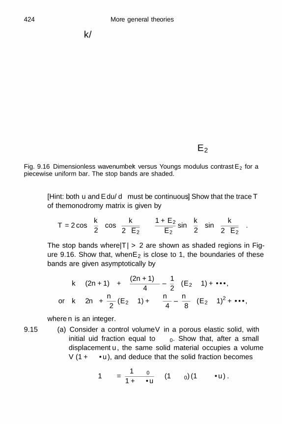
424 More general theories
k/π
E2
Fig. 9.16 Dimensionless wavenumber k versus Young’s modulus contrast E2 for apiecewise uniform bar. The stop bands are shaded.
[Hint: both u and Edu/dξ must be continuous.] Show that the trace T
of themonodromy matrix is given by
T = 2 cos(
k
2
)cos
(k
2√
E2
)− 1 + E2√
E2sin
(k
2
)sin
(k
2√
E2
).
The stop bands where |T | > 2 are shown as shaded regions in Fig-ure 9.16. Show that, when E2 is close to 1, the boundaries of thesebands are given asymptotically by
k ∼ (2n + 1)π +(
(2n + 1)π4
± 12
)(E2 − 1) + · · · ,
or k ∼ 2nπ +nπ
2(E2 − 1) +
(−nπ
4± nπ
8
)(E2 − 1)2 + · · · ,
where n is an integer.9.15 (a) Consider a control volume V in a porous elastic solid, with
initial fluid fraction equal to α0. Show that, after a smalldisplacement u, the same solid material occupies a volumeV (1 + ∇ · u), and deduce that the solid fraction becomes
1 − α =1 − α0
1 + ∇ · u ∼ (1 − α0) (1 − ∇ · u) .

Exercises 425
(b) Now consider a fixed volume V , whose boundary ∂V has unitnormal n, and suppose that fluid with density ρf occupies avolume fraction α. Use the principle ofconservation of massto obtain the equation
ddt
∫∫∫V
ρfα dx = −∫∫
∂Vρfαv · n da,
where v is the average fluid velocity, and deduce that
∂
∂t(ρfα) + ∇ · (ρfαv) = 0.
Show that this reduces to (9.5.7) when the fluid density isconstant and α ≈ α0.

Epilogue
There are three main themes to this book.
1. In Chapters 1–5, we have provided an elementary exposition of the basicconcepts in classical solid mechanics, namely linear elasticity, elastostat-ics, elastodynamics, models for thin structures and nonlinear elasticity.In each case, we have focused on practical examples that highlight themost interesting modelling and mathematical issues.
2. In Chapter 6, our aim was to show how formal perturbation methods,widely used in fluid dynamics, can be applied to many problems in solidmechanics involving bodies that are thin or slender. Although the re-mainder of the book does not rely on this chapter, we firmly believe thatthe techniques demonstrated there form an invaluable component of anyapplied mathematician’s armoury.
3. Finally, in Chapters 7–9, we have given necessarily brief introductionsto some of the important physical situations where classical solid me-chanics fails, and the elementary theories from Chapters 1–5 must bere-examined. Inevitably, the mathematical problems involved here be-come more challenging, and we have therefore limited our attention toidealised models that clearly illustrate the fundamental concepts.
The diversity and open-endedness of the topics described in Chapter 9reflect the fact that we have not done justice to many scientific ideas intheoretical solid mechanics. Fracture, plasticity and viscoelasticity, for ex-ample, are subjects of enormous practical importance, and there are manytexts describing both the practical and the mathematical aspects in muchgreater detail than the contents of Chapters 7–9.
We have not touched at all upon the crucial phase changes that can occurin solids, especially metals and their alloys, as a result of heat treatmentand/or mechanical processing. For example, steel can have several differ-ent crystalline microstructures which can depend crucially on its chemi-cal composition, and these different phases have very different mechanical
426
Epilogue 427
properties. In certain circumstances, the geometry of the phase boundariescan be elegantly described in terms of hyperelasticity, with a strain energydensity possessing multiple minima corresponding to the different phases.This naturally opens up exciting new problems in the calculus of variations,as does the related subject of “shape memory” alloys, where the strain en-ergy depends on temperature. The resulting relaxation phenomena associ-ated with different phases depend on thermal histories in the same way thatviscoelastic relaxation depends on the stress or strain histories.
Another fascinating mathematical challenge that we have not addressed isto find self-contained theories of solids, such as piezoelectric or ferromagneticmaterials, whose mechanical properties depend on electromagnetic fields. Abackground in electromagnetism would be a prerequisite for any appliedmathematician wishing to understand the modelling of such materials.
Finally from the modelling point of view, we must also point out thatwe have avoided any serious discussion of ceramics, which could in factbe defined as any solids that are not metals. Although the mechanics ofmaterials such as rock can be perfectly well described by linear elasticity atsufficiently small stress, little of the theories expounded in Chapters 7 and 8is helpful in understanding how a glass or piece of crockery shatters underimpact, although many ad hoc macroscale models have been proposed.
On the theoretical side, easily our most glaring omission is our failureto discuss the many ingenious numerical schemes that have been specifi-cally developed to solve the kinds of models we have been describing inthis book. Indeed, solid mechanics has provided one of the principal stimulifor the widely-used finite element method, which is so appropriate for find-ing energy minima in complicated real-world configurations of elastic solids.Moreover, computers have now reached the stage where discrete “particle-based” algorithms can be tailored to simulate the mechanics of a solid, beit elastic, plastic or any of the combinations mentioned in this book. At aneven more fundamental level, “atomistic” computations are now routinelyavailable to simulate many, many atoms as points of the solid interacting viasuitable force potentials. Such simulations can give invaluable new insightsinto, say, dislocation interactions and many other nanoscale phenomena.
Despite these qualifications, we hope that this book has shown that a littlesystematic mathematical modelling and analysis can go a long way towardsproviding a firm theoretical formulation for the science of solid mechanics.Even more, we hope that readers will be attracted by the many topics thatawait mathematical attention in an area so important to modern naturalscience.

Appendix
Orthogonal curvilinear coordinates
A1 Framework
Consider a general parametrisation of three-dimensional space, in which theposition vector r of any point is given by
r = r(ξ1, ξ2, ξ3), (A1.1)
in terms of three spatial coordinates ξ1, ξ2 and ξ3. For this to form a sensiblecoordinate system, there should be a one-to-one correspondence between theposition vector r of any point and its coordinates (ξ1, ξ2, ξ3) = ξ. This is thecase provided the Jacobian of the transformation from r to ξ is boundedaway from zero, that is
0 < J < ∞, J = det(
∂r
∂ξ
)=[
∂r
∂ξ1,
∂r
∂ξ2,
∂r
∂ξ3
], (A1.2)
where [·, ·, ·] denotes the triple scalar product between three vectors. By or-dering the coordinates appropriately, we may assume that the tangent vec-tors form a right-handed system and, hence, that J is positive.
A coordinate system is orthogonal if the three tangent vectors created byvarying each of the coordinates in turn are mutually orthogonal, that is
∂r
∂xi· ∂r
∂xj= 0 whenever i = j. (A1.3)
In this case we define the scaling factors hi by
hi =∣∣∣∣ ∂r
∂ξi
∣∣∣∣ , (A1.4)
and the Jacobian is simply given by
J = h1h2h3. (A1.5)
428

A2 Vectors and tensors 429
We can then define a right-handed, mutually orthogonal set of unit vectorse1, e2, e3 by
ei =1hi
∂r
∂ξi(A1.6)
(here the summation convention is not invoked).The most straightforward and familiar coordinate system is Cartesian
coordinates x = (x1, x2, x3), with respect to which the position vector isgiven by r = (x1, x2, x3)
T. This system is clearly orthogonal, with scalefactors all equal to 1.
As another example, consider cylindrical polar coordinates (r, θ, z), withrespect to which r = (r cos θ, r sin θ, z)T. It is straightforward to show thatthis coordinate system is also orthogonal, with scaling factors
hr = 1, hθ = r, hz = 1. (A1.7)
It follows that J = r, so the Jacobian vanishes on the symmetry axis r = 0.This reflects the fact that θ is indeterminate when r = 0 and leads to thepossibility of singular behaviour as r → 0 when solutions of (say) Laplace’sequation are sought in cylindrical polar coordinates.
A2 Vectors and tensors
Consider a vector v with components vi in Cartesian coordinates, that isv = (v1, v2, v3)
T. It is natural to define its components ui in curvilinearcoordinates as ui = v · ei, where ei are the basis vectors defined by (A1.6).If we denote the vector formed by these components by u = (u1, u2, u3)
T,then we have
u =
u1
u2
u3
=
e1 · ve2 · ve3 · v
, (A2.1)
or
u = Pv where P =
eT1
eT2
eT3
. (A2.2)
At each point in space, therefore, our curvilinear coordinate basis is foundby rotating the usual Cartesian basis, the rotation being characterised bythe orthogonal matrix P whose rows are the basis vectors.
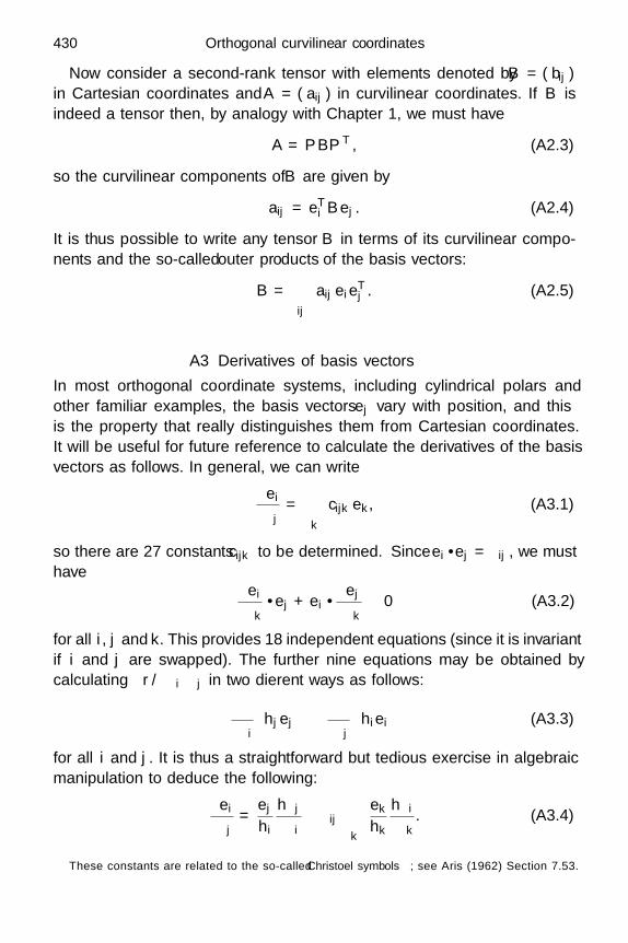
430 Orthogonal curvilinear coordinates
Now consider a second-rank tensor with elements denoted by B = (bij)in Cartesian coordinates and A = (aij) in curvilinear coordinates. If B isindeed a tensor then, by analogy with Chapter 1, we must have
A = PBPT, (A2.3)
so the curvilinear components of B are given by
aij = eTi Bej . (A2.4)
It is thus possible to write any tensor B in terms of its curvilinear compo-nents and the so-called outer products of the basis vectors:
B =∑ij
aijeieTj . (A2.5)
A3 Derivatives of basis vectors
In most orthogonal coordinate systems, including cylindrical polars andother familiar examples, the basis vectors ej vary with position, and thisis the property that really distinguishes them from Cartesian coordinates.It will be useful for future reference to calculate the derivatives of the basisvectors as follows. In general, we can write
∂ei
∂ξj=∑
k
cijkek, (A3.1)
so there are 27 constants cijk to be determined.† Since ei ·ej = δij , we musthave
∂ei
∂ξk· ej + ei ·
∂ej
∂ξk≡ 0 (A3.2)
for all i, j and k. This provides 18 independent equations (since it is invariantif i and j are swapped). The further nine equations may be obtained bycalculating ∂r/∂ξi∂ξj in two different ways as follows:
∂
∂ξi
(hjej
)≡ ∂
∂ξj
(hiei
)(A3.3)
for all i and j. It is thus a straightforward but tedious exercise in algebraicmanipulation to deduce the following:
∂ei
∂ξj=
ej
hi
∂hj
∂ξi− δij
∑k
ek
hk
∂hi
∂ξk. (A3.4)
†These constants are related to the so-called Christoffel symbols; see Aris (1962) Section 7.53.

A4 Scalar and vector fields; grad, div and curl 431
A4 Scalar and vector fields; grad, div and curl
We can think of any scalar field f that varies with position r as being afunction of our coordinate variables: f = f(ξ). Similarly, any vector fieldmay be written as u = u(ξ), and the components of u with respect to thissystem are now written as (u1, u2, u3)
T, where ui = u · ei.The gradient of a scalar field is defined in the usual way in Cartesian
variables, that is
grad f = ∇f =(
∂f
∂x1,
∂f
∂x2,
∂f
∂x3
)T
. (A4.1)
The chain rule leads to
∂f
∂ξi=
∂r
∂ξi· ∇f = hiei · ∇f (A4.2)
and, since the ei are orthonormal, it follows that
∇f =∑
k
1hk
∂f
∂ξkek. (A4.3)
A useful special case occurs if f is one of the variables ξi, when (A4.3) impliesthat
∇ξi =ei
hi. (A4.4)
Now the divergence of a vector field u may be written in terms of Cartesiancoordinates as
div u = ∇ · u =∑
k
∂u
∂xk· ∇xk. (A4.5)
If we rewrite the gradient using (A4.3) and use the chain rule, we find
∇ · u =∑
k
ek
hk· ∂u
∂ξk=∑
k
(1hk
∂uk
∂ξk− u
hk· ∂ek
∂ξk
). (A4.6)
Now we apply (A3.4) to the final term and rearrange to obtain
∇ ·u =1
h1h2h3
∂
∂ξ1
(h2h3u1
)+
∂
∂ξ2
(h1h3u2
)+
∂
∂ξ3
(h1h2u3
). (A4.7)

432 Orthogonal curvilinear coordinates
e1
e2
e3h2δξ2
h1δξ1
h3δξ3
Fig. A1.1 A small reference box B.
Having derived the gradient and divergence, we may now express theLaplacian operator ∇2f = ∇ · (∇f) in terms of arbitrary orthogonal coor-dinates:
∇2f =1
h1h2h3
∂
∂ξ1
(h2h3
h1
∂f
∂ξ1
)+
∂
∂ξ2
(h1h3
h2
∂f
∂ξ2
)+
∂
∂ξ3
(h1h2
h3
∂f
∂ξ3
). (A4.8)
Next, we define the curl of a vector field by
curlu = ∇×u =∑
k
∇xk×∂u
∂xk=∑
k
ek
hk× ∂u
∂ξk. (A4.9)
By rearranging the right-hand side and using (A3.4), this may be trans-formed to
∇×u =∑
k
1hk
∂
∂ξk
(ek×u
)+
u
hk×∂ek
∂ξk=∑i,j
ei×ej
hihj
∂
∂ξi
(hjuj
), (A4.10)
which may be written conveniently as
∇ × u =1
h1h2h3
∣∣∣∣∣∣∣∣∣h1e1 h2e2 h3e3
∂
∂ξ1
∂
∂ξ2
∂
∂ξ3
h1u1 h2u2 h3u3
∣∣∣∣∣∣∣∣∣ . (A4.11)

A4 Scalar and vector fields; grad, div and curl 433
An instructive alternative derivation of (A4.7) may be obtained by apply-ing the divergence theorem to the small box B illustrated in Figure A1.1:∫∫∫
B∇ · u dx =
∫∫∂B
u · n dS =∫∫
[u1h2h3]ξ1 +δξ1ξ1
dξ2dξ3
+∫∫
[u2h1h3]ξ2 +δξ2ξ2
dξ1dξ3 +∫∫
[u3h1h2]ξ3 +δξ3ξ3
dξ1dξ2, (A4.12)
where the integrals on the right-hand side are over the faces ξ1 = const.,ξ2 = const. and ξ3 = const. respectively. In the limit δξ → 0, we thereforeobtain∫∫∫
B(∇ · u)h1h2h3 dξ1dξ2dξ3 ∼
∫∫∫B
∂
∂ξ1(h2h3u1)
+∂
∂ξ2(h1h3u2) +
∂
∂ξ3(h1h2u3)
dξ1dξ1dξ3 (A4.13)
and, since this must hold for all such boxes B, (A4.7) follows.This approach is useful in finding the divergence of a tensor A in curvi-
linear coordinates. By analogy with (A4.5), this is defined in Cartesian co-ordinates to be
div A = ∇ · A =∑
k
∂AT
∂xj∇xk. (A4.14)
By applying the identity∫∫∫B
∇ ·(AT) dx =
∫∫∂B
An dS (A4.15)
to the box B and letting δξ → 0 as above, we find that
∇ ·(AT) =
1h1h2h3
∂
∂ξ1(h2h3Ae1) +
∂
∂ξ2(h1h3Ae2) +
∂
∂ξ3(h1h2Ae3)
.
(A4.16)Now we expand the derivatives and use (A3.4) to obtain
∇ ·(AT) =
∑i,j
ei
J
∂
∂ξj
(aijJ
hi
)+
aij
hi
(ej
hi
∂hj
∂ξi− δij
∑k
ek
hk
∂hi
∂ξk
),
(A4.17)where aij are the curvilinear components of A. Hence we find the ei-component
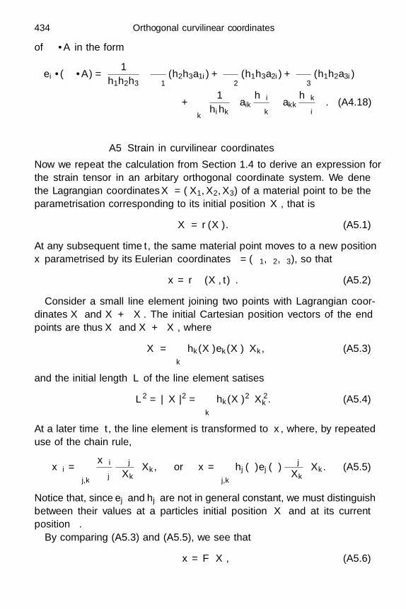
434 Orthogonal curvilinear coordinates
of ∇ · A in the form
ei · (∇ · A) =1
h1h2h3
∂
∂ξ1(h2h3a1i) +
∂
∂ξ2(h1h3a2i) +
∂
∂ξ3(h1h2a3i)
+∑
k
1hihk
(aik
∂hi
∂ξk− akk
∂hk
∂ξi
). (A4.18)
A5 Strain in curvilinear coordinates
Now we repeat the calculation from Section 1.4 to derive an expression forthe strain tensor in an arbitary orthogonal coordinate system. We definethe Lagrangian coordinates X = (X1,X2,X3) of a material point to be theparametrisation corresponding to its initial position X, that is
X = r(X ). (A5.1)
At any subsequent time t, the same material point moves to a new positionx parametrised by its Eulerian coordinates ξ = (ξ1, ξ2, ξ3), so that
x = r(ξ(X , t)
). (A5.2)
Consider a small line element joining two points with Lagrangian coor-dinates X and X + δX . The initial Cartesian position vectors of the endpoints are thus X and X + δX, where
δX =∑
k
hk(X )ek(X )δXk, (A5.3)
and the initial length L of the line element satisfies
L2 = |δX|2 =∑
k
hk(X )2δX 2k . (A5.4)
At a later time t, the line element is transformed to δx, where, by repeateduse of the chain rule,
δxi =∑j,k
∂xi
∂ξj
∂ξj
∂XkδXk, or δx =
∑j,k
hj(ξ)ej(ξ)∂ξj
∂XkδXk. (A5.5)
Notice that, since ej and hj are not in general constant, we must distinguishbetween their values at a particle’s initial position X and at its currentposition ξ.
By comparing (A5.3) and (A5.5), we see that
δx = FδX, (A5.6)
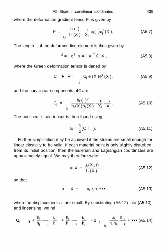
A5 Strain in curvilinear coordinates 435
where the deformation gradient tensor F is given by
F =∑i,j
hi(ξ)hj(X )
∂ξi
∂Xjei(ξ)eT
j (X ). (A5.7)
The length of the deformed line element is thus given by
2 = δxTδx = δXT C δX, (A5.8)
where the Green deformation tensor is defined by
C = FTF =∑i,j
Cijei(X )eTj (X ), (A5.9)
and the curvilinear components of C are
Cij =∑
k
hk(ξ)2
hi(X )hj(X )∂ξk
∂Xi
∂ξk
∂Xj. (A5.10)
The nonlinear strain tensor is then found using
E =12(C − I). (A5.11)
Further simplification may be achieved if the strains are small enough forlinear elasticity to be valid. If each material point is only slightly disturbedfrom its initial position, then the Eulerian and Lagrangian coordinates areapproximately equal. We may therefore write
ξi = Xi +ui(X , t)hi(X )
, (A5.12)
so that
x ∼ X +∑
i
uiei + · · · (A5.13)
when the displacements ui are small. By substituting (A5.12) into (A5.10)and linearising, we find
Cij ∼ δij +hi
hj
∂
∂ξj
(ui
hi
)+
hj
hi
∂
∂ξi
(uj
hj
)+ 2δij
∑k
uk
hjhk
∂hj
∂ξk+ · · · (A5.14)

436 Orthogonal curvilinear coordinates
where it is no longer necessary to distinguish between ξ and X within thelinear theory. The linearised strain components in curvilinear coordinatestherefore read
eij =12
1hj
∂ui
∂ξj− ui
hihj
∂hi
∂ξj+
1hi
∂uj
∂ξi− uj
hihj
∂hj
∂ξi
+ δij
∑k
uk
hjhk
∂hj
∂ξk.
(A5.15)
A6 Stress in curvilinear coordinates
As in Section 1.5, we define the Cauchy stress τij to be the component in theei-direction of the stress acting on a surface element whose normal pointsalong ej . Although the basis vectors ei may now vary with position, at anyfixed location, the curvilinear components τij of the stress tensor are foundby simply rotating the Cartesian components through the orthogonal matrixP introduced in Section A2. It is easily shown that the symmetry of τij inCartesian coordinates is maintained in an arbitrary orthogonal coordinatesystem.
In Section 1.7, we introduced the constitutive relation
τij = λ (ekk) δij + 2µeij , (A6.1)
which links the stress and linearised strain tensors in a linear elastic material.Note that, since τij and eij are tensors, they both obey the transformationrule (A2.3) if the coordinate axes are rotated by an orthogonal matrix P ,which may be a function of position. Hence, although the relation (A6.1)was originally posed using fixed Cartesian coordinates, it actually holds inany orthogonal coordinate system.
A7 Examples of orthogonal coordinate systems
A7.1 Cylindrical polar coordinates
The Cartesian position vector is given in terms of the coordinate variables(r, θ, z) by r = (r cos θ, r sin θ, z)T, as illustrated in Figure A1.2. The scalingfactors are given by (A1.7), and therefore the formulae for the gradient,

A7 Examples of orthogonal coordinate systems 437
r
θ
z
z
y
x
Fig. A1.2 Cylindrical polar coordinates.
divergence, Laplacian and curl in this coordinate system are
∇f =∂f
∂rer +
1r
∂f
∂θeθ +
∂f
∂zez , (A7.1a)
∇ · u =1r
∂
∂r(rur) +
1r
∂uθ
∂θ+
∂uz
∂z, (A7.1b)
∇2f =1r
∂
∂r
(r∂f
∂r
)+
1r2
∂2f
∂θ2 +∂2f
∂z2 , (A7.1c)
∇×u =(
1r
∂uz
∂θ− ∂uθ
∂z
)er +
(∂ur
∂z− ∂uz
∂r
)eθ +
1r
(∂
∂r(ruθ) −
∂ur
∂θ
)ez ,
(A7.1d)
where f is any scalar field and u = urer + uθeθ + uzez is any vector field(both suitably differentiable). The components of the linearised strain tensorcorresponding to a displacement field u are given by
err =∂ur
∂r, 2erθ =
1r
∂ur
∂θ+
∂uθ
∂r− uθ
r, (A7.2a)
eθθ =1r
(∂uθ
∂θ+ ur
), 2erz =
∂ur
∂z+
∂uz
∂r, (A7.2b)
ezz =∂uz
∂z, 2eθz =
∂uθ
∂z+
1r
∂uz
∂θ. (A7.2c)
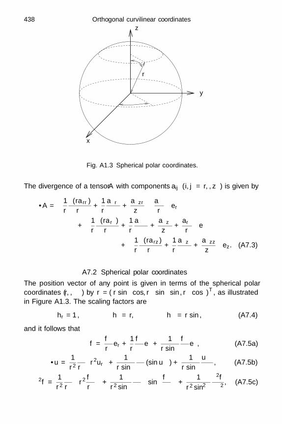
438 Orthogonal curvilinear coordinates
r
φ
θ
z
y
x
Fig. A1.3 Spherical polar coordinates.
The divergence of a tensor A with components aij (i, j = r, θ, z) is given by
∇ · A =
1r
∂(rarr)∂r
+1r
∂aθr
∂θ+
∂azr
∂z− aθθ
r
er
+
1r
∂(rarθ)∂r
+1r
∂aθθ
∂θ+
∂azθ
∂z+
aθr
r
eθ
+
1r
∂(rarz)∂r
+1r
∂aθz
∂θ+
∂azz
∂z
ez . (A7.3)
A7.2 Spherical polar coordinates
The position vector of any point is given in terms of the spherical polarcoordinates (r, θ, φ) by r = (r sin θ cos φ, r sin θ sinφ, r cos θ)T, as illustratedin Figure A1.3. The scaling factors are
hr = 1, hθ = r, hφ = r sin θ, (A7.4)
and it follows that
∇f =∂f
∂rer +
1r
∂f
∂θeθ +
1r sin θ
∂f
∂φeφ, (A7.5a)
∇ · u =1r2
∂
∂r
(r2ur
)+
1r sin θ
∂
∂θ(sin θuθ) +
1r sin θ
∂uφ
∂φ, (A7.5b)
∇2f =1r2
∂
∂r
(r2 ∂f
∂r
)+
1r2 sin θ
∂
∂θ
(sin θ
∂f
∂θ
)+
1r2 sin2 θ
∂2f
∂φ2 , (A7.5c)
A7 Examples of orthogonal coordinate systems 439
∇×u =1
r sin θ
(∂
∂θ(sin θuφ) − ∂uθ
∂φ
)er
+(
1r sin θ
∂ur
∂φ− ∂uφ
∂r
)eθ +
1r
(∂
∂r(ruθ) −
∂ur
∂θ
)eφ, (A7.5d)
for any suitably differentiable f and u = urer+uθeθ+uφeφ. The componentsof the linear strain tensor in spherical polars read
err =∂ur
∂r, (A7.6a)
2erθ =1r
∂ur
∂θ+
∂uθ
∂r− uθ
r, (A7.6b)
eθθ =1r
(∂uθ
∂θ+ ur
), (A7.6c)
2erφ =1
r sin θ
∂ur
∂φ+
∂uφ
∂r− uφ
r, (A7.6d)
eφφ =1
r sin θ
∂uφ
∂φ+
ur
r+
cot θuθ
r, (A7.6e)
2eθφ =1
r sin θ
∂uθ
∂φ+
1r
∂uφ
∂θ− cot θuφ
r, (A7.6f)
and the divergence of a tensor A is given by
∇ · A =
1r2
∂(r2arr)∂r
+1
r sin θ
∂(sin θaθr)∂θ
+1
r sin θ
∂aφr
∂φ− aθθ + aφφ
r
er
+
1r2
∂(r2arθ)∂r
+1
r sin θ
∂(sin θaθθ)∂θ
+1
r sin θ
∂aφθ
∂φ+
aθr − cot θaφφ
r
eθ
+
1r2
∂(r2arφ)∂r
+1
r sin θ
∂(sin θaθφ)∂θ
+1
r sin θ
∂aφφ
∂φ+
aφr + cot θaφθ
r
eφ.
(A7.7)

References
Abramowitz, M. & Stegun, I. A. 1972 Handbook of Mathematical Functions(tenth printing). Dover.
Aris, R. 1962 Vectors, Tensors, and the Basic Equations of Fluid Mechanics.Dover.
Barber, J. R. 1993 Elasticity. Springer.Batchelor, G. K. 2000 An Introduction to Fluid Dynamics (New Edition).
Cambridge University Press.Bender, C. M. & Orszag, S. A. 1978 Advanced Mathematical Methods for Sci-
entists and Engineers. McGraw–Hill.Bland, D. R. 1988 Wave Theory and Applications. Clarendon Press.Bleistein, N. 1984 Mathematical Methods for Wave Phenomena. Academic Press.Boyce, W. E. & DiPrima, R. C. 2004 Elementary Differential Equations and
Boundary Value Problems (Eighth Edition). Wiley.Brillouin, L. 2003 Wave Propagation in Periodic Structures. Dover.Calladine C. R. 2000 Plasticity for Engineers: Theory and Applications. Horwood
Publishing Ltd.Carrier, G. F., Krook, M. & Pearson, C. E. 1983 Functions of a Complex
Variable: Theory and Technique. Hod Books.Drazin, P. G. & Johnson, R. S. 1989 Solitons: an Introduction. Cambridge
University Press.Elliott, C. M. & Ockendon, J. R. 1982 Weak and Variational Methods for
Free and Moving Boundary Problems. Pittman.England, A. H. 2003 Complex Variable Methods in Elasticity. Dover.Fowler, A. C. 1997 Mathematical Models in the Applied Sciences. Cambridge
University Press.Freund, L. B. 1989 Dynamic Fracture Mechanics. Cambridge University Press.Fung, Y. C. & Tong, P. 2001 Classical and Computational Solid Mechanics.
World Scientific.Gradshteyn, I. S. & Ryzhik, I. M. 1994 Table of Integrals, Series, and Products
(Fifth Edition). Academic Press.Hill, R. 1998 The Mathematical Theory of Plasticity. Oxford University Press.Hinch, E. J. 1991 Perturbation Methods. Cambridge University Press.Hirth, J. P. & Lothe, J. 1991 Theory of Dislocations. Krieger Publishing
Company.Hooke, R. 1678 De Potentia Restitutiva or of Spring Explaining the Power of
440

References 441
Springing Bodies. John Martyn at The Bell in St Paul’s Churchyard.Howison, S. D. 2005 Practical Applied Mathematics: Modelling, Analysis,
Approximation. Cambridge University Press.Jordan, D. W. & Smith, P. 1999 Nonlinear Ordinary Differential Equations: an
Introduction to Dynamical Systems. Oxford University Press.Kac, M. 1966 Can one hear the shape of a drum? Am. Math. Monthly 73, 1–23.Keener, J. P. 2000 Principles of Applied Mathematics, Transformation and
Approximation (Revised Edition). Westview Press.Kevorkian, J. & Cole, J. D. 1981 Perturbation Methods in Applied Mathemat-
ics. Springer-Verlag.Kreyszig, E. 1959 Differential Geometry. Dover.Lakes, R. 1987 Foam structures with a negative Poisson’s ratio. Science 235,
1038–1040.Love, A. E. H. 1944 A Treatise on the Mathematical Theory of Elasticity. Dover.Mindlin, R. D. 1939 Stress distribution around a tunnel. Proc. ASCE 65, 619.Noll, W. 1958 A mathematical theory of the mechanical behaviour of continuous
media. Arch. Rational Mech. Anal. 2, 197–226.Ockendon, H. & Ockendon, J. R. 1995 Viscous Flow. Cambridge University
Press.Ockendon, J. R., Howison, S. D., Lacey, A. A. & Movchan, A. B. 2003
Applied Partial Differential Equations (Revised Edition). Oxford UniversityPress.
Priestley, H. A. 2003 Introduction to Complex Analysis. Oxford University Press.Salazar, D. & Westbrook, R. 2004 Inverse problems of mixed type in linear
plate theory. Euro. J. Appl. Math. 15, 129–146.Sneddon, I. N. & Lowengrub, M. 1970 Crack Problems in the Classical Theory
of Elasticity. Wiley.Spencer, A. J. M. 1970 The static theory of finite elasticity. J. Inst. Maths
Applics. 6, 164–200.Strang, G. 1988 Linear Algebra and its Applications (Third Edition). Harcourt
Brace Jovanovich College Publishers.Tayler, A. B. 2002 Mathematical Models in Applied Mechanics (New Edition).
Oxford University Press.Thomas, T. Y. 1961 Plastic Flow and Fracture in Solids. Academic Press.Timoshenko, S. P. & Goodier, J. N. 1970 Theory of Elasticity. McGraw–Hill.Timoshenko, S. P. & Woinowsky-Krieger, S. 1959 Theory of Plates and
Shells. McGraw–Hill.Treloar, L. R. G. 2005 The Physics of Rubber Elasticity. Oxford University
Press.Vaziri, A. & Mahadevan, L. 2008 Localized and extended deformations of elastic
shells. PNAS 105(23), 7913–7918.Weertman, J. & Weertman, J. R. 1992 Elementary Dislocation Theory (New
Edition). Oxford University Press.

Index
aerofoil, 293, 344airliner, 287Airy function, 212Airy stress function, 47–68, 71, 82, 171, 176,
179, 252, 264, 297, 304, 307, 323, 334,341, 350, 374
boundary conditions, 49–51, 297modified, 66, 86, 98plane stress, 74polar coordinates, 51uniqueness, 48, 50
Airy’s equation, 212alloy, 426
shape memory, 427alternating symbol, 82, 100analytic continuation, 296, 299angle of friction, 330, 336, 372angle of incidence, 116, 145angle of reflection, 116, 145angle of repose, 330angular momentum, 9, 25, 154, 197, 268, 274angular velocity, 196, 197anisotropy, 379, 398, 404, 410, 413–417annulus
plane strain in, 53–56torsion in, 44
anticlastic shell, 181, 184anticlastic surface, 179antiplane strain, 37–39, 80, 246–248, 258, 283,
338, 395dynamic, 117, 135, 308, 324in a strip, 247yield criterion, 345
antiplane stress function, 41, 82, 97, 339, 345uniqueness, 41
associated flow rule, 362asymptotic expansion, 194, 245, 247, 257, 275,
394, 397, 403, 407atomistic model, 1, 337–344, 427auxetic material, 33, 55, 93axe, 289
balloon, 235, 244
bar, 104, 150–152, 242boundary conditions, 152, 189composite, 392–395, 404–408constitutive relation, 152multiply-conected, 42thermoelastic, 389, 421torsion, 39, 42, 93viscoelastic, 385
basis vectors, 27, 279, 429, 430Bauschinger effect, 374beam, 150
bending, 76boundary conditions, 156compression, 156, 158, 191–195constitutive relation, 154, 189contact, 313, 325linear, 153–158, 205, 206, 213nonlinear, 187–195, 197, 210, 211unsteady, 200–204
beam equationEuler–Bernoulli, 189linear, 155nonlinear, 189
bending, 76, 174, 183, 196, 198bending moment, 61, 62, 154, 159, 163–165,
189, 251, 252, 263, 266, 271, 275, 277bending stiffness, 150, 154, 158, 160, 165, 170,
208, 281, 313Bessel function, 108, 109, 113, 124, 131Bessel’s equation, 107, 109, 126
inhomogeneous, 127biaxial strain, 33–35, 76, 171, 234bicycle frame, 46bifurcation, 195, 235biharmonic equation, 48, 56, 71, 74, 168, 171,
253, 296, 304, 350axisymmetric, 77boundary conditions, 96inhomogeneous, 66, 77, 78, 168, 341polar coordinates, 51
biomaterial, 14, 379body force, 10, 219
conservative, 65
442

Index 443
in plane strain, 65–68boundary conditions, 16–18
Airy stress function, 49–51, 297between two solids, 18, 118Cauchy, 18clamped, 156, 166, 168, 189, 191Dirichlet, 16, 39, 41, 44, 181elliptic, 18free, 156, 166mixed, 18, 296, 317natural, 26, 39, 167, 168, 209Neumann, 17, 39, 40, 259, 276, 290on a bar, 152, 189on a beam, 156on a plate, 166–168, 171, 176, 208, 253–261on a rod, 160periodic, 397, 422point force, 87pressure, 51Robin, 27simply supported, 156, 166, 168, 170, 189,
208stress-free, 31, 33, 40, 50, 54, 66, 86, 121,
124, 125, 128, 130, 131, 248, 250, 263,274, 290
traction, 17, 26, 38, 49, 56, 58, 62, 66, 156,254
boundary element method, 90boundary layer, 46, 167, 182, 247, 253–261branch cut, 292, 338Brillouin zone, 408brittle fracture, 288, 344buckling, 2, 157, 191–195, 205, 212, 213, 390bulk modulus, 30Burgers vector, 342
cable, 198calculus of variations, 26, 39, 51, 168, 176,
209, 210, 229, 239, 427capstan, 321car
panel, 150suspension, 39, 380tyre, 13, 287
Cartesian coordinates, 19–20, 429cartilage, 13catenary, 210Cauchy data, 18Cauchy stress tensor, 9, 218, 219, 225, 229,
232, 242, 280Cauchy’s momentum equation, 10, 219, 250,
255, 273, 334, 360, 386Cartesian coordinates, 20cylindrical polar coordinates, 21Lagrangian form, 220, 263, 268plane polar coordinates, 335spherical polar coordinates, 23, 238
Cauchy–Riemann equations, 339, 400causality, 141cavitation, 237, 289cavity, 91, 237, 243
Cayley–Hamilton theorem, 223centroid, 274ceramic, 379, 427characteristic, 137, 148, 210, 221, 282, 334, 350characteristic cone, 137, 148characteristic polynomial, 222, 223Christoffel symbols, 430coal, 117, 146, 330coarse-graining, 391coefficient
of friction, 320of reflection, 112, 116, 144, 145of restitution, 321of thermal expansion, 389of transmission, 112, 144
cohesion, 294, 322, 337compatibility, 54, 68–70, 82, 97, 100, 174, 339,
348in terms of stress, 72, 100, 101plane strain, 69, 101three-dimensional, 69
complementarity conditions, 312, 349, 365completeness, 61complex eigenvalues, 60complex modulus, 419composite, 378, 391–408compressibility, 410cone, 175
characteristic, 137, 148Mach, 141, 143two-sheeted, 137, 143
conformal transformation, 291, 295, 298, 322,323, 325
conjugate function, 298conservative body force, 65constitutive relation, 3, 11
Cartesian coordinates, 19cylindrical polar coordinates, 20elastic-plastic, 365, 366for a bar, 152for a beam, 154, 189, 271for a plate, 164, 171, 271for a rod, 160, 161, 196, 276for a shell, 281homoclinic, 414incompressible, 232isotropic, 12, 225, 241, 402Jeffreys, 417, 419linear, 12, 32, 68, 231, 256, 265, 270, 275,
402, 413Maxwell, 382, 383, 385, 419Mooney–Rivlin, 232, 234, 236, 387neo-Hookean, 232, 238, 387nonlinear, 221–233objective, 224, 228Ogden, 232one-dimensional, 220orthotropic, 414spherical polar coordinates, 22thermoelastic, 389transversely isotropic, 415

444 Index
Varga, 232Voigt, 381, 383–385, 418
contact, 287, 309–320bonded, 18frictional, 18, 320of a beam, 313, 325of a membrane, 316, 326of a plate, 317of a string, 309–313plane strain, 317–320smooth, 18
contact set, 287, 309continuum, 3convected derivative
corotational, 388, 420Jaumann, 388, 420lower, 387upper, 387
convective derivative, 358, 376, 387, 388, 419convolution, 63, 96coordinates
Cartesian, 19–20, 429curvilinear, 278, 428–439cylindrical polar, 20–22, 365, 429, 436–438elliptic, 291Eulerian, 3, 11, 172, 216, 267, 376, 434Lagrangian, 3, 11, 172, 188, 196, 216, 218,
219, 267, 376, 434orthogonal, 19, 278, 428spherical polar, 22–24, 235, 237, 438–439
copper, 13corotational derivative, 388, 420Coulomb friction, 320, 330, 332Coulomb yield criterion, 333, 335, 353, 357,
372Coulomb yield surface, 358crack, 287–309
elliptical, 291, 297, 304, 321Griffith, 289Mode I, 304–307, 323, 344Mode II, 296–304, 344Mode III, 290–295, 308, 321, 322, 324, 344penny-shaped, 307
crack face, 288crack tip, 287, 288, 290, 321, 344crease, 182, 187creep, 383creep function, 383, 386curl
curvilinear coordinates, 432cylindrical polar coordinates, 437spherical polar coordinates, 439tensor, 70, 82, 100
curl curl, 13curtain rod, 150curvature, 154, 165, 166, 189, 236, 271, 315
Gaussian, 168, 170, 174, 176, 178, 181, 282lines of, 278mean, 168principal, 168, 174, 279radius of, 188, 293, 321
curvature tensor, 281curvilinear coordinates, 278, 428–439custard, 378cut-and-weld operation, 338, 340cut-off frequency, 120, 125cylinder, 175, 178, 183, 281
waves in, 124–128cylindrical polar coordinates, 20–22, 365, 429,
436–438
d’Alembert solution, 132, 148damped solid, 382Darcy’s law, 409dashpot, 380Deborah number, 379, 382deformable porous medium, 408deformation gradient, 216, 221, 224, 264, 270,
377, 419del squared, 13delta-function, 82–84, 88, 133, 139, 149, 167,
206, 315, 339, 421derivative of, 92multidimensional, 83
densityline, 18, 24, 152reference, 4, 219surface, 104, 162volume, 4, 11, 219, 376
determinant, 119, 126, 128, 146developable shell, 181, 183, 188developable surface, 174, 178deviatoric stress, 354, 363, 369, 375, 386diamond, 13diffusion coefficient, 410diffusion equation, 410dilatational viscosity, 384directivity function, 113Dirichlet problem, 16, 39, 41, 44, 181disc
plane strain in, 51–53dislocation, 337–344
edge, 342mixed, 342screw, 342, 373virtual, 295, 344
dispersion relation, 110anisotropic, 417for a beam, 158of Love waves, 120, 145
dispersive wave, 111, 119displacement, 1, 3, 358
linear, 29–37single-valued, 44, 54, 67, 98, 99virtual, 26, 176, 209, 232, 313
displacement gradient, 35, 100, 359dissipation, 2, 361, 364, 419
maximal, 362distinguished limit, 202, 262distribution, 83divergence, 10
curvilinear coordinates, 431, 434

Index 445
cylindrical polar coordinates, 21, 437, 438spherical polar coordinates, 24, 438, 439
diving board, 187, 190–191, 211diving cylinder, 53door slamming, 380drag, 379, 409drill, 289drum, 107, 150ductile fracture, 289Duffing equation, 194dynamic antiplane strain, 117, 135, 308, 324dynamic fracture, 308, 324dynamic Love function, 122, 123, 125, 142dynamic plane strain, 122, 142, 147
in a half-space, 120
earthquake, 114, 121, 308edge dislocation, 342eigenfunctions, 61, 96, 107, 157eigenvalue problem
nonlinear, 192not self-adjoint, 60
eigenvalues, 35, 36, 96, 107, 157, 221, 406complex, 60
eigenvectors, 35, 222, 225eikonal equation, 331, 348elastic energy, 15, 39, 226, 229, 377, 390elastic fluid, 383elastic modulus, 3, 32, 413
effective, 399, 401, 404, 409, 423elastic strain, 364, 377, 384electromagnetic wave, 104, 137, 404electromagnetism, 427electron micrograph, 343elliptic boundary conditions, 18elliptic coordinates, 291elliptic integral, 191, 213energy
bending, 316conservation of, 14–16, 24, 226–227,
360–362, 391elastic, 15, 39, 226, 229, 377, 390kinetic, 15, 226, 360, 390surface, 289thermal, 360, 390
energy equation, 361, 391, 420envelope, 137, 148equivoluminal wave, 114, 122Euler differential equation, 52Euler strut, 192, 210, 212Euler’s identity, 376Euler–Bernoulli beam equation, 189Euler–Lagrange equation, 316Eulerian coordinates, 3, 11, 172, 216, 267, 376,
434
fabric, 379ferromagnetism, 427fibre-reinforced material, 12, 379, 413Finger tensor, 217, 223, 225, 387, 419finite element method, 229, 427
first fundamental form, 278first law of thermodynamics, 361, 390flexural wave, 126, 128, 283Floquet theory, 405flow rule, 362–364
associated, 362Levy–von Mises, 363, 377non-associated, 362Tresca, 363, 366
fluidelastic, 383inviscid, 7, 82, 340, 343, 371lower convected Maxwell, 387Maxwell, 386Newtonian, 364, 386upper convected Maxwell, 387viscous, 379, 380, 408with memory, 383
fluid fraction, 410, 424food, 330, 378force balance, 17, 39, 53, 56, 188, 309, 313, 330Fourier series, 57, 106, 248Fourier transform, 62, 87, 96, 101, 106, 111,
115, 213, 296three-dimensional, 99
Fourier’s law of conduction, 391fracture, 2, 287–309, 426
brittle, 288, 344ductile, 289dynamic, 308, 324
frame indifference, 224, 228Fredholm Alternative, 17free boundary problem, 287, 310, 334, 349,
350, 365frequency, 110
cut-off, 120, 125frequency domain, 105, 404friction, 320
angle of, 330, 336, 372coefficient of, 320Coulomb, 320, 330, 332
Frobenius’ method, 108, 131fundamental form
first, 278second, 278
fundamental solution, 82, 133–136one-dimensional, 133three-dimensional, 136two-dimensional, 135
Galerkin representation, 78–79garden hose, 198gauge invariance
Airy stress function, 48, 50antiplane stress function, 41Love function, 74Papkovich–Neuber potentials, 81
Gaussian curvature, 168, 170, 174, 176, 178,181, 282
generalised function, 83generator, 175, 178, 183, 188, 282

446 Index
geometric nonlinearity, 11, 151, 172, 174, 188,215, 231, 262, 282, 386
glass, 13, 150, 169, 353, 378, 391Goursat representation, 49, 80, 95, 297, 304,
323, 324grad div, 13gradient
curvilinear coordinates, 431cylindrical polar coordinates, 437spherical polar coordinates, 438
granite, 13granular plasticity, 330–337Green deformation tensor, 216, 222, 361, 419,
435left, 217
Green’s function, 88, 140Green’s tensor, 88–90
plane strain, 89three-dimensional, 99
Griffith crack, 289group velocity, 146guitar, 153gun barrel, 37, 53, 91, 335, 351
elastic-plastic, 366–368failure, 55
gyroscope, 198
hair, 150, 213half-space
dynamic plane strain in, 120plane strain in, 62–65, 86, 317–320
Hankel function, 113harmonic average, 393harmonic conjugate, 41, 45, 303, 339, 400, 422harmonic wave, 110, 113harmonics, 105, 158
out of tune, 109heat equation, 391, 411heat flux, 391Heaviside function, 134, 207, 373, 421Helmholtz equation, 107
plane polar coordinates, 109, 144radially symmetric, 107two-dimensional, 112
Helmholtz representation, 71, 78Hilbert transform, 64, 97
inverse, 97history-dependence, 329homoclinic material, 414homogenisation, 379, 391–408, 410, 422–424
three-dimensional, 402–404two-dimensional, 395–402
Hooke’s law, 2, 12, 152, 380hoop stress, 55, 68, 99Hopkinson bar test, 207Huygens’ principle, 136hydrostatic stress, 30, 99hyperboloid, 175hyperelasticity, 215, 227–230, 361, 427
I-beam, 161
ice cube, 388ice sheet, 138impedance, 380, 417in-plane strain, 34, 171incidence
angle of, 116, 145incident wave, 112, 115, 207incompatibility, 70, 72
line, 339, 341point, 91–92tensor, 92, 343
incompressibility, 13, 26, 33, 143, 231–232,343, 359, 363, 386
inertia, 333, 346, 350, 365, 371, 410inertia tensor, 160, 197, 278inextensibility, 188, 196, 205, 269, 272initial-value problem, 132instability, 158, 195, 211integral equation, 90, 296, 322inverse problem, 143, 169–170, 208inverse scattering, 113, 199irreversibility, 2, 328, 362irrotational wave, 114, 122isometry, 174, 178isotropic expansion, 29, 30, 389, 420isotropic invariant, 222isotropy, 12, 224, 228, 230, 241, 353
Jacobian, 4, 11, 218, 231, 376, 428Jaumann derivative, 388, 420Jeffreys constitutive relation, 417, 419Jeffreys creep function, 418Jeffreys element, 417, 419
KdV equation, 204, 214kinetic energy, 15, 226, 360, 390kink, 200Kirchhoff analogy, 198knot, 321Kronecker delta, 12
Luders bands, 368–370ladder, 320Lagrange multiplier, 26, 95, 231, 362Lagrangian coordinates, 3, 11, 172, 188, 196,
216, 218, 219, 267, 376, 434Lame constants, 12, 13, 29, 32, 230, 338, 384,
389, 409Lame equation, 13Laplace’s equation, 38, 79, 93, 258, 276, 290,
399, 416general solution, 48, 94
Laplaciancurvilinear coordinates, 432cylindrical polar coordinates, 21, 437spherical polar coordinates, 24, 438two-dimensional, 104
lawn-mower, 214left Green deformation tensor, 217Legendre polynomial, 131Levi–Civita symbol, 82, 100

Index 447
Levy–von Mises flow rule, 363, 377line density, 18, 24, 152linear displacement, 29–37linear elasticity, 11–13, 230lines of curvature, 278Liouville’s theorem, 299longitudinal wave, 114, 115, 125, 151, 207,
221, 283loss modulus, 419Love function, 82
axisymmetric, 76–78, 100dynamic, 122, 123, 125, 142plane strain, 73–74, 78, 84, 86uniqueness, 74
Love wave, 117–120, 145, 417lower convected derivative, 387lower convected Maxwell fluid, 387
Mach cone, 141, 143Mach number, 140, 142, 201mass
conservation of, 4, 359, 376, 410, 425matching condition, 61, 248, 256material symmetry, 413matrix
monodromy, 406, 424orthogonal, 6, 9, 12, 35, 37, 216, 217, 221,
223, 224, 240, 241, 413positive definite, 221, 413
maximal dissipation, 362maximum shear stress, 37, 55, 85, 95, 301,
306, 354Maxwell constitutive relation, 382, 383, 385,
419Maxwell creep function, 383, 418Maxwell element, 382, 383Maxwell fluid, 386Maxwell stress functions, 81–82Maxwell’s equations, 137mean curvature, 168mechanical linearity, 174, 188, 215, 220, 231,
265, 270membrane, 39, 93, 104, 135, 140, 150, 165,
234, 235, 262contact, 316, 326
metal plasticity, 337–370method of images, 86method of multiple scales, 393, 396, 403, 407,
423Miura transform, 214mixed dislocation, 342mode conversion, 103, 115–117Mode I crack, 304–307, 323, 344Mode II crack, 296–304, 344Mode III crack, 290–295, 308, 321, 322, 324,
344modified KdV equation, 204, 214modulus of compression, 30Mohr circle, 333, 350Mohr surface, 373
moment balance, 9, 17, 26, 56, 154, 159, 162,163, 188, 198, 313
moment of inertia, 154, 155momentum
conservation of, 10–11, 219–220, 360momentum equation, 10, 219, 250, 255, 273,
334, 360, 386Cartesian coordinates, 20cylindrical polar coordinates, 21Lagrangian form, 220, 263, 268plane polar coordinates, 335spherical polar coordinates, 23, 238
Monge–Ampere equation, 174, 209, 334, 350inhomogeneous, 178
monodromy matrix, 406, 424Mooney–Rivlin constitutive relation, 232, 234,
236, 387Morera stress functions, 81–82moving source, 138–143, 149multi-scaling, 391multiple scales
method of, 393, 396, 403, 407, 423multiply-connected domains, 42–47, 53–56, 67musical instruments, 105
natural boundary conditions, 26, 39, 167, 168,209
natural frequenciesof a drum, 108of a membrane, 107, 143of a piano string, 205of a sphere, 130of a string, 105
Navier equation, 13, 137anisotropic, 416axisymmetric, 76Cartesian coordinates, 20cylindrical polar coordinates, 21general solution, 115incompressible, 26poroelastic, 409spherical polar coordinates, 23steady, 16, 29steady plane strain, 47thermoelastic, 389unsteady, 113
neo-Hookean constitutive relation, 232, 238,387
Neumann problem, 17, 39, 40, 259, 276, 290Newton’s second law, 8, 10, 151, 153, 158, 162,
219Newton’s third law, 7non-associated flow rule, 362non-contact set, 309non-destructive testing, 143non-dimensionalisation, 180, 193, 202, 246,
249, 262, 267, 273, 279, 393, 404, 421non-dispersive wave, 111nonlinear beam equation, 189nonlinear wave, 198–204, 220–221normal modes, 104–109

448 Index
of a membrane, 107of a string, 105superposition, 106
normal reaction, 330normal stress, 37, 332, 372nucleus of strain, 92, 102
objectivity, 217, 224, 228, 388obstacle, 309Ogden constitutive relation, 232oil reservoir, 408orthogonal coordinates, 19, 278, 428orthogonal matrix, 6, 9, 12, 35, 37, 216, 217,
221, 223, 224, 240, 241, 413orthotropic material, 414outer product, 430
π-plane, 355P -wave, 103, 114, 221, 417
reflection, 115Peclet number, 412pantograph, 138paper, 150, 160, 165, 174, 183paper clip, 2, 198, 328, 359, 360, 371paper model, 33, 93Papkovich–Neuber potentials, 79–81, 87, 296,
301, 305, 340, 344, 373antiplane strain, 80plane strain, 80, 100uniquness, 81
partial differential equationchange of type, 153, 170, 334, 349completely integrable, 199discriminant, 170, 181elliptic, 16, 140, 143, 155, 179, 181, 282, 334,
399hyperbolic, 137, 140, 155, 170, 179, 181,
282, 334, 346, 350, 372mixed type, 143, 170parabolic, 178, 282quasi-linear, 209
pass band, 406pendulum, 190, 198penny-shaped crack, 307perfect plasticity, 328, 331, 334, 344–357periodic cell, 393, 397, 403, 422permanent strain, 328, 348, 374, 385permeability, 409phase change, 426phase velocity, 110piano, 109, 158, 205piezoelectricity, 427ping-pong ball, 150, 186Piola–Kirchhoff stress tensor, 218–219
first, 219, 227, 263, 264, 268second, 219, 224, 225, 228, 242, 265
pitchfork bifurcation, 195plane polar coordinates, 27plane strain, 35, 47–68, 71–74, 80, 84, 99, 165,
171, 296, 297, 304, 340, 375contact, 317–320
dynamic, 120, 122, 142, 147elastic-plastic, 350–353in a disc, 51–53in a half-space, 62–65, 86, 317–320in a rectangle, 56–58in a strip, 58–62in an annulus, 53–56with a body force, 65–68yield criterion, 350, 376
plane stress, 74–76, 99, 155, 159, 163, 368plane wave, 110–111, 137plastic bottle, 184plastic flow, 2plastic strain, 364, 370plastic yield, 37, 85, 294plasticity, 289, 328–377, 379, 426
granular, 330–337metal, 337–370perfect, 328, 331, 334, 344–357
plate, 33–35, 150, 368antiplane strain in, 246–248, 283boundary conditions, 166–168, 171, 176,
208, 253–261circular, 168, 208constitutive relation, 164, 171, 271contact, 317linear, 162–171, 248–253nonlinear, 267–273rectangular, 169strain energy density, 168, 176, 209strain in, 173von Karman, 172–176, 261–267
plate equationlinear, 165, 171, 253von Karman, 176, 267
point forcein a half-space, 86on a half-space, 87plane strain, 84, 101three-dimensional, 85, 100
point incompatibility, 91–92Poisson’s equation, 41, 79, 140, 316, 345
singular solutions, 84Poisson’s ratio, 32, 165, 384, 390
negative, 33, 55, 93polar decomposition, 221, 241polarised wave, 114polystyrene, 13pore pressure, 409poroelasticity, 2, 379, 408–412, 424–425positive definite matrix, 221, 413Prandtl–Reuss model, 370pre-stressed material, 12pressure, 14, 30, 231, 354, 375, 386
hydrostatic, 232pore, 409
pressure wave, 114primary wave, 114principal axes, 35, 36, 160, 197principal curvature, 168, 174, 279principal direction, 35, 175, 222

Index 449
principal strain, 35, 222, 230principal stress, 36, 55, 85, 95, 229, 234, 242,
332, 354, 363, 372principal stretch, 222, 230principal value integral, 64, 97, 322punch, 317
quadratic form, 5quantum mechanics, 130quasi-static problem, 93
radiation condition, 112radius of curvature, 293, 321railway
track, 378, 390underground, 66
rate-of-strain tensor, 359, 363, 377, 386Rayleigh wave, 120–121, 146razor blade, 214reaction force, 206, 312, 315, 317rectangle
plane strain in, 56–58reference density, 4, 219reference state, 1, 3, 215, 216, 222, 389reflected wave, 116, 207reflection
angle of, 116, 145of a P -wave, 115of an S -wave, 144specular, 116total internal, 117, 145
reflection coefficient, 112, 116, 144, 145region of influence, 179, 334relaxation time, 381, 382, 384, 417residual stress, 12, 348, 352response diagram, 192, 195, 212, 213, 235retarded potential, 136Reynolds’ transport theorem, 376rheological test, 419Riemann function, 133Riemann zeta function, 94rigid-body motion, 6, 17, 25, 35, 48, 174, 216,
217, 223, 224, 228, 231, 239, 302, 403small, 12unsteady, 388
rivet, 287Robin problem, 27rock, 117, 334, 379rod, 150
boundary conditions, 160constitutive relation, 160, 161, 196, 276linear, 158–162, 196, 273–278, 283, 285nonlinear, 195–198
rod equationlinear, 160
rope, 200, 321, 326rotation tensor, 388rubber, 13, 14, 215, 227, 237, 410rubber band, 2, 198ruled surface, 175ruler, 150, 154, 325
S -wave, 103, 114, 417reflection, 144
SH -wave, 118SV -wave, 118Saint-Venant’s principle, 62, 156, 167, 253–261sand, 330, 372sausage
Belgian, 53scaling factors, 279, 428
cylindrical polar coordinates, 429spherical polar coordinates, 438
scattering, 111–113, 144Schrodinger equation, 155screw dislocation, 342, 373second fundamental form, 278second law of thermodynamics, 362secondary wave, 114secular term, 408seismology, 111, 114, 121self-stress, 92, 339, 341separable solution, 52, 57, 95, 109, 124, 169,
248, 260, 291, 412non-orthogonal, 58, 61, 169
shape memory alloy, 427shaped charge, 289, 371shear force
in a beam, 153, 189in a plate, 162, 167, 251, 263, 271in a rod, 158, 274in plane strain, 61
shear modulus, 12, 31shear stress, 37, 332, 344, 350, 372, 375
maximum, 37, 55, 85, 95, 301, 306, 354shear viscosity, 384shear wave, 114shell, 150, 161, 278–282
anticlastic, 181, 184constitutive relation, 281cylindrical, 285developable, 181, 183, 188spherical, 285strain in, 178synclastic, 181, 185thin, 180–187weakly curved, 177–187, 209, 284
shell equations, 280weakly nonlinear, 179
shock absorber, 380shock wave, 221, 309silly putty, 378, 383simple shear, 30, 31, 36, 302sine–Gordon equation, 199slenderness parameter, 245, 246, 249, 262, 273slip plane, 342slip surface, 332, 350soil, 379solid fraction, 410, 424soliton, 199solvability condition, 17, 39, 40, 53, 194, 247,
259, 283Sommerfeld radiation condition, 112
450 Index
sonic boom, 141source
moving, 138–143, 149spaghetti, 208specific heat capacity, 361, 390specular reflection, 116sphere
waves in, 128–132, 147spherical harmonics, 130spherical polar coordinates, 22–24, 235, 237,
438–439spinning top, 198sponge, 379, 408, 410, 411spoon, 330spring, 2, 15, 24, 380spring constant, 2, 24, 380, 417Sturm–Liouville problem, 60steel, 13, 420, 426step function, 134stop band, 406, 408, 424storage modulus, 419strain, 3–6, 216–217
antiplane, 37–39, 80, 246–248, 258, 283, 290,338, 395
biaxial, 33–35, 76, 171, 234Cartesian coordinates, 19curvilinear coordinates, 434–436cylindrical polar coordinates, 20, 437elastic, 364, 377, 384in a plate, 173in a shell, 178in-plane, 34, 171permanent, 328, 348, 374, 385plane, 35, 47–68, 71–74, 80, 84, 99, 165, 171,
296, 297, 304, 317–320, 340, 350–353,375
plastic, 364, 370principal, 35, 222, 230spherical polar coordinates, 23, 439surface, 281viscous, 384
strain energy density, 15, 16, 26, 39, 227, 289,318, 361, 377, 391, 413, 427
convexity, 15, 26, 33, 230in a plate, 168, 176, 209isotropic, 228Mooney–Rivlin, 232neo-Hookean, 232, 238objective, 228Ogden, 232plane strain, 50quasi-convexity, 229thermoelastic, 420Varga, 232
strain invariant, 222–223, 228, 231, 234, 242strain tensor, 6, 12, 25, 217, 270, 284, 359
linear, 35linearised, 11, 35, 239, 436
stream function, 41stress, 7–10
deviatoric, 354, 363, 369, 375, 386
hoop, 55, 68, 99maximum shear, 37, 55, 85, 95, 301, 306, 354normal, 37, 332, 372plane, 74–76, 99, 155, 159, 163, 368principal, 36, 55, 85, 95, 229, 234, 242, 332,
354, 363, 372residual, 12, 348, 352shear, 37, 332, 344, 350, 372, 375thermal, 390uniaxial, 30–34, 233, 242, 277, 356, 368, 389viscous, 384yield, 37, 55, 328, 338, 343, 345, 370, 379
stress deviator, 354, 363, 369, 375, 386stress function, see stress potentialstress intensity factor, 287, 307
dynamic, 308Mode I, 305Mode II, 301Mode III, 295, 325
stress invariant, 333stress potential, 70–82
Airy, 47–68, 71, 82, 171, 176, 179, 252, 264,297, 304, 307, 323, 334, 341, 350, 374
antiplane, 41, 82, 97, 339, 345dynamic, 121–123, 147Galerkin, 78–79Goursat, 49, 80, 95, 297, 304, 323, 324Helmholtz, 71, 78Love, 73–74, 76–78, 82, 84, 86, 100, 122,
123, 125, 142Maxwell, 81–82Morera, 81–82Papkovich–Neuber, 79–81, 87, 296, 301, 305,
340, 344, 373plane stress, 76
stress tensor, 12antiplane, 38Cauchy, 9, 218, 219, 225, 229, 232, 242, 280curvilinear coordinates, 436Piola–Kirchhoff, 218–219plane strain, 47
stretch, 5, 217, 222of a plate, 273principal, 222, 230
string, 18, 104, 112, 134, 139, 150, 152–153,210
contact, 309–313normal modes, 105
stripantiplane strain in, 247plane strain in, 58–62
subsonic motion, 140, 143, 309subsonic wave, 200sugar, 330summation convention, 5supersonic motion, 140, 143, 309surface
anticlastic, 179developable, 174, 178ruled, 175synclastic, 179

Index 451
surface density, 104, 162surface energy, 289, 294surface gradient, 281surface strain, 281surface tension, 289synclastic shell, 181, 185synclastic surface, 179
tablecircular, 372elliptical, 372rectangular, 372
Taylor expansion, 35temperature, 360, 389, 420tension
anisotropic, 171in a bar, 32, 151in a beam, 153, 189in a membrane, 93, 104in a plate, 34, 162, 171, 251, 252, 263, 266,
271, 273in a rod, 158, 274, 277in a spring, 2, 380in a string, 18, 104, 152in plane strain, 61isotropic, 166, 171
tensor, 6in curvilinear coordinates, 430
Terzaghi principle, 409test function, 83, 92thermal conductivity, 361, 391thermal diffusivity, 391thermal energy, 360, 390thermal stress, 390thermoelasticity, 2, 378, 388–391, 420–422time domain, 132tomography, 111, 143topology, 42, 47torque, 40, 41, 159, 161, 274, 346, 374torsion, 39–42, 161, 198, 276
elastic-plastic, 344–349, 365–366, 374torsion bar, 39
annular, 44cut annular, 46, 94elliptical, 93multiply-connected, 42orthotropic, 415
torsional rigidity, 40, 42, 162, 276circular bar, 42, 94circular tube, 45cut tube, 47, 94elliptical bar, 93mutliply-connected bar, 43orthotropic bar, 416thin tube, 46
torsional wave, 124, 130, 147, 162, 198–200,283
total internal reflection, 117, 145trace, 36, 406, 424traction, 7, 38train, 138
transmission coefficient, 112, 144transonic motion, 143transverse wave, 114, 116, 152, 154transversely isotropic material, 415Tresca flow rule, 363, 366Tresca yield criterion, 37, 55, 354Tresca yield function, 354, 363Tresca yield surface, 355triaxial stress factor, 335tube, 44, 183, 243tunnel, 66, 98, 334twist, 40, 161, 196, 197, 345
ultrasonic testing, 111underground railway, 66uniaxial stress, 30–34, 233, 242, 277, 356, 368,
389uniqueness, 16–18, 229, 291, 311
Airy stress function, 48, 50antiplane stress function, 41Love function, 74Papkovich–Neuber potentials, 81plane strain, 50Robin problem, 27
upper convected derivative, 387upper convected Maxwell fluid, 387
Varga constitutive relation, 232variational inequality, 313, 325, 349velocity, 1, 358, 386, 409velocity gradient, 419violin, 109virtual dislocation, 295, 344virtual displacement, 26, 176, 209, 232, 313viscoelasticity, 2, 329, 378–388, 417–420, 426
large-strain, 386–388linear, 384one-dimensional, 384three-dimensional, 384–386
viscosity, 364, 409dilatational, 384shear, 384, 386
viscous strain, 384viscous stress, 384Voigt constitutive relation, 381, 383–385, 418Voigt creep function, 383, 418Voigt element, 381, 383volume density, 4, 11, 219, 376volume flux, 411von Karman plate, 172–176, 261–267von Mises yield criterion, 369von Mises yield function, 356, 363von Mises yield surface, 356von Karman plate equations, 176, 267vortex, 82, 340, 343, 344
waveanisotropic, 416dispersive, 111, 119, 417electromagnetic, 104, 137, 404equivoluminal, 114, 122
452 Index
flexural, 126, 128, 283harmonic, 110, 113in a bar, 104in a cylinder, 124–128in a periodic medium, 404–408, 423–424in a sphere, 128–132, 147incident, 112, 115, 207irrotational, 114, 122longitudinal, 104, 114, 115, 125, 151, 207,
221, 283Love, 117–120, 145, 417non-dispersive, 111nonlinear, 198–204, 220–221on a beam, 158, 417P -, 103, 114, 221, 417plane, 110–111, 137polarised, 114pressure, 114primary, 114Rayleigh, 120–121, 146reflected, 116, 207S -, 103, 114, 417SH -, 118SV -, 118secondary, 114shear, 114shock, 221, 309subsonic, 200torsional, 124, 130, 147, 162, 198–200, 283transverse, 114, 116, 152, 154
wave equationaxially symmetric, 148general solution, 104, 111, 132, 136, 147inhomogeneous, 122one-dimensional, 18, 104, 132, 133, 149, 152,
162radially symmetric, 136three-dimensional, 104, 111two-dimensional, 104, 107, 110, 117, 135
wave-front, 137wave-guide, 118, 125wave-length, 110, 404wave-number, 110wave-vector, 110weakly nonlinear theory, 194, 202, 262well-posedness, 16–18, 153, 181, 230, 239, 349Wiener–Hopf method, 296windscreen, 169–170, 289WKBJ method, 144wood, 12, 379, 413work hardening, 328, 344, 370Wronskian, 405
yield criterionantiplane strain, 345Coulomb, 333, 335, 353, 357, 372plane strain, 350, 376three-dimensional, 353–357Tresca, 37, 55, 354von Mises, 369
yield function, 353, 362
isotropic, 353Tresca, 354, 363von Mises, 356, 363
yield stress, 37, 55, 328, 338, 343, 345, 370, 379yield surface
Coulomb, 358Tresca, 355von Mises, 356
Young’s modulus, 32, 152, 205, 390composite, 392, 423effective, 393, 395, 423periodic, 406