applied epidemiologic analysis fall 2002 applied epidemiologic analysis patricia cohen, ph.d. henian...

Applied Epidemiologic AnalysisFall 2002

Applied Epidemiologic Analysis

Patricia Cohen, Ph.D.

Henian Chen, M.D., Ph. D.

Teaching Assistants

Julie Kranick Sylvia TaylorChelsea Morroni Judith Weissman


Lecture 13 Interactional questions and analyses

Goals:

To understand how the interpretation of an interaction effect depends on the data analytic program as well as the data.

To understand why lower-order terms are always required even when they don’t contribute (and the enduring value of centering).

To understand how to graph effects that are conditional. Frequent and useful conventions for doing so.


Biologic vs statistical interaction: What interactions are relevant to epidemiology?

Synergism and other conceptually suggestive labels such as moderation, augmentation, conditionality are used to translate statistical interactions into substantive contexts.

Independently of the statistical model, interaction means that the relationship to or effect of some variable on the dependent variable is conditional on (depends on or varies with) values of another variable.

However, how it varies depends on the model: e.g. whether it varies as a multiplicative function or as an additive function will depend on the model.


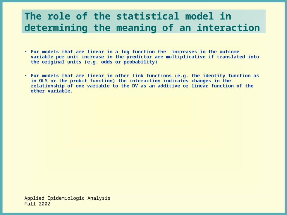
The role of the statistical model in determining the meaning of an interaction

• For models that are linear in a log function the increases in the outcome variable per unit increase in the predictor are multiplicative if translated into the original units (e.g. odds or probability)

• For models that are linear in other link functions (e.g. the identity function as in OLS or the probit function) the interaction indicates changes in the relationship of one variable to the DV as an additive or linear function of the other variable.


Statisticians differ from researchers

Statistician– Uses mathematical probability models to determine what

kind of mathematical treatment of data will produce proper standard errors

– Whether the model estimates reflect how “nature” works is not her problem.

Researcher– Goal is understanding the phenomena being studied. – Check the data for conformity to the assumptions – Should be cautious in changing data to fit the statistical

requirements. – Also needs caution in the interpretations whenever the

assumptions of the model may not fit the substantive problem.


Epidemiological practices that can help identify the model that best represents the data

• Examination of changes in relationships across strata

If your sample is large enough, can get OR or other measures of effect by strata.

Often examine trends in OR across ordinal strata by age.Such an examination would also reveal the shape of a

conditional effect: Does it change as a multiplicative function of the other variable?

• Alternative categorizations of some variables in order to see conditionality.


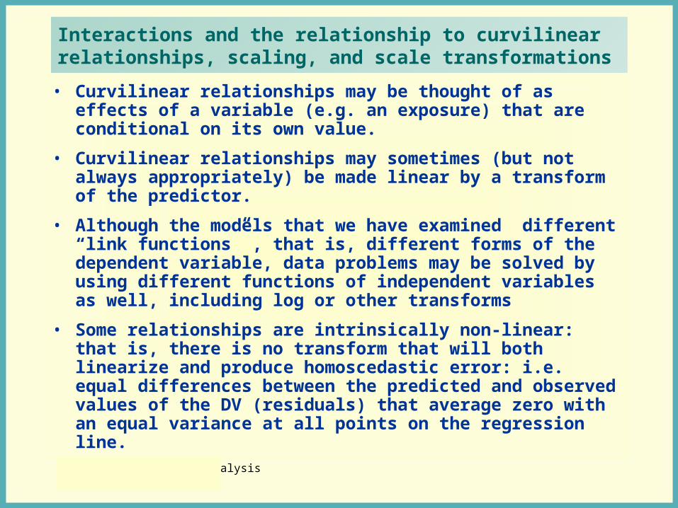
Interactions and the relationship to curvilinear relationships, scaling, and scale transformations

• Curvilinear relationships may be thought of as effects of a variable (e.g. an exposure) that are conditional on its own value.

• Curvilinear relationships may sometimes (but not always appropriately) be made linear by a transform of the predictor.

• Although the models that we have examined different “link functions” , that is, different forms of the dependent variable, data problems may be solved by using different functions of independent variables as well, including log or other transforms

• Some relationships are intrinsically non-linear: that is, there is no transform that will both linearize and produce homoscedastic error: i.e. equal differences between the predicted and observed values of the DV (residuals) that average zero with an equal variance at all points on the regression line.


Interaction effects in OLS

Interactions among categorical variables (e.g. strata)• What you are examining depends on how you coded the

categories.• Most epidemiological studies code strata with dummy variable

coding but that is not always optimal.

• Other methods of coding categorical variables may be more appropriate to one’s hypotheses, and more statistically powerful.


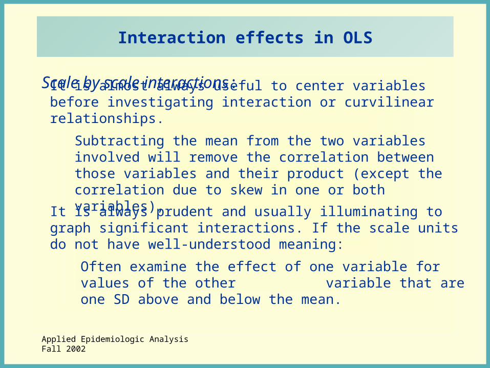
Interaction effects in OLS

Scale by scale interactions:

It is almost always useful to center variables before investigating interaction or curvilinear relationships.

Subtracting the mean from the two variables involved will remove the correlation between those variables and their product (except the correlation due to skew in one or both variables),

It is always prudent and usually illuminating to graph significant interactions. If the scale units do not have well-understood meaning:

Often examine the effect of one variable for values of the other variable that are one SD above and below the mean.


Suppose we had the following analytic findings in an OLS analysis

Y Mean = 5 , Range - 6.5 to 20

E1 Mean = 3 SD = 1.5

E2 Mean = 7 SD = 3

Regression equationY = 1.778 + .290 (E1) + .336 (E2) R2 = .198

Adding the interaction of E1 and E2Y = 8.538 -1.938 (E1) -.663 (E2) + .327 (E1E2)R2 = .546


Graphing this relationship

Y = 8.538 -1.938 (E1) -.663 (E2) + .327 (E1xE2)

We are going to plot two lines. One will represent those cases with an E1 one SD below the mean. The other will be one SD above the mean.

For each line, we choose two arbitrary points for E2 (because 2 calculated points will define a straight line).


Graphing Y = 8.538 -1.938 (E1) -.663 (E2) + .327 (E1E2)

First, for E1 when it is one standard deviation below the mean:

E1 mean = 3 SD = 1.5Low E1 = 3 – 1.5 = 1.5Arbitrary values for E2 6, 8

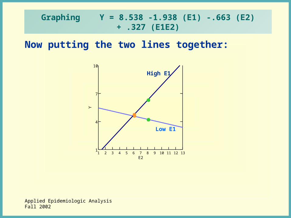
Point 2 Y = 8.538 -1.938 (1.5) -.663 (8) + .327 (1.5 * 8 ) = 4.251

Point 1 Y = 8.538 -1.938 (1.5) -.663 (6) + .327 (1.5 * 6 ) = 4.596

1 2 3 4 5 6 7 8 9 10 11 12 13E2

1

4

7

10

Y


Graphing Y = 8.538 -1.938 (E1) -.663 (E2) + .327 (E1E2)

Now, for E1 when it is one standard deviation above the mean:

HighE1 = 3 + 1.5 = 4.5 E2 arbitrary points 6, 8

Point 2 Y = 8.538 -1.938 (4.5) -.663 (8) + .327 (4.5 * 8) = 6.285

1 2 3 4 5 6 7 8 9 10 11 12 13E2

1

4

7

10

Y

Point 1 Y = 8.538 -1.938 (4.5) -.663 (6) + .327 (4.5 * 6) = 4.668


Now putting the two lines together:

Graphing Y = 8.538 -1.938 (E1) -.663 (E2) + .327 (E1E2)

1 2 3 4 5 6 7 8 9 10 11 12 13E2

1

4

7

10

Y

Low E1

High E1


Centering the variables

Suppose we center the E1 and E2 variables by subtracting the mean from each value.

– We then also use the product of these centered variables to represent the interaction.

– Doing so has absolutely no effect on the relationship of these variables to Y.

– However, it will make the interaction term (almost) uncorrelated with the ‘main effects,’ that is, the centered E1 and E2.

Equation for these centered variables is:

Y = 4.948 + .351 * E1c + .318 * E2c + .327 * E1c E2c

Note that the value for the interaction term remains the same: this will always be the case for the highest order interaction term in the model.


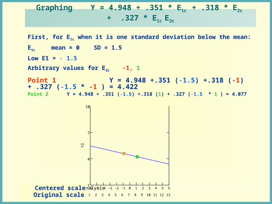
Graphing Y = 4.948 + .351 * E1c + .318 * E2c + .327 * E1c E2c

First, for E1c when it is one standard deviation below the mean:

E1c mean = 0 SD = 1.5

Low E1 = - 1.5

Arbitrary values for E2c -1, 1

Point 2 Y = 4.948 + .351 (-1.5) +.318 (1) + .327 (-1.5 * 1 ) = 4.077

Point 1 Y = 4.948 +.351 (-1.5) +.318 (-1) + .327 (-1.5 * -1 ) = 4.422

1 2 3 4 5 6 7 8 9 10 11 12 13

Centered scaleOriginal scale

-6 -5 -4 -3 -2 -1 0 1 2 3 4 5 61

4

7

10

Y2


Graphing Y = 4.948 + .351 * E1c + .318 * E2c + .327 * E1c E2c

Now, for E1c when it is one standard deviation above the mean:

E1c mean = 0 SD = 1.5

High E1 = 1.5

Arbitrary values for E2c -1, 1

Point 2 Y = 4.948 + .351 (-1.5) +.318 (1) + .327 (1.5 * 1 ) = 6.283

Point 1 Y = 4.948 +.351 (1.5) +.318 (-1) + .327 (1.5 * -1 ) = 4.666

1 2 3 4 5 6 7 8 9 10 11 12 13

Centered scaleOriginal scale

-6 -5 -4 -3 -2 -1 0 1 2 3 4 5 61

4

7

10

Y

Low E1

High E1


Centered

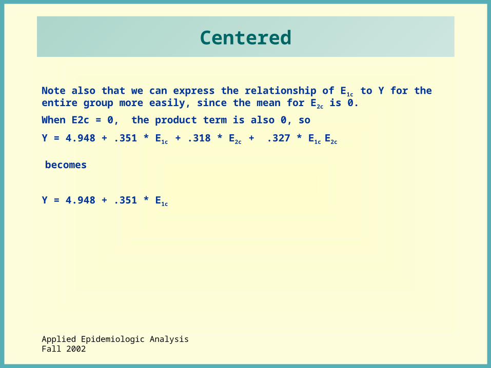
Note also that we can express the relationship of E1c to Y for the entire group more easily, since the mean for E2c is 0.

When E2c = 0, the product term is also 0, so

Y = 4.948 + .351 * E1c + .318 * E2c + .327 * E1c E2c

becomes

Y = 4.948 + .351 * E1c


Alternative means of coding categorical variables to examine and test interactions

• One of the problems when we have a serious interest in conditional relationships is the relatively low statistical power such analyses often have.

• This means we need to do everything possible to increase our statistical power to find such a relationship.

• One methodological way to increase statistical power is to represent categorical data in the analyses in the form most likely to represent these changes in relationship.


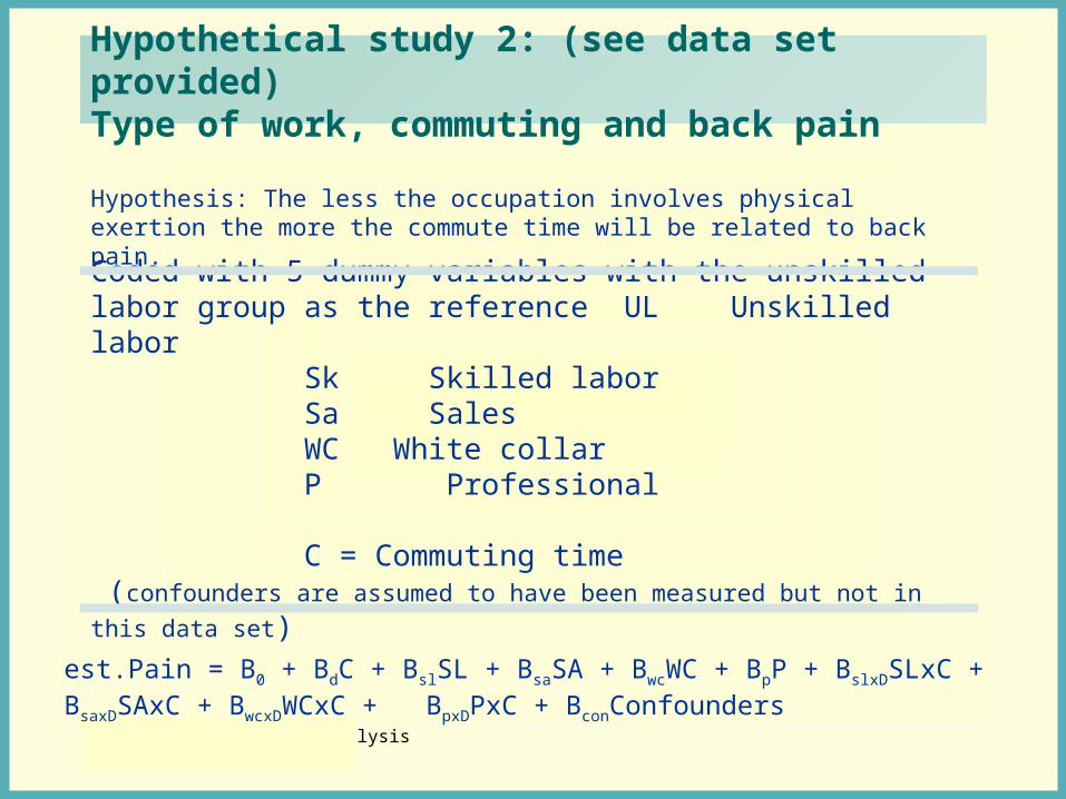
Hypothetical study 2: (see data set provided)Type of work, commuting and back pain

Hypothesis: The less the occupation involves physical exertion the more the commute time will be related to back pain.

Coded with 5 dummy variables with the unskilled labor group as the reference UL Unskilled labor

Sk Skilled laborSa SalesWC White collarP Professional

C = Commuting time (confounders are assumed to have been measured but not in this data set)

est.Pain = B0 + BdC + BslSL + BsaSA + BwcWC + BpP + BslxDSLxC + BsaxDSAxC + BwcxDWCxC + BpxDPxC + BconConfounders


Suppose that we have coded the occupational categories as dummy variables with unskilled labor as the reference

• OD1 = Unskilled labor = 1, otherwise = 0• OD2 = Skilled labor = 1, otherwise = 0• OD3 = Sales = 1, otherwise = 0• OD4 = White collar = 1, otherwise = 0• OD5 = Professional = 1, otherwise = 0

• Remember that we always need one fewer variables than there are groups to represent all the categories (there are g – 1 df)

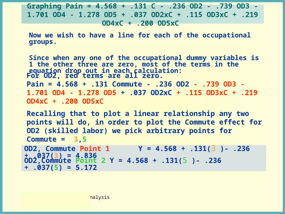
• estPain = 4.568 + .131 Commute - .236 OD2 - .739 OD3 - 1.701 OD4 -• 1.278 OD5 + .037 OD2xC + .115 OD3xC + .219 OD4xC + .200 OD5xC

• R2 = .128


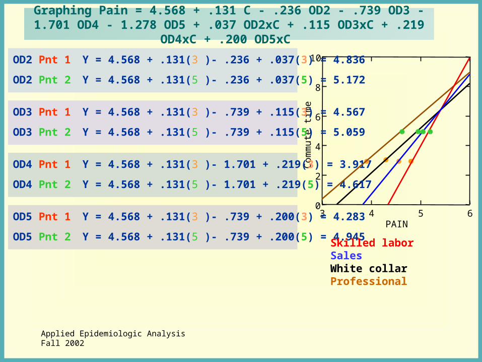
Graphing Pain = 4.568 + .131 C - .236 OD2 - .739 OD3 - 1.701 OD4 - 1.278 OD5 + .037 OD2xC + .115 OD3xC + .219 OD4xC + .200 OD5xC

Now we wish to have a line for each of the occupational groups.

Since when any one of the occupational dummy variables is 1 the other three are zero, most of the terms in the equation drop out in each calculation:

OD2, Commute Point 1 Y = 4.568 + .131(3 )- .236 + .037(3) = 4.836

For OD2, red terms are all zero. Pain = 4.568 + .131 Commute - .236 OD2 - .739 OD3 - 1.701 OD4 - 1.278 OD5 + .037 OD2xC + .115 OD3xC + .219 OD4xC + .200 OD5xC

Recalling that to plot a linear relationship any two points will do, in order to plot the Commute effect for OD2 (skilled labor) we pick arbitrary points for Commute = 3,5

OD2,Commute Point 2 Y = 4.568 + .131(5 )- .236 + .037(5) = 5.172


3 4 5 6PAIN

0

2

4

6

8

10

Com

mut

e tim

e

OD4 Pnt 1 Y = 4.568 + .131(3 )- 1.701 + .219(3) = 3.917

OD4 Pnt 2 Y = 4.568 + .131(5 )- 1.701 + .219(5) = 4.617

OD5 Pnt 1 Y = 4.568 + .131(3 )- .739 + .200(3) = 4.283

OD5 Pnt 2 Y = 4.568 + .131(5 )- .739 + .200(5) = 4.945

Graphing Pain = 4.568 + .131 C - .236 OD2 - .739 OD3 - 1.701 OD4 - 1.278 OD5 + .037 OD2xC + .115 OD3xC + .219 OD4xC + .200 OD5xC

OD2 Pnt 1 Y = 4.568 + .131(3 )- .236 + .037(3) = 4.836

OD2 Pnt 2 Y = 4.568 + .131(5 )- .236 + .037(5) = 5.172

OD3 Pnt 1 Y = 4.568 + .131(3 )- .739 + .115(3) = 4.567

OD3 Pnt 2 Y = 4.568 + .131(5 )- .739 + .115(5) = 5.059

Skilled laborSalesWhite collarProfessional


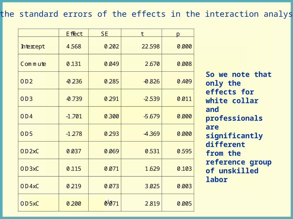
Effect SE t p

Intercept 4.568 0.202 22.598 0.000

Commute 0.131 0.049 2.670 0.008

OD2 -0.236 0.285 -0.826 0.409

OD3 -0.739 0.291 -2.539 0.011

OD4 -1.701 0.300 -5.679 0.000

OD5 -1.278 0.293 -4.369 0.000

OD2xC 0.037 0.069 0.531 0.595

OD3xC 0.115 0.071 1.629 0.103

OD4xC 0.219 0.073 3.025 0.003

OD5xC 0.200 0.071 2.819 0.005

So we note that only the effects for white collar and professionals are significantly different from the reference group of unskilled labor

And the standard errors of the effects in the interaction analyses:


An alternative way of getting these graphs which is easier, and whichprovides a standard error for the slope of each group is accomplishedby the following method of coding for the simple slopes

Omit the main effect for the scaled variable and include all gInteractions between the scaled variable and the dummy variables.

For our illustration this results in the following equation:

Using simple slopes

Here we can determine readily which slopes are significantly greater than zero.

Pain = 5.091 - .089 OD2 - .279 OD3 - .824 OD4 - .477OD5 + .131 OD1xC + .168 OD2xC + .246 OD3xC + .350 OD4xC + .331 OD5C


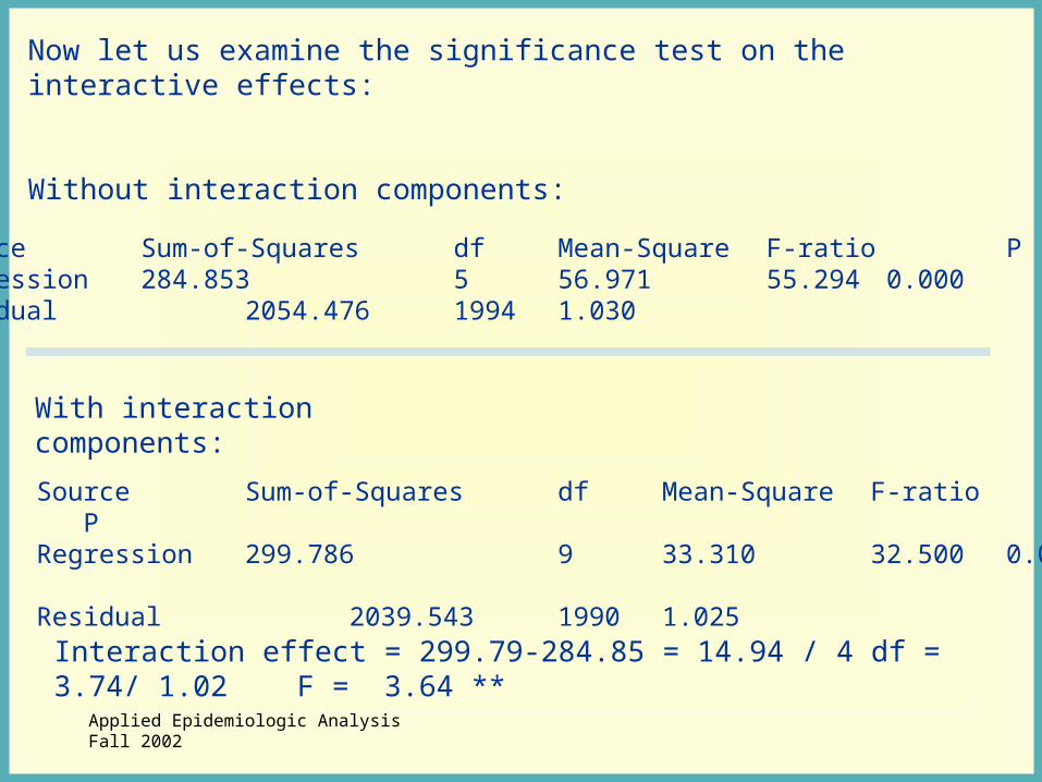
Now let us examine the significance test on the interactive effects:

Without interaction components:

Source Sum-of-Squares df Mean-Square F-ratio PRegression 299.786 9 33.310 32.500 0.000Residual 2039.543 1990 1.025

Source Sum-of-Squares df Mean-Square F-ratio PRegression 284.853 5 56.971 55.294 0.000Residual 2054.476 1994 1.030

With interaction components:

Interaction effect = 299.79-284.85 = 14.94 / 4 df = 3.74/ 1.02 F = 3.64 **


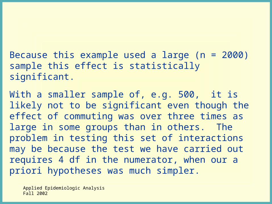
Because this example used a large (n = 2000) sample this effect is statistically significant.

With a smaller sample of, e.g. 500, it is likely not to be significant even though the effect of commuting was over three times as large in some groups than in others. The problem in testing this set of interactions may be because the test we have carried out requires 4 df in the numerator, when our a priori hypotheses was much simpler.


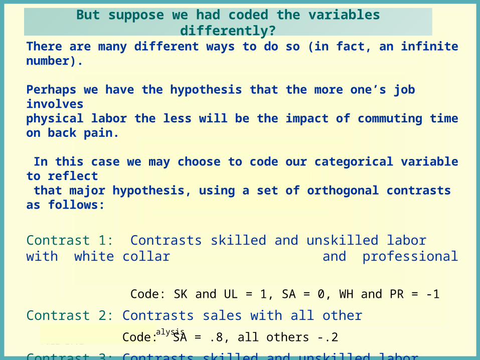
There are many different ways to do so (in fact, an infinite number).

Perhaps we have the hypothesis that the more one’s job involvesphysical labor the less will be the impact of commuting time on back pain.

In this case we may choose to code our categorical variable to reflect that major hypothesis, using a set of orthogonal contrasts as follows:

Contrast 1: Contrasts skilled and unskilled labor with white collar and professional

Code: SK and UL = 1, SA = 0, WH and PR = -1

Contrast 2: Contrasts sales with all other

Code: SA = .8, all others -.2

Contrast 3: Contrasts skilled and unskilled labor

Code: UL = -.5, SK=.5, all others =0

Contrast 4: Contrasts while collar and professional

Code: WH = -.5, PR=.5, all others = 0

But suppose we had coded the variables differently?


Effects and their standard errors for the new codes

Effect Coefficient Std Error

CONSTANT 4.758 0.023

COMMUTEC 0.245 0.023

OCONT1 -0.303 0.025

OCONT2 0.069 0.057

OCONT3 -0.089 0.072

OCONT4 0.347 0.072

OCCOM1 0.096 0.025

OCCOM2 0.001 0.057

OCCOM3 0.037 0.069

OCCOM4 -0.019 0.074

Note that only the first contrast reflects our a priori hypothesis.

In subsequent analyses we may reasonably remove the last threecontrasts from consideration, their presence being only a check on thelimits of our hypothesis.


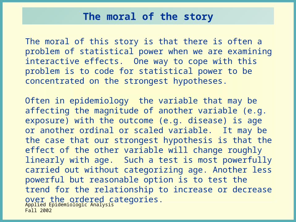
The moral of this story is that there is often a problem of statistical power when we are examining interactive effects. One way to cope with this problem is to code for statistical power to be concentrated on the strongest hypotheses.

Often in epidemiology the variable that may be affecting the magnitude of another variable (e.g. exposure) with the outcome (e.g. disease) is age or another ordinal or scaled variable. It may be the case that our strongest hypothesis is that the effect of the other variable will change roughly linearly with age. Such a test is most powerfully carried out without categorizing age. Another less powerful but reasonable option is to test the trend for the relationship to increase or decrease over the ordered categories.

The moral of the story


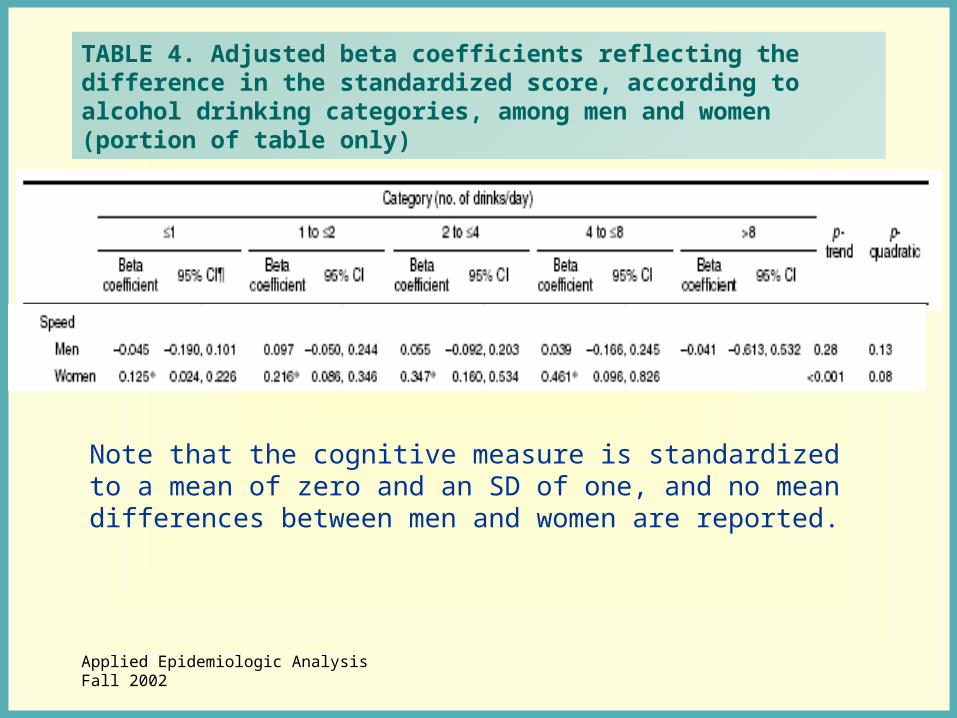
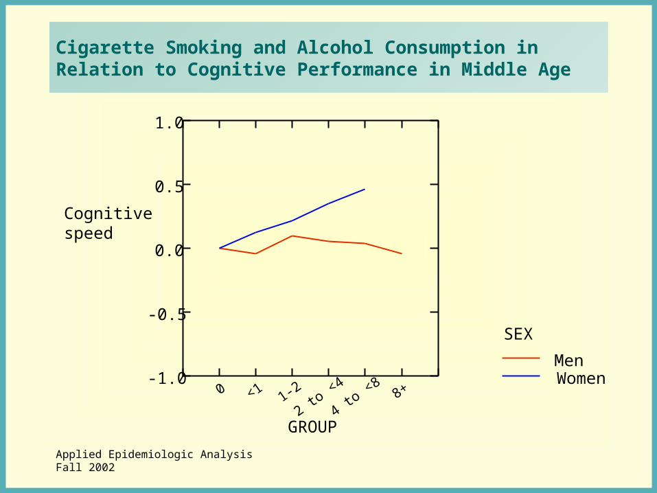
Cigarette Smoking and Alcohol Consumption in Relation to Cognitive Performance in Middle Age

Sandra Kalmijn, Martin P. J. van Boxtel, Monique W. M. Verschuren, Jelle Jolles, and Lenore J. Launer, American Journal of Epidemiology, 156, 936-944.

Goals of the study: to determine the relationship between smoking history (pack years), alcohol consumption, and cognitive function in men and women at an average age of 56. N = 1,947 participants from the Netherlands.

Findings: Primary differences were in speeded tests, for which negative effects were found for current smoking, and an interaction between sex and alcohol consumption.


TABLE 4. Adjusted beta coefficients reflecting the difference in the standardized score, according to alcohol drinking categories, among men and women (portion of table only)

Note that the cognitive measure is standardized to a mean of zero and an SD of one, and no mean differences between men and women are reported.


0 <1 1-22 to

<4

4 to <8 8+

GROUP

-1.0

-0.5

0.0

0.5

1.0

Cognitive speed

WomenMen

SEX

Cigarette Smoking and Alcohol Consumption in Relation to Cognitive Performance in Middle Age


Interactions involving 3 or more predictors

• Even if you have a number of predictors, an important interaction should be at least faintly visible at some categorical level involving the IVs and the DV (if the DV is a scale, use mean scores).

• If a study is really intended to find an hypothesized triple interaction, statistical power problems should be taken very seriously in both the study design and in the analysis.


Interaction effects in logistic regression

• The link function connecting the dependent variable and the sum of weighted independent variables is the logit or log odds of outcome.

• In order to translate back into the original units of the DV, we exponentiate both sides of the equation.

• The predicted odds of the DV (e.g. disease) = sum of the products of the exponentiated weighted risks.

• When interactions involve different effects in different populations (e.g., sex or age groups), interactions are generally examined by displaying effects such as the OR for the exposure in each stratum.


Low-Dose Exposure to Asbestos and Lung Cancer: Dose-Response Relations and Interaction with Smoking in a Population-based Case-Referent Study in Stockholm, Sweden

Per Gustavsson, Fredrik Nyberg, Göran Pershagen, Patrik Schéele, Robert Jakobsson, and Nils Plato, American Journal of Epidemiology, 155, 1016-1022.

Study goals: Determination of whether there was a synergistic effect of asbestos and smoking on the risk of lung cancer.

Study sample: 1038 incident male lung cancer cases in Sweden and 2359 referents matched on age and inclusion year for whom occupational exposures were determined.

Findings: Lung cancer risk increased almost linearly with cumulative dose of asbestos rather than exponentially as predicted by the logistic model. To remedy this the asbestos doses were transformed logarithmically (dose = ln(fiber-years +1). For smoking the dose response was between linearity and exponentiality and the smoking measure was transformed to the square root of grams/day, which fit much better.


Low-Dose Exposure to Asbestos and Lung Cancer


Low-Dose Exposure to Asbestos and Lung Cancer

• Subsequent analyses using various functions of the two exposure variables all showed that the effect of the interaction (product) was less than one (e.g. OR = .85 with confidence limits not including 1.0), indicating that the combination of the two risks did not have the multiplicative effect assumed by the logistic model, although it was more than additive.

(Note: they did not show this graphically)


Interaction effects in multilevel logistic regression

For longitudinal data the clusters represent the multiple assessments of individual respondents. The interactional questions that may be asked of these data include the following:

To what extent are the changes over time conditional on some stable characteristic of the respondents?

Does the relationship between the (changing) outcome variable and some (changing) predictor vary as a function of some characteristic of the respondents?

In each of these analyses the principles of centering and graphing continue to be critical to understanding the findings.