applications of nonlinear models in contribution margin

Journal of Business Cases and Applications Volume 16

Applications of Nonlinear Models in Contribution Margin and

Profit Analysis

Di Wu California State University-Bakersfield

Ji Li

California State University-Bakersfield

ABSTRACT

Management of a company often needs to make business decisions such as make-or-buy, sell-or-process- further and maximization of contribution margins based on available accounting information of revenues, costs and resource constraints. To find optimal solutions, mathematical models, such as linear and non-linear models, can be applied. Linear models are particularly of interest due to their simplicity and convenience. However, in practice with complex product designs and complicated business operations, some linear models do not do a thorough job of analyzing the relationships between the objectives and independent variables; they may also provide false results. Therefore, nonlinear models are sometimes believed to simulate business operations better in practice, enabling business professionals to make more accurate decisions. Given the complex nature of nonlinear models, accountants who favor simplicity are hence reluctant to apply them. The objective of this paper is to introduce several theories and methods of nonlinear models that can be directly applied to study complex cost and managerial accounting issues, such as maximizing contribution margins and profits. Furthermore, this paper elaborates on how to use Excel toolboxes to solve applied nonlinear models. By using these Excel toolboxes, accountants can simplify quantitative modeling in cost and managerial accounting issues and avoid complicated computational steps.

Keywords: Accounting Education, Contribution Margin, Nonlinear Models, Regression, Optimization, Excel Toolboxes.

Copyright statement: Authors retain the copyright to the manuscripts published in AABRI journals. Please see the AABRI Copyright Policy at http://www.aabri.com/copyright.html


Introduction

Cost and managerial accounting deals with accounting information obtained from either historical records or predictions so that management can make decisions on the budgeting and allocation of resources with purposes of minimizing operating expenses, maximizing profits or contribution margins, and minimizing costs of financing (Horngren 2015). Many applied models focus on linear models with or without linear constraints, which simplifies calculations and allows users to easily implement these models in their applications (Togo, 2008). Linear programming methods (e.g., simplex method, integer programming, quadratic programming and binary programming) can be used to solve these models (Chvatal, 1983).

From optimization and practical perspectives, it can be seen that the applications of mathematical models in cost and managerial accounting have wide and important impacts on the understanding of business operations. Given complex product designs, manufacturing processes and operations, linear models may not always be able to provide an accurate analysis. Managers who are limited to using linear models may not gain the insights of business operations accurately. Therefore, accountants may often need to consider nonlinear models even with nonlinear constraints.

Marketing researchers often observe that the selling price has an effect on the number of products sold. As such, it can be said that customers can be very price sensitive to certain products and that there might be a nonlinear correlation between the selling price and the sales in units (Landsburg, 2013). Production managers know that learning curves may need to be considered in the productivity analysis and director labor costs. Therefore, direct labor costs per unit, which is a variable cost per unit, may decrease as more products are manufactured and sold (Horngren 2015). In many of these fields, nonlinear models might be better used than linear models.

Many accounting education curriculums or textbooks, including those at the undergraduate and graduate MBA levels, seem to focus more on linear models; little introduction is given to nonlinear models. Consequently, this paper will provide a general overview of some nonlinear models with their applications in cost and managerial accounting to help managers determine the optimal value of business operations (e.g., contribution margins and profits). This overview is not limited to pricing, the allocation of resources for product-mixes, the cost of financing and managing inventory level, and the optimization of the return on investment. This is because, in addition to optimizing business objectives, business professionals are also interested in understanding the characteristics of modeled business operations and predicting future outcomes using mathematical models.

In general, due to the complexity of business operations, some mathematical models may not have optimal solutions or may have more than one optimal solutions in terms of business objectives. Therefore, pretests or previews of applied quantitative models become very important to avoid any misunderstanding or false information. Sensitivity analysis is a very useful tool which fixes most variables, but relaxes a few, so that managers or accountants can experiment with different conditions that yield different outcomes. However, sensitivity analysis is more like a trial-or-error method and less effective when the operations are complex and contain many variables (Drury, 2007).

With advancements in computer technology and accounting software packages, accountants have greater opportunities now than ever to study more sophisticated business operations and use computer technology to apply complicated nonlinear models in the analysis


of accounting information. Even without advanced knowledge in multivariate calculus, linear programming and numerical optimization methods, accountants are able to find optimal solutions easily through computer software packages, including Excel toolboxes, SPSS and SAS. Big data and information technology have made revolutionary changes in some accounting subjects and will continue to assist business professionals in making business decisions and using business resources more effectively and efficiently (Warren, 2015).

Mathematical models and optimization methods

Modeling cost and managerial accounting questions can be classified into two categories: linear and nonlinear models. With linear models, most variables are expressed up to the first degree and can easily find optimal solutions for defined objective functions. Nonlinear models are more difficult to apply. As such, this paper focuses on the application of nonlinear models in contribution margin and profit analysis. Management accounting defines variable costs to be ones that change in total in proportion to change in the volume (Horngren, 2015). This paper focuses more on nonlinear variable costs whose changes are not directly proportional to changes in volume. So variable costs in the rest of paper really mean nonlinear variable costs. Definitions

Linear Model - A linear model is a function that can be expressed in the following form:

n

nnn RDxxxxxcxcxcxf ⊆∈=+++= D,x ),,...,,( where,...)( 212211 (1)

Any function that cannot be expressed in the form of Equation (1) is a nonlinear model. Objective Function - An objective function is a linear or nonlinear function that needs to be maximized or minimized on its domain, such that:

n

nDx

RDxxxxxf ⊆=∈

),,...,,( where,)(min/max 21 (2)

Relevant Range - Relevant range is a specific operation or activity level which is bounded between a maximum or minimum value given the resource constraints.

*x - *x is said to be an absolute maximizer (minimizer) to a function )(xf if )(*)( xfxf ≥

( )(*)( xfxf ≤ ) for any Dx ∈ , n

n RDxxxx ⊆= ),,...,,( where 21 .

Critical Value of Function - A critical value of function )(xf is defined to be a value where the

derivative of )(xf , say )(' xf , equals 0 or does not exist.

Many management decisions intend to maximize contribution margins, profits or returns

on assets/equity/investments. Typically, cost or managerial accountants can model objective functions in business operations, say, by defining profit functions by using a revenue function subtracted by a cost function. Optimization methods can then be applied to find the maximum profit value and its optimizer.

It is interesting to see that many studies show that the selling price per unit and sales in units are highly related (Landsburg, 2013). Generally, when the selling price drops, more products will be sold; however, when the unit price rises, fewer products will be sold. Depending


on the elasticity, the price effects can range from little to substantial. In the meanwhile, the sales in units will consequently affect the total inventorial costs and costs of goods sold.

Assume that a company sells n products and each product has a relationship between the selling price and sales in units. The number of units normally depends on the product selling price. However, for a convenient application, in this paper, the product selling price will be

expressed in terms of the number of units sold. For instance, let: nxxx ,...,, 21 be the number of

units sold for each of the n products, )(),...,(),( 2211 nm xpxpxp be the corresponding price,

nDDD ,...,, 21 be the relevant range for each product manufactured, )(),...,(),( 2211 nn xvcxvcxvc be

the unit variable cost function for each unit product manufactured, and finally, fc be the total

fixed cost function, which is constant within the relevant range. Considering these definitions, the profit function can be modeled as:

[ ]∑ −−=i

iiiii fcxvcxpxxf )))()((()( , where n

nn RDDDDDxxxx ⊂=∈= ,),...,,(),...,,( 2121

(3)

Note that )()( iiii xvcxp − is also called the contribution margin per unit.

Theorem 1. A company has modeled its profit function, as illustrated in (3). If D is closed and

)(xf is a continuous function, then )(xf has an absolute maximum value at *xx = such that

)(*)( xfxf ≥ for all Dx ∈ .

Proof. The proof is beyond the scope of cost and managerial accounting subject, but it is illustrated in Wade (2010). Furthermore, a cost function can be divided into a variable cost component and a fixed cost component. Within the relevant range, the fixed cost component is normally constant. From optimization perspectives, an optimal solution to a derived profit function in cost and managerial accounting is also an optimal solution to its derived contribution margin function. For instance, as the above example shows, the contribution margin is expressed as Equation (4) and (5):

[ ] fcxvcxpxfcxCMxfi

iiiii −−=−= ∑ )))()((()()( (4)

[ ] fcxfxvcxpxxCMi

iiiii +=−= ∑ )()))()((()( (5)

Theorem2. A company has modeled its profit function and contribution margin function as illustrated in (4) and (5). If the profit function )(xf has an absolute maximum value at *xx = , D

is closed and )(xf is a continuous function, then

[ ]∑ −==+i

iiiii xvcxpxxCMfcxf ))()(()()( has an absolute maximum value at *xx = or, in

other words, the contribution margin function has an absolute maximum value at *xx = .

Proof: If the profit function )(xf has an absolute maximum value at *xx = , it is obvious that

)(*)( xfxf ≥ for all Dx ∈ . Therefore, given a constant fc , the following inequality holds as

well, fcxffcxf +≥+ )(*)( for all Dx ∈ , which is equivalent to saying, )(*)( xCMxCM ≥ for all

Dx ∈ . Hence, it has been proven that )(xCM has an absolute maximum value at *xx = , as

defined.


Mathematically, an optimal solution to a profit function (4) or contribution margin function (5) may not be an integer. However, in the models, these variables represent the numbers of units sold for multiple products, and hence, need to be integers. One way to handle this is to simply round the decimal solutions to obtain integer solutions. These integer values can then be used to estimate the maximum profit or contribution margin. However, this method may not guarantee an absolute maximum value after the using rounded integers. Another way to find integer solutions is more rigorous. It involves using calculus concepts to find the critical values of the profit or contribution margin function. Given that D is closed and

)(xf is a continuously polynomial function, there exists a finite number of critical values of

)(xf . For every noninteger critical value, round it down and up to obtain two integers; this is

called its floor and ceiling. With a finite set of found integers, compare the )(xf values at these

integers to find the maximum value (Stewart, 2013). Numerical optimization methods in cost and managerial accounting

Depending on what models are used in cost and managerial accounting problems, several

techniques can be applied, including linear, integer, binary and mixed-integer programming, quadratic programming, steepest descent, Newton’s method for continuous nonlinear models, and combinatorial optimization methods. This paper focuses on nonlinear models with an application in one product cost accounting problem. A calculus based approach can be applied to find the optimal solution, which is guaranteed and illustrated in the previous theorems. The method used in the study including the following mathematical steps (Stewart, 2013):

1) Define the cost object, such as the product, activity, project and the relevant range

bna ≤≤ .

2) Find the selling price per unit and variable cost per unit to derive the contribution margin per unit.

3) Set up the total contribution margin function )(nf = (selling price per unit – variable

cost per unit) * number of units sold. 4) Differentiate )(nf and then solve bna whereexist,not does or 0)(' ≤≤= f'(n)nf .

Assume that there are m solutions, neither a nor b, to bna where0,)(' ≤≤=nf . There

are then a total of m+2 critical values, including bccca m and ,,...,,, 21 .

5) Evaluate )(nf at all of the critical values and find the largest value of )(nf . The

maximum contribution margin is then determined at the critical value, where )(nf is

largest. Theorems 1 and 2 show that this method and its conditions (i.e., that )(nf is continuous and

bna ≤≤ ) guarantee that )(nf has an absolute maximum value over bna ≤≤ .

Regression analysis in pricing analysis and cost analysis

In order to study the pricing model, which explains the relationship between the unit price and the number of products sold, accountants and market researchers often use a regression analysis (Draper, 1998). If available, accountants start with the unit price and market response to that price, which is reflected in the number of products sold. Accountants can then either obtain data from a marketing analysis or the historical accounting records.


Accountants can apply a regression analysis to fit a model (e.g., linear, exponential, polynomial and logarithmic function) to the collected sales data. To do this, they should select the model with the largest R squared value. Similarly, if the variable cost per unit is not constant, given the purchase discounts offered by suppliers and direct labor costs linked with learning curve models, then a nonlinear model might be applied to study the effects of sales in units on the variable costs per unit. As can be seen, a regression analysis can be applied to model the correlation between the variable cost per unit and the number of products manufactured and sold.

Application of nonlinear models and optimization methods in examples

Electric-Star Company Background

Electric-Star Incorporated is a multinational corporation that manufactures personal

electronics, including portable chargers for smartphones. The company has an annual manufacturing capacity of 1 million portable chargers; within the relevant range, fixed costs remain constant. The marketing department of Electric-Star has conducted research regarding the relationship between the number of units sold and the selling price. As many studies show, customers are very price sensitive to products like portable chargers. When the price is set higher, fewer products will be sold; more products will be sold when the price is set lower. Their marketing department manager John hired a quantitative marketing researcher who applied mathematical models to study their sales in units and the selling price.

Pricing and sales-in-units model

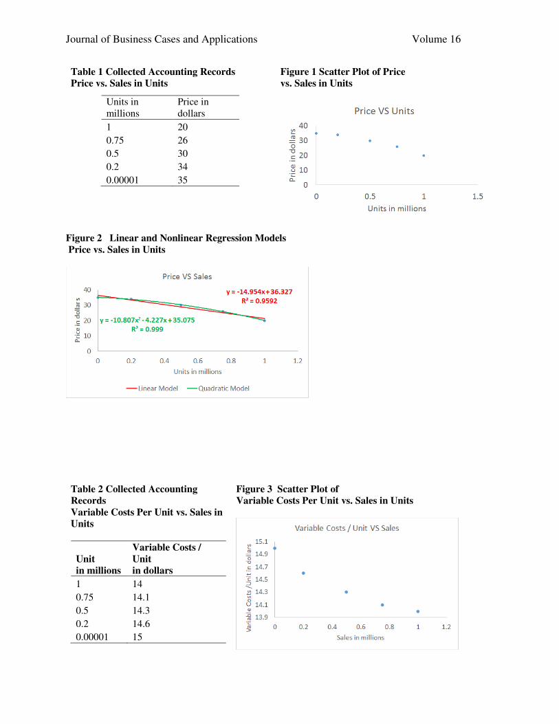
The accountants and sales associates collected historical sales data (Table 1). The data

were collected over several years and present the effects of the sales price on the sales volume (see Table 1 in the appendix); a scatter plot is shown in Figure 1 (appendix).

The accountant is thinking of using a linear regression model to study the price and sales volume function. Based on a further analysis of the marketing data and historical accounting records, John believes a nonlinear model is more appropriate. The accountant and John decide to try both linear and nonlinear models by regression analysis. The results reveal that a nonlinear model has a better fit of the data (see Figure 2 in the appendix).

After a discussion, with the marketing researcher and accountant, John decides to use a nonlinear model for modeling the price and sales volume, since the model has a better fit of the data, as shown in (6), where p is the selling price and n is the number of units sold:

075.35227.4807.10)( 2+−−= nnnp , where n in millions and p in dollars (6)

A newly hired CEO wants to maximum the profit by pricing portable chargers appropriately. John is then asked to obtain the accounting information needed to determine the price which will give the company the highest profit.

Variable cost per unit

The marketing department manager John obtains the price and quantity from the hired

quantitative marketing researcher and accountant. John then asks the production manager and accountant to gather data on the variable cost per unit and the fixed costs. After a detailed analysis, it seems that fixed costs are$3 million and remain constant within the relevant range of


the production of no more than 1 million portable chargers. However, the variable cost per unit is not fixed and depends on the units sold and manufactured. A key point to note is that, in practice, raw material suppliers often offer discounts for large sales, skilled workers pick up learning curves and variable overhead per-unit costs may be reduced when more products are manufactured and sold. The historical data and statistical analysis suggests to John, the production manager and the accountant that the variable cost per unit, including variable manufacturing and variable period costs, is a dependent function of the number of units sold.

The marketing department manager John asks the cost accountant to collect data on the variable costs per unit and sales volume data for further analysis. The data collected are shown in Table 2 (appendix); a scatterplot is shown in Figure 3 (appendix).

John has experience with price and sales volume analysis. He is quite confident that a nonlinear model is better for the study of the relationship between the variable cost per unit and the sales volume data, as shown in Figure 4 (appendix). John still tries both the linear and nonlinear models. The results show that a nonlinear model may be more accurate in modeling the relationship between the variable costs per unit and the sales in units. John decides the nonlinear model is better, as shown in (7), where the variable cost per unit is represented by VC in million dollars and n is the number of units sold in millions:

9768.148268.18593.0)( 2+−= nnnVC , where 1n0 ≤≤ (n in millions), VC in dollars

(7) Contribution Margin

The marketing department manager John first derives and sets up the unit contribution

margin function. The contribution margin per unit equals the selling price per unit minus the variable cost per unit. John then determines that, given the selling price p, the portable charger contribution margin per unit is:

0928.204002.26663.11

)9768.148268.18593.0(075.35227.4807.10)()(2

22

+−−=

+−−+−−=−

nn

nnnnnVCnp (8)

The marketing department manager can then find out the contribution margin in total =

nnn ⋅+−− )0928.204002.26663.11( 2 , where 10 ≤≤ n in millions. John can further determine the

profit, which is the contribution margin, in total, minus the total fixed costs, in millions of dollars:

5)0928.204002.26663.11()( 2−⋅+−−= nnnxg (9)

The marketing department manager can solve an optimization problem of either the contribution margin or the profit function:

1n0 where,)0928.204002.26663.11max( 2≤≤⋅+−− nnn (n in millions)or (10)

1n0 where,5)0928.204002.26663.11max( 2≤≤−⋅+−− nnn (n in millions) (11)

Optimization of the objective function

As Theorems 1 and 2 show, the contribution margin function (10) and profit function

(11) must have an absolute maximum value over its domain 1n0 ≤≤ (n in millions). The advanced calculus based approach steps illustrated previously can be followed to find the


optimal solution for(10) or (11). Note that the optimal solution to (10) is also an optimal solution to (11), and vice versa. Therefore, John can solve either (10) or (11).

John decides to find the maximum value of the contribution margin function:

1n0 where,)0928.204002.26663.11max( 2≤≤⋅+−− nnn (n in millions) (10)

To accomplish this, John can simplify the contribution margin function:

nnn

nnnnf

0928.204002.26663.11

)0928.204002.26663.11()(23

2

+−−=

⋅+−−=(12)

Critical Values

To find the critical values of f(n), one needs to determine the first order derivative of the

contribution margin function,

1n0 where,0928.208004.49989.34)(' 2≤≤+−−= nnnf in millions. The critical

values include solutions to the equation below, in addition to the ending points 0 and 1:

1n0 where0,

0928.208004.49989.34)(')(' 2

≤≤=

+−−== nnnfnf (13)

The solution to 1n0 where0,)(' ≤≤=nf , can be easily determined by solving a

quadratic equation for n, where 1n0 where,69221.0 ≤≤=n . The critical values are 0, 0.69221

and 1.

Optimal solution

The contribution margin can be evaluated at each critical value. The selling price can be

determined using the formula (6). The critical value at which the function value is maximized is the optimal solution. Table 3 (appendix) shows the analysis of these critical values. The marketing department manager John plugs in each critical value into the variable cost function, selling price function, contribution margin function and profit function as shown above.

The analysis shows that the Electric-Star Company will obtain a maximum profit of U.S. $5.89 million when the portable charger selling price per unit is $26.97. John also shows the graph of the contribution margin function in Figure 5 (appendix), which demonstrates that the optimizer is between 0.60 and 0.75units in millions and that the result is consistent with the numerical solution. Excel Toolboxes

The regression analysis and determination of the optimal solution of a continuous function over a closed interval can be conducted by using Excel toolboxes. These Excel toolboxes, or add-on functions, can greatly help accountants to conduct an analysis of complex business operations and make business decisions without going into the many details of advanced calculus, numerical optimization and quantitative modeling. Therefore, accountants may not need to know very much about advanced calculus, numerical computing or data mining and still be able to use sophisticated models to find optimal solutions. The steps to model business operations and find optimal solutions includes defining cost objects, collecting the required accounting data, completing a linear or nonlinear model by regression analysis, setting


up linear or nonlinear objective functions regarding contribution margins, profits and the cost of financing and determining optimal solutions to the objective functions. With the employment of computer technology, these steps can be greatly simplified. Therefore, accountants will then be able to extract accurate and useful information from the analysis of business operations and make wise business decisions. Below, the Excel toolboxes for a regression analysis and optimization problems are illustrated.

Regression analysis

Accountants can start with the collection of data of independent and dependent variables,

input the data into an Excel file with the selected data for a regression analysis, and then, on the top menu, click INSERT ->Scatter -> Scatter, as shown in Figure 6 (appendix). The set of collected data is plotted as a scatter plot in Excel. Users can click on the “+” to pull out “CHART ELEMENTS” and click on “TRENDLINE”, which has many regression options. Click “MORE OPTIONS” to explore many selections, including linear, exponential, power and polynomial models, as shown in Figure 7.

After selecting “MORE OPTIONS” and specifying a particular model, users can then check the boxes of “Display Equation on chart” and “Display R-Squared value on chart”. Users can also explore several models in the same figure to compare their fitness and R-squared values to select the best model for the analysis. The excel output will provide the R-squared values and model expressions for further use, as shown in Figure 8 (appendix). In Figure 8, three models are applied: exponential, linear, polynomial models. Among them, the polynomial model has the largest R-squared value, and hence, should be selected for further analysis.

Excel Optimization Solver

Accountants sometimes need to find the maximum contribution margin or profit to plan business operations, which often requires solving optimization problems. However, for nonlinear models, it can be very complicated to solve optimization problems in traditional ways. The Excel optimization Solver can help accountants skip complicated steps requiring a background in advanced calculus, linear programming and numerical computing to effectively find optimal solutions to continuous models over a closed interval.

To accomplish this, make sure that the Excel Solver is added. To do this, Click FILE -> OPTIONS -> ADD-INS -> MANAGE -> EXCEL ADD-INS -> GO. A pop-up window shows more options. Then click SOLVER ADD-IN -> OK and the Excel Solver is added. Figure 9 shows the initiation of the Excel Solver.

Users then need to input an objective function to be maximized and relevant ranges of independent variables in the Excel Worksheet. To illustrate this, the contribution function and relevant range defined in the above example is used:

1n0 where,)0928.204002.26663.11max( 2≤≤⋅+−− nnn (n in millions)

Figure 10 (appendix) shows the input of the function and relevant range used in the demonstration. To accomplish this task, input the relevant range 1n0 ≤≤ ,n in millions and

note that the coefficient is 1. The Cell B3 is for the variable input n and Cell E3 is for the upper bound 1 in millions. The Cell G6 is for the function expression in terms of the variable input B3.


The function expression nnnnf 0928.204002.26663.11)( 23+−−= is used as the top row

shows in terms of Cell B3. Follow Figure 11's (appendix) illustration to start the solver to find the optimal solution. To do this, click DATA -> SOLVER to start Excel Solver and then input G6 into the “Set Objective”, B3 into “By Changing Variable Cells” and B3 and E3 into “Subject to the Constraints”. Finally, click “Solve” to find the optimal solution.

As the results show, the contribution margin is maximized at 6922.0=n in millions and the maximum contribution margin is $8.89 million, which are exactly the optimal solution and maximum contribution margin found by the advanced calculus method. Hence, using Excel toolboxes is equivalent to applying an advanced calculus method and numerical computing to find the optimal solution and maximum value of the contribution margin function. Accountants without knowledge of advanced calculus and numerical optimization can enjoy Excel toolboxes to solve optimization problems.

Summary and Conclusions

This paper introduces how to employ nonlinear models in regression analysis to optimize business objectives with available accounting data. It also shows how to use computer technology to facilitate accurate business decision making and manage business operations effectively and efficiently. Using the method introduced in this study, accountants who are lacking in a background in advanced calculus and numerical optimization techniques can rely on computer software to approach sophisticated business operating problems.

A company like Electric-Star can model the selling price, number of units sold and variable cost per unit with nonlinear regression models. In practice, nonlinear models are supplementary or sometimes necessary due to their complex product design, sophisticated manufacturing processes and advanced business operations. An advanced calculus approach and numerical optimization methods have assisted Electric-Star to conduct a more sophisticated pricing regime and cost analysis to generate larger profits. Mathematical theories can guarantee the existence of optimal solutions when certain conditions are satisfied in particular models. Excel Regression and Solver functions can overcome the technical challenges, model business operations and solve optimization problems effectively and efficiently.

Accounting students or professionals can easily apply regression analysis toolboxes in Excel to study accounting information to obtain insights into business operations. In particular, they are able to use Excel toolboxes to model supply, demand, pricing, variable costs, manufacturing activities, and contribution margins with nonlinear models. Given modern complex business operations, many models used to study contribution margins, pricing and costs may not be necessarily as simple as linear functions. Using more accurate and sophisticated nonlinear models, management can better plan business operations and make more accurate business decisions.

In summary, accounting professionals should be prepared to deal with more sophisticated models, including nonlinear models. Understanding and being able to expertly apply computer technology, such as Excel Regression and Solver toolboxes, can greatly improve business profits.


References

Charles Thomas Horngren, George Foster, and Srikant M. Datar, Cost Accounting, 15th Edition, Pearson, 2015

Dennis F. Togo, Amaya Company: Financial Considerations For Product-Mix LP Models, Journal of Business Case Studies Vol 4, No 11 (2008)

Vasek Chvatal, Linear Programing, W H Freeman & Co (Sd), 1983 Steven Landsburg, Price Theory and Applications, South-Western College Pub, 2013 Colin Drury, Management and Cost Accounting, Cengage Learning Business Press, 2007 J. Donald Warren Jr., Kevin C. Moffitt, and Paul Byrnes (2015) How Big Data Will Change

Accounting. Accounting Horizons: June 2015, Vol. 29, No. 2, pp. 397-407. William R. Wade, An Introduction to Analysis, 4th ed., Pearson Prentice Hall, Upper Saddle

River, NJ, 2010 Jorge Nocedal, Stephen Wright, Numerical Optimization, Springer, 2006 James Stewart, Multivariable Calculus, Cengage Learning, 7 edition, 2013 Norman R. Draper, Harry Smith, Applied Regression Analysis, 3rd edition, Wiley, 1998


Table 1 Collected Accounting Records

Price vs. Sales in Units

Units in millions

Price in dollars

1 20

0.75 26

0.5 30

0.2 34

0.00001 35

Figure 1 Scatter Plot of Price

vs. Sales in Units

Figure 2 Linear and Nonlinear Regression Models

Price vs. Sales in Units

Table 2 Collected Accounting

Records

Variable Costs Per Unit vs. Sales in

Units

Unit

in millions

Variable Costs /

Unit

in dollars

1 14

0.75 14.1

0.5 14.3

0.2 14.6

0.00001 15

Figure 3 Scatter Plot of

Variable Costs Per Unit vs. Sales in Units


Figure 4 Linear and Nonlinear Models by Regression

Variable Costs Per Unit vs. Sales in Units

Table 3 Formulas, Critical Values and Contribution Margin

Accounting value Model

Variable cost function 9768.148268.18593.0)( 2+−= nnnVC

Selling price function 075.35227.4807.10)( 2+−−= nnnp

Contribution margin function nnnnf 0928.204002.26663.11)( 23+−−=

Profit function 5)0928.204002.26663.11()( 2−⋅+−−= nnnxg

Critical Value 0 in millions 0.69221 in millions 1 in millions

Variable cost/Unit 14.98 in USD 14.12 in USD 14.01 in USD Selling price/Unit 35.08 in USD 26.97 in USD 20.04 in USD Contribution margin 0 in millions USD 8.89 in millions of USD 6.03 in millions of USD Profit -3 in millions USD 5.89 in millions of USD 3.03 in millions of USD Conclusion Maximum


Figure 5 Graphical Demonstration

Figure 6 Input Collected Data and Scatter Plot

Figure 7 Initiation of Regression Analysis

0

2

4

6

8

10

0 0.2 0.4 0.6 0.8 1 1.2

Co

ntr

ibu

tio

n M

arg

in

Units in millions

Contribution Margin ($ millions)


Figure 8 Regression Analysis with Several Models

Figure 9 Initiation of Excel Solver


Figure 10 Input Function and Relevant Range

Figure 11 Using Solver to Find the Optimal Solution

applications of nonlinear models in contribution margin

Documents