applications of monte carlo methods to statistical...
TRANSCRIPT

Rep. Prog. Phys.60 (1997) 487–559. Printed in the UK PII: S0034-4885(97)55209-2
Applications of Monte Carlo methods to statistical physics
K BinderInstitut fur Physik, Johannes Gutenberg-Universitat Mainz, Staudingerweg 7, D-55099 Mainz, Germany
Received 3 December 1996
Abstract
An introductory review of the Monte Carlo method for the statistical mechanics of condensedmatter systems is given. Basic principles (random number generation, simple samplingversus importance sampling, Markov chains and master equations, etc) are explained andsome classical applications (self-avoiding walks, percolation, the Ising model) are sketched.The finite-size scaling analysis of both second- and first-order phase transitions is describedin detail, and also the study of surface and interfacial phenomena as well as the choiceof appropriate boundary conditions is discussed. Only brief comments are given on topicssuch as applications to dynamic phenomena, quantum problems, and recent algorithmicdevelopments (new sampling schemes based on reweighting techniques, nonlocal updating,parallelization, etc). The techniques described are exemplified with many illustrativeapplications.
0034-4885/97/050487+73$59.50c© 1997 IOP Publishing Ltd 487

488 K Binder
Contents
Page1. Introduction 4892. Random number generation and simple sampling of probability distributions 491
2.1. ‘Randomness’ and ‘pseudorandom’ number generators 4912.2. Monte Carlo as a method of numerical integration 4922.3. An application example: self-avoiding walks 4952.4. Biased sampling; advantages and limitations of simple sampling techniques 497
3. Importance sampling and the Metropolis method 4983.1. Importance sampling in the canonical ensemble 4983.2. Some comments on models and algorithms 5033.3. An application example: the Ising model 5063.4. The dynamic interpretation of Monte Carlo sampling; statistical errors; time-
displaced correlation functions 5093.5. Other ensembles of statistical physics 513
4. Finite-size effects 5164.1. The percolation transition and the geometrical interpretation of finite-size
scaling 5164.2. Broken symmetry and finite-size effects at critical points 5194.3. First-order versus second-order transitions; phase coexistence and phase
diagrams 5284.4. Different boundary conditions; surface and interface properties 535
5. Miscellaneous topics 5415.1. Applications to dynamic phenomena 5415.2. A brief introduction to path integral Monte Carlo (PIMC) methods 5455.3. Some recent algorithmic developments 547
6. A few concluding remarks 551Acknowledgments 551References 552
Applications of Monte Carlo methods to statistical physics 489
1. Introduction
Monte Carlo methods and molecular dynamics methods are the two main approaches of‘computer simulation’ in statistical physics. Such techniques are now recognized as animportant tool in science, complementing both analytical theory and experiment. Sincethe problem of statistical thermodynamics, namely explaining the macroscopic propertiesof matter resulting from the interplay of a large number of atoms, is very complex,computer simulation plays a particularly important role there. Molecular dynamics amountsto numerically solving Newton’s equations of the interacting many-body system, and onecan obtain static properties by taking averages along the resulting deterministic trajectoryin phase space. Monte Carlo methods, on the other hand, aim at a probabilistic descriptionfrom the outset, relying on the use of random numbers, and this is responsible for thename of the method. In practice, of course, these numbers are not truly random but ratherare ‘pseudorandom numbers’, i.e. a sequence of numbers produced on a computer with asuitable deterministic procedure from a suitable ‘seed’ (see section 2). In this way onecan generate a stochastic trajectory through the phase space of the model considered andcalculate thermal averages if one is interested in equilibrium statistical mechanics (section 3).However, Monte Carlo methods also find widespread applications to problems of statisticalphysics not related to thermodynamics but which are defined in terms of other probabilisticconcepts. Examples are the generation of random walks to model diffusion processes,formation of random structures by various types of aggregation processes, or geometrical‘phase transitions’ such as the percolation problem (the bonds of a lattice are randomlytaken as conducting with probabilityp and as isolating with probability 1−p and one asksat which concentrationpc of conducting bonds the whole lattice may support an electriccurrent, section 4.1).
Why does one want to carry out such simulations, what does one learn that one does notlearn otherwise? It turns out that most problems in statistical physics are too complicated toallow exact solutions and due to the necessity of uncontrolled approximations the accuracyof the results often is very uncertain. Therefore, in many cases the comparison betweentheory and experiment is also inconclusive: if discrepancies occur, one does not knowwhether to attribute them to inaccuracies of the mathematical treatment of a model, or to achoice of an inadequate model, or to both sources of error. Conversely, due to the presenceof adjustable parameters it often happens that a wrong theory can be fitted to some (limited!)experimental data; of course then the adjusted parameters are not very meaningful sincethey are systematically in error.
As one example out of many, consider interdiffusion in random metallic alloys(figure 1) or polymer mixtures. The theoretical descriptions start from equationsrelating concentration currents to chemical potential gradients. Various rather arbitraryassumptions are then made about the phenomenological ‘Onsager coefficients’ that enter(Brochard et al 1983, Binder 1983, Krameret al 1984). Depending on the exactnature of the assumptions and approximations, rather contradictory results are obtained:according to the ‘slow mode theory’ (Brochardet al 1983) the slowly diffusing speciescontrols interdiffusion; according to the ‘fast mode theory’ (Krameret al 1984) thefaster diffusing species dominates this process. Different researchers claimed evidencefor either theory from some experiments (see e.g. Binder and Sillescu (1989) for areview). However, in this case fits or misfits between theory and experiment are notso meaningful—clearly the model of figure 1 is oversimplified in comparison with thematerials available for the experiments. In contrast, the simulation (Kehret al 1989)can study precisely the same model (figure 1) on which the theories are based and can

490 K Binder
Figure 1. Schematic description of interdiffusion in the ABV model of a random binary alloy(AB) with a small volume fractionφv of vacant lattice sites, and interdiffusion proceeds via thevacancy mechanism; A-atoms may jump to vacant sites with a jump rate0A, and B-atoms witha jump rate0B. (For simplicity, it is assumed that all pairwise interaction energies are zero, andhence these jump rates do not depend on the occupation of neighbouring lattice sites.)
clearly bring out their strengths and/or weaknesses. All parameters used by the theory(e.g. the Onsager coefficients) can be independently estimated from the simulation, sothere are no adjustable parameters in this comparison between theory and simulationwhatsoever.
Nevertheless, the reader should be aware of the fact that simulations also have someproblems, one must be aware of both ‘statistical errors’ and ‘controllable systematic errors’.In principle, statistical errors can be made as small as desired by increasing the computingtime sufficiently. In practice, of course, this is not feasible for all problems that onewould like to study (e.g. quantum Monte Carlo methods, cf section 5.2, particularly thosemodels that suffer from the ‘minus sign problem’). Another problem is that often it isdifficult to estimate statistical errors reliably, in particular since they are ‘dynamicallycorrelated’ (section 3.4). Many publications containing Monte Carlo results suffer eitherfrom the lack of error estimates or from severe underestimation of these statisticalerrors.
By ‘controllable systematic errors’, we mean (apart from the lack of perfect randomnessof the pseudorandom numbers, section 2.1) limitations due to the finite size of the simulatedsystem and the finite ‘observation time’ during which a simulated system can evolve and

Applications of Monte Carlo methods to statistical physics 491
is analysed. Often one deals with a cubic box of sizeL × L × L containing typicallybetweenN = 102 andN = 106 degrees of freedom, depending on the complexity of theproblem, and using periodic boundary conditions. The resulting systematic effects due tofinite size (instead of the thermodynamic limitL→ ∞ andN → ∞ which often is onlyof interest) need to be carefully considered (section 4). This problem is obvious for criticalpoints of second-order phase transitions—a diverging correlation length of order parameterfluctuations does not fit into a finite simulation box. However, the ‘finite-size scaling’-theory (Fisher 1971, Barber 1983, Privman 1990, Binder 1987a, 1992a, b) developed forthis problem has in fact become a powerful tool for the analysis of critical phenomenawith simulations (section 4). However, there are many size effects unrelated to criticalphenomena: e.g. path integral Monte Carlo studies of Argon crystals at low temperaturesT do not yield the expected Debye law for the specific heat,C ∝ T 3 but ratherC vanishesaccording to an exponential law,C ∝ exp(−1/T ) (Muser et al 1995); of course, noacoustic phonons with wavelengthsλ > L are present and thus a small gap1 in thephonon energy spectrum arises.
The notion of ‘observation time’ alluded to above adopts the dynamic interpretation(Muller-Krumbhaar and Binder 1973) of the Monte Carlo sampling as a numerical realizationof the associate (Markovian) master equation (see sections 3.4–3.5). This is the basis bothfor applications to study diffusion processes and relaxation phenomena (section 5.1) andfor understanding errors resulting from the finite length of this stochastic Monte Carlo‘trajectory’ through phase space along which averages are taken.
2. Random number generation and simple sampling of probability distributions
2.1. ‘Randomness’ and ‘pseudorandom’ number generators
The precise definition of ‘randomness’ (see e.g. Compagner 1991) is outside our scopehere. Truly random numbers are unpredictable in advance and must be produced by anappropriate physical process such as radioactive decay. Series of such numbers have beendocumented but would be very cumbersome to use for Monte Carlo simulations.
Here we are only concerned with pseudorandom numbers which are produced in thecomputer by one of several simple algorithms and thus are predictable as their sequenceis exactly reproducible. This reproducibility, of course, is desirable as it allows detailedchecks of the simulation programs. The pseudorandom numbers have statistical properties(nearly uniform distribution, nearly vanishing correlation coefficients, etc) that are verysimilar to the statistical properties of truly random numbers, and thus a given sequence ofpseudorandom numbers appears ‘random’ for many practical purposes. In the following,the prefix ‘pseudo’ will be omitted.
What one needs are random numbers that are uniformly distributed in the interval [0, 1]and that are uncorrelated. By ‘uncorrelated’ we not only mean vanishing pair correlationsfor arbitrary distances along the random number sequence but also vanishing triplet andhigher-order correlations. No algorithm exists that satisfies these needs fully, of course, andthe extent to which the remaining correlations lead to erroneous results of simulations hasbeen a longstanding concern (Knuth 1969, James 1990). Even random number generatorsthat have passed all standard tests and have been used successfully for years may fail for anew application, in particular if it involves a new type of Monte Carlo algorithm (see e.g.Ferrenberget al (1992) for a recent example). The testing of such generators is a researchsubject in itself (see e.g. Marsaglia 1985, Compagner and Hoogland 1987, Compagner1995).

492 K Binder
A limitation due to the finite wordlength of computers is the finite period: everygenerator begins after a long but finite period to produce exactly the same sequence again.For example, simple generators for 32-bit computers have a maximum period of 230 (≈109)numbers only. This is not enough for recent high-quality applications! Of course, one canget around this problem (Knuth 1969, James 1990) but at the same time one likes the coderepresenting the random number generator to be ‘portable’ (i.e. in a high-level programminglanguage like FORTRAN or C++ to be usable for computers from different manufacturers)and efficient (i.e. extremely fast so as not to unduly slow down the simulation program asa whole). Inventing new generators that are a better compromise between these partiallyconflicting requirements is still of interest (e.g. Marsagliaet al 1990).
We now briefly describe a few frequently used generators. Best known is thelinear multiplicative or congruential algorithm (Lehmer 1951) which produces integersXirecursively using the formula
Xi = aXi−1+ c (modulom) (1)
which means thatm is added when the result otherwise were negative. For 32-bit computers,m = 231− 1 (the largest integer that can be used for that computer). The integer constantsa, c need to be appropriately chosen (e.g.a = 16 807,c = 0), and the starting valueX0
of the recursion (the ‘seed’) must be odd. Obviously, the apparent randomness of theXiresults because after a few multiplications witha the result would exceedm and hencebe truncated, and so the leading digits ofXi are more or less random. Carrying out afloating-point division withm, numbers in the interval [0, 1] are produced.
These generators are simple and popular but have significant triplet and higher-ordercorrelations. Usingd-tuples of such numbers to represent points ond-dimensional latticesone finds that the points lie only on certain hyperplanes (Marsaglia 1968). Better randomnumbers are obtained if one uses two different generators simultaneously, where onegenerator creates a table of random numbers from which the second one draws numbers atrandom.
Another popular algorithm is the shift register method (Tausworthe 1965, Kirkpatrickand Stoll 1981). A table of random numbers is first produced and a new random numberis produced combining two different existing numbers according to
Xi = Xi−p.XOR.Xi−q (2)
where .XOR. is the bitwise ‘exclusive or’ operation, andp and q have to be properlychosen. For example, the popular ‘R250’ generator (Kirkpatrick and Stoll 1981) usesp = 250, q = 103, and it needs 250 initializing random numbers. ‘Good’ generatorsbased on equation (2) have smaller correlations between the random numbers than those forequation (1) and a much longer period.
A third type of generator, the lagged Fibonacci generators, are also recommended inthe literature (Knuth 1979, James 1990) but will not be further discussed here. However,we add the general recommendation that no user of random numbers should rely on theirquality blindly but rather perform his own tests in the context of his application.
2.2. Monte Carlo as a method of numerical integration
Many Monte Carlo computations may be viewed as attempts to estimate the value of a(multiple) integral. This is particularly true for the applications in equilibrium statisticalthermodynamics, where one wishes to compute the thermal average〈A〉T of an observable

Applications of Monte Carlo methods to statistical physics 493
A(X) (whereX is a point in the phase space�) as an integral over phase space,
〈A〉T = 1
Z
∫�
dXA(X) exp[−H(X)/kBT ] (3)
whereZ is the partition function,kB Boltzmann’s constant,T temperature, andH(X) theHamiltonian of the system. To give the flavour of the general idea, we first discuss theone-dimensional integral
I =∫ 1
0f (x) dx (4)
which we first rewrite as
I =∫ 1
0
∫ 1
0g(x, y)dx dy (5)
with
g(x, y) ={
0 if f (x) < y
1 if f (x) > y.(6)
We suppose for simplicity that also 06 f (x) 6 1 for 0 6 x 6 1. Then I is simplyinterpreted as the fraction of the unit square 06 x, y 6 1 lying underneath the curvey = f (x). Now a straightforward (though often not very efficient) Monte Carlo estimationof equation (4) is the ‘hit or miss’ method. We taken points (Zx , Zy) uniformly distributedin the unit square, 06 Zx 6 1, 06 Zy 6 1. ThenI is estimated by
g = 1
n
n∑i=1
g(Zxi,Zyi) = n∗/n (7)
n∗ being the number of points for whichf (Zxi) 6 Zyi . Thus, we count the fraction ofpoints that lie underneath the curvey = f (x).
Of course, such Monte Carlo methods for numerical integration are inferior to manyother techniques of numerical integration, if the integration space is low-dimensional.However, the situation is opposite for high-dimensional integration spaces: for example, forany method using a regular grid of points for which the integrand needs to be evaluated, thenumber of points sampled along each coordinate isM1/d in d dimensions which is smallfor any reasonable sample sizeM if d is very large.
In equations (4)–(7) it was assumed that the integration space is limited to a boundedinterval in space but this is not always true. For example, theφ4 model of field theoryconsiders a field variableφ(x), wherex is drawn from ad-dimensional space andφ(x) isa real variable with distribution
P(φ) ∝ exp[−α(− 12φ
2+ 14φ
4)] α > 0,−α < φ < +α. (8)
How can one then carry out multiple integrals over the space of theφ’s? This problem issolved observing that for any distributionP(φ) the normalized integrated distributionP ′(y)varies in the unit interval,
P ′(y) =∫ y
−∞P(φ) dφ
/∫ +∞−∞
P(φ) dφ 06 P ′(y) 6 1. (9)
Hence, definingY = Y (P ′) as the inverse function ofP ′(y), we can choose a randomnumberZ uniformly distributed between zero and one to obtainφ = Y (Z) distributedaccording to the chosen distributionP(φ). Of course, this method works not only for theexample chosen in equation (8) but for any distribution of interest. This method applies for

494 K Binder
all cases where sampling from a non-uniform distribution is required. Suppose we wish tosampleφ with P(φ) ∝ φ from the unit interval. Then
P ′(y) =∫ y
0φ dφ
/∫ 1
0φ dφ = y2/2 Y (P ′) =
√2P ′
and thusφ = √2Z will have the desired distribution ifZ is uniformly distributed. Often(e.g. for the example of equation (8)) it will not be possible to obtainY (P ′) analyticallybut then one can compute numerically a table before the start of the sampling.
As a side remark that will be useful later, we spell out explicitly how a known probabilitydistribution pi that a (discrete) statei occurs with 16 i 6 n, with
∑ni=1pi = 1, is
numerically realized using random numbers uniformly distributed in the interval from zeroto unity: defining the analogue of an integrated probabilityPi =
∑ij=1pj , we choose a
statei if the random numberZ satisfiesPi−1 6 Z 6 Pi , with P0 = 0. In the limit of alarge number (M) of trials, the generated distribution approximatespi , with errors of order1/√M.Monte Carlo methods in equilibrium statistical mechanics can be viewed as an extension
of this simple concept to the probability that a pointX in phase space occurs,
Peq(X) = (1/Z) exp[−H(X)/kBT ]. (10)
Of course, the question arises: Should one randomly select the pointsX from the phasespace uniformly (‘simple sampling’) or must one resort to a non-uniform sampling? In fact,as will be discussed in section 3, the distributionPeq(X) is extremely sharply peaked, andthus one needs ‘importance sampling’ methods which generate pointsX preferably fromthe ‘important’ region of space where this narrow peak occurs.
Before we treat this basic problem of statistical thermodynamics in more detail, webriefly mention the more straightforward applications of ‘simple sampling’ techniques instatistical physics. We simply list a few characteristic problems and indicate how randomnumbers enter the treatment. A particularly simple application is to generate configurationsof randomly mixed crystals of a given lattice structure, for example a binary mixture ofcomposition AxB1−x for which one assumes perfect random mixing. One just has to userandom numbersZ uniformly distributed in [0, 1] to choose the occupancy of lattice sites{j}: If Zj < x, the site is taken by an A atom, otherwise it is taken by a B atom. Suchconfigurations can now be used as the starting point for a numerical study of the dynamicalmatrix, if one is interested in the phonon spectrum of mixed crystals, for instance. Alsothese configurations can be used to study the site percolation problem (Stauffer 1985). Weshall come back to the statistical properties of ‘percolation clusters’ (defined in terms ofgroups of A atoms such that each A atom has at least one nearest neighbour of type A inthe cluster) in section 4.1.
If one is interested in the simulation of transport processes such as diffusion, a basicapproach is the generation of simple random walks. Such random walks, resulting fromaddition of vectors whose orientation is random, can be generated both on lattices and inthe continuum, and one can either choose a uniform steplength of the walk, or choose thesteplength from a suitable distribution. Such simulations are desirable if one wishes toconsider complicated geometries or boundary conditions of the medium where the diffusiontakes place. Also, it is straightforward to include competing processes: for example, in areactor, diffusion of neutrons in the moderator competes with loss of neutrons due to nuclearreactions, radiation going to the outside, etc, or gain of neutrons due to fission events.Actually, this problem of reactor criticality (and related problems for nuclear weapons!)was the starting point for the first largescale applications of Monte Carlo methods by Fermi,

Applications of Monte Carlo methods to statistical physics 495
von Neumann, Ulam, and their coworkers (see Hammersley and Handscomb (1964) for amore detailed account on the history of Monte Carlo methods).
2.3. An application example: self-avoiding walks
Self-avoiding walks (SAWs) on lattices are widely studied as a simple model for theconfigurational statistics of polymer chains in good solvents (Kremer and Binder 1988,Sokal 1995). Suppose one considers a square or simple cubic lattice with coordinationnumber z. Then, for a random walk (RW) withN steps, we would haveZRW = zN
configurations but many of these random walks intersect themselves and thus would not beself-avoiding. For SAWs, one only expects of the order ofZSAW configurations, where
ZSAW ∝ Nγ−1zNeff N →∞. (11)
Here γ > 1 is a characteristic exponent (which is believed to beγ = 43/32 in d = 2dimensions (Nienhuis 1984), while ind = 3 dimensions it is only known approximately,γ ≈ 1.16 (Sokal 1995)), andzeff(6 z − 1) is an ‘effective’ coordination number (alsonot known exactly). However, it is already obvious that an exact enumeration of allconfigurations would be possible for rather smallN only, while most questions of interestrefer to the behaviour for largeN , and though there do exist sophisticated techniques forthe extrapolation of exact enumerations to largeN (e.g. Guttmann (1989) and referencestherein), the use of these methods is fairly limited, and is not discussed here further. Herewe are only concerned with Monte Carlo techniques to estimate quantities such asγ or zeff
or other quantities of interest, such as the end-to-end distance of the SAW,
〈R2〉SAW = 1
ZSAW
∑x
[R(X)]2. (12)
Here the sum is extended over all configurations of SAWs which we denote formally aspointsX in phase space. One expects that
〈R2〉SAW ∝ N2ν N →∞ (13)
whereν is another characteristic exponent (ν = 3/4 in d = 2 (Nienhuis 1984), while ind = 3 ν is only approximately known,ν ≈ 0.588 (Sokal 1995)).
A Monte Carlo estimation of〈R2〉SAW now is based on generating a sample of onlyM � ZSAW configurationsX`, i.e.
R2 = 1
M
M∑`=1
[R(X`)]2 ≈ 〈R2〉SAW. (14)
In the simple sampling generation of SAWs, theM configurations are statisticallyindependent and hence standard error analysis applies. Thus we expect that the relativeerror behaves as
(δR2)2
(R2)2≈ 1
M − 1
[ 〈R4〉SAW
〈R2〉2SAW
− 1
]. (15)
The law of large numbers then implies thatR2 is Gaussian distributed around〈R2〉SAW witha variance determined by equation (15). One should note, however, that this variance doesnot decrease with increasingN . Statistical mechanics tells us that fluctuations decrease withincreasing numberN of degrees of freedom; i.e. one equilibrium configuration differs inits energyE(X) from the average〈E〉 only by an amount of order 1/
√N . This property
is called ‘self-averaging’. Obviously, such a property is not true for〈R2〉SAW. This ‘lack

496 K Binder
of self-averaging’ (Milchevet al 1986) is easy to show already for ordinary random walks(Binder and Heermann 1988).
The simple sampling technique can be generalized from these strictly athermal SAWs(alternatively we may think of the excluded volume interaction of an infinitely high repulsivepotential if two different monomers occupy the same site) to thermal problems. Suppose anattractive energy−ε(ε > 0) is won if two monomers occupy nearest-neighbour sites on thelattice. It is then of interest to study the internal energy〈H〉T of the chain as well as thechain average linear dimensions (such as〈R2〉T ) as a function of the reduced temperaturekBT/ε. One expects that forN →∞ a special temperatureT = θ occurs, the Theta pointwhere the chain dimensions scale like ordinary random walks,〈R2〉θ ∝ N (de Gennes 1979,Jannink and des Cloizeaux 1990), while forT < θ chains are collapsed (〈R2〉T<θ ∝ N2/3).
Since a configuration withn nearest-neighbour contacts has a Boltzmann weight factorproportional to exp(nε/kBT ), one needs to keep track of the (unnormalized) distributionsthat describe how often a quantity (such asR) occurs together with havingn nearest-neighbour contacts. Specifically, the Monte Carlo sampling attempts to samplepN(n,R) =ZSAWN (n,R)/ZNRRW
N , whereZSAWN is the total number of SAW configurations ofN steps
with n nearest-neighbour contacts and an end-to-end vectorR. The normalizing factorZNRRWN is the total number of all simple random walks for which immediate reversals are
forbidden (‘non-reversal random walk’). DefiningpN(n) =∫
dRpN(n,R), the averagesof interest are then obtained as
〈R2〉T =∑n,R
R2 exp(nε/kBT )pN(n,R)
/∑n
exp(nε/kBT )pN(n) (16)
〈H〉T = −ε∑n,R
n exp(nε/kBT )pN(n)
/∑n
exp(nε/kBT )pN(n). (17)
Obviously, if pN(n,R) has been sampled with sufficient accuracy, one can obtain thermalaverages at any desired temperatureT , one simulation yields the full range of temperatures.Also thermal derivatives such as those required for the computation of the specific heat permonomer
C/kB = 1
N∂〈H〉T /∂(kBT ) = 1
N(〈H2〉T − 〈H〉2T )/(kBT )
2 (18)
can be carried out analytically. Of course, equation (18) is not restricted to this SAWexample but holds generally.
Techniques of this type have indeed occasionally been used to study non-trivial scientificproblems like the scaling properties near the Theta point (e.g. Kremeret al 1982), orthe adsorption transition of chains at attractive walls (Eisenriegleret al 1982). In thelatter problem, one considers a SAW grafted with one end to an impenetrable planar wall.Whenever a monomer of the walk falls in this surface plane atz = 0, an energy−ε isgained. If we redefinen as the number of monomers in the planez = 0, equations (16)–(18) hold again. Now there occurs atT = Ta an adsorption transition where the shape ofthe chain changes from a ‘mushroom’ (forT > Ta) to a ‘pancake’ (forT < Ta); i.e. forT > Ta the perpendicular component of the mean-square gyration radius〈R2
g⊥〉 obeys thestandard scaling while forT < Ta it is finite,
〈R2g⊥〉T>Ta ∝ N2ν 〈R2
g⊥〉T<Ta = ξ2⊥ ∝ (1− T/Ta)
−y (19)
where the exponenty characterizing the divergence of the thicknessξ⊥ of the ‘pancake’is one quantity of interest. While such quantities are easily obtainable from various

Applications of Monte Carlo methods to statistical physics 497
dynamic Monte Carlo algorithms, simple sampling is still useful for obtaining the exponentscharacterizing the number of configurations,
ZmushroomSAW ∝ Nγ1−1zNeff T > Ta Zmushroom
SAW ∝ Nγ SB1 −1zNeff T = Ta. (20)
Figure 2 shows estimates that have been obtained from corresponding work (Eisenriegleret al 1982). One analyses there the quantityg(N) ≡ ln[Z(T ,N)/Z(T ,N + 2)], sinceequation (20) implies that, for largeN, g(N) = 2 lnZeff + (1− γ1)(2/N)+ · · · , and hencea plot of g(N) against 2/N should yield a straight line, the slope of which givesγ1. Notethat an increment of 2 fromN to N + 2 helps here to avoid even–odd oscillations, thatotherwise would occur at the tetrahedral lattice used here.
Figure 2. Plot of g(N) ≡ ln[(ZSAW(N)/(z − 1)N )/(ZSAW(N + 2)/(z − 1)N+2)] against 2/N(upper part) and corresponding plot for the non-reversal random walk (NRRW) (lower part).Cases (i), (ii), (iv) and (v) correspond to infinite temperature, while cases (iii) and (vi) correspondto T = Ta, the temperature of the adsorption transition. Cases (i) and (iv) refer to chains withboth ends anchored at the wall, while all other cases refer to ‘mushrooms’ (chains with one endanchored at the wall). Straight lines show the exponents quoted in the figure. From Eisenriegleret al (1982).
2.4. Biased sampling; advantages and limitations of simple sampling techniques
Apart from the problem of the lack of self-averaging mentioned above (the accuracy ofthe estimation ofR2 does not increase with the number of steps of the walk) it is also not

498 K Binder
easy to generate a large sample of configurations of SAWs for largeN : whenever in theconstruction process of a SAW we attempt to choose a lattice site that is already taken, theattempted walk has to be terminated and the construction has to be started with the first stepagain. Now the fraction of walks that will continue successfully forN steps will only be ofthe order ofZSAW/(z − 1)N ∝ [zeff/(z − 1)]NNγ−1 which decreases to zero exponentiallyproportional to exp(−Nµ) with µ = ln[(z − 1)/zeff] for largeN . This failure of success ingenerating long SAWs is called the ‘attrition problem’.
The obvious recipe, to select at each step not blindly but only from among the latticesites that do not violate the SAW restriction, does not give equal statistical weight foreach configuration generated, of course, and so the average would not be the averagingthat one needs in equation (12). One finds that this method would create a ‘bias’ towardmore compact configurations of the walk. However, one can calculate the weights ofconfigurationsw(X) that result in this so-called ‘inversely restricted sampling’ (Rosenbluthand Rosenbluth 1955) and in this way correct for the bias and estimate the SAW averages as
R2 ={ M∑`=1
[w(Xt )]−1
}−1 M∑`=1
[w(X`)]−1[R(X`)]
2. (21)
However, error analysis of this biased sampling is rather delicate because the reweighteddistribution is not symmetric around the most probable value and mean values may differappreciably from corresponding most probable values (Kremer and Binder 1988, Batoulisand Kremer 1988).
A popular alternative to overcome the above attrition problem is the ‘enrichmenttechnique’, founded on the principle ‘Hold fast to that which is good’. Namely, whenevera walk attains a length that is a multiple ofs steps without intersecting itself,n independentattempts to continue it (rather than a single attempt) are made. The numbersn, s are fixedand if we choosen ≈ exp(µs), the numbers of walks of various lengths generated will beapproximately equal. Enrichment has the advantage over inversely restricted sampling thatall walks of a given length have equal weights, while the weights in equation (21) vary overmany orders of magnitude for largeN . But the disadvantage is, on the other hand, thatthe linear dimensions of the walks are highly correlated, since some of them have manysteps in common! Nevertheless, these techniques still have useful applications: a variant ofenrichment has been implemented to simulate configurations of star polymers withf arms(each arm grows by one step,n ≈ exp(µf ) is chosen (Ohno and Binder 1991)); and theRosenbluth–Rosenbluth method is the starting point of the configurational bias Monte Carlo(CBMC) algorithm that is very successful in the generation of configurations for densepolymer systems (Frenkel 1993).
Due to the problems mentioned above, simple sampling and its extensions are usefulonly for a small fraction of problems in polymer science (Binder 1995) and now importancesampling (section 3) is used much more. However, we emphasize that related problems areencountered for the sampling of ‘random surfaces’ (this problem arises in the field theoryof quantum gravity), in path-integral Monte Carlo treatments of quantum problems and inseveral other contexts.
3. Importance sampling and the Metropolis method
3.1. Importance sampling in the canonical ensemble
In the canonical ensemble we wish to compute averages〈A〉T of observablesA(X) asdefined in equation (3), restricting attention to classical statistical mechanics for the moment.

Applications of Monte Carlo methods to statistical physics 499
For this problem, the simple sampling technique as described in the previous sectiontypically does not work: the probability distribution equation (10) has a very sharp peakin phase space in a region where all extensive variablesA(X) are close to their averagevalues〈A〉. For example, we consider the distribution of the energyE per particle,p(E)which is obtained by integrating out all other variables in our system containingN particles
p(E) = 1
Z
∫dX δ[H(X)−NE] exp[−H(X)/kBT ]. (22)
Noting
〈H〉T = N∫ +∞−∞
Ep(E) dE 〈H2〉T = N2∫ +∞−∞
E2p(E) dE (23)
and invoking the general fluctuation relation for the specific heatC per particle,equation (18), we conclude thatp(E) must have a peak of height proportional to
√N
and width proportional to 1/√N nearE = 〈H〉T /N . In fact, away from phase transitions
p(E) is actually Gaussian (Landau and Lifshitz 1958)
p(E) ∝ exp{−[E − 〈H〉T /N ]2N/(2CkBT2)}. (24)
Now it is clear that with a simple sampling procedure only very rarely can we expect togenerate a phase space pointX with energyE in the region of this sharp peak. Thisproblem is very serious because it applies simultaneously to several variables. Consider forinstance an Ising model of a ferromagnet,
HIsing = −J∑〈ij〉
SiSj −H∑i
Si Si = ±1 (25)
where Ising spins sit on sitesi of a regular lattice,〈ij〉 is a summation over nearest-neighbourpairs,J the exchange constant,H the magnetic field, and the phase space for this problemX is the set of all possible spin orientations{S1 = ±1, S2 = ±1, . . . , SN = ±1}. A quantityof interestA(X) then is the magnetization per spin,
m = (1/N)∑i
Si . (26)
Again we conclude that the distributionp(m) will be very sharply peaked around the averagevalue〈m〉T (for temperaturesT less than the critical temperatureTc there occur in fact twopeaks at±msp, according to the two possible signs of the spontaneous magnetizationmsp).Figure 3 illustrates that indeed very sharply peaked distributions are obtained for rathersmall systems.
Suppose now that we perform simple sampling for the Ising model, i.e. we choose thespin orientations completely at random: the resulting distribution ofm is a Gaussian centredat zero of width 1/
√N , P SS(m) ∝ exp2(−m2N/2) (SS stands for ‘simple sampling’).
Obviously, this distribution would have hardly any overlap with the actual distributionP(m) at thermal equilibrium, cf figure 3. The same is true forP(E) (note that forequation (25)P SS(E) is also a Gaussian centred at zero). Thus, by simple sampling mostof the computational effort would be wasted for exploring a completely uninteresting partof the phase space.
Therefore, a method is needed that leads us automatically in the important regionof phase space, sampling points preferentially from the region which yields the peak ofdistributions such asP(m), P(E), etc. Such a method actually exists, the importancesampling scheme of Metropoliset al (1953) chooses the statesXν with a probabilityP(Xν)

500 K Binder
Figure 3. Probability distributionPL(s) of the magnetizations per spin ofL×L×L subsystemsof a simple cubic Ising ferromagnet withN = 243 spins and periodic boundary conditions, forzero magnetic field and temperaturekBT/J = 4.0 (note that the critical temperature occurs ataboutkBTc/J ≈ 4.5114 (Ferrenberg and Landau 1991). Actually the distribution is symmetricarounds = 0 and thus another peak occurs arounds = −msp that is not shown here. Notethat the linear dimensionL here and in the following discussion of lattice models is alwaysmeasured in units of the lattice spacing. From Binder (1981a).
that is proportional to the Boltzmann factor,Peq(Xν), equation (10). Thus the average overthe sample ofM phase space points{Xν}
A(X) =∑M
`=1 exp[−H(X`)/kBT ]A(X`)/P (X`)∑M`=1 exp[−H(X`)/kBT ]/P (X`)
(27)
reduces to a simple arithmetic average,
A(X) = 1
M
M∑`=1
A(X`). (28)
Unlike simple sampling (P(X`) = constant in equation (27)) all members of the consideredsample contribute with equal weight to the average which clearly is desirable. The problemis, of course, to find a procedure which practically realizes this so-called ‘importancesampling’ (where one chooses the phase space points not at all completely at random butsamples them preferentially from this region of phase space which is most important forthe average, with the given choice of external parameters that define the chosen statisticalensemble, such asT andH for the canonical ensemble of an Ising magnet). This problemwas solved by Metropoliset al (1953) who proposed to generate a sequence of states

Applications of Monte Carlo methods to statistical physics 501
Xν → Xν+1 → Xν+2 → · · · recursively one from the other, with a carefully designedtransition probabilityW(Xν → Xν+1). From the theory of Markov processes, one canshow that the Markov chain of statesXν for M → ∞ generates a sample{Xν} that isdistributed according to the canonical distribution, equation (10).
The ‘move’X → X ′ may be chosen as is convenient for the considered model: forthe Ising magnet, this may be a single spin flip, an exchange of two neighbouring spins,or the overturning of a large cluster of spins (Swendsenet al 1992); for a fluid, the movemay be a random displacement of a particle from its old position(ri ) to a new position(r′i ) in its environment (Metropoliset al 1953, Wood 1968, Allen and Tildesley 1987); fora self-avoiding walk, the move may be a ‘kink-jump’ or ‘crankshaft’ rotation of a group oftwo or three neighbouring bonds (Verdier and Stockmayer 1962, Kremer and Binder 1988),a ‘slithering-snake’-displacement of a bond from one chain end to the other in a randomlychosen direction (Wall and Mandel 1975), or a ‘pivot move’ where one rotates one part ofthe chain at a randomly chosen bead against the rest of the chain in a randomly chosendirection (Madras and Sokal 1988, Sokal 1995). These moves are illustrated in figure 4.
Figure 4. Various examples for ‘dynamic Monte Carlo’ algorithms for self-avoiding walks(SAWs): sites taken by beads are shown by dots, and bonds connecting the bead are shown bylines. Bonds that are moved are shown as wavy line (before the move) or broken line (afterthe move), while bonds that are not moved are shown as full lines. (a) Generalized Verdier–Stockmayer (1962) algorithm on the simple cubic lattice showing three types of motions: end-bond motion, kink-jump motion, 90◦ crankshaft rotation; (b) ‘slithering-snake’ algorithm; (c)‘pivot’ algorithm. From Kremer and Binder (1988).
It must be emphasized, however, that in some cases it is very difficult to find acceptablemoves. For example, for polymers due to the connectivity of the chains many algorithmssuffer from a lack of ergodicity, for SAWs there may occur certain configurations thatmay neither be relaxed nor be reached by a particular algorithm (Sokal 1995). In fact,both algorithms of figure 4(a) and (b) suffer somewhat from this problem, although it isbelieved that this problem is not so serious in practice (Kremer and Binder 1988). Another

502 K Binder
problem may be a very low acceptance probability of a move. For example, in a densesystem containing many polymeric chains the ‘pivot moves’ (figure 4(c)) will almost alwaysviolate the exclude volume constraint that no lattice site can be occupied by more than onebead, and hence the moves are disallowed. For off-lattice problems, it is often a non-trivialmatter to carry out moves such that in the absence of the Boltzmann weight phase space isuniformly sampled (as it should be, cf equation (3)). Thus, designing more efficient ‘moves’still is an active area of research (Binder 1992b, 1995), particularly for SAWs (Sokal 1995).
Now convergence of this Markov process towards thermal equilibrium is ensured byimposing the condition of detailed balance,
Peq(X)W(X →X ′) = Peq(X′)W(X ′ →X). (29)
A convenient choice (Metropoliset al 1953) that satisfies equation (29) is expressed interms of the energy changeδH ≡ H(X ′)−H(X) caused by the move
W(X →X ′) ={τ−1
0 δH < 0
τ−10 exp(−δH/kBT ) δH > 0.
(30)
Herearbitrarily a time constantτ0 was introduced setting a time scale, so thatW acquiresthe meaning of atransition probability per unit time(which is useful in the context of thedynamic interpretation of Monte Carlo averaging, to be discussed in subsection 3.4). Onechooses one Monte Carlo step (MCS) per particle as the unit of this Monte Carlo ‘time’.Obviously, equation (29) is satisfied by the choice equation (30) irrespective ofτ0.
Here we shall not give a general proof that equation (29) suffices that statesXν areasymptotically (i.e. for largeM) chosen with the correct Boltzmann weight (see e.g. Wood1968, Kalos and Whitlock 1986) but we simply follow Metropoliset al (1953) in quotinga plausibility argument to show this. Let us consider a large number of Markov chainsin parallel. We assume that at a given step of the process there areNr systems instater, Ns systems in states, etc; and thatH(Xr ) < H(Xs). Using random numbers,one may construct movesXr → Xs , as will be discussed below. Disregarding theenergy changeδH, the transition probability for these moves should be symmetric, i.e.WδH=0(Xr → Xs) = WδH=0(Xs → Xr ). With these ‘a priori transition probabilities’(also called ‘proposition probabilities’)WδH=0, it is easy to construct transition probabilitieswhich are in accord with equations (29) and (30), namely
W(Xr →Xs) = WδH=0(Xr →Xs) exp{−[H(Xs)−H(Xr )]/kBT } (31a)
W(Xs →Xr ) = WδH=0(Xs →Xr ) = WδH=0(XR →Xs). (31b)
The total numberNr→s of transitions fromXR to Xs at this step of the Markov chains is
Nr→s = NrW(Xr →Xs) = NrWδH=0(Xr →Xs) exp{−[H(Xs)−H(Xr )]/kBT } (32)
while the total number of inverse transitions is
Ns→r = NsW(Xs →Xr ) = NsWδH=0(Xr →Xs). (33)
Now the net number of transitions1Nr→s becomes
1Nr→s = Nr→s −Ns→r = NrWδH=0(Xr →Xs)
(exp[−H(Xs)/kBT ]
exp[−H(Xr )/kBT ]− NsNr
). (34)
Equation (34) is the key result of this argument which shows that the Markov process hasthe desired property that states occur with probability proportional to the canonic probabilityPeq(X) as given in equation (10). As long asNs/Nr is smaller than the ratio of the canonicprobabilities we have1Nr→s > 0, i.e. the ratioNs/Nr increases towards the ratio of canonic

Applications of Monte Carlo methods to statistical physics 503
probabilities; conversely, ifNs/Nr is larger than the ‘canonic ratio’,1Nr→s < 0 and henceagainNs/Nr decreases towards the correct canonic ratio. Thus asymptotically for`→∞a steady-state distribution is reached, whereNs/Nr has precisely the value required bythe canonic distribution. Instead of considering many Markov chains in parallel, we mayequivalently cut one very long Markov chain into equally long pieces and apply the sameargument to the subsequent pieces of the chain.
3.2. Some comments on models and algorithms
We return to the question what is meant in practice by the transition fromX to X ′. It hasalready been emphasized above that there is a considerable freedom in the choice of thismove but one has to be careful to ensure large enough acceptance rates. Since equation (29)implies thatW(X → X ′)/W(X ′ → X) = exp(−δH/kBT ), δH being the energy changecaused by the move fromX →X ′, typically it is necessary to consider small changes of theX only. Otherwise the absolute value of the energy change|δH| would be rather large, andthen eitherW(X → X ′) or W(X ′ → X) would be very small. Then it would be almostalways forbidden to carry out that move and the procedure would be poorly convergent. Ofcourse, there are exceptions to this rule, like the cluster algorithms for Ising models andother spin models at the critical point (Swendsenet al 1992), or the semi-grand canonicalalgorithm for binary (AB) symmetrical polymer mixtures (Sariban and Binder 1987) whereone takes out a whole polymer chain containingN monomers of one type, and replaces itby a polymer chain in the same configuration but of different type. All such exceptions arerather special and require special reasons to work: for example, in this polymer examplethe temperatures of interest are very large, of orderkBT ∝ εN , whereε is the interactionenergy between a pair of monomers, and although|δH| is of orderN |δH/kBT | is still oforder unity!
We now consider a few examples of models that can be studied easily with Monte Carlomethods, and of the corresponding moves that are used, so the reader can get a flavour of howone proceeds in practice. In the lattice gas model at constant particle number, a transitionX → X ′ may consist of moving one particle to a randomly chosen neighbouring site. Inthe lattice gas at constant chemical potential, one removes (or adds) just one particle at atime which is isomorphic to single flips in the Ising model of anisotropic magnets. Figure 5now illustrates some of the moves commonly used for a variety of models under study instatistical mechanics. For the Ising model the most commonly used algorithms are the singlespin-flip algorithm and the spin-exchange algorithm (figure 5(a) and (b)). The single spin-flipalgorithm obviously does not leave the total magnetization of the system invariant, while thespin-exchange algorithm does. Thus, these algorithms correspond to realizations of differentthermodynamic ensembles: (a) realizes a ‘grand-canonical’ ensemble, temperatureT andfield H being the independently given thermodynamic variables, conjugate thermodynamicquantities (the magnetization〈m〉T is conjugate toH ) need to be calculated. Figure 5(b)realizes a ‘canonical’ ensemble,T andm being the independently given variables, now thefield 〈H 〉T is the conjugate variable we may wish to calculate from the simulation.
In calling the (T ,H ) ensemble ‘grand-canonical’ and the (T ,m) ensemble ‘canonical’,we apply a language appropriate to the lattice gas interpretation of the Ising model wherethe spinSi is reinterpreted as a local densityρi = (1− Si)/2(= (0, 1)). Then 〈m〉T isrelated to the average density〈ρi〉T as〈m〉T = 1−2〈ρi〉T , andH is related to the chemicalpotential of the particles which may occupy the lattice sites.
In the thermodynamic limitN →∞, different ensembles in statistical mechanics yieldequivalent results. Thus, the choice of the ensemble and hence the associate algorithm may

504 K Binder
Figure 5. Examples of movesXl → X ′l commonly used in Monte Carlo simulations forsome standard models of statistical mechanics. (a) Single spin-flip Ising model (interpreteddynamically, this is the Glauber kinetic Ising model). (b) Nearest-neighbour exchange Isingmodel (interpreted dynamically, this is the Kawasaki kinetic Ising model). (c) Two variantsof algorithms for theXY model, using a random numberη equally distributed between zeroand one: left, the angleϕ′i characterizing the new direction of the spin is chosen completely atrandom; right,ϕ′i is drawn from the interval [ϕi −1ϕ, ϕi +1ϕ] around the previous directionϕi . (d) Moves of the coordinates of an atom in a two-dimensional fluid from its old position(xi , yi ) to a new position equally distributed in the square of size(21x)(21y) surrounding theold position. (e) Moves of a particle in a given single-site potentialV (φ) from an old positionφi to a new positionφ′i . From Binder and Heermann (1988).
seem a matter of convenience. However, finite-size effects are quite different in the variousensembles, and also ‘rates’ at which equilibrium is approached in a simulation will differ.Thus, the choice of the appropriate ensemble is a delicate matter. Using the word ‘rate’,we have in mind the dynamic interpretation (Muller-Krumbhaar and Binder 1973) of theMonte Carlo process: then case (a) realizes the Glauber (1963) kinetic Ising model whichis a purely relaxational model without any conservation laws, while figure 5(b) realizes theKawasaki (1972) kinetic Ising model which conserves magnetization.
For models with continuous degrees of freedom, such asXY or Heisenberg magnets
HXY = −J∑〈i,j〉(Sxi S
xj + Syi Syj )−Hx
∑i
Sxi (Sxi )2+ (Syi )2 = 1 (35)
HHeis= −J∑〈i,j〉(Si · Sj )−Hz
∑i
Szi Si · Si = (Sxi )2+ (Syi )2+ (Szi )2 = 1 (36)
Applications of Monte Carlo methods to statistical physics 505
but also for models of fluids (figure 5(c) and (d)), it often is advisable to choose the newdegree(s) of freedom of a particle not completely at random but rather in an interval aroundtheir previous values. This interval can then be adjusted such that the average acceptancerate for the trial moves considered in figure 5 does not become too small.
It may also be inconvenient (or even impossible) to sample the full phase space fora single degree of freedom uniformly. For example, we cannot sampleφi in figure 5(e)uniformly from the interval [−∞,+∞]. Such a problem arises for the so-calledφ4 model,
Hφ4 =∑i
( 12Aφ
2i + 1
4Bφ4i )+
∑〈i,j〉
12C(φi − φj )2 −∞ < φi < +∞ (37)
A,B,C being constants (forA < 0, B > 0 the single site potentialV (φi) = 12Aφ
2i + 1
4Bφ4i
has the double-minimum shape of figure 5(e)). There it is advisable to choose theφi ’salready from an importance sampling scheme, i.e. one constructs an algorithm whichgenerates theφi proportional to the distributionp(φi) ∝ exp[−V (φi)/kBT ], as discussedin equations (8) and (9).
Another arbitrariness concerns the order in which the particles are selected forconsidering a move. Often one chooses to select them in the order of their labels (inthe simulation of a fluid or lattice gas at constant particle number) or go through thelattice in a regular typewriter-type fashion (in the case of spin models, for instance). Forlattice systems, it may be convenient to use sublattices. For example, in the ‘checkerboardalgorithm’ the white and black sublattices are updated alternatively, for the sake of anefficient ‘vectorization’ of the program (see e.g. Landau 1992). An alternative is to choosethe lattice sites (or particle numbers) randomly; this is more time-consuming but is preferableif one is interested in dynamical properties (we again anticipate here that the Monte Carloprocess can be interpreted as a dynamical evolution of a model described by a masterequation, see section 3.4).
It is also helpful to realize that often the transition probabilityW(X → X ′) can bewritten as a product of an ‘attempt frequency’ times an ‘acceptance frequency’. By cleverchoice of the attempt frequency, it is sometimes possible to attempt large moves and stillhave a high acceptance and thus make the computations more efficient.
We also emphasize that the detailed balance principle (equation (29)) does not fix thechoice of the transition probabilityW(X →X ′) uniquely. An alternative to equation (30)is the ‘heat bath method’. There one assigns the new valueα′i of the ith local degree offreedom in the move fromX toX ′ irrespective of what the old valueαi was. One thereforeconsiders the local energyHi (α′i ) and chooses the stateα′i with probability
exp[−Hi (α′i )/kBT ]
/∑{α′′i }
exp[−Hi (α′′i )kBT ].
We now outline the realization of the sequence of statesX with chosen transition probabilityW . At each step of the procedure, one performs a trial moveαi → α′i , computesW(X → X ′) for this trial move, and compares it with a random numberη, uniformlydistributed in the interval 0< η < 1. If W < η, the trial move is rejected, and the old state(with αi) is counted once more in the average, equation (28). Then another trial is made.If W > η, on the other hand, the trial move is accepted, and the new configuration thusgenerated is taken into account in the average. This new state then also serves as a startingpoint for the next step.
Since subsequent statesXν in this Markov chain differ by the coordinateαi ofone particle only (if they differ at all), they are highly correlated. Therefore, it is notstraightforward to estimate the error of the average, equation (28). Let us assume for the

506 K Binder
moment that, aftern steps, these correlations have died out. Then we may estimate thestatistical errorδA of the estimateA from the standard formula,
(δA)2 = 1
k(k − 1)
k+µ0−1∑µ=µ0
[A(Xµ)− A]2 k � 1 (38)
where the integersµ0, µ, k are defined byk = (M−M0)/n, µ0 labels the stateν = M0+1,µ = µ0+ 1 the stateν = M0+ n+ 1, etc. Then for consistencyA should be calculated as
A = 1
k
k+µ0−1∑µ=µ0
A(Xµ). (39)
In equations (38) and (39) we have anticipated that one has to omit the firstM0 states thatare not yet characteristic for thermal equilibrium, from the average. If the computationaleffort of carrying out the ‘measurement’ ofA(Xµ) in the simulation is rather small, it isadvantageous to keep taking measurements every Monte Carlo step per degree of freedombut to construct block averages overn successive measurements, varyingn until uncorrelatedblock averages are obtained.
3.3. An application example: the Ising model
Suppose we wish to simulate the nearest-neighbour Ising ferromagnet on anL × L × Lsimple cubic lattice measuring lengths in units of the lattice spacing soN = L3, and usingperiodic boundary conditions and the single spin-flip algorithm. We first specify an initialspin configuration, for example all spins are initially pointing up. Now one repeats againand again the following steps.
1. Select one lattice sitei at which theSi is considered for flipping (Si →−Si).2. Compute the energy changeδH associated with that flip.3. Calculate the transition probabilityτ0W for that flip.4. Draw a random numberη uniformly distributed between zero and unity.5. If η < τ0W flip the spin, otherwise do not flip it. In any case, the configuration of
the spins obtained in this way at the end of step 5 is counted as a ‘new configuration’.6. Analyse the resulting configuration as desired, store its properties to calculate
the necessary averages. For example, if we are just interested in the (unnormalized)magnetizationMtot and its distributionP(Mtot), we may updateMtot by replacingMtot
by Mtot+ 2Si , and then replacingP(Mtot) by P(Mtot)+ 1 (appropriate initial values beforethe process starts are set toMtot = L3, P (M ′) = 0, P (M ′) being an array whereM ′ cantake integer values from−L3 to +L3).
It should be clear from the above list that it is fairly straightforward to generalizethis kind of algorithm (see e.g. Binder and Heermann (1988) for an explicit listing ofa corresponding FORTRAN program) to systems other than Ising models, such as thoseconsidered in figure 5. The words ‘spin’ and ‘flip (ping)’ simply have to be replaced bythe appropriate words for that system. We also note that one can save computer time bystoring at the beginning of the calculation the small number of different values{Wk} thatthe transition probabilityW for spin flips may have, rather than evaluating the exponentialfunction again and again. This ‘table method’ works for all problems with discrete degreesof freedom, not only for the Ising model.
At very low temperatures in the Ising model, nearly every attempt to flip a spin is boundto fail. One can construct a more complicated but quicker algorithm by keeping track ofthe number of spins with a given transition probabilityWk at each instant of the simulation.Choosing now a spin from thekth class with a probability proportional toWk, one can make

Applications of Monte Carlo methods to statistical physics 507
every attempted spin flip successful (Bortzet al 1975). An extension of this algorithm tothe spin-exchange model has also been given (Sadiq 1984). A systematic generalization ofsuch techniques due to Novotny (1995) yields huge speed-ups in the study of metastablestates and their decay at low temperatures.
When we now use a simulation program for the Ising model that records the distributionfunction of the total magnetizationP(Mtot) or the related distributionPL(s) of a normalizedquantity s = Mtot/L
d (d being the dimensionality of the system) we will find that it is anon-trivial matter to judge where (in the absence of symmetry-breaking magnetic fields)the expected transition from a paramagnetic state (with〈s〉 ≡ 0) to a ferromagnetic statetakes place (where a spontaneous magnetization±mspont exists). In fact, one finds thatPL(s) changes very gradually from a symmetric single peak distribution aboveTc to asymmetric double-peak distribution belowTc, and the symmetryPL(s) = PL(−s) impliesthat 〈s〉 ≡ 0 at all temperatures (figure 6). ForT > Tc and linear dimensionsL exceedingthe correlation lengthξ of order parameter fluctuations(ξ ∝ |T − Tc|−ν), this distributionresembles a Gaussian,
PL(s) = Ld/2(2πkBT χ(L))1/2 exp[−s2Ld/(2kBT χ
(L))] T > Tc, H = 0. (40)
The ‘susceptibility’χ(L) defined in equation (40) from the half-width of the distributionshould smoothly tend towards the susceptibilityχ of the infinite system asL → ∞(rememberχ ∝ |T − Tc|−γ ). For T < Tc but againL � ξ , the distribution is peakedat values±s(L)max near±msp; near those peaks again a description in terms of Gaussiansapplies approximately,
PL(s) = Ld/2
(2πkBT χ(L))1/2
{1
2exp
[− (s − s
(L)max)
2Ld
2kBT χ(L)
]+ 1
2exp
[− (s + s
(L)max)
2Ld
2kBT χ(L)
]}(41)
for T < Tc, H = 0.We thus can obtain an estimate for the order parameter when we restrict attention to
only the positive part of the distribution,
〈s〉′L =∫ ∞
0sPL(s) ds
/∫ ∞0PL(s) ds = 〈|s|〉L. (42)
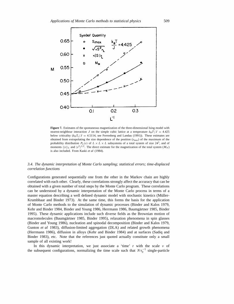
However, from equations (40) and (42) it is clear that for finiteL 〈|s|〉L is non-zero alsoin the disordered phase and thus the smooth non-singular temperature variation of〈|s|〉Lresults that is shown qualitatively in figure 6. Other estimates formspont can be extractedfrom the position of the maximums(L)max or the root-mean-square magnetization〈s2〉1/2L , butfigure 7 clearly shows that all these estimates do depend on the length scaleL, and thus anextrapolation to the thermodynamic limit,L→∞, clearly is required:
mspont= limL→∞
s(L)max= limL→∞〈|s|〉L = lim
L→∞〈s2〉1/2L . (43)
All these extrapolations are more convenient to use than the double limiting procedure thatis often used in analytical work where a symmetry-breaking field is taken to zero after thethermodynamic limit has been taken,
mspont= limH→∞
limL→∞〈s〉L,T ,H . (44)
Figure 7 illustrates the fact that one can avoid the cumbersome study of many differentsizes of (small) systems by rather analysing subsystems of one large system. As we will seebelow, doing this with the single-spin-flip algorithm described above is not really convenientbecause of ‘critical slowing down’ but this problem can be eased by using cluster algorithmsinstead (section 5.3). In any case, nearTc the size effects are clearly very pronounced and

508 K Binder
Figure 6. Schematic evolution of the order parameter distributionPL(s) from T > Tc to T < Tc
(from above to below, left-hand side) for an Ising ferromagnet, wheres is the magnetizationper site, in a box of volumeV = Ld(= L3 in d = 3 dimensions). The right-hand side showsthe corresponding temperature dependence of the mean order parameter〈|s|〉, the susceptibilitykBT χ
′ = Ld(〈s2〉−〈|s|〉2), and the reduced fourth-order cumulantUL = 1−〈s4〉/[3〈s2〉2]. Dash-dotted curves indicate the singular variation that results in the thermodynamic limit,L→∞.
thus the naive extrapolation as shown in figure 7 is not very accurate. This problem iseven more severe for the susceptibilityχ , which could be extracted from the followingextrapolations (1s is the half-width of a Gaussian peak)
kBT χ= limL→∞
(〈s2〉LLd)= limL→∞
P−2L (0)Ld/(2π)= lim
L→∞(1s)2Ld/(8 ln 2) T > Tc (45)
or
kBT χ = limL→∞
(〈s2〉L − 〈|s|〉2L)Ld = limL→∞
P−2L (s(L)max)L
d/(8/π) = limL→∞
(1s)2Ld/(8 ln 2)
T > Tc. (46)
A more efficient way of carrying out this extrapolation to the thermodynamic limit will beprovided by the finite-size scaling theory (section 4).
Applications of Monte Carlo methods to statistical physics 509
Figure 7. Estimates of the spontaneous magnetization of the three-dimensional Ising model withnearest-neighbour interactionJ on the simple cubic lattice at a temperaturekBT/J = 4.425below criticality (kBTc/J = 4.5114, see Ferrenberg and Landau (1991)). These estimates areobtained from extrapolating the size dependence of the position (smax) of the maximum of theprobability distributionPL(s) of L × L × L subsystems of a total system of size 243, and ofmoments〈|s|〉L and〈s2〉1/2. The direct estimate for the magnetization of the total system (MN )is also included. From Kaskiet al (1984).
3.4. The dynamic interpretation of Monte Carlo sampling; statistical errors; time-displacedcorrelation functions
Configurations generated sequentially one from the other in the Markov chain are highlycorrelated with each other. Clearly, these correlations strongly affect the accuracy that can beobtained with a given number of total steps by the Monte Carlo program. These correlationscan be understood by a dynamic interpretation of the Monte Carlo process in terms of amaster equation describing a well defined dynamic model with stochastic kinetics (Muller-Krumbhaar and Binder 1973). At the same time, this forms the basis for the applicationof Monte Carlo methods to the simulation of dynamic processes (Binder and Kalos 1979,Kehr and Binder 1984, Binder and Young 1986, Herrmann 1986, Baumgartner 1985, Binder1995). These dynamic applications include such diverse fields as the Brownian motion ofmacromolecules (Baumgartner 1985, Binder 1995), relaxation phenomena in spin glasses(Binder and Young 1986), nucleation and spinodal decomposition (Binder and Kalos 1979,Gunton et al 1983), diffusion-limited aggregation (DLA) and related growth phenomena(Herrmann 1986), diffusion in alloys (Kehr and Binder 1984) and at surfaces (Sadiq andBinder 1983), etc. Note that the references just quoted actually constitute only a smallsample of all existing work!
In this dynamic interpretation, we just associate a ‘time’t with the scaleν ofthe subsequent configurations, normalizing the time scale such thatNτ−1
0 single-particle

510 K Binder
transitions are attempted in unit time. This ‘time’ unit is called 1 MCS (Monte Carlo stepper particle). We consider the probabilityP(X, t) = P(Xν) that at timet a configurationXoccurs in the Monte Carlo process. This probability satisfies a Markovian master equationdP(X, t)
dt= −
∑X ′W(X →X ′)P (X, t))+
∑X ′W(X ′ →X)P (X ′, t). (47)
Equation (47) describes the balance that was already considered above (equations (31)–(34)) by a rate equation, the first sum on the right-hand side representing all processeswhere one moves away from the considered stateX (and hence its probability decreases)while the second sum contains all reverse processes (which hence lead to an increaseof the probability of findingX). In thermal equilibrium the detailed balance principle(equation (29)) ensures that these two sums always cancel and hence forP(X, t) = Peq(X)we have dP(X, t)/dt = 0, as is required. In fact,Peq(X) is the steady-state solution ofthe above master equation.
If the potential energyH(X) is finite for all configurations{X} of the system, it followsfrom the finiteness of the system that it is ergodic. However, as soon as infinite potentialsoccur (such as the excluded-volume interaction for self-avoiding walks), this is no longertrue. Even in finite systems certain configurationsX may be in disjunct ‘pockets’ of phasespace that are mutually inaccessible. There is no general rule under which conditions thisoccurs, it depends on the detailed rules for the considered moves. For example, for thealgorithms of figure 4(a) and (b) one may construct configurations of SAWs that can neitherbe reached nor left (Sokal 1995), and so the algorithms of figures 4(a) and (b) are manifestlynon-ergodic—although this does not seem to affect the accuracy in practice much (Saribanand Binder 1988).
A practically more important apparent ‘breaking of ergodicity’ occurs for systems whichare ergodic if the ‘time’ over which one averages is not long enough, i.e. less than the so-called ‘ergodic time’τe (Palmer 1982, Binder and Young 1986). This ergodicity breakingis intimately related to spontaneous symmetry breaking associated with phase transitions inthe system. In a strict sense, these phase transitions can occur only in the thermodynamiclimit N → ∞, and alsoτe diverges only forN → ∞ but can nevertheless be very largealready for finiteN . For example, for the Ising ferromagnet studied in section 3.3 we have,for T < Tc, τe ∝ PL(smax)/PL(s = 0) ∝ exp[2fint L
d−1/kBT ], wherefint is the interfacialtension between coexisting phases of opposite magnetization, as shall be discussed below.Thus lnτe ∝ N1−1/d, i.e. τe increases rapidly withN for T < Tc. Nevertheless, we assumein the following that limt→∞ P(X, t) = Peq(X), i.e. the ergodicity property can be realizedin practice.
In equation (47) we have written dP(X, t)/dt rather than1P(X, t)/1t , although thereis a discrete time increment1t = τ0/N . This step is justified since one can consider1t
as a continuous variable stochastically fluctuating with distribution(N/τ0) exp[−1tN/τ0]which has a mean value1t = τ0/N . Since the time scale on which dynamic correlationsdecay is at least of the order ofτ0, these fluctuations of the ‘time’ variable proceeding inregular steps1t = τ0/N are not important for the calculation of time-displaced correlationfunctions. The inhomogeneous updating of ‘time’, however, is crucial when one uses the‘n-fold way’ (Bortz et al 1975) or related algorithms, where particles are chosen for a moveproportional to their transition probabilityWk.
Thus we reinterpret equation (39) as a time average along the stochastic trajectory inphase space, controlled by the master equation for the system, equation (47):
A = (tM − tM0)−1∫ tM
tM0
A(t) dt (48)

Applications of Monte Carlo methods to statistical physics 511
wheretM(tM0) is the time elapsed afterM(M0) configurations have been generated
tM = Mτ0/N, τM0 = M0τ0/N. (49)
The time t is related to the labelν of the configurations ast = ντ0/N . Comparing thetime average, equation (48), with the ensemble average, equation (3) which was the startingpoint of our considerations, it is obvious that ergodicity may be a problem for importancesampling Monte Carlo, as anticipated above.
Time-displaced correlations〈A(t)B(0)〉T or A(t)B(0) are then defined as
A(t)B(0) = (tM − t − tM0)−1∫ tM−t
tM0
A(t + t ′)B(t ′) dt tM − t > tM0. (50)
Of course, one requires thattM0 can be chosen large enough so the system has alreadyrelaxed towards equilibrium during the timetM0, and then the statesX(t) included in thesampling fromtM0 to tM are already distributed according to the equilibrium distribution,P(X, t) = Peq(X), independent of time. However, it is also interesting to study theinitial non-equilibrium relaxation process by which equilibrium is approached. ThenA(t) − A depends systematically on the observation timet , and an ensemble average〈A(t)〉T − 〈A(∞)〉T is non-zero (remember that limt→∞A = 〈A〉T = 〈A(∞)〉T if thesystem is ergodic). We have defined〈A(t)〉T as
〈A(t)〉T =∑X
P(X, t)A(X) =∑X
P(X, 0)A(X, (t)). (51)
Here we have reinterpreted the ensemble average involved as an average weighted withP(X, 0) over an ensemble of initial statesX(t = 0) which then evolves as described bythe master equation, equation (47). In practice, equation (51) is realized by averaging overnrun� 1 statistically independent runs,
[A(t)]av = n−1run
nrun∑`=1
A(t, `) (52)
A(t, `) being the observableA recorded at timet in thelth run of this non-equilibrium MonteCarlo averaging. For example, these runs may differ in their random number sequence and/ortheir initial conditionX(t = 0), etc.
A discussion of the question to which type of problems such master equation descriptions(equations (47)–(52)) are applicable will be deferred to section 5. Here we are ratherinterested in applying this formalism to a discussion of statistical errors. Supposen
successive observationsAµ,µ = 1, . . . , n, of a quantityA have been recorded (n � 1).We consider the expectation value of the square of the statistical error
〈(δA)2〉 =⟨[
1
n
n∑µ=1
(Aµ − 〈A〉)]2⟩= 1
n2
n∑µ=1
〈(Aµ − 〈A〉)2〉
+ 2
n2
n∑µ1=1
n∑µ2=µ1+1
(〈Aµ1Aµ2〉 − 〈A〉2). (53)
Changing the summation indexµ2 to µ2+ µ yields
〈(δA)2〉 = 1
n
[〈A2〉 − 〈A〉2+ 2
n∑µ=1
(1− µ
n
)(〈A0Aµ〉 − 〈A〉2)
]. (54)
Now we transform to the time variablet = δtµ, δt being the time interval between twosuccessive observationsAµ, Aµ+1 (often it is more efficient to takeδt = τ0 or even 10τ0
512 K Binder
rather thanδt = 1t = τ0/N , so one need not take observations at every microstep of theprocedure). Transforming the sum to an integral yields (tn = nδt)
〈(δA)2〉 = 1
n
{〈A2〉 − 〈A〉2+ 2
δt
∫ tn
0
(1− t
tn
)[〈A(0)A(0)〉 − 〈A〉2] dt
}= 1
n(〈A2〉 − 〈A〉2)
{1+ 2
δt
∫ tn
0
(1− t
tn
)φA(t) dt
}. (55)
In the last step we have introduced the normalized relaxation function
φA(t) = [〈A(0)A(t)〉 − 〈A〉2]/[〈A2〉 − 〈A〉2] (56)
with φA(0) = 1 andφA(t →∞) = 0. We define a relaxation time from the integral
τA =∫ ∞
0φA(t) dt. (57)
For tn � τA equation (55) reduces to
〈(δA)2〉 = 1
n[〈A2〉 − 〈A〉2](1+ 2τA/δt). (58)
If δt � τA, then the second value in parentheses in equation (58) is unity to a very goodapproximation, the statistical error then is the same as for simple sampling of uncorrelateddata. In the inverse case whereδt � τA we have
〈(δA)2〉 ≈ 2τAnδt
[〈A2〉 − 〈A〉2] = 2τAtn
[〈A2〉 − 〈A〉2] (59)
which shows that the statistical error is then independent of the choice of the time intervalδt : although for a given averaging timetn a smallerδt increases the number of observations,it does not decrease the statistical error, only the ratio between the relaxation timeτA andthe observation timetn matters.
Since τA becomes very large near second-order phase transitions (‘critical slowingdown’, Hohenberg and Halperin (1977)), choice of algorithms that reduceτA becomesvery important, see section 5.3. On the other hand, careful ‘measurements’ of both〈(δA)2〉and 〈A2〉 − 〈A〉2 allow via equation (58) a straightforward estimation ofτA (Kikuchi andIto 1993).
We conclude this subsection by defining a nonlinear relaxation function
φ(nl)(t) = [〈A(t)〉T − 〈A(∞)〉T ]/[〈A(0)〉T − 〈A(∞)〉T ] (60)
and the corresponding nonlinear relaxation time
τ(nl)A =
∫ ∞0φ(nl)A (t) dt. (61)
The condition that the system is well equilibrated then simply becomes
tM0 � τ(nl)A . (62)
Equation (62) must hold for all quantitiesA, and hence one must focus on the slowestrelaxing quantity (for whichτ (nl)
A is largest) to estimatetM0 reliably. Near second-order phasetransitions, the slowest relaxing quantity usually is the order parameter of the transition andnot the internal energy. Hence the ‘rule’ published in some Monte Carlo work that theequilibration of the system is established by monitoring the time evolution of the internalenergy is a procedure that is clearly not valid in general.

Applications of Monte Carlo methods to statistical physics 513
3.5. Other ensembles of statistical physics
So far the discussion has been mostly restricted to the canonical ensemble, i.e. for an Isingmagnet, the number of lattice sites (spins)N , the temperatureT , and the external magneticfield H are the given (independent) thermodynamic variables. Of course, it is also possibleto carry out simulations in other ensembles, for example one may choose an ensemble wherethe variable thermodynamically conjugate toH , namely the magnetizationm, is given (andfixed). In fact, the spin-exchange algorithm of figure 5(b) realizes that ensemble.
In such a simulation using the (NmT ) ensemble the magnetic fieldH then is a non-trivial quantity which one may wish to calculate. This is not so straightforward as thecalculation ofm in the (NHT ) ensemble (equation (26)), because unlike the latter variableH (or other intensive thermodynamic variables, for other ensembles) cannot be directlyexpressed as function of the microscopic degrees of freedom.
For systems with discrete degrees of freedom, such as the Ising model, this problemcan be handled by the concept of ‘local states’ (Alexandrowicz 1975, 1976, Meirovitch andAlexandrowicz 1977). We use here the ‘lattice gas model’ language of the Ising problem,i.e. lattice sitesi are occupied (local densityρi = (1 − Si)/2 = 1, i.e. Si = −1) orempty (ρi = 0, Si = +1); constant magnetization corresponds then to constant density(or particle numberN , respectively) in the lattice gas, andH translates into the chemicalpotentialµ of the particles (note that theNmT ensemble of the Ising magnet correspondsto the canonicalNV T ensemble of the lattice gas, while theNHT ensemble of themagnet corresponds to the grand-canonicalµV T ensemble). Assuming that a nearest-neighbour energy−ε is won if two neighbouring sites of a square lattice are occupied, theinteraction energy of an atom can take the five valuesEα = 0, −ε, −2ε, −3ε and−4ε,respectively. We define a set of five conjugate statesα′ by removing the central atom ofeach stateα, with Eα′ = 0. If the frequencies of occurrence of the local statesα andα′ are denoted asνα and να′ , the condition of detailed balance (equation (29)) requiresthat
να/να′ = exp[(−Eα + µ)/kBT ]µ
kBT= ln(να/να′)+ Eα/kBT . (63)
To smooth out fluctuations it is advisable to averageµ over all (five) local states. Thistechnique has been used to study problems such as the excess chemical potential in a sys-tem where a droplet coexists with surrounding vapour (Furukawa and Binder 1982), forinstance.
For off-lattice systems the standard method to sample the chemical potential is the ‘testparticle insertion method’ (Widom 1963): one tries to insert a particle at a randomly chosenposition, calculates the change in energy1Et due to this test particle, and estimatesµ from
(µ− µ0)/kBT = − ln〈exp(−1Et)/kBT 〉NV T . (64)
Here µ0 is the chemical potential of an ideal gas ofN particles at temperatureT inthe same volumeV . Applications of equation (64) are ubiquitous (Allen and Tildesley1987, 1993, Allen 1996). Particular problems arise, of course, when either the systemis very dense or the particle to be inserted is a complex object (e.g. a macromolecule):then 1Et is very large and the sampling of exp(−1Et/kBT ) will not work out inpractice. For example, for the bond fluctuation model (Carmesin and Kremer 1988) offlexible polymers a chain is represented by effective monomers connected by effectivebonds on a lattice, assuming that each ‘monomer’ blocks all eight sites of an elementarycube for further occupation. For this excluded volume interaction,1Et = ∞ as soonas a monomer of the test chain overlaps with just one occupied site only. Therefore,

514 K Binder
the probability that one can insert a long chain into a dense system without overlap isextremely small—e.g. Muller and Paul (1994) estimate that for chain lengthN = 80 andvolume fractionφ = 0.5 of occupied sites this insertion probability is as small as 10−76!Various specialized techniques have been devised to overcome this problem: stepwisegrowth of macromolecules (Kumar 1994), configurational bias Monte Carlo (Frenkel 1993),thermodynamic integration (Muller and Paul 1994), ‘multicanonical’ sampling (Wilding andMuller 1994), and sampling in an ensemble with fluctuating chain lengths (Escobedo andde Pablo 1995).
For simulations of fluids in theNV T ensemble there is another intensive variable ofinterest, namely the pressurep. In systems with additive pairwise potentialsϕ(r) it isusually calculated from the Virial theorem (Hill 1956, Wood 1968)
pV/N kBT = 1− 1/(6kBT )
∫ ∞0g(r)[dϕ(r)/dr]4πr2 dr (65)
whereg(r) is the radial density pair distribution function.Equations (64) and (65) are very useful since combining them with thermodynamic
relations for the entropyS such as
T S = pV + E −Nµ (66)
one can obtain all thermodynamic potentials of interest. Alternative methods for obtainingfree energyF = E − T S or entropyS rely on ‘umbrella sampling’ (Valleau and Torrie1977) or thermodynamic integration methods, for example the relation for the specific heatCV
(∂S/∂T )V,N = CV /T (67)
is integrated as
F = E − T∫ T
0[CV (T
′)/T ′] dT ′. (68)
We emphasize that this thermodynamic integration technique is very general, it appliesto both lattice and continuum models, and is particularly convenient in conjunction withhistogram reweighting techniques (Swendsenet al 1992). Of course, any other derivativesof thermodynamical potentials can also be exploited: for example for Ising magnets therelation for the magnetizationm (equation (26))
m = −(∂F/∂H)T F(T ,H2) = F(T ,H1)−∫ H2
H1
m dH (69)
is particularly convenient (Binder 1981b). The key point of all these techniques(equations (68) and (69)) is that thermodynamic potentials such asF are completely specifiedby the independent thermodynamic variables describing the considered state, but do notdepend on the particular path on which one may think the system was brought from a‘reference state’ (for whichF and S are known) to the desired state. Consequently, onecan choose the most convenient path for the problem under consideration.
For off-lattice fluids, of course, it is very natural to consider simulations not only in thecanonical ensemble (NV T ) considered above, or in the grand-canonical ensemble (µV T ),where moves need to be considered where particles are added or removed from the system(see e.g. Levesqueet al 1984 for a discussion) but also in the constant pressure ensemble(NpT ) where the volumeV is a dynamical variable to be included in the state variableX

Applications of Monte Carlo methods to statistical physics 515
in the average, equation (28). This is recognized from noting that (Wood 1968)
〈A〉NpT =∫∞
0 dV exp[−pV/kBT ]ZN (V , T )A∫∞0 dV exp[−pV/kBT ]ZN(V, T )
=∫∞
0 dV∫
dX exp{−[pV +HN(X)]/kBT }A∫∞0 dV
∫dX exp{−[pV +HN(X)/kBT ]}
(70)
whereX is the state vector in the phase space of the canonic ensemble. Since equation (70)is formally analogous to the canonical average, equation (3), it is clear that one canstraightforwardly generalize the Monte Carlo sampling, takingX = (V , X) and modifyingequations (29) and (30) as follows:
W(X →X ′)W(X ′ →X)
= exp−[pδV + δH]/kBT . (71)
One must take into account, of course, that the different ensembles of statistical mechanicsyield equivalent results in the thermodynamic limit only, while finite-size effects are different(Hill 1963).
For simulations of solids, the anisotropy of the crystal structure may require to considerboxes with different linear dimensionsLx , Ly , Lz in different coordinate axis directions.Then it is also natural not to consider only uniform volume changesδV , but rather separatechangesδLx , δLy , and δLz, and to remember thatp as used above really is nothing butthe trace of the pressure tensor5αβ . In this context, we note that the virial relation,equation (65) generalizes as follows [rij = ri − rj ]:
5αβV/N kBT = δαβ − 1
6N kBT
⟨∑i 6=j(rij )α
∂ϕ(rij )
∂(rij )β
⟩(72)
where ϕ(rij ) is the total potential acting between particles at pointsri , rj . Followingcorresponding molecular dynamics methods (Parrinello and Rahman 1980), where both thesize and shape of the box are dynamical variables, analogous Monte Carlo methods havealso been developed (Najafabadi and Yip 1983, Ray 1993). For more details on Monte Carlomethods for off-lattice systems in various ensembles see also Frenkel and Smit (1996).
While for fluids the microcanonical (NVE) ensemble is realized, of course, if oneapplies standard molecular dynamics techniques (Ciccotti and Hoover 1986, Sprik 1996),the realization and application of the microcanonical ensemble for lattice systems such asIsing or Potts models (Potts 1952, Wu 1982) has given rise to a longstanding discussion(Creutz 1983, Bhanotet al 1984, Harris 1985, Desaiet al 1988, Litz et al 1991, Huller1992, 1994, Gerling and Huller 1993, Ray 1991, Hammrich 1993, Promberger and Huller1995, Lee 1995, Grosset al 1996). Some researchers maintain that this ensemble haspractical advantages, particularly for the study of first-order phase transitions (Huller 1992,1994, Grosset al 1996), even in comparison with the popular ‘multicanonical’ method(Berg and Neuhaus 1992, Berg 1992), see section 5.3.
At this point we mention that it is sometimes convenient to define artificial‘ensembles’ that are not found in the standard text books of statistical mechanics, butcan also be translated into an importance sampling Monte Carlo method: the ‘Gaussianensemble’ of Challa and Hetherington (1988) in a sense ‘interpolates’ between thecanonical and microcanonical ensemble; and particularly important is the ‘Gibbs ensemble’(Panagiotopoulos 1987, 1992, 1994, Smit 1993, Allen 1996) for the study of gas–liquidcoexistence. There one considers two systems at the same temperature with particle numbersN1 , N2, and volumesV1, V2 such thatV1 + V2 = Vtot = constant,N1 + N2 = constant,

516 K Binder
but allows exchange of both particles and volume between the two boxes. For example, bya choice of initial condition, one can ensure (at temperatures sufficiently below the criticalpoint) that one system equilibrates at the density of the gas and the other at the liquid density.The chemical potential adjusts itself to its value at the coexistence curveµcoex automatically(in the limit Vtot→∞). This method outside of the critical region works rather well alreadyfor rather small sizes of the total volumeVtot, and hence has found widespread practicalapplication (Allen 1996, Frenkel and Smit 1996). However, once more we add the warningthat finite-size effects differ in different ensembles and need careful consideration (see e.g.Mon and Binder 1992, Recht and Panagiotopoulos 1993, Bruce 1997).
4. Finite-size effects
Simulations deal with a much smaller number of degrees of freedom (typically the particlenumberN is in the range 102 6 N 6 106) than typical experiments (N ≈ 1022). Finite-size effects thus can be a serious limitation, particularly near phase transitions where sucheffects are large. On the other hand, unlike experiment one can easily vary the system lineardimension over a wide range as a control parameter (avoiding unwanted surface effects byperiodic boundary conditions), and apply the corresponding finite-size scaling theory (Fisher1971, Barber 1983, Binder 1987a, 1992a, Privman 1990, Dunweg 1996) as a powerful toolof analysis for the simulation data. In this spirit, this section will provide a brief introductionto the main ideas of the subject.
4.1. The percolation transition and the geometrical interpretation of finite-size scaling
Consider an infinite lattice (d-dimensional cubic lattice of volumeLd , lattice spacing beingunity, for L → ∞) where each site is randomly occupied (with probabilityp) or empty(probability 1− p), and define ‘clusters’ of neighbouring occupied sites (Stauffer andAharony 1992). There exists a critical valuepc such that forp < pc there exist onlyclusters of finite ‘size’ (= number of sites belonging to the cluster,` = 1, 2, 3, . . .) on thelattice, while forp > pc an infinite cluster has formed that spans from one boundary of thelattice to the opposite one. The probability that an occupied site is part of the percolatingcluster is called the percolation probabilityP∞(p), while a percolation susceptibilityχ(p)is defined in terms of the concentrationsn`(p) of clusters containing occupied sites,
χ(p) =∞∑`=1
′`2n`(p)/p. (73)
Here the prime means that the largest cluster (forp > pc this is the percolating infinitecluster) is omitted from the summation. Bothχ(p) and the percolation order parameterP∞(p) exhibit critical singularities as|p − pc| → 0, with critical exponentsβp, γp andamplitudesBp, 0±p ,
P∞(p) = Bp(p/pc− 1)βp p > pc (74)
while per definitionP∞(p) = 0 for p < pc, and
χ(p) ={0+p (1− p/pc)
−γp p < pc
0−p (p/pc− 1)−γp p > pc.(75)
In a finite lattice, χ(p) cannot diverge but reaches a maximum of finite height only:equation (73) then is a finite sum over clusters of finite ‘mass’`, infinitely large clusters

Applications of Monte Carlo methods to statistical physics 517
would not fit on a finite lattice. Similarly, the percolation probabilityP∞(p) does notvanish at anyp > 0, but must attain small non-zero values as soon asp > 0: percolationonly requires a string ofL occupied sites running through the system, which occurs withprobability pL = exp(L`np) → 0 asp → 0. Thus in a finite lattice the singularitiesdescribed by equations (74) and (75) are smoothed out: this rounding of the transition isqualitatively obvious geometrically.
For a quantitative description of this finite-size rounding, we need the detailed propertiesof the percolation clusters nearpc (Stauffer 1979). Calling the ‘mass’ of a cluster, themass distributionn`(p) satisfies a scaling property forL→∞,
n`(p) = `−τ n{`σ (1− p/pc)} p→ pc, `→∞ (76)
n(Z) being a scaling function, and the exponentsτ, σ related toβp, γp,
τ = 2+ βp/(γp + βp) σ = 1/(γp + βp). (77)
The large clusters nearpc actually are ‘fractals’ (Mandelbrot 1982, Feder 1988), i.e. theirmass` and radiusr` are not related via space dimensionalityd but via a smaller ‘fractaldimensionality’df ,
r` = r`1/df `→∞, p = pc. (78)
Noting that in a finite subsystem of linear dimensionLs a percolating cluster hasr` = Ls,we find a relation betweendf and τ , since the probabilityP (Ls)
s (pc) that such a clusteroccurs that spans the subsystem is of order unity,
P (Ls)s (pc) ≈ Lds
∫ ∞r`=Ls
n`(pc) d` ≈ Lds n(0)∫ ∞(Ls/r)
df
`−τ d` ≈ 1. (79)
In a finite subsystem, percolation can occur via any cluster of linear dimensionr` = Ls
or larger, but these possibilities are mutually exclusive in this subsystem, and thus theirprobabilities simply add up. For large,
∑` can be replaced by
∫d`, and using equation (76)
we arrive at equation (79), which yields further
Ld+df(1−τ)s ∝ 1 df = d/(τ − 1) = d − βp/νp. (80)
Since the first equation of equation (80) must hold for anyLs, the second equation follows,using also equation (77) and the ‘hyperscaling relation’ (Fisher 1974)
dνp = γp + 2βp. (81)
In equations (80) and (81),νp is the critical exponent of the correlation lengthξp whichdescribes the decay of the pair connectedness function,
ξp ∝ |p − pc|−νp . (82)
The number of sites in a cluster that spans the distanceLs is simply (equations (78) and(80))
`Ls = (Ls/r)df ∝ Ld−βp/νps . (83)
Since the subsystem containsLds sites, the fraction of its sites belonging to such a spanningcluster are of the order of
P (L)∞ (pc) = L−d`L ∝ L−βp/νp . (84)
In equation (84), we have omitted the index s (for ‘subsystem’) fromLs, since the resultapplies to a finite system with periodic boundary conditions as well. Relations such asequation (78) also hold in finite systems essentially, as long asr` < L: the finite size yieldsa cut-off to the distributionn`(p) at the value L ∝ Ldf corresponding tor` = L.
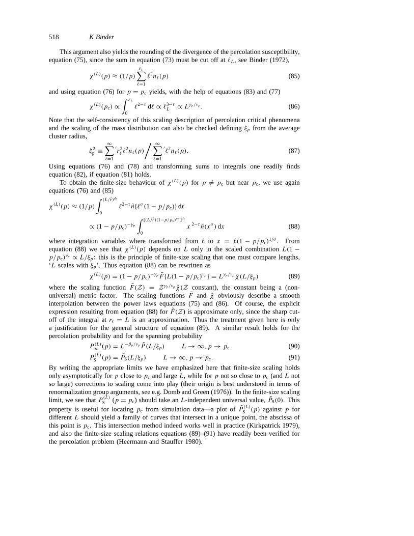
518 K Binder
This argument also yields the rounding of the divergence of the percolation susceptibility,equation (75), since the sum in equation (73) must be cut off at`L, see Binder (1972),
χ(L)(p) ≈ (1/p)`L∑`=1
`2n`(p) (85)
and using equation (76) forp = pc yields, with the help of equations (83) and (77)
χ(L)(pc) ∝∫ `L
0`2−τ d` ∝ `3−τ
L ∝ Lγp/νp . (86)
Note that the self-consistency of this scaling description of percolation critical phenomenaand the scaling of the mass distribution can also be checked definingξp from the averagecluster radius,
ξ2p ≡
∞∑`=1
′r2` `
2n`(p)
/ ∞∑`=1
′`2n`(p). (87)
Using equations (76) and (78) and transforming sums to integrals one readily findsequation (82), if equation (81) holds.
To obtain the finite-size behaviour ofχ(L)(p) for p 6= pc but nearpc, we use againequations (76) and (85)
χ(L)(p) ≈ (1/p)∫ (L/r)df
0`2−τ n{`σ (1− p/pc)} d`
∝ (1− p/pc)−γp
∫ [(L/r)(1−p/pc)νp ]df
0x 2−τ n(xσ ) dx (88)
where integration variables where transformed from` to x = `(1 − p/pc)1/σ . From
equation (88) we see thatχ(L)(p) depends onL only in the scaled combinationL(1 −p/pc)
νp ∝ L/ξp: this is the principle of finite-size scaling that one must compare lengths,‘L scales withξp ’. Thus equation (88) can be rewritten as
χ(L)(p) = (1− p/pc)−γp F {L(1− p/pc)
νp } = Lγp/νp χ(L/ξp) (89)
where the scaling functionF (Z) = Zγp/νp χ(Z constant), the constant being a (non-universal) metric factor. The scaling functionsF and χ obviously describe a smoothinterpolation between the power laws equations (75) and (86). Of course, the explicitexpression resulting from equation (88) forF (Z) is approximate only, since the sharp cut-off of the integral atr` = L is an approximation. Thus the treatment given here is onlya justification for the general structure of equation (89). A similar result holds for thepercolation probability and for the spanning probability
P (L)∞ (p) = L−βp/νp P (L/ξp) L→∞, p→ pc (90)
P(L)
S (p) = PS(L/ξp) L→∞, p→ pc. (91)
By writing the appropriate limits we have emphasized here that finite-size scaling holdsonly asymptotically forp close topc and largeL, while for p not so close topc (andL notso large) corrections to scaling come into play (their origin is best understood in terms ofrenormalization group arguments, see e.g. Domb and Green (1976)). In the finite-size scalinglimit, we see thatP (L)S (p = pc) should take anL-independent universal value,PS(0). Thisproperty is useful for locatingpc from simulation data—a plot ofP (L)S (p) againstp fordifferentL should yield a family of curves that intersect in a unique point, the abscissa ofthis point ispc. This intersection method indeed works well in practice (Kirkpatrick 1979),and also the finite-size scaling relations equations (89)–(91) have readily been verified forthe percolation problem (Heermann and Stauffer 1980).

Applications of Monte Carlo methods to statistical physics 519
4.2. Broken symmetry and finite-size effects at critical points
We now discuss thermally-driven phase transitions where the state of the system changesfrom the disordered phase at high temperatures to a spontaneously ordered state at atemperatureT below the critical temperatureTc of a second-order transition, using theIsing ferromagnet as a prototype example. The low-temperature phase is a state with non-zero spontaneous magnetization±mspont for zero applied fieldH = 0 (cf figures 6 and7).
As described already in section 3.2, there is always a non-zero probability in a finitesystem to ‘move’ from the state near+mspont to the state with−mspont or vice versa, andthus 〈m〉 ≡ 0 for H = 0. The standard recipe (also useful for vector order parameters,as they occur forXY or Heisenberg models, equations (35) and (36)) is to record theroot-mean-square order parameter (Binder 1972)
mrms(T ) =√〈m2〉T =
⟨( N∑i=1
Si/N
)2⟩1/2T
= 1
N
( N∑i,j=1
〈SiSj 〉T)1/2
. (92)
Now the correlation function (r = ri − rj is the distance between sitesi, j )
G(r, T ) ≡ 〈SiSj 〉T (93)
satisfies a power-law decay forT = Tc (Fisher 1974)
G(r, Tc) = Gr−(d−2+η) r →∞ (94)
with η the corresponding exponent andG the critical amplitude. We can approximatelyevaluate equation (92) forT = Tc, using equations (93) and (94) and replacing the sum
∑by an integral over distances from 0 toL/2 (N = Ld ), to obtain
N∑i=1
〈SiSj 〉Tc ∝∫ L/2
0rd−1 drG(r, Tc) ∝ L2−η (95)
and hence (Muller-Krumbhaar and Binder 1972)
m(L)rms(Tc) ∝ (L2−d−η)1/2 ∝ L−β/ν (96)
using scaling relations (Fisher 1974) 2− η = γ /ν, d = (2β + γ )/ν. Also the fluctuationrelation for the susceptibility (cf equation (45)) yields (rememberH = 0)
kBT χ(T ) = 1
N
∑i,j
〈SiSj 〉T ∝T=Tc
L2−η = Lγ/ν (97)
using again equation (95). Equations (96) and (97) are exactly analogous to the resultsequations (84) and (86) for the percolation problem.
Of course, the analogy between the finite-size results for the Ising model and for randompercolation is no surprise at all: the mapping proved by Fortuin and Kasteleyn (1972)between bond percolation and the limitq → 1 of theq-state Potts model (Potts 1953, Wu1982) provides a description of the thermal order–disorder transition of the Ising model (andrelated spin models) as a percolation of ‘physical clusters’ (Coniglio and Klein 1980, Hu1984, Swendsen and Wang 1987). Any state of the Ising lattice can be described in termsof ‘geometrical clusters’ of, say, ‘down spins’ in a surrounding background of ‘up spins’(Fisher 1967, Binder 1976). However, throughout the paramagnetic phase we encounter apercolation transition of these ‘geometrical clusters’ when we vary the magnetic fieldH
from strongly positive to negative values. Rather one has to distinguish between ‘active’and ‘inactive’ bonds in a geometrical cluster. The probabilityp for a bond to be active is
p = 1− exp(−2J/kBT ) (98)

520 K Binder
and only spins connected by ‘active bonds’ form a ‘physical cluster’ (Coniglio and Klein1980). This rule can be proven (Fortuin and Kasteleyn 1972) by deriving a percolationrepresentation of the Potts model partition functionZPotts, Jp being the interaction constantof the Potts Hamiltonian (note thatHPotts reduces toHIsing for q = 2, choosingJp = 2J )
HPotts= −Jp
∑〈i,j〉
δσiσj σi = 1, 2, . . . , q (99)
ZPotts= Tr{σi } exp(−HPotts/kBT ) =∑
pNb(1− p)NmqNc (100)
whereNb is the number of bonds,Nm is the number of missing bonds, andNc is thenumber of clusters in a given bond configuration. The sum in equation (100) is over allbond configurations.
For expressing the variables of interest, we now need two ‘cluster coordinates’ (Binder1976), the cluster magnetizationmcl = ±` (the sign gives the orientation of the spins insidethe cluster, which we label as cl), and the number of active bonds in the cluster, whichwe denote asuclp. Denoting the number of clusters per lattice sites with these propertiesas p(mcl, ucl), magnetization and energy per spin atH = 0 are written, for a lattice ofcoordination numberz,
m =∑mcl
mclP(mcl) P (mcl) ≡∑ucl
p(mcl, ucl) (101)
E = 〈HIsing〉/N = − z2J
(∑mcl
∑ucl
uclp(mcl, ucl)− 1
)= − z
2J (p〈Nb〉/N − 1) (102)
remembering thatNb is the total number of (active) bonds in a configuration. Also thethermal averages of fluctuations can be expressed in terms of suitable properties of theclusters; for example, the specific heat per lattice site becomes
C = ∂E/∂T = [1/(NkBT2)](〈H2
Ising〉 − 〈HIsing〉2)= 1
4z2J 2/(NkBT
2p2){〈N2b 〉 − 〈Nb〉2− (1− p)〈Nb〉}. (103)
Splitting off from P(mcl) the contribution of the largest cluster in the system, which wedenote asm∞cl ,
P(mcl) ≡ p′(mcl)+ 1
Nδmcl,m
∞cl
(104)
the absolute value of the magnetization is (D’Onorio De Meoet al 1990)
〈|m|〉 =⟨∣∣∣∣m∞cl
N+∑mcl
mclp′(mcl)
∣∣∣∣⟩. (105)
While the susceptibility forT > Tc is just the analogue of the percolation susceptibility,equation (73),
kBT χ = kBT (∂〈m〉/∂H)T,H=0 =∑mcl
m2clP(mcl) =
∑`
`2n` (106)
sinceP(mcl) + P(−mcl) = n`, for T < Tc one must single out the contribution from thelargest cluster (that becomes the percolating cluster forN → ∞) to obtain (D’Onorio DeMeo et al 1990)
kBT χ′ = N(〈m2〉 − 〈|m|〉2) =
∑`
′`2n` +N(〈P 2
∞〉 − 〈|m|〉2)
≈∑`
′`2n` +N(〈P 2
∞〉 − 〈P∞〉2). (107)

Applications of Monte Carlo methods to statistical physics 521
The simple physical interpretation of equation (107) is, of course, that belowTc theresponse function picks up contributions both from all finite clusters (the term
∑′` `
2n`,only considered in the percolation problem) and from the fluctuations in size of the largest(percolating) cluster. It turns out that estimatingχ, χ ′ from these relations in terms ofclusters is advantageous in comparison with the fluctuaton relations expressing them bymagnetization fluctuations, since equations (106) and (107) exploit the fact that there areno correlations between different clusters: thus the statistical noise is less, the right-handsides of equations (106) and (107) are ‘improved estimators’. Similar ‘improved estimators’can also be introduced for other quantities, for example the pair correlation function (Wolff1989a, Janke 1994), wavevector-dependent susceptibility, and fourth-order cumulant (Bakerand Kawashima 1995, 1996). Since Monte Carlo ‘cluster algorithms’ (Swendsen andWang 1987, Swendsenet al 1992, Wolff 1988a, b, 1989a, b, c, 1992, Edwards and Sokal1989, Hu and Mak 1989, Wanget al 1989, Kandelet al 1990, Hasenbusch and Meyer1991) are attractive because they reduce ‘critical slowing down’(Li and Sokal 1989, 1991,Wang 1991, Heermann and Burkitt 1990, Tamayoet al 1990, Wolff 1992), one can applyequations (101)–(107) at no extra computational cost. Figure 8 shows an example for thed = 2 Ising square lattice. It is clearly seen that for finite systems the percolation probabilityP∞ = 〈|m∞cl |〉/N is always smaller than〈|m|〉, as expected from equation (105), althoughin the limit N → ∞ both quantities converge to the spontaneous magnetization. Notethat even forN → ∞ the termN(〈P 2
∞〉 − 〈P∞〉2) must not be neglected inkBT χ′ in
comparison to∑′
` `2n` for T < Tc, although it is negligible forT > Tc (one can show that
N(〈P 2∞〉 − 〈P∞〉2) ∝ L−d log2L for L → ∞ and T > Tc, see Margolina and Heermann
(1984)).While in the percolation problem one hence can use the same expression, equation (73),
to obtain the percolation susceptibility forp < pc and for p > pc, this is not true forthe phase transition of the Ising model, equations (106) and (107) differ from each othersignificantly.
This difference, of course, is intimately linked to the occurrence of spontaneoussymmetry breaking in the Ising model, already alluded to in figure 6 and equations (45)and (46). As illustrated in figure 9, the fluctuation relation for the susceptibilitykBT χ =Ld(〈m〉2−〈m〉2) = Ld〈m2〉 (for zero fieldH = 0) smoothly converges to the correct answerfor T > Tc , but for T < Tc it converges tokBT χ ≈ Ld〈|m|〉2 asL→∞, measuring thefluctuations between the two phases with opposite magnetization, rather than the fluctuationsin a pure phase. On the other hand,kBT χ
′ as defined by equation (107) forT > Tc does notconverge to the right answer either: as one can easily work out from a Gaussian distribution(Binder and Heermann 1988),χ ′ = χ(1− 2/π) for L → ∞. Thusχ ′ diverges with thesame critical exponent asχ does, but the prefactor (the critical amplitude) is reduced by afactor 1− 2/π .
The fact that the spontaneous symmetry breaking in phase transitions requires the useof different fluctuation formulae on both sides of the transition is sometimes ignored in theliterature, which hence leads to confusion: for a finite system in zero field,〈m〉2 and henceLd(〈m2〉−〈m〉2) is not a useful quantity, if a single spin-flip algorithm is used. ForT � Tc,the observation timetobs of the simulation will be much smaller than the ‘ergodic time’ (τe
needed to move from one peak ofPL(m) in the lower part of figure 6 to the other one, andhence〈m〉2 ≈ 〈|m|〉2, and thenLd(〈m2〉 − 〈m〉2) will coincide with kBT χ ! For T > Tc,tobs will exceed τe by orders of magnitude, and then〈m〉2 ≈ 0, i.e. one obtainskBT χ
(figure 9). However, in the region wheretobs andτe are of the same order of magnitude, themagnetization will jump between the two peaks ofPL(m) only very infrequently, and thenone obtains rather erratic results ofLd(〈m2〉 − 〈m〉2), since〈m〉 is not well defined here.

522 K Binder
Figure 8. (a) Magnetization (full curves) and percolation probability (broken curves) for thed = 2 nearest-neighbour Ising ferromagnet plotted against reduced temperature for three systemsizes as indicated. Periodic boundary conditions were used throughout, and all data weregenerated with the algorithm of Swendsen and Wang (1987). From D’Onorio de Meoet al(1990). (b) Normalized fluctuation of the largest cluster,N(〈P 2∞〉 − 〈P∞〉2), full curves, andsecond moment of the cluster size distribution,
∑′`2n`, broken curves, plotted againstT/Tc,
for the same model as in (a). From D’Onorio De Meoet al (1990).
From the percolation interpretation of the transition, it is clear that finite-size scalingexpressions analogous to equations (89)–(91) hold for〈|m|〉, χ, χ ′ and a further useful

Applications of Monte Carlo methods to statistical physics 523
Figure 9. Schematic temperature variation of the normalized susceptibilitieskBT χ(L, T ) =Ld(〈m2〉 − 〈m〉2) = Ld 〈m2〉 and kBT χ
′(L, T ) = Ld(〈m2〉 − 〈|m|〉2). The dash-dotted curveillustrates the observed behaviour forLd(〈m2〉 − 〈m〉2) in simulations with the single spin-flip algorithm: for observation timestobs of the order of the equilibration timeτe (noteln τe ∝ Ld−1fint(T ), wherefint(T ) is the interfacial tension) one finds an interpolation betweenkBT χ (at high temperatures wheretobs� τe) andkBT χ
′ (at low temperatures wheretobs� τe).For smallL and largetobs this ‘transition’ may be rather far belowTc and should not beconfused with the phase transition. ForL→∞, of course, this temperature region between thetemperature wheretobs= τe andT = Tc shrinks and ultimately vanishes: symmetry breaking atTc simply appears via ‘ergodicity breaking’. From Binder and Heermann (1988).
quantity, the normalized fourth-order cumulantUL (Binder 1981a) of the distributionPL(m),
UL = 1− 〈m4〉/(3〈m2〉2). (108)
In terms ofε = T/Tc − 1 we have, withM, ˜M, χ, ˜χ, χ ′, ˜χ ′, U , ˜U being suitable scalingfunctions
〈|m|〉 = L−β/νM(L/ξ) = L−β/ν ˜M(εL1/ν) (109)
kBT χ = Lγ/νχ(L/ξ) = Lγ/ν ˜χ(εL1/ν) (110)
kBT χ′ = Lγ/νχ ′(L/ξ) = Lγ/ν ˜χ ′(εL1/ν) (111)
UL = U (L/ξ) = ˜U(εL1/ν). (112)
Figure 10 shows an example where the scaling ofkBT χ′ (equation (111)) is tested. It
must be emphasized that all these scaling relations are only supposed to hold in the limitsL → ∞, ε → 0 (keepingεL1/ν or L/ξ fixed). While it is gratifying to note that in theexample shown in figure 10 rather smallL (such asL = 20 in d = 2) already satisfy thisfinite-size scaling hypothesis, one cannot imply that this ‘data collapsing’ on the scalingfunction will work for rather smallL in general (in fact, when one has crossover from

524 K Binder
Figure 10. Finite-size scaling plot ofkBT χ′L−γ /ν against|ε|L1/ν , where ε = T/Tc − 1,
for the two-dimensional Ising model with nearest-neighbour ferromagnetic interaction at thesquare lattice. The exactly known value ofTc (Onsager 1944) and of the critical exponents(ν = 1, γ = 7/4, see e.g. Fisher (1974)) are used. Three different lattice sizes are included, asindicated in the figure. The upper branch of the scaling function refers toT < Tc, the lowerbranch toT > Tc. From D’Onorio De Meoet al (1990).
one universality class to another, e.g. from the Ising class to mean-field behaviour (Monand Binder 1993, Deutsch and Binder 1993a, Binderet al 1996, Luijtenet al 1996) finite-size scaling only works forL � ξcross, with ξcross a length characterizing this crossover(Binder and Deutsch 1992)). For smallL one thus must expect corrections to finite-sizescaling. Thus methods where one ignores such corrections and tries to estimate bothTc andthe exponents 1/ν, γ /ν (and/orβ/ν) from a simultaneous fit to a scaling function (‘datacollapsing’, see e.g. Binder (1974), Landau (1976a, b) and Binder and Landau (1980) forsome well known examples), may suffer from systematic errors. This criticism also appliesto recent claims (Kim 1993, Brown and Cittan 1996) that high precision can be gained byextrapolation from small lattices, as pointed out by Patrasciou and Seiler (1994) and Holmand Janke (1997).
In an attempt to estimateTc unbiased from estimates of critical exponents, Binder(1981a) suggested the plotting ofUL againstT for various choices ofL, since in the limitwhere finite-size scaling holds these curves should intersect in a common intersection pointU (0) at Tc, and moreoverU (0) is universal (though dependent on the type of boundaryconditions). In fact, other dimensionless moments of the order parameter distribution maybe used in the same way, for example〈m2〉/〈|m|〉2 (Deutsch and Binder 1992). Figure 11presents a typical example of the accuracy that is reached by such techniques, namely about0.3%, even for rather complicated models such as polymer mixtures. Of course, a closeinspection of figure 11 shows that the three curves do not intersect precisely in a point, butthere is rather a small temperature interval over which these intersections are spread out. Tosome extent this spread is due to statistical errors, to some extent to corrections to scaling.

Applications of Monte Carlo methods to statistical physics 525
Figure 11. Plot of 〈m2〉/〈|m|〉2 against reduced temperature, for a lattice model of a symmetricalpolymer mixture (using the bond fluctuation model with chain lengthsNA = NB = N = 128 atvolume fractionφ = 0.5 of occupied sites, and a square well interactionε(= εAB = −εAA /2=−εBB/2) of range
√6). Three lattice sizes are shown as indicated, and a semi-grand canonical
ensemble is used (allowing attempted moves while chains change their identity, A⇔ B, atfixed configuration, in addition to local hopping moves that relax the chain configurations).Smooth curves are based on multihistogram extrapolations (Ferrenberg and Swendsen 1989).From Deutsch and Binder (1992).
If Tc is known the exponentβ/ν can be estimated from a log–log plot of〈|m|〉 againstL at Tc, using equation (109). The exponentβ/ν can be estimated both from log–log plotsof kBT χ or kBT χ
′ againstL at Tc, or alternatively from a log–log plot of the maximumvaluekBT χmax againstL (this has the advantage that a possible inaccuracy ofTc does notmatter). From equation (111) we realize that the location of this maximum can be used toestimate the exponent 1/ν, since the maximum occurs at some fixed valuexm = εmL
1/ν ofthe scaling function (εm ≡ Tm/Tc− 1, Tm(L) being the temperature of the maximum)
Tm(L)/Tc− 1= xmL1/ν L→∞. (113)
Alternatively, one can use the slope ofUL− ˜U(0) ∝ εL1/ν for smallεL1/ν (equation (112)).In addition, one can use the position of the maximum of the slope ofUL againstT , thespecific heat maximum, the maximum of the temperature derivative of〈|m|〉 or 〈m2〉 etc(Ferrenberg and Landau 1991). One can also use such quantities to try to obtain both 1/ν
andTc from a simultaneous fit.In principle, for obtaining very precise estimates the effect of correction terms must be
considered, for example, atTc we expect instead of equation (97)
kBTcχ(Tc) = Lγ/νχ(0)(1+ χcorrL−xcorr + · · ·) (114)
χcorr being another amplitude factor andxcorr the leading correction exponent. Such acorrection shows up as a mild curvature on the log–log plot, and is hence easily missed. Inorder to take this correction into account, it is advisable to consider pairs of sizes (L, bL)for scale factorsb > 1, and study the ratio (Binder 1981a)
ln[χ(bL, Tc)/χ(L, Tc)]
ln b= γ
ν− χ
corrL−xcorr
ln b(1− b−xcorr)+ · · · . (115)

526 K Binder
Thus the recipe is to plot the left-hand side of equation (115) against(ln b)−1: for eachchoice ofL one should obtain a curve which will extrapolate linearly to the same value (γ /ν)as(ln b)−1→ 0. This method was also tried with some success for non-trivial cases such astwo-dimensional Ising antiferromagnets with competing next-nearest-neighbour interactions(Landau and Binder 1985), which belong to the universality class of theXY model withcubic anisotropy and have non-universal exponents (Krinsky and Mukamel 1977).
Comparing equations (109) and (110) and using the fact that〈m2〉Tc ∝ L−2β/ν weimmediately see that the fluctuation relationkBT χ = Ld〈m2〉 yields the hyperscalingrelation (Fisher 1974),γ /ν = d − 2β/ν: finite-size scaling as written in equations (109)–(112) implies hyperscaling (Binder 1981a, Brezin 1982). However, there do indeed occursituations where hyperscaling does not hold, and then a generalization of finite-size scalingis necessary. A well known example are systems at dimensionalitiesd above the marginaldimensiond∗ above which mean-field theory of critical behaviour starts to become valid(Fisher 1974). For Ising systems (as well as for then-vector model)d∗ = 4, and clearlythe mean-field exponents(γMF = 1, νMF = 1/2, βMF = 1/2) do not satisfy hyperscaling ford > 4. In the general case (including anisotropic system shapes (Binder and Wang 1989),free surfaces, etc) several characteristic lengths come into play, and the behaviour can bevery complicated (Brezin and Zinn-Justin 1985). However, for systems with aLd geometryand fully periodic boundary conditions a simple modified form of finite-size scaling holds(Binder et al 1985), the correlation lengthξ being replaced by a ‘thermodynamic length’`T (Binder 1985) defined by
`dT = kBT χ′m−2 ∝ (1− T/Tc)
−(γ+2β) = (1− T/Tc)−2 (116)
where, in the last step, mean-field exponents were used. Equation (116) can be motivatedby noting that forT < Tc and largeL the order parameter distributionpL(m) can beapproximated as a sum of two Gaussians centred at the spontaneous magnetization (cffigure 6), forH = 0,
pL(m) ∝ exp
[−(m−mspont)2Ld
2kBT χ ′
]+ exp
[−(m+mspont)2Ld
2kBT χ ′
](117a)
and the arguments of the exponentials can be scaled as follows:
(m±mspont)2Ld
2kBT χ ′= (m/mspont± 1)2
2
Ld
kBT χ ′m2spont
= (m/mspont± 1)2
2
(L
`T
)d. (117b)
While some consequences of this mean-field finite-size scaling initially seemed to be indisagreement with simulations on five-dimensional Ising models (Binder 1985, Rickwardtet al 1994), recently the source of the difficulty has been traced down to corrections toscaling (Mon 1996, Luijten 1997, Parisi and Ruiz-Lorenzo 1996).
Another violation of hyperscaling is believed to occur in random-field Ising models(RFIM) (for reviews, see e.g. Imry 1984, Nattermann and Villain 1988, Rieger 1995) andrandom-field Potts models (RFPM) (Eichhorn and Binder 1995, 1996). If these systemshave a second-order transition from the ferromagnetic to the paramagnetic state at all, theexponents are believed to satisfy a modified hyperscaling law (e.g. Schwartz 1991)
γ + 2β = (d − θ)ν θ = 2− η. (118)
In spite of equation (118) the standard finite-size scaling relations equations (109)–(111)still hold, notwithstanding the fact that thenLd〈m2〉Tc ∝ Ld−2β/ν : in this case〈m〉2 isnon-zero, due to the excess of random field of one particular sign in any finite sample, andone must distinguish between the ‘connected’ susceptibility (kBT χ = Ld([〈m2〉 − 〈m〉2])av

Applications of Monte Carlo methods to statistical physics 527
Figure 12. Plot of the cumulantUL(Tc) for the two-dimensional Ising transition in thin filmsof thicknessD with competing surface fieldsH1 = −HD = 0.55J against the crossoverscaling variableξcross/L. Here ξcross= exp(κcD/2), whereκ−1
c = ξb(1+ ω/2), ξb being thetrue correlation length in the bulk, andω(≈ 0.86) is the universal amplitude associated withinterfacial stiffness. The arrow on the ordinate shows the universal value of thed = 2 Isinguniversality class,U∗ = 0.615. From Binderet al (1996).
∝T=Tc Lγ/ν) and the ‘disconnected susceptibility’χdis ≡ Ld [〈m〉2]av, [. . .]av meaning a
‘quenched average’ (Binder and Young 1986) over the random-field configurations. Whileχdis(T = Tc) ∝ Lγ/ν and γ satisfies hyperscalingγ + 2β = dν), in the connectedsusceptibility a smaller exponent(γ = γ /2) results, because the two leading terms canceleach other, and only a subleading correction remains. This is only possible because in thescaling limit of the distributionPL(m) the position of the peaks scale with a less negativeexponent(−β/ν) than the width((γ /ν−d)/2). Since forL→∞ at Tc, PL(m) becomes asum of delta functions, the cumulant intersection method is less useful:UL (equation (108))tends to 2/3 atTc as in the low-temperature phase, and there is no well defined intersectionpoint (Eichhorn and Binder 1996). In contrast, for other random systems such as spin glasses(Binder and Young 1986) or Potts glasses (Binder and Reger 1992) the cumulant intersectionmethod has been the most useful method to check for the existence of static phase transitionsin thermal equilibrium (Young 1996), since the lack of cumulant intersections can be taken asevidence that the system is at or below its lower critical dimension for a spin glass transition.
Non-trivial extensions of finite-size scaling are necessary to deal with tricriticalphenomena (Wilding and Nielaba 1996) and anisotropic critical phenomena, where thecorrelation length diverges with a (larger) exponentν‖ in a distinct direction(ξ‖ ∝|1− T/Tc|−ν‖) than in the perpendicular direction(s) (ξ⊥ ∝ |1− T/Tc|−ν⊥ , ν⊥ < ν‖). Thelatter case occurs at uniaxial Lifshitz points as they occur for the anisotropic next-nearest-neighbour Ising (ANNNI) model (Selke 1988), for critical wetting transitions (Dietrich1988), and—last but not least—for driven systems far from equilibrium, such as the chargedlattice gas under the action of an electrical field (Schmittmann and Zia 1995).

528 K Binder
Denoting the linear dimensions of the system in the parallel and perpendicular directionsasL or L⊥, respectively, an extension of finite-size scaling to this case (Binder and Wang1989) showed that in addition to the variableεL
1/ν‖‖ (cf equations (109)–(112)) one needs
a second variable, a generalized aspect ratioLν⊥/ν‖‖ /L⊥ (this factor reduces to the standard
aspect ratioL‖/L⊥ for isotropic critical phenomena, of course, needed to describe shapeeffects near criticality, see Binder and Wang (1989) and Albanoet al (1989a)). After along controversy about the critical behaviour of the two-dimensional driven lattice gas afinite-size scaling study along these lines (Wang 1996) finally obtained consistency withthe field-theoretic predictions. We return now to ‘simple’ critical phenomena such as theliquid–gas transition but consider systems that lack the particular particle–hole symmetryof the Ising lattice gas model, for example off-lattice fluids. Not only has then the criticalpoint to be searched for in a two-dimensional parameter space (temperatureT and thechemical potentialµ, for instance), but there are also rather strong corrections to scalinginduced by a coupling between order parameter density and energy density fluctuations(Wilding and Bruce 1992, Wilding 1993, 1995, Wilding and Muller 1995). The critical partof the energy density scales withL asL−(1−α)/ν whereα is the specific heat exponent (e.g.Milchev et al 1986), and this needs to be disentangled from the order parameter that scalesasL−β/ν . Wilding and Bruce (1992) and Wilding (1993, 1995) solved this problem by alinear transformation from the densityρ and energy densityu to the appropriate ‘scalingfields’. Using this technique in the context of grand-canonical simulations of simple fluids,a satisfactory analysis of their critical region became feasible (Wilding 1995, 1996). Also asuccessful extension of this concept to asymmetrical polymer mixtures (Muller and Wilding1995) was given. For critical properties, these techniques are superior to both the ‘Gibbsensemble’ method (Panagiotopoulos 1987, 1992, 1994, Smit 1993, Allen 1996) and standardfinite-size scaling applied to subboxes (Rovereet al 1990, 1993).
Thus, finite-size scaling techniques have become a very powerful tool for analysingcritical phenomena by computer simulations. Nevertheless, there are still problems applyingthis approach, in particular when one considers crossover from one universality class toanother (Binder and Deutsch 1992, Deutsch and Binder 1993a, Mon and Binder 1993,Luijten et al 1996, Binderet al 1996). Then the scaling functionsM, χ, χ ′, and Uin equations (109)–(112) not only depend on the variableL/ξ (which vanishes atTc)but on a second variableL/ξcross, ξcross being the correlation length in the centre of thecrossover region. Asymptotic criticality is reached only forL � ξcross, and the cumulantintersection for locatingTc works only in this limit, since, atTc, U is not a constant but stilla function ofL/ξcross; see figure 12 for an example. Another particularly intriguing problemis the crossover betweend-dimensional critical behaviour and(d − 1) dimensional criticalbehaviour in thin films (Binder 1974, Freirieet al 1994, Rouaultet al 1995), where it isunclear to what extent such systems can be characterized by an effective dimensionalitydeff
in between these dimensions. Particular difficulties also occur for the crossover from ‘pure’to ‘impure’ behaviour in systems with random impurities (Wanget al 1990b, D’Onoriode Meo et al 1995) or random fields (Rieger 1995, Pereyraet al 1993, 1995, Eichhornand Binder 1996). For such problems, finite-size techniques are successful only if a hugecomputational effort is invested in the quenched average [. . .]av over the random samples(Rieger 1995), and often the lack of very efficient algorithms is a severe limitation.
4.3. First-order versus second-order transitions; phase coexistence and phase diagrams
In an infinite system, a first-order transition is characterized (Binder 1987b) by a jump in firstderivatives of the thermodynamical potential and by delta-function singularitites in second

Applications of Monte Carlo methods to statistical physics 529
Figure 13. Schematic variation of the specific heat and internal energy with temperature neara temperature-driven first-order transition atTc (left part). The energy jumps fromE− (forT → T −c ) to E+ (for T → T +c ), E+ − E− being the latent heat (this jump gives the deltafunction in the specific heat). The full curve in the lower part shows the equilibrium behaviourin a finite system (observed fortobs� τe), while broken curves indicate the hysteresis (metastablestates) that one may observe fortobs� τe. In the right part, the variation of the susceptibility andmagnetization at the field-driven transition of the Ising model atH = 0 is shown schematically.Now the delta function singularity ofχ represents the magnetization jump from−Msp to+Msp.Again for M(H) the full curve shows the equilibrium behaviour (tobs � τe), while brokencurves indicate metastable states (fortobs� τe). From Binder and Heermann (1988).
derivatives (figure 13). In finite systems, these singularities again are rounded and shifted(Imry 1980, Fisher and Berker 1982, Blote and Nightingale 1982, Cardy and Nightingale1983, Privman and Fisher 1983, Binder and Landau 1984, Fisher and Privman 1985, Challaet al 1986, Privman and Rudnick 1990, Borgs and Kotecky 1990, Borgset al 1991, Leeand Kosterlitz 1991, Herrmannet al 1992, Vollmayret al 1993, Tsypin 1994).
Let us first consider the simplest case, the field-driven transition in the Ising systemfor T < Tc, where the symmetry of the problem implies that the transition is only roundedby finite size but not shifted. The behaviour is understood most simply be generalizingequation (117a), including the dependence on magnetic field (Binder and Landau 1984).The weights of the two peaks are no longer equal, but rather given by Boltzmann factorsinvolving the Zeeman energy,±HmspontL
d . This yields, forL → ∞ andm near one of

530 K Binder
the two branches of figure 13,
PL(m) ∝ exp(HmspontLd/kBT ) exp{−(m−mspont− χ ′H)2Ld/kBT }
+ exp(−HmspontLd/kBT ) exp{−(m+mspont− χ ′H)2Ld/kBT }. (119)
Here we have taken into account that forH 6= 0 the Gaussian peaks occur no longer form = ±mspont but rather form = ±mspont+χ ′H . This approach yields for the magnetization
〈m〉 = χ ′H +msponttanh(HmspontLd/kBT ) (120)
and thus the rounding of the singularity of the susceptibility is described by
χ(H, T , L) = χ ′ +m2spont(L
d/kBT )/ cosh2(HmspontLd/kBT ). (121)
Thus the delta function is smeared out into a peak of height proportional toLd and ofwidth 1H proportional toL−d . Figure 14 shows that in thed = 2 Ising ferromagnetthis simplified description (equation (119) ignores contributions with inhomogeneous orderparameter distributions containing interfaces in the finite system, see section 4.4) worksrather well even for very small systems.
The symmetryχ(H, T , L) = χ(−H, T ,L) of the Ising model can be broken, forexample, by multispin interactions (Binder and Landau 1989, Borgs and Kappler 1992), byboundary fields (in systems with free surfaces, see e.g. Fisher and Nakanishi (1981), Albanoet al (1989b), Binder and Landau (1992)), etc. In this case the ‘transition’ (monitored bythe peak position ofχ ) in the finite system no longer occurs atH = 0 but rather at a shiftedfield H0, H0 ∝ L−λ.
The first case (asymmetric bulk transition) leads to a shift exponentλ = d (Binderand Landau 1984), i.e. the shift is of the same order as the rounding. In the second case,symmetry breaking boundary fields (note that for the gas–liquid transition of fluids thiscase is called ‘capillary condensation’), the shift is much larger than the rounding,λ = 1,because it is controlled by a competition of surface and bulk terms.
While the symmetry of the ordinary Ising model (without multispin interactions,boundary fields, etc) implies that at the transition (forH = 0) the two peaks ofPL(m)(figure 6, equations (117a) and (119)) have both equal height and equal weight, someconfusion has arisen (Challaet al 1986) over which of these two properties carries overto the transition atHc 6= 0 in the asymmetric case. It now has been rigorously proven(Borgs and Kotecky 1990, Borgset al 1991) and nicely confirmed by simulations (Borgsand Kappler 1992) that the ‘equal weight rule’ (Binder and Landau 1984) is correct, andone now has a better understanding (Tsypin 1994) of why the ‘equal height rule’ (Challaet al 1986) is incorrect.
This ‘equal weight rule’ has become a convenient tool for establishing phase boundariesof off-lattice fluids (Wilding 1995, 1996) and asymmetric mixtures (Deutsch and Binder1993b, Deutsch 1993, Muller and Binder 1995, Muller and Wilding 1995). While in theIsing magnet (or the isomorphic lattice gas model) phase coexistence occurs atH = 0 andhence only temperature needs to be varied to locateTc, no simple symmetry relates the twocoexisting phases in the general case. Then it is non-trivial to locate the chemical potentialµc(T ) (or chemical potential difference1µc(T ), in the case of the mixture) where phasecoexistence occurs. Near the critical point it is convenient to use histogram reweighting(Ferrenberg and Swendsen 1988) to samplePL(m) over a sufficient range of values in the(T , µ) (or (T ,1µ)) plane. Definingm∗ in the region wherePL(m) has a double-peakstructure as the value where〈m2〉 − 〈m〉2 is maximal, the weights of the two peaks areequal. For the case of an asymmetric (polymer) AB mixture with pairwise interactionsεAA = λεBB, with λ 6= 1, the order parameter for chain lengthsNA = NB = N can still

Applications of Monte Carlo methods to statistical physics 531
Figure 14. (a) Susceptibilityχ(H, T , L) of nearest-neighbour Ising square lattices atkBT/J =2.1 plotted against magnetic field for variousL’s. Curves are guides to the eye only. (b) Samedata replotted in scaled form,χ(H, T , L)/L2 plotted against scaled fieldHL2/J . The arrowindicates the asymptotic valuem2
spontJ/kBT calculated from the exact solution (Yang 1952).Note thatkBTc/J ∼= 2.269 for the Ising model (Onsager 1944). The broken curve is the scalingfunction cosh−2(. . .) from equation (121), omitting the additive constantχ ′. From Binder andLandau (1984).

532 K Binder
be chosen asm = (nA − nB)/(nA + nB), wherenA, nB are the numbers of A, B chains inthe system, as in figure 11. However, while in the fully symmetric casem∗ ≡ 0, m∗ isdifferent from zero in the general case. The weights of the A-rich and A-poor phases thenare defined as (Deutsch and Binder 1993b)
Ppoor=∫ m∗
−1PL(m) dm Prich =
∫ 1
m∗PL(m) dm. (122)
For implementing the equal-area rule it is convenient to use the ratioR of these weightsdefined as
R ≡ min{Ppoor/Prich, Prich/Ppoor} −→L→∞
{1 for 1µ = 1µc(T )
0 else(123)
or the connected part of the cumulantU connL (T ) = 1 − 〈m4〉conn/(3〈m2〉2). Both R and
U connL have very sharp peaks at1µ = 1µc(T ) (Deutsch 1993, Deutsch and Binder 1993b).
Varying T along the line1µ = 1µc(T ) in the (T ,1µ) plane one now can studyU connL or
ratios such as〈m2〉/〈|m|〉2, cf figure 11, and obtain bothTc and the coexistence curve froma finite-size scaling analysis with high precision.
We now turn to thermally-driven first-order transitions, using the Potts model,equation (99), as an explicit example. At the transition pointT = Tc the energy jumpsfrom E− to E+ (figure 13), i.e. the free energy branchesF−(T ) andF+(T ) intersect at afinite angle,F± = E± − T S±, with F+(Tc) = F−(Tc). Thus1F ≡ F+ − F− vanishes atTc, and nearTc we can expand linearly in1T = T − Tc, to express weight factorsa+, a−of these phases as
a± ≡ exp{∓1FLd/(2kBT )} ≈ exp{±(E+ − E−)1T Ld/(2kBT2
c )}. (124)
Of course, we must take into account that in theq-state Potts model there is a singledisordered state butq distinct ordered phases.
The order parameterm of the Potts model involves an(n = q − 1)-dimensional space,and the distributionPL(m) is anisotropic in this space (e.g., forq = 3 sharp peaks occurnear(m1, m2) = (1, 0), (−1/2,
√3/2) and (−1/2,−√3/2), respectively, see Vollmayret
al (1993) and Stephanow and Tsypin (1991)). It is then convenient to study either thedistribution of the energyPL(E) (Challa et al 1986) or the distribution of the absolutevalue of the order parameterPL(m) (Vollmayr et al 1993). Approximating each peak by a(multivariate) Gaussian forPL(m), one finds
PL(m) ∝Lnd/2
χn/2+
a+mn−1
a+ + qa− exp
(− m2Ld
2kBT χ+
)+ qa−a+ + qa−
Ld/2
χ1/2−
exp
{− (m−mspont)
2Ld
2kBT χ−
}(125)
whereχ+ andχ− characterize the order parameter fluctuations in the disordered and orderedphases, respectively, andmspont is the order parameter asT → T −c . Similarly, the energydistribution becomes (Challaet al 1986, Borgs and Kotecky 1990, Borgset al 1991)
PL(E) ∝a+C
1/2+
exp{(E − E+ − C+1T )2Ld/(2kBT2C+)}
+ qa−C
1/2−
exp{(E − E− − C−1T )2Ld/(2kBT2C−)} (126)
C+ and C− being the specific heats of the coexisting disordered and ordered phases,respectively.

Applications of Monte Carlo methods to statistical physics 533
Equations (125) and (126) form the basis of the phenomenological theory of finite-sizeeffects at first-order transitions. Again it is convenient to introduce suitable fourth-ordercumulants,
gL(T ) ≡ {[〈m4〉/〈m2〉2]T→∞,L→∞ − [〈m4〉/〈m2〉2]T ,L}×{[〈m4〉/〈m2〉2]T→∞,L→∞ − [〈m4〉/〈m2〉2]T=0,L→∞}−1 (127)
and
VL ≡ 1− 〈E4〉/(3〈E2〉2). (128)
One then can show (Vollmayret al 1993) thatgL(T ) develops a minimum atTmin, thattends to−∞ asLd and an (approximate) crossing point atg(Tcross) ≈ 1− n/(2q). ThepositionsTmin, Tcross scale as
Tmin− Tc ∝ L−d Tcross− Tc ∝ L−2d . (129)
This behaviour is illustrated in figure 15.In addition, the energy cumulant develops a minimum that carries information on the
latent heat,
V minL = 2
3− 1
3
{(E+ − E−)(E+ + E−)
2E+E−
}2
+O(L−d) (130)
the position of this minimum being at
TV (L)/Tc− 1= {kBTc/Ld(E+ − E−)} ln(qE2
−/E2+) (131)
and also the position of the specific heat maximum contains a similar shift proportional tothe inverse volume,
Tc(L)/Tc− 1= {kBTc/Ld(E+ − E−)} ln q (132)
the height being again linked to the latent heat,
CmaxL = (C+ + C−)/2+ (E+ − E−)2Ld/(4kBT
2c ). (133)
Since the temperature regionδT over which the rounding of the delta function peakoccurs is just given by taking the argument of the exponential functions in equation (124)of order unity,
δT = 2kBT2
c /[(E+ − E−)Ld ] (134)
we conclude that rounding and shifting of the specific heat peak are of the same order ofmagnitude, and the shift in the position of the minima ofgL(T ) andVL is also of the sameorder of magnitude(∝ L−d). However, on this scale the shift of the crossing points ofgL(T ) is negligibly small (figure 15), namely proportional toL−2d . Therefore, the cumulantintersection method is useful to locate any phase transition, irrespective of its order. Forfirst-order transitions, in principle the best method (Borgset al 1991) for locatingTc is tolook for intersection temperaturesTi of energiesE(T ,L) ≡ 〈E〉 andE(T , 2L),
E(Ti, L) = E(Ti, 2L) (135)
sinceTi should differ fromTc only by exponentially small corrections.However, it must be stressed that the description presented in equations (124)–(134)
is greatly simplified and phenomenological, it holds only forL � ξ+, ξ−, the correlationlengths in the two coexisting phases atTc. High-precision studies of the Potts model ind = 2 with q = 8, 10, and 20 (note thatE+, E−, Tc are known exactly for allq, see Wu(1982)) have shown that one easily makes systematic errors in the estimation ofE+ andE−

534 K Binder
Figure 15. (a) Plot of gL(T ) (equation (127)) against the normalized temperature distance−A(T −Tc), whereA is the scaled latent heat,A = (E−−E+)χ−/(m2
spontTc), for a susceptibility
ratio x2 ≡ χ+/χ− = 4. Parameter of the curves (calculated from equation (125)) is the rescaledlinear dimension ≡ L(m2
spont/2kBTcχ−)1/d . (b) Plot ofgL(T ) as obtained from Monte Carlosimulations for the three-state Potts model ind = 3. From Vollmayret al (1993).
if the limit L � ξ+, ξ− is not reached (Billoireet al 1992, 1993). In contrast, Grosset al(1996) suggest that a much faster convergence occurs in the microcanonical ensemble. At

Applications of Monte Carlo methods to statistical physics 535
this point, we note also that the computationally most efficient way to locate a first-ordertransition often is not the finite-size scaling method (both the multicanonical sampling (Bergand Neuhaus 1992) and the microcanonical one (Grosset al 1996) then involve a study ofstates with energiesE in the intervalE− < E < E+, which are controlled by configurationswith slowly relaxing interfaces), but the simple thermodynamic integration method, whereone studies pure phases throughout. An example for this statement is provided by theIsing model on the face-centred cubic (fcc) lattice with nearest-neighbour antiferromagneticinteractions in a magnetic fieldH : there occurs for small enough fields an ordered phase withtwo sublattices with positive magnetization and two sublattices with negative magnetization(↑↑↓↓), while for larger fields another ordered phase with three sublattices with positivemagnetization(↑↑↑↓) is stable. This problem is isomorphic to the problem of order–disorder phenomena for binary (AB) alloys on the fcc lattice (for example: CuAu-alloys,see Binder 1986 for a review), and although the phase diagram of this model is studiedsince nearly 60 years (Shockley 1938), it is still incompletely understood (Kammereret al1996)! The problem is the location of the triple pointTt between the disordered phase,the ‘AB phase’(↑↑↓↓) in spin representation) and the ‘A3B phase’(↑↑↑↓). While inthe molecular field approximation (Shockley 1938) such a triple point does not even occur(the A3B phase and AB3 phase enclose the AB phase, and a direct transition from theAB to the disordered phase occurs only in one point in the phase diagram, in which theA3B and AB3 phase boundaries meet), more sophisticated treatments yield triple points,but the precise location has been rather controversial (estimates forTt range fromTt = 0to Tt ≈ 1.5J/kB, see Binder 1986). Studies of this problem with finite-size scaling arevery difficult, due to the high ground-state degenerancy of the model and the fact that onedeals with more-component order parameters (Kammereret al 1996). However, using largelattices (L = 64, i.e.N = 4.643 = 1 048 576 lattice sites) one can obtain the phase diagramrather precisely (figure 16). However, even a million lattice sites is not enough to resolvethe width of the two-phase coexistence regions near the triple point—which could also be anew type of multicritical point. Substantially larger lattices would be needed to clarify thisproblem!
Unfortunately, this example is not atypical, but distinction of weak first-order transitionsfrom second-order ones often is not unambigously possible, or at least very difficult! Alongstanding and experimentally relevant problem is the transition of N2 adsorbed as a two-dimensional monolayer on graphite from the ‘herringbone structure’ at low temperature tothe orientationally disordered plastic crystal phase at high temperatures (Marxet al 1994).Since thermodynamic integration is less convenient for continuous degrees of freedom, inthis case the (weakly) first-order character was established from a study of orientationalcorrelations at both sides of the transition. Another particularly hard problem is the meltingof hard disks (Weberet al 1995): although the Monte Carlo method in statistical physicsstarted with the consideration of the equation of state of this system (Metropoliset al1953), it turns out that the width of the two-phase coexistence region is still unknown (earlyestimates, e.g. Alder and Wainwright (1962), overestimated the density jump substantially).
4.4. Different boundary conditions; surface and interface properties
Choosing periodic boundary conditions (or screw periodic boundary conditions, whichare used for lattice models storing lattice sites in a one-dimensional array going throughthe lattice in a typewriter fashion) are useful to focus on bulk properties of the model,undisturbed by surface effects. However, sometimes one is interested in surface or interfaceproperties, and then a different choice of boundary conditions may be useful. For example,

536 K Binder
Figure 16. (a) The phase diagram of the nearest-neighbour Ising antiferromagnet on the fcclattice in the field-temperature plane near the AB(↑↑↓↓)–A3B(↑↑↑↓) transition line. Thetransition points were obtained by thermodynamic integration (full symbols) or by directinspection of the order parameter hysteresis loops (open symbols). All transition lines areof first order (note that the lines connecting the points are guides to the eye only). Errorsare not shown, since error bars are always smaller than the symbol size. (b) Same as (a) butin the magnetization–temperature plane. The first order lines of part (a) correspond to two-phase regions, which become extremely narrow as the temperature approaches the triple (ormulticritical) point. From Kammereret al (1996).
for studying the properties of small magnetic particles one may simply simulate an Isingor Heisenberg model on a lattice with linear dimensionsLx,Ly, Lz in the three latticedirections and use ‘free surface’ boundary conditions (i.e. neighbours adjacent to the surfaceare just missing). Of course, one can generalize this boundary condition to small particles ofarbitrary shape, for example, approximately spherical particles (Binderet al 1970, Wildpaner1974), and it may be of physical interest to consider surface effects more complicated thansimply ‘missing neighbours’, such as exchange interactions that differ in the surface fromtheir value in the bulk (Binder and Hohenberg 1974), surface anisotropies or surface fields,etc. The same choices also apply to the simulation of thin films, where one usually choosesa L× L×D geometry with two freeL× L surfaces but periodic boundary conditions inthe x, y-directions parallel to these surfaces (Binder 1974). We shall not give any detailshere but rather refer to recent reviews (Binderet al 1995, Landau 1996).
Somewhat more involved is the study of surface properties of ‘semi-infinite’ solids. Ifthe disturbance created by the surface in the interior of the solid decays sufficiently fast

Applications of Monte Carlo methods to statistical physics 537
with the distance from the surface, the straightforward solution is to use again the aboveL×L×D geometry but makeD so large that in the middle of the system bulk behaviour isindeed recovered. This simple recipe works well for the study of surface critical phenomenain Ising magnets (Landau and Binder 1990a, b), wetting phenomena (Binderet al 1989),surface-induced ordering and disordering in lattice models for metallic alloys (Schweikaetal 1996), etc. However, this approach does become cumbersome when large characteristiclengths appear in the system, for example, at a temperature distance a few per cent belowthe critical temperature of an Ising model a thicknessD = 160 lattice spacings may bebarely sufficient (Binderet al 1989). The situation becomes particularly cumbersome whenthe perturbation due to the surface decays with a power law of the distancez from the freesurface. This happens, for example, for Heisenberg ferromagnets (Binder and Hohenberg1974) wherem(z → ∞) − m(z) ∝ z−1. In this case it was tried to work with one freesurface only and use the ‘self-consistent effective field’ boundary condition (SCFBC) at theopposite wall to simulate ‘bulk’ behaviour there (Binder and Hohenberg 1974). SCFBC wereproposed (Muller-Krumbhaar and Binder 1972) as an alternative to the periodic boundarycondition for studying phase transitions in the bulk, the advantage being that the effectivefield provides a symmetry breaking and whenL ≈ ξ one does not have a rounding off ofthe transition but a crossover to a mean-field type transition. A popular variation of thistechnique, where one analyses the change of these mean-field singularities when the lineardimensionL is varied, is called the ‘Monte Carlo coherent anomaly method (MCCAM)’(Katori and Suzuki 1987, Ito and Suzuki 1991).
The study of free surfaces is by no means restricted to the case of lattice models, ofcourse. Simulations of off-lattice models of solids with free surfaces can address problemssuch as surface melting or faceting transitions (DiTollaet al 1996), surface reconstruction,etc. We shall not discuss these issues here, since often molecular dynamics methods areapplied to these problems and anyway most of these studies are still in rather early stages.In contrast, a problem that has been studied for a long time are the physical properties offluid droplets, where the surface area and shape of the droplet may fluctuate (e.g. Leeetal 1973). This problem is of fundamental interest for a better understanding of nucleationtheory (Zettlemoyer 1969, 1977, Abraham 1974, Binder and Stauffer 1976). Of course,in this case one usually confines the droplet in a box with repulsive walls, in order toprevent atoms evaporating from the droplet and escaping far away from the cluster. Whilesuch techniques seem to work well at low temperatures close to the triple point, where thevapour pressure of the fluid is rather small, the technique becomes problematic at highertemperatures, in particular near the critical point (Binder and Kalos 1980, Furukawa andBinder 1982). One can then analyse this situation in terms of the equilibrium betweenthe fluid droplet and the surrounding gas that is also confined in the box, and analyse theproperties of the two subsystems (droplet, gas) separately (see also Binder and Stauffer(1972) for an early study of lattice gas droplets). These concepts exemplify once morethat one can study arbitrarily defined subsystems in simulations which then exhibit in asense ‘fluctuating boundary conditions’: for example, using a division of a fluid in theNVT ensemble inton subsystems of volumesv = V/n, particles can be exchanged freelythrough the virtual ‘walls’ of the subsystem, and so density fluctuations are easily sampledwhile in the total system the densityρ = N/V is held fixed. Such techniques are usefulfor both the study of liquid–gas transitions (Rovereet al 1988, 1990, 1993) and fluid–solidtransitions (Weberet al 1995). While these subsystems are defined such that their particlenumber fluctuates but their volume and shape is fixed, in the study of fluid droplets one doesnot fix size and shape of their volume but rather their number or their chemical potential,respectively.

538 K Binder
Figure 17. Boundary conditions for a two-dimensional Ising system which lead to the formationof an interface below the critical point. (a) Spins are fixed at±1 at the boundaries, as indicated.Thick full curve denotes the positionxint(y) of the (coarse-grained) interface between thephases with negative and positive spontaneous magnetization. The limitL → ∞,M → ∞ isconsidered. (b) Standard boundary conditions for the computer simulation of a system containingan interface. Instead of fixed spins at the two free surfaces one may apply boundary fields ofopposite sign that stabilize the two phases. Note that the linear dimensionM must satisfyM � 2ξ , whereξ is the bulk correlation length of order parameter fluctuations. (c) Boundaryconditions of a reference system without an interface. (d) Finite system with periodic boundaryconditions in all directions and order parameter distributionPL(ρ) (schematic). Then, near anorder parameterρ = ρmin, a minimum ofPL(ρ) develops, which corresponds to a situation withtwo interfaces running parallel to a lattice direction through the system (left-hand side). Theseinterfaces separate the pure phases with order parameters〈ρ−〉 and 〈ρ+〉 corresponding to themaxima of the distribution. From Binder (1982).
One is often also interested in studying the properties of flat interfaces betweencoexisting phases. Typically one is interested in the ‘intrinsic’ profileρint(x) of the order
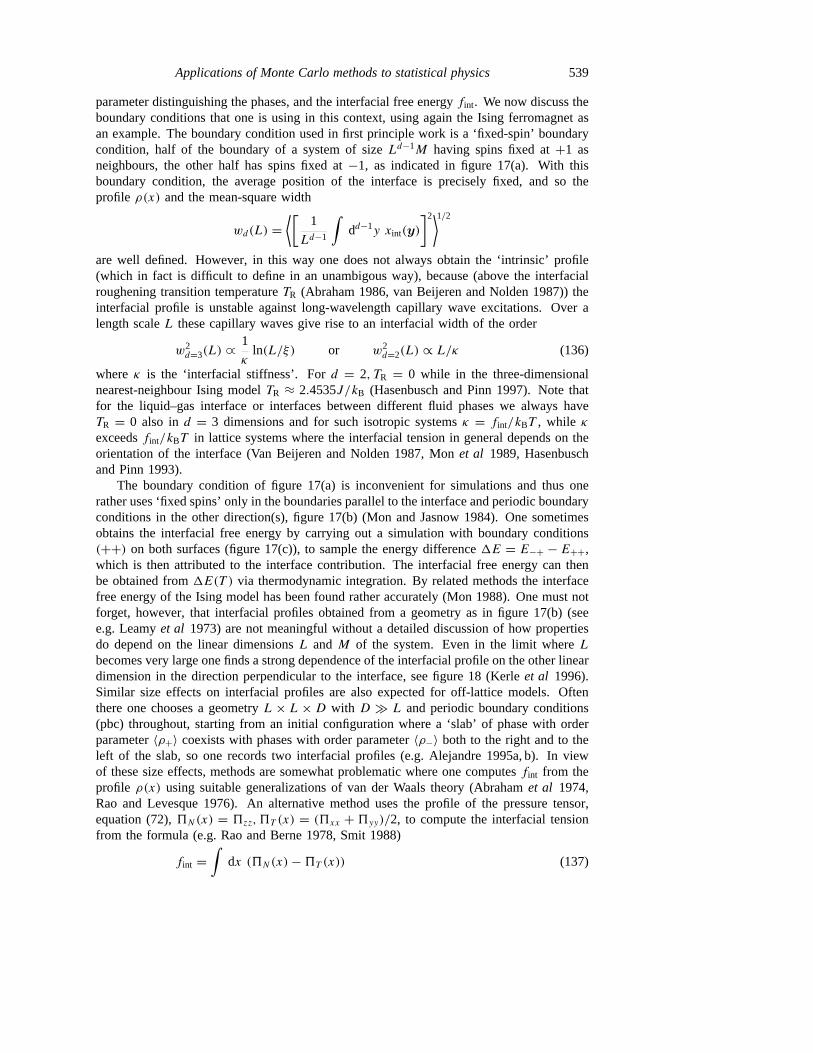
Applications of Monte Carlo methods to statistical physics 539
parameter distinguishing the phases, and the interfacial free energyfint. We now discuss theboundary conditions that one is using in this context, using again the Ising ferromagnet asan example. The boundary condition used in first principle work is a ‘fixed-spin’ boundarycondition, half of the boundary of a system of sizeLd−1M having spins fixed at+1 asneighbours, the other half has spins fixed at−1, as indicated in figure 17(a). With thisboundary condition, the average position of the interface is precisely fixed, and so theprofile ρ(x) and the mean-square width
wd(L) =⟨[
1
Ld−1
∫dd−1y xint(y)
]2⟩1/2are well defined. However, in this way one does not always obtain the ‘intrinsic’ profile(which in fact is difficult to define in an unambigous way), because (above the interfacialroughening transition temperatureTR (Abraham 1986, van Beijeren and Nolden 1987)) theinterfacial profile is unstable against long-wavelength capillary wave excitations. Over alength scaleL these capillary waves give rise to an interfacial width of the order
w2d=3(L) ∝
1
κln(L/ξ) or w2
d=2(L) ∝ L/κ (136)
whereκ is the ‘interfacial stiffness’. Ford = 2, TR = 0 while in the three-dimensionalnearest-neighbour Ising modelTR ≈ 2.4535J/kB (Hasenbusch and Pinn 1997). Note thatfor the liquid–gas interface or interfaces between different fluid phases we always haveTR = 0 also ind = 3 dimensions and for such isotropic systemsκ = fint/kBT , while κexceedsfint/kBT in lattice systems where the interfacial tension in general depends on theorientation of the interface (Van Beijeren and Nolden 1987, Monet al 1989, Hasenbuschand Pinn 1993).
The boundary condition of figure 17(a) is inconvenient for simulations and thus onerather uses ‘fixed spins’ only in the boundaries parallel to the interface and periodic boundaryconditions in the other direction(s), figure 17(b) (Mon and Jasnow 1984). One sometimesobtains the interfacial free energy by carrying out a simulation with boundary conditions(++) on both surfaces (figure 17(c)), to sample the energy difference1E = E−+ − E++,which is then attributed to the interface contribution. The interfacial free energy can thenbe obtained from1E(T ) via thermodynamic integration. By related methods the interfacefree energy of the Ising model has been found rather accurately (Mon 1988). One must notforget, however, that interfacial profiles obtained from a geometry as in figure 17(b) (seee.g. Leamyet al 1973) are not meaningful without a detailed discussion of how propertiesdo depend on the linear dimensionsL andM of the system. Even in the limit whereLbecomes very large one finds a strong dependence of the interfacial profile on the other lineardimension in the direction perpendicular to the interface, see figure 18 (Kerleet al 1996).Similar size effects on interfacial profiles are also expected for off-lattice models. Oftenthere one chooses a geometryL × L × D with D � L and periodic boundary conditions(pbc) throughout, starting from an initial configuration where a ‘slab’ of phase with orderparameter〈ρ+〉 coexists with phases with order parameter〈ρ−〉 both to the right and to theleft of the slab, so one records two interfacial profiles (e.g. Alejandre 1995a, b). In viewof these size effects, methods are somewhat problematic where one computesfint from theprofile ρ(x) using suitable generalizations of van der Waals theory (Abrahamet al 1974,Rao and Levesque 1976). An alternative method uses the profile of the pressure tensor,equation (72),5N(x) = 5zz,5T (x) = (5xx +5yy)/2, to compute the interfacial tensionfrom the formula (e.g. Rao and Berne 1978, Smit 1988)
fint =∫
dx (5N(x)−5T (x)) (137)

540 K Binder
Figure 18. The order parameter profile of the layer magnetizationmn against layer numbernof a nearest-neighbour Ising ferromagnet on the simple cubic lattice atT/Tcb = 0.9554, usinga L × L × D geometry with boundary fieldsH1/J = −0.55 at theL × L plane situated atn = 0, H1/J = +0.55 atn = D+ 1, andL = 128. Arrows show the values of the positive andnegative spontaneous magnetization,±mb. The table shows the values estimated for the widthw of the interface for the various thin film thicknessesD (all lengths being measured in unitsof the lattice spacing). From Kerleet al (1996).
the integration again being extended over the region of the interfacial profile (in thehomogeneous phases the pressure is isotropic, of course, and hence5N(x) = 5T (x)).Related formulae can also be used to obtain the surface free energy associated with walls(e.g. Pandeyet al 1997). We are not aware of any systematic investigation that size effectshave on equation (137), however.
For lattice systems such as Ising ferromagnets or antiferromagnets (Schmid and Binder1992a, b) it often is convenient to use, instead of the boundary condition of figure 17(b), anantiperiodic boundary condition (apbc). For example, for an Ising ferromagnet inD×L×Lgeometry this meansS(x ± D, y, z) = −S(x, y, z), with (x, y, z) being the coordinate ofthe lattice sitei. Then any perturbation by walls or boundary fields is strictly avoided, buta disadvantage is that this situation still has full translational invariance: the interface canbe anywhere in the system, and actually in the course of a Monte Carlo run will undergo adiffusive motion. If one wants to estimate the interfacial energy only, this delocalization ofthe interface does not matter; one simply has to obtain the free energy difference betweenthis system and a corresponding simulation with pbc,fint = D[Fapbc− Fpbc] (recalling thatF denotes a free energy per spin). For a study of interfacial profiles, one has to create asecond coordinate system, whose origin is fixed to the centre of the diffusing interface, andrecord profiles in this frame (Schmid and Binder 1992a, b).

Applications of Monte Carlo methods to statistical physics 541
If one is interested in the interfacial free energyfint only, a convenient method consistsin the sampling of how the minimum of the order parameter distributionPL(ρ) in between〈ρ+〉, 〈ρ−〉 decreases with increasing linear dimension (figure 17(d)). This technique (Binder1982) is particularly convenient, since it yieldsfint as a byproduct of a simulation of bulkproperties of the model system in aLd geometry. This method relies on the fact that, forL � ξ , the state of the system near the minimum is dominated by a configuration withtwo (on the average flat) domain walls running parallel to each other and to a lattice planethrough the system. Therefore, one expects
PL(ρ = ρmin) ∝ exp(−2Ld−1fint/kBT ) (138)
because the excess free energy cost of the configuration sketched in figure 17(d) is given bytwo interfaces of areaLd−1 each. The validity of equation (138) is checked by recordingPL(ρ) for a wide range ofL, noting that the probability should, forL � ξ , be nearlyconstant for a whole range ofρ aroundρmin, since changingρ then only changes the volumefraction of the two coexisting phases, but not their interfacial contributions. However, sincePL(ρ) from 〈ρ+〉, 〈ρ−〉 to ρmin varies over many orders of magnitude, one needs to apply‘multicanonical’ sampling in order to reach sufficient accuracy (Berg and Neuhaus 1992,Berget al 1993): after proper reweighting, an order parameter distribution which in between〈ρ−〉 and〈ρ+〉 is nearly flat is simulated. For the Ising magnet this so-called ‘multimagnetic’(Hansmannet al 1992) sampling has yielded very precise interfacial free energies (Berget al 1993) and the critical vanishing offint nearTc could be investigated. Even rathercomplex systems such as models for polymer mixtures have been successfully studied withthis technique (Muller et al 1995).
5. Miscellaneous topics
5.1. Applications to dynamic phenomena
In section 3.4 we have already seen that Monte Carlo (MC) sampling can be interpreted asa ‘time averaging’ along a stochastic trajectory through phase space, and this notion canbe made precise in terms of a Markovian master equation for the probabilityP(X, t) thatthe system is in stateX at time t (equation (47)). Of course, the dynamical propertiesof a system described by such a stochastic trajectory differs in general from dynamicproperties derived from a deterministic trajectory: remember that the molecular dynamics(MD) method amounts to solving Newton’s equation of motion numerically (Ciccotti andHoover 1986, Sprik 1996). In fact, for obtaining the dynamical properties of systems,such as simple Lennard-Jones fluids, MD is the only reasonable approach, and while theMC method is a perfectly valid approach for obtaining static properties of simple fluids inthermal equilibrium, the relaxation of density fluctuations seen in a MC run has nothing todo with the actual way that density fluctuations in fluids decay.
However, MC is a reasonable and useful method for describing dynamic properties ofsystems where the considered degrees of freedom are a slow subset of all degrees of free-dom. This slowness results from a weak coupling of these degrees of freedom to the fastones, which then act like a heat bath. A good example is the diffusion process in solidalloys (figure 1), where the phonons of the crystal act like a heat bath. Suppose we wouldsimulate such a mixed crystal at low temperatures by MD—most of the computer effortwould be spent for simulating the lattice vibrations (which typically have a time constantof 10−13 s), while the time constant on which jumps of A atoms or B atoms to vacant sitesoccur is orders of magnitude larger. It is easily possible then that in a MD run none (or only

542 K Binder
a few) such random jump events induced by the phonons are observed. While special MDtechniques exist to simulate the detailed properties of such rare events (Ciccotti and Ferrario1996), and such techniques are clearly useful for estimating the jump rates0A and0B forspecific materials, MD clearly is impractical to study the collective dynamic properties ontime scales large in comparison with the time scale of an isolated jump. If0A and0B canbe assumed as given parameters, the MC method can straightforwardly simulate directly therandom hopping processes (Kehret al 1989, Kehr and Binder 1984). The MC technique isunique also for simulating slow non-equilibrium processes, which happen on macroscopictime scales, such as the growth of ordered domains in adsorbed monolayers at surfaces(e.g. Sadiq and Binder 1984, Mouritsen 1990, Bray 1994), diffusion-limited growth of ag-gregates (Herrmann 1986, Meakin 1988), simulations of the growth of thin solid films viamolecular beam expitaxy and related techniques (e.g. Family and Vicsek 1991, Landau andPal 1996) etc. While these examples all refer to cases where one wishes to understand realsystems in terms of crudely simplified coarse-grained models, there exist also models suchas the Glauber kinetic Ising model (Glauber 1963, Kawasaki 1972) where a master equationdescription is postulated, not with the primary intention of describing any experimentallyaccessible systems but rather to elucidate general questions of statistical mechanics. In thiscontext we recall that Ising magnets do not have any dynamics of their own—spin flipsare thought to result as a consequence of a weak spin lattice coupling. These kinetic Isingmodels are of great interest to understand critical dynamics (Hohenberg and Halperin 1977)and MC methods have been used extensively for their study (e.g. Stollet al 1973, Landauet al 1989). Of course, one can also identify problems where both MC and MD approachescan be applied, for example, the slow Brownian motion of polymer chains in dense polymermelts (Binder 1995, Kremer and Grest 1990, 1995, Paulet al 1991). The MC method thenhas the advantage that unphysical ‘moves’ (crossing of chains, ‘slithering-snake’ motion,semigrand-canonical AB interchanges in mixtures, etc) are permissible to equilibrate thesystem: one may then set a clock to zero, at which point these unphysical moves are turnedoff, in order to study the further time evolution of the system applying an algorithm thatis physically reasonable (e.g. the random hopping algorithm of the bond fluctuation model,see Binder and Paul (1997) for a review). Of course, the MC dynamics does lack any hy-drodynamic mechanisms which, in principle, are present in MD work. In addition, the MCapproach can model only diffusive motions and relaxation, but does not account for oscilla-tory motions that are present in shorter time scales. Such limitations must be kept in mind inthe applications of MC methods to study the dynamics of polymers (Binder 1995) or otherslow processes: relaxation of the magnetization in spin glasses (Binder and Young 1986),relaxation of molecular orientation in quadrupolar glasses (Muser and Nielaba 1995), etc.
After this general overview we briefly treat one example in more detail, to illustrate thegreat potential of the approach, and the type of questions that one can address: interdiffusionin binary solid mixtures (figure 1). The considered degrees of freedom are occupationvariablescA
i , cBi of lattice sitesi which are unity if the sitei is taken by an A atom or a
B atom, respectively, and else zero. The phonons of the crystal then induce random hopswith jump rates0A and0B to vacant lattice sites.
We now recall the description of this problem in the framework of phenomenologicalnon-equilibrium thermodynamics: one postulates ‘constitutive equations’ for the currentdensitiesJA,JB of A, B atoms, namely linear relations between them and the drivingforces, the gradients of chemical potential differences between A(B) atoms and vacanciesV (µA − µV ,µB − µV ),
JA = −(3AA/kBT )∇(µA − µV )− (3AB/kBT )∇(µB − µV ) (139)

Applications of Monte Carlo methods to statistical physics 543
JB = −(3BA/kBT )∇(µA − µV )− (3BB/kBT )∇(µB − µV ). (140)
Here3AA ,3AB = 3BA,3BB are the ‘Onsager coefficients’. Equations (139) and (140) areat best approximately valid: nonlinearities and fluctuations are neglected. Taken togetherwith the continuity equations that express the conservation laws for the local concentrationscA(r, t), cB(r, t)
∂cA(r, t)/∂t +∇ · JA = 0 ∂cB(r, t)/∂t +∇ · JB = 0 (141)
it is a matter of simple algebra (Kehret al 1989) to obtain a complete description of theinterdiffusion process for a random alloy. For example, the interdiffusion constantDi ,which describes how a weak deviation of the concentration difference between A and Bfrom its average value spreads out, is given by
Di = 3AA3BB −32AB
3AA + 23AB +3BB
(1
cA+ 1
cB
)cV → 0. (142)
However, there are many questions about such a treatment: How are the Onsagercoefficients related to the atomistic rates0A, 0B (figure 1)? Is the ‘mean-field’ characterof equations (139) and (140) an accurate description? Etc. In particular, it is common toneglect the off-diagonal coefficient3AB (Brochardet al 1983, Krameret al 1984), sincenothing is known about it—but it is questionable whether3AB is really small in comparisonwith 3AA and3BB.
All these questions can be answered by ‘taylored’ computer experiments: by imposingchemical potential gradients either on the A atoms or on the B atoms one can createsteady-state currents in the system (particles leaving the box at one boundary re-enter at theopposite one, because of the periodic boundary conditons!). Thus the Onsager coefficientscan simply be measured from their definitions, equations (139) and (140). Figure 19 showsthat for0A/0B � 1 it is wrong to neglect0AB in comparison with0AA . However, usingthe so-determined Onsager coefficients in equation (142) provides an accurate descriptionof interdiffusion, as figure 20 shows.
Figure 20 also illustrates again that basic concepts of statistical physics can beimplemented very directly in simulations, such as linear response: one applies a wavevector-dependent chemical potential difference1µ(k)(k = 2π/λ) to the system, to prepare aninitial state of the model where a concentration wave with wavelengthλ is present. Inthe example shown, the amplitude is chosen such thatδcA(t = 0) = δcB(t = 0) = 0.02.At time t = 0, this perturbation1µ(k) is suddenly switched off, and then one simplywatches the decay of the concentration wave with time. Different wavelengths are used(figure 20) to check that one is actually in the long-wavelength limit. While the fullmean-field treatment (equation (142)) based on the actual Onsager coefficients works well,approximations (Brochardet al 1983, Krameret al 1984) where the Onsager coefficientsare somehow related to self-diffusion coefficients are not accurate in this case. Note thatself-diffusion coefficients are straightforwardly obtained from mean-square displacementsof tagged particles.
This is just one example out of many to show that MC simulations do have their placeto study dynamic phenomena. For more details, as well as a discussion of alternativeapproaches such as MD and Brownian dynamics (Ermak and McCammon 1978, vanGunsterenet al 1981, Doll and Dion 1976, Ciccotti and Ryckaert 1980, Giro et al 1985,Lemak and Balabaev 1995) where one numerically solves Langevin equations, we have torefer to the literature (Binder 1992b, Binder and Ciccotti 1996).
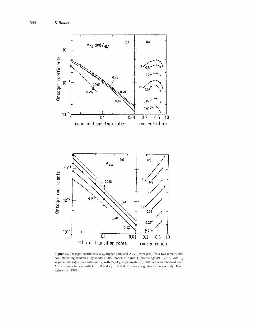
544 K Binder
Figure 19. Onsager coefficients3AB (upper part) and3AA (lower part) for a two-dimensionalnon-interacting random alloy model (ABV model, cf figure 1) plotted against0A/0B with cA
as parameter (a) or concentrationcA with 0A/0B as parameter (b). All data were obtained fromL × L square lattices withL = 80 andcV = 0.004. Curves are guides to the eye only. FromKehr et al (1989).

Applications of Monte Carlo methods to statistical physics 545
Figure 20. Amplitudes of concentration waves with wavelengthsλ as a function of timet (inunits of Monte Carlo steps (MCS) per particle), after a chemical potential variation with thesame wavelength has been shut off att = 0. Open circles represent A atoms, full dots B atoms,for a lattice ofL3 sites, withL = 80, cA = cB = 0.48, cV = 0.04, 0A/0B = 0.1. Threedifferent wavelengthsλ are shown (the arrow indicates the initial concentration amplitude forλ = 40). Note that one must chooseλν = L with ν integer, to comply with the periodicboundary conditions. The curves represent theoretical predictions, based on the use of actualOnsager coefficients (cf figure 19) in a mean-field theory based on equations (139)–(141) (forcV → 0 this theory predicts a single exponential decay proportional to exp[−Di(2π/λ)2t ] withDi given by equation (142), while for non-zerocV , cA(t) andcB(t) decay with superpositionsof two exponentials). From Kehret al (1989).
5.2. A brief introduction to path integral Monte Carlo (PIMC) methods
So far the discussions of this paper have been confined to the framework of classicalstatistical mechanics throughout. However, this is an approximation—the basic laws ofnature are quantum mechanical, and thus it is very important to be able to take quantumeffects into account in simulation techniques as well. Thus the development of MCtechniques to study ground-state as well as finite-temperature properties of interactingquantum many-body systems is an active area of research (for reviews see Ceperley andKalos, 1979, Schmidt and Kalos 1984, Kalos 1984, De Raedt and Lagendijk 1985, Berneand Thirumalai 1986, Suzuki 1986, 1992, Schmidt and Ceperley 1992, De Raedt and vonder Linden 1992, Hammondet al 1994, De Raedt 1996, Ceperley 1996, Kreer and Nielaba1996, Gubernatis and Kawashima 1996). These methods are of interest for a widespreadvariety of problems, including elementary particles (e.g. De Grand 1992), the structure ofatomic nuclei (e.g. Carlsson 1988), superfluidity of Helium (e.g. Schmidt and Ceperley1992), high-Tc superconductors (e.g. Fricket al 1990), hydrogen in metals (Gillan andChristodolous 1993), magnetism (e.g. Reger and Young 1988), surface physics (e.g. Marxet al 1993a b, Kreer and Nielaba 1996) isotope effects in lattice dynamics (Muser et al1995) etc. Here we cannot attempt to review all these applications, nor can we describeall the different techniques: variational Monte Carlo (VMC), Green’s function Monte Carlo(GFMC), projector Monte Carlo (PMC), path-integral Monte Carlo (PIMC), grand-canonical

546 K Binder
quantum Monte Carlo (GCMC), world-line quantum Monte Carlo (WLQMC), etc. We notethat some of these techniques are still under development, and there are sometimes seriousproblems hampering large-scale applications (such as the famous ‘minus sign problem’hampering the applications to multifermion systems, see e.g. De Raedt and von der Linden(1992)). Here we shall not address any methods for ground-state properties (like VMC,GFMC), but are concerned with the PIMC method that only addresses properties at non-zero temperatures.
Unlike equation (3) we now consider an average〈A〉 where the HamiltonianH istreated as a quantum-mechanical operator, and we do not assume that the eigenvalues andeigenstates ofH are known explicitly,
〈A〉 = (1/Z)Tr exp(−H/kBT )A Z = Tr exp(−H/kBT ). (143)
Here A is the operator associated with the classical observableA(X) in equation (3). Forsimplicity, we consider first a single particle in one dimension exposed to a potentialV (x),for which H = −(h2/2m) d2/dx2+ V (x). In position representation (|x〉 is an eigenvectorof the position operator) the partition function becomes
Z =∫
dx〈x| exp(−H/kBT )|x〉. (144)
Equation (144) is not straightforward to evaluate since the operators of kinetic energy{−(h2/2m) d2/dx2} and potential energy{V (x)} do not commute. Writing exp(−H/kBT )
formally as [exp(−H/kBT P )]P , whereP is a positive integer, we can insert a completeset of states between the factors:
Z =∫
dx1 . . .
∫dxp〈x1| exp(−H/kBT P )|x2〉〈x2| . . . |xp〉〈xp| exp(−H/kBT P )|x1〉. (145)
For largeP , it is a good approximation to ignore the fact that kinetic and potential energydo not commute. Hence one gets
〈x| exp(−H/kBT P )|x ′〉 ≈(kBTmP
2πh2
)1/2
exp
{−kBTmP
2πh2 (x − x ′)2}
× exp
{− 1
2kBT P[V (x)+ V (x ′)]
}(146)
and thus
Z =(kBTmP
2πh2
)P/2 ∫dx1 . . .
∫dxp
× exp
{− 1
kBT
[1
2
P∑S=1
κ(xS − xS+1)2+ P−1
P∑S=1
V (xS)
]}(147)
whereκ = kBTmP/h2. In the limit P → ∞, equation (147) becomes exact. Apart from
the prefactor, equation (147) is precisely the configurational partition function of a classicalsystem, namely a ring polymer consisting ofP beads coupled by harmonic springs withspring constantκ, each bead being under the action of a potentialV (x)/P .
This approach is straightforwardly generalized to a system ofN interacting quantumparticles—one ends up with a system ofN classical cyclic ‘polymer chains’. However, animportant distinction from physical melts of ring polymers is that in the present case beadsof different chains interact with each other only if they are in the same ‘time slice’ (i.e.have the same ‘Trotter index’s).

Applications of Monte Carlo methods to statistical physics 547
As a result of this isomorphism, classical MC methods can be readily applied to samplesuch quantum-mechanical problems. At high temperatures,κ becomes very large, and thenthe system always behaves classically, since then the cyclic chains contract essentially topoint particles again. At low temperatures, however, they are spread out over distancescomparable to the thermal de Broglie wavelength, and in this way zero-point motions arealso accounted for. However, PIMC becomes increasingly difficult at low temperatures,sinceP has to be the larger the lowerT : if σ is a characteristic distance over which thepotentialV (x) changes, one must have ¯h2/mσ 2 � kBT P in order that two neighboursalong the ‘polymer chain’ are at a distance much smaller thanσ . The appropriate valueof this ‘Trotter dimension’P is determined empirically in most cases (typically one carriesout runs for several choices ofP and checks where thermal properties no longer change).
The step leading to equation (146) can be viewed as a special case of the Suzuki–Trotterformula (e.g. Suzuki 1986)
exp(A+ B) = limP→∞
[exp(A/P ) exp(B/P )]P . (148)
Equation (148) is used for mappingd-dimensional quantum problems on lattices toequivalent classical problems in(d + 1) dimensions: for example, the Ising chain in atransverse magnetic field gets mapped onto a special two-dimensional Ising lattice, with alinear dimensionP in the additional ‘Trotter direction’ (which corresponds to the imaginarytime direction of the path integral).
For rigid molecules the operator of angular momentum appears inH in equation (144)and this requires another extension of the formalism. The fact that a rotation with an angleof 2π leaves the physical situation invariant creates subtle problems. For two-dimensionalrotators (confined to rotate in a plane) the rotation angleϕ plays a similar role as thecoordinatex in equation (147), but in addition one has a summation over ‘winding numbers’expressing the fact of how many multiples of 2π the angle passes along the ring polymer(Marx and Nielaba 1992, Marxet al 1993b). Then in addition to ‘local’ Monte Carlo movesϕs → ϕ′s , which conserve the winding number, ‘global’ moves are also needed to changethe winding number. For rotators with two angular degrees of freedom one runs again into‘minus sign’ problems (Marx 1994, Muser 1996)!
As an example for the type of questions that one can address, figure 21 shows the orderparameter and energy of N2 adsorbed on graphite (Marxet al 1993a). It is seen that quantumfluctuations depress the temperature of the order–disorder transition (which is rounded dueto finite-size effects, of course) by about 10%, and the order parameter saturates at 90% ofits classical value due to zero-point vibrations. While the latter behaviour is accounted forby quasi-harmonic theory, and the former effect could be accounted for by the Feynman–Hibbs approximation, there is in fact no approximate treatment accurate at temperaturesin the ordered phase just below the transition. Note that such simulations are still ratherdifficult, since Trotter dimensions up toP = 500 needed to be used.
5.3. Some recent algorithmic developments
The availability of vector processors and of massively parallel supercomputers has made itnecessary to develop Monte Carlo codes that take advantage of this specialized hardwareand are optimized in order to perform on such machines as fast as possible (Landau 1992,Heermann and Burkitt 1992, Heermann 1996). We shall not give any details on theseproblems here. We only mention that one always heavily exploits the freedom that one hasin MC calculations (of static averages) in defining the precise order in which one carries outupdating operations in the configurations of the system. For example, for simulating Ising-

548 K Binder
Figure 21. Herringbone structure order parameter for N2 adsorbed on graphite plotted againsttemperature. The centre of gravity of the 900 N2 molecules is fixed in the plane where thegraphite potential (as parametrized by Steele (1978)) has its minimum on the regular sitesof a triangular lattice, allowing only for one rotational degree of freedom(ϕ) per molecule.Apart from the corrugation potential, nitrogen atoms interact with Lennard-Jones forces andquadrupole–quadrupole interactions. Full curve, quantum simulation; dotted curve, classicalsimulation; dashed curve, quasiharmonic theory; triangles, Feynman–Hibbs expansion aroundclassical path. The inset shows corresponding data for the energy. From Marxet al (1993a).
type lattice models on vector processors it is preferable not to go through the lattice sites inthe standard typewriter-type fashion, but rather to decompose the lattice in sublattices suchthat the degrees of freedom on one sublattice do not interact with each other (for a nearest-neighbour Ising square lattice, this is already achieved by the well known ‘checkerboarddecomposition’ into a ‘white’ and a ‘black’ sublattice, introduced by Oed (1982) for thefloating point system AP-190L and used for a study of the Ising model interfacial tension(Binder 1982)). In combination with multispin coding (multiple spins of one system arepacked in a single word, as first suggested by Zornet al (1981)) or multilattice simulations(spins from 64 different lattices are packed into 64 bit words, see Bhanotet al (1986))very efficient algorithms result, as described in detail by Landau (1992). The principle ofthis checkerboard algorithm, that degrees of freedom which lack a direct interaction can beupdated independently, is the basis of many related applications (e.g. spin-exchange kineticIsing models (Zhang 1989, Amaret al 1988), random Ising models (Heuer 1990) or Pottsmodels (Eichhorn and Binder 1995, 1996), lattice models for alloys (Dunweg and Binder1987), and polymer melts (Wittmann and Kremer 1990, 1992) etc).
At the time of writing, vector processors are losing ground in comparison to parallelsupercomputers. The concepts for efficient use of parallel processors are rather similar tothose used in ‘vectorization’ of programs—one has to identify tasks that can be carriedout independently and concurrently. A straightforward idea is ‘domain decomposition’, i.e.the system is geometrically decomposed into subsystems. For systems with short-rangeinteractions, interactions between degrees of freedom belonging to different subsystems

Applications of Monte Carlo methods to statistical physics 549
occur only in a rather narrow boundary region of each subsystem. If these subsystems arethemselves sufficiently large, the overhead for communication between processors can bemade sufficiently small in practice (Heermann and Burkitt 1992, Heermann 1996). Usefulapplications result when the physics of the problem requires large total system sizes, forexample, interfaces in polymer mixtures were simulated on lattices containing about 16million sites (Muller et al 1995), and simple Ising square lattices up to size of 106 × 106
could be studied (Linkeet al 1995, 1996). Of course, other strategies of parallelizationmay be preferable for different applications: performing the MC approach with long-rangeinteractions, one may simply split the ensemble ofN particles intop portions ofN/pparticles; each processor then calculates the energy change of one of these portions in anMC update. Even simpler is a method that is sometimes called ‘poor man’s parallelization’(Heermann 1996): the system is simply replicatedp times; each processor carries outthe same program but with different random numbers (and perhaps also with a differentstarting configuration), and so the only communication among processors that is needed isthe averaging of the results from individual processors in order to obtain the final results.This approach is very natural for systems containing randomly quenched disorder (Eichhornand Binder 1995): one has to carry out the average [. . .]av over the quenched disorder byaveraging over a large number of equivalent replicas of the system, each containing adifferent realization of the variables characterizing the quenched disorder (random bonds,random fields, randomly diluted sites, etc); thus this disorder average is done in parallel,each processor working on its own replica of the system.
Another very important line of research on Monte Carlo algorithms considers theconstruction of clever moves for the MC updates in order to sample the phase space mostefficiently, i.e. to decorrelate successive configurations as fast as possible. For example, forthe Ising model at the critical temperatureTc the standard single spin-flip algorithm suffersfrom the problem of ‘critical slowing down’ (Hohenberg and Halperin 1977), which meansin a finite-size scaling context that the relaxation timeτ scales with the linear dimensionlike τ ∝ Lz, z being the ‘dynamic exponent’ of the model (z ≈ 2). Many ideas havebeen followed to ease this problem: Fourier acceleration (e.g. Batrouniet al 1985, Dagottoand Kogut 1987), multigrid MC (Goodman and Sokal 1986, 1989, Kandelet al 1989,Hasenbuschet al 1991, Janke and Sauer 1994, 1995), over-relaxation (Creutz 1987) etc.The most successful approach seems to be the cluster algorithms (Swendsen and Wang 1987,Wolff 1988a, b, Wolff 1989a, b, c, Edwards and Sokal 1988, 1989, Ben-Avet al 1990, Wanget al 1990, Kandel and Domany 1991, Swendsenet al 1992, Machtaet al 1995, Liverpooland Glotzer 1996, Luijten and Blote 1996) based on the mapping (Fortuin and Kasteleyn1972) between Potts models and percolation (see section 4.2). For ferromagnetic Ising, Potts,and vectorspin models these algorithms reduce the dynamic exponentz to a very small value(in favourable casesz = 0, e.g. for the single cluster algorithm (Wolff 1989a) ind > 4dimensions, see Tamayoet al (1990)). While extensions exist to antiferromagnetic Pottsmodels (Wanget al 1990), interfaces in solid-on-solid models and Ising models (Hasenbuschand Meyer 1991, Hasenbusch and Pinn 1997), and quantum MC problems (Gubernatis andKawashima 1996), so far this approach could not be generalized to off-lattice problems, andalso many lattice problems involving frustration (spinglasses, lattice gauge problems, etc)still await the formulation of a useful cluster algorithm.
A very promising approach also is the combination of cluster algorithms withother advanced methods, for example, with multigrid MC (Kandelet al 1989) or withmulticanonical sampling (the so-called ‘multibondic algorithm’ (Janke and Kappler 1995)).
A recently developed method that works both for lattice and off-lattice problems andhas interesting parallels to cluster algorithms (Frenkel 1993) is the so-called ‘configurational

550 K Binder
bias Monte Carlo’ (CBMC) method (Siepmann 1990, Siepmann and Frenkel 1992, de Pabloet al 1992). This method was originally invented for macromolecules but is presumablyuseful for many other problems (see Frenkel (1993) and Frenkel and Smit (1996) for moredetails).
While in the techniques mentioned above the dynamics of the Monte Carlo ‘clustermoves’ clearly is unphysical, and there is no connection in an Ising simulation using acluster algorithm with the dynamics of a single spin-flip algorithm, techniques have alsobeen developed (e.g. use of absorbing Markov chains (Novotny 1995) or rescaling techniquesinspired by the renormalization group ideas, see Barkema and Marko (1993)). For studyingnucleation kinetics in Ising models at low temperatures or the dynamics of coarsening in thesimulation of quenching experiments one can observe dynamic processes over 25 decadesin time—a task that would be impossible for straightforward dynamic MC techniques.
Finally we mention the reweighting techniques (see Dunweg (1996) and Frenkel andSmit (1996) for recent reviews). The ‘single histogram method’ starts from the observationthat the energy distribution at temperatureT can be obtained from the distributionP(E, T0)
at a neighbouring temperatureT0 by
P(E, T ) = P(E, T0) exp[−(1/T − 1/T0)E/kB]
/∑E
(E, T0) exp[−(1/T − 1/T0)E/kB].
(149)
This idea is not at all new (Salsburget al 1959) but has only recently been very widelyused—first of all one can now generate ‘histograms’P(E, T0) with the necessary statisticalaccuracy, which was not possible in the early days of Monte Carlo, and second it wasrecognized by Ferrenberg and Swendsen (1988) that at a critical point the width of thedistribution due to critical fluctuations is sufficiently broadened to allow a reweighting overthe temperature interval|T − Tc| of order L−1/ν , i.e. the region of interest for a finite-size scaling analysis, irrespective of the linear dimensionL. In particular, the combineduse of several histograms at suitably chosen neighbouring temperatures (or other controlparameters), the so-called ‘multiple histogram extrapolation’ (Ferrenberg and Swendsen1989, Swendsenet al 1992) has become a standard tool in the study of critical phenomena.We emphasize that one can perform a reweighting in several parameters simultaneously (e.g.temperature and chemical potential, in a study of criticality in fluids, see Wilding (1996)).Reweighting densities is also possible and is called ‘density scaling’ (Valleau 1993).
Particularly useful are also reweighting schemes built into the simulation procedure(‘umbrella sampling’ (Valleau and Torrie 1977), ‘multicanonical MC’ techniques (Berg andNeuhaus 1992), ‘entropic sampling’ (Lee 1993), the ‘broad histogram method’ (de Oliveiraet al 1996) etc). Basically, one is sampling the states not with the Boltzmann probability(∝ exp(−H/kBT )) but with a modified probability (∝ exp(−Heff/kBT )). This will producean energy distribution
P(E) = exp[S(E)−Heff/kBT ]
/∑E
exp[S(E)−Heff/kBT ]. (150)
The optimal choice would be ifP(E) were flat, i.e. ifHeff/kBT is just the entropy (apartfrom an additive constant). Thus one could proceed in an iterative way, choosing firstH(0)eff = E/kBT0 for some reasonableT0, estimatingP(E) via a histogram, and then usingH(1)eff = H(0)eff + ln(P (E)R), R being the total number of energy entries, etc. Of course, onemust be very careful that the runs are long enough so thatP(E) is reliably estimated. Inthe end, thermal averages of observablesA are then obtained as
〈A〉T = 〈A exp[(Heff −H)kBT ]〉/〈exp[(Heff −H)/kBT ]〉. (151)

Applications of Monte Carlo methods to statistical physics 551
Such techniques are particularly useful to study first-order transitions, and to obtaininterfacial tensions between coexisting phases, as discussed in section 4.4.
A related approach (‘simulated tempering’ (Marinari and Parisi 1992), ‘expandedensemble’ (Lyubartsevet al 1992)) considers the temperature just as an additional degree offreedom, specifying properly transition rules for jumping from one temperature to another.
Clearly, all we could give here was a sketchy guide to the original literature in a rapidlydeveloping and very promising field! But it is clear that algorithmic developments are asimportant as improvements in the computer performance for the growing impact of MonteCarlo simulation in statistical physics.
6. A few concluding remarks
In this review, we have attempted to provide an introductory and tutorial overview of MonteCarlo simulation, primarily addressed to the non-specialist. Thus we have given the basicaspects of the technique in some detail, and we have also described in some depth thefinite-size effects, which, on the one hand, seriously hamper all simulation work, but, onthe other, can also be used as a tool for extracting quantitatively reliable predictions on bulkand interfacial properties, via the appropriate finite-size scaling considerations.
In presenting these points, we have chosen to illustrate them with material exclusivelytaken from the research group of the author. It must be stressed that this choice of exampleswas purely a matter of convenience only, and it should be clear from the extensive listof references that many groups have contributed very significantly to the development oftechniques that were described here. Thus the bias in the choice of examples should not beat all mistaken as a statement on the validity and/or importance of other results.
In this review, we have also chosen to emphasize classical MC work on equilibriumproperties of lattice models, and have dealt only very briefly with topics such as thestatistical mechanics of off-lattice models, non-equilibrium phenomena such as simulationsof irreversible growth, and quantum problems in statistical thermodynamics. Thus we haveonly tried to give the reader a flavour of what can be done and what new problems arisewhen one applies MC methods in these fields. The same disclaimer holds with respectto the many clever algorithms that have been devised to carry out simulations in a moreefficient way—we only intended to ‘wet the readers appetite’ to the rich literature on allthese interesting problems and approaches.
Nevertheless, we hope that this review can give a clear hint to the usefulness of thesecomputer simulation methods, and the challenge they pose in their proper application andtheir use as a powerful tool of research. Also, with respect to the technical aspects of this‘tool’, it is clear that this review could only describe ‘work in progress’, so there is stillmuch room for good ideas for the further refinement of the technique and for developingapplications to new problems, and thus one can understand the fascination that the computersimulation approach has, leading to a truly explosive growth of the literature in this area.
Acknowledgments
The author’s knowledge of the subject has slowly grown in a longstanding and verystimulating interaction with numerous coworkers and colleagues. At this point I can thankonly a few of them, to whom I am particularly indebted, since I have used material fromjoint research for this review, in particular D P Landau, D W Heermann and K Kremer,and also H-P Deutsch, B Dunweg, E Eisenriegler, R Evans, A M Ferrenberg, J D Gunton,

552 K Binder
S Kammerer, K Kaski, K W Kehr, D Marx, M D’Onorio de Meo, H Muller-Krumbhaar,P Nielaba, O Opitz, J D Reger, S Reulein, M Scheucher, D Stauffer, and K Vollmayr.
References
Abraham D B 1986Phase Transitions and Critical Phenomenavol 10, ed C Domb and J L Lebowitz (London:Academic)
Abraham F F 1974Homogeneous Nucleation Theory(New York: Academic)Abraham F F, Schreiber D E and Barker J 1974J. Chem. Phys.60 1976Albano E V, Binder K, Heermann D W and Paul W 1989aZ. Phys.B 77 445——1989bJ. Chem. Phys.91 3700Alder B J and Wainwright T E 1962Phys. Rev.127 359Alejandre J, Tildesley D F and Chapela G A 1995aMol. Phys.85 651——1995bJ. Chem. Phys.102 4574Alexandrowicz Z 1975J. Stat. Phys.13 231——1976J. Stat. Phys.14 1Allen M P 1996Monte Carlo and Molecular Dynamics of Condensed Matter Systemsed K Binder and G Ciccotti
(Bologna: Italian Physical Society) p 255Allen M P and Tildesley D J 1987Computer Simulation of Liquids(Oxford: Clarendon)——(eds) 1993Computer Simulation in Chemical Physics(Dordrecht: Kluwer)Amar J G, Sullivan F E and Mountain R D 1988Phys. Rev.B 37 196Baker G A Jr andKawashima N 1995Phys. Rev. Lett.75 994——1996J. Phys. A: Math. Gen.29 7183Barber M N 1983 Phase Transitions and Critical Phenomenavol 8, ed C Domb and J L Lebowitz (New York:
Academic) p 145Barkema G T and Marko J F 1993Phys. Rev. Lett.71 2030Batoulis I and Kremer K 1988J. Phys. A: Math. Gen.21 127Batrouni G G, Katz G R, Kronfeld A S, Lepage G P, Svetitsky B and Wilson K G 1985Phys. Rev.D 32 2376Baumgartner A 1985J. Polym. Sci. C Symp.73 181Ben-Av R, Kandel D, Katznelson E, Lauwers P G and Solomon S 1990J. Stat. Phys.58 125Berg B A 1992Dynamics of First Order Phase Transitionsed H J Herrmann, W Janke and F Karsch (Singapore:
World Scientific)Berg B A, Hansmann U and Neuhaus T 1993Z. Phys.B 90 229Berg B A and Neuhaus T 1992Phys. Rev. Lett.68 9Berne B J and Thirumalai D 1986Ann. Rev. Phys. Chem.37 401Bhanot G, Creutz M and Neuberger H 1984Nucl. Phys.B 235 417Bhanot G, Duke D and Salvador R 1986J. Stat. Phys.44 985Billoire A, Lacaze R and Morel A 1992Nucl. Phys.B 370 773Billoire A, Neuhaus T and Berg B A 1993Nucl. Phys.B 396 779Binder K 1972Physica62 508——1974Thin Solid Films20 367——1976Ann. Phys.98 390——1981aZ. Phys.B 43 119——1981bZ. Phys.B 45 61——1982Phys. Rev.A 25 1699——1983J. Chem. Phys.79 6387——1985Z. Phys.B 61 13——1986Advances in Solid State Physicsvol 26, ed P Grosse (Braunschweig: Vieweg) p 133——1987aFerroelectrics73 43——1987bRep. Progr. Phys.50 783——1992aComputational Methods in Field Theoryed H Gausterer and C B Lang (Berlin: Springer) p 59——(ed) 1992bThe Monte Carlo Method in Condensed Matter Physics(Berlin: Springer)——(ed) 1995 Monte Carlo and Molecular Dynamics Simulations in Polymer Science(New York: Oxford
University Press)Binder K, Bowker M, Inglesfield J E and Rous P J 1995Cohesion and Structure of Surfaces(Amsterdam: Elsevier)Binder K and Ciccotti G (ed) 1996Monte Carlo and Molecular Dynamics of Condensed Matter Systems(Bologna:
Italian Physical Society)

Applications of Monte Carlo methods to statistical physics 553
Binder K and Deutsch H P 1992Europhys. Lett.18 667Binder K, Evans R, Landau D P and Ferrenberg A M 1996 Phys. Rev.E 53 5023Binder K and Heermann D W 1988Monte Carlo Simulation in Statistical Physics. An Introduction(Berlin:
Springer)Binder K and Hohenberg P C 1974Phys. Rev.B 9 2194Binder K and Kalos M H 1979Monte Carlo Methods in Statistical Physicsed K Binder (Berlin: Springer) ch 6——1980J. Stat. Phys.22 363Binder K and Landau D P 1980Phys. Rev.B 21 1941——1984Phys. Rev.B 30 1477——1989Molecule–Surface Interactioned K P Lawley (New York: Wiley) p 91——1992J. Chem. Phys.96 1444Binder K, Landau D P and Wansleben S 1989Phys. Rev.B 40 6971Binder K, Nauenberg M, Privman V and Young A P 1985Phys. Rev.B 31 1498Binder K and Paul W 1997J. Polym. Sci., Part B: Polymer Phys.35 1Binder K, Rauch H and Wildpaner V 1970J. Phys. Chem. Solids31 391Binder K and Reger J D 1992Adv. Phys.41 547Binder K and Sillescu H 1989Encyclopedia of Polymer Science and Engineering (suppl. vol)ed H Mark (New
York: Wiley) p 297Binder K and Stauffer D 1972J. Stat. Phys.6 49——1976Adv. Phys.25 343Binder K and Wang J S 1989J. Stat. Phys.55 87Binder K and Young A P 1986Rev. Mod. Phys.58 801Blote H W J andNightingale M P 1982PhysicaA 112 405Borgs C and Kappler S 1992Phys. Lett.171A 37Borgs C and Kotecky K 1990J. Stat. Phys.61 79Borgs C, Kotecky R and Miracle-Sole S 1991J. Stat. Phys.62 529Bortz A B, Kalos M H and Lebowitz J L 1975J. Comput. Phys.17 10Bray A J 1994Adv. Phys.43 357Brezin E 1982J. Physique43 15Brezin E and Zinn-Justin J 1985Nucl. Phys.B 257 [FS14] 867Brochard F, Jouffray J and Levinson P 1983Macromolecules16 2638Brown R G and Ciftan M 1996Phys. Rev. Lett.76 1352Bruce A D 1997PreprintCardy J L and Nightingale M P 1983Phys. Rev.B 27 4256Carlsson J 1988Phys. Rev.C 38 1879Carmesin I and Kremer K 1988Macromolecules21 2819Ceperley D M 1996Monte Carlo and Molecular Dynamics of Condensed Matter Systemsed K Binder and G Ciccotti
(Bologna: Italian Physical Society) p 443Ceperley D M and Kalos M H 1979Monte Carlo Methods in Statistical Physicsed K Binder (Berlin: Springer)
p 145Challa M S S andHetherington J H 1988Phys. Rev.A 38 6324Challa M S S,Landau D P and Binder K 1986Phys. Rev.B 34 1841Ciccotti G and Ferrario M 1996Monte Carlo and Molecular Dynamics of Condensed Matter Systemsed K Binder
and G Ciccotti (Bologna: Italian Physical Society) p 107Ciccotti G and Hoover W G (eds) 1986Molecular Dynamics of Condensed Matter Systems(Amsterdam: North-
Holland)Ciccotti G and Ryckaert J-P 1980Mol. Phys.40 141Compagner A 1991Amer. J. Phys.59 700——1995Phys. Rev.E 52 5634Compagner A and Hoogland A 1987J. Comput. Phys.71 391Coniglio A and Klein W 1980J. Phys. A: Math. Gen.13 2775Creutz M 1983Phys. Rev. Lett.50 1411——1987Phys. Rev.D 36 515Dagotto E and Kogut J 1987Phys. Rev. Lett.58 299de Gennes P G 1979Scaling Concepts in Polymer Physics(Ithaca, NY: Cornell University Press)De Grand T 1992Computational Methods in Field Theoryed H Gausterer and C B Lang (Berlin: Springer) p 159de Oliveira P M C,Penna T J P andHerrmann H J 1996Brazilian J. Phys.26 677de Pablo J J, Laso M and Suter U W 1992J. Chem. Phys.96 2394

554 K Binder
De Raedt H 1996Monte Carlo and Molecular Dynamics of Condensed Matter Systemsed K Binder and G Ciccotti(Bologna: Societa Italiana di Fisica) p 401
De Raedt H and Lagendijk 1985Phys. Rep.127 233De Raedt H and von der Linden 1992The Monte Carlo Method in Condensed Matter Physicsed K Binder (Berlin:
Springer) p 249Desai R C, Heermann D W and Binder K 1988J. Stat. Phys.53 795Deutsch H-P 1993J. Chem. Phys.99 4825Deutsch H-P and Binder K 1992Macromolecules25 6214——1993aJ. Physique II3 1049——1993bMacromol. Symp.65 59Dietrich S 1988Phase Transitions and Critical Phenomenavol XII, ed C Domb and J L Lebowitz (London:
Academic) p 1Di Tolla F D, Tosatti E and Ercolesi F 1996Monte Carlo and Molecular Dynamics of Condensed Matter Systems
ed K Binder and G Ciccotti (Bologna: Societa Italiana di Fısica) p 345Doll J D and Dion D R 1976J. Chem. Phys.65 3762Domb C and Green M S (eds) 1976Phase Transitions and Critical Phenomenavol 6 (London: Academic)D’Onorio de Meo M, Heermann D W and Binder K 1990J. Stat. Phys.60 585D’Onorio de Meo M, Reger J D and Binder K 1995PhysicaA 220 628Dunweg B 1996Monte Carlo and Molecular Dynamics of Condensed Matter Systemsed K Binder and G Ciccotti
(Bologna: Italian Physical Society) p 215Dunweg B and Binder K 1987Phys. Rev.B 36 6935Edwards R G and Sokal A D 1988 Phys. Rev.D 38 2009——1989Phys. Rev.D 40 1374Eichhorn K and Binder K 1995Europhys. Lett.30 331——1996J. Phys.: Condens. Matter8 5209Eisenriegler E, Kremer K and Binder K 1982J. Chem. Phys.77 6296Ermak D L and Mc Cammon J A 1978J. Chem. Phys.69 1352Escobedo F A and de Pablo J J 1995J. Chem. Phys.103 2703Family F and Vicsek T 1991Dynamics of Fractal Surfaces(Singapore: World Scientific)Feder J 1988Fractals (New York: Plenum)Ferrenberg A M and Landau D P 1991Phys. Rev.B 44 5081Ferrenberg A M, Landau D P and Wong Y J 1992Phys. Rev. Lett.69 3382Ferrenberg A M and Swendsen R H 1988Phys. Rev. Lett.61 2635——1989Phys. Rev. Lett.63 1195Fisher M E 1967Physics3 267——1971Critical Phenomenaed M S Green (New York: Academic) p 1——1974Rev. Mod. Phys.46 587Fisher M E and Berker N A 1982 Phys. Rev.B 26 2507Fisher M E and Nakanishi H 1981J. Chem. Phys.75 5857Fisher M E and Privman V 1985Phys. Rev.B 32 447Fortuin C M and Kasteleyn P W 1972Physica57 536Freirie F, O’Connor D and Stephens C R 1994J. Stat. Phys.74 219Frenkel D 1993Computer Simulation in Chemical Physicsed M P Allen and D J Tildesley (Dordrecht: Kluwer)
p 93Frenkel D and Smit B 1996Understanding Molecular Simulation: From Algorithms to Applications(New York:
Academic)Frick M, Pattnaik P C, Morgenstern I, Newns D M and von der Linden 1990Phys. Rev.B 42 2665Furukawa H and Binder K 1982Phys. Rev.A 26 556Gerling R W and Huller A 1993Z. Phys.B 90 207Gillan M J and Christodolous F 1993Int. J. Mod. Phys.C 4 287Giro A, Guardia E and Padro J A 1985Mol. Phys.55 1063Glauber R J 1963J. Math. Phys.4 293Goodman J and Sokal A D 1986 Phys. Rev. Lett.56 1015——1989Phys. Rev.D 40 2035Gross D H E, Ecker A and Zhang X Z 1996Ann. Phys.5 446Gubernatis J E and Kawashima N 1996Monte Carlo and Molecular Dynamics of Condensed Matter Systemsed
K Binder and G Ciccotti (Bologna: Italian Physical Society) p 519Gunton J D, San Miguel M and Sahni P S 1983Phase Transitions and Critical Phenomenavol 8, ed C Domb and

Applications of Monte Carlo methods to statistical physics 555
J L Lebowitz (New York: Academic) p 267Guttmann A J 1989Phase Transitions and Critical Phenomenavol 13, ed C Domb and J L Lebowitz (London:
Academic)Hammersley J M and Handscomb D C 1964Monte Carlo Methods(London: Chapman and Hall)Hammond B L, Lester W A Jr and Reynolds P J 1994Monte Carlo Methods in ab initio Quantum Chemistry
(Singapore: World Scientific)Hammrich O 1993Z. Phys.B 92 501Hansmann U, Berg B A and Neuhaus T 1992Int. J. Mod. Phys.C 3 1155Harris R 1985Phys. Lett.111A 299Hasenbusch M and Meyer S 1991Phys. Rev. Lett.66 530Hasenbusch M, Meyer S and Mack G 1991Nucl. Phys. (Proc. Suppl)B 20 110Hasenbusch M and Pinn K 1993PhysicaA 192 342——1997J. Phys. A: Math. Gen.30 63Heermann D W 1996Monte Carlo and Molecular Dynamics of Condensed Matter Systemsed K Binder and G
Ciccotti (Bologna: Italian Physical Society) p 887Heermann D W and Burkitt A N 1990 PhysicaA 162 210——1992The Monte Carlo Method in Condensed Matter Physics(Berlin: Springer) p 53Heermann D W and Stauffer D 1980Z. Phys.B 40 133Herrmann H J 1986Phys. Rep.136 143Herrmann H J, Janke W and Karsch F (eds) 1992Dynamics of First Order Phase Transitions(Singapore: World
Scientific)Heuer H-O 1990Comput. Phys. Commun.59 387Hill T L 1956 Statistical Mechanics(New York: McGraw-Hill)——1963Thermodynamics of Small Systems(New York: Benjamin)Hohenberg P C and Halperin B I 1977Rev. Mod. Phys.49 435Holm C and Janke W 1997Phys. Rev. Lett.Hu C K 1984Phys. Rev.B 29 5103Hu C K and Mak S K 1989Phys. Rev.B 40 5007Huller A 1992Z. Phys.B 88 79——1994Z. Phys.B 95 63Imry Y 1980 Phys. Rev.B 21 2042——1984J. Stat. Phys.34 849Ito N and Suzuki M 1991Phys. Rev.B 43 3483James F 1990Comput. Phys. Commun.60 329Janke W 1994Computer Simulation Studies in Condensed Matter Physics VIIed D P Landau, K K Mon and H-B
Schuttler (Berlin: Springer) p 29Janke W and Kappler S 1995Phys. Rev. Lett.74 212Janke W and Sauer T 1994Nucl. Phys. (Proc. Suppl.)B 34 771——1995J. Stat. Phys.78 75Jannink G and des Cloizeaux J 1990Polymers in Solution: Their Modeling and Their Structure(Oxford: Oxford
University Press)Kalos M H 1984Monte Carlo Methods in Quantum Problems(Dordrecht: Reidel)Kalos M H and Whitlock P 1986Monte Carlo Methods I: Basics(New York: Wiley)Kammerer S, Dunweg B, Binder K and D’Onorio de Meo M 1996Phys. Rev.B 53 2345Kandel D, Ben-Av R and Domany E 1990Phys. Rev. Lett.65 941Kandel D and Domany E 1991Phys. Rev.B 43 8539Kandel D, Domany E and Brandt A 1989Phys. Rev.B 40 330Kaski K K, Binder K and Gunton J D 1984Phys. Rev.B 29 3996Katori M and Suzuki M 1987J. Phys. Soc. Japan56 3113Kawasaki K 1972Phase Transitions and Critical Phenomenavol 2, ed C Domb and M S Green (New York:
Academic) p 443Kehr K W and Binder K 1984Applications of the Monte Carlo Method in Statistical Physicsed K Binder (Berlin:
Springer) ch 6Kehr K W, Binder K and Reulein S M 1989Phys. Rev.B 39 4891Kerle T, Klein J and Binder K 1996Phys. Rev. Lett.77 1318Kikuchi M and Ito N 1993J. Phys. Soc. Japan62 3052Kim J K 1993Phys. Rev. Lett.70 1735Kirkpatrick S 1979Ill-Condensed Mattered R Balian, R Maynard and G Toulouse (Amsterdam: North-Holland)

556 K Binder
p 321Kirkpatrick S and Stoll E P 1981J. Comput. Phys.40 517Knuth D 1969The Art of Computer Programmingvol 2 (Reading, MA: Addison-Wesley)Kramer E J, Green P and Palmstrom C J 1984Polymer25 437Kreer M and Nielaba P 1996Monte Carlo and Molecular Dynamics of Condensed Matter Systemsed K Binder
and G Ciccotti (Bologna: Italian Physical Society) p 501Kremer K, Baumgartner A and Binder K 1982J. Phys. A: Math. Gen.15 2879Kremer K and Binder K 1988Comput. Phys. Rep.7 259Kremer K and Grest G S 1990J. Chem. Phys.92 5057——1995Monte Carlo and Molecular Dynamics Simulations in Polymer Scienceed K Binder (New York: Oxford
University Press) p 194Krinsky S and Mukamel D 1977Phys. Rev.B 16 2313Kumar S K 1994Computer Simulation of Polymersed E A Colbourn (Harlow: Longman) p 228Landau D P 1976aPhys. Rev.B 13 2997——1976bPhys. Rev.B 14 255——1992The Monte Carlo Method in Condensed Matter Physicsed K Binder (Berlin: Springer) p 23——1996 Monte Carlo and Molecular Dynamics of Condensed Matter Systemsed K Binder and G Ciccotti
(Bologna: Italian Physical Society) p 309Landau D P and Binder K 1985Phys. Rev.B 31 5946——1990aPhys. Rev.B 41 4633——1990bPhys. Rev.B 41 4786Landau D P and Lifshitz E M 1958Statistical Physics(Oxford: Pergamon)Landau D P and Pal S 1996Thin Solid Films272 184Landau D P, Tang S Y and Wansleben S 1989J. Physique49 C 8 1525Leamy H J, Gilmer G H, Jackson K A and Bennema P 1973Phys. Rev. Lett.30 601Lee J 1993Phys. Rev. Lett.71 211Lee J and Kosterlitz J M 1991Phys. Rev.B 43 3265Lee J K, Barker J A and Abraham F F 1973J. Chem. Phys.58 3116Lee K C 1995J. Phys. A: Math. Gen.28 4835Lehmer D H 1951Proc. 2nd Symp. Large-Scale Digital Computing Machinery(Cambridge, MA: Harvard University
Press) p 142Lemak A S and Balabaev N K 1995 Molec. Simul.15 223Levesque D, Weis J J and Hansen J P 1984Applications of the Monte Carlo Method in Statistical Physics
ed K Binder (Berlin: Springer) p 37Li X J and Sokal A D 1989 Phys. Rev. Lett.63 827——1991Phys. Rev. Lett.67 1482Linke A, Heermann D W and Altevogt P 1995Comput. Phys. Commun.90 66Linke A, Heermann D W, Altevogt P and Siegert M 1996PhysicaA 222 205Litz P, Langenbach S and Huller A 1991J. Stat. Phys.66 1659Liverpool T B and Glotzer S C 1996Phys. Rev.E 53 R4255Luijten E 1997Europhys. Lett.in pressLuijten E and Blote H W J1996Phys. Rev. Lett.76 1557Luijten E, Blote H W J andBinder K 1996Phys. Rev.E 54 4626Lyubartsev A P, Martsinovski A A, Shevkunov S V and Vorontsov-Velyaminov P N 1992J. Chem. Phys.96 1776Machta J, Choi Y S, Lucke A, Schweizer T and Chayes L V 1995Phys. Rev. Lett.75 2792Madras N and Sokal A D 1988 J. Stat. Phys.50 109Mandelbrot B B 1982The Fractal Geometry of Nature(San Francisco: Freeman)Margolina A and Herrmann H J 1984Phys. Lett.104A 295Marinari E and Parisi G 1992Europhys. Lett.19 457Marsaglia G A 1968Proc. Natl. Acad. Sci., USA61 25——1985Computer Science and Statistics: The Interfaceed L Billard (Amsterdam: Elsevier) p 1Marsaglia G A, Narasumhan B and Zaman A 1990Comput. Phys. Commun.60 345Marx D 1994Molec. Simul.12 33Marx D and Nielaba P 1992Phys. Rev.A 45 8968Marx D, Opitz O, Nielaba P and Binder K 1993aPhys. Rev. Lett.70 2908Marx D, Sengupta S and Nielaba P 1993bJ. Chem. Phys.99 6031Marx D, Sengupta S, Opitz O, Nielaba P and Binder K 1994Molec. Phys.83 31Meakin P 1988Phase Transitions and Critical Phenomenavol 12, ed C Domb and J L Lebowitz (New York:

Applications of Monte Carlo methods to statistical physics 557
Academic) p 336Meirovitch H and Alexandrowicz Z 1977Molec. Phys.34 1027Metropolis N, Rosenbluth A W, Rosenbluth M N, Teller A H and Teller E 1953J. Chem. Phys.21 1087Milchev A, Binder K and Heermann D W 1986Z. Phys.B 63 521Mon K K 1988 Phys. Rev. Lett.60 2749——1996Europhys. Lett.34 399Mon K K and Binder K 1992J. Chem. Phys.96 6989——1993Phys. Rev.E 48 2498Mon K K and Jasnow D 1984Phys. Rev.A 30 670Mon K K, Wansleben S, Landau D P and Binder K 1989Phys. Rev.B 39 7089Mouritsen O G 1990Kinetics of Ordering and Growth at Surfacesed M G Lagally (New York: Plenum) p 1Muller M and Binder K 1995Macromolecules28 1825Muller M, Binder K and Oed W 1995J. Chem. Soc., Faraday Trans.91 2369Muller M and Paul W 1994J. Chem. Phys.100 719Muller M and Wilding N B 1995Phys. Rev.E 51 2079Muller-Krumbhaar H and Binder K 1972Z. Phys.254 269Muller-Krumbhaar H and Binder K 1973J. Stat. Phys.8 1Muser M H 1996Molec. Simul.17 131Muser M H and Nielaba P 1995Phys. Rev.B 52 7201Muser M H, Nielaba P and Binder K 1995Phys. Rev.B 51 2723Najafabadi M and Yip S 1983Scr. Metall.17 7199Nattermann T and Villain J 1988Phase Transitions11 5Nienhuis B 1984J. Stat. Phys.34 731Novotny M A 1995 Phys. Rev. Lett.74 1Oed W 1982Angew. Inf.7 358Ohno K and Binder K 1991J. Stat. Phys.77 6296Onsager L 1944Phys. Rev.65 117Palmer R G 1982Adv. Phys.31 669Panagiotopoulos A Z 1987Molec. Phys.61 813——1992Molec. Simul.9 1——1994 Supercritical Fluids-Fundamentals for Applicationed E Kiran and J M H Levelt-Sengers (Dordrecht:
Kluwer)Pandey R B, Milchev A and Binder K 1997Macromolecules30 in pressParisi G and Ruiz-Lorenzo J J 1996Phys. Rev.B 54 3698Parrinello M and Rahman A 1980Phys. Rev. Lett.45 1196Patrascioiu, A and Seiler E 1994Phys. Rev. Lett.73 3325Paul W, Binder K, Heermann D W and Kremer K 1991J. Physique II1 37Pereyra V, Nielaba P and Binder K 1993J. Phys.: Condens. Matter5 6631——1995Z. Phys.B 97 179Potts R B 1952Proc. Camb. Phil. Soc.48 106Privman V (ed) 1990Finite Size Scaling and the Numerical Simulation of Statistical Systems(Singapore: World
Scientific)Privman V and Fisher M E 1983J. Stat. Phys.33 285Privman V and Rudnick J 1990J. Stat. Phys.60 551Promberger M and Huller A 1995Z. Phys.B 97 341Rao M and Berne B J 1978Mol. Phys.37 455Rao M and Levesque D 1976J. Chem. Phys.65 3233Ray J R 1991Phys. Rev.A 44 4061——1993J. Chem. Phys.98 2263Recht J R and Panagiotopoulos 1993Mol. Phys.80 843Reger J D and Young A P 1988Phys. Rev.B 37 5987Rickwardt Ch, Nielaba P and Binder K 1994Ann. Phys., Lpz3 483Rieger H 1995Phys. Rev.B 52 6659Rouault Y, Baschnagel J and Binder K 1995J. Stat. Phys.80 1009Rovere M, Heermann D W and Binder K 1988Europhys. Lett.6 585——1990J. Phys.: Condens. Matter2 7009Rovere M, Nielaba P and Binder K 1993Z. Phys.B 90 215Rosenbluth M N and Rosenbluth A W 1955J. Chem. Phys.23 356

558 K Binder
Sadiq A 1984J. Comput. Phys.55 387Sadiq A and Binder K 1983Surf. Sci.128 350——1984J. Stat. Phys.35 517Salsburg Z W, Jacobson D, Fickett W and Wood W W 1959J. Chem. Phys.30 65Sariban A and Binder K 1987J. Chem. Phys.86 5859——1988Macromolecules21 711Schmid F and Binder K 1992aPhys. Rev.B 46 13 553——1992bPhys. Rev.B 46 13 565Schmidt K E and Ceperley D M 1992The Monte Carlo Method in Condensed Matter Physicsed K Binder (Berlin:
Springer) p 203Schmidt K E and Kalos M H 1984Applications of the Monte Carlo Method in Statistical Physicsed K Binder
(Berlin: Springer) p 125Schmittmann B and Zia R K P1995The Phase Transitions and Critical Phenomenavol 17, ed C Domb and J L
Lebowitz (London: Academic)Schwartz M 1991Europhysics Lett.15 777Schweika W, Landau D P and Binder K 1996Phys. Rev.B 53 8937Selke W 1988Phys. Rep.170 213Shockley W 1938J. Chem. Phys.6 130Siepmann J I 1990Mol. Phys.70 1145Siepmann J I and Frenkel D 1992Molec. Phys.75 59Smit B 1988Phys. Rev.A 37 3481——1993Computer Simulation in Chemical Physicsed M P Allen and D J Tildesley (Dordrecht: Kluwer) p 173Sokal A D 1995 Monte Carlo and Molecular Dynamics Simulations in Polymer Scienceed K Binder (New York:
Oxford University Press) ch 2Sprik M 1996Monte Carlo and Molecular Dynamics of Condensed Matter Systemsed K Binder and G Ciccotti
(Bologna: Societa Italiana di Fısica) p 43Stauffer D 1979Phys. Rep.54 1——1985An Introduction to Percolation Theory(London: Taylor and Francis)Stauffer D and Aharony A 1992Introduction to Percolation Theory(Basingstoke, Hants: Taylor and Francis)Steele W A 1978J. Phys. Chem.82 817Stoll E, Binder K and Schneider T 1973Phys. Rev.B 8 3266Stephanow M A and Tsypin M M 1991 Nucl. Phys.B 366 420Suzuki M (ed) 1986Quantum Monte Carlo Methods(Berlin: Springer)——(ed) 1992Quantum Monte Carlo Method in Condensed Matter Physics(Singapore: World Scientific)Swendsen R H and Wang J S 1987Phys. Rev. Lett.58 86Swendsen R H, Wang J S and Ferrenberg A M 1992 The Monte Carlo Method in Condensed Matter Physics
ed K Binder (Berlin: Springer) p 75Tamayo P, Brower R C and Klein W 1990J. Stat. Phys.58 1083Tausworthe R C 1965Math. Comput.19 201Tsypin V A 1994 Phys. Rev. Lett.73 2013Valleau J P 1993J. Chem. Phys.99 4718Valleau J P and Torrie G M 1977Quantum Statistical Mechanics, Part A: Equilibrium Techniquesed B J Berne
(New York: Plenum) p 169Van Beijeren H and Nolden I 1987Structure and Dynamics of Surfaces IIed W Schommers and P Van
Blanckenhagen (Berlin: Springer)van Gunsteren W F, Berendsen H J C andRullmann J A C 1981Molec. Phys.44 69Verdier P H and Stockmayer W H 1962J. Chem. Phys.36 227Vollmayr K, Reger J D, Scheucher M and Binder K 1993Z. Phys.B 91 113Wall F T and Mandel F 1975J. Chem. Phys.63 4592Wang J S 1991PhysicaA 164 240——1996J. Stat. Phys.82 1409Wang J S, Selke W, Dotsenko V S and Andreichenko V B 1990bPhysicaA 164 221Wang J S, Swendsen R H and Kotecky R 1989Phys. Rev. Lett.63 109——1990aPhys. Rev.B 42 2465Weber H, Marx D and Binder K 1995Phys. Rev.B 51 14 636Widom B 1963J. Chem. Phys.39 2808Wilding N B 1993Z. Phys.B 93 113——1995Phys. Rev.E 52 602

Applications of Monte Carlo methods to statistical physics 559
——1996Annual Reviews of Computational Physics IVed D Stauffer (Singapore: World Scientific) p 37Wilding N B and Bruce A D 1992J. Phys.: Condens. Matter4 3087Wilding N B and Muller M 1994J. Chem. Phys.101 4234——1995J. Chem. Phys.102 2562Wilding N B and Nielaba P 1996Phys. Rev.E 53 926Wildpaner V 1974Z. Phys.270 215Wittmann H-P and Kremer K 1990Comput. Phys. Commun.61 309——1992Comput. Phys. Commun.71 343Wolff U 1988aPhys. Rev. Lett.60 1461——1988bNucl. Phys.B 300 [FS22] 501——1989aPhys. Rev. Lett.62 361——1989bPhys. Lett.228B 379——1989cNucl. Phys.B 322 759——1992Computational Methods in Field Theoryed H Gausterer and C B Lang (Berlin: Springer) p 127Wood W W 1968Physics of Simple Liquidsed H N V Temperley, G S Rushbrooke and J S Rowlinson (Amsterdam:
North-Holland)Wu F Y 1982Rev. Mod. Phys.54 235Yang C N 1952Phys. Rev.85 808Young A P 1996Monte Carlo and Molecular Dynamics of Condensed Matter Systemsed K Binder and G Ciccotti
(Bologna: Societa Italiana di Fısica)Zettlemoyer A (ed) 1969Nucleation(New York: Dekker)——(ed) 1977Nucleation II (New York: Dekker)Zhang M Q 1989J. Stat. Phys.56 939Zorn R, Herrmann H J and Rebbi C 1981Comput. Phys. Commun.23 337