applications of finite mixtures of regression models

Applications of finite mixtures of regression models

Bettina Grun

Johannes Kepler Universitat LinzFriedrich Leisch

Universitat fur Bodenkultur Wien

Abstract

Package flexmix provides functionality for fitting finite mixtures of regression models.The available model class includes generalized linear models with varying and fixed ef-fects for the component specific models and multinomial logit models for the concomitantvariable models. This model class includes random intercept models where the randompart is modelled by a finite mixture instead of a-priori selecting a suitable distribution.

The application of the package is illustrated on various datasets which have beenpreviously used in the literature to fit finite mixtures of Gaussian, binomial or Poissonregression models. The R commands are given to fit the proposed models and additionalinsights are gained by visualizing the data and the fitted models as well as by fittingslightly modified models.

Keywords: R, finite mixture models, generalized linear models, concomitant variables.

1. Introduction

Package flexmix provides infrastructure for flexible fitting of finite mixtures models. Thedesign principles of the package allow easy extensibility and rapid prototyping. In addition,the main focus of the available functionality is on fitting finite mixtures of regression models,as other packages in R exist which have specialized functionality for model-based clustering,such as e.g. mclust (Fraley and Raftery 2002) for finite mixtures of Gaussian distributions.

Leisch (2004) gives a general introduction into the package outlining the main implemen-tational principles and illustrating the use of the package. The paper is also contained asa vignette in the package. An example for fitting mixtures of Gaussian regression modelsis given in Grun and Leisch (2006). This paper focuses on examples of finite mixtures ofbinomial logit and Poisson regression models. Several datasets which have been previouslyused in the literature to demonstrate the use of finite mixtures of regression models have beenselected to illustrate the application of the package.

The model class covered are finite mixtures of generalized linear model with focus on binomiallogit and Poisson regressions. The regression coefficients as well as the dispersion parametersof the component specific models are assumed to vary for all components, vary betweengroups of components, i.e. to have a nesting, or to be fixed over all components. In additionit is possible to specify concomitant variable models in order to be able to characterize thecomponents. Random intercept models are a special case of finite mixtures with varying andfixed effects as fixed effects are assumed for the coefficients of all covariates and varying effectsfor the intercept. These models are often used to capture overdispersion in the data which canoccur for example if important covariates are omitted in the regression. It is then assumed

2 Applications of finite mixtures of regression models

that the influence of these covariates can be captured by allowing a random distribution forthe intercept.

This illustration does not only show how the package flexmix can be used for fitting finitemixtures of regression models but also indicates the advantages of using an extension packageof an environment for statistical computing and graphics instead of a stand-alone package asavailable visualization techniques can be used for inspecting the data and the fitted models.In addition users already familiar with R and its formula interface should find the modelspecification and a lot of commands for exploring the fitted model intuitive.

2. Model specification

Finite mixtures of Gaussian regressions with concomitant variable models are given by:

H(y |x,w,Θ) =

S∑

s=1

πs(w,α)N(y |µs(x), σ2s),

where N(· |µs(x), σ2s) is the Gaussian distribution with mean µs(x) = x′βs and variance σ2

s .Θ denotes the vector of all parameters of the mixture distribution and the dependent variablesare y, the independent x and the concomitant w.

Finite mixtures of binomial regressions with concomitant variable models are given by:

H(y |T,x,w,Θ) =

S∑

s=1

πs(w,α)Bi(y |T, θs(x)),

where Bi(· |T, θs(x)) is the binomial distribution with number of trials equal to T and successprobability θs(x) ∈ (0, 1) given by logit(θs(x)) = x′βs.

Finite mixtures of Poisson regressions are given by:

H(y |x,w,Θ) =S∑

s=1

πs(w,α)Poi(y |λs(x)),

where Poi(· |λs(x)) denotes the Poisson distribution and log(λs(x)) = x′βs.

For all these mixture distributions the coefficients are split into three different groups depend-ing on if fixed, nested or varying effects are specified:

βs = (β1,βc(s)2 ,βs

3)

where the first group represents the fixed, the second the nested and the third the varyingeffects. For the nested effects a partition C = {cs | s = 1, . . . S} of the S components isdetermined where cs = {s∗ = 1, . . . , S | c(s∗) = c(s)}. A similar splitting is possible for thevariance of mixtures of Gaussian regression models.

The function for maximum likelihood (ML) estimation with the Expectation-Maximization(EM) algorithm is flexmix() which is described in detail in Leisch (2004). It takes asarguments a specification of the component specific model and of the concomitant variablemodel. The component specific model with varying, nested and fixed effects can be specified

Bettina Grun, Friedrich Leisch 3

with the M-step driver FLXMRglmfix() which has arguments formula for the varying, nestedfor the nested and fixed for the fixed effects. formula and fixed take an argument of class"formula", whereas nested expects an object of class "FLXnested" or a named list specifyingthe nested structure with a component k which is a vector of the number of components ineach group of the partition and a component formula which is a vector of formulas for eachgroup of the partition. In addition there is an argument family which has to be one ofgaussian, binomial, poisson or Gamma and determines the component specific distributionfunction as well as an offset argument. The argument varFix can be used to determine thestructure of the dispersion parameters.

If only varying effects are specified the M-step driver FLXMRglm() can be used which only hasan argument formula for the varying effects and also a family and an offset argument. Thisdriver has the advantage that in the M-step the weighted ML estimation is made separatelyfor each component which signifies that smaller model matrices are used. If a mixture modelwith a lot of components S is fitted to a large data set with N observations and the modelmatrix used in the M-step of FLXMRglm() has N rows and K columns, the model matrix usedin the M-step of FLXMRglmfix() has SN rows and up to SK columns.

In general the concomitant variable model is assumed to be a multinomial logit model, i.e. :

πs(w,α) =ew

′αs

∑Su=1 e

w′αu

∀s,

with α = (α′s)s=1,...,S and α1 ≡ 0. This model can be fitted in flexmix with FLXPmultinom()

which takes as argument formula the formula specification of the multinomial logit part. Forfitting the function nnet() is used from package MASS (Venables and Ripley 2002) withthe independent variables specified by the formula argument and the dependent variables aregiven by the a-posteriori probability estimates.

3. Using package flexmix

In the following datasets from different areas such as medicine, biology and economics areused. There are three subsections: for finite mixtures of Gaussian regressions, for finitemixtures of binomial regression models and for finite mixtures of Poisson regression models.

3.1. Finite mixtures of Gaussian regressions

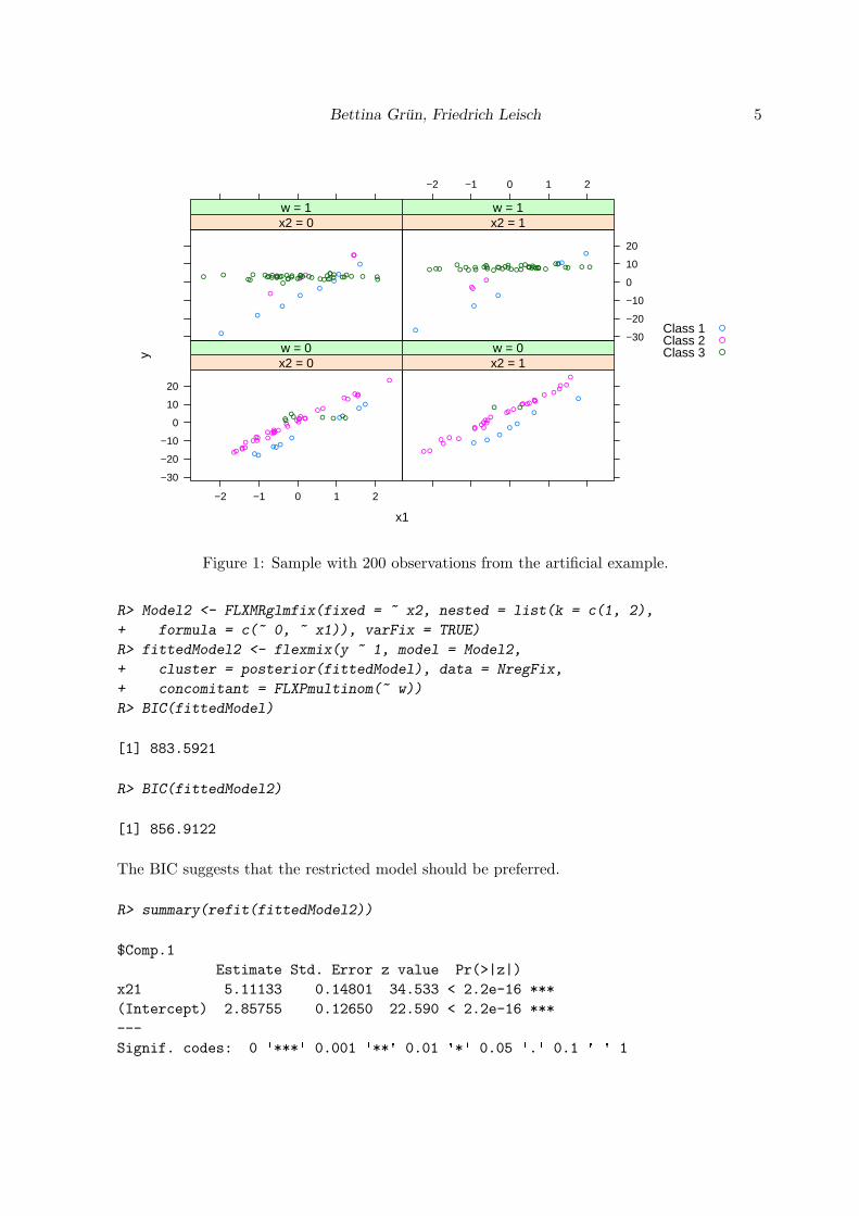
This artificial dataset with 200 observations is given in Grun and Leisch (2006). The data isgenerated from a mixture of Gaussian regression models with three components. There is anintercept with varying effects, an independent variable x1, which is a numeric variable, withfixed effects and another independent variable x2, which is a categorical variable with twolevels, with nested effects. The prior probabilities depend on a concomitant variable w, whichis also a categorical variable with two levels. Fixed effects are also assumed for the variance.The data is illustrated in Figure 1 and the true underlying model is given by:

H(y | (x1, x2), w,Θ) =S∑

s=1

πs(w,α)N(y |µs, σ2),

with βs = (βsIntercept, β

c(s)x1 , βx2). The nesting signifies that c(1) = c(2) and β

c(3)x1 = 0.


The mixture model is fitted by first loading the package and the dataset and then speci-fying the component specific model. In a first step a component specific model with onlyvarying effects is specified. Then the fitting function flexmix() is called repeatedly usingstepFlexmix(). Finally, we order the components such that they are in ascending order withrespect to the coefficients of the variable x1.

R> set.seed(2807)

R> library("flexmix")

R> data("NregFix", package = "flexmix")

R> Model <- FLXMRglm(~ x2 + x1)

R> fittedModel <- stepFlexmix(y ~ 1, model = Model, nrep = 3, k = 3,

+ data = NregFix, concomitant = FLXPmultinom(~ w))

3 : * * *

R> fittedModel <- relabel(fittedModel, "model", "x1")

R> summary(refit(fittedModel))

$Comp.1

Estimate Std. Error z value Pr(>|z|)

(Intercept) 2.87046 0.13515 21.2394 <2e-16 ***

x21 5.10209 0.20849 24.4716 <2e-16 ***

x1 0.13348 0.10633 1.2553 0.2094

---

Signif. codes: 0 ✬***✬ 0.001 ✬**✬ 0.01 ✬*✬ 0.05 ✬.✬ 0.1 ✬ ✬ 1

$Comp.2


(Intercept) 0.99358 0.18130 5.4803 4.245e-08 ***

x21 5.28836 0.25232 20.9590 < 2.2e-16 ***

x1 9.89243 0.11778 83.9892 < 2.2e-16 ***

---

Signif. codes: 0 ✬***✬ 0.001 ✬**✬ 0.01 ✬*✬ 0.05 ✬.✬ 0.1 ✬ ✬ 1

$Comp.3


(Intercept) -7.64055 0.25163 -30.365 < 2.2e-16 ***

x21 4.65090 0.38102 12.207 < 2.2e-16 ***

x1 9.93667 0.16444 60.429 < 2.2e-16 ***

---

Signif. codes: 0 ✬***✬ 0.001 ✬**✬ 0.01 ✬*✬ 0.05 ✬.✬ 0.1 ✬ ✬ 1

The estimated coefficients indicate that the components differ for the intercept, but that theyare not significantly different for the coefficients of x2. For x1 the coefficient of the firstcomponent is not significantly different from zero and the confidence intervals for the othertwo components overlap. Therefore we fit a modified model, which is equivalent to the trueunderlying model. The previously fitted model is used for initializing the EM algorithm:


x1

y

−30

−20

−10

0

10

20

−2 −1 0 1 2

●

●

●

●

●

●

●●

●

●●

●

●

●

●●

●

●●

●

●

●●

●

●

●

●●

●

●

●

●●

●

●

●●

●

●

●●

●

●

●

●●● ●● ●●

●

x2 = 0w = 0

●

●

●●

●

●

●

●●

●

●

●●

●

●

●

●

●

●

●●

●

●

●

●

●

●

●

●

●

●

●

●

●

●

●

●

●● ●

x2 = 1w = 0

●

●

●

●

●

●

●

●

●●

●

●● ● ●●

●●● ● ●●●

● ● ●● ● ●● ● ●●● ●●

●●

● ● ●● ● ●

● ●●●●● ●●● ●

●

●●

x2 = 0w = 1

−2 −1 0 1 2

−30

−20

−10

0

10

20

●

●

●

●

●

●

●

●●

●● ●● ●●● ●● ● ●●

●● ●●● ●● ● ●

●● ●●

●●●●●

● ● ●●●

●●● ● ●●●

x2 = 1w = 1

Class 1Class 2Class 3

●

●

●

Figure 1: Sample with 200 observations from the artificial example.

R> Model2 <- FLXMRglmfix(fixed = ~ x2, nested = list(k = c(1, 2),

+ formula = c(~ 0, ~ x1)), varFix = TRUE)

R> fittedModel2 <- flexmix(y ~ 1, model = Model2,

+ cluster = posterior(fittedModel), data = NregFix,

+ concomitant = FLXPmultinom(~ w))

R> BIC(fittedModel)

[1] 883.5921

R> BIC(fittedModel2)

[1] 856.9122

The BIC suggests that the restricted model should be preferred.

R> summary(refit(fittedModel2))

$Comp.1


x21 5.11133 0.14801 34.533 < 2.2e-16 ***

(Intercept) 2.85755 0.12650 22.590 < 2.2e-16 ***

---

Signif. codes: 0 ✬***✬ 0.001 ✬**✬ 0.01 ✬*✬ 0.05 ✬.✬ 0.1 ✬ ✬ 1


$Comp.2


x21 5.111327 0.148011 34.5334 < 2.2e-16 ***

x1 9.902341 0.091179 108.6027 < 2.2e-16 ***

(Intercept) 1.072193 0.141877 7.5572 4.119e-14 ***

---

Signif. codes: 0 ✬***✬ 0.001 ✬**✬ 0.01 ✬*✬ 0.05 ✬.✬ 0.1 ✬ ✬ 1

$Comp.3


x21 5.111327 0.148011 34.533 < 2.2e-16 ***

x1 9.902341 0.091179 108.603 < 2.2e-16 ***

(Intercept) -7.848359 0.197759 -39.687 < 2.2e-16 ***

---

Signif. codes: 0 ✬***✬ 0.001 ✬**✬ 0.01 ✬*✬ 0.05 ✬.✬ 0.1 ✬ ✬ 1

The coefficients are ordered such that the fixed coefficients are first, the nested varying coef-ficients second and the varying coefficients last.

3.2. Finite mixtures of binomial logit regressions

Beta blockers

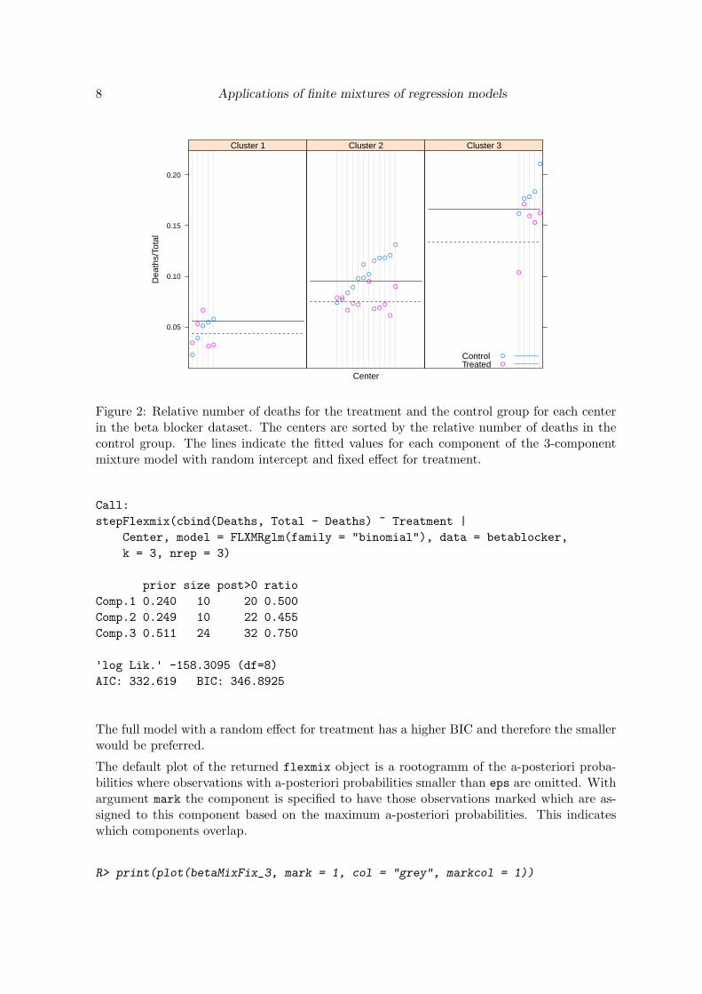
The dataset is analyzed in Aitkin (1999a,b) using a finite mixture of binomial regression mod-els. Furthermore, it is described in McLachlan and Peel (2000) on page 165. The dataset isfrom a 22-center clinical trial of beta-blockers for reducing mortality after myocardial infarc-tion. A two-level model is assumed to represent the data, where centers are at the upper leveland patients at the lower level. The data is illustrated in Figure 2 and the model is given by:

H(Deaths |Total,Treatment,Center,Θ) =

S∑

s=1

πsBi(Deaths |Total, θs).

First, the center classification is ignored and a binomial logit regression model with treatmentas covariate is fitted using glm, i.e. S = 1:

R> data("betablocker", package = "flexmix")

R> betaGlm <- glm(cbind(Deaths, Total - Deaths) ~ Treatment,

+ family = "binomial", data = betablocker)

R> betaGlm

Call: glm(formula = cbind(Deaths, Total - Deaths) ~ Treatment, family = "binomial",

data = betablocker)

Coefficients:

(Intercept) TreatmentTreated

-2.1971 -0.2574


Degrees of Freedom: 43 Total (i.e. Null); 42 Residual

Null Deviance: 333

Residual Deviance: 305.8 AIC: 527.2

In the next step the center classification is included by allowing a random effect for theintercept given the centers, i.e. the coefficients βs are given by (βs

Intercept|Center, βTreatment).This signifies that the component membership is fixed for each center. In order to determinethe suitable number of components, the mixture is fitted with different numbers of componentsand the BIC information criterion is used to select an appropriate model. In this case a modelwith three components is selected. The fitted values for the model with three components aregiven in Figure 2.

R> betaMixFix <- stepFlexmix(cbind(Deaths, Total - Deaths) ~ 1 | Center,

+ model = FLXMRglmfix(family = "binomial", fixed = ~ Treatment),

+ k = 2:4, nrep = 3, data = betablocker)

2 : * * *

3 : * * *

4 : * * *

R> betaMixFix

Call:

stepFlexmix(cbind(Deaths, Total - Deaths) ~ 1 | Center,

model = FLXMRglmfix(family = "binomial", fixed = ~Treatment),

data = betablocker, k = 2:4, nrep = 3)

iter converged k k0 logLik AIC BIC ICL

2 12 TRUE 2 2 -181.3308 370.6617 377.7984 380.2114

3 9 TRUE 3 3 -159.3605 330.7210 341.4262 343.3249

4 15 TRUE 4 4 -155.7540 327.5080 341.7815 345.7338

In addition the treatment effect can also be included in the random part of the model. Asthen all coefficients for the covariates and the intercept follow a mixture distribution thecomponent specific model can be specified using FLXMRglm(). The coefficients are βs =(βs

Intercept|Center, βsTreatment|Center), i.e. it is assumed that the heterogeneity is only between

centers and therefore the aggregated data for each center can be used.

R> betaMix <- stepFlexmix(cbind(Deaths, Total - Deaths) ~ Treatment | Center,

+ model = FLXMRglm(family = "binomial"), k = 3, nrep = 3,

+ data = betablocker)

3 : * * *

R> summary(betaMix)


Center

Dea

ths/

Tota

l

0.05

0.10

0.15

0.20

●●

●

●

●

●

●

●

● ●

Cluster 1

●

●●

●

●

●

●

●

●

●

●

●

●

●

●

●

●

●

●●

●●

●

●

Cluster 2

●

●

●

●●

●

●

●●

●

Cluster 3

ControlTreated

●

●

Figure 2: Relative number of deaths for the treatment and the control group for each centerin the beta blocker dataset. The centers are sorted by the relative number of deaths in thecontrol group. The lines indicate the fitted values for each component of the 3-componentmixture model with random intercept and fixed effect for treatment.

Call:

stepFlexmix(cbind(Deaths, Total - Deaths) ~ Treatment |

Center, model = FLXMRglm(family = "binomial"), data = betablocker,

k = 3, nrep = 3)

prior size post>0 ratio

Comp.1 0.240 10 20 0.500

Comp.2 0.249 10 22 0.455

Comp.3 0.511 24 32 0.750

✬log Lik.✬ -158.3095 (df=8)

AIC: 332.619 BIC: 346.8925

The full model with a random effect for treatment has a higher BIC and therefore the smallerwould be preferred.

The default plot of the returned flexmix object is a rootogramm of the a-posteriori proba-bilities where observations with a-posteriori probabilities smaller than eps are omitted. Withargument mark the component is specified to have those observations marked which are as-signed to this component based on the maximum a-posteriori probabilities. This indicateswhich components overlap.

R> print(plot(betaMixFix_3, mark = 1, col = "grey", markcol = 1))


Rootogram of posterior probabilities > 1e−04

0.0

1.5

3.0

4.5

6.0

7.5

9.0

0.0 0.2 0.4 0.6 0.8 1.0

Comp. 1

0.0 0.2 0.4 0.6 0.8 1.0

Comp. 2

0.0 0.2 0.4 0.6 0.8 1.0

Comp. 3

The default plot of the fitted model indicates that the components are well separated. Inaddition component 1 has a slight overlap with component 2 but none with component 3.

The fitted parameters of the component specific models can be accessed with:

R> parameters(betaMix)

Comp.1 Comp.2 Comp.3

coef.(Intercept) -2.91633602 -1.5800104 -2.2476996

coef.TreatmentTreated -0.08047852 -0.3248495 -0.2630025

The cluster assignments using the maximum a-posteriori probabilities are obtained with:

R> table(clusters(betaMix))

1 2 3

10 10 24

The estimated probabilities for each component for the treated patients and those in thecontrol group can be obtained with:

R> predict(betaMix,

+ newdata = data.frame(Treatment = c("Control", "Treated")))

$Comp.1

[,1]

1 0.05135190

2 0.04756999

$Comp.2

[,1]


1 0.1707940

2 0.1295594

$Comp.3

[,1]

1 0.09554808

2 0.07511132

or

R> fitted(betaMix)[c(1, 23), ]

Comp.1 Comp.2 Comp.3

[1,] 0.05135190 0.1707940 0.09554808

[2,] 0.04756999 0.1295594 0.07511132

A further analysis of the model is possible with function refit() which returns the estimatedcoefficients together with the standard deviations, z-values and corresponding p-values:

R> summary(refit(getModel(betaMixFix, "3")))

$Comp.1


TreatmentTreated -0.258163 0.049901 -5.1735 2.297e-07 ***

(Intercept) -2.250160 0.040529 -55.5204 < 2.2e-16 ***

---

Signif. codes: 0 ✬***✬ 0.001 ✬**✬ 0.01 ✬*✬ 0.05 ✬.✬ 0.1 ✬ ✬ 1

$Comp.2



(Intercept) -2.833679 0.075079 -37.7428 < 2.2e-16 ***

---

Signif. codes: 0 ✬***✬ 0.001 ✬**✬ 0.01 ✬*✬ 0.05 ✬.✬ 0.1 ✬ ✬ 1

$Comp.3



(Intercept) -1.609726 0.055735 -28.8819 < 2.2e-16 ***

---

Signif. codes: 0 ✬***✬ 0.001 ✬**✬ 0.01 ✬*✬ 0.05 ✬.✬ 0.1 ✬ ✬ 1

The printed coefficients are ordered to have the fixed effects before the varying effects.

Mehta et al. trial

This dataset is similar to the beta blocker dataset and is also analyzed in Aitkin (1999b).The dataset is visualized in Figure 3. The observation for the control group in center 15 isslightly conspicuous and might classify as an outlier.


The model is given by:

H(Response |Total,Θ) =

S∑

s=1

πsBi(Response |Total, θs),

with βs = (βsIntercept|Site, βDrug). This model is fitted with:

R> data("Mehta", package = "flexmix")

R> mehtaMix <- stepFlexmix(cbind(Response, Total - Response)~ 1 | Site,

+ model = FLXMRglmfix(family = "binomial", fixed = ~ Drug),

+ control = list(minprior = 0.04), nrep = 3, k = 3, data = Mehta)

3 : * * *

R> summary(mehtaMix)

Call:

stepFlexmix(cbind(Response, Total - Response) ~ 1 | Site,

model = FLXMRglmfix(family = "binomial", fixed = ~Drug),

control = list(minprior = 0.04), data = Mehta, k = 3,

nrep = 3)


Comp.1 0.0456 2 4 0.500

Comp.2 0.5012 22 44 0.500

Comp.3 0.4532 20 42 0.476

✬log Lik.✬ -66.8056 (df=6)

AIC: 145.6112 BIC: 156.3163

One component only contains the observations for center 15 and in order to be able to fita mixture with such a small component it is necessary to modify the default argument forminprior which is 0.05. The fitted values for this model are given separately for each com-ponent in Figure 3.

If also a random effect for the coefficient of Drug is fitted, i.e. βs = (βsIntercept|Site, β

sDrug|Site),

this is estimated by:

R> mehtaMix <- stepFlexmix(cbind(Response, Total - Response) ~ Drug | Site,

+ model = FLXMRglm(family = "binomial"), k = 3, data = Mehta, nrep = 3,

+ control = list(minprior = 0.04))

3 : * * *



Site

Res

pons

e/To

tal

0.0

0.2

0.4

0.6

0.8

●

●

Cluster 1

●

●●

●

●

●

●

●

● ●

● ●●

●●

●

●

●

●

●

●

●

Cluster 2

●

●

●●● ●●

● ●●● ●

●●

● ●●

● ●

●

Cluster 3

NewControl

●

●

Figure 3: Relative number of responses for the treatment and the control group for each sitein the Mehta et al. trial dataset together with the fitted values. The sites are sorted by therelative number of responses in the control group.

Call:

stepFlexmix(cbind(Response, Total - Response) ~ Drug |

Site, model = FLXMRglm(family = "binomial"), data = Mehta,

control = list(minprior = 0.04), k = 3, nrep = 3)


Comp.1 0.5084 22 42 0.524

Comp.2 0.0455 2 2 1.000

Comp.3 0.4462 20 42 0.476

✬log Lik.✬ -62.02723 (df=8)

AIC: 140.0545 BIC: 154.328

The BIC is smaller for the larger model and this indicates that the assumption of an equaldrug effect for all centers is not confirmed by the data.

Given Figure 3 a two-component model with fixed treatment is also fitted to the data wheresite 15 is omitted:

R> Mehta.sub <- subset(Mehta, Site != 15)

R> mehtaMix <- stepFlexmix(cbind(Response, Total - Response) ~ 1 | Site,

+ model = FLXMRglmfix(family = "binomial", fixed = ~ Drug),

+ data = Mehta.sub, k = 2, nrep = 3)

2 : * * *



Call:

stepFlexmix(cbind(Response, Total - Response) ~ 1 | Site,

model = FLXMRglmfix(family = "binomial", fixed = ~Drug),

data = Mehta.sub, k = 2, nrep = 3)


Comp.1 0.472 20 42 0.476

Comp.2 0.528 22 42 0.524

✬log Lik.✬ -56.5844 (df=4)

AIC: 121.1688 BIC: 128.1195

Tribolium

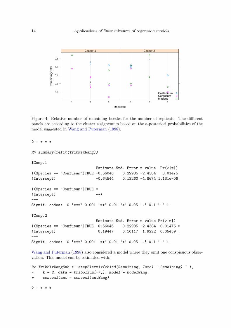
A finite mixture of binomial regressions is fitted to the Tribolium dataset given in Wang andPuterman (1998). The data was collected to investigate whether the adult Tribolium speciesCastaneum has developed an evolutionary advantage to recognize and avoid eggs of its ownspecies while foraging, as beetles of the genus Tribolium are cannibalistic in the sense thatadults eat the eggs of their own species as well as those of closely related species.

The experiment isolated a number of adult beetles of the same species and presented themwith a vial of 150 eggs (50 of each type), the eggs being thoroughly mixed to ensure uniformitythroughout the vial. The data gives the consumption data for adult Castaneum species. Itreports the number of Castaneum, Confusum and Madens eggs, respectively, that remainuneaten after two day exposure to the adult beetles. Replicates 1, 2, and 3 correspond todifferent occasions on which the experiment was conducted. The data is visualized in Figure 4and the model is given by:

H(Remaining |Total,Θ) =

S∑

s=1

πs(Replicate,α)Bi(Remaining |Total, θs),

with βs = (βsIntercept,βSpecies). This model is fitted with:

R> data("tribolium", package = "flexmix")

R> TribMix <- stepFlexmix(cbind(Remaining, Total - Remaining) ~ 1,

+ k = 2:3, model = FLXMRglmfix(fixed = ~ Species, family = "binomial"),

+ concomitant = FLXPmultinom(~ Replicate), data = tribolium)

2 : * * *

3 : * * *

The model which is selected as the best in Wang and Puterman (1998) can be estimated with:

R> modelWang <- FLXMRglmfix(fixed = ~ I(Species == "Confusum"),

+ family = "binomial")

R> concomitantWang <- FLXPmultinom(~ I(Replicate == 3))

R> TribMixWang <- stepFlexmix(cbind(Remaining, Total - Remaining) ~ 1,

+ data = tribolium, model = modelWang, concomitant = concomitantWang,

+ k = 2)


Replicate

Rem

aini

ng/T

otal

0.2

0.3

0.4

0.5

0.6

1 2 3

●●

●

●

●

●●

●

●

●

●

●●

●

Cluster 1

1 2 3

●●●

●

●

●

●

●

●

●

●

●

●

Cluster 2

CastaneumConfusumMadens

●

●

●

Figure 4: Relative number of remaining beetles for the number of replicate. The differentpanels are according to the cluster assignemnts based on the a-posteriori probabilities of themodel suggested in Wang and Puterman (1998).

2 : * * *

R> summary(refit(TribMixWang))

$Comp.1


I(Species == "Confusum")TRUE -0.56046 0.22985 -2.4384 0.01475

(Intercept) -0.64544 0.13260 -4.8674 1.131e-06

I(Species == "Confusum")TRUE *

(Intercept) ***

---

Signif. codes: 0 ✬***✬ 0.001 ✬**✬ 0.01 ✬*✬ 0.05 ✬.✬ 0.1 ✬ ✬ 1

$Comp.2


I(Species == "Confusum")TRUE -0.56046 0.22985 -2.4384 0.01475 *

(Intercept) 0.19447 0.10117 1.9222 0.05459 .

---

Signif. codes: 0 ✬***✬ 0.001 ✬**✬ 0.01 ✬*✬ 0.05 ✬.✬ 0.1 ✬ ✬ 1

Wang and Puterman (1998) also considered a model where they omit one conspicuous obser-vation. This model can be estimated with:

R> TribMixWangSub <- stepFlexmix(cbind(Remaining, Total - Remaining) ~ 1,

+ k = 2, data = tribolium[-7,], model = modelWang,

+ concomitant = concomitantWang)

2 : * * *


Trypanosome

The data is used in Follmann and Lambert (1989). It is from a dosage-response analysiswhere the proportion of organisms belonging to different populations shall be assessed. It isassumed that organisms belonging to different populations are indistinguishable other thanin terms of their reaction to the stimulus. The experimental technique involved inspectionunder the microscope of a representative aliquot of a suspension, all organisms appearingwithin two fields of view being classified either alive or dead. Hence the total numbers oforganisms present at each dose and the number showing the quantal response were bothrandom variables. The data is illustrated in Figure 5.

The model which is proposed in Follmann and Lambert (1989) is given by:

H(Dead |Θ) =

S∑

s=1

πsBi(Dead | θs),

where Dead ∈ {0, 1} and with βs = (βsIntercept,βlog(Dose)). This model is fitted with:

R> data("trypanosome", package = "flexmix")

R> TrypMix <- stepFlexmix(cbind(Dead, 1-Dead) ~ 1, k = 2, nrep = 3,

+ data = trypanosome, model = FLXMRglmfix(family = "binomial",

+ fixed = ~ log(Dose)))

2 : * * *

R> summary(refit(TrypMix))

$Comp.1


log(Dose) 124.895 25.261 4.9442 7.645e-07 ***

(Intercept) -196.324 39.591 -4.9588 7.091e-07 ***

---

Signif. codes: 0 ✬***✬ 0.001 ✬**✬ 0.01 ✬*✬ 0.05 ✬.✬ 0.1 ✬ ✬ 1

$Comp.2


log(Dose) 124.895 25.261 4.9442 7.645e-07 ***

(Intercept) -205.864 41.802 -4.9248 8.446e-07 ***

---

Signif. codes: 0 ✬***✬ 0.001 ✬**✬ 0.01 ✬*✬ 0.05 ✬.✬ 0.1 ✬ ✬ 1

The fitted values are given in Figure 5 together with the fitted values of a generalized linearmodel in order to facilitate comparison of the two models.

3.3. Finite mixtures of Poisson regressions

Fabric faults

The dataset is analyzed using a finite mixture of Poisson regression models in Aitkin (1996).Furthermore, it is described in McLachlan and Peel (2000) on page 155. It contains 32


●

●

●●

●

●

●

●

4.7 4.8 4.9 5.0 5.1 5.2 5.3 5.4

0.0

0.2

0.4

0.6

0.8

1.0

Dose

Dea

d/(D

ead

+ A

live)

GLMMixture model

Figure 5: Relative number of deaths for each dose level together with the fitted values for thegeneralized linear model (“GLM”) and the random intercept model (“Mixture model”).

observations on the number of faults in rolls of a textile fabric. A random intercept model isused where a fixed effect is assumed for the logarithm of length:

R> data("fabricfault", package = "flexmix")

R> fabricMix <- stepFlexmix(Faults ~ 1, model = FLXMRglmfix(family="poisson",

+ fixed = ~ log(Length)), data = fabricfault, k = 2, nrep = 3)

2 : * * *

R> summary(fabricMix)

Call:

stepFlexmix(Faults ~ 1, model = FLXMRglmfix(family = "poisson",

fixed = ~log(Length)), data = fabricfault, k = 2,

nrep = 3)


Comp.1 0.796 27 32 0.844

Comp.2 0.204 5 32 0.156

✬log Lik.✬ -86.33119 (df=4)

AIC: 180.6624 BIC: 186.5253

R> summary(refit(fabricMix))

$Comp.1



log(Length) 0.79913 0.23491 3.4019 0.0006692 ***

(Intercept) -3.12797 1.51934 -2.0588 0.0395167 *

---

Signif. codes: 0 ✬***✬ 0.001 ✬**✬ 0.01 ✬*✬ 0.05 ✬.✬ 0.1 ✬ ✬ 1

$Comp.2


log(Length) 0.79913 0.23491 3.4019 0.0006692 ***

(Intercept) -2.36202 1.59146 -1.4842 0.1377594

---

Signif. codes: 0 ✬***✬ 0.001 ✬**✬ 0.01 ✬*✬ 0.05 ✬.✬ 0.1 ✬ ✬ 1

R> Lnew <- seq(0, 1000, by = 50)

R> fabricMix.pred <- predict(fabricMix, newdata = data.frame(Length = Lnew))

The intercept of the first component is not significantly different from zero for a signficancelevel of 0.05. We therefore also fit a modified model where the intercept is a-priori set to zerofor the first component. This nested structure is given as part of the model specification withargument nested.

R> fabricMix2 <- flexmix(Faults ~ 0, data = fabricfault,

+ cluster = posterior(fabricMix),

+ model = FLXMRglmfix(family = "poisson", fixed = ~ log(Length),

+ nested = list(k=c(1,1), formula=list(~0,~1))))

R> summary(refit(fabricMix2))

$Comp.1


log(Length) 0.308000 0.013437 22.922 < 2.2e-16 ***

---

Signif. codes: 0 ✬***✬ 0.001 ✬**✬ 0.01 ✬*✬ 0.05 ✬.✬ 0.1 ✬ ✬ 1

$Comp.2


log(Length) 0.308000 0.013437 22.9215 < 2.2e-16 ***

(Intercept) 0.921282 0.132720 6.9415 3.878e-12 ***

---

Signif. codes: 0 ✬***✬ 0.001 ✬**✬ 0.01 ✬*✬ 0.05 ✬.✬ 0.1 ✬ ✬ 1

R> fabricMix2.pred <- predict(fabricMix2,

+ newdata = data.frame(Length = Lnew))

The data and the fitted values for each of the components for both models are given inFigure 6.

Patent

The patent data given in Wang, Cockburn, and Puterman (1998) consist of 70 observationson patent applications, R&D spending and sales in millions of dollar from pharmaceutical and


●

●

●

●

●

●

●

●●●●

●

●

●

●

●

●●

●

●

●

●

●

●

●

●

●

●

●

●

●

●

200 400 600 800

05

1015

2025

Length

Faul

ts

Model 1Model 2

Figure 6: Observed values of the fabric faults dataset together with the fitted values for thecomponents of each of the two fitted models.

biomedical companies in 1976 taken from the National Bureau of Economic Research R&DMasterfile. The observations are displayed in Figure 7. The model which is chosen as thebest in Wang et al. (1998) is given by:

H(Patents | lgRD,RDS,Θ) =

S∑

s=1

πs(RDS,α)Poi(Patents |λs),

and βs = (βsIntercept, β

slgRD).

The model is fitted with:

R> data("patent", package = "flexmix")

R> ModelPat <- FLXMRglm(family = "poisson")

R> FittedPat <- stepFlexmix(Patents ~ lgRD, k = 3, nrep = 3,

+ model = ModelPat, data = patent, concomitant = FLXPmultinom(~ RDS))

3 : * * *

R> summary(FittedPat)

Call:

stepFlexmix(Patents ~ lgRD, model = ModelPat, data = patent,

concomitant = FLXPmultinom(~RDS), k = 3, nrep = 3)


Comp.1 0.615 45 63 0.714

Comp.2 0.184 13 47 0.277


Comp.3 0.201 12 48 0.250

✬log Lik.✬ -197.6753 (df=10)

AIC: 415.3506 BIC: 437.8355

The fitted values for the component specific models and the concomitant variable modelare given in Figure 7. The plotting symbol of the observations corresponds to the inducedclustering given by clusters(FittedPat).

This model is modified to have fixed effects for the logarithmized R&D spendings, i.e. (β)s =(βs

Intercept, βlgRD). The already fitted model is used for initialization, i.e. the EM algorithm isstarted with an M-step given the a-posteriori probabilities.

R> ModelFixed <- FLXMRglmfix(family = "poisson", fixed = ~ lgRD)

R> FittedPatFixed <- flexmix(Patents ~ 1, model = ModelFixed,

+ cluster = posterior(FittedPat), concomitant = FLXPmultinom(~ RDS),

+ data = patent)

R> summary(FittedPatFixed)

Call:

flexmix(formula = Patents ~ 1, data = patent, cluster = posterior(FittedPat),

model = ModelFixed, concomitant = FLXPmultinom(~RDS))


Comp.1 0.361 25 63 0.397

Comp.2 0.203 14 52 0.269

Comp.3 0.436 31 54 0.574

✬log Lik.✬ -216.824 (df=8)

AIC: 449.6479 BIC: 467.6359

The fitted values for the component specific models and the concomitant variable model ofthis model are also given in Figure 7.

With respect to the BIC the full model is better than the model with the fixed effects.However, fixed effects have the advantage that the different components differ only in theirbaseline and the relation between the components in return of investment for each additionalunit of R&D spending is constant. Due to a-priori domain knowledge this model might seemmore plausible. The fitted values for the constrained model are also given in Figure 7.

Seizure

The data is used in Wang, Puterman, Cockburn, and Le (1996) and is from a clinical trialwhere the effect of intravenous gamma-globulin on suppression of epileptic seizures is studied.There are daily observations for a period of 140 days on one patient, where the first 27 daysare a baseline period without treatment, the remaining 113 days are the treatment period.The model proposed in Wang et al. (1996) is given by:

H(Seizures | (Treatment, log(Day), log(Hours)),Θ) =

S∑

s=1

πsPoi(Seizures |λs),


log(R&D)

Pat

ents 0

50

100

150

200

● ● ●

●

●

●●

●

●

●

● ●●● ●● ●● ●●

●

● ●

●

●● ●●●

●

●● ●

●

●●●

●●●

●

●●

●●

●

●

●● ●●

●

●

●

●

●●

●

●

● ●● ●● ●● ●

●

● ●

Wang et al.

0

50

100

150

200

−2 0 2 4

● ●

●

●

●●

●

●

● ●● ●●● ● ●

●

●●

●

● ●

●

●●

●

●

●● ●●

●

●●

●

●

●●

●

●

●● ●● ● ●●● ●●●●

●

● ●●●●●● ●●● ●

●●●

●●

●

Fixed effects

RDS

Pro

babi

lity

0.0

0.2

0.4

0.6

0.8

Wang et al.

0.0

0.2

0.4

0.6

0.8

0.0 0.5 1.0 1.5 2.0 2.5 3.0

Fixed effects

Figure 7: Patent data with the fitted values of the component specific models (left) and theconcomitant variable model (right) for the model in Wang et al. and with fixed effects forlog(R&D). The plotting symbol for each observation is determined by the component withthe maximum a-posteriori probability.


where (β)s = (βsIntercept, β

sTreatment, β

slog(Day), β

sTreatment:log(Day)) and log(Hours) is used as off-

set. This model is fitted with:

R> data("seizure", package = "flexmix")

R> seizMix <- stepFlexmix(Seizures ~ Treatment * log(Day), data = seizure,

+ k = 2, nrep = 3, model = FLXMRglm(family = "poisson",

+ offset = log(seizure$Hours)))

2 : * * *

R> summary(seizMix)

Call:

stepFlexmix(Seizures ~ Treatment * log(Day), data = seizure,

model = FLXMRglm(family = "poisson", offset = log(seizure$Hours)),

k = 2, nrep = 3)


Comp.1 0.724 103 115 0.896

Comp.2 0.276 37 101 0.366

✬log Lik.✬ -376.1762 (df=9)

AIC: 770.3525 BIC: 796.8272

R> summary(refit(seizMix))

$Comp.1


(Intercept) 2.070226 0.092252 22.441 < 2.2e-16 ***

TreatmentYes 7.432200 0.548865 13.541 < 2.2e-16 ***

log(Day) -0.270550 0.042320 -6.393 1.626e-10 ***

TreatmentYes:log(Day) -2.276359 0.147857 -15.396 < 2.2e-16 ***

---

Signif. codes: 0 ✬***✬ 0.001 ✬**✬ 0.01 ✬*✬ 0.05 ✬.✬ 0.1 ✬ ✬ 1

$Comp.2


(Intercept) 2.84422 0.25898 10.9825 < 2.2e-16 ***

TreatmentYes 1.30319 0.54448 2.3935 0.016690 *

log(Day) -0.40593 0.10014 -4.0537 5.04e-05 ***

TreatmentYes:log(Day) -0.43139 0.15265 -2.8261 0.004712 **

---

Signif. codes: 0 ✬***✬ 0.001 ✬**✬ 0.01 ✬*✬ 0.05 ✬.✬ 0.1 ✬ ✬ 1

A different model with different contrasts to directly estimate the coefficients for the jumpwhen changing between base and treatment period is given by:


R> seizMix2 <- flexmix(Seizures ~ Treatment * log(Day/27),

+ data = seizure, cluster = posterior(seizMix),

+ model = FLXMRglm(family = "poisson", offset = log(seizure$Hours)))

R> summary(seizMix2)

Call:

flexmix(formula = Seizures ~ Treatment * log(Day/27),

data = seizure, cluster = posterior(seizMix), model = FLXMRglm(family = "poisson",

offset = log(seizure$Hours)))


Comp.1 0.724 103 115 0.896

Comp.2 0.276 37 101 0.366

✬log Lik.✬ -376.1762 (df=9)

AIC: 770.3524 BIC: 796.8272

R> summary(refit(seizMix2))

$Comp.1


(Intercept) 1.178452 0.072453 16.2650 < 2.2e-16 ***

TreatmentYes -0.070116 0.116887 -0.5999 0.5486

log(Day/27) -0.270600 0.042324 -6.3935 1.621e-10 ***

TreatmentYes:log(Day/27) -2.276249 0.147854 -15.3953 < 2.2e-16 ***

---

Signif. codes: 0 ✬***✬ 0.001 ✬**✬ 0.01 ✬*✬ 0.05 ✬.✬ 0.1 ✬ ✬ 1

$Comp.2


(Intercept) 1.506044 0.091612 16.4394 < 2.2e-16 ***

TreatmentYes -0.118471 0.140926 -0.8407 0.40054

log(Day/27) -0.406176 0.100100 -4.0577 4.956e-05 ***

TreatmentYes:log(Day/27) -0.431134 0.152620 -2.8249 0.00473 **

---

Signif. codes: 0 ✬***✬ 0.001 ✬**✬ 0.01 ✬*✬ 0.05 ✬.✬ 0.1 ✬ ✬ 1

A different model which allows no jump at the change between base and treatment period isfitted with:

R> seizMix3 <- flexmix(Seizures ~ log(Day/27)/Treatment, data = seizure,

+ cluster = posterior(seizMix), model = FLXMRglm(family = "poisson",

+ offset = log(seizure$Hours)))

R> summary(seizMix3)

Call:

flexmix(formula = Seizures ~ log(Day/27)/Treatment, data = seizure,


cluster = posterior(seizMix), model = FLXMRglm(family = "poisson",

offset = log(seizure$Hours)))


Comp.1 0.722 102 115 0.887

Comp.2 0.278 38 101 0.376

✬log Lik.✬ -376.6495 (df=7)

AIC: 767.2991 BIC: 787.8906

R> summary(refit(seizMix3))

$Comp.1


(Intercept) 1.150003 0.058217 19.7537 < 2.2e-16 ***

log(Day/27) -0.283878 0.036969 -7.6788 1.606e-14 ***

log(Day/27):TreatmentYes -2.311510 0.134828 -17.1441 < 2.2e-16 ***

---

Signif. codes: 0 ✬***✬ 0.001 ✬**✬ 0.01 ✬*✬ 0.05 ✬.✬ 0.1 ✬ ✬ 1

$Comp.2


(Intercept) 1.458918 0.067241 21.6968 < 2.2e-16 ***

log(Day/27) -0.447634 0.081633 -5.4835 4.17e-08 ***

log(Day/27):TreatmentYes -0.458721 0.145578 -3.1510 0.001627 **

---

Signif. codes: 0 ✬***✬ 0.001 ✬**✬ 0.01 ✬*✬ 0.05 ✬.✬ 0.1 ✬ ✬ 1

With respect to the BIC criterion the smaller model with no jump is preferred. This is also themore intuitive model from a practitioner’s point of view, as it does not seem to be plausiblethat starting the treatment already gives a significant improvement, but improvement developsover time. The data points together with the fitted values for each component of the twomodels are given in Figure 8. It can clearly be seen that the fitted values are nearly equalwhich also supports the smaller model.

Ames salmonella assay data

The ames salomnella assay dataset was used in Wang et al. (1996). They propose a modelgiven by:

H(y | x,Θ) =S∑

s=1

πsPoi(y |λs),

where βs = (βsIntercept, βx, βlog(x+10)). The model is fitted with:

R> data("salmonellaTA98", package = "flexmix")

R> salmonMix <- stepFlexmix(y ~ 1, data = salmonellaTA98, k = 2, nrep = 3,

+ model = FLXMRglmfix(family = "poisson", fixed = ~ x + log(x + 10)))


●●

●

●●

●

●

●

●

●●

●

●

●

●

●

●●●

●●

●

●●

●

●

●

0 20 40 60 80 100 120 140

02

46

8

Day

Sei

zure

s/H

ours

● BaselineTreatment

Model 1Model 3

Figure 8: Observed values for the seizure dataset together with the fitted values for thecomponents of the two different models.

2 : * * *

4. Conclusions and future work

Package flexmix can be used to fit finite mixtures of regressions to datasets used in theliterature to illustrate these models. The results can be reproduced and additional insightscan be gained using visualization methods available in R. The fitted model is an object in R

which can be explored using show(), summary() or plot(), as suitable methods have beenimplemented for objects of class "flexmix" which are returned by flexmix().

In the future it would be desirable to have more diagnostic tools available to analyze the modelfit and compare different models. The use of resampling methods would be convenient as theycan be applied to all kinds of mixtures models and would therefore suit well the purpose ofthe package which is flexible modelling of various finite mixture models. Furthermore, anadditional visualization method for the fitted coefficients of the mixture would facilitate thecomparison of the components.

Computational details

All computations and graphics in this paper have been done using R version 3.3.3 with thepackages mvtnorm 1.0-6, ellipse 0.3-8, diptest 0.75-7, flexmix 2.3-14, lattice 0.20-35, model-

tools 0.2-21, tools 3.3.3, nnet 7.3-12, stats4 3.3.3.


2

2

1

222

2

2

2

2

2

1

2

22

2

2

1

0 200 400 600 800 1000

2030

4050

60

Dose of quinoline

Num

ber

of r

ever

tant

col

onie

s of

sal

mon

ella

Figure 9: Means and classification for assay data according to the estimated posterior prob-abilities based on the fitted model.

Acknowledgments

This research was supported by the the Austrian Science Foundation (FWF) under grantP17382 and the Austrian Academy of Sciences (OAW) through a DOC-FFORTE scholarshipfor Bettina Grun.

References

Aitkin M (1996). “A General Maximum Likelihood Analysis of Overdispersion in GeneralizedLinear Models.” Statistics and Computing, 6, 251–262.

Aitkin M (1999a). “A General Maximum Likelihood Analysis of Variance Components inGeneralized Linear Models.” Biometrics, 55, 117–128.

Aitkin M (1999b). “Meta-Analysis by Random Effect Modelling in Generalized Linear Mod-els.” Statistics in Medicine, 18(17–18), 2343–2351.

Follmann DA, Lambert D (1989). “Generalizing Logistic Regression by Non-Parametric Mix-ing.” Journal of the American Statistical Association, 84(405), 295–300.

Fraley C, Raftery AE (2002). “MCLUST: Software for Model-Based Clustering, DiscriminantAnalysis and Density Estimation.” Technical Report 415, Department of Statistics, Univer-sity of Washington, Seattle, WA, USA. URL http://www.stat.washington.edu/raftery.

Grun B, Leisch F (2006). “Fitting Finite Mixtures of Linear Regression Models with Varying& Fixed Effects in R.” In A Rizzi, M Vichi (eds.), Compstat 2006—Proceedings in Compu-

tational Statistics, pp. 853–860. Physica Verlag, Heidelberg, Germany. ISBN 3-7908-1708-2.

http://www.stat.washington.edu/raftery


Leisch F (2004). “FlexMix: A General Framework for Finite Mixture Models and Latent ClassRegression in R.” Journal of Statistical Software, 11(8). URL http://www.jstatsoft.

org/v11/i08/.

McLachlan G, Peel D (2000). Finite Mixture Models. John Wiley and Sons Inc.

Venables WN, Ripley BD (2002). Modern Applied Statistics with S. Fourth edition. SpringerVerlag, New York. ISBN 0-387-95457-0.

Wang P, Cockburn IM, Puterman ML (1998). “Analysis of Patent Data—A Mixed-Poisson-Regression-Model Approach.” Journal of Business & Economic Statistics, 16(1), 27–41.

Wang P, Puterman ML (1998). “Mixed Logistic Regression Models.” Journal of Agricultural,

Biological, and Environmental Statistics, 3(2), 175–200.

Wang P, Puterman ML, Cockburn IM, Le ND (1996). “Mixed Poisson Regression Modelswith Covariate Dependent Rates.” Biometrics, 52, 381–400.

Affiliation:

Bettina GrunInstitut fur Angewandte Statistik / IFASJohannes Kepler Universitat LinzFreistadter Straße 3154040 Linz, AustriaE-mail: [email protected]

Friedrich LeischInstitut fur Angewandte Statistik und EDVUniversitat fur Bodenkultur WienPeter Jordan Straße 821190 Wien, AustriaE-mail: [email protected]: http://www.statistik.lmu.de/~leisch/

http://www.jstatsoft.org/v11/i08/

http://www.jstatsoft.org/v11/i08/

mailto:[email protected]

mailto:[email protected]

http://www.statistik.lmu.de/~leisch/

applications of finite mixtures of regression models

Documents