1

Applications of Fat Tail Models

to Financial Markets Proposal

2/11/2014

Sudhalahari Bommareddy

Saad El Beleidy

Sujitreddy Narapareddy

Numan Yoner

Sponsor: Dr. Kuo Chu Chang

2

Contents Abstract ........................................................................................................................................... 3

Context ............................................................................................................................................ 3

Financial Engineering .................................................................................................................. 3

Financial Modeling Techniques .................................................................................................. 3

Problem Statement ......................................................................................................................... 5

Scope .............................................................................................................................................. 5

Technical Approach ........................................................................................................................ 5

General Data Analysis ................................................................................................................ 6

Whole Data Modeling .................................................................................................................. 6

t Distribution ............................................................................................................................. 7

Mixed Normal Distribution ....................................................................................................... 8

Extreme Scenario Modeling ........................................................................................................ 9

Generalized Extreme Value (GEV) Distribution .................................................................... 10

Generalized Pareto Distribution (GPD) ................................................................................. 10

Combined Whole Data & EVT Distribution ........................................................................... 11

Model Verification ...................................................................................................................... 11

Applications ............................................................................................................................... 11

Value at Risk (VaR) ............................................................................................................... 11

Option Pricing ........................................................................................................................ 11

Expected Results .......................................................................................................................... 11

Expected Model Results ........................................................................................................... 12

t-Distribution ........................................................................................................................... 12

Mixed Normal Distribution ..................................................................................................... 12

GEV and GPD Distributions .................................................................................................. 12

Expected Application Results ................................................................................................... 12

Project Plan ................................................................................................................................... 13

References .................................................................................................................................... 17

Appendix ....................................................................................................................................... 19

3

Abstract Normal distributions are commonly used in many modeling techniques to describe reality yet in

many cases, reality follows a fat-tailed distribution not a normal one. This critical assumption

results in potentially inaccurate models especially when modeling extreme events such as risk

or financial market changes. The aim of this project is to develop distribution models that more

accurately represent the reality of these extreme scenarios as well as apply this model in option

price and Value at Risk calculations.

Context

Financial Engineering Financial engineering is a multidisciplinary field that involves the use of mathematical

techniques and analyses to solve financial problems. It uses a variety of tools such as statistics,

concepts of economics, computer science, and applied mathematics to help address the

financial market, present and future. Financial engineering is primarily used as an analysis

technique for financial corporations such as corporate banks, hedge funds, and investment

banks.

A common factor in most of the definitions of Financial Engineering is risk. Risk can be defined

as the lack of a certain or favorable outcome to a given situation/investment. Investments are

generally made in anticipation of a positive return but the value of this return is uncertain and

unpredictable. The practice of financial engineering facilitates tools to determine a set of

decisions to minimize future risk.

Financial Modeling Techniques Financial markets have some peculiarity in that they are subject to randomness. This

randomness mostly arises from a countably infinite number of actions or decisions of intelligent

market participants, investors and regulators. Of course, this claim does not neglect effects of

some natural phenomena like natural disasters or other external occurrences.

One may conclude that the data which reflects convolution of countably infinite number of

random events leads to normal distribution behavior when we consider two fundamental

theorems of probability theory, namely Central Limit Theorem (CLT) and Strong Law of Large

Numbers (SLoLN). However, financial markets generally deviates from this property because of

human interaction, through rational or quasi rational decisions by participants. This property of

financial markets has been a topic of interest for researchers since the 1960`s.

The first comprehensive explanation of this property of financial markets came from B.B.

Mandelbrot (1963), in his seminal paper, The Variation of Certain Speculative Prices, followed

by Fama E (1965), and many others. A significant amount of knowledge has been accumulated

since those times and some of the theoretical approaches suggested by research papers have

found their way into the financial industry. Since that time, some properties of financial markets

have been compiled as “stylized facts” of financial markets, they are:

4

● Volatility Clusters: Large price changes tend to be followed by large price changes and

small price changes tend to be followed by small price changes (Reflection of human nature-

movement of crowds).

● Fat Tails: The tails of probability density models for financial markets are thicker than

those proposed by the normal distribution. The implication of this fact for financial returns is that

the probability of extreme profits or losses is much larger than predicted.

● Autoregressive Behavior: Positive price changes tend to be followed by positive price

changes.

● Skewness: There is an asymmetry in the upside and downside potential of price

changes.

● Temporarity of Tail Thickness: The probability of extreme returns on assets (both

positive and negative returns) can change through time; it is smaller in markets with low volatility

and much larger in markets with high volatility.

Hence, any modelling attempt for financial markets should incorporate those stylized facts into

the model under consideration to some extent, otherwise the model will lose its crucial part for

applicability. Unfortunately, the current state of modeling techniques make a serious assumption

regarding the distribution followed by the financial markets. By assuming a normal distribution,

much of the modeling logic becomes simplified at the risk of accuracy of the model.

5

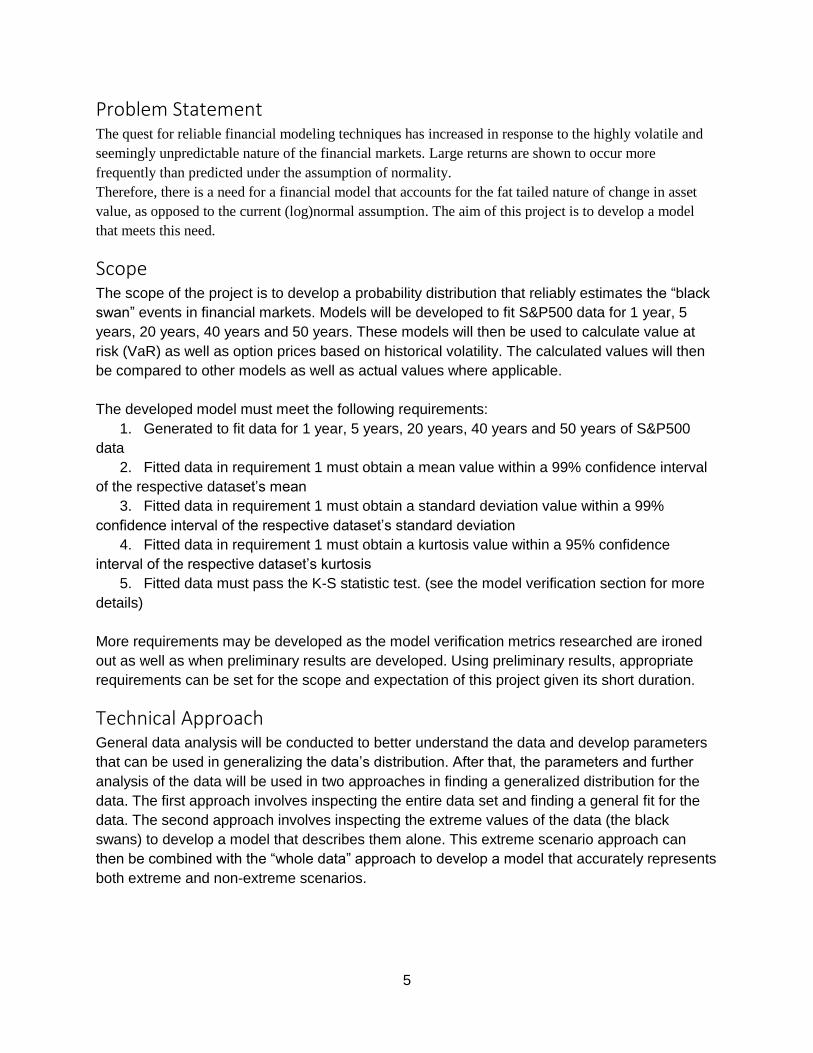
Problem Statement The quest for reliable financial modeling techniques has increased in response to the highly volatile and

seemingly unpredictable nature of the financial markets. Large returns are shown to occur more

frequently than predicted under the assumption of normality.

Therefore, there is a need for a financial model that accounts for the fat tailed nature of change in asset

value, as opposed to the current (log)normal assumption. The aim of this project is to develop a model

that meets this need.

Scope The scope of the project is to develop a probability distribution that reliably estimates the “black

swan” events in financial markets. Models will be developed to fit S&P500 data for 1 year, 5

years, 20 years, 40 years and 50 years. These models will then be used to calculate value at

risk (VaR) as well as option prices based on historical volatility. The calculated values will then

be compared to other models as well as actual values where applicable.

The developed model must meet the following requirements:

1. Generated to fit data for 1 year, 5 years, 20 years, 40 years and 50 years of S&P500

data

2. Fitted data in requirement 1 must obtain a mean value within a 99% confidence interval

of the respective dataset’s mean

3. Fitted data in requirement 1 must obtain a standard deviation value within a 99%

confidence interval of the respective dataset’s standard deviation

4. Fitted data in requirement 1 must obtain a kurtosis value within a 95% confidence

interval of the respective dataset’s kurtosis

5. Fitted data must pass the K-S statistic test. (see the model verification section for more

details)

More requirements may be developed as the model verification metrics researched are ironed

out as well as when preliminary results are developed. Using preliminary results, appropriate

requirements can be set for the scope and expectation of this project given its short duration.

Technical Approach General data analysis will be conducted to better understand the data and develop parameters

that can be used in generalizing the data’s distribution. After that, the parameters and further

analysis of the data will be used in two approaches in finding a generalized distribution for the

data. The first approach involves inspecting the entire data set and finding a general fit for the

data. The second approach involves inspecting the extreme values of the data (the black

swans) to develop a model that describes them alone. This extreme scenario approach can

then be combined with the “whole data” approach to develop a model that accurately represents

both extreme and non-extreme scenarios.

6

General Data Analysis General analysis of the dataset will be conducted to understand critical metrics of the data.

Mean, standard deviation, kurtosis and skewness values will be calculated in order to

understand the shape of the data’s distribution. These metrics can then be used in generalizing

a distribution for the data.

The data will also be checked for normality using the Anderson Darling and the Shapiro Wilk

tests to verify the assumption of fat tailed-ness.The data’s density will also be plotted so that the

distribution can be easily visualized and compared to a normal distribution. An example of this

analysis for the last 250 days of S&P 500 data is as follows:

Mean: 0.0009688516

Standard Deviation: 0.006825034

Kurtosis: 1.083292

Skewness: -0.4975298

Graph:

Whole Data Modeling

7

After obtaining the key parameters of the data, we attempt to generalize the distribution of the

data with two types of distributions. The t-distribution and a mixed normal distribution. These

distributions are commonly used to describe fat tail data sets since they can have fat tails.

t Distribution

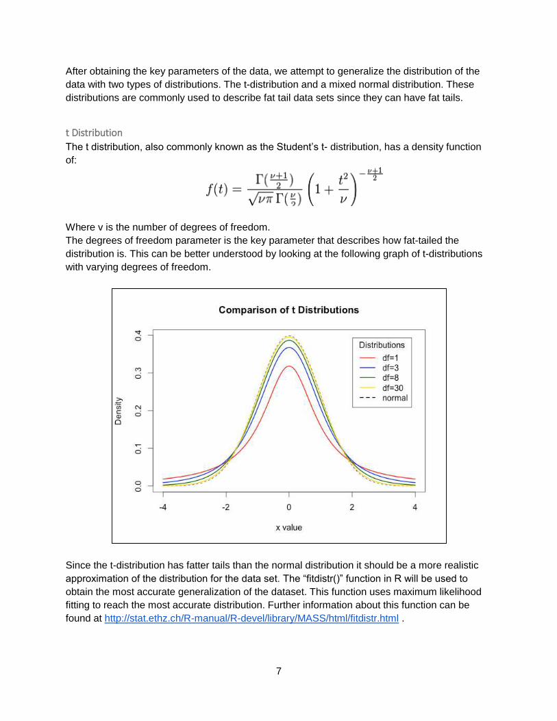
The t distribution, also commonly known as the Student’s t- distribution, has a density function

of:

Where v is the number of degrees of freedom.

The degrees of freedom parameter is the key parameter that describes how fat-tailed the

distribution is. This can be better understood by looking at the following graph of t-distributions

with varying degrees of freedom.

Since the t-distribution has fatter tails than the normal distribution it should be a more realistic

approximation of the distribution for the data set. The “fitdistr()” function in R will be used to

obtain the most accurate generalization of the dataset. This function uses maximum likelihood

fitting to reach the most accurate distribution. Further information about this function can be

found at http://stat.ethz.ch/R-manual/R-devel/library/MASS/html/fitdistr.html .

8

Mixed Normal Distribution

The second distribution used to generalize the data’s behavior will be obtained by mixing two

normal distributions of varying standard deviations. This aggregation of normal distributions with

varying standard deviations creates fatter tails than a normal distribution and can hopefully more

accurately represent the data’s distribution.

The procedure used to generate a mixed normal distribution is as follows:

1. Generate a Boolean distribution (Y) whose values are 1 with probability p and 0 with

probability 1-p

2. Generate two Gaussian random variable 𝑋1 and 𝑋2 to be mixed with standard deviations

( and 𝛽) such that the variance of the mixed model is equal to 1. This method results in only

one of the standard deviations being a parameter to the distribution while the other one is

calculated as follows

𝛽 = √1 − 𝑝𝛼2

1 − 𝑝

3. Generate a standard normal distribution Z

4. Loop through all values of the generated Boolean distribution (Y) and for each value

a. If it is equal to one, equate the output model value to α times the

value from the standard normal distribution Z,

b. otherwise equate the output model value to β times the value from

the standard normal distribution Z

In mathematical terms:

𝑌 = 𝐵𝑜𝑜𝑙(𝑝)

𝑍 = 𝑁𝑜𝑟𝑚(0,1)

𝛽 = √1 − 𝑝𝛼2

1 − 𝑝

𝐹𝑜𝑟 𝑒𝑎𝑐ℎ 𝑌

𝑖𝑓 𝑌 = 1, 𝑋 = 𝛼𝑍

𝑖𝑓 𝑌 = 0, 𝑋 = 𝛽𝑍

This generated distribution has a mean of 0, standard deviation of 1 and a kurtosis value equal

to

𝛾 = 3(𝑝𝛼4 + (1 − 𝑝)𝛽4) − 3

Graphs of mixed normal distributions with varying p, 𝛼 and kurtosis values are included in the

appendix.

In order to find a mixed normal distribution that fits the dataset accurately, MS Excel Solver is

used to obtain values for p and 𝛼 based on the kurtosis value of the data. From there, the model

is generated and plotted on a graph alongside the data for visual comparison.

9

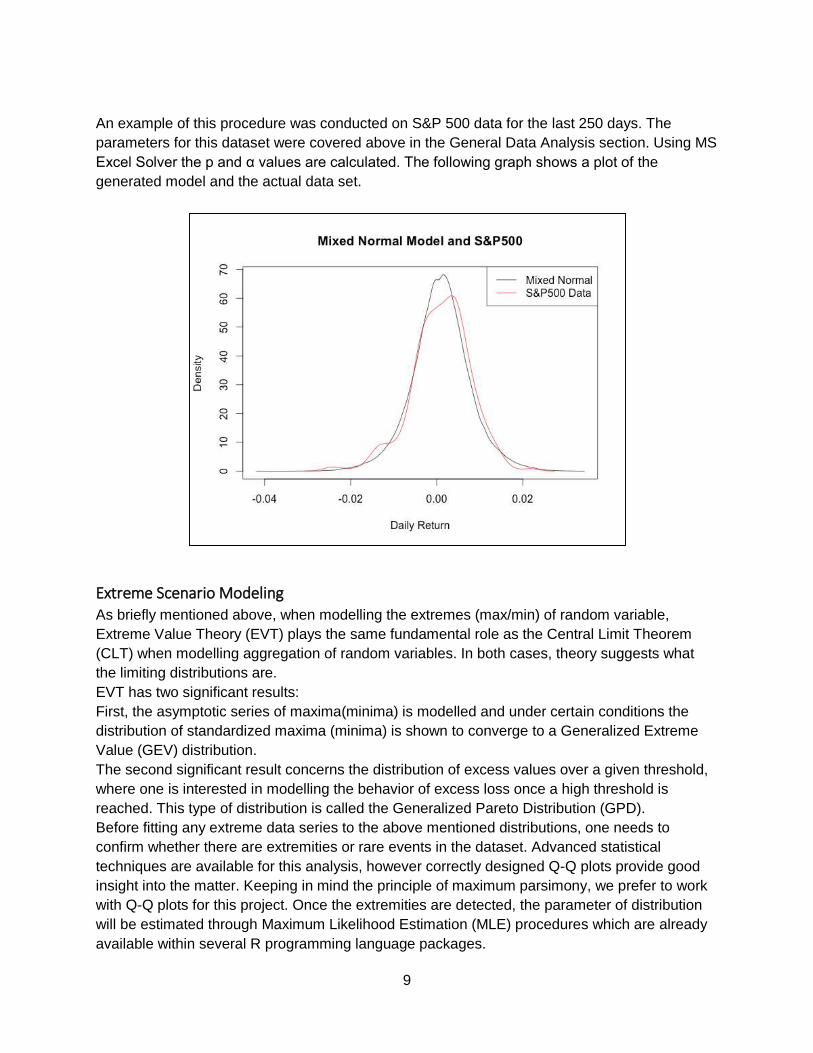
An example of this procedure was conducted on S&P 500 data for the last 250 days. The

parameters for this dataset were covered above in the General Data Analysis section. Using MS

Excel Solver the p and α values are calculated. The following graph shows a plot of the

generated model and the actual data set.

Extreme Scenario Modeling As briefly mentioned above, when modelling the extremes (max/min) of random variable,

Extreme Value Theory (EVT) plays the same fundamental role as the Central Limit Theorem

(CLT) when modelling aggregation of random variables. In both cases, theory suggests what

the limiting distributions are.

EVT has two significant results:

First, the asymptotic series of maxima(minima) is modelled and under certain conditions the

distribution of standardized maxima (minima) is shown to converge to a Generalized Extreme

Value (GEV) distribution.

The second significant result concerns the distribution of excess values over a given threshold,

where one is interested in modelling the behavior of excess loss once a high threshold is

reached. This type of distribution is called the Generalized Pareto Distribution (GPD).

Before fitting any extreme data series to the above mentioned distributions, one needs to

confirm whether there are extremities or rare events in the dataset. Advanced statistical

techniques are available for this analysis, however correctly designed Q-Q plots provide good

insight into the matter. Keeping in mind the principle of maximum parsimony, we prefer to work

with Q-Q plots for this project. Once the extremities are detected, the parameter of distribution

will be estimated through Maximum Likelihood Estimation (MLE) procedures which are already

available within several R programming language packages.

10

A problem with the EVT approach is deciding where the tail starts for any distribution’s original

data set. This problem can also be solved by visual examination of the distribution fit graphs.

Since extremities are rare by definition, we will work with large data sets of S&P 500 daily

returns.

Generalized Extreme Value (GEV) Distribution

The Generalized Extreme Value distribution can be developed as follows:

Let 𝑋𝑛 be a series of iid random variables and 𝑀𝑛 be the maxima of values of 𝑋 within certain

blocks of size 𝑚 such that 𝑀𝑛 = 𝑀𝑎𝑥 (𝑋1, 𝑋2, … 𝑋𝑛). Then 𝑀𝑛 follows the GEV distribution and

H(x):

The parameters 𝜇, 𝜎, 𝜉 correspond, respectively, to location, scale and shape (tail index)

parameters.

The basic problem before applying GEV to any dataset is defining the appropriate block size for

maxima evaluation. There is no closed form solution to this problem but there are some rules of

thumb derived from experience. For long term analysis, grouping of daily data into annual

blocks gives the best results since they cover seasonal effects. However this approach creates

problem of data availability since for 5 years, for example, there will be only 5 data points. We

are planning to define the blocks as yearly whenever applicable, otherwise we will define

smaller size blocks, e.g. weekly, monthly or quarterly. This will also allow us to test these rules

of thumb and prove their accuracy.

Although the distribution above is defined for maxima, it is easily converted to minima by

multiplying x by -1. (invariant property).

Generalized Pareto Distribution (GPD)

The Generalized Pareto Distribution can be developed as follows:

Let X be a random variable with distribution F and a threshold given xf, for U fixes < xf, Fu is the

distribution of excesses of X over the threshold U.

𝐹𝑢(𝑥) = 𝑃(𝑋 − 𝑢 <= 𝑥𝐼 𝑋 > 𝑢), 𝑥 >= 0

Once the threshold, u, is determined by an estimation procedure, the conditional distribution of

F is approximated by a GPD.

11

The parameters 𝜎, 𝜉 correspond, respectively, to scale and shape (tail index) parameters. The

interesting property of tail index parameter is that there is a relationship between this parameter

and the t distribution’s degrees of freedom.

Combined Whole Data & EVT Distribution

Since the EVT approach only provides a distribution for the extreme scenarios, a model may be

developed that combines the whole data models developed with the extreme value distributions

to obtain a model that accurately represents the dataset as a whole.

Model Verification In order to verify the developed models’ goodness of fit, several metrics will be used. Of these

metrics, the Kolmogorov-Smirnov (K-S) statistic will be used.

Other metrics are still being researched and developed in order to obtain more solid

requirements for the developed model.

Applications Two applications of the developed fat tail model will be pursued. Of the most common fields of

modeling in financial markets, risk mitigation and option pricing are extremely interesting. For

risk mitigation, the application chosen will be calculating value at risk (VaR) and for option

pricing, a Monte Carlo simulation for option pricing will be developed.

Value at Risk (VaR)

Once complete models have been developed and verified, VaR calculations will be made for

each model type and normal distribution as well for benchmarking. We will also develop some

measures of effectiveness (MoE) in order to compare each models outputs and try to identify

best approach for risk measurements. The MoE’s will be defined on principles of conservatism,

accuracy and efficiency.

Option Pricing

Once complete models have been developed and ve3rified, a Monte Carlo Simulation can be

run to simulate the expected value of an option.

The simulation will work by taking several inputs (Strike price, duration, risk free rate, discount

rate, and replication count) in addition to model information (volatility, distribution). It will then

generate daily values for change in price based on the model. Once the duration given to the

simulation has run, it can calculate an expected value for option prices than can be compared to

actual prices of options, as well as Black-Scholes prices using historical volatility, to verify the

model.

Expected Results

12

The results of this project are twofold, to reach a model that can accurately depict a data set of

a fat tailed distribution and to be able to apply the developed model in financial applications to

achieve more realistic values and be capable of making more informed decisions.

Expected Model Results

In general, the expected results for the modeling portion of the project are to find at least 1

model that can accurately depict the dataset’s distribution. The expected model results are

described for each of the attempted modeling techniques as follows:

t-Distribution

The t-distribution model should be an effective method in accurately generalizing a distribution

for the data obtained for S&P500. This distribution has been used by several research parties in

depicting a fat tail distribution. The t-distribution is expected to be the best generalized model for

a an entire data set as opposed to splitting up the dataset into extreme and non-extreme values.

Mixed Normal Distribution

Based on preliminary results of the mixed normal distribution shown above, it seems that the

approach used to achieve an accurate model is valid. Further inspection with quality metrics

needs to occur in order to accurately know how well the model is at fitting the data. With

applying this model, we can also find out how well it is compared to the t distribution.

GEV and GPD Distributions

We expect to estimate the parameters of those distributions for S&P 500 Index data for different

time frames within some confidence levels. If we have enough time, we are planning to conduct

sensitivity analysis of those point estimations on developed models.

Expected Application Results For VaR calculations, we expect different estimates for each type of modelling approaches.

After we compare those estimates with respect to MoE’s that we will develop, hopefully we will

select best model for S&P 500 index. We also plan to compare each modelling approach with a

range of confidence levels of VaR calculations. In theory, EVT modelling approach performs

better at high confidence levels, i.e. %99 or more.

For options pricing, we plan to compare option price estimates of each modelling approach

including normal distribution with historical market prices for set options with given maturity and

strike price. In order to make meaningful comparisons of option prices, we will use series of

price estimates and apply statistical tests. Hopefully, we expect to define better estimation

methodology than current Black Scholes model, which depends upon normality assumption.

13

Project Plan This project aims to follow the following work breakdown structure and schedule:

Project

1.0 Definition

1.1 Context

1.2 Problem

1.3Scope

2.0 Model

2.1 Data Analysis2.2 Whole Data

Model

2.2.1 Mixed Normal Model

2.2.2 t Distribution

Model

2.3 Extreme Scenario Model

2.3.1 GEV Model

2.3.2 GPD Model

2.3.3 Combined Model

3.0 Model Applications

3.1 VaR Calculations

3.2 Option Pricing

4.0 Deliverables

4.1 Problem Presentation

4.2 Scope Presentation

4.3 Proposal

4.4 Progress Reports

4.5 Dry Runs

4.6 Website

4.7 Report

4.8 Final Presentation

14

The following is the Gantt Chart for the schedule. The critical path is highlighted in red.

15

16

17

References

Value At Risk: A Quantile-Based Distribution Approach For Incorporating Skewness And Fat-

Tailedness, Doowoo Nam

Alternative statistical distributions for estimating value-at-risk: theory and evidence, Cheng-Few

Lee and Jung-Bin Su

Implementable tail risk management: An empirical analysis of CVaR-optimized carry trade

portfolios, Hakan Kaya, Wai Lee, Bobby Pornrojnangkool

An Empirical Examination of Extreme Value Theory Methods in VaR Estimation, Zhenhong Faa

Capturing fat tails, Zari Rachev,Boryana Racheva-Iotova and Stoyan Stoyanov

Estimating Flexible, Fat-Tailed Asset Return Distributions, Craig Friedman, Yangyong Zhang,

and Jinggang Huang

Estimation of portfolio return and value at risk using a class of gaussian mixture distributions,

Kangrong Tan, Meifen Chu

A Comparative Software Review for Extreme Value Analysis, Eric Cilleland, Mathieu Ribatet,

Alec G Stephenson

VaR-x: Fat tails in financial risk management, Ronals Huisman, Kees G Koedijk and Rachel A J

Pownall

Fat-tailed models for risk estimation, Stoyan V. Stoyanov, Svetlozar T. Rachev, Boryana

Racheva-Iotova, Frank J. Fabozzi

Fat tails via utility based entropy, Craig Freedman, Yangyong Zhang, Wenba Cao

An Application of Extreme Value Theory for Measuring Financial Risk, Manfred Gilli and Evis

KÄellezi

Option Pricing and Implied Tail Indices under the Generalised Extreme Value (GEV)

Distribution, Amadeo Alentorn

Intrinsic bubbles and fat tails in stock prices: a note, Prasad V. Bidarkota and Brice V. Dupoyet

Risk Forecasting with GARCH, Skewed t Distributions, and Multiple Timescales, Alec N.

Kercheval and Yang Liu

Portfolio optimization with serially correlated, skewed and fat tailed index returns, M.

Glawischnig and I. Seidl

18

Return Distributions and Applications, Young Do Kim

Computational aspects of risk estimation in volatile markets: A survey, Stoyan V. Stoyanov,

Svetlozar T. Rachev, Frank J. Fabozzi

Backtesting Value-at-Risk based on Tail Losses, Woon K. Wong

Statistical modeling of finance data and extensions of option pricing framework, Xin Zhong

Steps in Applying Extreme Value Theory to Finance: A Review, Younes Bensalah

The Tail Fatness and Value-at-Risk Analysis of TAIFEX and SGX-DT Taiwan

Stock Index Futures, Yu Chuan Huang, Chu-Hsiung Lin, Chang-Cheng Chang Chien and Bor-

Jing Lin

The tale of the tail: extreme-value patterns of financial returns, Angelo Corelli

19

Appendix The following are graphs of generated data of mixed normal distributions.