applications of doe in engineering and science: a
TRANSCRIPT
__________________________________________________________
Applications of DOE in Engineering and Science: A Collection of 26 Case Studies
Leonard M. Lye
PhD, PEng, FCSCE, FEC, FEIC, FCAE
Professor Emeritus Faculty of Engineering and Applied Science
Memorial University of Newfoundland
1st Edition (Revised)
Copyright © 2019 by Leonard M Lye, St. John’s, Newfoundland, Canada
__________________________________________________________

i
Forward to Use of DOE in Engineering and Science
Dr. Lye’s association with Stat-Ease and me goes back to 2005 when he started using our software for teaching DOE. He came to our headquarters in Minneapolis for a workshop and gave us a book on Newfoundland that inspired me to visit him in St. John’s in 2018. Dr. Lye told me then that upon his retirement from Memorial University he would devote time to a comprehensive collection of DOE case studies. I am very pleased to see this come to fruition.
I did my first DOE in 1974 and took to this multifactor testing approach immediately as a catalyst for my work as a chemical engineer working on process development. Why anyone would continue to study only one factor at a time (OFAT) remains a mystery to me. However, OFAT being established throughout the educational process as the scientific method cannot be easily undone in the minds of highly-trained experimenters. The only way that I’ve found to do so is by presenting relevant examples. This book by Dr. Lye provides a treasure trove for anyone who wants to persuade others to do DOE or those that seek compelling evidence of its advantages for their research work.
Now that Dr. Lye has done such a great service to the field of DOE by presenting these 64 examples, I hope that he will turn his attention to making his DOE-GolferTM training device legal for use on the course. That will solve all my problems for putting. However, I will settle for Dr. Lye sparing time from happy retirement to continue his good work spreading the good word about DOE. Well done!
- Mark J. Anderson, PE, CQE Principal, Stat-Ease, Inc. Minneapolis, MN, USA
July 9, 2019


1
______________________________________________ PREFACE
“The only way to know how a complex system will behave — after you modify it — is to modify it and see how it behaves.” George Box
Since 1995, I have been teaching a graduate course strangely titled “Similitude, Modelling, and Data Analysis” ENGI 9516 at the Faculty of Engineering and Applied Science, Memorial University of Newfoundland. The original instructor of this course, Dr. James Sharp, was an expert in the field of hydraulics with particular expertise in hydraulic models and dimensional analysis. He taught this course for many years and also wrote several books on these subjects. A few years before he retired, he asked me to co-teach the course. Since my expertise is in statistical hydrology, I added a few topics on data analysis, particularly regression analysis. When Dr. Sharp retired, I became the sole instructor of the course, and as I am not an expert in similitude or dimensional analysis, the current course content is mostly on the design and analysis of multifactor experiments. Dimensional analysis and how it can be combined with modern design of experiment methodologies is now only a small part of my course. However, to prevent unnecessary university calendar changes, the name of the course has remained the same. The course is now better known as the Design of Experiment or the DOE course and is one of the core courses for graduate students in engineering. Students taking the course come from all disciplines of engineering and from the Faculty of Science. Over the years, the class size has grown from about 20 students to 40-50, in recent years. The course covers the following topics:
1. Design of Experiments, definition of and strategies for experimentation 2. Factorial vs. one-factor-at-a-time (OFAT) experiments 3. Review of one-factor experiments, regression, and ANOVA 4. General factorial experiments 5. Design and analysis of 2-level factorial experiments 6. Concepts of blocking and confounding 7. Fractional factorial design and analysis, fold-over designs 8. Response Surface Methodology (RSM): Central Composite Design (CCD), and Box-
Behnken Design (BBD) 9. Design for computer experiments, uniform designs, and other designs 10. Restricted randomization and hard-to-change factors 11. Optimal designs, multiple linear constraints, and definitive screening designs. 12. Methods of dimensional analysis 13. The combined use of DOE and dimensional analysis Mixture designs, combined mixture-process designs, Taguchi methods, and other advanced topics are not covered.
The use of design of experiments (DOE) methodologies such as the topics covered in the course has increased exponentially over the years in almost all areas of science and engineering. There

2
are also many textbooks by both statisticians and others that cover topics related to the statistical design of experiments.
Over the last 20 or more years, I have learned that, according to my students, one of the most useful parts of the course is reviewing journal papers that use DOE methods in experiments. Students are asked to search for journal papers in their discipline or field of interest and do a thorough review. This review requires that students identify the objectives of the paper, the factors used in the experiment, the responses measured, and the choice of experimental design. Then students must evaluate the correctness of the statistical analyses, and the results. Invariably, on reanalysis of the data given in the paper, the students often find that the data reported may be wrong, the statistical model choice is wrong, or the ANOVA assumptions may not have been checked. Or, the students may find the results reported are not reproducible. Having students review published journal papers provides an opportunity to develop confidence in their knowledge of DOE and helps students realize that not all published papers can be taken at face value. Important errors in analysis or data can be missed either by the authors or reviewers despite the fact that many of the reviewed papers are published in reputable journals.
Over the years, I have amassed a large collection of journal and some conference papers that use DOE methodologies in engineering and science. This book provides a selection of 26 case studies from this collection. The case studies cover a wide range of applications in engineering and science. I chose only papers where there is a complete set of data available for reanalysis. The selection is not exhaustive and does not cover every discipline of engineering or science. However, I hope that readers of the book get a good sense of the wide application of DOE methods, and will try their hand at analyzing the published data. The methods most commonly used in the papers deal mainly with factorial designs, fractional factorial designs, and response surface methodologies, particularly the use of the central composite and Box-Behnken designs.
The book is ideal for students who have taken or is taking a course in DOE. It is also useful for those who want to learn more about the power of DOE methods or who are looking for research ideas. Each dataset is available in print form in the book and available as an Excel file (.xls) and as a Design-Expert® file (.dxpx). Hence this collection of case studies is also be a good resource for instructors of DOE. Please contact me at [email protected] for the files.
I want to thank the hundreds of students who have taken my course over the years and the feedback they have offered. I learned so much from interacting with them and helping them design unique experiments for their thesis and other research work. I would particularly like to acknowledge the unwavering support of Mark Anderson of Stat-Ease Inc. the publisher of Design-Expert® software, by providing a free 6-month version of their software to my students each year. My class has been using Design-Expert® as the software of choice since version 5. There are other statistical packages available for DOE such as Excel Add-ins, Minitab, and JMP, but I have found Design-Expert® to be comprehensive and easy to use. Furthermore, the company Stat-Ease Inc. provides excellent support through their website, YouTube channel, and regular webinars.
Leonard Lye St. John’s, Newfoundland, Canada
3
______________________________________________
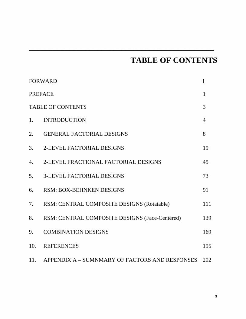
TABLE OF CONTENTS
FORWARD i
PREFACE 1
TABLE OF CONTENTS 3
1. INTRODUCTION 4
2. GENERAL FACTORIAL DESIGNS 8
3. 2-LEVEL FACTORIAL DESIGNS 19
4. 2-LEVEL FRACTIONAL FACTORIAL DESIGNS 45
5. 3-LEVEL FACTORIAL DESIGNS 73
6. RSM: BOX-BEHNKEN DESIGNS 91
7. RSM: CENTRAL COMPOSITE DESIGNS (Rotatable) 111
8. RSM: CENTRAL COMPOSITE DESIGNS (Face-Centered) 139
9. COMBINATION DESIGNS 169
10. REFERENCES 195
11. APPENDIX A – SUMNMARY OF FACTORS AND RESPONSES 202

4
______________________________________________ 1. INTRODUCTION
This book provides a collection of 26 case studies in the field of engineering and science based on articles published in a wide variety of journals from 2000 to 2018. The methodology used in each study falls into one of eight types which form the eight main chapters of this book. These methods are:
• General factorial designs • 2-level factorial designs or 2k designs • 2-level fractional factorial designs or 2k-p designs • 3-level factorial designs or 3k designs • Response surface methodology or RSM: Box-Behnken designs or BBD • Response surface methodology or RSM: Rotatable Central composite design or CCD • Response surface methodology or RSM: Face Centered Central composite design or FCD • Combination designs
The chapter on general factorial designs has four case studies on the use of multi-factored general factorial design with a different number of levels for each factor. There are 10 case studies on the use of 2-level factorial designs, nine on 2-level fractional factorial designs, and six on 3-level factorial designs. There are three chapters on the use of response surface methodology or RSM sub-divided as follows: Box-Behnken design or BBD (eight case studies), rotatable Central Composite Designs or CCD (10 case studies), and face-centered designs or FCD (10 case studies). Rotatable and face-centered designs are in two separate chapters. Combination designs are those that use more than one type of design. They could be a 2-level factorial or a 2-level fractional factorial design, followed by a RSM design. There are seven case studies of this type. The number of case studies in each chapter roughly represents the popularity of each design.
The field of experimental design is very wide and this book only covers the most common DOE methodologies found in journals of science and engineering. Other DOE methodologies such as Latin square designs, repeated measures design, nested designs, optimal designs, space-filling designs, definitive screening designs, split-plot designs, mixture designs, and other less commonly used or more advanced methodologies are not covered.
The case studies in this book are based on articles published in over 55 different journals and shows the wide application of DOE methodology in science and engineering. As mentioned in the Preface, only papers that contain the complete design and responses are included so that readers can analyse the data for themselves and compare their results with those presented in the paper. Naturally the list of journals is not exhaustive. In alphabetical order, the list of journals is as follows. Case study and page numbers are shown for ease of reference.
Advances in Environmental Research – CS #2.1, p 8.
Applied Mathematical Modelling – CS #3.7, p 37.

5
Applied Stochastic Models in Business and Industry – CS #8.1, p 139.
Applied Thermal Engineering – CS #6.3, p 96.
ASCE Journal of Environmental Engineering – CS #6.8, p 107.
Bioresource Technology – CS #8.5, p 150; CS #9.1, p 169; CS #9.6, p 187; CS #9.7, p 189.
Biotechnology Progress – CS #4.2, p 48.
Carbohydrate Polymers – CS #6.7, p 106.
Cement and Concrete Composites – CS #6.6, p 102.
Colloids and Surfaces A: Physicochemical Engineering Aspects – CS #7.9, p 133.
Computers and Chemical Engineering – CS #8.7, p 156.
Construction and Building Materials – CS #6.2, p 93.
Desalination – CS #5.6, p 86.
Desalination and Water Treatment – CS #3.2, p 22; CS #5.5, p 84.
Environmental Science and Technology – CS #7.1, p 111.
Food Chemistry – CS #7.6, p 125.
Fuel – CS #6.1, p 91.
Fuel Processing Technology – CS #8.4, p 148.
IEEE Transactions on Magnetics – CS #8.4, p 148.
Industrial Crops and Products – CS #4.9, p 70.
International Communications in Heat and Mass Transfer – CS #8.2, p 142.
International Journal of Food Science and Technology – CS #4.3, p 52.
International Journal of Hydrogen Energy – CS #7.5, p 123.
International Journal of Mining Science and Technology – CS #3.4, p 29.
Journal on Applied Signal Processing – CS #4.7, p 65.
Journal of ASTM International – CS #7.8, p 131.
Journal of Biomedicine and Biotechnology – CS #9.3, p 177.
Journal of Chemical Technology and Biotechnology – CS #9.2, p 173.
Journal of Engineering – CS #3.9, p 41.
Journal of Food Engineering – CS #7.3, p 118; CS # 8.8, p 160.
Journal of Hazardous Materials – CS #7.2, p 115; CS #7.7, p 128.
Journal of King Saud University-Engineering Sciences – CS #5.2, p 75.
6
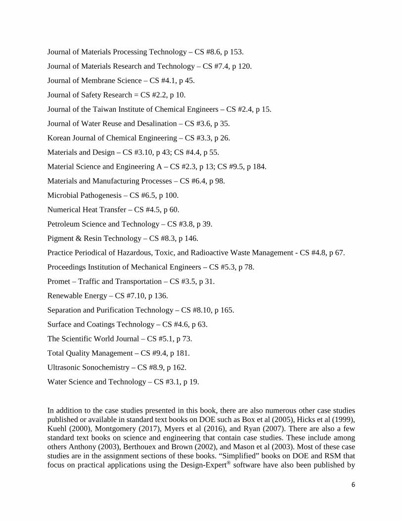
Journal of Materials Processing Technology – CS #8.6, p 153.
Journal of Materials Research and Technology – CS #7.4, p 120.
Journal of Membrane Science – CS #4.1, p 45.
Journal of Safety Research = CS #2.2, p 10.
Journal of the Taiwan Institute of Chemical Engineers – CS #2.4, p 15.
Journal of Water Reuse and Desalination – CS #3.6, p 35.
Korean Journal of Chemical Engineering – CS #3.3, p 26.
Materials and Design – CS #3.10, p 43; CS #4.4, p 55.
Material Science and Engineering A – CS #2.3, p 13; CS #9.5, p 184.
Materials and Manufacturing Processes – CS #6.4, p 98.
Microbial Pathogenesis – CS #6.5, p 100.
Numerical Heat Transfer – CS #4.5, p 60.
Petroleum Science and Technology – CS #3.8, p 39.
Pigment & Resin Technology – CS #8.3, p 146.
Practice Periodical of Hazardous, Toxic, and Radioactive Waste Management - CS #4.8, p 67.
Proceedings Institution of Mechanical Engineers – CS #5.3, p 78.
Promet – Traffic and Transportation – CS #3.5, p 31.
Renewable Energy – CS #7.10, p 136.
Separation and Purification Technology – CS #8.10, p 165.
Surface and Coatings Technology – CS #4.6, p 63.
The Scientific World Journal – CS #5.1, p 73.
Total Quality Management – CS #9.4, p 181.
Ultrasonic Sonochemistry – CS #8.9, p 162.
Water Science and Technology – CS #3.1, p 19.
In addition to the case studies presented in this book, there are also numerous other case studies published or available in standard text books on DOE such as Box et al (2005), Hicks et al (1999), Kuehl (2000), Montgomery (2017), Myers et al (2016), and Ryan (2007). There are also a few standard text books on science and engineering that contain case studies. These include among others Anthony (2003), Berthouex and Brown (2002), and Mason et al (2003). Most of these case studies are in the assignment sections of these books. “Simplified” books on DOE and RSM that focus on practical applications using the Design-Expert® software have also been published by

7
Anderson and Whitcomb (2015, 2016) who are principals at Stat-Ease Inc., publisher of the software. Other software for DOE and RSM besides Design-Expert include JMP by SAS, Minitab® by Minitab Inc., Fusion-Pro by S-Matrix, among many others.
The case studies in each chapter of this book are arranged by alphabetical order of the first author’s last name. Each case study describes the objective of the experiment, the number of factors and responses in the experiment, the type of design used, the full data set resulting from the experiment, the software used, and a summary of the results obtained by the authors. I encourage the reader to read the original papers and re-analyze the data to compare with the results obtained by the authors. If you find that you obtain the same results, then congratulate yourself and the authors for correctly doing the analysis. If you did not get the same results, here is your opportunity to figure out why. Were the assumptions of regression checked? Were the correct model terms included in the final model? Were you able to obtain a better model? Should there be a transformation for the response? Sometimes there are differences because of the software used, and sometimes there could be typographical errors. In any case, reanalyzing published data is a great learning experience.
Disclaimer
While every effort has been made to reproduce the data and tables in the published papers as accurately as possible, it is advisable that the reader read the original papers for the details of the experiments carried out and to ensure that the data and tables presented here are indeed correct.

8
______________________________________________ 2. GENERAL FACTORIAL DESIGNS
Four case studies using general factorial designs are presented in this Chapter. The number of factors ranges from three to four. For each case study, the factors have a differing number of levels ranging from two to five levels.
Case Study #2.1
Annadurai, G., Ruey-Shin Juang, and Duu-Jong Lee (2002): Factorial design analysis for adsorption of dye on activated carbon beads incorporated with calcium alginate. Advances in Environmental Research, 6, pp. 191-198.
This study used a factorial design with three factors to investigate the batch adsorption equilibrium of the dye Rhodomine 6G, using activated carbon beads incorporated with calcium alginate (ACCA beads). The effect of three factors that govern the adsorption process, dye concentration in mg/l, pH, and temperature °C were considered. The factors and levels are shown in Table 2.1.
Table 2.1: Factors and levels for adsorption of dye study.
Factor Description Unit Level 1 Level 2 Level 3 A Init. Dye Concentration Mg/l 100 200 300 B pH 7 8 9 C Temperature °C 30 60
The response was the percentage of adsorption of Rhodamine 6G using a fixed dosage of ACCA beads (1 g/l).
Three levels of dye concentrations (100, 200, 300) and pH (7, 8, 9) were used and the temperature was at two levels (30 °C and 60 °C). In total there were (3 x 3 x 2 = 18) runs. The run combinations and responses are shown in Table 2.2. These were taken from Tables 2 and 3 of Annadurai et al (2002).
According the authors, the use of the factorial design and subsequent ANOVA allowed a polynomial model to be fitted, shown in Equation (1) of the paper. The method used to calculate the effects and their sum of squares are given in the paper. There is no mention if any software was used for the ANOVA calculations.

9
Table 2.2: Operating conditions and responses (after Annadurai et al, 2002).
Trial No.
Dye Concentration
(mg/l) pH Temperature
(°C) % dye
adsorption Predicted value (%)
1 100 7 30 98.50 98.47 2 200 7 30 96.70 96.77 3 300 7 30 94.80 95.07 4 100 8 30 98.70 98.71 5 200 8 30 97.00 97.01 6 300 8 30 95.30 95.31 7 100 9 30 99.20 98.95 8 200 9 30 97.30 97.25 9 300 9 30 95.60 95.55
10 100 7 60 99.90 99.80 11 200 7 60 98.20 98.10 12 300 7 60 96.40 96.40 13 100 8 60 100.00 100.04 14 200 8 60 98.60 98.34 15 300 8 60 96.70 96.64 16 100 9 60 100.00 100.02 17 200 9 60 98.20 98.59 18 300 9 60 97.10 96.89
The ANOVA results were shown in Table 5 of the paper and are reproduced here as Table 2.3. The R2 was given as 0.9884 based on fitting a linear model. The model was not shown in the paper but the authors gave the predicted values together with the actual values of the responses in Table 4 of their paper. These predicted values are shown here in Table 2.2. Table 2.3: Regression analysis for adsorption of dye by linear model fitting (ANOVA). Table 5 of Annadurai et al (2002).
Source Sum of Squares df
Mean Square F-value P-value
Model 43.38 3 14.46 396.73 <0.0001 Residual 0.51 14 0.036 Corr. Total 43.89 17
R2 = 0.9884
From Table 2.3, no interaction or quadratic terms were included in the model. It is not mentioned whether the assumptions of regression were checked. The authors concluded that the initial dye concentration has the most significant effect while the temperature has the least effect on the percentage of dye adsorption.

10
Case Study #2.2
Al-Darrab, I. A., Zahid A. Khan, and Shiekh I. Ishrat (2009): An experimental study on the effect of mobile phone conversation on drivers’ reaction time in braking response. Journal of Safety Research, 40, pp. 185-189.
This study considered the effect of three factors on drivers’ reaction time in braking. The aim of the study was primarily to investigate the effect of mobile phone use on driving performance. The factors and levels are shown in Table 2.4:
Table 2.4: Factors and levels for mobile phone study.
Factor Description Unit Level 1 Level 2 Level 3 A Distance between cars m 10 15 20 B Call Duration s 30 60 90 C Time of driving Day Night
Response = RT, Drivers’ reaction time (s)
This experiment had three levels for Factor A and B, and two levels for Factor C. The number of replications was three. The total number of runs was 3 x (3 x 3 x 2) = 54. Two cars travelling at a given distance apart (Factor A) were used. Factor B, the call duration, refers to the time spent talking on a mobile phone. For Factor C, day time is from 1600 to 1800 hours, and night time is from 2030 to 2230 hours. Twenty seven (27) volunteer drivers were used in the experiment where each driver was randomly assigned to two run combinations. The location of the study was in Jeddah, Saudi Arabia. The detailed experimental procedure was explained in the paper.
Design Expert by Statease Inc. was used for the design and analysis. The version of the software was not mentioned.
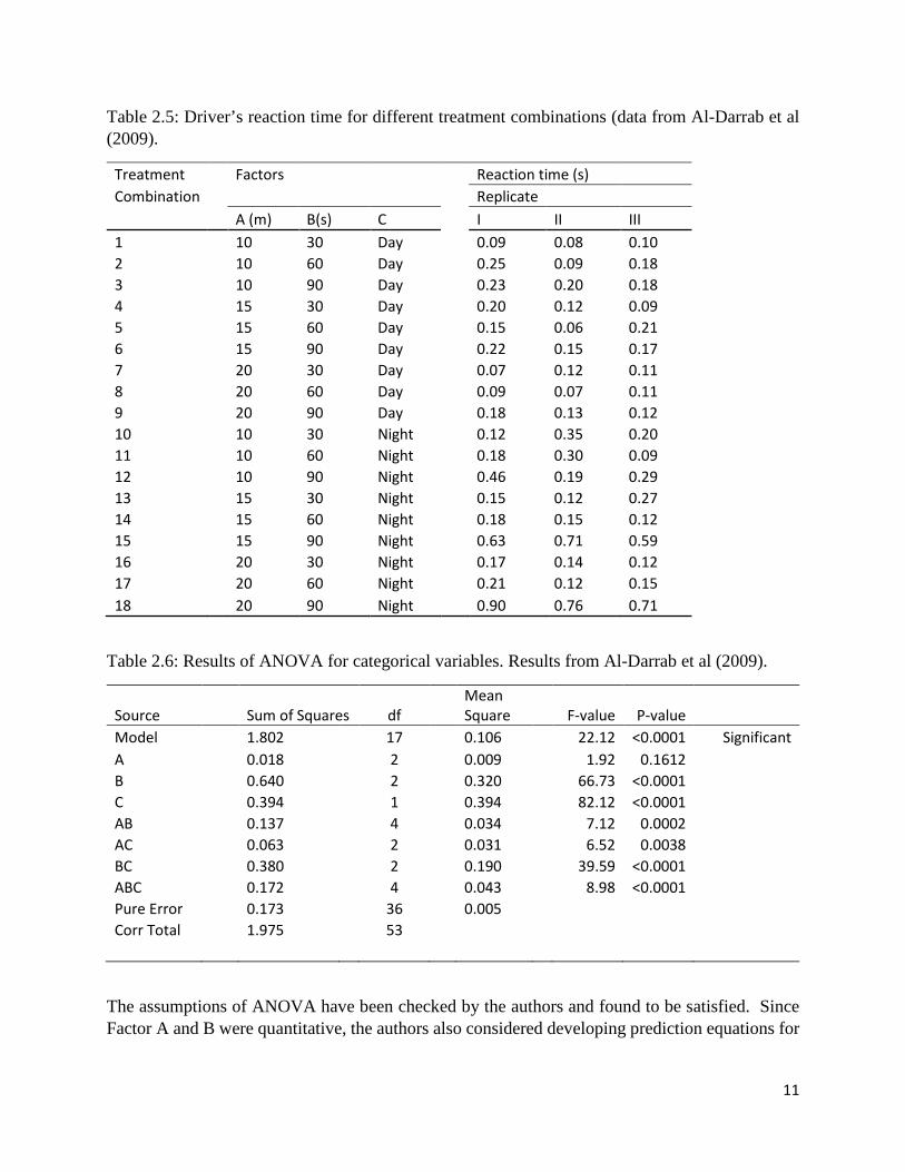
The results of the experiment were given in Table 2 of the paper, and are reproduced here in Table 2.5.
For the initial analysis, the authors treated each factor as categorical. The ANOVA results are shown in Table 2.6.
11
Table 2.5: Driver’s reaction time for different treatment combinations (data from Al-Darrab et al (2009).
Treatment Factors Reaction time (s) Combination Replicate A (m) B(s) C I II III 1 10 30 Day 0.09 0.08 0.10 2 10 60 Day 0.25 0.09 0.18 3 10 90 Day 0.23 0.20 0.18 4 15 30 Day 0.20 0.12 0.09 5 15 60 Day 0.15 0.06 0.21 6 15 90 Day 0.22 0.15 0.17 7 20 30 Day 0.07 0.12 0.11 8 20 60 Day 0.09 0.07 0.11 9 20 90 Day 0.18 0.13 0.12 10 10 30 Night 0.12 0.35 0.20 11 10 60 Night 0.18 0.30 0.09 12 10 90 Night 0.46 0.19 0.29 13 15 30 Night 0.15 0.12 0.27 14 15 60 Night 0.18 0.15 0.12 15 15 90 Night 0.63 0.71 0.59 16 20 30 Night 0.17 0.14 0.12 17 20 60 Night 0.21 0.12 0.15 18 20 90 Night 0.90 0.76 0.71
Table 2.6: Results of ANOVA for categorical variables. Results from Al-Darrab et al (2009).
Source Sum of Squares df Mean Square F-value P-value
Model 1.802 17 0.106 22.12 <0.0001 Significant A 0.018 2 0.009 1.92 0.1612 B 0.640 2 0.320 66.73 <0.0001 C 0.394 1 0.394 82.12 <0.0001 AB 0.137 4 0.034 7.12 0.0002 AC 0.063 2 0.031 6.52 0.0038 BC 0.380 2 0.190 39.59 <0.0001 ABC 0.172 4 0.043 8.98 <0.0001 Pure Error 0.173 36 0.005 Corr Total 1.975 53
The assumptions of ANOVA have been checked by the authors and found to be satisfied. Since Factor A and B were quantitative, the authors also considered developing prediction equations for
12
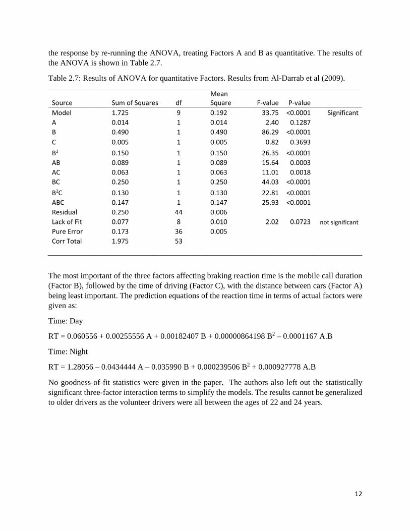
the response by re-running the ANOVA, treating Factors A and B as quantitative. The results of the ANOVA is shown in Table 2.7.
Table 2.7: Results of ANOVA for quantitative Factors. Results from Al-Darrab et al (2009).
Source Sum of Squares df Mean Square F-value P-value
Model 1.725 9 0.192 33.75 <0.0001 Significant A 0.014 1 0.014 2.40 0.1287 B 0.490 1 0.490 86.29 <0.0001 C 0.005 1 0.005 0.82 0.3693 B2 0.150 1 0.150 26.35 <0.0001 AB 0.089 1 0.089 15.64 0.0003 AC 0.063 1 0.063 11.01 0.0018 BC 0.250 1 0.250 44.03 <0.0001 B2C 0.130 1 0.130 22.81 <0.0001 ABC 0.147 1 0.147 25.93 <0.0001 Residual 0.250 44 0.006 Lack of Fit 0.077 8 0.010 2.02 0.0723 not significant Pure Error 0.173 36 0.005 Corr Total 1.975 53
The most important of the three factors affecting braking reaction time is the mobile call duration (Factor B), followed by the time of driving (Factor C), with the distance between cars (Factor A) being least important. The prediction equations of the reaction time in terms of actual factors were given as:
Time: Day
RT = 0.060556 + 0.00255556 A + 0.00182407 B + 0.00000864198 B2 – 0.0001167 A.B
Time: Night
RT = 1.28056 – 0.0434444 A – 0.035990 B + 0.000239506 B2 + 0.000927778 A.B
No goodness-of-fit statistics were given in the paper. The authors also left out the statistically significant three-factor interaction terms to simplify the models. The results cannot be generalized to older drivers as the volunteer drivers were all between the ages of 22 and 24 years.

13
Case Study #2.3
Grosselle, F., Giulio Timelli, and Franco Bonollo (2010): DOE applied to microstructural properties of Al-Si-Cu-Mg casting alloys for automotive applications. Material Science and Engineering A, 527, pp. 3536-3545.
The basic aim of the study was to investigate the solidification rate and the effect of T7 heat treatment on microstructural and mechanical properties of cast AlSi7CuMg based alloy for engine block application. That is, by studying the effect of each factor and their interactions on the production of the alloy, the authors were trying to determine whether there is potential to improve performance of the alloy. The four factors were the cooling rate measured by the secondary dendrite arm spacing (SDAS), Titanium content (Ti) Copper content (Cu), and T7 heat treatment. The process factors with their different levels are shown in Table 2.8.
Table 2.8: Process factors with their levels of observation. From Grosselle et al (2010).
Factor designation
Factor name Lower level Central level Higher level
A SDAS (µm) 17 - 34 B Titanium content (wt.%) 0 - 0.2 C Copper content (wt.%) 2 3 4 D T7 heat treatment 0 (no) 1 (yes)
Five different responses were measured. These were: equivalent diameter (d) and roundness (r) of the eutectic Si particles, yield strength (YS), ultimate tensile strength (UTS), and elongation to fracture (sf).
The first two responses were obtained from microstructural analysis using an optical microscope and quantitatively analyzed with an image analyzer. The next three responses concerned the effects of the factors on strength related properties. These were obtained from a computer controlled tensile testing machine. The details on how the images were analyzed and how the tensile tests were carried out were described in the paper.
This experiment had 2 levels for Factor A, B, and D, and 3 levels for Factor C. The total number of run combinations was (2 x 2 x 3 x 2) = 24. These run combinations were labelled P1 to P24 by the authors. Hence, a general factorial design was used.
Table 2.9 shows the run combinations together with the five responses obtained from the experiments. In the paper, for each response, the corresponding standard deviation was also given. However, these standard deviations are not shown in Table 2.9 because they were not analyzed by the authors. The run combinations were given in Table 2, and the responses were given in Tables 4 and 5 of the paper.
The software used for the design and analysis of the experiment was not mentioned. However, from the printout of the results, my guess is that the authors used Minitab.

14
Table 2.9: Run combinations and responses. Tables 2, 4 and 5 of Grosselle et al (2010).
Run SDAS (µm) Ti (%) Cu (%)
Heat treat
d (µm) r
YS (MPa)
UTS (MPa) Sf (%)
P01 17 0 2 0 2.3 4.1 159 210 1.3 P02 34 0 2 0 4.6 5.4 161 204 1.1 P03 17 0.2 2 0 2.9 4.3 137 209 1.7 P04 34 0.2 2 0 4.8 4.7 161 214 1.3 P05 17 0 3 0 3.3 5.1 160 212 1.1 P06 34 0 3 0 4.5 5.2 172 210 0.0 P07 17 0.2 3 0 4.4 6.6 171 213 0.5 P08 34 0.2 3 0 6.3 6.3 182 225 1.1 P09 17 0 4 0 2.7 3.9 169 242 1.4 P10 34 0 4 0 4.5 5.4 182 218 0.9 P11 17 0.2 4 0 4.3 3.9 187 227 0.9 P12 34 0.2 4 0 7.5 7.1 187 207 0.7 P13 17 0 2 1 2.9 1.7 255 292 1.4 P14 34 0 2 1 4.2 2.9 244 272 1.1 P15 17 0.2 2 1 3.5 2.3 261 308 1.7 P16 34 0.2 2 1 5.3 3.5 258 278 0.9 P17 17 0 3 1 2.8 2.0 268 305 1.2 P18 34 0 3 1 4.1 2.5 266 289 1.0 P19 17 0.2 3 1 4.2 2.5 260 309 1.6 P20 34 0.2 3 1 5.4 2.5 263 296 1.1 P21 17 0 4 1 2.6 1.7 256 316 1.7 P22 34 0 4 1 3.7 2.5 256 284 1.0 P23 17 0.2 4 1 4.0 2.5 279 321 1.2 P24 34 0.2 4 1 5.7 2.6 267 289 0.9
No ANOVA tables were reported in the paper. However, the main effects and some interaction plots and Pareto charts were given for each response. The prediction equations using only statistically significant terms at α=0.05, for each response, and the corresponding R2 are given below.
(i) Equivalent diameter of eutectic Si particles, d.
d = 0.93 + 0.12 SDAS – 8.28 Ti – 0.073 Cu + 4.62 Ti.Cu R2 = 0.82
(ii) Roundness of eutectic Si particles, r.
r = 1.64 + 0.07 SDAS + 3.99 Ti – 1.17 T7 R2 = 0.87
The variable T7 is either 0 for as-cast, or 1 for T7 heat treated conditions.

15
(iii) Yield strength, YS.
YS = 186.2 + 9.2 Cu + 45.8 T7) R2 = 0.95
(iv) Ultimate tensile strength, UTS.
UTS = 263 – 1.2 SDAS + 7.3 Cu + 39.3 T7) R2 = 0.95
(v) Elongation to fracture, sf.
sf = 1.83 – 0.0242 SDAS + 0.0013 Cu – 1.19 Cu.Ti + 0.0404 T7 R2 = 0.67
The authors did not mention whether the assumptions of ANOVA were checked. Standard deviations for each of the responses were reported in the paper but were not analyzed. The prediction equations were also not validated using additional experimental runs.
Case Study #2.4
Kordkandi, S. A. and Mojtaba Forouzesh (2014): Application of full factorial design for methylene blue dye removal using heat-activated persulfate oxidation. Journal of the Taiwan Institute of Chemical Engineers, 45, pp. 2597-2604.
This study considered the use of a thermally activated persulfate oxidation process to treat aqueous methylene blue (MB) dye. Four factors which include reaction time, persulfate concentration, initial MB concentration, and process temperature were investigated. The factors and levels used are shown in Table 2.10.
Table 2.10: Levels and factors used in the experimental design (adapted from Kordkandi and Farouzesh, 2014)
Factors Operating variables Units Levels
1 2 3 4 5 t Reaction time min 5 10 15 20 25
COX Persulfate concentration mg/L 355 710 1065 - -
CMB Initial MB concentration mg/L 10 15 20 - - T Process temperature (℃) 60 70 - - -
The response variable was the percentage color removal efficiency (CR%). From the experimental data, activation energy and kinetic parameters were also calculated and a model was proposed for predicting the performance of the color removal percentage. The details of the experiments and how they were carried out were well explained in the paper.
From Table 2.10, reaction time (t, min) has 5 levels (5, 10, 15, 20, and 25), persulfate concentration (COX, mg/l) has 3 levels (355, 710, and 1065), initial MB concentration (CMB, mg/l) has 3 levels (10, 15, and 20) and the process temperature (T, °C) was at 2 levels (60 and 70). The total number

16
of runs is hence (5 x 3 x 3 x 2) = 90. The data were not given in the paper but have been generously provided herein by the authors. The full dataset is given in Table 2.11.
Minitab 16 was used by the authors to analyze the data and a first order of the form shown below (Equation 9 of Kordkani and Forouzesh, 2014), was fitted to the data.
𝑌𝑌𝑝𝑝𝑝𝑝𝑝𝑝𝑝𝑝𝑝𝑝𝑝𝑝𝑝𝑝𝑝𝑝𝑝𝑝 = 𝑏𝑏0 + ∑ 𝑏𝑏𝑝𝑝𝑛𝑛𝑝𝑝=1 𝑥𝑥𝑝𝑝 + ∑𝑛𝑛
𝑝𝑝=1 ∑ 𝑏𝑏𝑝𝑝𝑖𝑖𝑥𝑥𝑝𝑝𝑛𝑛𝑖𝑖=1 𝑥𝑥𝑖𝑖 + ⋯,
where Y is the CR% and xi, xj, … are coded variables, b0 is the global mean, and bi, bij, are estimated regression coefficients for the main and interaction effects. The adjusted R2 was used as a model selection criterion.
Based on a significance level of 5%, the authors suggested the following prediction equation (Equation 10 in the paper) for CR%:
CR% = 14.393 + 1.233 t – 11.806 COX + 1.064 CMB + 5.525 T + 2.18 t.COX – 1.365 t.CMB
+ 3.64 t.T + 9.62 T.COX – 4.2 T. CMB,
where all the terms are defined in Table 2.10. The corresponding ANOVA results of the proposed model are shown in Table 2.12.
Table 2.12: ANOVA for proposed model (Table 5 of Kordkandi and Forouzesh, 2014)
Source Degree of freedom
Sum of Squares
Mean Square Fo P-value
Regression 9 42,644.10 4738.23 214.875 0.000 Residual Error 80 1,764.10 22.05 - - Total 89 44,408.20 - - -
The model has a standard deviation of 4.7, Durbin-Watson statistic = 1.61, R2 = 96%, and R2 (adjusted) = 95.6%. The authors did not consider any three-factor interaction or quadratic terms in the proposed model.
It is important to note that the prediction equation given above (Equation 10 in the paper), was based on the levels used rather than the actual values in the experiment. For example, to predict CR% say at the low level for all factors, then the value of 1 must be used for t, COX, CMB, and T, and not 5 min, 355 mg/L, 10 mg/L, and 60 °C, respectively. It is suggested that the reader redo the regression using the actual values rather than using the levels so that the prediction equation can be used directly in terms of actual values without the need to convert levels into actual values. The prediction equations were also not validated using additional experimental runs.

17
Table 2.11: Run combinations and responses (data provided by S. A. Kordkandi via personal communications).
Run Reaction Time
(min) Initial Oxidant Conc. (mg/l)
Initial Dye Conc. (mg/l) Temp. ( C) CR%
1 1 1 1 1 14.6 2 1 1 1 2 33.5 3 1 1 2 1 12.4 4 1 1 2 2 20.4 5 1 1 3 1 10.6 6 1 1 3 2 19.5 7 1 2 1 1 17.8 8 1 2 1 2 40.6 9 1 2 2 1 14.1
10 1 2 2 2 29.3 11 1 2 3 1 12.0 12 1 2 3 2 27.1 13 1 3 1 1 20.5 14 1 3 1 2 48.6 15 1 3 2 1 16.0 16 1 3 2 2 33.5 17 1 3 3 1 10.5 18 1 3 3 2 30.6 19 2 1 1 1 26.1 20 2 1 1 2 48.5 21 2 1 2 1 18.8 22 2 1 2 2 33.3 23 2 1 3 1 17.3 24 2 1 3 2 29.2 25 2 2 1 1 28.7 26 2 2 1 2 66.2 27 2 2 2 1 22.4 28 2 2 2 2 43.3 29 2 2 3 1 16.6 30 2 2 3 2 39.0 31 2 3 1 1 33.0 32 2 3 1 2 74.4 33 2 3 2 1 27.2 34 2 3 2 2 56.4 35 2 3 3 1 20.0 36 2 3 3 2 51.6 37 3 1 1 1 34.3 38 3 1 1 2 59.4 39 3 1 2 1 25.9 40 3 1 2 2 38.8 41 3 1 3 1 21.4 42 3 1 3 2 33.7 43 3 2 1 1 37.1 44 3 2 1 2 81.1 45 3 2 2 1 29.3

18
Run Reaction Time
(min) Initial Oxidant Conc. (mg/l)
Initial Dye Conc. (mg/l) Temp. ( C) CR%
46 3 2 2 2 52.2 47 3 2 3 1 22.1 48 3 2 3 2 51.8 49 3 3 1 1 43.1 50 3 3 1 2 89.7 51 3 3 2 1 35.1 52 3 3 2 2 71.8 53 3 3 3 1 25.7 54 3 3 3 2 65.2 55 4 1 1 1 39.6 56 4 1 1 2 65.4 57 4 1 2 1 27.6 58 4 1 2 2 43.2 59 4 1 3 1 23.8 60 4 1 3 2 38.5 61 4 2 1 1 45.3 62 4 2 1 2 88.5 63 4 2 2 1 35.0 64 4 2 2 2 60.1 65 4 2 3 1 25.7 66 4 2 3 2 59.3 67 4 3 1 1 51.7 68 4 3 1 2 95.9 69 4 3 2 1 42.8 70 4 3 2 2 82.4 71 4 3 3 1 31.6 72 4 3 3 2 74.6 73 5 1 1 1 44.0 74 5 1 1 2 70.6 75 5 1 2 1 30.4 76 5 1 2 2 46.8 77 5 1 3 1 26.1 78 5 1 3 2 44.1 79 5 2 1 1 50.0 80 5 2 1 2 92.6 81 5 2 2 1 38.3 82 5 2 2 2 67.1 83 5 2 3 1 29.5 84 5 2 3 2 66.1 85 5 3 1 1 60.0 86 5 3 1 2 99.1 87 5 3 2 1 49.9 88 5 3 2 2 88.6 89 5 3 3 1 36.3 90 5 3 3 2 81.5
Note that all factors are in terms of the levels used and not the actual units.

19
______________________________________________ 3. 2-LEVEL FACTORIAL DESIGNS
10 case studies using 2-level or 2k full factorial designs are presented in this Chapter, where k is the number of factors. The number of factors ranges from three to five. 2k designs are one of the most popular experimental designs because they use only two levels (a low and a high value). Center points may also be included to test for curvature and to give a measure of pure error. For five or more factors it is more economical to use fractional factorial designs (Chapter 4). The 2k designs allow the fitting of only linear and interaction terms.
Case Study #3.1
Alimi, F., Ali Boubakri, Mohamed M. Tlili, and Mohamed Ben Amor (2014): A comprehensive factorial design study of variables affecting CaCO3, scaling under magnetic water treatment. Water Science and Technology, 70.8, pp 1355-1361.
This study used a three-factor two-level (23) full factorial design to investigate the effects of magnetic water treatment (MWT) to prevent calcium carbonate (CaCO3) scaling for domestic and industrial equipment. The three factors studied were pH, flow rate, and application of magnetic field. The factors and levels used were shown in Table 1 of the paper and are reproduced here as Table 3.1.
Table 3.1: Coded levels and actual values of factors used in the design. Table 1 of Alimi et al (2014).
Three responses were of interest – induction time (IT), total precipitation (TP) rate, and homogenous precipitation (HP) rate of CaCO3 scale from hard water. The materials and methods used in the experiment were described in the paper. Minitab 15 statistical software was used for the design and analysis of the experiment. The 23 full factorial design and results of the three responses were shown in Table 2 of the paper are reproduced here as Table 3.2. The pH and flowrate were numeric factors while the application of magnetic field was a categorical factor. Two center points per category were added giving a total of 12 (eight factorial plus 4 center points) combinations.
Low Central Variable Symbol (-1) point (0) High (1)pH (numeric) X1 6 6.75 7.5Flow rate, Q L/min) X2 0.54 0.74 0.94(numeric)Magnetic field (text) X3 With Without
Real values of coded levels

20
Table 3.2: Experimental matrix design and results obtained for each of the studied response variables. Table 2 of Alimi et al (2014).
From Table 3.2, IT ranged from 2 to 18 minutes, TP ranged from 72.5% to 91.9%, and HP ranged from 13.4 to 52.4%. A first order polynomial regression model was fitted to each response. The effects, regression coefficient estimates, associated p-values, and goodness of fit statistics for all three responses were shown in Table 3 of the paper and are reproduced here as Table 3.3. Selecting regression coefficients that were statistically significant at the 5% level, the following empirical models in terms of coded values were obtained:
Model for IT:
IT = 8.8375 – 4.375 X1 – 1.875 X2 – 1.625 X1X3 Model for TP rate:
TP = 79.237 + 2.337 X1 – 6.308 X3 – 2.337 X1X3 Model for HP rate:
HP = 37.925 + 8.200 X1 + 8.550 X2 – 2.558 X3 – 3.725 X1X2 + 1.075 X1X3 However, no goodness of fit statistics were given for these reduced models. Also note that except for TP, the models for IT and HP were not hierarchical. Not maintaining hierarchy is not wrong per se, but justification for it should perhaps be given.
Runnumber Actual Coded Actual Coded Actual Coded IT (min) TP (%) HP (%)
1 6 -1 0.54 -1 With -1 14 79.2 21.52 7.5 1 0.54 -1 With -1 5 89.4 42.63 6 -1 0.94 1 With -1 7 83.4 45.04 7.5 1 0.94 1 With -1 5 91.9 52.45 6 -1 0.54 -1 Without 1 18 72.5 13.46 7.5 1 0.54 -1 Without 1 4 72.5 40.07 6 -1 0.94 1 Without 1 12 72.5 39.08 7.5 1 0.94 1 Without 1 2 72.5 49.59 6.75 0 0.74 0 With -1 9 82.8 35.010 6.75 0 0.74 0 Without 1 13 72.5 29.411 6.75 0 0.74 0 With -1 11 84 34.012 6.75 0 0.74 0 Without 1 14 72.5 28.5
Input variables ResponsespH Q (L/min) Magnetic field

21
Table 3.3: Estimated effect and coefficients for (a) IT, (b) TP, and (c) HP. Table 3 of Alimi et al (2014).
Model term Effect Coefficient S.E. p-value(a) For IT (Y1)Constant 8.375 0.4948 <0.000X1 -8.750 -4.375 0.4948 <0.003X2 -3.750 -1.875 0.4948 <0.032X3 2.000 1.000 0.404 0.090X1X2 2.750 1.375 0.4948 0.069X1X3 -3.250 -1.625 0.4948 <0.046X2X3 -0.250 -0.125 0.4948 0.817X1X2X3 -0.750 -0.375 0.4948 0.504S=1.39940 PRESS = 728.277R2 = 97.80% R2 (pred) = 0.00% R2 (adj) = 91.93%
(b) For TP rate (Y2)Constant 79.237 0.4628 <0.000X1 4.675 2.337 0.4628 <0.015X2 1.675 0.838 0.4628 0.168X3 -12.617 -6.308 0.3779 <0.000X1X2 -0.425 -0.213 0.4628 0.677X1X3 -4.675 -2.337 0.4628 <0.015X2X3 -1.675 -0.838 0.4628 0.168X1X2X3 0.425 0.213 0.4628 0.677S=1.30900 PRESS = 865.150R2 = 99.12% R2 (pred) = 0.00% R2 (adj) = 96.79%
(c) For HP rate (Y3)Constant 37.925 0.2224 <0.000X1 16.400 8.200 0.2224 <0.000X2 17.100 8.550 0.2224 <0.000X3 -5.117 -2.558 0.1816 <0.001X1X2 -7.450 -3.725 0.2224 <0.000X1X3 2.150 1.075 0.2224 <0.017X2X3 0.450 0.225 0.2224 0.3860X1X2X3 -0.600 -0.300 0.2224 0.2700S=0.628932 PRESS = 301.158R2 = 99.92% R2 (pred) = 78.89% R2 (adj) = 99.69%Coefficients are given in coded units. S.E.: standard error coefficient;S: standard deviation; PRESS: Prediction Error Sum of Squares.

22
The addition of center points allow for estimating pure errors and test for curvature. The test for curvature was not mentioned in the paper.
Reanalysis of the data using Design-Expert 12 showed that the curvature was highly statistically significant for IT (p-value = 0.0072), and HP (p-value = 0.0004). The regression equation suggested for IT is missing the X1X2 term. Furthermore, the standard errors, p-values, and goodness of fit statistics for all responses were quite different compared to those shown in Table 3.3. The predicted R2 values for IT and TP were very likely to be in error as they should not be 0.00%.
Case Study #3.2
Berrama, T., N. Benaouag, F. Kaouah, and Z. Bendjama (2013): Application of full factorial design to study the simultaneous removal of copper and zinc from aqueous solution by liquid-liquid extraction. Desalination and Water Treatment, 51, pp. 2135-2145.
This study used a five-factor two level (25) full factorial design to investigate the removal of zinc and copper by liquid-liquid extraction. Liquid-liquid extraction is a widely used method for recovering heavy metals. The details of the method was described in the paper. Five factors that affect the extraction process were the pH of the initial solution, the initial concentration of the metal (Zn or Cu), the concentration of the extractant, the medium type of initial aqueous solution, and the stirring rate. The factors and levels used in the experiment were shown in Table 1 of the paper and are reproduced here as Table 3.4. The experimental procedure and materials used were described in the paper.
Table 3.4: Design factors and their levels. Table 1 of Berrama et al (2013).
Two responses were of interest – percentage removal of zinc (II) (YZn), and the percentage removal of Copper (II) (YCu).
The full-factorial design with 5 factors required 32 runs. No center points were added. There was no mention of any statistical software used for the design or analysis of the experiment. The experimental design in terms of coded factors and results were shown in Table 2 of the paper and are reproduced here as Table 3.5.
Control factors Code UnitLow (-1) High (+1)
pH of initial solution X1 4.5 6.5Initial concentration of metal [(Zn)0 or (Cu)0] X2 mg/L 25 75Concentration of extractant (D2EHPA) X3 (% vol.) 5 10Medium type of initial aqueous solution X4 Sulphate ChlorideStirring rate X5 rpm 400 500
Factor levels

23
Table 3.5: Experimental design matrix and results. Table 2 of Berrama et al (2013).
A standard first order polynomial regression model was fitted to each of the responses and all 31 effects and the overall mean were estimated. The estimated effects, regression coefficients and associated t-values and p-values were shown in Table 3 of the paper and are reproduced here as Table 3.6.
RunX1 X2 X3 X4 X5 YZn YCu
1 -1 -1 -1 -1 -1 90.1 96.52 1 -1 -1 -1 -1 93.4 96.73 -1 1 -1 -1 -1 83.7 96.14 1 1 -1 -1 -1 85.9 96.85 -1 -1 1 -1 -1 96.7 98.46 1 -1 1 -1 -1 97.0 98.87 -1 1 1 -1 -1 93.7 98.58 1 1 1 -1 -1 98.3 98.89 -1 -1 -1 1 -1 95.9 95.810 1 -1 -1 1 -1 97.2 95.911 -1 1 -1 1 -1 95.0 95.312 1 1 -1 1 -1 96.6 99.513 -1 -1 1 1 -1 99.3 98.414 1 -1 1 1 -1 99.0 98.615 -1 1 1 1 -1 91.9 98.116 1 1 1 1 -1 97.3 98.217 -1 -1 -1 -1 1 98.0 96.118 1 -1 -1 -1 1 94.8 96.719 -1 1 -1 -1 1 88.0 96.020 1 1 -1 -1 1 94.5 97.421 -1 -1 1 -1 1 97.0 94.322 1 -1 1 -1 1 97.0 98.223 -1 1 1 -1 1 89.5 98.524 1 1 1 -1 1 93.4 98.925 -1 -1 -1 1 1 94.4 96.226 1 -1 -1 1 1 95.4 96.727 -1 1 -1 1 1 89.3 95.728 1 1 -1 1 1 88.1 98.429 -1 -1 1 1 1 98.0 98.530 1 -1 1 1 1 96.8 98.531 -1 1 1 1 1 85.8 98.032 1 1 1 1 1 90.1 98.2
Factor Response

24
Table 3.6: Estimated effects and student's t-test for the yield of Zn(II) and Cu(II) using 25 full factorial design. Table 3 of Berrama et al (2013).
For Zn(II) removal, the following prediction model was suggested (Equation 4 of the paper):
YZn = 93.78 + 0.89X1 – 2.64X2 + 1.26X3 + 0.60X4 – 0.65X5 + 0.81X1X2 - 0.83X2X5 – 0.87 X3X4 - 0.95X3X5 – 1.49X4X5 – 0.80X2X3X4 + 0.99X3X4X5
Variable Effect t-value p-value Effect t-value p-valueMean 93.78 320.20 3.20E-37 97.39 1015.00 8.90E-36X1 0.89 3.04 0.00336 0.50 5.252 6.10E-05X2 -2.46 -8.42 3.90E-08 0.25 2.626 0.00997X3 1.26 4.32 0.00018 0.78 8.138 5.60E-07X4 0.60 2.04 0.02787 0.10 1.075 0.15025X5 -0.65 -2.23 0.01901 -0.13 -1.320 0.10356X1X2 0.81 2.79 0.00591 0.13 1.355 0.09839X1X3 0.17 0.59 0.28212 -0.15 -1.550 0.07163X1X4 -0.21 -0.71 0.2417 0.01 0.117 0.45415X1X5 -0.26 -0.89 0.19346 0.11 1.160 0.13276X2X3 -0.08 -0.29 0.3882 -0.03 -0.370 0.35795X2X4 -0.15 -0.52 0.30358 -0.08 -0.870 0.20038X2X5 -0.83 -2.83 0.00538 0.11 1.166 0.13148X3X4 -0.87 -2.98 0.00388 0.02 0.228 0.41145X3X5 -0.95 -3.23 0.00219 -0.16 -1.650 0.06075X4X5 -1.49 -5.09 3.30E-05 0.15 1.544 0.07241X1X2X3 0.40 1.36 0.09565 -0.34 -3.544 0.00162X1X2X4 -0.23 -0.80 0.21674 0.28 2.893 0.0059X1X2X5 0.24 0.82 0.21076 -0.14 -1.510 0.07643X1X3X4 0.17 0.59 0.28212 -0.28 -2.920 0.00561X1X3X5 0.07 0.25 0.40439 0.11 1.173 0.13021X1X4X5 -0.06 -0.20 0.42076 -0.19 -1.940 0.03628X2X3X4 -0.80 -2.72 0.00678 -0.33 -3.410 0.00212X2X3X5 -0.37 -1.27 0.10977 0.17 1.779 0.04849X2X4X5 -0.46 -1.59 0.0642 -0.24 -2.510 0.01252X3X4X5 0.99 3.38 0.00156 0.14 1.414 0.08961X1X2X3X4 0.42 1.44 0.08302 -0.04 -0.460 0.32765X1X2X3X5 -0.28 -0.95 0.17713 -0.05 -0.480 0.31857X1X2X4X5 -0.41 -1.40 0.08916 0.04 0.469 0.32309X1X3X4X5 0.00 -0.01 0.4958 -0.04 -0.430 0.33685X2X3X4X5 0.44 1.50 0.07446 -0.06 -0.680 0.25252X1X2X3X4X5 0.42 1.44 0.08302 0.19 1.981 0.0338
Removal of Zn Removal of Cu
25
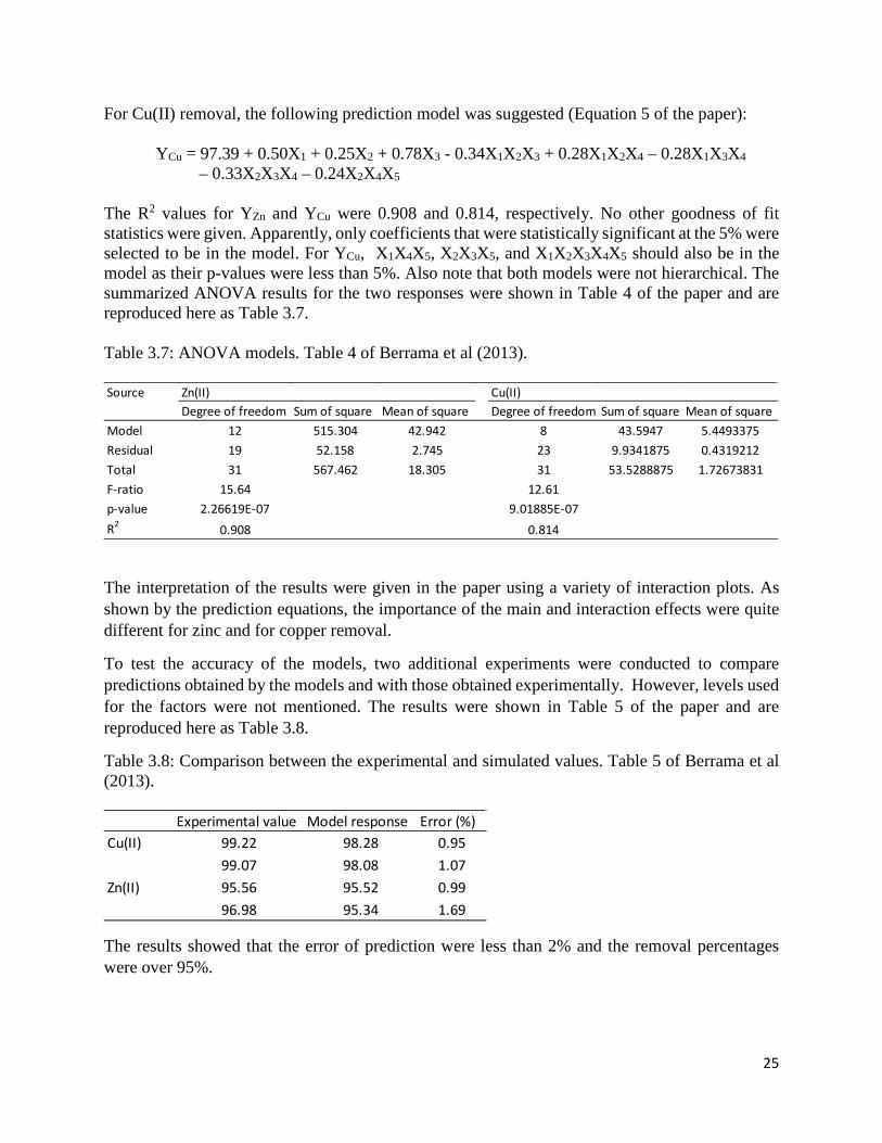
For Cu(II) removal, the following prediction model was suggested (Equation 5 of the paper):
YCu = 97.39 + 0.50X1 + 0.25X2 + 0.78X3 - 0.34X1X2X3 + 0.28X1X2X4 – 0.28X1X3X4 – 0.33X2X3X4 – 0.24X2X4X5
The R2 values for YZn and YCu were 0.908 and 0.814, respectively. No other goodness of fit statistics were given. Apparently, only coefficients that were statistically significant at the 5% were selected to be in the model. For YCu, X1X4X5, X2X3X5, and X1X2X3X4X5 should also be in the model as their p-values were less than 5%. Also note that both models were not hierarchical. The summarized ANOVA results for the two responses were shown in Table 4 of the paper and are reproduced here as Table 3.7. Table 3.7: ANOVA models. Table 4 of Berrama et al (2013).
The interpretation of the results were given in the paper using a variety of interaction plots. As shown by the prediction equations, the importance of the main and interaction effects were quite different for zinc and for copper removal.
To test the accuracy of the models, two additional experiments were conducted to compare predictions obtained by the models and with those obtained experimentally. However, levels used for the factors were not mentioned. The results were shown in Table 5 of the paper and are reproduced here as Table 3.8.
Table 3.8: Comparison between the experimental and simulated values. Table 5 of Berrama et al (2013).
The results showed that the error of prediction were less than 2% and the removal percentages were over 95%.
Source Zn(II) Cu(II)Degree of freedom Sum of square Mean of square Degree of freedom Sum of square Mean of square
Model 12 515.304 42.942 8 43.5947 5.4493375Residual 19 52.158 2.745 23 9.9341875 0.4319212Total 31 567.462 18.305 31 53.5288875 1.72673831F-ratio 15.64 12.61p-value 2.26619E-07 9.01885E-07R2 0.908 0.814
Experimental value Model response Error (%)Cu(II) 99.22 98.28 0.95
99.07 98.08 1.07Zn(II) 95.56 95.52 0.99
96.98 95.34 1.69
26
Case Study #3.3
Boubakri, A., Nawel Helali, Mohamed Tlili, and Mohamed Ben Amor (2014): Fluoride removal from diluted solutions by Donnan analysis using full factorial design. Korean Journal of Chemical Engineering, 31(3), pp. 461-466.
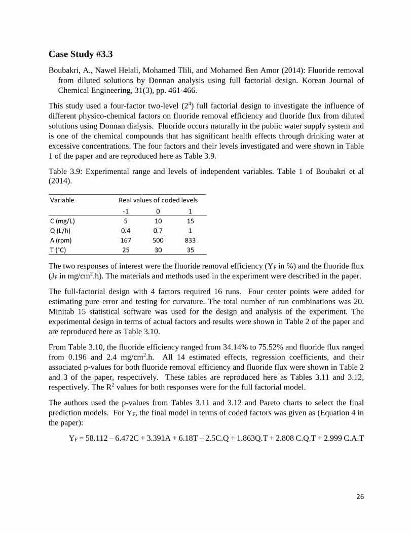
This study used a four-factor two-level (24) full factorial design to investigate the influence of different physico-chemical factors on fluoride removal efficiency and fluoride flux from diluted solutions using Donnan dialysis. Fluoride occurs naturally in the public water supply system and is one of the chemical compounds that has significant health effects through drinking water at excessive concentrations. The four factors and their levels investigated and were shown in Table 1 of the paper and are reproduced here as Table 3.9.
Table 3.9: Experimental range and levels of independent variables. Table 1 of Boubakri et al (2014).
The two responses of interest were the fluoride removal efficiency (YF in %) and the fluoride flux (JF in mg/cm2.h). The materials and methods used in the experiment were described in the paper.
The full-factorial design with 4 factors required 16 runs. Four center points were added for estimating pure error and testing for curvature. The total number of run combinations was 20. Minitab 15 statistical software was used for the design and analysis of the experiment. The experimental design in terms of actual factors and results were shown in Table 2 of the paper and are reproduced here as Table 3.10.
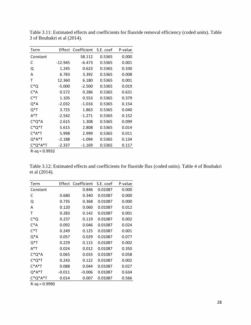
From Table 3.10, the fluoride efficiency ranged from 34.14% to 75.52% and fluoride flux ranged from 0.196 and 2.4 mg/cm2.h. All 14 estimated effects, regression coefficients, and their associated p-values for both fluoride removal efficiency and fluoride flux were shown in Table 2 and 3 of the paper, respectively. These tables are reproduced here as Tables 3.11 and 3.12, respectively. The R2 values for both responses were for the full factorial model.
The authors used the p-values from Tables 3.11 and 3.12 and Pareto charts to select the final prediction models. For YF, the final model in terms of coded factors was given as (Equation 4 in the paper):
YF = 58.112 – 6.472C + 3.391A + 6.18T – 2.5C.Q + 1.863Q.T + 2.808 C.Q.T + 2.999 C.A.T
Variable-1 0 1
C (mg/L) 5 10 15Q (L/h) 0.4 0.7 1A (rpm) 167 500 833T (°C) 25 30 35
Real values of coded levels

27
For JF, the final model in terms of coded factors was given as (Equation 5 in the paper):
JF = 0.846 + 0.340C + 0.367Q + 0.060A + 0.142T + 0.119C.Q + 0.046C.A + 0.124 C.T + 0.114Q.T + 0.122C.Q.T + 0.044 C.A.T No goodness of fit statistics were reported for these reduced equations. Also note that these equations were not hierarchical. There was no mention of whether curvature was tested as part of the analysis or if any regression assumptions checks were made.
Table 3.10: Full factorial design matrix for fluoride removal efficiency. Table 2 of Boukakri et al (2014).
Reanalysis of the data using Design-Expert 12 gave similar but not identical results. The standard errors of the estimated coefficients and associated p-values were quite different. However, in general the estimated regression coefficients were similar in magnitude and the models chosen by the authors gave good results.
Run C Q A T YF JF
(mg/L) (L/h) (rpm) (°C) (%) (mg/cm2.h)1 5 0.4 167 25 45.40 0.1962 15 0.4 167 25 52.27 0.6803 5 1 167 25 58.26 0.6904 15 1 167 25 34.14 1.0605 5 0.4 833 25 64.38 0.2706 15 0.4 833 25 50.64 0.6607 5 1 833 25 67.79 0.8008 15 1 833 25 42.58 1.2809 5 0.4 167 35 66.74 0.28410 15 0.4 167 35 47.92 0.63011 5 1 167 35 75.52 0.80012 15 1 167 35 57.96 1.95013 5 0.4 833 35 69.33 0.28014 15 0.4 833 35 63.24 0.83015 5 1 833 35 69.26 0.73016 15 1 833 35 64.81 2.40017 10 0.7 500 30 57.98 0.84018 10 0.7 500 30 60.49 0.92019 10 0.7 500 30 61.05 0.92020 10 0.7 500 30 56.48 0.850
28
Table 3.11: Estimated effects and coefficients for fluoride removal efficiency (coded units). Table 3 of Boubakri et al (2014).
Table 3.12: Estimated effects and coefficients for fluoride flux (coded units). Table 4 of Boubakri et al (2014).
Term Effect Coefficient S.E. coef P-valueConstant 58.112 0.5365 0.000C -12.945 -6.473 0.5365 0.001Q 1.245 0.623 0.5365 0.330A 6.783 3.392 0.5365 0.008T 12.360 6.180 0.5365 0.001C*Q -5.000 -2.500 0.5365 0.019C*A 0.572 0.286 0.5365 0.631C*T 1.105 0.553 0.5365 0.379Q*A -2.032 -1.016 0.5365 0.154Q*T 3.725 1.863 0.5365 0.040A*T -2.542 -1.271 0.5365 0.152C*Q*A 2.615 1.308 0.5365 0.099C*Q*T 5.615 2.808 0.5365 0.014C*A*T 5.998 2.999 0.5365 0.011Q*A*T -2.188 -1.094 0.5365 0.134C*Q*A*T -2.337 -1.169 0.5365 0.117R-sq = 0.9932
Term Effect Coefficient S.E. coef P-valueConstant 0.846 0.01087 0.000C 0.680 0.340 0.01087 0.000Q 0.735 0.368 0.01087 0.000A 0.120 0.060 0.01087 0.012T 0.283 0.142 0.01087 0.001C*Q 0.237 0.119 0.01087 0.002C*A 0.092 0.046 0.01087 0.024C*T 0.249 0.125 0.01087 0.001Q*A 0.057 0.029 0.01087 0.077Q*T 0.229 0.115 0.01087 0.002A*T 0.024 0.012 0.01087 0.350C*Q*A 0.065 0.033 0.01087 0.058C*Q*T 0.243 0.122 0.01087 0.002C*A*T 0.088 0.044 0.01087 0.027Q*A*T -0.011 -0.006 0.01087 0.634C*Q*A*T 0.014 0.007 0.01087 0.566R-sq = 0.9990

29
Case Study #3.4
Golshani, T., Jorjani, E., Chelgani S. Chehreh, Shafaei, S. Z., and Nafechi Y. Heidari (2013): Modeling and process optimization for microbial desulfurization of coal by using a two-level full factorial design. International Journal of Mining Science and Technology, 23, pp. 261-265.
This study used a five-factor two-level (25) full factorial design to model and optimize coal microbial desulfurization conditions from the Tabas coal preparation plant in Iran. The goals of the study were to determine the effects and interactions on the total sulfur reduction and to maximize the reduction of sulfur from high sulfur content coal samples. The five factors and their levels used in the experiment were shown in Table 2 of the paper and are reproduced here as Table 3.13.
Table 3.13: Variables, symbols, and levels used for full factorial design. Table 2 of Golshani et al (2013).
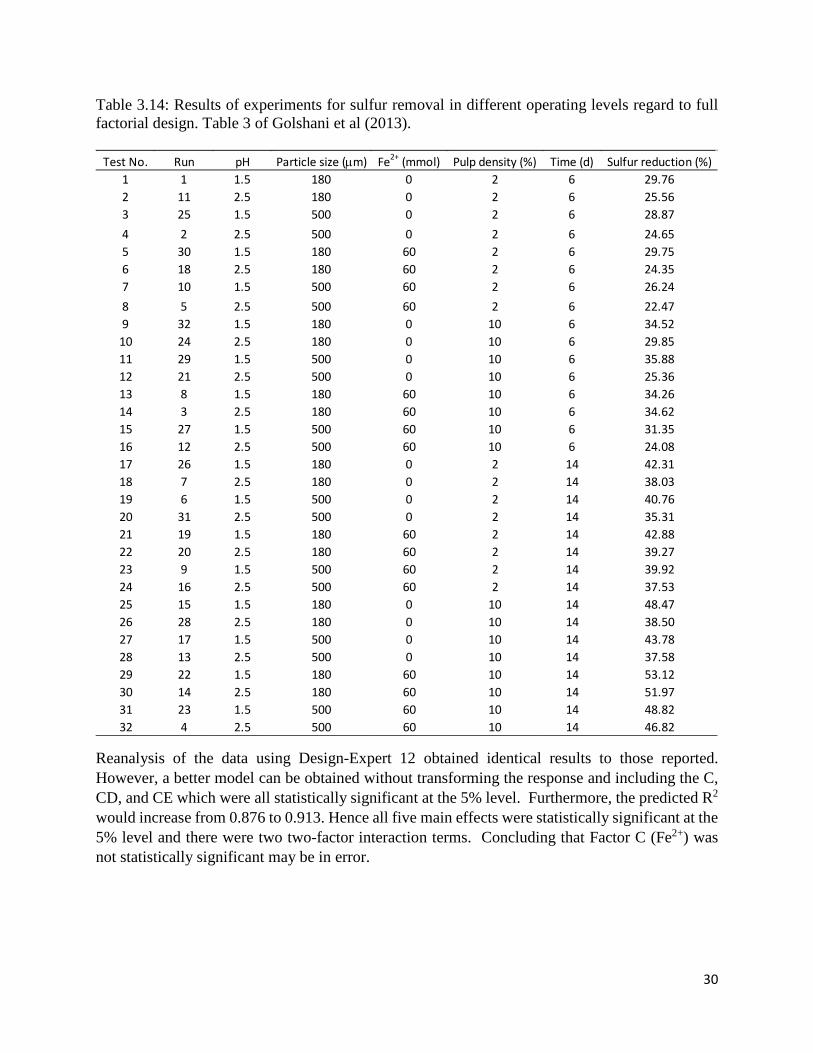
The response of interest was the sulfur reduction (%). The methods and materials used in the experiment were described in the paper. Design-Expert 7.0 statistical software was used for the design and analysis of the experiment. The full-factorial design with 5 factors required 32 runs. The experimental design in terms of actual factors and results were shown in Table 3 of the paper and are reproduced here as Table 3.14.
The response ranged from 22.47% to 53.12%. The authors used a half-normal plot of effects to select the significant effects for the prediction model. The final suggested model (Equation 3 in the paper) in actual factors was given as:
log10(sulfur reduction) = 1.4379 – 0.06128 pH – 1.18057 x 10⁻⁴ particle size + 8.44246 x 10⁻³ pulp density + 0.21607 time
The ANOVA results for the above reduced first order model were shown in Table 4 of the paper and are reproduced here as Table 3.15. The results were in log base 10 units. As can be seen from the ANOVA results, all terms were statistically significant at the 5% level. Factor C (Fe2+) was not statistically significant at the 5% level and no two-factor interaction terms were included. The goodness of fit statistics showed that this model had a R2 of 91.19% and a adjusted R2 of 89.89%.
Variable Symbol Lowe level Center level High level-1 0 1
pH A 1.5 2.0 2.5Particle size (µm) B 180 340 500Fe2+ (mmol) C 0 30 60Pulp density (%) D 2 6 10Leaching time (d) E 6 10 14
30
Table 3.14: Results of experiments for sulfur removal in different operating levels regard to full factorial design. Table 3 of Golshani et al (2013).
Reanalysis of the data using Design-Expert 12 obtained identical results to those reported. However, a better model can be obtained without transforming the response and including the C, CD, and CE which were all statistically significant at the 5% level. Furthermore, the predicted R2 would increase from 0.876 to 0.913. Hence all five main effects were statistically significant at the 5% level and there were two two-factor interaction terms. Concluding that Factor C (Fe2+) was not statistically significant may be in error.
Test No. Run pH Particle size (µm) Fe2+ (mmol) Pulp density (%) Time (d) Sulfur reduction (%)1 1 1.5 180 0 2 6 29.762 11 2.5 180 0 2 6 25.563 25 1.5 500 0 2 6 28.874 2 2.5 500 0 2 6 24.655 30 1.5 180 60 2 6 29.756 18 2.5 180 60 2 6 24.357 10 1.5 500 60 2 6 26.248 5 2.5 500 60 2 6 22.479 32 1.5 180 0 10 6 34.5210 24 2.5 180 0 10 6 29.8511 29 1.5 500 0 10 6 35.8812 21 2.5 500 0 10 6 25.3613 8 1.5 180 60 10 6 34.2614 3 2.5 180 60 10 6 34.6215 27 1.5 500 60 10 6 31.3516 12 2.5 500 60 10 6 24.0817 26 1.5 180 0 2 14 42.3118 7 2.5 180 0 2 14 38.0319 6 1.5 500 0 2 14 40.7620 31 2.5 500 0 2 14 35.3121 19 1.5 180 60 2 14 42.8822 20 2.5 180 60 2 14 39.2723 9 1.5 500 60 2 14 39.9224 16 2.5 500 60 2 14 37.5325 15 1.5 180 0 10 14 48.4726 28 2.5 180 0 10 14 38.5027 17 1.5 500 0 10 14 43.7828 13 2.5 500 0 10 14 37.5829 22 1.5 180 60 10 14 53.1230 14 2.5 180 60 10 14 51.9731 23 1.5 500 60 10 14 48.8232 4 2.5 500 60 10 14 46.82

31
Table 3.15: Analysis of variance for sulfur reduction. Table 4 of Golshani et al (23013).
The authors then used the optimization routine in Design-Expert 7 together with the developed model to determine the conditions that will maximize sulfur reduction. The optimum conditions obtained were pH of 1.5, particle size of 180 µm, iron sulfate concentration of 2.67 (mmol/L), pulp density of 10%, and bioleaching time of 14 days. The predicted sulfur reduction was 51.47%. The experimental result at these optimal conditions was 52.89%.
Since the iron sulfate concentration factor was not statistically significant according to the author’s model, it could have been set to 0 instead of 2.67.
Case Study #3.5
Khademi, A., Nafiseh G. Renani, Maryam Mofarrahi, Alireza Rangraz Jeddi, and Noordin M. Yusof (2013): The best location for speed bump installation using experimental design methodology. Promet – Traffic and Transportation, Vol. 25, No. 6, pp. 565-574.
This study used a four-factor two-level (24) full factorial design to determine the optimum location to install speed bumps before stopping points along a road to control traffic speeds through critical areas. Speed bumps are well-known traffic calming techniques used around the world. The factors and levels considered in this study are shown in Table 3.16.
Table 3.16: Factors and levels used in the speed bump installation experiment.
The response was supposed to be the speed at the stop point. However, due to the lack of a proper speed measurement instrument, the time in seconds taken between the bump and the stop point was taken as the response. The experimental procedure used was described in the paper. A two-level full factorial design with four factors would require 16 run combinations. The authors
Source Sum of squares df Mean square F value p-valueModel 0.320 4 0.079 69.89 <0.0001 SA-pH 0.030 1 0.030 26.50 <0.0001B-Particle size 0.011 1 0.011 10.07 0.0037D-Pulp density 0.036 1 0.036 32.18 <0.0001E-Time 0.240 1 0.240 210.82 <0.0001Residual 0.031 27 1.13E-03Cor total 0.350 31S: significant, CV=2.18%, R2=91.19%, Adj. R2=89.89%
Factor Symbol Low Level (-1) Mid Level (0) High Level (+1)Car weight (No. of passengers) A 1 3 5Car speed (km/h) B 10 20 30Distance (m) C 10 15 20Surface inclination (%) D 0 3.5 7

32
considered three replications for a total of 3 x 24 = 48 runs. Due to the large number of runs, the experiments were conducted over two days. Each day was considered as a block using I=ABCD as the block generator. Two center points were also added to each block to check for curvature. Hence, the total number of runs was 52.
Design-Expert 8 was used for the experimental design and analysis. The design and responses were shown in Table 2 of the paper and are reproduced here as Table 3.17.
Table 3.17: Response factors, which were measured in the performed actual experimental design. Table 2 of Khademi et al (2013).
From Table 3.17, there were 60 data points in total because three replications were also used for the center points. No explanation was given on how the center point results were used in the analysis as there should be only 52 points used in the analysis.
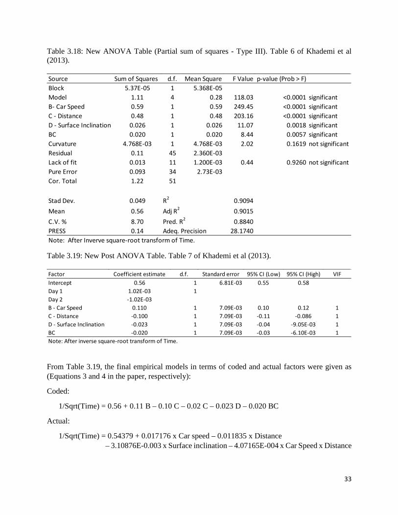
In the first round of analysis, the authors found that an inverse square-root transformation of the response was required to meet the assumptions of regression. The ANOVA results with only the statistically significant effects at the 5% level and the goodness of fit statistics were shown in Table 6 of the paper and are reproduced here as Table 3.18. The regression coefficient estimates and associated standard errors were shown in Table 7 of the paper and are reproduced here as Table 3.19.
Std
Trea
tmen
t Co
mbi
natio
n
ABCD
Fac
toria
l Ef
fect A: Car weight
(No. of passengers)
B: Car Speed (km/h)
C: Distance
(m)
D: Surface Inclination
(%)R1 R2 R3 Total Average
Standard Deviation
1 (1) + 1 10 10 0 2.18 4.90 3.26 10.34 3.45 1.372 a - 5 10 10 0 3.05 3.69 3.35 10.09 3.36 0.323 b - 1 30 10 0 1.20 1.35 1.68 4.23 1.41 0.254 ab + 5 30 10 0 1.36 1.26 1.71 4.33 1.44 0.245 c - 1 10 20 0 4.31 7.76 6.56 18.63 6.21 1.756 ac + 5 10 20 0 4.41 7.95 7.72 20.08 6.69 1.987 bc + 1 30 20 0 3.08 3.05 3.29 9.42 3.14 0.138 abc - 5 30 20 0 3.13 3.16 3.37 9.66 3.22 0.139 d - 1 10 10 7 4.34 2.79 3.91 11.04 3.68 0.80
10 ad + 5 10 10 7 3.53 4.27 3.87 11.67 3.89 0.3711 bd + 1 30 10 7 1.65 1.66 1.96 5.27 1.76 0.1812 abd - 5 30 10 7 1.70 1.58 2.14 5.42 1.81 0.2913 cd + 1 10 20 7 8.12 8.42 8.64 25.18 8.39 0.2614 acd - 5 10 20 7 5.71 8.93 10.28 24.92 8.31 2.3515 bcd - 1 30 20 7 3.45 3.18 3.05 9.68 3.23 0.2016 abcd + 5 30 20 7 3.20 3.24 3.46 9.90 3.30 0.1417 CP 0 3 20 15 3.5 2.79 3.41 3.44 9.64 3.21 0.3718 CP 0 3 20 15 3.5 3.46 5.13 4.29 12.88 4.29 0.8419 CP 0 3 20 15 3.5 3.05 3.41 3.14 9.60 3.20 0.1920 CP 0 3 20 15 3.5 4.53 3.41 2.96 10.90 3.63 0.81
Factors No. of replicates (Time (s))
33
Table 3.18: New ANOVA Table (Partial sum of squares - Type III). Table 6 of Khademi et al (2013).
Table 3.19: New Post ANOVA Table. Table 7 of Khademi et al (2013).
From Table 3.19, the final empirical models in terms of coded and actual factors were given as (Equations 3 and 4 in the paper, respectively):
Coded:
1/Sqrt(Time) = 0.56 + 0.11 B – 0.10 C – 0.02 C – 0.023 D – 0.020 BC
Actual:
1/Sqrt(Time) = 0.54379 + 0.017176 x Car speed – 0.011835 x Distance – 3.10876E-0.003 x Surface inclination – 4.07165E-004 x Car Speed x Distance
Source Sum of Squares d.f. Mean Square F Value p-value (Prob > F)Block 5.37E-05 1 5.368E-05Model 1.11 4 0.28 118.03 <0.0001 significantB- Car Speed 0.59 1 0.59 249.45 <0.0001 significantC - Distance 0.48 1 0.48 203.16 <0.0001 significantD - Surface Inclination 0.026 1 0.026 11.07 0.0018 significantBC 0.020 1 0.020 8.44 0.0057 significantCurvature 4.768E-03 1 4.768E-03 2.02 0.1619 not significantResidual 0.11 45 2.360E-03Lack of fit 0.013 11 1.200E-03 0.44 0.9260 not significantPure Error 0.093 34 2.73E-03Cor. Total 1.22 51
Stad Dev. 0.049 R2 0.9094Mean 0.56 Adj R2 0.9015C.V. % 8.70 Pred. R2 0.8840PRESS 0.14 Adeq. Precision 28.1740Note: After Inverve square-root transform of Time.
Factor Coefficient estimate d.f. Standard error 95% CI (Low) 95% CI (High) VIFIntercept 0.56 1 6.81E-03 0.55 0.58Day 1 1.02E-03 1Day 2 -1.02E-03B - Car Speed 0.110 1 7.09E-03 0.10 0.12 1C - Distance -0.100 1 7.09E-03 -0.11 -0.086 1D - Surface Inclination -0.023 1 7.09E-03 -0.04 -9.05E-03 1BC -0.020 1 7.09E-03 -0.03 -6.10E-03 1Note: After inverse square-root transform of Time.
34
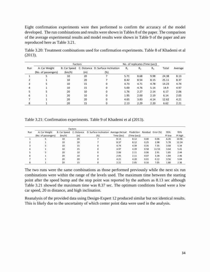
Eight confirmation experiments were then performed to confirm the accuracy of the model developed. The run combinations and results were shown in Tables 8 of the paper. The comparison of the average experimental results and model results were shown in Table 9 of the paper and are reproduced here as Table 3.21.
Table 3.20: Treatment combinations used for confirmation experiments. Table 8 of Khademi et al (2013).
Table 3.21: Confirmation experiments. Table 9 of Khademi et al (2013).
The two runs were the same combinations as those performed previously while the next six run combinations were within the range of the levels used. The maximum time between the starting point after the speed bump and the stop point was reported by the authors as 8.13 sec although Table 3.21 showed the maximum time was 8.37 sec. The optimum conditions found were a low car speed, 20 m distance, and high inclination.
Reanalysis of the provided data using Design-Expert 12 produced similar but not identical results. This is likely due to the uncertainty of which center point data were used in the analysis.
Run A: Car Weight B: Car Speed C: Distance D: Surface Inclination R1 R2 R3 Total Average(No. of passengers) (km/h) (m) (%)
1 5 10 20 7 5.71 8.68 9.98 24.38 8.132 1 10 20 7 8.42 8.54 8.15 25.11 8.373 5 10 15 0 4.73 4.71 4.78 14.23 4.744 1 10 15 0 5.00 4.76 5.14 14.9 4.975 5 20 10 0 1.76 2.27 2.14 6.17 2.066 1 20 10 0 1.95 2.00 2.19 6.14 2.057 1 20 20 0 4.65 3.83 4.14 12.62 4.218 1 20 15 0 2.13 2.29 2.20 6.62 2.21
No. of replicates (Time (sec))Factors
Run A: Car Weight B: Car Speed C: Distance D: Surface Inclination Average (Actual Prediction Residual Error (%) 95% 95%(No. of passengers) (km/h) (m) (%) Time (Sec) (Time (sec)) PI low PI high
1 5 10 20 7 8.13 8.12 0.00 0.06 6.26 10.962 1 10 20 7 8.37 8.12 0.25 2.98 5.78 12.243 5 10 15 0 4.74 4.39 0.35 7.35 3.68 5.344 1 10 15 0 4.97 4.39 0.58 11.53 3.64 5.415 5 20 10 0 2.06 2.11 0.06 2.91 1.85 2.446 1 20 10 0 2.05 2.11 0.07 3.28 1.84 2.467 1 20 20 0 4.21 4.20 0.01 0.12 3.56 5.048 1 20 15 0 2.21 2.05 0.16 7.05 1.80 2.36
Factors

35
Case Study #3.6
Mtaallah, S., Ikhlass Marzouk, and Bechir Hamrouni (2018): Factorial experimental design applied to adsorption of cadmium on activated alumina. Journal of Water Reuse and Desalination, 08.1, pp. 76-85.
In this study a four-factor two-level (24) full factorial design was used to investigate the influence of four factors on the removal efficiency of cadmium from aqueous solutions and industrial effluents by adsorption on activated alumina. Cadmium, a toxic heavy metal, adversely affects humans, animals, and plants. The materials and methods used in the experiment were described in the paper. The factors and levels used in the experiment were shown in Table 3 of the paper and are reproduced here as Table 3.22.
Table 3.22: Experimental ranges and levels of the factors studied in the factorial design. Table 3 of Mtaallah et al (2018).
The response of interest was the percentage removal of cadmium II (%Cd) as defined in the paper. Minitab 16 statistical software was used for the design and analysis of the experiment. The full-factorial design with 4 factors required 16 runs. Two center points were added to test for curvature and provide a measure of pure error. The experimental design in terms of actual factors and results were shown in Table 4 of the paper and are reproduced here as Table 3.23. The response ranged from 16.24% to 99.09%.
The reduced ANOVA results were shown in Table 5 of the paper and are reproduced here as Table 3.24. No goodness of fit statistics were given. The model representing Cd(II) removal was expressed as (Equation 3 of the paper):
%Cd = 63.25 + 14.67X1 – 20.23X2 – 5.17X3 + 13.54X4 + 2.3X1X2 + 3.45X1X3 + 0.89X1X4 + 0.83X2X3 + 0.64X3X4 + 3.29X2X4. As can be seen from Table 3.23, only factors A, B, and D were statistically significant at the 5% level, all other terms could have been left out of the model.
Reanalysis of the data using Design-Expert 12 showed that the model suggested by the authors had a predicted R2 of -0.1036 indicating that the model was no better than using the overall mean response. Furthermore, the lack of fit was also statistically significant and a highly statistically significant term (p-value <0.0001), ABD, was not included in the model.
Variables Factors Low level High levelX1 Dose AA (g) (A) 0.5 1.5X2 Initial Cd(II) concentration ([Cd], mg/L) (B) 10 100X3 pH (pH) (C) 5 8X4 Temperature (T, °C) (D) 10 40

36
Table 3.23: Studied parameters in their reduced and normal forms. Table 4 of Mtaallah et al (2018).
Table 3.24: ANOVA of the 24 design. Table 5 of Mtaallah et al (2018).
The authors concluded that the highest percentage removal of cadmium was obtained at a temperature of 40C, adsorbent dose of 1.5 g, and initial cadmium concentration of 10mg/L.
Experiment A X1 B X2 C X3 D X4 %Cd1 0.5 -1 10 -1 5 -1 10 -1 68.382 1.5 1 10 -1 5 -1 10 -1 94.623 0.5 -1 100 1 5 -1 10 -1 23.344 1.5 1 100 1 5 -1 10 -1 35.785 0.5 -1 10 -1 8 1 10 -1 35.786 1.5 1 10 -1 8 1 10 -1 94.137 0.5 -1 100 1 8 1 10 -1 16.248 1.5 1 100 1 8 1 10 -1 29.839 0.5 -1 10 -1 5 -1 40 1 95.88
10 1.5 1 10 -1 5 -1 40 1 99.0911 0.5 -1 100 1 5 -1 40 1 41.2212 1.5 1 100 1 5 -1 40 1 89.0813 0.5 -1 10 -1 8 1 40 1 84.4314 1.5 1 10 -1 8 1 40 1 95.515 0.5 -1 100 1 8 1 40 1 23.3416 1.5 1 100 1 8 1 40 1 85.7517 1 0 55 0 6.5 0 25 0 73.5418 1 0 55 0 6.5 0 25 0 73.21
Term Sum of Squares Degrees of freedom Mean square F-value p-valueA 3443.34 1 3443.340 10.25589 0.023929B 6548.05 1 6548.050 19.50316 0.006916C 428.9 1 428.900 1.27748 0.309653D 2933.31 1 2933.310 8.73676 0.031672A X B 85.47 1 85.470 0.25457 0.635319A X C 190.58 1 190.580 0.56763 0.485145A X D 12.92 1 12.920 0.03849 0.852180B X C 11.26 1 11.260 0.03353 0.861912B X D 173.32 1 173.320 0.51622 0.504623C X D 6.68 1 6.680 0.01990 0.893317Error 1678.71 5 335.743Total sum of squares 15512.54 15

37
Case Study #3.7
Nasirabadi, P. S., M. Jabbari, and J. H. Hattel (2017): CFD simulation and statistical analysis of moisture transfer into an electronic enclosure. Applied Mathematical Modelling, 44, pp. 246-260.
This study used a four-factor two-level (24) full factorial design and computational fluid dynamics (CFD) to investigate the moisture transfer into a typical electronic enclosure. The factors and levels investigated were shown in Table 2 of the paper and are reproduced here as Table 3.25. The CFD simulations were conducted using the COMSOL Multiphysics version 5.1 software package. Both isothermal and non-isothermal studies were carried out using the package. The geometry of the electronic enclosure and the equations used in the modelling were described in the paper.
Table 3.25: The studied ranges of the parameters in the factorial design. Table 2 of Nasirabadi et al (2017).
The main response of interest was the diffusion time of moisture into the enclosure at constant ambient temperature and relative humidity. The four-factor full factorial design with two levels required 16 run combinations. A center point was added to check for curvature. Note that only one center point was added because this was a computer based experiment with no random error. The software used for experimental design and statistical analysis was not reported in the paper. The experimental design and results were shown in Table 4 of the paper and are reproduced here as Table 3.26. Preliminary analysis showed that the response needed a logarithmic transformation to meet the assumptions of regression. The ANOVA results after a log-transform (base 10) of the response were shown in Table 5 of the paper and reproduced here as Table 3.27. Table 5 in the paper was wrongly captioned. The caption should read “ANOVA results” and should not be identical to Table 4 of the paper. The ANOVA results showed that only factors A, B and D were statistically significant at the 5% level and curvature was also statistically significant. The proposed regression model in terms of actual factors was (Equation 17 of the paper): Log(Response [s]) = 7.52153 + 0.022926 x L [mm] – 0.39190 x R [mm] – 8.03937 x 10⁻³ x RH [%] The goodness of fit statistics were given as R2 = 0.9363 and adjusted R2 = 0.9216.
Factor Notification Coded symbol Low level High level UnitLength of the opening (or tube) L A 2.00 50.00 [mm]Radius of the opening R B 0.50 5.00 [mm]Temperature T C 273.15 333.15 [K]Initial RH RH D 40.00 80.00 [%]

38
Table 3.26: The factorial design table for the factors and the responses. Table 4 of Nasirabadi et al (2017).
Table 3.27: The ANOVA table for the response. Table 5 of Nasirabadi et al (2017).
Reanalysis of the data using Design-Expert 12 gave practically identical ANOVA results to those reported but the intercept term in the regression equation was 7.47745 instead of the reported 7.52153. The R2 and adjusted R2 values were 0.9633 and 0.9541, respectively which were a little larger than those reported. Since the curvature was statistically significant at the 5% level, a better fit to the data would likely be obtained using a response surface model.
Case # A [mm] B [mm] C [K] D [%] Response (diffusion time) [s]1 2 0.5 273.15 40 8,500,000.00 2 50 0.5 273.15 40 208,000,000.00 3 2 5 273.15 40 143,000.00 4 50 5 273.15 40 1,474,000.00 5 2 0.5 333.15 40 6,210,000.00 6 50 0.5 333.15 40 149,450,000.00 7 2 5 333.15 40 464,000.00 8 50 5 333.15 40 1,544,000.00 9 2 0.5 273.15 80 4,892,000.00 10 50 0.5 273.15 80 166,460,000.00 11 2 5 273.15 80 108,000.00 12 50 5 273.15 80 1,095,000.00 13 2 0.5 333.15 80 3,815,000.00 14 50 0.5 333.15 80 28,500,000.00 15 2 5 333.15 80 72,000.00 16 50 5 333.15 80 880,000.00 17 26 2.75 303.15 60 18,318,000.00
Source Sum of Degree of Mean F-value p-valuesquares freedom square (Prob>F)
Model 17.7 3 5.90 104.85 <0.0001 SignificantA 4.84 1 4.84 86.09 <0.0001 SignificantB 12.44 1 12.44 221.11 <0.0001 SignificantD 0.41 1 0.41 7.35 0.0189 SignificantCurvature 0.53 1 0.53 9.39 0.0098 SignificantResidual 0.68 12 0.056Total 18.90 16

39
Case Study #3.8
Ridzuan, N., F. Adam, and Z. Yaacob (2016): Screening of factor influencing wax deposition using full factorial experimental design. Petroleum Science and Technology, Vol. 34, No. 1, pp. 84-90.
This study used a four-factor two-level (24) full factorial design to investigate the rate of wax deposition of Malaysia crude oil under the influence of four parameters or factors. The factors were the speed of rotation of the impeller, the cold finger temperature, experimental duration, and inhibitor concentration. The factors and levels used for the experiment are summarized in Table 3.28. The experimental setup and materials used were described in the paper.
Table 3.28: Factors and levels used in the wax deposition experiment.
The response of interest was the wax deposition (g). The 24 experiment required 16 run combinations and three center points were added to check for curvature and as a measure of pure error. Hence a total of 19 runs was used. Design-Expert 7.1.6 software was used for the experimental design and statistical analysis.
The experimental design in coded and actual factors, and results were shown in Table 1 of the paper and are reproduced here as Table 3.29. Wax deposition ranged from 0.75 g to 3.0 g. The partial ANOVA results were shown in Table 2 of the paper and are reproduced here as Table 3.30.
The authors proposed the following regression model for wax deposition (in coded factors) (Equation 2 of the paper):
Wax deposit = 1.68 + 0.12 – 0.60 + 0.34 C – 0.059 D + 0.059 AD – 0.12 BC – 0.053 BD
The R2 value was reported as 0.9795. No other goodness of fit statistics were reported. Note that from the ANOVA table, effect D, AD, and BD were not statistically significant at the 5% level. Furthermore, the curvature was statistically significant at the 5% level. The authors did not discuss the statistically significant curvature term and did not provide reasons for including the three insignificant terms in the model. This experiment should be followed up with a response surface experiment to account for the curvature effect.
Factor SymbolLow level (-1) Mid level (0) High level (+1)
Speed of rotation, rpm A 0 300 600Cold finger temperature, °C B 5 10 15Experimental duration, h C 2 13 24Inhibitor concentration, ppm D 200 2600 5000
Levels

40
Table 3.29: Results for the screening design according to standard order. Table 1 of Ridzuan et al (2016).
Table 3.30: Analysis of variance. Table 2 of Ridzuan et al (2016).
A B C DUncoded/ Uncoded/ Uncoded/ Uncoded/ Wax deposit, g
Standard order coded coded coded coded1 0 (-1) 5 2 200 1.902 600 (+1) 5 2 200 1.803 0 (-1) 15 2 200 0.804 600 (+1) 15 2 200 1.005 0 (-1) 5 24 200 2.656 600 (+1) 5 24 200 2.807 0 (-1) 15 24 200 1.408 600 (+1) 15 24 200 1.609 0 (-1) 5 2 5000 1.50
10 600 (+1) 5 2 5000 2.1011 0 (-1) 15 2 5000 0.7512 600 (+1) 15 2 5000 0.9013 0 (-1) 5 24 5000 2.5014 600 (+1) 5 24 5000 3.0015 0 (-1) 15 24 5000 1.0516 600 (+1) 15 24 5000 1.2017 300 (0) 10 13 2600 1.4018 300 (0) 10 13 2600 1.5019 300 (0) 10 13 2600 1.45
Factors
Sum of Mean F p-value %Source squares DF square value Prob>F ContributionModel 8.14 7 1.16 68.220 <0.0001 A - Speed of rotation 0.21 1 0.21 12.540 0.0053 2.54 B - Cold finger temperature 5.70 1 5.70 334.290 <0.0001 67.65 C - Experimental duration 1.86 1 1.86 108.870 <0.0001 22.03 D - Inhibitor concentration 0.06 1 0.06 3.310 0.099 0.67AD 0.06 1 0.06 3.310 0.099 0.67BC 0.21 1 0.21 12.540 0.0053 2.54BD 0.05 1 0.05 2.650 0.1347 0.54Curvature 0.11 1 0.11 6.600 0.0279Residual 0.17 10 0.017Lack of fit 0.16 8 0.02 4.350 0.2003Pur error 9.27E-03 2 4.63E-03Cor total 8.43 18
41
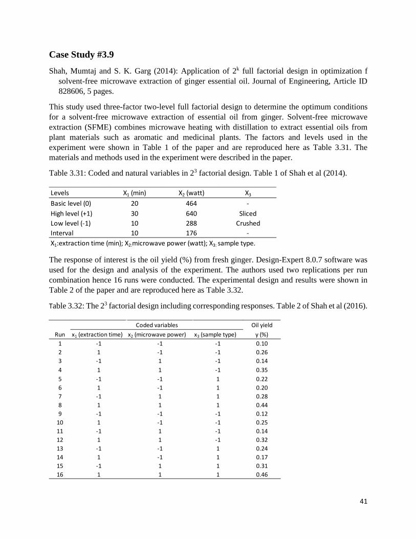
Case Study #3.9
Shah, Mumtaj and S. K. Garg (2014): Application of 2k full factorial design in optimization f solvent-free microwave extraction of ginger essential oil. Journal of Engineering, Article ID 828606, 5 pages.
This study used three-factor two-level full factorial design to determine the optimum conditions for a solvent-free microwave extraction of essential oil from ginger. Solvent-free microwave extraction (SFME) combines microwave heating with distillation to extract essential oils from plant materials such as aromatic and medicinal plants. The factors and levels used in the experiment were shown in Table 1 of the paper and are reproduced here as Table 3.31. The materials and methods used in the experiment were described in the paper.
Table 3.31: Coded and natural variables in 23 factorial design. Table 1 of Shah et al (2014).
The response of interest is the oil yield (%) from fresh ginger. Design-Expert 8.0.7 software was used for the design and analysis of the experiment. The authors used two replications per run combination hence 16 runs were conducted. The experimental design and results were shown in Table 2 of the paper and are reproduced here as Table 3.32.
Table 3.32: The 23 factorial design including corresponding responses. Table 2 of Shah et al (2016).
Levels X1 (min) X2 (watt) X3
Basic level (0) 20 464 -High level (+1) 30 640 SlicedLow level (-1) 10 288 CrushedInterval 10 176 -X1:extraction time (min); X2:microwave power (watt); X3: sample type.
Oil yieldRun x1 (extraction time) x2 (microwave power) x3 (sample type) y (%)
1 -1 -1 -1 0.102 1 -1 -1 0.263 -1 1 -1 0.144 1 1 -1 0.355 -1 -1 1 0.226 1 -1 1 0.207 -1 1 1 0.288 1 1 1 0.449 -1 -1 -1 0.12
10 1 -1 -1 0.2511 -1 1 -1 0.1412 1 1 -1 0.3213 -1 -1 1 0.2414 1 -1 1 0.1715 -1 1 1 0.3116 1 1 1 0.46
Coded variables
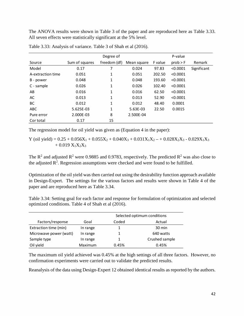
42
The ANOVA results were shown in Table 3 of the paper and are reproduced here as Table 3.33. All seven effects were statistically significant at the 5% level.
Table 3.33: Analysis of variance. Table 3 of Shah et al (2016).
The regression model for oil yield was given as (Equation 4 in the paper):
Y (oil yield) = 0.25 + 0.056X1 + 0.055X2 + 0.040X3 + 0.031X1X2 – + 0.028X2X3 - 0.029X1X3 + 0.019 X1X2X3
The R2 and adjusted R2 were 0.9885 and 0.9783, respectively. The predicted R2 was also close to the adjusted R2. Regression assumptions were checked and were found to be fulfilled. Optimization of the oil yield was then carried out using the desirability function approach available in Design-Expert. The settings for the various factors and results were shown in Table 4 of the paper and are reproduced here as Table 3.34. Table 3.34: Setting goal for each factor and response for formulation of optimization and selected optimized conditions. Table 4 of Shah et al (2016).
The maximum oil yield achieved was 0.45% at the high settings of all three factors. However, no confirmation experiments were carried out to validate the predicted results.
Reanalysis of the data using Design-Expert 12 obtained identical results as reported by the authors.
Degree of P-valueSource Sum of squares freedom (df) Mean square F value prob > F RemarkModel 0.17 7 0.024 97.83 <0.0001 SignificantA-extraction time 0.051 1 0.051 202.50 <0.0001B - power 0.048 1 0.048 193.60 <0.0001C - sample 0.026 1 0.026 102.40 <0.0001AB 0.016 1 0.016 62.50 <0.0001AC 0.013 1 0.013 52.90 <0.0001BC 0.012 1 0.012 48.40 0.0001ABC 5.625E-03 1 5.63E-03 22.50 0.0015Pure error 2.000E-03 8 2.500E-04Cor total 0.17 15
Factors/response Goal Coded ActualExtraction time (min) In range 1 30 minMicrowave power (watt) In range 1 640 wattsSample type In range 1 Crushed sampleOil yield Maximum 0.45% 0.45%
Selected optimum conditions

43
Case Study #3.10
Yusoff, N. H. N., M. J. Ghazali, M. C. Isa, A. R. Daud, A. Muchtar, and S.M. Forghani (2012): Optimization of plasma spray parameters on the mechanical properties of agglomerated Al2O3-13%TiO2 coated mild steel. Materials and Design, 39, pp. 504-508.
This study used a three-factor two level (23) full factorial design to investigate the effect of plasma spray parameters of deposited agglomerated nano Al2O3-13%TiO2 powders on commercial marine-grade mild steels. The parameters or factors and levels used in the experiment were shown in Table 1 of the paper and are reproduced here as Table 3.35. The experimental procedures and materials used in the experiment were described in the paper.
Table 3.35: Experimental range and levels of independent parameters for plasma spray coating. Table 1 of Yusoff et al (2012).
Three responses of interest were – Y1, microhardness; Y2, specific wear rate; and Y3, surface roughness. Design-Expert 6.0.10 software was used for the design and analysis of the experiment. The authors added one center point to the 23 design resulting in 9 runs. The experimental design and results were shown in Table 2 of the paper and are reproduced here as Table 3.36.
Table 3.36: Full-factorial design for plasma spray experiment. Table 2 of Yusoff et al (2012).
The partial ANOVA results and estimated regressions coefficients in coded units were shown in Table 3 of the paper and are reproduced here as Table 3.37.
Independent parametersLow (-1) Central point (0) High (+1)
Primary gas pressure (X1) psi 40 80 120Carrier gas pressure (X2) psi 20 32.5 45Powder feed rate (X3) rpm 1 2 3
Range (coded level)
Run X1 X2 X3 Y1 Y2 Y3
1 -1 1 1 350 0.0240 9.882 1 1 1 555 0.0068 9.523 -1 1 -1 375 0.0176 9.194 -1 -1 1 413 0.0219 7.495 1 -1 1 1057 0.0023 8.366 1 1 -1 958 0.0012 11.297 1 -1 -1 714 0.0050 10.008 -1 -1 -1 965 0.0004 7.439 0 0 0 473 0.0499 9.63

44
Table 3.37: Full 23 factorials design (Coefficient are given in coded unit). Table 3 of Yusoff et al (2012).
The final regression models in coded factors with statistically significant terms at the 5% level were given as (Equations 2 to 4 of the paper):
Y1 = microhardness = 663.13 – 260.38 X1
Y2 = specific wear rate = 0.015 + 0.013 X1
Y3 = surface roughness = 9.16 + 0.45 X2 – 0.93 X1X3 + 0.63 X2X3
Goodness of fit statistics for these models were not reported. Also note from Table 3.37, Y3, X2 was not statistically significant at the 5% level.
The authors found that the optimum properties of the coatings with the best wear resistance, surface roughness, and microhardness occurred at the lowest primary pressure of 40 psi, carrier gas pressure of 20 psi, and the highest powder feed rate of 3 rpm.
Reanalysis of the given data using Design-Expert 12 did not reproduce the same ANOVA results or estimated regression coefficients. Hence, the results reported may not be valid.
Term SS Coefficient P value(a) for Y1
X1 5.60E+05 -264.88 0.0004
(b) For Y2
X1 1.37E-03 0.013 0.0122
(c) For Y3
X1 0.097 -0.11 0.42X2 1.59 0.45 0.06X2 0.41 0.23 0.18X1X2 6.93 -0.93 0.01X2X3 3.18 0.63 0.03
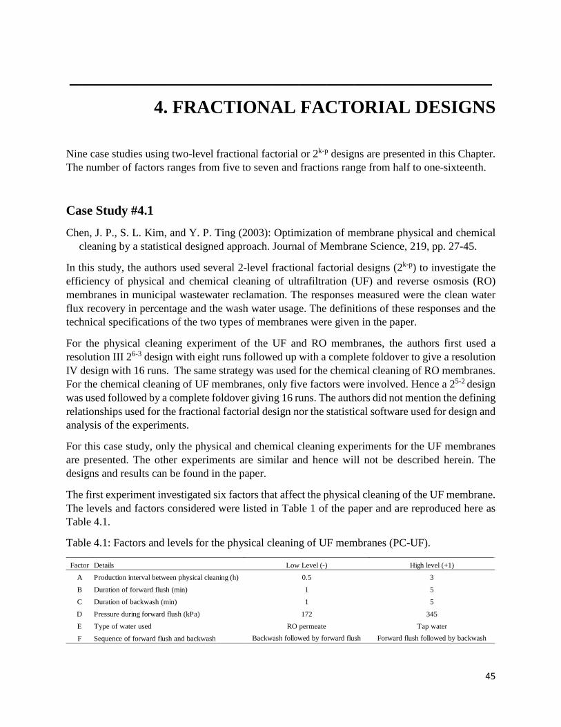
45
______________________________________________ 4. FRACTIONAL FACTORIAL DESIGNS
Nine case studies using two-level fractional factorial or 2k-p designs are presented in this Chapter. The number of factors ranges from five to seven and fractions range from half to one-sixteenth.
Case Study #4.1
Chen, J. P., S. L. Kim, and Y. P. Ting (2003): Optimization of membrane physical and chemical cleaning by a statistical designed approach. Journal of Membrane Science, 219, pp. 27-45.
In this study, the authors used several 2-level fractional factorial designs (2k-p) to investigate the efficiency of physical and chemical cleaning of ultrafiltration (UF) and reverse osmosis (RO) membranes in municipal wastewater reclamation. The responses measured were the clean water flux recovery in percentage and the wash water usage. The definitions of these responses and the technical specifications of the two types of membranes were given in the paper.
For the physical cleaning experiment of the UF and RO membranes, the authors first used a resolution III 26-3 design with eight runs followed up with a complete foldover to give a resolution IV design with 16 runs. The same strategy was used for the chemical cleaning of RO membranes. For the chemical cleaning of UF membranes, only five factors were involved. Hence a 25-2 design was used followed by a complete foldover giving 16 runs. The authors did not mention the defining relationships used for the fractional factorial design nor the statistical software used for design and analysis of the experiments.
For this case study, only the physical and chemical cleaning experiments for the UF membranes are presented. The other experiments are similar and hence will not be described herein. The designs and results can be found in the paper.
The first experiment investigated six factors that affect the physical cleaning of the UF membrane. The levels and factors considered were listed in Table 1 of the paper and are reproduced here as Table 4.1.
Table 4.1: Factors and levels for the physical cleaning of UF membranes (PC-UF).
Factor Details Low Level (-) High level (+1)
A Production interval between physical cleaning (h) 0.5 3
B Duration of forward flush (min) 1 5
C Duration of backwash (min) 1 5
D Pressure during forward flush (kPa) 172 345
E Type of water used RO permeate Tap water
F Sequence of forward flush and backwash Backwash followed by forward flush Forward flush followed by backwash

46
The experimental design, a 26-3 design with a complete foldover, and results were shown in Table 2 of the paper. It is adapted here in Table 4.2. The two responses CWF recovery (%) and wash water usage are labelled here as y1 and y2, respectively.
Table 4.3: Experimental design and results in physical cleaning of UF (PC-UF). Adapted from Table 2 of Chen et al (2003).
The authors used the normal probability plot of effects to select the statistically significant effects. No ANOVA results were shown and the significance level was not mentioned. From the normal effects plots, the following models (in coded values) were suggested for CWF recovery % (y1), and wash water usage (y2) (these were Equations 5a and 5b in the paper):
y1 = 85.17 – 4.090 x1 + 2.749 x3 – 1.611 x4 + 1.801 x1x3
y2 = 0.309 – 0.209 x1 + 0.131 x2 + 0.070 x3 – 0.016 x1 x2 – 0.026 x1x3
where, the variables x1, x2, x3 and x4 represent values of A, B, C, and D, respectively. The terms x1x2 and x1x3 represent the interaction between A and B, and A and C, respectively. No goodness of fit statistics were given.
For the chemical cleaning of UF membranes, five factors were studied. The factors and levels are shown in Table 4.3.
Run CWF % WWU
A B C D E F y1 y2
1 -1 -1 -1 1 1 1 82.54 0.15
2 1 -1 -1 -1 -1 1 80.56 0.03
3 -1 1 -1 -1 1 -1 92.89 0.32
4 1 1 -1 1 -1 -1 75.80 0.08
5 -1 -1 1 1 -1 -1 88.73 0.346 1 -1 1 -1 1 -1 86.34 0.087 -1 1 1 -1 -1 1 94.89 0.488 1 1 1 1 1 1 87.19 0.129 1 1 1 -1 -1 -1 88.02 0.11
10 -1 1 1 1 1 -1 87.94 0.5811 1 -1 1 1 -1 1 82.21 0.0812 -1 -1 1 -1 1 1 88.73 0.3413 1 1 -1 -1 1 1 73.03 0.0914 -1 1 -1 1 -1 1 87.24 0.3415 1 -1 -1 1 1 -1 76.18 0.0316 -1 -1 -1 -1 -1 -1 90.48 0.10
Factors

47
Table 4.3: Factors and levels for the chemical cleaning of UF membranes (CC-UF).
The authors first used a 25-2 design followed by a complete foldover. The experimental design and results were shown in Table 4 of the paper and are reproduced here as Table 4.4. For this experiment only one response, the CWF recovery % was measured. It is labelled as y5 in Table 4.4.
Table 4.4: Experimental design and results of chemical cleaning of UF (CC-UF). Adapted from Table 4 of Chen et al (2003).
From the normal probability plot of effects, the authors suggested the follow regression equation for CWF recovery % (y5) (Equation 7 in the paper):
y5 = 89.15 – 3.409 x2 + 5.000 x3 – 3.436 x5 – 2.076 x2x3
where the factors involved are B(x2), C(x3), and E(x5). No ANOVA results or goodness of fit statistics were given.
Overall, the authors found that the application of factorial design to optimize physical and chemical cleaning of both UF and RO membranes was successful.
Factor Details Low Level (-) High level (+1)A Recirculation duration of high pH cleaning (min) 30 60B Concentration of high pH cleaning solution (%) 0.5 1C Temperature of high pH cleaning solution (°C) 25 50D Static soak (min) 0 30E Forward flush or backwash after chemical cleaning Backwash Forward flush
Run CWF %
A B C D E y5
1 -1 -1 -1 1 1 72.16
2 1 -1 -1 -1 -1 81.05
3 -1 1 -1 -1 1 89.47
4 1 1 -1 1 -1 94.85
5 -1 -1 1 1 -1 96.846 1 -1 1 -1 1 92.397 -1 1 1 -1 -1 97.948 1 1 1 1 1 92.399 1 1 1 -1 -1 100.00
10 -1 1 1 1 1 91.5811 1 -1 1 1 -1 97.8312 -1 -1 1 -1 1 84.2113 1 1 -1 -1 1 84.5414 -1 1 -1 1 -1 89.6915 1 -1 -1 1 1 78.9516 -1 -1 -1 -1 -1 82.47
Factors
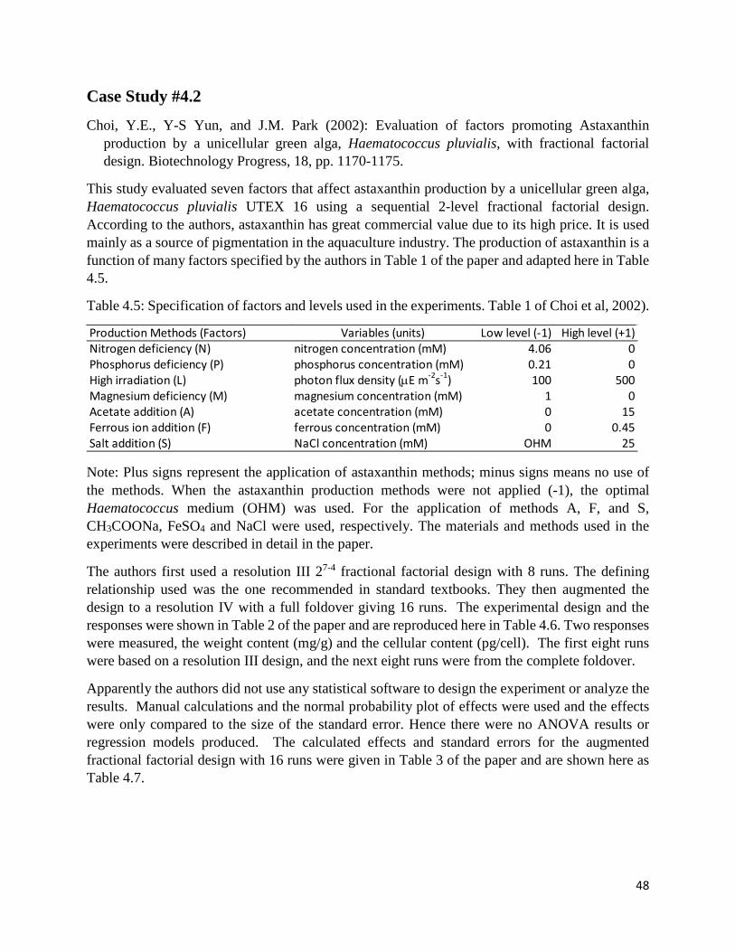
48
Case Study #4.2
Choi, Y.E., Y-S Yun, and J.M. Park (2002): Evaluation of factors promoting Astaxanthin production by a unicellular green alga, Haematococcus pluvialis, with fractional factorial design. Biotechnology Progress, 18, pp. 1170-1175.
This study evaluated seven factors that affect astaxanthin production by a unicellular green alga, Haematococcus pluvialis UTEX 16 using a sequential 2-level fractional factorial design. According to the authors, astaxanthin has great commercial value due to its high price. It is used mainly as a source of pigmentation in the aquaculture industry. The production of astaxanthin is a function of many factors specified by the authors in Table 1 of the paper and adapted here in Table 4.5.
Table 4.5: Specification of factors and levels used in the experiments. Table 1 of Choi et al, 2002).
Note: Plus signs represent the application of astaxanthin methods; minus signs means no use of the methods. When the astaxanthin production methods were not applied (-1), the optimal Haematococcus medium (OHM) was used. For the application of methods A, F, and S, CH3COONa, FeSO4 and NaCl were used, respectively. The materials and methods used in the experiments were described in detail in the paper.
The authors first used a resolution III 27-4 fractional factorial design with 8 runs. The defining relationship used was the one recommended in standard textbooks. They then augmented the design to a resolution IV with a full foldover giving 16 runs. The experimental design and the responses were shown in Table 2 of the paper and are reproduced here in Table 4.6. Two responses were measured, the weight content (mg/g) and the cellular content (pg/cell). The first eight runs were based on a resolution III design, and the next eight runs were from the complete foldover.
Apparently the authors did not use any statistical software to design the experiment or analyze the results. Manual calculations and the normal probability plot of effects were used and the effects were only compared to the size of the standard error. Hence there were no ANOVA results or regression models produced. The calculated effects and standard errors for the augmented fractional factorial design with 16 runs were given in Table 3 of the paper and are shown here as Table 4.7.
Production Methods (Factors) Variables (units) Low level (-1) High level (+1)Nitrogen deficiency (N) nitrogen concentration (mM) 4.06 0Phosphorus deficiency (P) phosphorus concentration (mM) 0.21 0High irradiation (L) photon flux density (µE m-2s-1) 100 500Magnesium deficiency (M) magnesium concentration (mM) 1 0Acetate addition (A) acetate concentration (mM) 0 15Ferrous ion addition (F) ferrous concentration (mM) 0 0.45Salt addition (S) NaCl concentration (mM) OHM 25
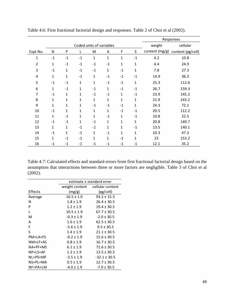
49
Table 4.6: First fractional factorial design and responses. Table 2 of Choi et al (2002).
Table 4.7: Calculated effects and standard errors from first fractional factorial design based on the assumption that interactions between three or more factors are negligible. Table 3 of Choi et al (2002).
weight cellularExpt No. N P L M A F S content (mg/g) content (pg/cell)
1 -1 -1 -1 1 1 1 -1 4.2 10.82 1 -1 -1 -1 -1 1 1 4.4 24.93 -1 1 -1 -1 1 -1 1 7.8 27.34 1 1 -1 1 -1 -1 -1 14.9 36.35 -1 -1 1 1 -1 -1 1 25.3 112.66 1 -1 1 -1 1 -1 -1 26.7 159.37 -1 1 1 -1 -1 1 -1 23.9 145.28 1 1 1 1 1 1 1 21.9 243.29 1 1 1 -1 -1 -1 1 24.3 72.110 -1 1 1 1 1 -1 -1 20.5 112.211 1 -1 1 1 -1 1 -1 10.8 22.512 -1 -1 1 -1 1 1 1 20.8 149.713 1 1 -1 -1 1 1 -1 13.5 140.114 -1 1 -1 1 -1 1 1 10.3 47.315 1 -1 -1 1 1 -1 1 23 153.216 -1 -1 -1 -1 -1 -1 -1 12.1 35.2
ResponsesCoded units of variables
weight content cellular contentEffects (mg/g) (pg/cell)Average 16.5 ± 1.0 93.2 ± 15.3N 1.8 ± 1.9 26.4 ± 30.5P 1.2 ± 1.9 19.4 ± 30.5L 10.5 ± 1.9 67.7 ± 30.5M -0.3 ± 1.9 -2.0 ± 30.5A 1.6 ± 1.9 62.5 ± 30.5F -5.6 ± 1.9 9.5 ± 30.5S 1.4 ± 1.9 21.1 ± 30.5PM+LA+FS -0.2 ± 1.9 15.6 ± 30.5NM+LF+AS 0.8 ± 1.9 16.7 ± 30.5NA+PF+MS 6.1 ± 1.9 72.6 ± 30.5NP+LS+AF 1.2 ± 1.9 13.5 ± 30.5NL+PS+MF -3.5 ± 1.9 -32.1 ± 30.5NS+PL+MA 0.5 ± 1.9 12.7 ± 30.5NF+PA+LM -4.0 ± 1.9 -7.0 ± 30.5
estimate ± standard error

50
According to the authors, only positive effects on the responses are important. Hence, for the weight content, from Table 4.7, the effects L, and the aliased interaction term NA+PF+MF are deemed significant since their effect estimates are larger than the standard error. Other effects were deemed not significant or they contribute a negative amount. For the response cellular content, the effects L, A, and the same aliased interaction term NA+PF+AF, are significant as they contribute positively to that response. However, the NA+PF+AF effect could also be due to the interactions of P and F or A and F, besides N and A. The authors reasoned that the NA interaction was most likely to be responsible for the positive effect of the confounded interaction NA+PF+AF.
To confirm the author’s suspicion, these interactions had to be de-aliased. To achieve this, the authors performed a single-factor foldover on factor A. This means that A was no longer aliased with other factors and was also de-aliased from all interactions involving A.
The results of the new set of 8 experiments folding over on A alone was shown in Table 4 of the paper and are shown here as Table 4.8. The combined data from the first 8 runs of the first experiment (Table 4.6) and from Table 4.8 were reanalyzed. The estimated effects and standard errors were shown in Table 5 of the paper and are reproduced here as Table 4.9.
Table 4.8: Additional fractional factorial design and responses. Table 4 of Choi et al (2002).
weight cellularExpt No. N P L M A F S content (mg/g) content (pg/cell)
17 -1 -1 -1 1 -1 1 -1 13.9 129.518 1 -1 -1 -1 1 1 1 9.3 268.819 -1 1 -1 -1 -1 -1 1 22 127.420 1 1 -1 1 1 -1 -1 20.8 135.921 -1 -1 1 1 1 -1 1 24.3 112.322 1 -1 1 -1 -1 -1 -1 27.6 119.723 -1 1 1 -1 1 1 -1 10.2 221.724 1 1 1 1 -1 1 1 2.8 35.3
ResponsesCoded units of variables
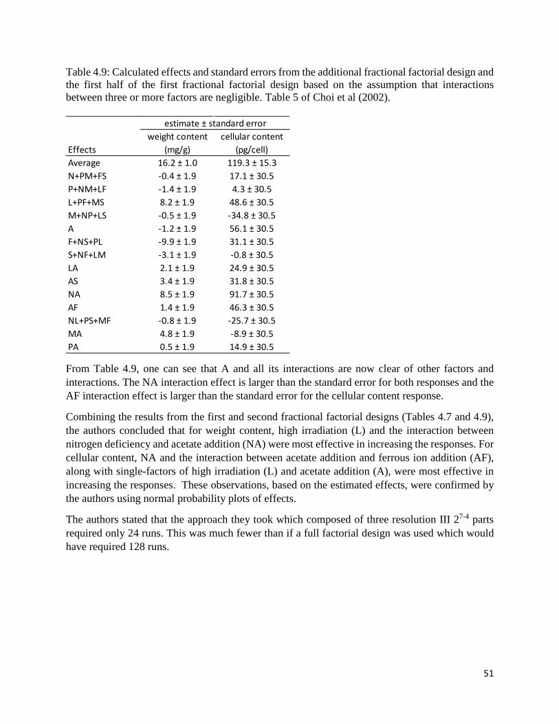
51
Table 4.9: Calculated effects and standard errors from the additional fractional factorial design and the first half of the first fractional factorial design based on the assumption that interactions between three or more factors are negligible. Table 5 of Choi et al (2002).
From Table 4.9, one can see that A and all its interactions are now clear of other factors and interactions. The NA interaction effect is larger than the standard error for both responses and the AF interaction effect is larger than the standard error for the cellular content response.
Combining the results from the first and second fractional factorial designs (Tables 4.7 and 4.9), the authors concluded that for weight content, high irradiation (L) and the interaction between nitrogen deficiency and acetate addition (NA) were most effective in increasing the responses. For cellular content, NA and the interaction between acetate addition and ferrous ion addition (AF), along with single-factors of high irradiation (L) and acetate addition (A), were most effective in increasing the responses. These observations, based on the estimated effects, were confirmed by the authors using normal probability plots of effects.
The authors stated that the approach they took which composed of three resolution III 27-4 parts required only 24 runs. This was much fewer than if a full factorial design was used which would have required 128 runs.
weight content cellular contentEffects (mg/g) (pg/cell)Average 16.2 ± 1.0 119.3 ± 15.3N+PM+FS -0.4 ± 1.9 17.1 ± 30.5P+NM+LF -1.4 ± 1.9 4.3 ± 30.5L+PF+MS 8.2 ± 1.9 48.6 ± 30.5M+NP+LS -0.5 ± 1.9 -34.8 ± 30.5A -1.2 ± 1.9 56.1 ± 30.5F+NS+PL -9.9 ± 1.9 31.1 ± 30.5S+NF+LM -3.1 ± 1.9 -0.8 ± 30.5LA 2.1 ± 1.9 24.9 ± 30.5AS 3.4 ± 1.9 31.8 ± 30.5NA 8.5 ± 1.9 91.7 ± 30.5AF 1.4 ± 1.9 46.3 ± 30.5NL+PS+MF -0.8 ± 1.9 -25.7 ± 30.5MA 4.8 ± 1.9 -8.9 ± 30.5PA 0.5 ± 1.9 14.9 ± 30.5
estimate ± standard error

52
Case Study #4.3
Farris, S. and Luciano Piergiovanni (2008): Effects of ingredients and process conditions on ‘Amaretti’ cookies characteristics. International Journal of Food Science and Technology, 43, pp. 1395-1403.
This study was concerned with the use of fractional factorial design on the factors that determine the quality and taste of the well-known Italian ‘Amaretti’ cookies during their shelf life. The characteristics studied included: hardness, moisture content, water activity, and colour of the cookies. The authors considered five controllable factors in their experiment and decided to study these factors using a half fraction of a 2-level factorial design i.e. a 25-1 design. The factors and levels used were given in Table 2 of the paper and are reproduced here as Table 4.10. For this experiment, the authors made some modifications to the original recipe by adding fibre and using fructose/saccharose (F/S) mixture instead of only saccharose. The level used in the original recipe was also shown in the table.
Table 4.10: Factors and their levels for both the 25-1 design and the original recipe. Table 2 of Farris et al (2008).
Four responses were measured in the experiment: Y1, Hardness (N-mm) – measured using a food texture analyzer; Y2, Moisture content (% H2O) – measured using Gravimetric analysis; Y3, Water activity – measured with an electronic hygrometer; and Y4, Colour – measured using an observer reflection colorimeter. These were described in the paper.
The authors chose a resolution V 25-1 design that required 16 runs. Five center points were added to measure pure error giving a total of 21 experiments. This design would allow all main effects and two-factor interactions to be estimated without bias. The experimental design and results were shown in Table 3 of the paper and are reproduced here as Table 4.11.
The authors used MODDE Version 8 software package by UMETRICS AB, Umea, Sweden for the evaluation of the raw data and regression analysis using the least squares method. A two-factor interaction model was fitted to each of the responses and only regression coefficients significant at the 5% level were selected for developing the final regression models.
The estimated coefficients of the fitted equations for the different responses were shown in Table 4 of the paper and are reproduced here as Table 4.12.
Variable Unit Coded Uncoded -1 0 +1 Original recipeFibre g X1 Fib 20 25 30 NoneF/S g/g X2 F/S 0.1 0.24 0.38 Only saccharose (650)Egg white g X3 Egg 250 257.5 265 255Temperature °C X4 Temp. 165 180 195 200Time Min X5 Time 18 20 22 20
Symbol Levels
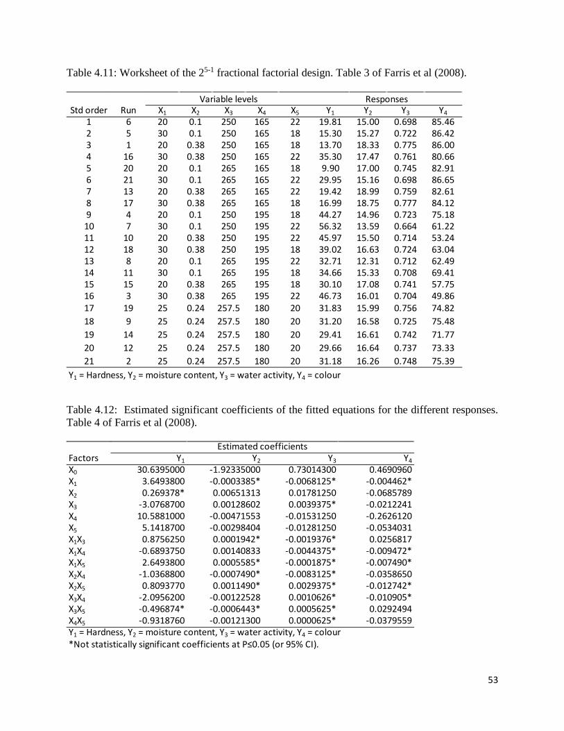
53
Table 4.11: Worksheet of the 25-1 fractional factorial design. Table 3 of Farris et al (2008).
Table 4.12: Estimated significant coefficients of the fitted equations for the different responses. Table 4 of Farris et al (2008).
Std order Run X1 X2 X3 X4 X5 Y1 Y2 Y3 Y41 6 20 0.1 250 165 22 19.81 15.00 0.698 85.462 5 30 0.1 250 165 18 15.30 15.27 0.722 86.423 1 20 0.38 250 165 18 13.70 18.33 0.775 86.004 16 30 0.38 250 165 22 35.30 17.47 0.761 80.665 20 20 0.1 265 165 18 9.90 17.00 0.745 82.916 21 30 0.1 265 165 22 29.95 15.16 0.698 86.657 13 20 0.38 265 165 22 19.42 18.99 0.759 82.618 17 30 0.38 265 165 18 16.99 18.75 0.777 84.129 4 20 0.1 250 195 18 44.27 14.96 0.723 75.1810 7 30 0.1 250 195 22 56.32 13.59 0.664 61.2211 10 20 0.38 250 195 22 45.97 15.50 0.714 53.2412 18 30 0.38 250 195 18 39.02 16.63 0.724 63.0413 8 20 0.1 265 195 22 32.71 12.31 0.712 62.4914 11 30 0.1 265 195 18 34.66 15.33 0.708 69.4115 15 20 0.38 265 195 18 30.10 17.08 0.741 57.7516 3 30 0.38 265 195 22 46.73 16.01 0.704 49.8617 19 25 0.24 257.5 180 20 31.83 15.99 0.756 74.8218 9 25 0.24 257.5 180 20 31.20 16.58 0.725 75.4819 14 25 0.24 257.5 180 20 29.41 16.61 0.742 71.7720 12 25 0.24 257.5 180 20 29.66 16.64 0.737 73.3321 2 25 0.24 257.5 180 20 31.18 16.26 0.748 75.39
Y1 = Hardness, Y2 = moisture content, Y3 = water activity, Y4 = colour
Variable levels Responses
Factors Y1 Y2 Y3 Y4X0 30.6395000 -1.92335000 0.73014300 0.4690960X1 3.6493800 -0.0003385* -0.0068125* -0.004462*X2 0.269378* 0.00651313 0.01781250 -0.0685789X3 -3.0768700 0.00128602 0.0039375* -0.0212241X4 10.5881000 -0.00471553 -0.01531250 -0.2626120X5 5.1418700 -0.00298404 -0.01281250 -0.0534031X1X3 0.8756250 0.0001942* -0.0019376* 0.0256817X1X4 -0.6893750 0.00140833 -0.0044375* -0.009472*X1X5 2.6493800 0.0005585* -0.0001875* -0.007490*X2X4 -1.0368800 -0.0007490* -0.0083125* -0.0358650X2X5 0.8093770 0.0011490* 0.0029375* -0.012742*X3X4 -2.0956200 -0.00122528 0.0010626* -0.010905*X3X5 -0.496874* -0.0006443* 0.0005625* 0.0292494X4X5 -0.9318760 -0.00121300 0.0000625* -0.0379559Y1 = Hardness, Y2 = moisture content, Y3 = water activity, Y4 = colour*Not statistically significant coefficients at P≤0.05 (or 95% CI).
Estimated coefficients

54
The interaction terms X1X2 and X2X3 were removed beforehand because they were deemed statistically insignificant at the 5% level. However, many of the coefficients were also identified as statistically insignificant in addition to the two removed in Table 4.12. Furthermore, one can see that the coefficients given for Y2 and Y4 seem to be clearly wrong by orders of magnitude. The coefficients for Y1 and Y3, however, are correct.
The goodness-of-fit statistics for the four responses after model refinement (based on the terms in Table 4.12) were given in Table 5 of the paper, and are shown here as Table 4.13.
Table 4.13: Summary list for the four model parameters after model refinement. Table 5 of Farris et al (2008).
The statistic Q2, called the power of prediction (an uncommon term), is likely equivalent to the more commonly used term, the predicted R2. The term model validity and reproducibility were not defined in the paper.
The ANOVA results for Y1, Y2, and Y4 are shown in Table 6 of the paper. No suitable model was found for Y3, the water activity (negative Q2). These results used all terms except the two two-factor interactions X1X2 and X2X3. The ANOVA results are reproduced here in Table 4.14.
Table 4.14: ANOVA table for the response of hardness, moisture content and colour. Adapted from Table 6 of Farris et al (2008).
A closer look at the ANOVA results showed that the results for Y2 and Y4 are also incorrect by an order of magnitude. It seems that the authors may have used the wrong data in their analysis. In addition, no test for curvature was done.
Response R2 R2adj. Q2 Model validity ReproducibilityHardness 0.977 0.991 0.930 0.794 0.992Moisture content 0.980 0.943 0.584 0.558 0.968Water activity 0.886 0.675 -1.023 0.529 0.828Colour 0.995 0.986 0.965 0.941 0.980
Parameter
Source of variation DF SS MS F SS MS F SS MS FTotal 21 22553.1 1073.96 77.699 3.699 5.934 0.282Constant 1 19714.4 19714.4 77.684 77.684 4.621 4.621Tot. corrected 20 2838.71 141.936 0.001 6.82E-05 1.312 0.065Regression 13 2830.45 217.727 184.52 0.001 0.0001 26.83 1.306 0.100 109.78Residual 7 8.259 1.179 2.68E-05 3.83E-06 0.006 0.0009Lack of fit (model error) 3 3.766 1.255 1.11 1.82E-05 6.07E-06 2.81 0.001 0.0004 0.35Pure error (replicate error) 4 4.493 1.123 8.63E-06 2.15E-06 0.005 0.001
F0.95; 13;7 = 3.55 R2 = 0.997 R2 = 0.980 R2 = 0.995
F0.95; 3;4 = 6.59
Y1 (Hardness) Y2 (moisture content) Y4 (colour)

55
The final prediction models for the three responses suggested by the authors were:
Hardness (Y1) = 30.64 + 3.65 X1 - 3.08 X3 + 10.59 X4 + 5.14 X5 + 0.88 X1X3 – 0.69 X1X4 + 2.65 X1X5 – 1.04 X2X4 + 0.81X2X5 – 2.10 X3X4 – 0.93 X4X5
Moisture content (Y2) = -1.92 + 0.00651 X2 + 0.00129 X3 – 0.00471 X4 -0.00298 X5
+ 0.00141 X1X4 – 0.00122 X3X4 – 0.00121 X4X5
Colour (Y4) = 0.47 – 0.069 X2 – 0.021 X3 – 0.263 X4 - 0.053 X5 + 0.025 X1X3 – 0.035 X2X4
+ 0.029 X3X5 – 0.038 X4X5
No goodness-of-fit statistics were given for these reduced models. Also, it should be noted that the models given are not hierarchical and may not lead to the correct predictions. As mentioned earlier, all the coefficients for Y2 and Y4 are incorrect.
Case Study #4.4
Hajeeh, M. (2003): Estimating corrosion: a statistical approach. Materials and Design, 24, pp. 509-518.
This study used a fractional factorial design to investigate the factors that affect the corrosivity of seawater on aluminum-brass (Al-brass) and carbon steel (C-S) alloy pipes. The original plan was to investigate seven factors using a half-fraction of a two-level factorial design i.e. 27-1 design with 64 runs. However, the author found that since the corrosion rates for the two alloys were very different and the error variance for C-S alloy was larger than that of the Al-brass alloy, difficulties might arise in the interpretation of the estimated effects. Hence, the experiment was decomposed into two separate six-factor 26-1 designs instead of using alloy type as one of the factors. The six factors and levels used in the two designs were given in Table 1 of the paper and are reproduced here as Table 4.15.
Table 4.15: Variables of the experiments and their levels. Table 1 of Hajeeh (2003).
Variable Units Low level High level Temperature (T) °C 30 45 Oxygen (O2) Deaerated Aerated Urea (U) ppm 0 3.5 Inhibitor (I) ppm 0 50 Sulfide (S) ppm 0 2 Chloride (C ) ppm 19500 23000

56
The 26-1 design is a resolution VI design, where all main effects and two-factor interactions are not aliased with any other effects or interactions. However, three-factor interactions are aliased with other three-factor interactions. Although not mentioned in the paper, the defining relationships used for the Al-brass was I=ABCDEF, and for the C-S was I = -ABCDEF. The response measured for each experiment was the corrosion rate in mils per year (mpy). The experimental design and the corrosion rates for the Al-brass alloy and C-S alloy were shown in Tables 2 and 3 of the paper and are reproduced here as Tables 4.16 and 4.17.
Table 4.16: Experimental design and corrosion rates for Al-brass. Table 2 of Hajeeh (2003).
A (aerated): the environment is full of oxygen, D (deaerated): the environment does not contain any oxygen.
Temperature Oxygen Urea Sulfide Inhibitor Chloride Corrosion rate ReplicationExpt No. (°C) (ppm) (ppm) (ppm) (ppm) (ppm) (mpy)
1 30 D 0 0 0 19500 1.12 45 A 0 0 0 19500 0.9 0.73 45 D 3.5 0 0 19500 0.34 30 A 3.5 0 0 19500 0.6 0.95 45 D 0 2 0 19500 0.76 30 A 0 2 0 19500 1.17 30 D 3.5 2 0 19500 1.68 45 A 3.5 2 0 19500 1.6 1.19 45 D 0 0 50 19500 0.2
10 30 A 0 0 50 19500 1.411 30 D 3.5 0 50 19500 1.112 45 A 3.5 0 50 19500 0.2 0.213 30 D 0 2 50 19500 0.414 45 A 0 2 50 19500 0.915 45 D 3.5 2 50 19500 0.416 30 A 3.5 2 50 19500 0.517 45 D 0 0 0 23000 1.318 30 A 0 0 0 23000 0.7 0.719 30 D 3.5 0 0 23000 0.320 45 A 3.5 0 0 23000 1.321 30 D 0 2 0 23000 1.122 45 A 0 2 0 23000 1.123 45 D 3.5 2 0 23000 0.224 30 A 3.5 2 0 23000 1.0 1.625 30 D 0 0 50 23000 0.126 45 A 0 0 50 23000 0.127 45 D 3.5 0 50 23000 0.128 30 A 3.5 0 50 23000 0.629 45 D 0 2 50 23000 0.330 30 A 0 2 50 23000 0.631 30 D 3.5 2 50 23000 0.9 0.2432 45 A 3.5 2 50 23000 0.5
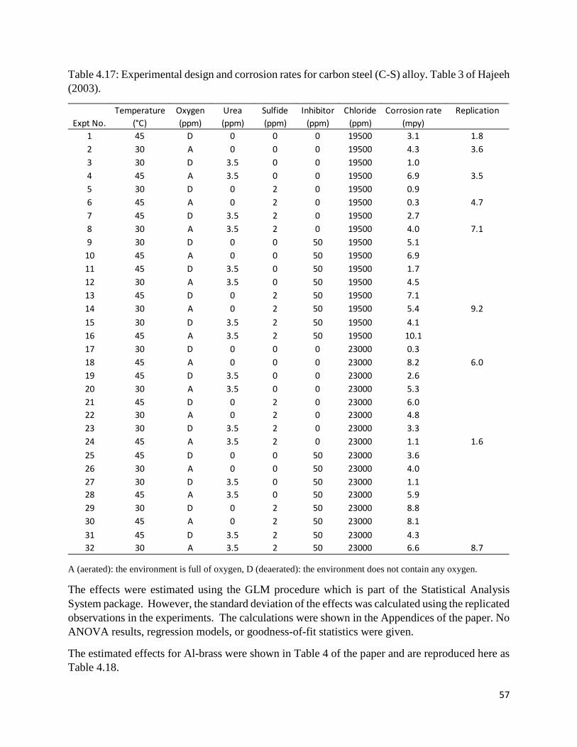
57
Table 4.17: Experimental design and corrosion rates for carbon steel (C-S) alloy. Table 3 of Hajeeh (2003).
A (aerated): the environment is full of oxygen, D (deaerated): the environment does not contain any oxygen.
The effects were estimated using the GLM procedure which is part of the Statistical Analysis System package. However, the standard deviation of the effects was calculated using the replicated observations in the experiments. The calculations were shown in the Appendices of the paper. No ANOVA results, regression models, or goodness-of-fit statistics were given.
The estimated effects for Al-brass were shown in Table 4 of the paper and are reproduced here as Table 4.18.
Temperature Oxygen Urea Sulfide Inhibitor Chloride Corrosion rate ReplicationExpt No. (°C) (ppm) (ppm) (ppm) (ppm) (ppm) (mpy)
1 45 D 0 0 0 19500 3.1 1.82 30 A 0 0 0 19500 4.3 3.63 30 D 3.5 0 0 19500 1.04 45 A 3.5 0 0 19500 6.9 3.55 30 D 0 2 0 19500 0.96 45 A 0 2 0 19500 0.3 4.77 45 D 3.5 2 0 19500 2.78 30 A 3.5 2 0 19500 4.0 7.19 30 D 0 0 50 19500 5.110 45 A 0 0 50 19500 6.911 45 D 3.5 0 50 19500 1.712 30 A 3.5 0 50 19500 4.513 45 D 0 2 50 19500 7.114 30 A 0 2 50 19500 5.4 9.215 30 D 3.5 2 50 19500 4.116 45 A 3.5 2 50 19500 10.117 30 D 0 0 0 23000 0.318 45 A 0 0 0 23000 8.2 6.019 45 D 3.5 0 0 23000 2.620 30 A 3.5 0 0 23000 5.321 45 D 0 2 0 23000 6.022 30 A 0 2 0 23000 4.823 30 D 3.5 2 0 23000 3.324 45 A 3.5 2 0 23000 1.1 1.625 45 D 0 0 50 23000 3.626 30 A 0 0 50 23000 4.027 30 D 3.5 0 50 23000 1.128 45 A 3.5 0 50 23000 5.929 30 D 0 2 50 23000 8.830 45 A 0 2 50 23000 8.131 45 D 3.5 2 50 23000 4.332 30 A 3.5 2 50 23000 6.6 8.7

58
Table 4.18: Estimates of various effects and interactions for Al-brass alloy. (Table 4 of Hajeeh (2003).
For the Al-brass data, the author calculated the standard deviation of effects to be 0.1027 and the 95% confidence interval as ±0.243. Hence any absolute value of estimated effect that was greater than 0.243 were considered statistically significant at the 5% level. The author identified the following effects to be statistically significant at the 5% level:
a. Inhibitor b. Oxygen × urea × inhibitor + temperature × sulfide × chloride c. Temperature × inhibitor × sulfide + urea × inhibitor × chloride d. Temperature × oxygen × urea + sulfide × inhibitor × chloride e. Temperature × inhibitor × chloride + oxygen × urea × sulfide
The author also identified those effects that were statistically significant at the 10% and 20% levels in the paper.
The estimate for the temperature × inhibitor × sulfide + urea × inhibitor × chloride interaction is missing from Table 4.18. In any case, the three-factor interaction of temperature × inhibitor × sulfide should be aliased with oxygen × urea × chloride and not urea × inhibitor × chloride. There are actually several other typographical errors or wrong estimates in Table 4.18.
For the carbon-steel alloy, the effect estimates were given in Table 6 of the paper and are reproduced here as Table 4.19. The author did not explain why the aliased terms were not shown, as in Table 4.18.
Effect/Interaction Estimated effect Effect/Interaction Estimated effectMean 0.7250 T X O2 X U + S X I X C 0.2750Temperature -0.1875 T X O2 X S + U X I X C 0.2125Oxygen 0.1875 T X O2 X I + U X S X C -0.1875Urea 0.0500 T X U X S + O2 X I X C -0.0750Sulfide 0.1625 T X U X I + O2 X U X S -0.0500Inhibitor -0.4125 T X I X C + O2 X U X S 0.2875T X O2 0.2000 O2 X U X S + T X I X C -0.0750T X U 0.0625 O2 X U X I + T X S X C -0.3250T X S 0.0000 O2 X I X C + T X U X S -0.0625T X I -0.1750 U X S X I + T X O2 X C -0.1250O2 X U -0.0125 I X C -0.0625O2 X S 0.0250 S X C -0.0125O2 X I -0.0250 U X C 0.0000U X S 0.1125 O2 X C 0.0125U X I 0.0875 T X C 0.1375S X I -0.0750 Chloride -0.1750

59
Table 4.19: Estimates of main effects and interactions for carbon-steel alloy. Table 6 of Hajeeh (2003).
The standard deviation of effects was obtained using the replicated observations and was calculated to be 0.663. The 95% confidence interval was ±1.523. Based on this interval, the author identified the following effects as significant at the 5% level:
a. Oxygen b. Temperature c. Sulfide.
Other effects that were statistically significant at the 20% level were identified. However, the estimates given by the author are highly suspect as the mean was estimated incorrectly. It should be 4.44 and not 9.78. All other estimates seem to be incorrect as well.
The author concluded that, for the aluminum-brass alloy, the inhibitor contributed significantly to decreasing corrosion rates, and there were also various significant three-factor interactions. For carbon-steel alloy, only oxygen, temperature, and sulfide were most significant, followed by a few two-factor interactions that were moderately significant. However, given the frequency of errors in the paper, these conclusions may not be entirely correct.
There was no mention of ANOVA assumption checks or whether there were any follow-up experiments to de-alias the three-factor interactions.
Effect/Interaction Estimated effect Effect/Interaction Estimated effectMean 9.7800 T X O2 X U -0.0063Temperature 1.8440 T X O2 X S 0.2440Oxygen 2.0990 T X O2 X I 0.5810Urea -0.8310 T X U X S -0.0063Sulfide 1.7190 T X U X I 0.7810Inhibitor 1.1310 T X S X I -0.0188T X O2 1.0300 O2 X U X S 0.3188T X U -0.3690 O2 X U X I 1.0810T X S 0.1810 O2 X S X I 0.1310T X I -0.8310 U X S X I 0.2810O2 X U 0.9310 I X C 0.5810O2 X S -0.9220 S X C -0.5810O2 X I -0.8560 U X C 0.0686U X S -0.0188 O2 X C 0.2688U X I -0.5063 T X C 0.3440S X I 0.9940 Chloride 0.2690

60
Case Study #4.5
Kazemi-Beydokhti, A., Hamed Azizi Namaghi, and Saeed Zeinali Heris (2013): Identification of the key variables on thermal conductivity of CuO nanofluid by a fractional factorial design approach. Numerical Heat Transfer, Part B, 64, pp. 480-495.
This study investigated seven parameters that are responsible for change in the thermal conductivity of nanofluids containing copper oxide nano particles. The authors started by using a resolution III 27-4 fractional factorial design with eight runs and three center points and then augmented with a full-foldover design of another eight runs and three center points. The total number of runs was 22. The factors and levels used in the fractional factorial experiments were given in Table 1 of the paper and are reproduced here as Table 4.20.
Table 4.20: Factors and levels for full-foldover fractional factorial design. Table 1 of Kazemi-Beydokhti et al (2013).
The initial fractional factorial design was a 1/16th fraction of resolution III. This means that each effect will be aliased with 15 other effects. More importantly, the main effects will be aliased with two-factor interactions. The defining relationship used for the design was recommended in standard textbooks and Design-Expert version 8.0.0.6 software which was used by the authors for experimental design and analysis of the data.
The details of the experiment and how thermal conductivity measurements were taken were explained in the paper. The response used was the ratio of the thermal conductivity of the nanofluids Knf to that of the base fluid, Kf; that is, Knf/Kf.
The initial experimental design and the results were shown in Table 2 of the paper and are reproduced here as Table 4.21.
Factor Unit -1 (Low) 0 (Center point) +1 (High)[A] Temperature C 25 35 45[B] Particle volume fraction %vol 2 3 4[C] APPS nm 30 40 50[D] pH of nanofluid 2 7 12[E] Elapsed time h 0 5 10[F] Sonication time h 1 2 3[G] Density of nanoparticles kg/m3 2000 4000 6000
Level
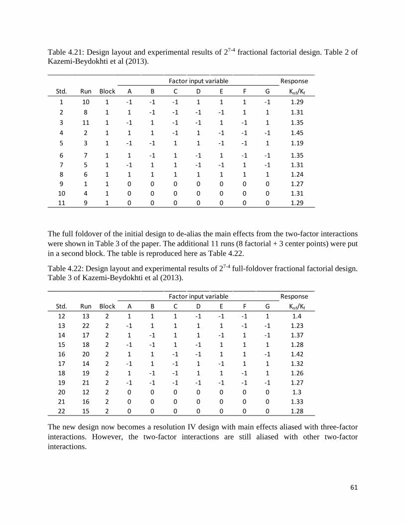
61
Table 4.21: Design layout and experimental results of 27-4 fractional factorial design. Table 2 of Kazemi-Beydokhti et al (2013).
The full foldover of the initial design to de-alias the main effects from the two-factor interactions were shown in Table 3 of the paper. The additional 11 runs (8 factorial + 3 center points) were put in a second block. The table is reproduced here as Table 4.22.
Table 4.22: Design layout and experimental results of 27-4 full-foldover fractional factorial design. Table 3 of Kazemi-Beydokhti et al (2013).
The new design now becomes a resolution IV design with main effects aliased with three-factor interactions. However, the two-factor interactions are still aliased with other two-factor interactions.
ResponseStd. Run Block A B C D E F G Knf/Kf
1 10 1 -1 -1 -1 1 1 1 -1 1.292 8 1 1 -1 -1 -1 -1 1 1 1.313 11 1 -1 1 -1 -1 1 -1 1 1.354 2 1 1 1 -1 1 -1 -1 -1 1.455 3 1 -1 -1 1 1 -1 -1 1 1.19
6 7 1 1 -1 1 -1 1 -1 -1 1.357 5 1 -1 1 1 -1 -1 1 -1 1.318 6 1 1 1 1 1 1 1 1 1.249 1 1 0 0 0 0 0 0 0 1.2710 4 1 0 0 0 0 0 0 0 1.3111 9 1 0 0 0 0 0 0 0 1.29
Factor input variable
ResponseStd. Run Block A B C D E F G Knf/Kf
12 13 2 1 1 1 -1 -1 -1 1 1.413 22 2 -1 1 1 1 1 -1 -1 1.2314 17 2 1 -1 1 1 -1 1 -1 1.3715 18 2 -1 -1 1 -1 1 1 1 1.2816 20 2 1 1 -1 -1 1 1 -1 1.4217 14 2 -1 1 -1 1 -1 1 1 1.3218 19 2 1 -1 -1 1 1 -1 1 1.2619 21 2 -1 -1 -1 -1 -1 -1 -1 1.2720 12 2 0 0 0 0 0 0 0 1.321 16 2 0 0 0 0 0 0 0 1.3322 15 2 0 0 0 0 0 0 0 1.28
Factor input variable
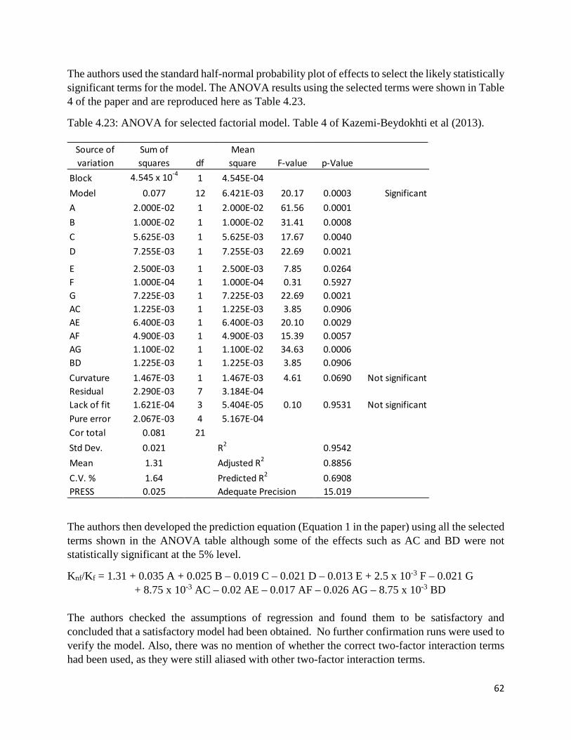
62
The authors used the standard half-normal probability plot of effects to select the likely statistically significant terms for the model. The ANOVA results using the selected terms were shown in Table 4 of the paper and are reproduced here as Table 4.23.
Table 4.23: ANOVA for selected factorial model. Table 4 of Kazemi-Beydokhti et al (2013).
The authors then developed the prediction equation (Equation 1 in the paper) using all the selected terms shown in the ANOVA table although some of the effects such as AC and BD were not statistically significant at the 5% level.
Knf/Kf = 1.31 + 0.035 A + 0.025 B – 0.019 C – 0.021 D – 0.013 E + 2.5 x 10⁻³ F – 0.021 G + 8.75 x 10⁻³ AC – 0.02 AE – 0.017 AF – 0.026 AG – 8.75 x 10⁻³ BD The authors checked the assumptions of regression and found them to be satisfactory and concluded that a satisfactory model had been obtained. No further confirmation runs were used to verify the model. Also, there was no mention of whether the correct two-factor interaction terms had been used, as they were still aliased with other two-factor interaction terms.
Source of variation
Sum of squares df
Mean square F-value p-Value
Block 4.545 x 10⁻⁴ 1 4.545E-04Model 0.077 12 6.421E-03 20.17 0.0003 SignificantA 2.000E-02 1 2.000E-02 61.56 0.0001B 1.000E-02 1 1.000E-02 31.41 0.0008C 5.625E-03 1 5.625E-03 17.67 0.0040D 7.255E-03 1 7.255E-03 22.69 0.0021
E 2.500E-03 1 2.500E-03 7.85 0.0264F 1.000E-04 1 1.000E-04 0.31 0.5927G 7.225E-03 1 7.225E-03 22.69 0.0021AC 1.225E-03 1 1.225E-03 3.85 0.0906AE 6.400E-03 1 6.400E-03 20.10 0.0029AF 4.900E-03 1 4.900E-03 15.39 0.0057AG 1.100E-02 1 1.100E-02 34.63 0.0006BD 1.225E-03 1 1.225E-03 3.85 0.0906Curvature 1.467E-03 1 1.467E-03 4.61 0.0690 Not significantResidual 2.290E-03 7 3.184E-04Lack of fit 1.621E-04 3 5.404E-05 0.10 0.9531 Not significantPure error 2.067E-03 4 5.167E-04Cor total 0.081 21Std Dev. 0.021 R2 0.9542Mean 1.31 Adjusted R2 0.8856C.V. % 1.64 Predicted R2 0.6908PRESS 0.025 Adequate Precision 15.019

63
Case Study #4.6
Levingstone, T. J., Malika Ardhaoui, Khaled Benyyounis, Lisa Looney, and Joseph T. Stokes (2015): Plasma sprayed hydroxyapatite coatings: Understanding process relationships using design of experiments analysis. Surface and Coatings Technology, 283, pp. 29-36.
This study used a fractional factorial (25-2) design to investigate the simultaneous effects of key plasma spray process parameters on hydroxyapatite coatings for biomedical applications. Hydroxyapatite is ceramic which has a similar mineral component to bone. Hence it has many applications particularly in the field of dentistry and orthopaedics. The authors considered the effects of five plasma spray process parameters on the roughness, crystallinity, and purity of hydroxyapatite coatings. The parameters and levels used in the fractional factorial design were shown in Table 1 of the paper and are reproduced here as Table 4.24.
Table 4.24: Parameter ranges selected for the screening experiment. Table 1 of Levingstone et al (2015).
Parameter Unit Low level (-1) High level (+1) A - Current A 450 750 B - Gas flow rate slpm/scfh 33/70 61.4/130 C - Powder feed rate g/min 10 20 D - Spray distance mm 80 120 E - Carrier gas flow rate slpm/scfh 4.7/10 9.4/20
The gas flow rates were given in two different units. It seems that that authors used the second unit which is scfh or standard cubic feet per hour.
Three responses were measured for each run combination. These were roughness (µm), crystallinity (%), and purity (%). The techniques and equipment used were described in the paper.
The experimental design and the results obtained were shown in Tables 2 and 3 in the paper and are combined here as Table 4.25. The defining relationship used for the resolution III fractional factorial (25-2) design was not mentioned in the paper but it can be deduced that it was the default used in Design-Expert 7.0 software package. Three centre points were added giving 11 runs for this screening experiment.
According to the authors, the coating from experiment N1 was very thin and measurements of crystallinity and purity could not be obtained. Furthermore, the roughness values were very low. Hence the results for N1 were not used for further analysis. Only experiments N2-N11 were used.

64
Table 4.25: Plasma spray screening experimental design and responses. Combined results from Tables 2 and 3 of Levingstone et al (2015).
The authors fitted only a main effects model to each of the responses using a backward elimination procedure in Design-Expert 7.0. A p-value of 0.01 was used. The regression models obtained for each response in coded and actual units were given in Table 4 of the paper and are reproduced below.
Coded: Roughness = 9.45 + 1.4 A – 1.17 B + 1.10 C
Actual: Roughness = 4.257 + 9.70417 E-003 X Current – 0.039146 X Gas flow rate + 0.21912 X Powder feed rate.
Coded: Crystallinity = 71.83 + 6.2 A – 5.16 D – 6.14 E Actual: Crystallinity = 91.25062 + 0.041329 X Current – 0.25797 X Spray distance
-1.22939 X Carrier gas flow rate.
Coded: Purity = 97.93 – 0.46 C – 0.34 D – 0.59 E Actual: Purity = 102.8 – 0.09125 X Power feed rate – 0.017187 X Spray distance
-0.11875 X Carrier gas flow rate
The goodness-of-fit for each of the above models were shown in Table 5 of the paper and reproduced here as Table 4.26. The authors did not mention if assumptions of regression were checked.
Exp. NameCurrent -
AGas flow rate -
BPowder feed
rate - CSpray
distance - DCarrier gas
flow rate - E Roughness Crystallinity Purity(A) (scfh) (g/min) (mm) (scfh) (µm) (%) (%)
N1 450 70 10 120 20 4.1N2 750 70 10 80 10 10.55 87.6 99.4N3 450 130 10 80 20 6.15 65.2 97.8N4 750 130 10 120 10 8.65 81.3 98.9N5 450 70 20 120 10 10.48 65.2 97.6N6 750 70 20 80 20 13.4 77.4 97.7N7 450 130 20 80 10 7.28 77.8 98.2N8 750 130 20 120 20 11.03 65.8 96.4N9 600 100 15 100 15 10.65 79.9 97.4
N10 600 100 15 100 15 9.48 54.9 95.5N11 600 100 15 100 15 10.6 76.1 97.2
Variables Responses

65
Table 4.26: Statistical measures of equation adequacy. Table 5 of Levingstone et al (2015).
The statistical measures given in Table 4.26 show that the fitted main effects model seems to provide a good fit to the responses obtained. Hence the authors concluded that the predictive equations developed were satisfactory and provided a better understanding of the effect of plasma spray properties on the roughness, crystallinity, and purity of hydroxyapatite coatings.
However, since the experimental design was a resolution IV design, two-factor interactions were all aliased with other two-factor interactions. It is likely that there are other statistically significant two-factor interactions not included in the models. To this end, follow up experiments were alluded to by the authors.
Case Study #4.7
Lucas, Y., Antonio Domingues, Driss Driochi, and Sylvie Treuillet (2006): Design of experiments for performance evaluation and parameter tuning of a road image processing chain. EURASIP Journal on Applied Signal Processing, Article ID 48012, pp. 1-10.
This study investigated the use of design of experiments techniques in tuning a full image processing chain (IPC) which is not a straightforward task. This was applied to a road image processing chain dedicated to road obstacles detection which has eight reconfigurable parameters and can be modified at any time. These parameters were shown in Table 1 of the paper and are reproduced here as Table 4.26. The details of the IPC and these parameters were described in the paper.
Table 4.26: Factors and levels used in the experiment. (Adapted from Table 1 of Lucas et al (2006).
Factor Parameter Low Level High level X1 Canny-Deriche filter 0.5 1 X2 Image amplification 33 63 X3 Edge low threshold 5 15 X4 Edge high threshold 15 30 X5 Contour closing 26 30 X6 Polygonal approximation 5 6 X7 Little chain threshold 5 10 X8 Slope threshold 1 3
Statistical measure Roughness Crystallinity PurityR2 0.95 0.96 0.91Adjusted R2 0.92 0.92 0.85Predicted R2 0.82 0.81 0.56Adequate precision 17.776 14.902 10.44

66
The authors proposed a quality evaluation criterion called the covering rate (r%) as the response from various combinations of the parameters. The exact definition of r was given in the paper. Basically, the criterion r is dependent on the image content. A high score means that most of the image has been extracted, hence it was expressed as a percentage.
The authors first considered a two-level fractional factorial (2k-p) design with 16 trials, then a Rechtschaffer [1] design with 37 trials, and finally a three-level factorial design (33) with 27 trials. Since the Rechtschaffer design is outside the scope of this Chapter and the three-level design was not analyzed by the authors, only the two-level fractional factorial design is presented here.
The experimental design and response r (%) were shown in Table 2 of the paper and reproduced here as Table 4.27.
Table 4.27: Experiment matrix-fractional factorial 28-4 design*: averaged outputs. Table 2 of Lucas et al (2006).
*Table 2 of Lucas et al (2006) incorrectly stated that it is a 28-3 design.
To obtain the response, according to the authors, each run combination was compared to 180 input images selected from a video sequence of over 30,000 city and motorway frames. Note that the experimental design was incorrectly labelled as a 28-3 design. A 28-3 design would need 32 runs not 16. In fact, a 28-3 does not exist. The smallest number of runs possible is a 28-4 design. The authors did not indicate what design generators were used to obtain the 28-4 design with 16 runs. By examining the run combinations, the authors have used the following design generators: X5 = X2X3X4, X6 = X1X3X4, X7 = X1X2X3, X8=X1X2X4. The design was a resolution IV design.
Trail X1 X2 X3 X4 X5 X6 X7 X8 r (%)1 -1 -1 -1 -1 -1 -1 -1 -1 35.5352 -1 -1 -1 1 1 1 -1 1 40.3103 -1 -1 1 -1 1 1 1 -1 27.8594 -1 -1 1 1 -1 -1 1 1 42.4365 -1 1 -1 -1 1 -1 1 1 47.3286 -1 1 -1 1 -1 1 1 -1 30.2847 -1 1 1 -1 -1 1 -1 1 44.0348 -1 1 1 1 1 -1 -1 -1 37.7439 1 -1 -1 -1 -1 1 1 1 46.517
10 1 -1 -1 1 1 -1 1 -1 40.46911 1 -1 1 -1 1 -1 -1 1 50.68012 1 -1 1 1 -1 1 -1 -1 33.46413 1 1 -1 -1 1 1 -1 -1 35.16914 1 1 -1 1 -1 -1 -1 1 49.25515 1 1 1 -1 -1 -1 1 -1 39.71516 1 1 1 1 1 1 1 1 44.842
67
Fitting a main effects model to the experimental data, the authors obtained the following prediction equation in actual units (Equation 4 in the paper):
Y = 51.1965 + 8.65 X1 – 4.08 X6 + 4.31 X8,
where, X1, X2, X3 are previously defined in Table 4.26.
The significance level used was not mentioned. They chose the 3 factor model that gave the second lowest Mallow’s Cp (3.48) and second highest R2 (0.938), instead of the four factor model which gave the lowest Cp (3,36) and highest R2 (0.950), arguing that the additional factor provided only a marginal improvement to the fit.
The authors also compared the tuning results and computing cost of eight different tuning methods of which three were based on design of experiments. The fractional factorial design required the least number of runs, and optimal tuning using only the three identified significant parameters gave the best results. One of the reasons given for the efficiency of the experimental design approach was that the IPC is globally optimized.
[1] Rechtschaffer, R. L. (1967): Saturated fractions of 2n and 3n factorial designs. Technometrics, Vol. 9, pp. 569-575.
Case Study #4.8
Ramakrishna, D. M., T. Viraraghavan, and Yee-Chung Jin (2006): Iron oxide coated sand for arsenic removal: investigation of coating parameters using factorial design approach. Practice Periodical of Hazardous, Toxic, and Radioactive Waste Management, Vol. 10, No. 4, pp. 198-206.
This study investigated seven factors that affect the iron oxide-coated sand filtration process for removing arsenic from drinking water. The seven factors were: coating pH (pHc), temperature (T), iron concentration (Fe), number of coatings (N), aging (age), pH of the solution (pHs), and mass of the adsorbent (M). The responses measured were the percentage removal of arsenic (V) and arsenic (III). The advantages of using iron oxide-coated sand was explained in detail in the paper. The experiments were carried out at room temperature in a laboratory as explained by the authors.
Minitab 14 software was used for the design and analysis of the experiment. The authors used a resolution III seven factor two-level fractional factorial (27-4) design with two replications followed up by a full-foldover of this design, making it into a resolution IV design. 32 run combinations were used, in total. The factors and levels used were given in Table 3 of the paper and are reproduced here as Table 4.28.

68
Table 4.28: Design parameters and their levels. Table 3 of Ramakrishna et al (2006).
Factor Code Low level High level pHc A 2.0 12.0
T B 110 °C 800 °C Fe C 0.1 M 2 M N D 1 2
Age E 4 h 12 days pHs F 5 9 M G 0.1 g 1 g
The first set of experiments which consisted of 16 runs (2 replicates of a 27-4 design) were shown in Table 4 of the paper and are reproduced here as Table 4.29 with corrections. In Table 4 of the paper, the responses were interchanged. That is, As(V) was listed as As(III), and As (III) was listed as As(V). Table 4.29: Fractional factorial design used in studies on removal of As(V) and As(III): Set I. Table 4 of Ramakrishna et al (2006).
*Note: As(V) was incorrectly listed as As(III), and As(III) was incorrectly listed as As(V) in Table 4 of Ramakrishna et al (2006). The first set of experiments were not statistically analyzed because all the main effects were confounded or aliased with two-factor interaction terms. To de-alias the main effects from the two-factor interactions, a full-foldover was conducted with another 16 runs. This procedure converted the design into a resolution IV design. Now the main effects were aliased with three-
pHc T Fe N Age pHs MNumber A B C D=AB E=AC F=BC G=ABC As(V)* AS(III)*
1 -1 -1 1 1 -1 -1 1 90.60 58.502 1 1 1 1 1 1 1 4.04 19.803 -1 1 -1 -1 1 -1 1 51.70 52.104 1 -1 -1 -1 -1 1 1 59.60 20.405 -1 1 -1 -1 1 -1 1 60.80 44.806 1 -1 -1 -1 -1 1 1 57.70 22.907 1 1 -1 1 -1 -1 -1 49.50 12.308 -1 1 1 -1 -1 1 -1 8.00 1.809 -1 1 1 -1 -1 1 -1 12.00 0.3010 1 1 1 1 1 1 1 0.18 9.5011 1 -1 1 -1 1 -1 -1 60.80 45.6012 1 -1 1 -1 1 -1 -1 86.10 47.3013 -1 -1 1 1 -1 -1 1 98.20 73.2014 -1 -1 -1 1 1 1 -1 65.70 32.9015 -1 -1 -1 1 1 1 -1 74.20 25.8016 1 1 -1 1 -1 -1 -1 57.00 37.90
% removal of

69
factor interactions which can be assumed to have negligible effect. The additional 16 runs were given in Table 5 of the paper and are reproduced here as Table 4.30. Table 4.30: Fractional factorial design used in studies on removal of As(V) and As(III): Set II. Table 5 of Ramakrishna et al (2006).
The authors did not provide any ANOVA results but provided the estimated effects, coefficients, and p-values for the main effects of both responses in Table 6 of the paper, which is reproduced here as Table 4.31.
Table 4.31: Estimated effects, coefficients, and p-values. Table 6 of Ramakrishna et al (2006).
From Table 4.31, the authors identified pHc, temperature, and pHs as statistically significant factors for As(V) removal, and pHc, temperature, pHs, and M as statistically significant factors for
pHc T Fe N Age pHs MNumber A B C D=AB E=AC F=BC G=ABC As(V)* AS(III)*
17 1 1 -1 -1 1 1 -1 9.80 6.7018 -1 -1 -1 -1 -1 -1 -1 43.20 15.1019 1 -1 1 1 -1 1 -1 10.70 16.4020 -1 1 1 1 1 -1 -1 57.20 14.4021 1 -1 1 1 -1 1 -1 7.40 8.8022 -1 1 1 1 1 -1 -1 48.50 47.3023 -1 -1 1 -1 1 1 1 28.90 47.3024 1 -1 -1 1 1 -1 1 9.70 10.2025 1 -1 -1 1 1 -1 1 12.00 28.5026 -1 -1 -1 -1 -1 -1 -1 54.30 32.3027 -1 1 -1 1 -1 1 1 9.60 6.7028 -1 1 -1 1 -1 1 1 10.20 3.9029 1 1 -1 -1 1 1 -1 5.00 4.6030 1 1 1 -1 -1 -1 1 17.20 29.3031 1 1 1 -1 -1 -1 1 15.20 27.4032 -1 -1 1 -1 1 1 1 33.30 56.70
% removal of
Term Effect Coeff p-value Effect Coeff p-valueConstant 37.80 0.000 26.9 0.000pHc -17.78 -8.89 0.043 -10.34 -5.17 0.042Temp -23.53 -11.77 0.009 -13.94 -6.97 0.008Fe -3.23 -1.62 0.701 9.16 4.58 0.070N 0.07 0.04 0.993 -3.03 -1.52 0.536Age 0.47 0.24 0.955 7.89 3.95 0.115pHs -25.98 -12.99 0.005 -18.23 -9.12 0.001M -5.65 -2.83 0.503 10.11 5.05 0.047Note: The p-values in boldface are less than the level of significance chosen (0.05).
As(V) As(III)

70
As(III) removal. They provided the following fitted regression models for the percentage removal of As(V) and As(III) (Equations 1 and 2 in the paper, respectively):
Percent removal of As(V) = 37.8 – 8.89 pHc – 11.8 T – 1.62 Fe + 0.04 N + 0.24 Age – 12.99 pHs – 2.83 M
Percent removal of As(III) = 26.9 – 5.17 pHc – 6.97 T + 4.58 Fe – 1.52 N + 3.95 Age – 9.12 pHs + 5.05 M
Note that the authors included all terms in the model regardless of whether they were statistically significant at the 5% level or not. No goodness-of-fit statistics were given except that both regression models were statistically significant at the 5% level.
The authors concluded that the experiments were a success and only 32 experiments were needed instead of a full factorial design which would require 27 or 128 experiments.
Case Study #4.9
Samad, K. A., and Norazwina Zainol (2017): The use of factorial design for ferulic acid production by co-culture. Industrial Crops and Products, 95, pp. 202-206.
This study investigated seven factors that influence the use of co-culture in the production of ferulic acid from banana stem waste. The authors used a seven-factor one-eighth fractional factorial (27-3) design. The seven factors and the levels used in the 27-3 design were shown in Table 1 of the paper and are reproduced here as Table 4.32. Table 4.32: Variables and their coded and actual levels used in the method of 24 fractional factorial design. Table 1 of Samad et al (2017).
The authors referred to the design used as a 24 fractional factorial design. It is more proper and conventional to write it as a 27-3 design so that the number of factors involved and the fraction used are clearly indicated. This is a resolution IV design in which main effects are aliased with three-factor interactions and two-factor interactions are aliased with other two-factor interactions.
No. Variables Coded Type of factor -1 +1 Units1 Temperature A Numerical 26 40 °C2 pH B Numerical 5.5 9.5 pH units3 Agitation C Numerical 0 150 rpm4 Water-to-substrate ratio D Numerical 2:1 10:1 w/w5 Volume of inoculum E Numerical 2 10 % v/v6 Fermentation time F Numerical 24 72 hours7 Type of co-culture G Categorical Aa Ba
a Co-culture A (B cerus, B. pumilus and B. thuringiensis ) and B (B. cereus and B. thuringiensis ).
Actual values of coded levels

71
Design-Expert 8.0.6 software was used to design and analyse the data. The design had 16 run combinations. The defining relationship for the fractional factorial design was not given but upon examination of the run combinations, it is evident that the default defining relationship in Design-Expert was used. The response variable was the amount of ferulic acid (FA) produced, in mg/kg. The experimental procedure and analytical methods used in the laboratory to obtain the data were explained in the paper. The fractional factorial design and the responses obtained were shown in Table 2 of the paper and are reproduced here as Table 4.33. Table 4.33: The design of the 24 fractional factorial experiments. Table 2 of Samad et al (2017).
According to the authors, a first order polynomial model was fitted to the experimental data. That is, only a main effects model was fitted. However, as Table 3 of the paper contains the test of significance of the regression coefficients, it seems that the authors to fitted a two-factor interaction model. Table 3 of the paper is reproduced here as Table 4.34.
In Table 4.34, four two-factor interaction effects were shown to be statistically significant at the 5% level. These were AC, AE, AF and BD. However, since the experimental design was a resolution IV design, these two-factor interactions were aliased with other two-factor interactions. These aliased terms are:
AC=BE=DG; AE=BC=DF; AF=BG=DE; and BD=CF=EG
Std A B C D E F G FA (mg/kg)1 -1 -1 -1 -1 -1 -1 -1 87.20272 1 -1 -1 -1 1 -1 1 40.21943 -1 1 -1 -1 1 1 -1 237.3644 1 1 -1 -1 -1 1 1 423.3035 -1 -1 1 -1 1 1 1 56.26576 1 -1 1 -1 -1 1 -1 114.0817 -1 1 1 -1 -1 -1 1 488.4098 1 1 1 -1 1 -1 -1 263.8089 -1 -1 -1 1 -1 1 1 133.51910 1 -1 -1 1 1 1 -1 153.82911 -1 1 -1 1 1 -1 1 289.28412 1 1 -1 1 -1 -1 -1 218.09313 -1 -1 1 1 1 -1 -1 162.20614 1 -1 1 1 -1 -1 1 97.165215 -1 1 1 1 -1 1 -1 290.21516 1 1 1 1 1 1 1 350.176
Coded values of variables

72
Table 4.34: Test of significance for regression coefficients. Table 3 of Samad et al (2017).
The four two-factor interaction terms were probably picked because they were listed first in alphabetical order by the software in the Pareto chart to select the statistically significant terms. The authors did not explain or consider the possibility that the other aliased terms might be the correct term to use.
The authors suggested the following equations, in terms of actual factors, for the two co-cultures, A and B (Equations 2 and 3) in the paper, respectively.
Co-culture A:
FAA = 120.64 – 5.24 A + 77.73 B + 1.22 C + 29.87 D – 16.09 E – 8.69 F – 0.03 AC + 0.37 AE + 0.27 AF – 4.02 BD
Co-culture B:
FAB = 164.58 – 15.24 A + 77.73 B + 1.22 C + 29.87 D – 16.09 E – 8.69 F – 0.03 AE + 0.27 AF – 4.02 BD
The authors stated that since the R2 was a high value of 0.9979 from the ANOVA (not shown in the paper), the model fitted the experimental and predicted values well. Furthermore, the study showed that the fractional factorial design had the ability to examine a large number of factors in a process with a minimal number of experimental runs. There was no indication that the authors planned further experimentation to de-alias the two-factor interaction effects, in order to be more conclusive as to which two-factor interactions actually contributed significantly to the production of ferulic acid.
Source Coefficient estimate Sum of Squares F-value p-value Model 212.82 259171.29 171.31 <0.0001A - temperature -5.24 438.81 3.19 *0.1486B - pH 107.26 184075.84 1338.41 <0.0001C - Agitation 14.97 3585.38 26.07 0.007D - Water-to-substrate ratio -1.01 16.33 0.12 *0.7477E- Volume of inoculum -18.68 5581.41 40.58 0.0031F - fermentation time 7.02 789.13 5.74 *0.0747G - Type of co-culture 21.97 7723.90 56.16 0.0017AC -16.25 4223.05 30.71 0.0052AE 13.10 2746.19 19.97 0.0111AF 45.74 33474.66 243.39 <0.0001BD -32.13 16516.58 120.09 0.0004Residual 550.13Cor Total 259721.42R2=0.9979, * Values of p-values greater than 0.05 indicating the model terms are not significant.

73
______________________________________________ 5. 3-LEVEL FACTORIAL DESIGNS
Six case studies are presented in this Chapter. The case studies in this Chapter use 3-level or 3k factorial designs. The number of factors ranges from two to four.
Case Study #5.1
Ahmad, S., and Saeid A. Alghamdi (2014): A statistical approach to optimizing concrete mixture design. The Scientific World Journal, Vol. 2014, Article ID 561539, pp 1-7.
This study used a 3-level factorial design with three factors to investigate the proportioning of concrete mixtures that affects the compressive strength of concrete. The factors and levels investigated were shown in Table 1 of the paper and are reproduced here as Table 5.1.
Table 5.1: Factors and levels used in the test program. Table 1 of Ahmad and Alghamdi, 2014)
Level Factor Units 1 2 3 Cementitious materials content (QC) kg/m3 350 375 400 Water/cementitious materials ratio (Rw/cm) by mass 0.38 0.43 0.48 Fine/total aggregate ratio (RFA/TA) by mass 0.35 0.4 0.45
Each factor was at three levels giving 27 (33) mixture combinations. Three replicates were tested for each combination and the average compressive strength (f’c) in MPa at 28 days of the three replicates was then used as the response. The 27-run combinations, the corresponding average 28-day compressive strength, and the standard deviation of the three replicates are shown in Table 5.2 which is a consolidation of Tables 2 and 4 reported in the paper.
Statistical analyses were carried out using the Minitab 13. The ANOVA results as reported in Table 5 of the paper are based on treating each factor as a categorical variable. This is summarized in Table 5.3. Goodness-of-fit statistics were not given in the paper and there was no mention of whether the assumptions of ANOVA were fulfilled.
The authors then fitted a nonlinear regression model to the data and obtained the following equation which is Equation (1) in the paper:
𝑓𝑓𝑐𝑐′ = −61.24 − 0.056 𝑄𝑄𝐶𝐶 − 19.87 𝐸𝐸𝐸𝐸𝐸𝐸 �2.083𝑅𝑅𝑤𝑤/𝑐𝑐𝑐𝑐 � + 183.45 𝑅𝑅𝐹𝐹𝐹𝐹/𝑇𝑇𝐹𝐹0.119 (R2 = 0.80)
where all terms are previously defined in Table 5.1. No other data were used for validation of the proposed prediction equation.

74
Table 5.2: Trial mixtures and compressive strength test results (Tables 2 and 4 of Ahmad and Alghamadi, 2014)
Mix number Rw/cm QC RFA/TA f'c (MPA) s.d. (MPA)
1 0.38 350 0.35 39.7 1.9 2 0.38 350 0.40 38.8 1.0 3 0.38 350 0.45 39.1 0.8 4 0.38 375 0.35 34.1 1.2 5 0.38 375 0.40 38.2 1.9 6 0.38 375 0.45 40.6 2.0 7 0.38 400 0.35 34.2 1.1 8 0.38 400 0.40 39.3 1.1 9 0.38 400 0.45 39.8 1.6
10 0.43 350 0.35 27.9 1.1 11 0.43 350 0.40 37.4 1.8 12 0.43 350 0.45 38.5 1.1 13 0.43 375 0.35 31.9 0.8 14 0.43 375 0.40 37.1 1.3 15 0.43 375 0.45 33.9 0.2 16 0.43 400 0.35 26.5 1.4 17 0.43 400 0.40 30.7 1.7 18 0.43 400 0.45 36.5 1.6 19 0.48 350 0.35 30.0 1.5 20 0.48 350 0.40 32.1 1.3 21 0.48 350 0.45 30.5 0.8 22 0.48 375 0.35 20.7 1.8 23 0.48 375 0.40 27.5 0.8 24 0.48 375 0.45 29.9 0.3 25 0.48 400 0.35 25.4 1.1 26 0.48 400 0.40 31.0 0.2 27 0.48 400 0.45 25.3 0.2
Note: f’c = average 28-day compressive strength in MPa, s.d. = standard deviation of 3 replicates of each mixture in MPa.
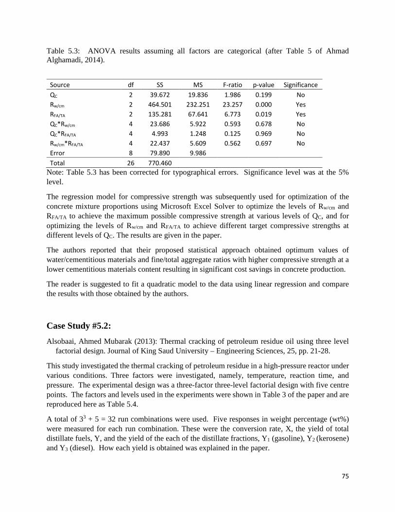
75
Table 5.3: ANOVA results assuming all factors are categorical (after Table 5 of Ahmad Alghamadi, 2014).
Source df SS MS F-ratio p-value Significance QC 2 39.672 19.836 1.986 0.199 No Rw/cm 2 464.501 232.251 23.257 0.000 Yes RFA/TA 2 135.281 67.641 6.773 0.019 Yes QC*Rw/cm 4 23.686 5.922 0.593 0.678 No QC*RFA/TA 4 4.993 1.248 0.125 0.969 No Rw/cm*RFA/TA 4 22.437 5.609 0.562 0.697 No Error 8 79.890 9.986 Total 26 770.460
Note: Table 5.3 has been corrected for typographical errors. Significance level was at the 5% level.
The regression model for compressive strength was subsequently used for optimization of the concrete mixture proportions using Microsoft Excel Solver to optimize the levels of Rw/cm and RFA/TA to achieve the maximum possible compressive strength at various levels of QC, and for optimizing the levels of Rw/cm and RFA/TA to achieve different target compressive strengths at different levels of QC. The results are given in the paper.
The authors reported that their proposed statistical approach obtained optimum values of water/cementitious materials and fine/total aggregate ratios with higher compressive strength at a lower cementitious materials content resulting in significant cost savings in concrete production.
The reader is suggested to fit a quadratic model to the data using linear regression and compare the results with those obtained by the authors.
Case Study #5.2:
Alsobaai, Ahmed Mubarak (2013): Thermal cracking of petroleum residue oil using three level factorial design. Journal of King Saud University – Engineering Sciences, 25, pp. 21-28.
This study investigated the thermal cracking of petroleum residue in a high-pressure reactor under various conditions. Three factors were investigated, namely, temperature, reaction time, and pressure. The experimental design was a three-factor three-level factorial design with five centre points. The factors and levels used in the experiments were shown in Table 3 of the paper and are reproduced here as Table 5.4.
A total of 33 + 5 = 32 run combinations were used. Five responses in weight percentage (wt%) were measured for each run combination. These were the conversion rate, X, the yield of total distillate fuels, Y, and the yield of the each of the distillate fractions, Y1 (gasoline), Y2 (kerosene) and Y3 (diesel). How each yield is obtained was explained in the paper.
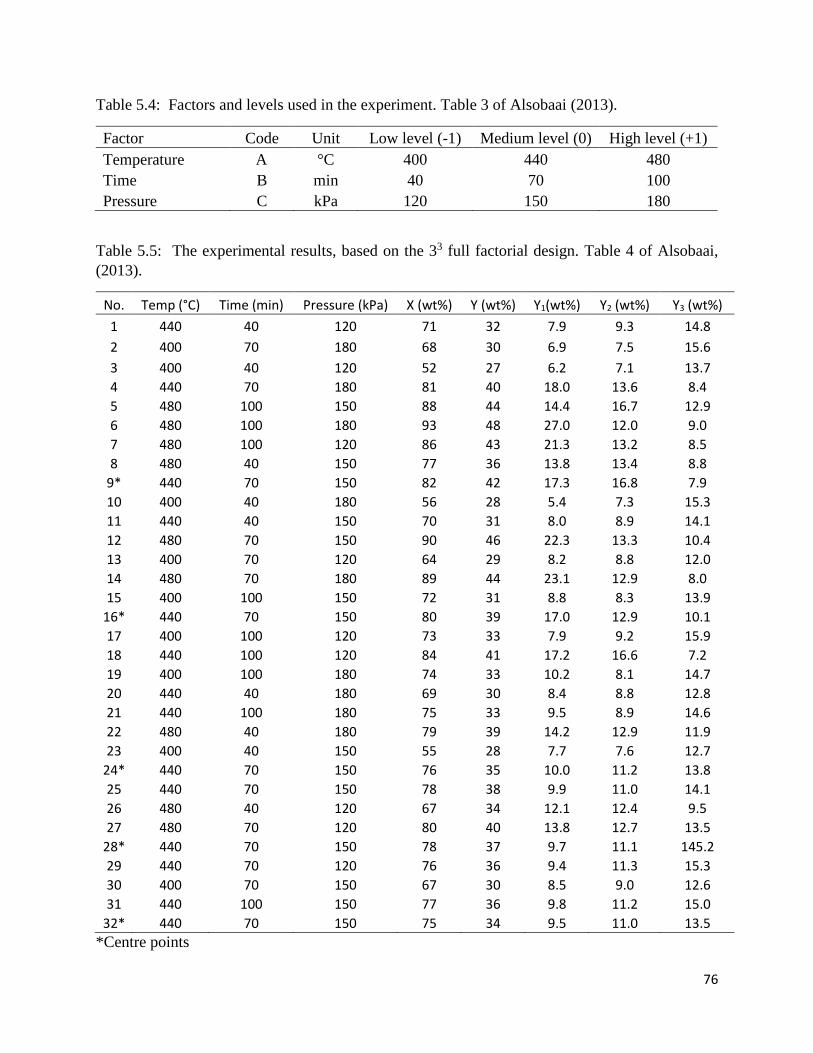
76
Table 5.4: Factors and levels used in the experiment. Table 3 of Alsobaai (2013).
Factor Code Unit Low level (-1) Medium level (0) High level (+1) Temperature A °C 400 440 480 Time B min 40 70 100 Pressure C kPa 120 150 180
Table 5.5: The experimental results, based on the 33 full factorial design. Table 4 of Alsobaai, (2013).
No. Temp (°C) Time (min) Pressure (kPa) X (wt%) Y (wt%) Y1(wt%) Y2 (wt%) Y3 (wt%) 1 440 40 120 71 32 7.9 9.3 14.8 2 400 70 180 68 30 6.9 7.5 15.6 3 400 40 120 52 27 6.2 7.1 13.7 4 440 70 180 81 40 18.0 13.6 8.4 5 480 100 150 88 44 14.4 16.7 12.9 6 480 100 180 93 48 27.0 12.0 9.0 7 480 100 120 86 43 21.3 13.2 8.5 8 480 40 150 77 36 13.8 13.4 8.8
9* 440 70 150 82 42 17.3 16.8 7.9 10 400 40 180 56 28 5.4 7.3 15.3 11 440 40 150 70 31 8.0 8.9 14.1 12 480 70 150 90 46 22.3 13.3 10.4 13 400 70 120 64 29 8.2 8.8 12.0 14 480 70 180 89 44 23.1 12.9 8.0 15 400 100 150 72 31 8.8 8.3 13.9
16* 440 70 150 80 39 17.0 12.9 10.1 17 400 100 120 73 33 7.9 9.2 15.9 18 440 100 120 84 41 17.2 16.6 7.2 19 400 100 180 74 33 10.2 8.1 14.7 20 440 40 180 69 30 8.4 8.8 12.8 21 440 100 180 75 33 9.5 8.9 14.6 22 480 40 180 79 39 14.2 12.9 11.9 23 400 40 150 55 28 7.7 7.6 12.7
24* 440 70 150 76 35 10.0 11.2 13.8 25 440 70 150 78 38 9.9 11.0 14.1 26 480 40 120 67 34 12.1 12.4 9.5 27 480 70 120 80 40 13.8 12.7 13.5
28* 440 70 150 78 37 9.7 11.1 145.2 29 440 70 120 76 36 9.4 11.3 15.3 30 400 70 150 67 30 8.5 9.0 12.6 31 440 100 150 77 36 9.8 11.2 15.0
32* 440 70 150 75 34 9.5 11.0 13.5 *Centre points

77
Statistical analyses were carried out using Design-Expert 6.0.3. A general second-order response surface model was fitted to each of the responses.
The ANOVA results are shown in Tables 5 to 9 of the paper, for X, Y, Y1, Y2, and Y3, respectively. Except for the conversion, X, no goodness-of-fit statistic was given for the other responses in the paper. There is also no mention of whether the assumptions of ANOVA were fulfilled for each of the responses analyzed.
The ANOVA results for the conversion, X, are shown below in Table 5.6 which is adapted from Table 5 of the paper.
Table 5.6: ANOVA results for conversion, X, (wt%).
Source of variation
Sum Squares DF
Mean Square F-value Prob>F Comment
Model 2729.05 9 303.23 27.25 <0.0001 Significant A 1568.00 1 1568.00 140.90 <0.0001 B 882.00 1 882.00 79.26 <0.0001 C 53.39 1 53.39 4.80 0.0394 A2 20.26 1 20.26 1.82 0.1910 B2 97.03 1 97.03 8.72 0.0074 C2 1.91 1 1.91 0.17 0.6830 AB 12.00 1 12.00 1.08 0.3103 AC 30.08 1 30.08 2.70 0.1144 BC 18.75 1 18.75 1.68 0.2077 Residual 244.82 22 11.13 Lack of fit 211.99 17 12.47 1.90 0.2469 Not significant Pure error 32.83 5 6.57 Corr. Total 2973.88 31
The author reported that the full quadratic model has a R2 value of 0.9177, a PRESS of 578.91, and predicted R2 of 0.8053 which is in reasonable agreement with the adjusted R2 of 0.8840. Goodness-of-fit statistics were not given for the reduced model with only statistically significant terms.
The other ANOVA results are given in the paper and will not be reproduced here. The proposed prediction equations in actual factors for X, Y, Y1, Y2, and Y3 are given In Equations (5) – (9) of the paper. They are reproduced here showing the actual factors.
X = Conversion = -238.979 + 0.0193 Temp + 1.3812 Time – 0.2538 Pressure – 0.00409 Time2
Y = Total distilled fuels = -38.4896 + 0.1458 Temp + 0.1056 Time + 0.0185 Pressure
Y1 = Gasoline yield = -54.7414 + 0.1281 Temp + 0.0785 Time + 0.0346 Pressure
Y2 = Kerosene yield = -17.1340 + 0.064722 Temp + 0.0306 Time – 0.0159 Pressure
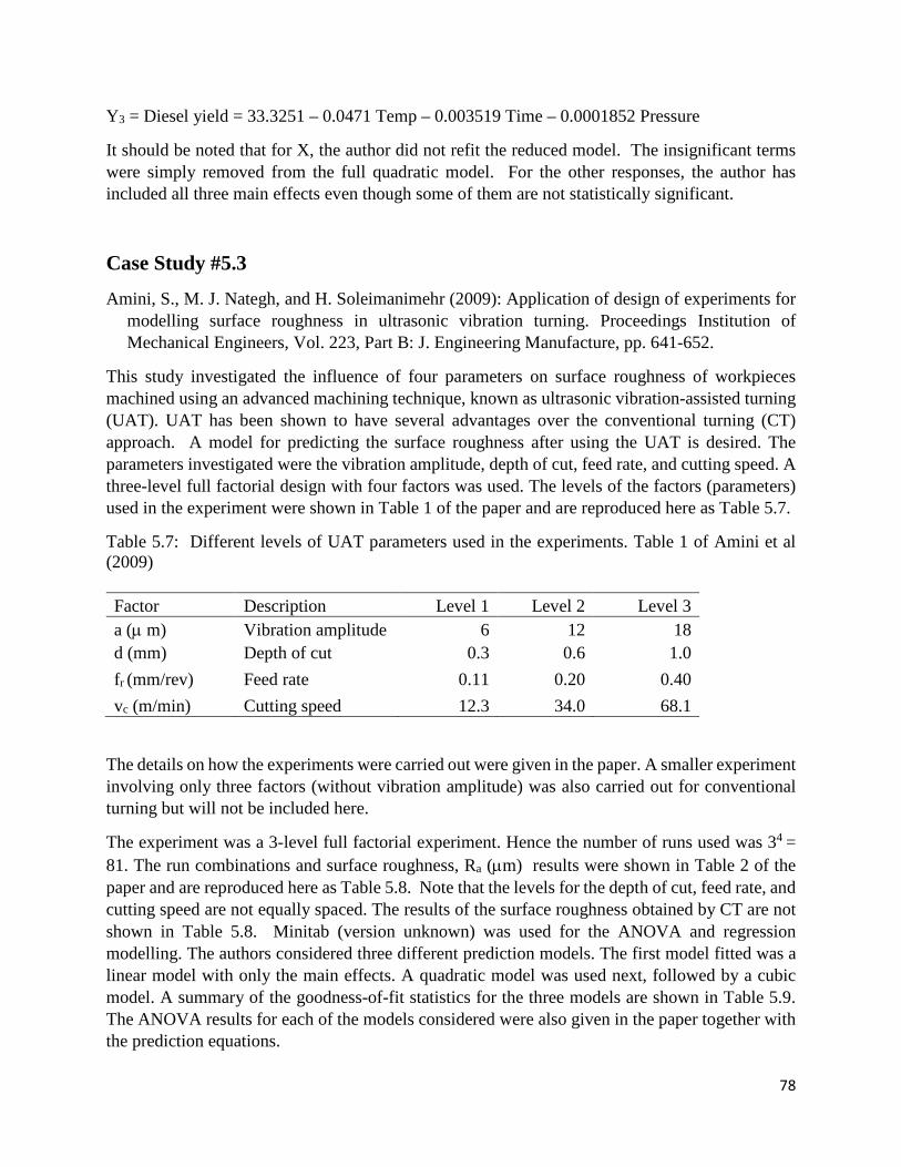
78
Y3 = Diesel yield = 33.3251 – 0.0471 Temp – 0.003519 Time – 0.0001852 Pressure
It should be noted that for X, the author did not refit the reduced model. The insignificant terms were simply removed from the full quadratic model. For the other responses, the author has included all three main effects even though some of them are not statistically significant.
Case Study #5.3
Amini, S., M. J. Nategh, and H. Soleimanimehr (2009): Application of design of experiments for modelling surface roughness in ultrasonic vibration turning. Proceedings Institution of Mechanical Engineers, Vol. 223, Part B: J. Engineering Manufacture, pp. 641-652.
This study investigated the influence of four parameters on surface roughness of workpieces machined using an advanced machining technique, known as ultrasonic vibration-assisted turning (UAT). UAT has been shown to have several advantages over the conventional turning (CT) approach. A model for predicting the surface roughness after using the UAT is desired. The parameters investigated were the vibration amplitude, depth of cut, feed rate, and cutting speed. A three-level full factorial design with four factors was used. The levels of the factors (parameters) used in the experiment were shown in Table 1 of the paper and are reproduced here as Table 5.7.
Table 5.7: Different levels of UAT parameters used in the experiments. Table 1 of Amini et al (2009) Factor Description Level 1 Level 2 Level 3 a (µ m) Vibration amplitude 6 12 18 d (mm) Depth of cut 0.3 0.6 1.0 fr (mm/rev) Feed rate 0.11 0.20 0.40 vc (m/min) Cutting speed 12.3 34.0 68.1
The details on how the experiments were carried out were given in the paper. A smaller experiment involving only three factors (without vibration amplitude) was also carried out for conventional turning but will not be included here.
The experiment was a 3-level full factorial experiment. Hence the number of runs used was 34 = 81. The run combinations and surface roughness, Ra (µm) results were shown in Table 2 of the paper and are reproduced here as Table 5.8. Note that the levels for the depth of cut, feed rate, and cutting speed are not equally spaced. The results of the surface roughness obtained by CT are not shown in Table 5.8. Minitab (version unknown) was used for the ANOVA and regression modelling. The authors considered three different prediction models. The first model fitted was a linear model with only the main effects. A quadratic model was used next, followed by a cubic model. A summary of the goodness-of-fit statistics for the three models are shown in Table 5.9. The ANOVA results for each of the models considered were also given in the paper together with the prediction equations.

79
Table 5.8: Run combinations and UAT surface roughness results. Table 2 of Amini et al (2009).
No. a (µm) d (mm) fr(mm/rev) vc (m/min) Ra (µm) 1 6 0.3 0.11 12.3 0.404 2 6 0.3 0.11 34.0 0.534 3 6 0.3 0.11 68.1 1.546
4 6 0.3 0.20 12.3 1.592
5 6 0.3 0.20 34.0 2.695 6 6 0.3 0.20 68.1 3.090 7 6 0.3 0.40 12.3 6.237 8 6 0.3 0.40 34.0 7.396 9 6 0.3 0.40 68.1 7.401
10 6 0.6 0.11 12.3 2.215 11 6 0.6 0.11 34.0 2.837 12 6 0.6 0.11 68.1 3.142 13 6 0.6 0.20 12.3 2.872 14 6 0.6 0.20 34.0 4.614 15 6 0.6 0.20 68.1 3.047 16 6 0.6 0.40 12.3 6.811 17 6 0.6 0.40 34.0 7.499 18 6 0.6 0.40 68.1 5.700 19 6 1.0 0.11 12.3 2.293 20 6 1.0 0.11 34.0 2.187 21 6 1.0 0.11 68.1 3.292 22 6 1.0 0.20 12.3 2.365 23 6 1.0 0.20 34.0 2.982 24 6 1.0 0.20 68.1 3.543 25 6 1.0 0.40 12.3 5.763 26 6 1.0 0.40 34.0 5.631 27 6 1.0 0.40 68.1 6.479 28 12 0.3 0.11 12.3 0.683 29 12 0.3 0.11 34.0 0.868 30 12 0.3 0.11 68.1 0.971 31 12 0.3 0.20 12.3 1.914 32 12 0.3 0.20 34.0 1.713 33 12 0.3 0.20 68.1 1.715 34 12 0.3 0.40 12.3 6.429 35 12 0.3 0.40 34.0 5.927 36 12 0.3 0.40 68.1 6.057 37 12 0.6 0.11 12.3 0.596 38 12 0.6 0.11 34.0 0.752 39 12 0.6 0.11 68.1 0.790

80
No. a (µm) d (mm) fr(mm/rev) vc (m/min) Ra (µm) 40 12 0.6 0.20 12.3 1.595 41 12 0.6 0.20 34.0 1.644 42 12 0.6 0.20 68.1 1.889 43 12 0.6 0.40 12.3 6.808 44 12 0.6 0.40 34.0 5.636 45 12 0.6 0.40 68.1 5.980 46 12 1.0 0.11 12.3 0.788 47 12 1.0 0.11 34.0 0.763 48 12 1.0 0.11 68.1 0.840 49 12 1.0 0.20 12.3 1.750 50 12 1.0 0.20 34.0 1.906 51 12 1.0 0.20 68.1 1.757 52 12 1.0 0.40 12.3 6.700 53 12 1.0 0.40 34.0 6.955 54 12 1.0 0.40 68.1 6.616 55 18 0.3 0.11 12.3 1.330 56 18 0.3 0.11 34.0 1.855 57 18 0.3 0.11 68.1 0.729 58 18 0.3 0.20 12.3 1.645 59 18 0.3 0.20 34.0 2.948 60 18 0.3 0.20 68.1 2.180 61 18 0.3 0.40 12.3 4.910 62 18 0.3 0.40 34.0 6.404 63 18 0.3 0.40 68.1 7.155 64 18 0.6 0.11 12.3 2.885 65 18 0.6 0.11 34.0 0.743 66 18 0.6 0.11 68.1 0.774 67 18 0.6 0.20 12.3 2.812 68 18 0.6 0.20 34.0 2.295 69 18 0.6 0.20 68.1 1.682 70 18 0.6 0.40 12.3 6.311 71 18 0.6 0.40 34.0 6.664 72 18 0.6 0.40 68.1 6.148 73 18 1.0 0.11 12.3 1.530 74 18 1.0 0.11 34.0 1.501 75 18 1.0 0.11 68.1 1.371 76 18 1.0 0.20 12.3 2.580 77 18 1.0 0.20 34.0 2.134 78 18 1.0 0.20 68.1 2.252 79 18 1.0 0.40 12.3 7.595 80 18 1.0 0.40 34.0 7.615 81 18 1.0 0.40 68.1 8.019
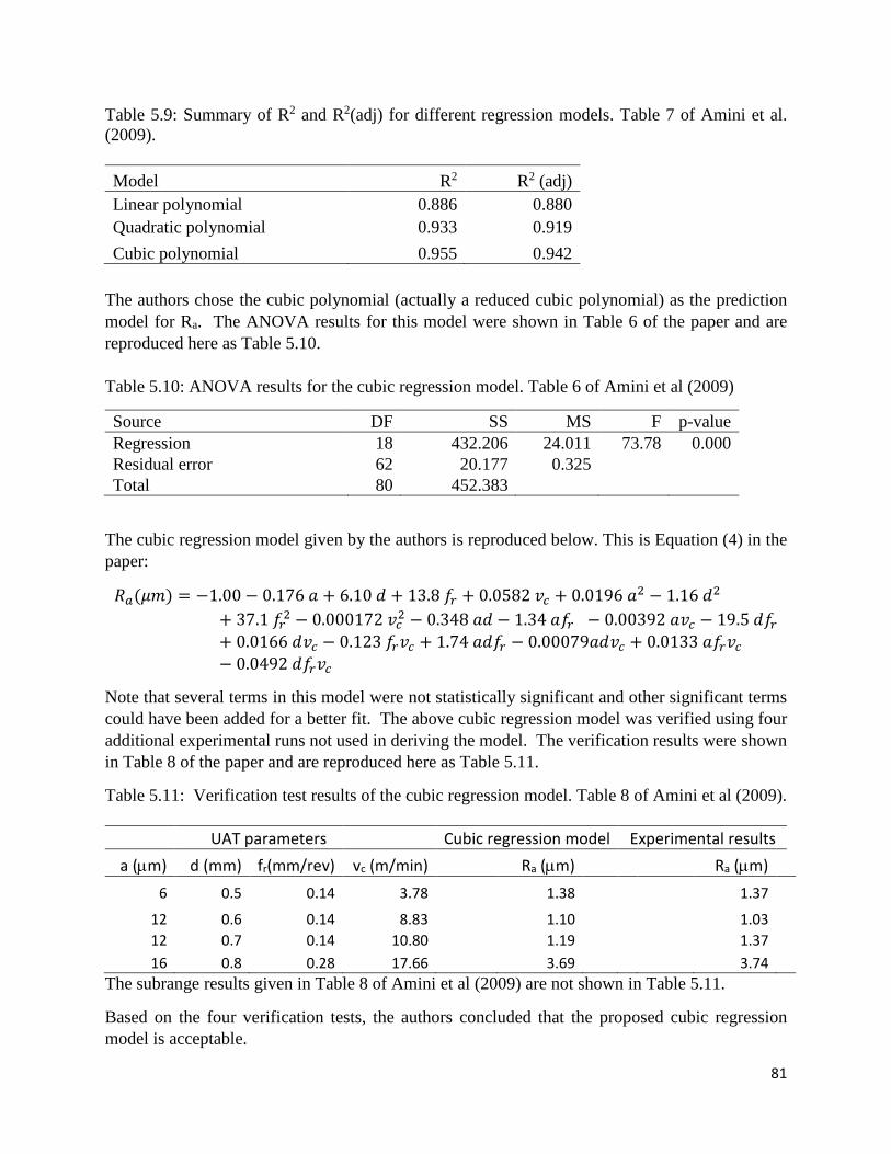
81
Table 5.9: Summary of R2 and R2(adj) for different regression models. Table 7 of Amini et al. (2009). Model R2 R2 (adj) Linear polynomial 0.886 0.880 Quadratic polynomial 0.933 0.919 Cubic polynomial 0.955 0.942
The authors chose the cubic polynomial (actually a reduced cubic polynomial) as the prediction model for Ra. The ANOVA results for this model were shown in Table 6 of the paper and are reproduced here as Table 5.10. Table 5.10: ANOVA results for the cubic regression model. Table 6 of Amini et al (2009)
Source DF SS MS F p-value Regression 18 432.206 24.011 73.78 0.000 Residual error 62 20.177 0.325 Total 80 452.383
The cubic regression model given by the authors is reproduced below. This is Equation (4) in the paper:
𝑅𝑅𝑎𝑎(𝜇𝜇𝜇𝜇) = −1.00 − 0.176 𝑎𝑎 + 6.10 𝑑𝑑 + 13.8 𝑓𝑓𝑟𝑟 + 0.0582 𝑣𝑣𝑐𝑐 + 0.0196 𝑎𝑎2 − 1.16 𝑑𝑑2
+ 37.1 𝑓𝑓𝑟𝑟2 − 0.000172 𝑣𝑣𝑐𝑐2 − 0.348 𝑎𝑎𝑑𝑑 − 1.34 𝑎𝑎𝑓𝑓𝑟𝑟 − 0.00392 𝑎𝑎𝑣𝑣𝑐𝑐 − 19.5 𝑑𝑑𝑓𝑓𝑟𝑟+ 0.0166 𝑑𝑑𝑣𝑣𝑐𝑐 − 0.123 𝑓𝑓𝑟𝑟𝑣𝑣𝑐𝑐 + 1.74 𝑎𝑎𝑑𝑑𝑓𝑓𝑟𝑟 − 0.00079𝑎𝑎𝑑𝑑𝑣𝑣𝑐𝑐 + 0.0133 𝑎𝑎𝑓𝑓𝑟𝑟𝑣𝑣𝑐𝑐− 0.0492 𝑑𝑑𝑓𝑓𝑟𝑟𝑣𝑣𝑐𝑐
Note that several terms in this model were not statistically significant and other significant terms could have been added for a better fit. The above cubic regression model was verified using four additional experimental runs not used in deriving the model. The verification results were shown in Table 8 of the paper and are reproduced here as Table 5.11.
Table 5.11: Verification test results of the cubic regression model. Table 8 of Amini et al (2009).
UAT parameters Cubic regression model Experimental results a (µm) d (mm) fr(mm/rev) vc (m/min) Ra (µm) Ra (µm)
6 0.5 0.14 3.78 1.38 1.37 12 0.6 0.14 8.83 1.10 1.03 12 0.7 0.14 10.80 1.19 1.37 16 0.8 0.28 17.66 3.69 3.74
The subrange results given in Table 8 of Amini et al (2009) are not shown in Table 5.11.
Based on the four verification tests, the authors concluded that the proposed cubic regression model is acceptable.
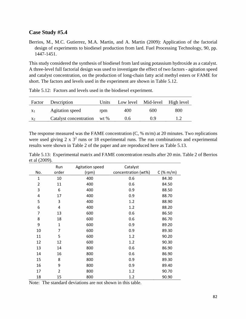
82
Case Study #5.4
Berrios, M., M.C. Gutierrez, M.A. Martin, and A. Martin (2009): Application of the factorial design of experiments to biodiesel production from lard. Fuel Processing Technology, 90, pp. 1447-1451.
This study considered the synthesis of biodiesel from lard using potassium hydroxide as a catalyst. A three-level full factorial design was used to investigate the effect of two factors - agitation speed and catalyst concentration, on the production of long-chain fatty acid methyl esters or FAME for short. The factors and levels used in the experiment are shown in Table 5.12.
Table 5.12: Factors and levels used in the biodiesel experiment.
Factor Description Units Low level Mid-level High level
x1 Agitation speed rpm 400 600 800 x2 Catalyst concentration wt % 0.6 0.9 1.2
The response measured was the FAME concentration (C, % m/m) at 20 minutes. Two replications were used giving 2 x 32 runs or 18 experimental runs. The run combinations and experimental results were shown in Table 2 of the paper and are reproduced here as Table 5.13.
Table 5.13: Experimental matrix and FAME concentration results after 20 min. Table 2 of Berrios et al (2009).
No. Run
order Agitation speed
(rpm) Catalyst
concentration (wt%) C (% m/m) 1 10 400 0.6 84.30 2 11 400 0.6 84.50 3 6 400 0.9 88.50 4 17 400 0.9 88.70 5 3 400 1.2 88.90 6 4 400 1.2 88.20 7 13 600 0.6 86.50 8 18 600 0.6 86.70 9 1 600 0.9 89.20
10 7 600 0.9 89.30 11 5 600 1.2 90.20 12 12 600 1.2 90.30 13 14 800 0.6 86.90 14 16 800 0.6 86.90 15 8 800 0.9 89.30 16 9 800 0.9 89.40 17 2 800 1.2 90.70 18 15 800 1.2 90.90
Note: The standard deviations are not shown in this table.
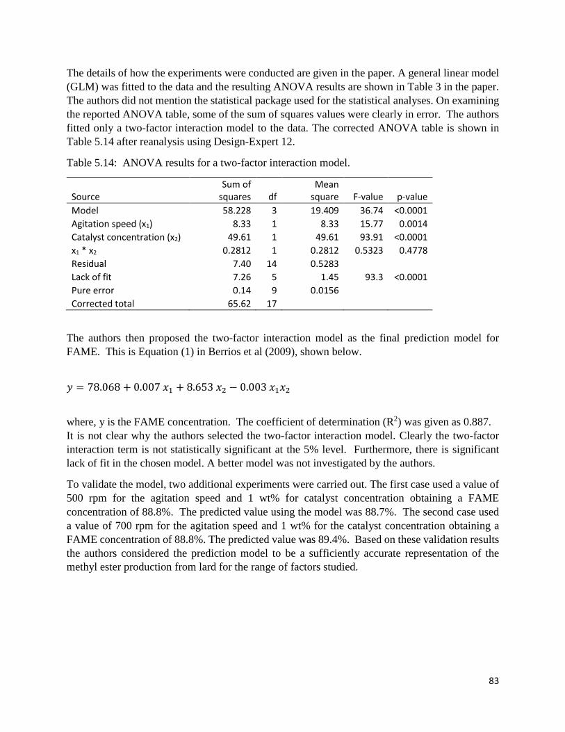
83
The details of how the experiments were conducted are given in the paper. A general linear model (GLM) was fitted to the data and the resulting ANOVA results are shown in Table 3 in the paper. The authors did not mention the statistical package used for the statistical analyses. On examining the reported ANOVA table, some of the sum of squares values were clearly in error. The authors fitted only a two-factor interaction model to the data. The corrected ANOVA table is shown in Table 5.14 after reanalysis using Design-Expert 12.
Table 5.14: ANOVA results for a two-factor interaction model.
Source Sum of
squares df Mean
square F-value p-value Model 58.228 3 19.409 36.74 <0.0001 Agitation speed (x1) 8.33 1 8.33 15.77 0.0014 Catalyst concentration (x2) 49.61 1 49.61 93.91 <0.0001 x1 * x2 0.2812 1 0.2812 0.5323 0.4778 Residual 7.40 14 0.5283 Lack of fit 7.26 5 1.45 93.3 <0.0001 Pure error 0.14 9 0.0156 Corrected total 65.62 17
The authors then proposed the two-factor interaction model as the final prediction model for FAME. This is Equation (1) in Berrios et al (2009), shown below.
𝑦𝑦 = 78.068 + 0.007 𝐸𝐸1 + 8.653 𝐸𝐸2 − 0.003 𝐸𝐸1𝐸𝐸2
where, y is the FAME concentration. The coefficient of determination (R2) was given as 0.887. It is not clear why the authors selected the two-factor interaction model. Clearly the two-factor interaction term is not statistically significant at the 5% level. Furthermore, there is significant lack of fit in the chosen model. A better model was not investigated by the authors.
To validate the model, two additional experiments were carried out. The first case used a value of 500 rpm for the agitation speed and 1 wt% for catalyst concentration obtaining a FAME concentration of 88.8%. The predicted value using the model was 88.7%. The second case used a value of 700 rpm for the agitation speed and 1 wt% for the catalyst concentration obtaining a FAME concentration of 88.8%. The predicted value was 89.4%. Based on these validation results the authors considered the prediction model to be a sufficiently accurate representation of the methyl ester production from lard for the range of factors studied.

84
Case Study #5.5
Comoglu, B. A., Cansun Filik Iscen, and Semra IIhan (2015): The anaerobic treatment of pharmaceutical industry wastewater in an anaerobic batch and upflow packed-bed reactor. Desalination and Water Treatment, 2015, pp 1-12.
This study concerned the treatment of pharmaceutical industry wastewater before discharge into receiving water bodies. Pharmaceutical industry wastewater is known to contain various complex organic chemicals that are toxic to the environment. One of the experiments investigated the effect of three factors, namely, basal medium, wastewater concentration, and various types of co-substrate, on COD removal. A three-level full factorial design with three factors was used. The factors and levels used in the experiment were shown in Table 1 of the paper and are reproduced here as Table 5.15.
Table 5.15: Variables and levels used in the experimental design. Table 1 of Comoglu et al ( 2015) Levels Variables -1 0 1 X1 - Basal medium (%) 5 10 15 X2 - Wastewater (%) 25 50 75 X3 - Cosubstrate type Propionic acid Glucose Acid mix
Since this was a 33 full factorial experiment, 27 runs were required. The basal medium and wastewater concentrations are numeric factors while the co-substrate type is a categorical factor. The co-substrate is one of three types. The first type is a mixture of acetic-propionic-butyric acids or (ABP), each at various concentrations. The second type is glucose, and the third type is propionic acid. The other details of the experiment were given in the paper.
The response variable was the percentage of COD removed from the wastewater stream. The experiments were carried out in a batch reactor. The 27 run combinations of the experiment together with the COD removal percentage is shown in Table 2.16 which is Table 2 in the paper. All experiments were performed in duplicate but only 27 responses were given in the paper.
Statistical analyses were carried out using the SPSS statistical package. The ANOVA results and multiple comparison tests results were given in Tables 3 and 4 of the paper and are reproduced here as Table 5.17.
From the ANOVA results, the authors have treated all factors as categorical and the corrected sum of squares degrees of freedom is shown as 53, indicating that there were 54 data points used in the ANOVA. Hence the results given in Table 5.17 (Table 2 in the paper) were incomplete.
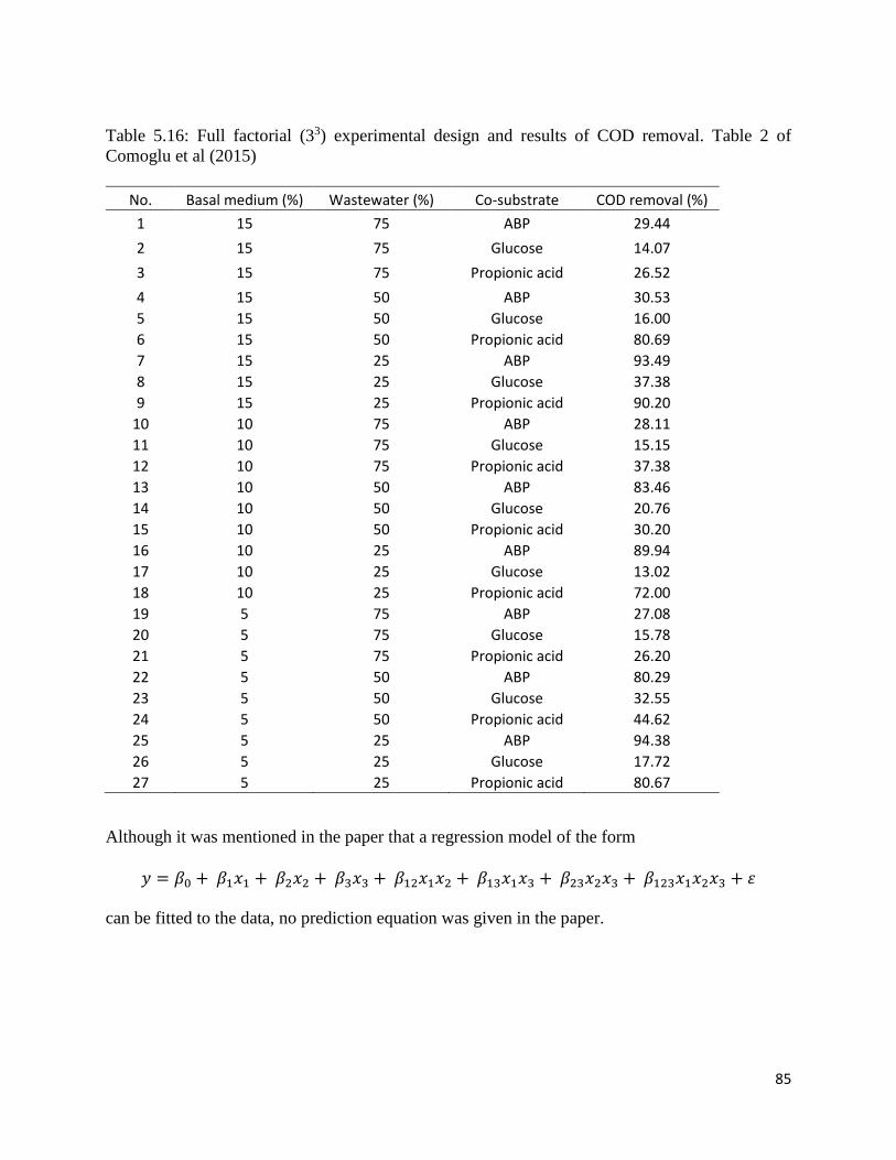
85
Table 5.16: Full factorial (33) experimental design and results of COD removal. Table 2 of Comoglu et al (2015)
No. Basal medium (%) Wastewater (%) Co-substrate COD removal (%) 1 15 75 ABP 29.44 2 15 75 Glucose 14.07 3 15 75 Propionic acid 26.52 4 15 50 ABP 30.53 5 15 50 Glucose 16.00 6 15 50 Propionic acid 80.69 7 15 25 ABP 93.49 8 15 25 Glucose 37.38 9 15 25 Propionic acid 90.20
10 10 75 ABP 28.11 11 10 75 Glucose 15.15 12 10 75 Propionic acid 37.38 13 10 50 ABP 83.46 14 10 50 Glucose 20.76 15 10 50 Propionic acid 30.20 16 10 25 ABP 89.94 17 10 25 Glucose 13.02 18 10 25 Propionic acid 72.00 19 5 75 ABP 27.08 20 5 75 Glucose 15.78 21 5 75 Propionic acid 26.20 22 5 50 ABP 80.29 23 5 50 Glucose 32.55 24 5 50 Propionic acid 44.62 25 5 25 ABP 94.38 26 5 25 Glucose 17.72 27 5 25 Propionic acid 80.67
Although it was mentioned in the paper that a regression model of the form
𝑦𝑦 = 𝛽𝛽0 + 𝛽𝛽1𝐸𝐸1 + 𝛽𝛽2𝐸𝐸2 + 𝛽𝛽3𝐸𝐸3 + 𝛽𝛽12𝐸𝐸1𝐸𝐸2 + 𝛽𝛽13𝐸𝐸1𝐸𝐸3 + 𝛽𝛽23𝐸𝐸2𝐸𝐸3 + 𝛽𝛽123𝐸𝐸1𝐸𝐸2𝐸𝐸3 + 𝜀𝜀 can be fitted to the data, no prediction equation was given in the paper.

86
Table 5.17: Variance analysis for COD removal. Table 3 of Comoglu et al (2015) Source Type III SS df MS F p-value Corrected model 45969.788 26 1768.069 13.629 0.000* Intercept 111623.395 1 111623.395 860.416 0.000* Basal 122.962 2 61.481 0.474 0.628 Wastewater 15165.682 2 7582.841 58.450 0.000* Co-substrate 17659.762 2 8829.881 68.063 0.000* Basal-wastewater 985.515 4 246.379 1.899 0.140 Basal-cosubstrate 2293.123 4 573.281 4.419 0.007* Wastewater-cosubstrate 5432.023 4 1358.006 10.468 0.000* Basal-wastewater-cosubstrate 4310.76 8 538.845 4.154 0.002* Error 3502.76 27 129.732 Total 161095.943 54 Corrected total 49472.548 53
Based on the ANOVA results, with the exception of the basal medium, the authors reported that the other factors and two-way interactions between basal and co-substrate, wastewater and co-substrate, and the three-way interaction among the three factors were statistically significant at the 5% level.
In view of the missing duplicate data, it is not possible to replicate the authors’ results. There was also no mention of whether the assumptions of ANOVA were fulfilled.
Case Study #5.6
Martin-Lara, M. A., I. L. Rodriguez, G. Blazquez, and M. Calero (2011): Factorial experimental design for optimizing the removal conditions of lead ions from aqueous solutions by three wastes of olive-oil production. Desalination, 278, pp. 132-140.
Three wastes, namely olive stone (OS), two-phase olive solid (OMS), and olive tree pruning waste (OTP), from olive-oil production were considered as low-cost adsorbents for lead removal from aqueous solutions. Two sets of three-level factorial design each with two factors were used for each biosorbent. The factors studied were biosorbent dosage and pH for the first set of experiments, and initial lead concentration and temperature for the second of experiments. The factors and levels used were shown in Table 1 of the paper and reproduced here as Table 5.18.
The responses measured were lead removal percentage and biosorption capacity after 120 minutes of contact time for each of OS, OMS, and OTP. The experimental details were given in the paper and statistical analyses were carried out using Statgraphics Plus 5.1 software.
The run combinations and the results for lead uptake by OS, OMS, and OTP using the factors biosorbent dosage (g/L) and pH in the first set of experiments were shown in Table 2 of the paper

87
and reproduced here as Table 5.19. For the second set of experiments, the run combinations and results were shown in Table 4 of the paper and are reproduced here as Table 5.20. The same responses were used but with the initial lead concentration and temperature as factors. The experiments were run in random order and in duplicate. Hence there were 2 x 32 = 18 runs per response.
Table 5.18: Factors and levels used in the experimental design. Table 1 of Martin-Lara et al (2011) Factor Symbol Low level Center level High level (-1) (0) (+1) Biosorbent dosage, g/L X1 2 10 22 pH X2 4 5 6 [Pb]initial, mg/L X3 10 40 70 Temperature, C X4 25 40 60
Note: only X1 and X2 were used in the first set of experiments, and only X3 and X4 were used in the second set of experiments. Some of the factor levels are not equally spaced.
Table 5.19: First experimental factorial design for lead uptake by OS, OMS, and OTP. Table 2 of Martin-Lara et al (2011).
Note: The factors in Table 5.19 and 5.20 are listed here as actual factors instead of coded factors in Tables 2 and 3 of the paper.
RunTwo-phase olive mill solid (OMS)
Biosorbent pH Removal (%) Biosorption Removal (%) Biosorption Removal (%) Biosorption
dosage capacity (mg/g) capacity (mg/g) capacity (mg/g)1 2 4 29.00 1.450 57.30 2.865 90.00 4.5002 10 4 69.42 0.694 88.90 0.889 97.00 0.9703 22 4 73.30 0.333 87.00 0.395 93.50 0.4254 2 5 49.80 2.490 52.50 2.625 92.00 4.6005 10 5 77.30 0.773 83.40 0.834 98.00 0.9806 22 5 76.00 0.345 88.40 0.402 94.60 0.4307 2 6 69.90 3.495 61.90 3.095 89.80 4.4908 10 6 79.80 0.798 88.04 0.880 96.60 0.9669 22 6 79.10 0.360 85.10 0.387 95.00 0.432
10 2 4 28.35 1.418 56.70 2.835 89.60 4.48011 10 4 68.20 0.682 88.10 0.881 96.40 0.96412 22 4 72.90 0.331 86.60 0.394 92.10 0.41913 2 5 48.90 2.445 51.50 2.575 91.40 4.57014 10 5 77.10 0.771 82.60 0.826 97.80 0.97815 22 5 75.00 0.341 88.00 0.400 94.00 0.42716 2 6 69.10 3.455 62.10 3.105 89.40 4.47017 10 6 79.40 0.794 87.20 0.872 96.40 0.96418 22 6 79.20 0.360 84.90 0.386 94.40 0.430
Olive Stone (OS)Factors Biosorbent
Olive tree pruning (OTP)

88
Table 5.20: Second experimental factorial design for lead uptake by OS, OMS, and OTP. Table 4 of Martin-Lara et al (2011).
Second-order response surface models with two independent variables (Xi and Xj) were fitted to each of the responses. The model is of the form:
𝑌𝑌 = 𝑏𝑏0 + 𝑏𝑏𝑖𝑖𝑋𝑋𝑖𝑖 + 𝑏𝑏𝑗𝑗𝑋𝑋𝑗𝑗 + 𝑏𝑏𝑖𝑖𝑖𝑖𝑋𝑋𝑖𝑖2 + 𝑏𝑏𝑗𝑗𝑗𝑗𝑋𝑋𝑗𝑗2 + 𝑏𝑏𝑖𝑖𝑗𝑗𝑋𝑋𝑖𝑖𝑋𝑋𝑗𝑗
where, i and j are 1 and 2, respectively for the first set of experiments, and 3 and 4, respectively, for the second set of experiments. Note that in the paper, the models for the second set of experiments were erroneously stated in terms of 1 and 2 instead of 3 and 4.
The models’ coefficients for each response were tabulated by the authors in Tables 3 and 5 for the first and second set of experiments, respectively. These are reproduced here with corrections as Tables 5.21 and 5.22. There was no indication if there was lack of fit or if the assumptions of regression were checked. The R2 values reported were for the full models only. Some of the responses should have been log-transformed.
The authors concluded that the developed regression models for predicting lead removal and lead biosorption capacity fitted the experimental data very well.
RunTwo-phase olive mill solid (OMS)
[Pb]initial Temp Removal (%) Biosorption Removal (%) Biosorption Removal (%) Biosorptioncapacity (mg/g) capacity (mg/g) capacity (mg/g)
1 10 25 77.30 0.773 83.40 0.834 98.00 0.9802 40 25 74.50 2.980 59.02 2.362 90.90 3.6363 70 25 49.07 3.435 44.00 3.080 86.30 6.0414 10 40 73.00 0.730 60.00 0.600 80.60 0.8065 40 40 70.53 2.821 55.25 2.210 88.48 3.5396 70 40 35.17 2.462 38.00 2.660 75.83 5.3087 10 60 76.50 0.765 52.50 0.525 77.00 0.7708 40 60 63.20 2.528 49.48 1.979 87.50 3.5009 70 60 44.46 3.112 37.14 2.600 78.64 5.500
10 10 25 77.10 0.771 82.60 0.826 97.80 0.97811 40 25 74.10 2.964 58.80 2.351 90.88 3.63512 70 25 48.61 3.403 43.89 3.072 86.14 6.03013 10 40 72.20 0.722 58.60 0.586 80.90 0.80914 40 40 70.25 2.810 54.95 2.198 88.20 3.52815 70 40 34.21 2.395 37.87 2.651 75.70 5.29916 10 60 76.10 0.761 51.40 0.514 75.60 0.75617 40 60 63.00 2.520 49.08 1.963 85.90 3.43618 70 60 44.09 3.086 36.91 2.584 78.41 5.489
Olive Stone (OS) Olive tree pruning (OTP)Factors Biosorbent

89
Table 5.21: First experimental design: Response function coefficients for lead removal efficiency and lead biosorption capacity. X1 = biosorbent dosage, and X2 = pH. Table 3 of Martin-Lara et al (2011).
OSCoefficient value Std. Deviation Coefficient value Std. Deviation
b0 -76.1917 8.5174 -1.7152 0.2877X1 b1 9.2517 0.8584 -0.0879 0.0582X2 b2 27.6376 9.6156 1.0245 0.3292X1X2 b12 -0.8163 0.1371 -0.0466 0.0093X2
1 b11 -0.1597 0.0205 0.0090 0.0014X2
2 b22 -0.8775 0.1952 -0.0133 0.0023R2 0.961 0.957Standard error of est. 3.904 0.276Mean absolute error 2.676 0.169
OMSCoefficient value Std. Deviation Coefficient value Std. Deviation
b0 118.2520 31.6512 6.3912 1.3049X1 b1 6.6580 0.5599 -0.3441 0.0231X2 b2 -32.0045 9.7966 -1.2772 0.5276X1X2 b12 -0.1596 0.0894 -0.0059 0.0036X2
1 b11 -0.1824 0.0133 0.0105 0.0006X2
2 b22 3.4200 1.2735 0.1383 0.0525
R2 0.979 0.994Standard error of est. 2.547 0.109Mean absolute error 1.804 0.075
OTPCoefficient value Std. Deviation Coefficient value Std. Deviation
b0 58.7363 7.0036 4.9001 0.3323X1 b1 1.1972 0.1239 -0.6848 0.0058X2 b2 12.2772 2.8315 0.3775 0.1343X1X2 b12 0.0579 0.0197 0.0005 0.0001X2
1 b11 -0.0544 0.0029 0.0199 0.0001X2
2 b22 -1.2667 0.2817 -0.0383 0.0133
R2 0.974 0.999Standard error of est. 0.564 0.027Mean absolute error 0.377 0.018
Removal (%) Biosorption capacity (mg/g)
Removal (%) Biosorption capacity (mg/g)
Removal (%) Biosorption capacity (mg/g)

90
Table 5.22: Second experimental design: Response function coefficients for lead removal efficiency and lead biosorption capacity. X3 = Initial Pb concentration, and X4 = Temperature. Table 5 of Martin-Lara et al (2011).
OSCoefficient value Std. Deviation Coefficient value Std. Deviation
b0 104.7230 11.8844 1.3789 0.6524
X3 b3 0.4254 0.2037 0.1353 0.0111
X4 b4 -1.5689 0.5606 -0.0980 0.0308
X3X4 b34 -0.0014 0.0025 -0.0001 0.00001
X23 b33 -0.0114 0.0021 -0.0012 0.00001
X24 b44 0.0172 0.0063 0.0012 0.00004
R2 0.957 0.974Standard error of est. 3.975 0.210Mean absolute error 2.582 0.147
OMSCoefficient value Std. Deviation Coefficient value Std. Deviation
b0 128.008 10.3377 0.8101 0.1668
X3 b3 -0.6847 0.1772 0.0801 0.0028
X4 b4 -2.1388 0.4877 -0.0369 0.0078
X3X4 b34 0.0112 0.0022 -0.0001 0.00004
X23 b33 -0.0025 0.0018 -0.0005 0.00003
X24 b44 0.0146 0.0063 0.0003 0.00009
R2 0.958 0.998Standard error of est. 3.451 0.055Mean absolute error 2.294 0.034
OTPCoefficient value Std. Deviation Coefficient value Std. Deviation
b0 133.432 9.33940 1.0380 0.4051
X3 b3 0.1845 0.16010 0.1130 0.0069
X4 b4 -2.0751 0.44060 -0.0610 0.0191
X3X4 b34 0.0066 0.00200 -0.0001 0.00009
X23 b33 -0.0067 0.00160 -0.0003 0.00007
X24 b44 0.0176 0.00500 -0.0007 0.0002
R2 0.877 0.997Standard error of est. 3.121 0.136Mean absolute error 2.144 0.091
Removal (%) Biosorption capacity (mg/g)
Removal (%) Biosorption capacity (mg/g)
Removal (%) Biosorption capacity (mg/g)

91
______________________________________________ 6. RSM: BOX BEHNKEN DESIGNS
Eight case studies are presented in this Chapter. The case studies in this Chapter use RSM based on Box-Behnken designs (BBD). The number of factors ranges from three to six. The Box-Behnken design is a well-known classical response surface design with three levels (-1, 0, +1) and there are no extreme combinations of the factors. These designs are rotatable or near rotatable. The main drawback of BBD is that it is not amendable to sequential experimentation unlike central composite designs. These designs require more runs than central composite designs except when the number of factors are three or four.
Case Study #6.1
Aslan, N. and Y. Cebeci (2007): Application of Box-Behnken design and response surface methodology for modeling of Turkish coals. Fuel, 86, pp. 90-97.
This study applied response surface methodology to model the grinding process of some Turkish coals. Steel ball diameter, grinding time, and the Bond work index were three independent factors studied. The Box-Behnken response surface design with three factors was used to obtain the experimental data for statistical analysis and modelling. The importance of studying the grinding process and the materials and methods used were described in the paper.
The factors and levels used for the grinding experiment were shown in Table 4 of the paper and are reproduced here as Table 6.1. Note that in the original table, the levels of the ball diameter were listed as 2.5, 4.0 and 5.5, however, the text and later tables showed that the levels should be 25, 40 and 55, respectively.
Table 6.1: The levels of variables chosen for the Box-Behnken design. Corrected Table 4 of Aslan et al (2007).
The response measured from the experiment was the 80% passing size (d80) in three size fractions (coarse, middle, and fine) of the coal. They were: y1 = -3350 + 1700 (µm), y2 = -1700 + 710 (µm), and y3 = -710 (µm).
Variable SymbolLow (-1) Center (0) High (+1)
Ball diameter d, (mm) x1 25 40 55Grinding time t, (min) x2 2 6 10Bond work index Wi, (kWh/t) x3 12 17 22
Coded variable level
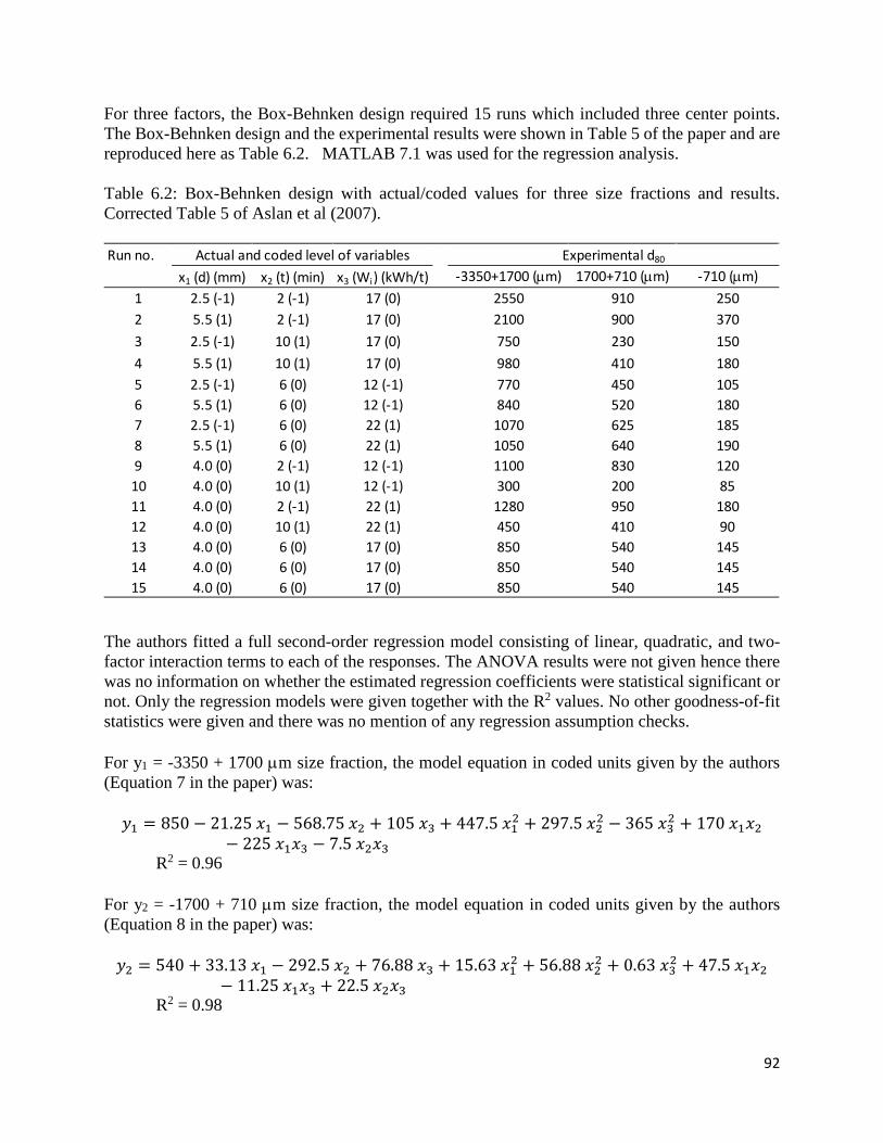
92
For three factors, the Box-Behnken design required 15 runs which included three center points. The Box-Behnken design and the experimental results were shown in Table 5 of the paper and are reproduced here as Table 6.2. MATLAB 7.1 was used for the regression analysis. Table 6.2: Box-Behnken design with actual/coded values for three size fractions and results. Corrected Table 5 of Aslan et al (2007).
The authors fitted a full second-order regression model consisting of linear, quadratic, and two-factor interaction terms to each of the responses. The ANOVA results were not given hence there was no information on whether the estimated regression coefficients were statistical significant or not. Only the regression models were given together with the R2 values. No other goodness-of-fit statistics were given and there was no mention of any regression assumption checks. For y1 = -3350 + 1700 µm size fraction, the model equation in coded units given by the authors (Equation 7 in the paper) was: 𝑦𝑦1 = 850 − 21.25 𝑥𝑥1 − 568.75 𝑥𝑥2 + 105 𝑥𝑥3 + 447.5 𝑥𝑥12 + 297.5 𝑥𝑥22 − 365 𝑥𝑥32 + 170 𝑥𝑥1𝑥𝑥2
− 225 𝑥𝑥1𝑥𝑥3 − 7.5 𝑥𝑥2𝑥𝑥3 R2 = 0.96 For y2 = -1700 + 710 µm size fraction, the model equation in coded units given by the authors (Equation 8 in the paper) was: 𝑦𝑦2 = 540 + 33.13 𝑥𝑥1 − 292.5 𝑥𝑥2 + 76.88 𝑥𝑥3 + 15.63 𝑥𝑥12 + 56.88 𝑥𝑥22 + 0.63 𝑥𝑥32 + 47.5 𝑥𝑥1𝑥𝑥2
− 11.25 𝑥𝑥1𝑥𝑥3 + 22.5 𝑥𝑥2𝑥𝑥3 R2 = 0.98
Run no.x1 (d) (mm) x2 (t) (min) x3 (Wi) (kWh/t) -3350+1700 (µm) 1700+710 (µm) -710 (µm)
1 2.5 (-1) 2 (-1) 17 (0) 2550 910 2502 5.5 (1) 2 (-1) 17 (0) 2100 900 3703 2.5 (-1) 10 (1) 17 (0) 750 230 1504 5.5 (1) 10 (1) 17 (0) 980 410 1805 2.5 (-1) 6 (0) 12 (-1) 770 450 1056 5.5 (1) 6 (0) 12 (-1) 840 520 1807 2.5 (-1) 6 (0) 22 (1) 1070 625 1858 5.5 (1) 6 (0) 22 (1) 1050 640 1909 4.0 (0) 2 (-1) 12 (-1) 1100 830 12010 4.0 (0) 10 (1) 12 (-1) 300 200 8511 4.0 (0) 2 (-1) 22 (1) 1280 950 18012 4.0 (0) 10 (1) 22 (1) 450 410 9013 4.0 (0) 6 (0) 17 (0) 850 540 14514 4.0 (0) 6 (0) 17 (0) 850 540 14515 4.0 (0) 6 (0) 17 (0) 850 540 145
Experimental d80Actual and coded level of variables
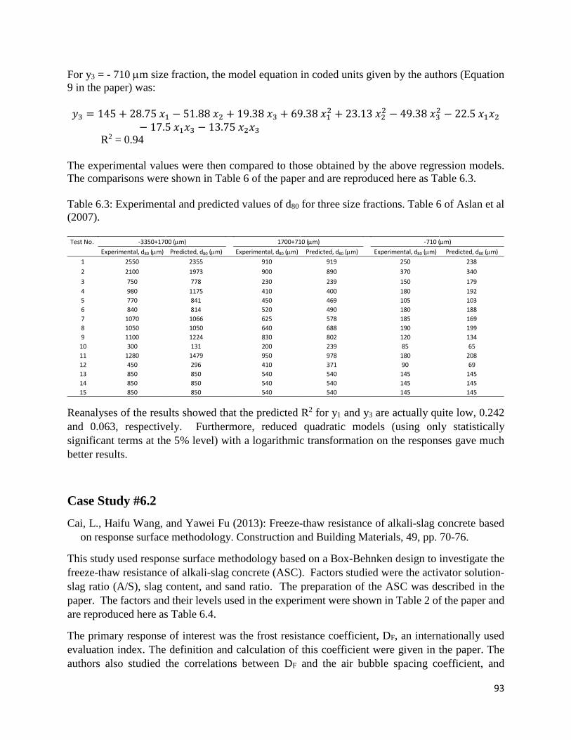
93
For y3 = - 710 µm size fraction, the model equation in coded units given by the authors (Equation 9 in the paper) was: 𝑦𝑦3 = 145 + 28.75 𝑥𝑥1 − 51.88 𝑥𝑥2 + 19.38 𝑥𝑥3 + 69.38 𝑥𝑥12 + 23.13 𝑥𝑥22 − 49.38 𝑥𝑥32 − 22.5 𝑥𝑥1𝑥𝑥2
− 17.5 𝑥𝑥1𝑥𝑥3 − 13.75 𝑥𝑥2𝑥𝑥3 R2 = 0.94
The experimental values were then compared to those obtained by the above regression models. The comparisons were shown in Table 6 of the paper and are reproduced here as Table 6.3. Table 6.3: Experimental and predicted values of d80 for three size fractions. Table 6 of Aslan et al (2007).
Reanalyses of the results showed that the predicted R2 for y1 and y3 are actually quite low, 0.242 and 0.063, respectively. Furthermore, reduced quadratic models (using only statistically significant terms at the 5% level) with a logarithmic transformation on the responses gave much better results.
Case Study #6.2
Cai, L., Haifu Wang, and Yawei Fu (2013): Freeze-thaw resistance of alkali-slag concrete based on response surface methodology. Construction and Building Materials, 49, pp. 70-76.
This study used response surface methodology based on a Box-Behnken design to investigate the freeze-thaw resistance of alkali-slag concrete (ASC). Factors studied were the activator solution-slag ratio (A/S), slag content, and sand ratio. The preparation of the ASC was described in the paper. The factors and their levels used in the experiment were shown in Table 2 of the paper and are reproduced here as Table 6.4.
The primary response of interest was the frost resistance coefficient, DF, an internationally used evaluation index. The definition and calculation of this coefficient were given in the paper. The authors also studied the correlations between DF and the air bubble spacing coefficient, and
Test No. Experimental, d80 (µm) Predicted, d80 (µm) Experimental, d80 (µm) Predicted, d80 (µm) Experimental, d80 (µm) Predicted, d80 (µm)
1 2550 2355 910 919 250 2382 2100 1973 900 890 370 3403 750 778 230 239 150 1794 980 1175 410 400 180 1925 770 841 450 469 105 1036 840 814 520 490 180 1887 1070 1066 625 578 185 1698 1050 1050 640 688 190 1999 1100 1224 830 802 120 13410 300 131 200 239 85 6511 1280 1479 950 978 180 20812 450 296 410 371 90 6913 850 850 540 540 145 14514 850 850 540 540 145 14515 850 850 540 540 145 145
-3350+1700 (µm) 1700+710 (µm) -710 (µm)
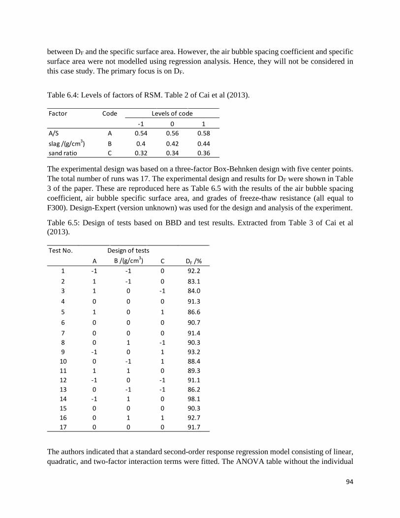
94
between DF and the specific surface area. However, the air bubble spacing coefficient and specific surface area were not modelled using regression analysis. Hence, they will not be considered in this case study. The primary focus is on DF.
Table 6.4: Levels of factors of RSM. Table 2 of Cai et al (2013).
The experimental design was based on a three-factor Box-Behnken design with five center points. The total number of runs was 17. The experimental design and results for DF were shown in Table 3 of the paper. These are reproduced here as Table 6.5 with the results of the air bubble spacing coefficient, air bubble specific surface area, and grades of freeze-thaw resistance (all equal to F300). Design-Expert (version unknown) was used for the design and analysis of the experiment.
Table 6.5: Design of tests based on BBD and test results. Extracted from Table 3 of Cai et al (2013).
The authors indicated that a standard second-order response regression model consisting of linear, quadratic, and two-factor interaction terms were fitted. The ANOVA table without the individual
Factor Code-1 0 1
A/S A 0.54 0.56 0.58slag /(g/cm3) B 0.4 0.42 0.44sand ratio C 0.32 0.34 0.36
Levels of code
Test No.A B /(g/cm3) C DF /%
1 -1 -1 0 92.22 1 -1 0 83.13 1 0 -1 84.04 0 0 0 91.35 1 0 1 86.66 0 0 0 90.77 0 0 0 91.48 0 1 -1 90.39 -1 0 1 93.210 0 -1 1 88.411 1 1 0 89.312 -1 0 -1 91.113 0 -1 -1 86.214 -1 1 0 98.115 0 0 0 90.316 0 1 1 92.717 0 0 0 91.7
Design of tests

95
model terms was shown in Table 4 of the paper and is reproduced here as Table 6.6. The significance tests of the regression coefficients were shown in Table 5 of the paper and are reproduced here as Table 6.7.
Table 6.6: Variance analysis of the model. Table 4 of Cai et al (2013).
Table 6.7: Significance test of the regression coefficients. Table 5 of Cai et al (2013).
Note that the authors did not include the two-factor interactions of AC and BC in the model and they added the A2B term, which is not typical in response surface modelling. No explanation was given for the choice of model. Furthermore, the responses seem to have been multiplied by 10 before analysis. The regression model for DF given by the authors (Equation 3) was:
DF = 910.80 – 39.5A + 21.00B + 11.63C + 0.75AB – 5.40A2 + 1.35B2 – 18.15C2 + 9.25A2B
More accurately, the above equation is for 10DF. The adjusted R2 was 0.9659. No other goodness-of-fit statistics were given. From Table 6.7, many of the model terms are not statistically significant at the 5% level. A reduced model using only statistically significant terms would have given a better model.
Source Sum squares df Mean square F-value p-valueModel 20547.21 8 2568.40 57.61 <0.0001Residual error 356.67 8 44.58Lack of fit 227.87 4 56.97 1.77Pure error 128.80 4 32.20Total 20903.88 16
Term Regression coefficient Std Dev. Lower C.I. of 95% Upper C.I. of 95% P-valueA -39.5 2.36 -44.94 -34.06 <0.0001B 21 3.34 13.30 28.70 0.0002C 11.63 2.36 6.18 17.07 0.0012AB 0.75 3.34 -6.95 8.45 0.8279A2 -5.4 3.25 -12.90 2.10 0.1356B2 1.35 3.25 -6.15 8.85 0.6891C3 -18.15 3.25 -25.65 -10.65 0.0005A2B 9.25 4.72 -1.64 20.14 0.0858
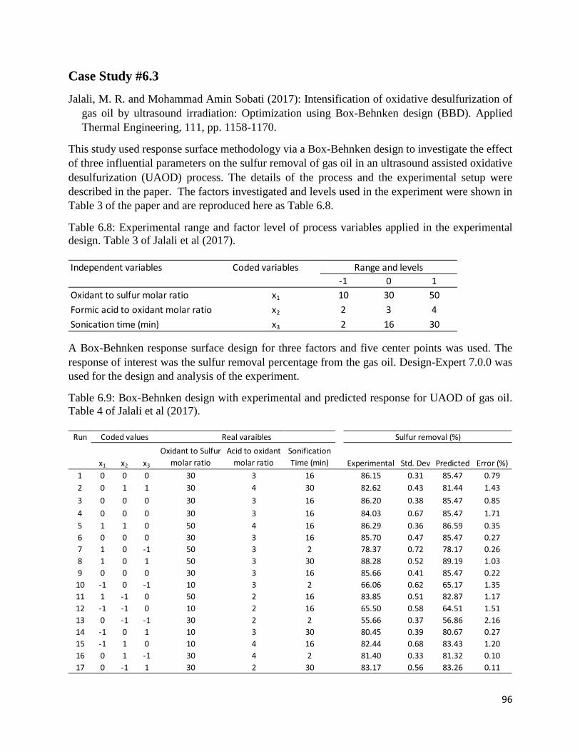
96
Case Study #6.3
Jalali, M. R. and Mohammad Amin Sobati (2017): Intensification of oxidative desulfurization of gas oil by ultrasound irradiation: Optimization using Box-Behnken design (BBD). Applied Thermal Engineering, 111, pp. 1158-1170.
This study used response surface methodology via a Box-Behnken design to investigate the effect of three influential parameters on the sulfur removal of gas oil in an ultrasound assisted oxidative desulfurization (UAOD) process. The details of the process and the experimental setup were described in the paper. The factors investigated and levels used in the experiment were shown in Table 3 of the paper and are reproduced here as Table 6.8.
Table 6.8: Experimental range and factor level of process variables applied in the experimental design. Table 3 of Jalali et al (2017).
A Box-Behnken response surface design for three factors and five center points was used. The response of interest was the sulfur removal percentage from the gas oil. Design-Expert 7.0.0 was used for the design and analysis of the experiment.
Table 6.9: Box-Behnken design with experimental and predicted response for UAOD of gas oil. Table 4 of Jalali et al (2017).
Independent variables Coded variables-1 0 1
Oxidant to sulfur molar ratio x1 10 30 50Formic acid to oxidant molar ratio x2 2 3 4Sonication time (min) x3 2 16 30
Range and levels
Run
x1 x2 x3
Oxidant to Sulfur molar ratio
Acid to oxidant molar ratio
Sonification Time (min) Experimental Std. Dev Predicted Error (%)
1 0 0 0 30 3 16 86.15 0.31 85.47 0.792 0 1 1 30 4 30 82.62 0.43 81.44 1.433 0 0 0 30 3 16 86.20 0.38 85.47 0.854 0 0 0 30 3 16 84.03 0.67 85.47 1.715 1 1 0 50 4 16 86.29 0.36 86.59 0.356 0 0 0 30 3 16 85.70 0.47 85.47 0.277 1 0 -1 50 3 2 78.37 0.72 78.17 0.268 1 0 1 50 3 30 88.28 0.52 89.19 1.039 0 0 0 30 3 16 85.66 0.41 85.47 0.2210 -1 0 -1 10 3 2 66.06 0.62 65.17 1.3511 1 -1 0 50 2 16 83.85 0.51 82.87 1.1712 -1 -1 0 10 2 16 65.50 0.58 64.51 1.5113 0 -1 -1 30 2 2 55.66 0.37 56.86 2.1614 -1 0 1 10 3 30 80.45 0.39 80.67 0.2715 -1 1 0 10 4 16 82.44 0.68 83.43 1.2016 0 1 -1 30 4 2 81.40 0.33 81.32 0.1017 0 -1 1 30 2 30 83.17 0.56 83.26 0.11
Coded values Sulfur removal (%)Real varaibles
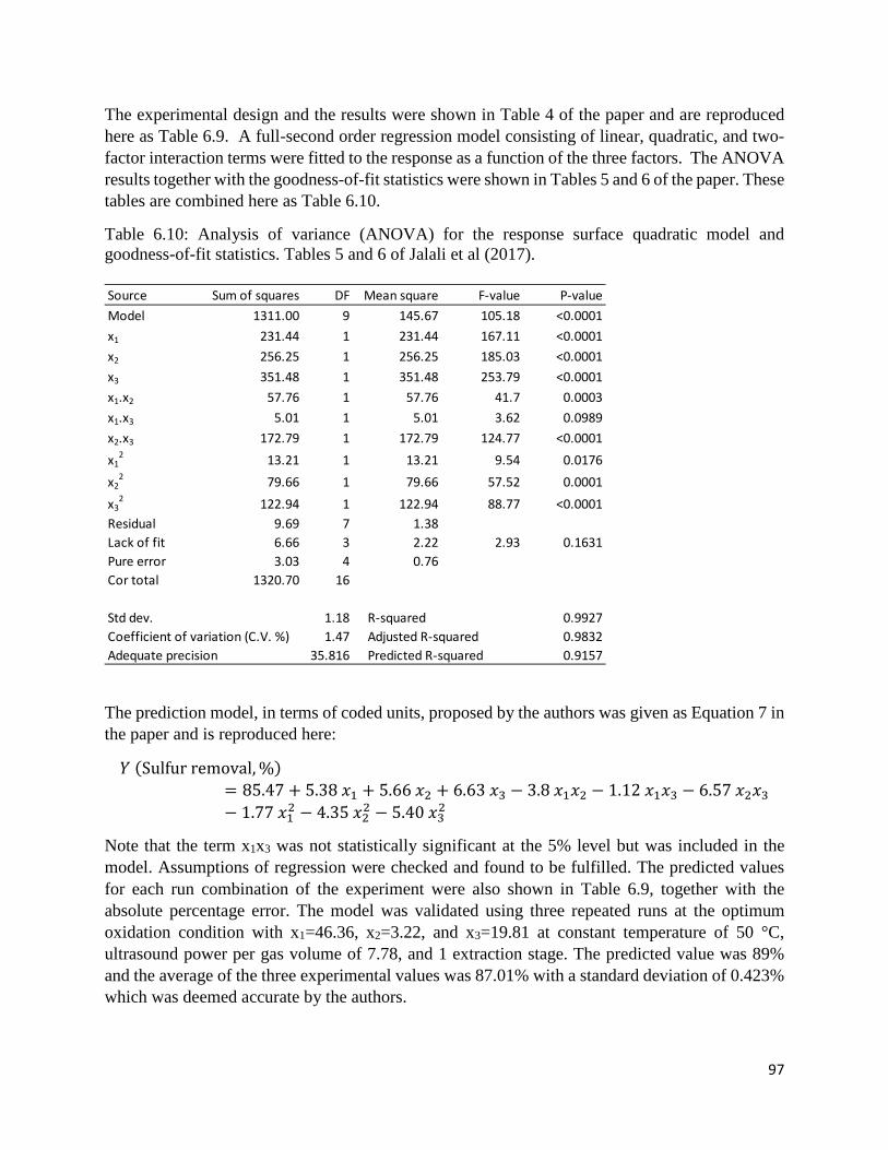
97
The experimental design and the results were shown in Table 4 of the paper and are reproduced here as Table 6.9. A full-second order regression model consisting of linear, quadratic, and two-factor interaction terms were fitted to the response as a function of the three factors. The ANOVA results together with the goodness-of-fit statistics were shown in Tables 5 and 6 of the paper. These tables are combined here as Table 6.10.
Table 6.10: Analysis of variance (ANOVA) for the response surface quadratic model and goodness-of-fit statistics. Tables 5 and 6 of Jalali et al (2017).
The prediction model, in terms of coded units, proposed by the authors was given as Equation 7 in the paper and is reproduced here:
𝑌𝑌 (Sulfur removal, %)= 85.47 + 5.38 𝑥𝑥1 + 5.66 𝑥𝑥2 + 6.63 𝑥𝑥3 − 3.8 𝑥𝑥1𝑥𝑥2 − 1.12 𝑥𝑥1𝑥𝑥3 − 6.57 𝑥𝑥2𝑥𝑥3− 1.77 𝑥𝑥12 − 4.35 𝑥𝑥22 − 5.40 𝑥𝑥32
Note that the term x1x3 was not statistically significant at the 5% level but was included in the model. Assumptions of regression were checked and found to be fulfilled. The predicted values for each run combination of the experiment were also shown in Table 6.9, together with the absolute percentage error. The model was validated using three repeated runs at the optimum oxidation condition with x1=46.36, x2=3.22, and x3=19.81 at constant temperature of 50 °C, ultrasound power per gas volume of 7.78, and 1 extraction stage. The predicted value was 89% and the average of the three experimental values was 87.01% with a standard deviation of 0.423% which was deemed accurate by the authors.
Source Sum of squares DF Mean square F-value P-valueModel 1311.00 9 145.67 105.18 <0.0001x1 231.44 1 231.44 167.11 <0.0001x2 256.25 1 256.25 185.03 <0.0001x3 351.48 1 351.48 253.79 <0.0001x1.x2 57.76 1 57.76 41.7 0.0003x1.x3 5.01 1 5.01 3.62 0.0989x2.x3 172.79 1 172.79 124.77 <0.0001x1
2 13.21 1 13.21 9.54 0.0176x2
2 79.66 1 79.66 57.52 0.0001x3
2 122.94 1 122.94 88.77 <0.0001Residual 9.69 7 1.38Lack of fit 6.66 3 2.22 2.93 0.1631Pure error 3.03 4 0.76Cor total 1320.70 16
Std dev. 1.18 R-squared 0.9927Coefficient of variation (C.V. %) 1.47 Adjusted R-squared 0.9832Adequate precision 35.816 Predicted R-squared 0.9157

98
Case Study #6.4
Kilickap, E. and Mesut Huseyinoglu (2010): Selection of optimum parameters on burr height using response surface methodology and genetic algorithm in drilling of AISI 304 stainless steel. Materials and Manufacturing Processes, 25, pp. 1068-1076.
This study investigated the optimum parameters on burr height using two methodologies. One was based on response surface methodology and another on genetic algorithm. This case study will only consider the method based on response surface methodology via a three-factor Box-Behnken design. The influence of cutting parameters – cutting speed, feed rate, and the point angle was investigated. The response was the burr height. The burr height is an important consideration in drilling of mechanical components. This study used a SX XHMT vertical drilling machine and AISI 304 stainless steel for the drilling experiments. The factors and levels used in the experiment were shown in Table 5 of the paper and are reproduced here as Table 6.11.
Table 6.11: Experimental factors and their levels. Table 5 of Kilickap et al (2010).
The three-factor Box-Behnken design consisted of 12 runs and five center points. The design and the resulting burr heights were shown in Table 6 of the paper. The table is reproduced here as Table 6.12. Design-Expert 6.0 was used for the design and analysis of the experiment.
Table 6.12: Design matrix and observed values of butt height. Table 6 of Kilickap et al (2010).
Symbol Drilling parameter Level 1 (-1) Level 2 (0) Level 3 (+1)A Cutting speed, V (m/min) 4 8 12B Feed rate, f (mm/rev) 0.1 0.2 0.3C Point angle, Ɵ (°) 90 (1) 118 (2) 135 (3)
Trial No. Cutting speed Feed rate Point angle Burr height (mm)1 -1 -1 0 0.722 1 -1 0 1.403 -1 1 0 1.244 1 1 0 2.085 -1 0 -1 1.256 1 0 -1 2.107 -1 0 1 0.828 1 0 1 1.459 0 -1 -1 0.9910 0 1 -1 1.8011 0 -1 1 0.7412 0 1 1 1.4213 0 0 0 1.4414 0 0 0 1.4415 0 0 0 1.4416 0 0 0 1.4417 0 0 0 1.44

99
A quadratic model was suggested by the software. The ANOVA results for the quadratic model were shown in Table 8 of the paper, together with the goodness-of-fit statistics. This table is reproduced here as Table 6.13. No attempt was made by the authors to reduce the model.
Table 6.13: ANOVA table for response surface quadratic model. Table 8 of Kilickap et al (2010).
The prediction equation in actual factors for the burr height (H) was given as (Equation 5 in the paper):
H (mm) = -0.38 + 0.0575 A + 8.1625 B + 0.27625 C + 2.7343 E-03 A2 – 12.375 B2 – 0.07875 C2 + 0.10 AB – 0.01375 AC – 0.325 BC. Note that the levels for the point angle (factor C) must be entered as 1, 2, and 3, and not as the actual angles given in Table 6.11. Five of the regression coefficients were actually statistically insignificant at the 5% level. These terms could have been removed for a better model. The authors concluded that to achieve minimum burr height, a combination of low cutting speed and low feed rate with a larger point angle must be used in the drilling process.
Source Sum of Squares df Mean Square F-value p-valueModel 2.52 9 0.28 54.35 < 0.0001 significantA-A 1.13 1 1.13 218.6 < 0.0001B-B 0.90 1 0.90 175.76 < 0.0001C-C 0.37 1 0.37 71.02 < 0.0001A² 8.059E-03 1 8.059E-03 1.57 0.2510B² 0.064 1 0.064 12.53 0.0095C² 0.026 1 0.026 5.07 0.0590AB 6.40E-03 1 6.400E-03 1.24 0.3016AC 0.012 1 0.012 2.35 0.1691BC 4.225E-03 1 4.225E-03 0.821 0.3950Residual 0.036 7Cor Total 2.55 16S.D. 0.072 C.V. 5.25 R2 0.9859 Pred. R2 0.7743Mean 1.37 PRESS 0.58 Adj. R2 0.9678 Adeq. Precision 25.854
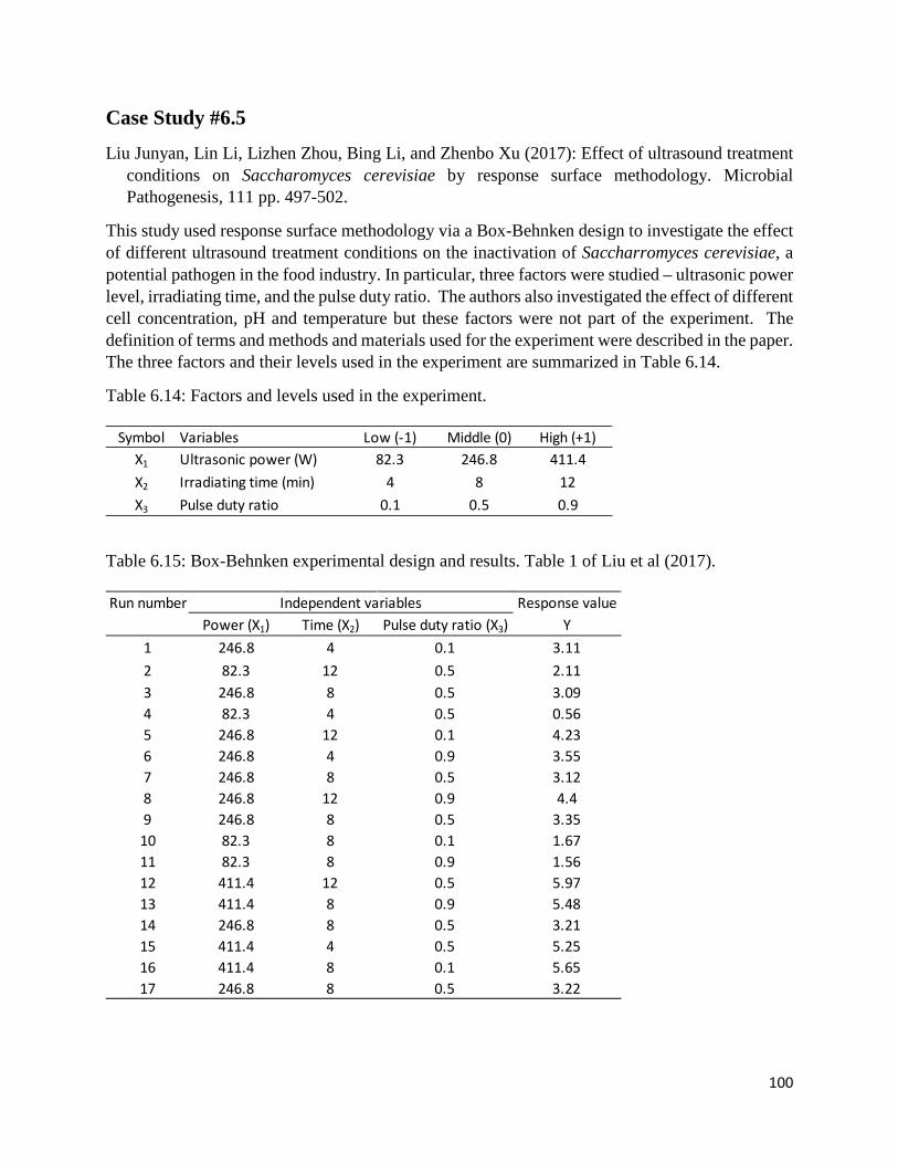
100
Case Study #6.5
Liu Junyan, Lin Li, Lizhen Zhou, Bing Li, and Zhenbo Xu (2017): Effect of ultrasound treatment conditions on Saccharomyces cerevisiae by response surface methodology. Microbial Pathogenesis, 111 pp. 497-502.
This study used response surface methodology via a Box-Behnken design to investigate the effect of different ultrasound treatment conditions on the inactivation of Saccharromyces cerevisiae, a potential pathogen in the food industry. In particular, three factors were studied – ultrasonic power level, irradiating time, and the pulse duty ratio. The authors also investigated the effect of different cell concentration, pH and temperature but these factors were not part of the experiment. The definition of terms and methods and materials used for the experiment were described in the paper. The three factors and their levels used in the experiment are summarized in Table 6.14.
Table 6.14: Factors and levels used in the experiment.
Table 6.15: Box-Behnken experimental design and results. Table 1 of Liu et al (2017).
Symbol Variables Low (-1) Middle (0) High (+1)X1 Ultrasonic power (W) 82.3 246.8 411.4X2 Irradiating time (min) 4 8 12X3 Pulse duty ratio 0.1 0.5 0.9
Run number Response valuePower (X1) Time (X2) Pulse duty ratio (X3) Y
1 246.8 4 0.1 3.112 82.3 12 0.5 2.113 246.8 8 0.5 3.094 82.3 4 0.5 0.565 246.8 12 0.1 4.236 246.8 4 0.9 3.557 246.8 8 0.5 3.128 246.8 12 0.9 4.49 246.8 8 0.5 3.3510 82.3 8 0.1 1.6711 82.3 8 0.9 1.5612 411.4 12 0.5 5.9713 411.4 8 0.9 5.4814 246.8 8 0.5 3.2115 411.4 4 0.5 5.2516 411.4 8 0.1 5.6517 246.8 8 0.5 3.22
Independent variables

101
A three-factor Box-Behnken design with five center points (total of 17 points) was used for the experiment. Design-Expert 7.0 was used for the design and subsequent analysis of the results. The response was based on a plate counting method to identify ultrasound treatment efficiency. The response Y was expressed as –lg(N/N0), where, N0 is the initial cell number and N is the cell number in the sample after different treatments. The average of at least three plates was used as the response. The experimental design and the results were shown in Table 1 of the paper and are reproduced here as Table 6.15.
The authors fitted a standard second-order response surface model with linear, quadratic, and two-factor interaction terms to the response. The ANOVA results were shown in Table 2 of the paper. The table is reproduced here as Table 6.16.
Table 6.16: ANOVA results for the response surface model. Table 2 of Liu et al (2017).
The prediction equation was given as Equation 2 in the paper as: 𝑌𝑌 = 3.20 + 2.06𝑋𝑋1 + 0.53𝑋𝑋2 + 0.041𝑋𝑋3 − 0.21𝑋𝑋1𝑋𝑋2 − 0.015𝑋𝑋1𝑋𝑋3 − 0.068 𝑋𝑋2𝑋𝑋3 − 0.021𝑋𝑋12
+ 0.25𝑋𝑋22 + 0.37𝑋𝑋32 Note that the prediction equation included all terms regardless of their statistical significance. A reduced quadratic model with only statistically significant terms at the 5% level would have provided a higher predicted R2.
The authors concluded that ultrasound power played the most important role in the irradiation process of Saccharromyces cerevisiae during ultrasound treatment in the food industry.
Source Sum of Squares df Mean Square F-value p-valueModel 37.18 9 4.13 141.38 < 0.0001 significantX1 33.83 1 33.83 1157.44 < 0.0001X2 2.25 1 2.25 76.89 < 0.0001X3 0.014 1 0.014 0.47 0.5169X1X2 0.17 1 0.17 5.89 0.0456X1X3 9.00E-04 1 9.00E-04 0.031 0.8657X2X3 0.018 1 0.018 0.62 0.4556X1² 1.857E-03 1 1.857E-03 0.064 0.8082X2² 0.27 1 0.27 9.26 0.0188X3² 0.58 1 0.58 19.83 0.0030Residual 0.20 7 0.029Lack of Fit 0.16 3 0.054 5.24 0.0717 not significantPure Error 0.042 4 0.010Cor Total 37.39 16R-squared 0.9945 Predicted R-squared 0.9285Adjusted R-square 0.9875

102
Case Study #6.6
Muthukumar, M., D. Mohan, and M. Rajendran (2003): Optimization of mix proportions of mineral aggregates using Box-Behnken design of experiments. Cement and Concrete Composites, 25, pp. 751-758.
This study investigated the optimal mix proportions of silica aggregates for use in polymer concrete using a six-factor Box-Behnken response surface design. The six factors were the six different grades of particle sizes ranging in size from 0.15 to 9.72 mm. The primary objective was to determine what combination of particle sizes would minimize the void content of the resulting concrete. The materials and methods used for the experiment were described in the paper. The factors and levels used in the experiment were shown in Table 1 of the paper and are reproduced here as Table 6.17.
Table 6.17: Levels of variables chose for the design. Table 1 of Muthukumar et al (2003).
The Box-Behnken design with the six factors used 54 run combinations (49 points and six center points). Design-Expert (version unknown) was used for the design and analysis of the experiment. The response was the void content (%). The experimental design together with the results were shown in Table 5 of the paper and are reproduced here as Table 6.18. A second-order polynomial regression was fitted to the experimental results and the ANOVA results were shown in Table 4 of the paper (reproduced here as Table 6.19). The prediction equation (in coded factors) for the void content was the full second-order polynomial equation given in the paper as: Predicted void content (%) = 24.81 - 1.986x1 - 1.147x2 - 0.132x3 + 1.210x4 + 1.088x5 - 0.520x6 + 0.602x1
2 + 0.571x22 + 0.239x3
2 + 0.192x42 + 0.684x5
2+ 1.401x62 + 1.155x1x2 + 0.443x1x3
+ 0.032x1x4 - 0.791x1x5 - 0.12x1x6 + 0.899x2x3 + 0.030x2x4 - 0.712x2x5 - 0.609x2x6 - 0.375x3x4 - 0.981x3x5 - 0.939x3x6 - 0.281x4x5 - 0.580x4x6 + 1.336x5x6 (R2 = 0.9174) As can be seen from the ANOVA table, more than 10 of the regression coefficients were actually not statistically significant at the 5% level yet they were included in the prediction equation. The only goodness-of-fit statistic given was the R2 value of 0.9174. The adjusted and predicted R2 were not reported. The comparison of the experimental and predicted values were also shown in Table 6.18.
S. no. GradeMin Max Low Medium High
1 A 4.76 9.52 0 (-1) 50 (0) 100 (+1)2 B 2.38 4.76 0 (-1) 50 (0) 100 (+1)3 C 1.19 2.38 0 (-1) 50 (0) 100 (+1)4 D 0.60 1.19 0 (-1) 50 (0) 100 (+1)5 E 0.30 0.60 0 (-1) 50 (0) 100 (+1)6 F 0.15 0.30 0 (-1) 50 (0) 100 (+1)
Particle size, mm Input level, g (coded)

103
Table 6.18: Box Behnken design for the six variables and their experimental and predicted response (% void content). Table 5 of Muthukumar et al (2003).
Run A B C D E F Experimental response Predicted response1 -1 -1 0 -1 0 0 30.16 29.322 0 -1 -1 0 -1 0 25.46 25.703 0 1 0 0 1 1 26.37 26.904 0 0 -1 1 0 1 27.83 28.205 0 0 -1 -1 0 1 27.62 26.196 1 0 0 1 -1 0 24.96 25.537 -1 -1 0 1 0 0 31.28 31.618 -1 0 1 0 0 1 27.37 27.139 1 0 0 1 1 0 26.12 25.5610 1 0 -1 0 0 1 24.87 25.0611 0 0 1 -1 0 -1 27.25 26.5512 -1 0 -1 0 0 -1 29.41 29.0713 0 -1 0 0 1 -1 29.53 28.9914 -1 0 0 1 -1 0 28.08 27.8515 1 -1 0 -1 0 0 21.96 22.9716 1 0 0 -1 -1 0 23.83 22.4817 -1 0 -1 0 0 1 30.66 30.1518 0 0 1 1 0 -1 28.28 29.3819 0 -1 1 0 1 0 27.91 27.2420 0 -1 0 0 -1 -1 28.28 28.0621 1 0 1 0 0 1 23.79 23.8022 -1 0 0 1 1 0 30.12 31.0523 0 1 1 0 1 0 25.87 25.3224 -1 1 0 1 0 0 27.66 27.0725 0 -1 0 0 1 1 30.28 31.8426 0 1 0 0 -1 -1 30.28 28.4127 0 0 0 0 0 0 25.25 24.8128 -1 0 0 -1 -1 0 23.96 24.9429 1 1 0 -1 0 0 22.84 22.9330 0 0 0 0 0 0 24.33 24.8131 0 -1 0 0 -1 1 25.62 25.5732 0 1 0 0 -1 1 23.25 23.4833 0 -1 1 0 -1 0 25.33 25.6034 -1 0 0 -1 1 0 29.41 29.2635 0 0 1 -1 0 1 24.25 24.8036 0 1 1 0 -1 0 26.08 26.5337 0 0 0 0 0 0 24.83 24.8138 1 0 0 -1 1 0 23.83 23.6439 0 0 0 0 0 0 25.33 24.8140 0 0 1 1 0 1 26.50 25.3141 0 1 -1 0 -1 0 22.05 23.0342 -1 1 0 -1 0 0 24.13 24.6543 0 -1 -1 0 1 0 31.40 31.2644 0 0 -1 1 0 -1 28.74 28.5245 -1 0 1 0 0 -1 29.66 29.8046 1 0 -1 0 0 -1 24.54 24.4647 0 0 -1 -1 0 -1 22.67 24.1948 0 1 -1 0 1 0 26.33 25.7549 1 0 1 0 0 -1 26.12 26.9650 0 1 0 0 1 -1 26.12 26.4951 0 0 0 0 0 0 24.50 24.8152 1 -1 0 1 0 0 26.33 25.3953 0 0 0 0 0 0 24.62 24.8154 1 1 0 1 0 0 25.04 25.47

104
Table 6.19: ANOVA for response surface quadratic model. Table 4 of Muthukumar et al (2003).
From Table 6.19, it can be seen that the lack of fit of the fitted model was statistically significant at 5% level. This lack of fit was not addressed in the paper. If a reduced quadratic model was fitted with only statistically significant terms, the predicted R2 would have increased from 0.578 to 0.726.
The authors then obtained the optimal combination to give the minimum void content. This was compared to the minimum void content obtained from the 54 experiments. This comparison was shown in Table 6 of the paper and is shown here as Table 6.20.
Source Sum of Squares DF Mean Square F-value p-valueModel 300.71 27 11.140 10.699 < 0.0001x1 94.68 1 94.685 90.956 < 0.0001x2 31.56 1 31.556 30.313 < 0.0001x3 0.42 1 0.419 0.402 0.5315x4 35.11 1 35.114 33.731 < 0.0001x5 28.41 1 28.406 27.287 < 0.0001x6 6.48 1 6.479 6.224 0.0193x1² 3.73 1 3.730 3.583 0.0695x2² 3.35 1 3.348 3.216 0.0845x3² 0.59 1 0.587 0.564 0.4594x4² 0.38 1 0.380 0.365 0.5509x5² 4.82 1 4.817 4.627 0.0409x6² 20.20 1 20.200 19.404 0.0002x1.x2 10.67 1 10.672 10.252 0.0036x1.x3 1.57 1 1.566 1.505 0.2309x1x4 0.02 1 0.016 0.016 0.9015x1x5 5.01 1 5.009 4.811 0.0374x1x6 0.12 1 0.115 0.111 0.7421x2x3 6.46 1 6.462 6.208 0.0194x2x4 0.01 1 0.007 0.007 0.9344x2x5 8.12 1 8.123 7.803 0.0097x2x6 2.96 1 2.965 2.848 0.1035x3x4 1.13 1 1.125 1.081 0.3081x3x5 7.70 1 7.703 7.399 0.0115x3x6 14.10 1 14.100 13.545 0.0011x4x5 0.63 1 0.633 0.608 0.4426x4x6 2.69 1 2.691 2.585 0.1199x5x6 14.28 1 14.285 13.722 0.0010
Residual 27.07 26 1.041Lack of Fit 26.24 21 1.249 7.554 0.0169Pure Error 0.83 5 0.165Cor Total 327.78 53
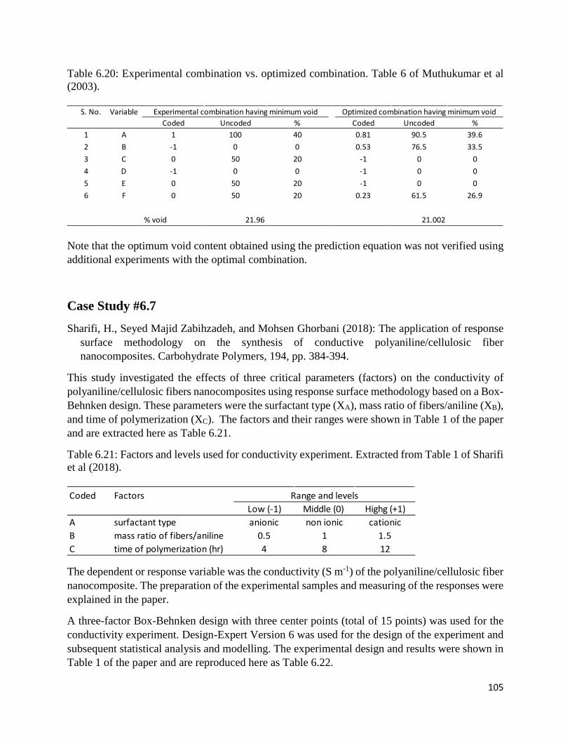
105
Table 6.20: Experimental combination vs. optimized combination. Table 6 of Muthukumar et al (2003).
Note that the optimum void content obtained using the prediction equation was not verified using additional experiments with the optimal combination.
Case Study #6.7
Sharifi, H., Seyed Majid Zabihzadeh, and Mohsen Ghorbani (2018): The application of response surface methodology on the synthesis of conductive polyaniline/cellulosic fiber nanocomposites. Carbohydrate Polymers, 194, pp. 384-394.
This study investigated the effects of three critical parameters (factors) on the conductivity of polyaniline/cellulosic fibers nanocomposites using response surface methodology based on a Box-Behnken design. These parameters were the surfactant type (XA), mass ratio of fibers/aniline (XB), and time of polymerization (XC). The factors and their ranges were shown in Table 1 of the paper and are extracted here as Table 6.21.
Table 6.21: Factors and levels used for conductivity experiment. Extracted from Table 1 of Sharifi et al (2018).
The dependent or response variable was the conductivity (S m-1) of the polyaniline/cellulosic fiber nanocomposite. The preparation of the experimental samples and measuring of the responses were explained in the paper.
A three-factor Box-Behnken design with three center points (total of 15 points) was used for the conductivity experiment. Design-Expert Version 6 was used for the design of the experiment and subsequent statistical analysis and modelling. The experimental design and results were shown in Table 1 of the paper and are reproduced here as Table 6.22.
S. No. VariableCoded Uncoded % Coded Uncoded %
1 A 1 100 40 0.81 90.5 39.62 B -1 0 0 0.53 76.5 33.53 C 0 50 20 -1 0 04 D -1 0 0 -1 0 05 E 0 50 20 -1 0 06 F 0 50 20 0.23 61.5 26.9
% void 21.96 21.002
Experimental combination having minimum void Optimized combination having minimum void
Coded FactorsLow (-1) Middle (0) Highg (+1)
A surfactant type anionic non ionic cationicB mass ratio of fibers/aniline 0.5 1 1.5C time of polymerization (hr) 4 8 12
Range and levels
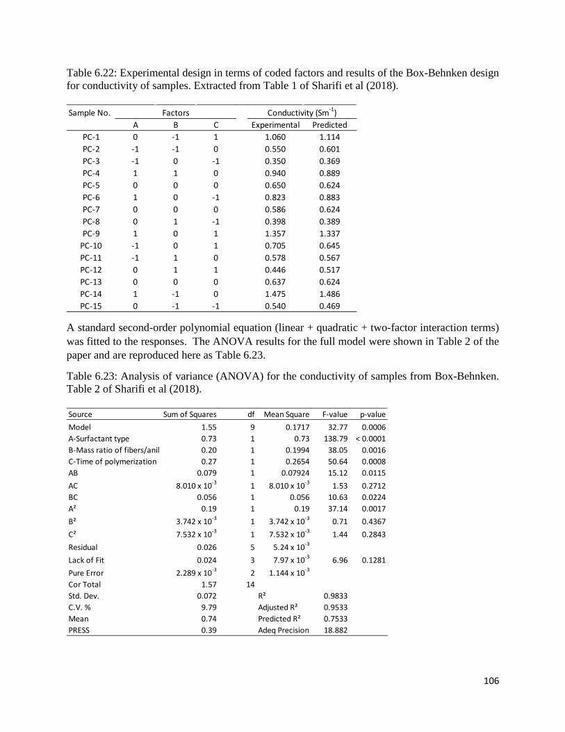
106
Table 6.22: Experimental design in terms of coded factors and results of the Box-Behnken design for conductivity of samples. Extracted from Table 1 of Sharifi et al (2018).
A standard second-order polynomial equation (linear + quadratic + two-factor interaction terms) was fitted to the responses. The ANOVA results for the full model were shown in Table 2 of the paper and are reproduced here as Table 6.23.
Table 6.23: Analysis of variance (ANOVA) for the conductivity of samples from Box-Behnken. Table 2 of Sharifi et al (2018).
Sample No.A B C Experimental Predicted
PC-1 0 -1 1 1.060 1.114PC-2 -1 -1 0 0.550 0.601PC-3 -1 0 -1 0.350 0.369PC-4 1 1 0 0.940 0.889PC-5 0 0 0 0.650 0.624PC-6 1 0 -1 0.823 0.883PC-7 0 0 0 0.586 0.624PC-8 0 1 -1 0.398 0.389PC-9 1 0 1 1.357 1.337
PC-10 -1 0 1 0.705 0.645PC-11 -1 1 0 0.578 0.567PC-12 0 1 1 0.446 0.517PC-13 0 0 0 0.637 0.624PC-14 1 -1 0 1.475 1.486PC-15 0 -1 -1 0.540 0.469
Conductivity (Sm-1)Factors
Source Sum of Squares df Mean Square F-value p-valueModel 1.55 9 0.1717 32.77 0.0006A-Surfactant type 0.73 1 0.73 138.79 < 0.0001B-Mass ratio of fibers/anil 0.20 1 0.1994 38.05 0.0016C-Time of polymerization 0.27 1 0.2654 50.64 0.0008AB 0.079 1 0.07924 15.12 0.0115AC 8.010 x 10⁻³ 1 8.010 x 10⁻³ 1.53 0.2712BC 0.056 1 0.056 10.63 0.0224A² 0.19 1 0.19 37.14 0.0017B² 3.742 x 10⁻³ 1 3.742 x 10⁻³ 0.71 0.4367C² 7.532 x 10⁻³ 1 7.532 x 10⁻³ 1.44 0.2843Residual 0.026 5 5.24 x 10⁻³
Lack of Fit 0.024 3 7.97 x 10⁻³ 6.96 0.1281Pure Error 2.289 x 10⁻³ 2 1.144 x 10⁻³
Cor Total 1.57 14Std. Dev. 0.072 R² 0.9833C.V. % 9.79 Adjusted R² 0.9533Mean 0.74 Predicted R² 0.7533PRESS 0.39 Adeq Precision 18.882

107
Based on the ANOVA results for the full model, the authors considered that fitted model was statistically significant and provided a very good fit. Hence, they suggested the following prediction equation in coded factors (Equation 4 in the paper):
Conductivity = 0.62433 + 0.30150 XA - 0.15788 XB + 0.18213 XC + 0.229583 XA
2 + 0.031833 XB
2 - 0.045167 XC2 - 0.14075 XAXB + 0.04475 XAXC - 0.11800 XBXC
The predicted conductivity for the same run combinations are also shown in Table 6.22. Note that several of the coefficients in the prediction model are not statistically significant at the 5% level. The adequacy of the model was checked by the authors and found to be satisfactory. A reduced model using only statistically significant terms would have provided a model with higher predicted R2.
The authors then validated the prediction model using three additional experimental runs - one run for each type of surfactant. The results were shown in Table 3 of the paper are shown here as Table 6.24.
Table 6.24: Comparing the experimental and predicted values. Table 3 of Sharifi et al (2018).
The interpretation of the coefficients and results were given in the paper. The optimum conditions maximizing conductivity were found to be: use of cationic surfactant, mass ratio of fibers/aniline of about 0.5, and time of polymerization of 8 hours. The maximum conductivity obtained was 1.48587 S m-1. The optimization technique used was not described in the paper.
Case Study #6.8
Zhang, H., Yanli Li, and Xiaogang Wu (2012): Statistical experiment design approach for the treatment of landfill leachate by photoelectro-fenton process. ASCE Journal of Environmental Engineering, Vol. 138, No. 3, pp. 278-285.
This study investigated the influence of three different variables – ferrous ion dosage, hydrogen peroxide concentration, and current density on the photoelectro-Fenton process for the treatment of landfill leachate using response surface methodology. A Box-Behnken design was used to develop the prediction models for two responses – color removal and COD removal. According to the authors, among various advanced oxidation processes for landfill leachate treatment, the Fenton process has been widely used due to its simplicity and ease of implementation.
Run no. Surfactant type Mass ratio of fibers/aniline Time of polymerization |Error (%)|Experimenta Predicted
1 cationic 0.7 12 1.468±0.046 1.52152 3.642 anionic 1.1 10 0.643±0.0195 0.59153 1.93 non ionic 1.4 6 0.466±0.064 0.45923 1.45
a Mean ± standard deviation
Conductivity

108
The factors and levels considered in the experiment are shown in Table 6.25. Table 6.25: Factors and levels used in the landfill treatment experiment.
A Box-Behnken design with three center points (total of 15 runs) was used to generate the design points. The two responses measured were: the color removal percentage (Y1) and the COD removal percentage (Y2). The design matrix in coded and uncoded units and the responses were shown in Table 1 of the paper and are reproduced here as Table 6.26. Design-Expert software (version unknown) was used to design and analyze of the experiment.
Table 6.26: Design matrix in coded and uncoded units and the experimental responses. Table 1 of Zhang et al (2012).
The authors then fitted a standard second-order polynomial (linear + quadratic + two-factor interaction terms) to each of the responses. The reduced ANOVA tables for Y1 (color removal percentage) and Y2 (COD removal percentage) were shown as Tables 2 and 3 in the paper. These tables are reproduced here as Tables 6.27 and 6.28, respectively.
Factor Factor name and unitsLow (-1) Middle (0) High (+1)
x1 Ferrous iron dosage (Fe2+), mmol L-1 8.75 29.75 50.75x2 Hydrogen peroxide concentration (H2O2), mmol L-1 87.5 219.0 350.0x3 Current density, mA cm-2 8.33 16.67 25.00
Levels
Std Order
Fe2+ (mmol L-1) (x1)
H2O2 (mmol L-1) (x2)
Current density (mA cm-2) (x3) Observed Predicted Observed Predicted
1 8.75 (-1) 87.5 (-1) 16.67 (0) 83.5 82.4 47.9 48.472 50.75 (+1) 87.5 (-1) 16.67 (0) 79.6 81.2 60.5 63.793 8.75 (-1) 350 (+1) 16.67 (0) 94.2 92.6 61.7 58.44 50.75 (+1) 350 (+1) 16.67 (0) 90.8 91.9 75.8 75.35 8.75 (-1) 219 (0) 8.33 (-1) 84.4 85.5 50.6 50.56 50.75 (+1) 219 (0) 8.33 (-1) 89.4 87.9 71.4 68.57 8.75 (-1) 219 (0) 25 (+1) 91.9 93.4 57.6 60.58 50.75 (+1) 219 (0) 25 (+1) 90.0 88.9 74.6 74.79 29.75 (0) 87.5 (-1) 8.33 (-1) 80.2 80.2 59.1 58.6
10 29.75 (0) 350 (+1) 8.33 (-1) 90.5 90.9 65.1 68.511 29.75 (0) 87.5 (-1) 25 (+1) 85.4 84.9 69.4 66.012 29.75 (0) 350 (+1) 25 (+1) 95.0 95.1 77.0 77.513 29.75 (0) 219 (0) 16.67 (0) 92.4 92.5 73.4 74.114 29.75 (0) 219 (0) 16.67 (0) 91.2 92.5 74.4 74.115 29.75 (0) 219 (0) 16.67 (0) 94.0 92.5 74.4 74.1
Uncoded and coded levels of variables Color removal (%) (Y1) COD removal (%) (Y2)

109
Table 6.27: Test for response function Y1 (color removal in percentage). Table 2 of Zhang et al (2012).
Using the terms in Table 6.27, the authors suggested the following prediction equation (equation 6 in the paper) for Y1:
𝑌𝑌1 = 91.65 + 5.22 𝑋𝑋2 + 2.22 𝑋𝑋3 − 2.08 𝑋𝑋12 − 3.21 𝑋𝑋22
The R2 value for Y1 was 0.8862, and adjusted R2 value was 0.8406. The predicted R2 value was not given. It should be noted that the 𝑋𝑋12 term is not statistically significant at the 5% level and can be left out. If this term is included, then the X1 term should also be included in the model for hierarchy.
Table 6.28: Test for response function Y2 (COD removal in percentage). Table 3 of Zhang et al (2012).
For Y2, the suggested prediction equation was (equation 7 in the paper):
𝑌𝑌2 = 72.75 + 8.07 𝑋𝑋1 + 5.36 𝑋𝑋2 + 4.07 𝑋𝑋3 − 8.18 𝑋𝑋12 − 4.09 𝑋𝑋22
The R2 value for Y2 was 0.9319, and adjusted R2 value was 0.8940. The predicted R2 value was not given. The coefficients of this model were all statistically significant at the 5% level and the model is hierarchical.
Source Sum of Squares df Mean Square F-value p-valueModel 308.53 4 77.13 19.46 0.0001X2 218.09 1 218.09 55.02 < 0.0001X3 39.43 1 39.43 9.95 0.0103X1
2 16.00 1 16.00 4.04 0.0723X2² 38.29 1 38.29 9.66 0.0111Residual 39.64 10 3.96Lack of Fit 35.77 8 4.47 2.31 0.3366Pure Error 3.86 2 1.93Cor Total 348.17 14
Source Sum of Squares df Mean Square F-value p-valueModel 1177.39 5 235.48 24.62 < 0.0001X1 520.40 1 520.40 54.41 < 0.0001X2 229.84 1 229.84 24.03 0.0008X3 132.56 1 132.56 13.86 0.0048X1² 248.77 1 248.77 26.01 0.0006X2² 62.08 1 62.08 6.49 0.0313Residual 86.08 9 9.56Lack of Fit 85.40 7 12.20 35.79 0.0274Pure Error 0.68 2 0.34Cor Total 1259.53 14

110
The assumptions of regression were checked by the authors and found to be satisfactory. The authors concluded that the photoelectron-Fenton process was capable of efficiently removing COD from landfill leachate. The results also showed that there was no interaction effect between the factors studied. The optimal conditions for color removal (of over 90%) and COD removal (of over 75%) were obtained using an overlay plot of the two response functions. One possible solution to achieve the above optimal condition was setting ferrous ion and hydrogen peroxide dosages at 38.99 and 153.2 mmol L-1, respectively at a current density of 25 mA cm-2. The authors did not use the desirable function approach for optimization available in Design-Expert.
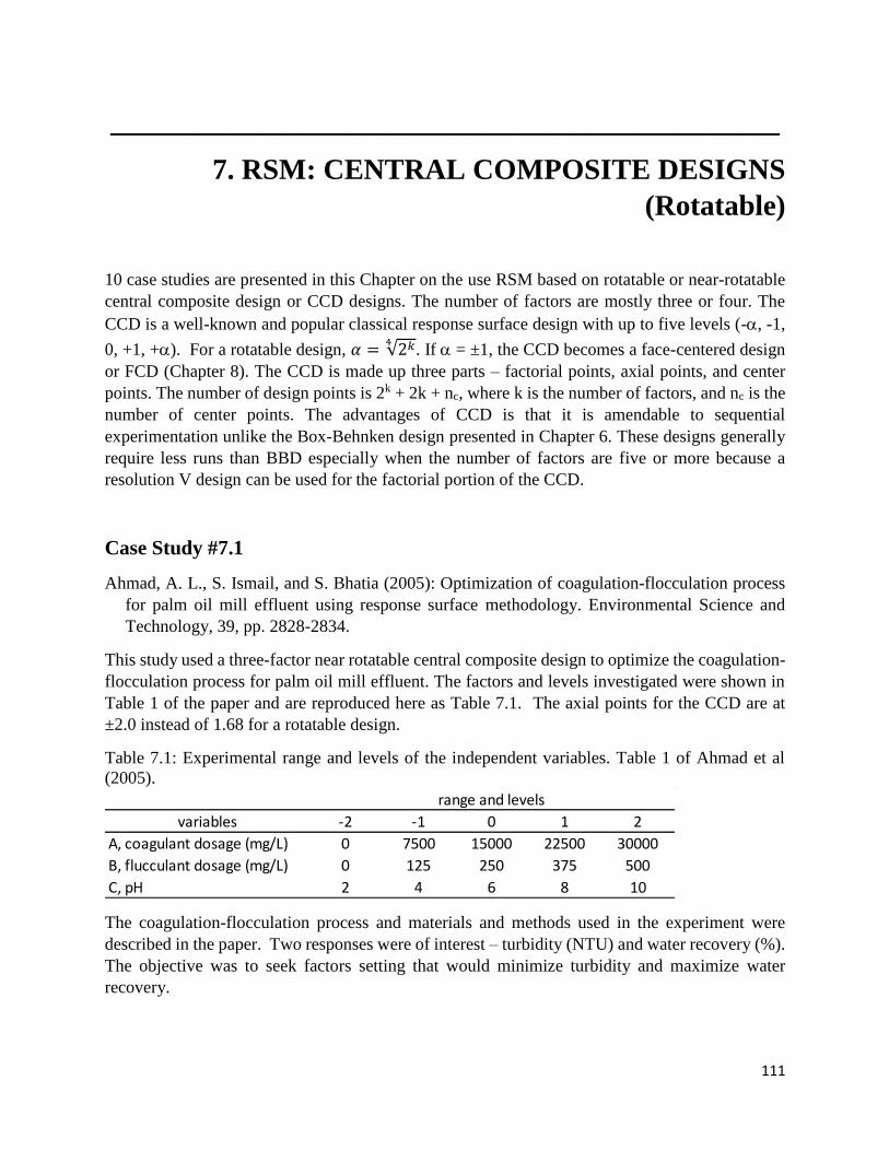
111
______________________________________________
7. RSM: CENTRAL COMPOSITE DESIGNS
(Rotatable)
10 case studies are presented in this Chapter on the use RSM based on rotatable or near-rotatable
central composite design or CCD designs. The number of factors are mostly three or four. The
CCD is a well-known and popular classical response surface design with up to five levels (-, -1,
0, +1, +). For a rotatable design, 𝛼 = √2𝑘4
. If = ±1, the CCD becomes a face-centered design
or FCD (Chapter 8). The CCD is made up three parts – factorial points, axial points, and center
points. The number of design points is 2k + 2k + nc, where k is the number of factors, and nc is the
number of center points. The advantages of CCD is that it is amendable to sequential
experimentation unlike the Box-Behnken design presented in Chapter 6. These designs generally
require less runs than BBD especially when the number of factors are five or more because a
resolution V design can be used for the factorial portion of the CCD.
Case Study #7.1
Ahmad, A. L., S. Ismail, and S. Bhatia (2005): Optimization of coagulation-flocculation process
for palm oil mill effluent using response surface methodology. Environmental Science and
Technology, 39, pp. 2828-2834.
This study used a three-factor near rotatable central composite design to optimize the coagulation-
flocculation process for palm oil mill effluent. The factors and levels investigated were shown in
Table 1 of the paper and are reproduced here as Table 7.1. The axial points for the CCD are at
±2.0 instead of 1.68 for a rotatable design.
Table 7.1: Experimental range and levels of the independent variables. Table 1 of Ahmad et al
(2005).
The coagulation-flocculation process and materials and methods used in the experiment were
described in the paper. Two responses were of interest – turbidity (NTU) and water recovery (%).
The objective was to seek factors setting that would minimize turbidity and maximize water
recovery.
variables -2 -1 0 1 2
A, coagulant dosage (mg/L) 0 7500 15000 22500 30000
B, flucculant dosage (mg/L) 0 125 250 375 500
C, pH 2 4 6 8 10
range and levels

112
The CCD design layout in coded units and the responses were shown in Tables 2 and 3 of the
paper. These tables are combined and reproduced here as Table 7.2. According to the authors, the
CCD was a follow-up design after a 2-level factorial experiment with eight runs and four center
points (runs 1-12). The 2-level design was then augmented with an additional six center points
and two axial points (runs 13-20) giving a total of 20 design points. The additional eight runs were
put in a second block. Hence, the CCD was analyzed as two blocks. Design-Expert 6.0 was used
for the design and analysis of the experiment.
Table 7.2: CCD for the study of three experimental variables in coded units and results. Tables 2
and 3 of Ahmad et al (2005).
A full second-order quadratic model was first fitted to the log base 10 transformations of the
turbidity data. The ANOVA results were shown in Table 4 of the paper and are reproduced here
as Table 7.3. Based on the ANOVA results, the authors concluded that the model was highly
significant with high R2 and adjusted R2 values. They suggested the following regression equation
as the empirical model (in terms of coded factors) for turbidity (Equation 3 in the paper):
Turbidity (log10) = 1.274 – 0.295A – 0.103B – 0.160C + 0.260A2 + 0.164B2 + 0.394C2 – 0.120AB
-0.399AC – 0.146 BC
coagulant dosage flocculant dosage pH turbidity log10 of water
run no. (A) (B) (C) (NTU) turbidity recovery (%)
1 -1 1 -1 230.35 2.3624 68.0
2 1 -1 1 92.14 1.9644 53.0
3 0 0 0 15.19 1.1816 79.8
4 -1 1 1 785.75 2.8953 52.0
5 -1 -1 1 892.40 2.9506 59.0
6 0 0 0 16.10 1.2068 74.8
7 -1 -1 -1 142.50 2.1538 74.0
8 1 1 -1 310.85 2.4926 81.0
9 0 0 0 13.91 1.1433 75.2
10 1 1 1 12.86 1.1092 68.4
11 1 -1 -1 279.15 2.4458 74.0
12 0 0 0 18.53 1.2679 77.2
13 2 0 0 32.57 1.5128 70.8
14 0 0 2 137.75 2.1391 51.0
15 0 0 0 29.53 1.4703 70.2
16 0 0 0 27.10 1.4330 74.0
17 0 -2 0 93.83 1.9723 38.0
18 0 0 -2 1409.25 3.1490 68.0
19 0 2 0 29.86 1.4751 73.6
20 -2 0 0 502.15 2.7008 92.8
factor responses
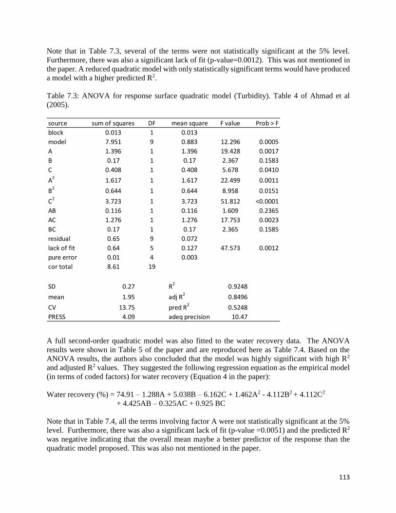
113
Note that in Table 7.3, several of the terms were not statistically significant at the 5% level.
Furthermore, there was also a significant lack of fit (p-value=0.0012). This was not mentioned in
the paper. A reduced quadratic model with only statistically significant terms would have produced
a model with a higher predicted R2.
Table 7.3: ANOVA for response surface quadratic model (Turbidity). Table 4 of Ahmad et al
(2005).
A full second-order quadratic model was also fitted to the water recovery data. The ANOVA
results were shown in Table 5 of the paper and are reproduced here as Table 7.4. Based on the
ANOVA results, the authors also concluded that the model was highly significant with high R2
and adjusted R2 values. They suggested the following regression equation as the empirical model
(in terms of coded factors) for water recovery (Equation 4 in the paper):
Water recovery (%) = 74.91 – 1.288A + 5.038B – 6.162C + 1.462A2 - 4.112B2 + 4.112C2
+ 4.425AB – 0.325AC + 0.925 BC
Note that in Table 7.4, all the terms involving factor A were not statistically significant at the 5%
level. Furthermore, there was also a significant lack of fit (p-value =0.0051) and the predicted R2
was negative indicating that the overall mean maybe a better predictor of the response than the
quadratic model proposed. This was also not mentioned in the paper.
source sum of squares DF mean square F value Prob > F
block 0.013 1 0.013
model 7.951 9 0.883 12.296 0.0005
A 1.396 1 1.396 19.428 0.0017
B 0.17 1 0.17 2.367 0.1583
C 0.408 1 0.408 5.678 0.0410
A2
1.617 1 1.617 22.499 0.0011
B2 0.644 1 0.644 8.958 0.0151
C2 3.723 1 3.723 51.812 <0.0001
AB 0.116 1 0.116 1.609 0.2365
AC 1.276 1 1.276 17.753 0.0023
BC 0.17 1 0.17 2.365 0.1585
residual 0.65 9 0.072
lack of fit 0.64 5 0.127 47.573 0.0012
pure error 0.01 4 0.003
cor total 8.61 19
SD 0.27 R2 0.9248
mean 1.95 adj R2
0.8496
CV 13.75 pred R2
0.5248
PRESS 4.09 adeq precision 10.47
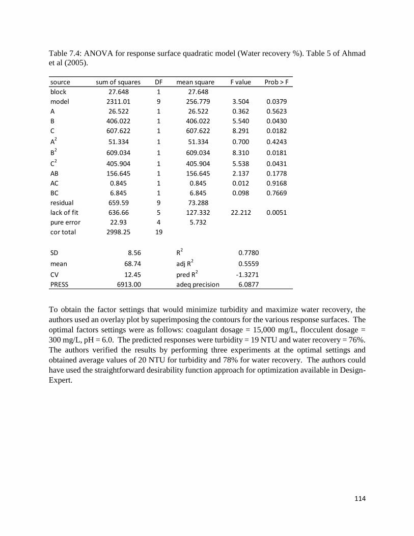
114
Table 7.4: ANOVA for response surface quadratic model (Water recovery %). Table 5 of Ahmad
et al (2005).
To obtain the factor settings that would minimize turbidity and maximize water recovery, the
authors used an overlay plot by superimposing the contours for the various response surfaces. The
optimal factors settings were as follows: coagulant dosage = 15,000 mg/L, flocculent dosage =
300 mg/L, pH = 6.0. The predicted responses were turbidity = 19 NTU and water recovery = 76%.
The authors verified the results by performing three experiments at the optimal settings and
obtained average values of 20 NTU for turbidity and 78% for water recovery. The authors could
have used the straightforward desirability function approach for optimization available in Design-
Expert.
source sum of squares DF mean square F value Prob > F
block 27.648 1 27.648
model 2311.01 9 256.779 3.504 0.0379
A 26.522 1 26.522 0.362 0.5623
B 406.022 1 406.022 5.540 0.0430
C 607.622 1 607.622 8.291 0.0182
A2
51.334 1 51.334 0.700 0.4243
B2 609.034 1 609.034 8.310 0.0181
C2 405.904 1 405.904 5.538 0.0431
AB 156.645 1 156.645 2.137 0.1778
AC 0.845 1 0.845 0.012 0.9168
BC 6.845 1 6.845 0.098 0.7669
residual 659.59 9 73.288
lack of fit 636.66 5 127.332 22.212 0.0051
pure error 22.93 4 5.732
cor total 2998.25 19
SD 8.56 R2 0.7780
mean 68.74 adj R2
0.5559
CV 12.45 pred R2
-1.3271
PRESS 6913.00 adeq precision 6.0877
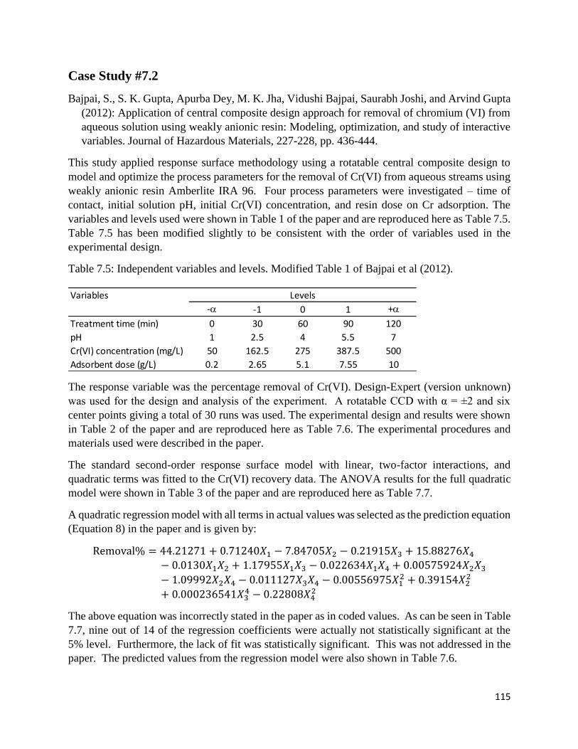
115
Case Study #7.2
Bajpai, S., S. K. Gupta, Apurba Dey, M. K. Jha, Vidushi Bajpai, Saurabh Joshi, and Arvind Gupta
(2012): Application of central composite design approach for removal of chromium (VI) from
aqueous solution using weakly anionic resin: Modeling, optimization, and study of interactive
variables. Journal of Hazardous Materials, 227-228, pp. 436-444.
This study applied response surface methodology using a rotatable central composite design to
model and optimize the process parameters for the removal of Cr(VI) from aqueous streams using
weakly anionic resin Amberlite IRA 96. Four process parameters were investigated – time of
contact, initial solution pH, initial Cr(VI) concentration, and resin dose on Cr adsorption. The
variables and levels used were shown in Table 1 of the paper and are reproduced here as Table 7.5.
Table 7.5 has been modified slightly to be consistent with the order of variables used in the
experimental design.
Table 7.5: Independent variables and levels. Modified Table 1 of Bajpai et al (2012).
The response variable was the percentage removal of Cr(VI). Design-Expert (version unknown)
was used for the design and analysis of the experiment. A rotatable CCD with α = ±2 and six
center points giving a total of 30 runs was used. The experimental design and results were shown
in Table 2 of the paper and are reproduced here as Table 7.6. The experimental procedures and
materials used were described in the paper.
The standard second-order response surface model with linear, two-factor interactions, and
quadratic terms was fitted to the Cr(VI) recovery data. The ANOVA results for the full quadratic
model were shown in Table 3 of the paper and are reproduced here as Table 7.7.
A quadratic regression model with all terms in actual values was selected as the prediction equation
(Equation 8) in the paper and is given by:
Removal% = 44.21271 + 0.71240𝑋1 − 7.84705𝑋2 − 0.21915𝑋3 + 15.88276𝑋4− 0.0130𝑋1𝑋2 + 1.17955𝑋1𝑋3 − 0.022634𝑋1𝑋4 + 0.00575924𝑋2𝑋3− 1.09992𝑋2𝑋4 − 0.011127𝑋3𝑋4 − 0.00556975𝑋1
2 + 0.39154𝑋22
+ 0.000236541𝑋34 − 0.22808𝑋4
2
The above equation was incorrectly stated in the paper as in coded values. As can be seen in Table
7.7, nine out of 14 of the regression coefficients were actually not statistically significant at the
5% level. Furthermore, the lack of fit was statistically significant. This was not addressed in the
paper. The predicted values from the regression model were also shown in Table 7.6.
Variables
- -1 0 1 +
Treatment time (min) 0 30 60 90 120
pH 1 2.5 4 5.5 7
Cr(VI) concentration (mg/L) 50 162.5 275 387.5 500
Adsorbent dose (g/L) 0.2 2.65 5.1 7.55 10
Levels
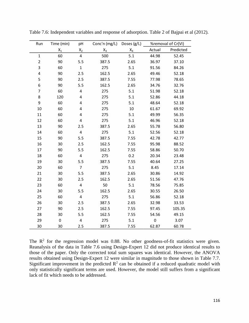
116
Table 7.6: Independent variables and response of adsorption. Table 2 of Bajpai et al (2012).
The R2 for the regression model was 0.88. No other goodness-of-fit statistics were given.
Reanalysis of the data in Table 7.6 using Design-Expert 12 did not produce identical results to
those of the paper. Only the corrected total sum squares was identical. However, the ANOVA
results obtained using Design-Expert 12 were similar in magnitude to those shown in Table 7.7.
Significant improvement in the predicted R2 can be obtained if a reduced quadratic model with
only statistically significant terms are used. However, the model still suffers from a significant
lack of fit which needs to be addressed.
Run Time (min) pH Conc'n (mg/L) Doses (g/L)
X1 X2 X3 X4 Actual Predicted
1 60 4 500 5.1 44.98 52.45
2 90 5.5 387.5 2.65 36.97 37.10
3 60 1 275 5.1 91.56 84.26
4 90 2.5 162.5 2.65 49.46 52.18
5 90 2.5 387.5 7.55 77.98 78.65
6 90 5.5 162.5 2.65 34.76 32.76
7 60 4 275 5.1 51.98 52.18
8 120 4 275 5.1 52.86 44.18
9 60 4 275 5.1 48.64 52.18
10 60 4 275 10 61.67 69.92
11 60 4 275 5.1 49.99 56.35
12 60 4 275 5.1 46.96 52.18
13 90 2.5 387.5 2.65 55.78 56.80
14 60 4 275 5.1 52.56 52.18
15 90 5.5 387.5 7.55 42.78 42.77
16 30 2.5 162.5 7.55 95.98 88.52
17 90 5.5 162.5 7.55 58.86 50.70
18 60 4 275 0.2 20.34 23.48
19 30 5.5 387.5 7.55 40.64 27.25
20 60 7 275 5.1 8.45 17.14
21 30 5.5 387.5 2.65 30.86 14.92
22 30 2.5 162.5 2.65 51.56 47.76
23 60 4 50 5.1 78.56 75.85
24 30 5.5 162.5 2.65 30.55 26.50
25 60 4 275 5.1 56.86 52.18
26 30 2.5 387.5 2.65 32.98 33.53
27 90 2.5 162.5 7.55 97.45 105.35
28 30 5.5 162.5 7.55 54.56 49.15
29 0 4 275 5.1 0 3.07
30 30 2.5 387.5 7.55 62.87 60.78
%removal of Cr(VI)

117
Table 7.7: ANOVA table for response surface quadratic model. Table 3 of Bajpai et al (2012).
The authors then used quadratic programming to determine the optimal conditions to maximize
Cr(VI) removal using the developed regression model. The optimal conditions obtained using
Amberlite IRA 96 resin in a batch process at temperature 30 °C were: contact time of 62.56 min,
initial solution pH of 1.96, initial Cr(VI) concentration of 145.4 mg/L, and adsorbent dose of 8.51
g/L. With these conditions, the model predicted a 94.90% removal of Cr(VI). To validate the
conditions obtained, an experiment with the optimal settings was conducted. The results were
shown in Table 4 of the paper and are reproduced here as Table 7.8.
Table 7.8: Model validation. Table 4 of Bajpai et al (2012).
More than one validation experiment would provide more confidence in the developed model. The
authors could have used the desirability function approach for optimization that is available in
Design-Expert instead of using quadratic programming.
Source Sum of squares df Mean square F value p value > F
Model 13,080.82 14 934.34 7.70 0.0002
X1 - time 862.69 1 862.69 7.11 0.0176
X2 - pH 4715.57 1 4715.57 38.88 0.0001
X3 - conc. 942.77 1 942.77 7.77 0.0138
X4 - dose 3197.51 1 3197.51 26.36 0.0001
X1X2 5.38 1 5.38 0.04 0.0836
X1X3 284.21 1 284.21 2.34 0.1467
X1X4 41.89 1 41.89 0.35 0.5655
X2X3 18.84 1 18.84 0.16 0.6991
X2X4 257.11 1 257.11 2.12 0.1660
X3X4 170.65 1 170.65 1.41 0.2540
X12
696.84 1 696.84 5.74 0.0300
X22 21.52 1 21.52 0.18 0.6796
X32 311.07 1 311.07 2.56 0.1301
X42
51.98 1 51.98 0.43 0.5226
Residual 1819.49 15 121.3
Lack of fit 1757.53 10 175.75 14.18 0.0046
Pure error 61.96 5 12.39
Cor total 14,900.32 29
pH Adsorbent Time Initial Cr(VI)
dose (g/L) (min) conc'n (mg/L) predicted actual
1.96 8.51 62.5 145.4 94.99 93.26
% removal

118
Case Study #7.3
Eren, I. and Figen Kaymak-Erktekin (2007): Optimization of osmotic dehydration of potato using
response surface methodology. Journal of Food Engineering, 79, pp. 344-352.
This study used response surface methodology with a rotatable central composite design to
determine the optimum conditions to dehydrate potatoes by osmotic dehydration to maximize
water loss and weight reduction, and minimize solid gain and water activity. Osmotic dehydration
is gaining in popularity in food processing due to its energy efficiency and quality produced. Four
factors were investigated – temperature, sucrose concentration, salt concentration, and processing
time. The factors and levels used in the experiment are summarized in Table 7.9.
Table 7.9: Factors and levels used in potato dehydration experiment.
The materials and methods used in the osmotic dehydration process were described in the paper.
The responses of interest were: water loss (WL, %), weight reduction (WR, %), solid gain (SG,
%) and water activity (aw). The definitions of the responses and how they were measured were
given in the paper. The goal was to determine the optimal settings of the four process parameters
(factors) to maximize WL and WR, while minimizing SG and aw.
Design-Expert 6.01 was used in the design and analyses of the experiment, and also in subsequent
optimization using the developed model.
A four-factor rotatable CCD with = ±2, and seven center points was used. The total number of
runs was 31 (16 factorial points, 8 axial points, and 7 center points). The experimental matrix and
results were shown in Table 1 of the paper and are reproduced here as Table 7.10.
A full standard second-order quadratic response surface model was then fitted to each of the
responses. The full ANOVA table and associated regression coefficients were summarized in
Table 2 of the paper and are reproduced here as Table 7.11 (typographical errors in the original
table have been corrected in Table 7.11).
The full quadratic model provided a reasonably good fit to each of the responses and the lack of
fit tests were all statistically insignificant at the 5% level. Reanalyses of the data in Table 7.10
gave similar results to those reported in Table 7.11 but not identical. Higher predicted R2 values
could be obtained by using reduced quadratic models with only statistically significant terms.
Variable Name Unit -2 -1 0 1 2
x1 Temperature °C 20 30 40 50 60
x2 Sucrose concentration % 40 45 50 55 60
x3 Salt concentration % 0 3.75 7.5 11.25 15
x4 Time min 29.5 142 254.5 367 479.5
Levels

119
Table 7.10: Central composite rotatable design with experimental values of response variables.
Table 1 of Eren et al (2007).
The authors then used the desirability function approach available in Design-Expert to determine
the optimum conditions for osmotic dehydration of potatoes. The goals were to maximize water
loss and weight reduction and minimize solid gain and water activity. The optimal conditions
were found to be: temperature of 22 °C, sucrose concentration of 54.5%, salt concentration of 14%,
and time of 329 min, obtaining a water loss of 59.1 (g/100g fresh sample), weight reduction of
52.9 (g/100g fresh sample), solid gain of 6.0 (g/100g fresh sample), and water activity of 0.785.
No further experiments were conducted to validate the optimum conditions obtained.
Run # Temp Sucrose Salt Time WL SG WR aw
(°C) conc. (%) Conc. (%) (min) (%) (%) (%)
1 30 (-1) 45 3.75 142 40 3.6 36.4 0.954
2 50 (+1) 45 3.75 142 46.9 4.5 42.5 0.931
3 30 (-1) 55 3.75 142 46.2 4 42.2 0.942
4 50 (+1) 55 3.75 142 54.6 5.5 49 0.919
5 30 (-1) 45 11.25 142 48.6 5 43.5 0.878
6 50 (+1) 45 11.25 142 56 6.6 49.4 0.855
7 30 (-1) 55 11.25 142 54.2 5.9 48.3 0.861
8 50 (+1) 55 11.25 142 60.5 7.1 53.4 0.828
9 30 (-1) 45 3.75 367 48.9 5.8 43.1 0.929
10 50 (+1) 45 3.75 367 52 7.4 44.6 0.919
11 30 (-1) 55 3.75 367 55.9 6.5 49.5 0.911
12 50 (+1) 55 3.75 367 60.5 8 52.5 0.896
13 30 (-1) 45 11.25 367 56.9 7 49.8 0.849
14 50 (+1) 45 11.25 367 58.6 8.2 50.4 0.838
15 30 (-1) 55 11.25 367 61.4 7.4 54 0.816
16 50 (+1) 55 11.25 367 64.8 8.6 56.2 0.798
17 20 (-2) 50 7.5 254.5 54.6 4.3 50.3 0.897
18 60 (+2) 50 7.5 254.5 62.2 7.6 54.6 0.864
19 40 (0) 40 7.5 254.5 50.3 7 43.3 0.891
20 40 (0) 60 7.5 254.5 62.8 8.1 54.7 0.846
21 40 (0) 50 0 254.5 43.4 5.1 38.3 0.957
22 40 (0) 50 15 254.5 61.9 6.7 55.1 0.778
23 40 (0) 50 7.5 29.5 40.9 3.7 37.2 0.941
24 40 (0) 50 7.5 479.5 60.6 9.3 51.3 0.871
25 40 (0) 50 7.5 254.5 60.5 7 53.4 0.878
26 40 (0) 50 7.5 254.5 60.5 6.5 53.9 0.869
27 40 (0) 50 7.5 254.5 61.5 7.1 54.4 0.874
28 40 (0) 50 7.5 254.5 60.6 6.8 53.7 0.876
29 40 (0) 50 7.5 254.5 61.9 6.4 55.5 0.878
30 40 (0) 50 7.5 254.5 59.1 6.4 52.8 0.88
31 40 (0) 50 7.5 254.5 63.7 6.8 56.9 0.881

120
Table 7.11: ANOVA table showing the variables as linear, quadratic and interaction terms on each
response variable and coefficients for the prediction models. Corrected Table 2 of Eren et al
(2007).
Case Study #7.4
Lakshminarayanan, A. K., V. E. Annamalai, and K. Elangovan (2015): Identification of optimum
friction stir spot welding process parameters controlling the properties of low carbon
automotive steel joints. Journal of Materials Research and Technology, 4 (3), pp. 262-272.
This study applied response surface methodology using a rotatable central composite design to
optimize the process parameters for friction stir spot welding of low carbon automotive steel joints.
The goal was to develop a model for predicting the lap shear tensile strength of the welded steel
joints and to determine the optimum settings of the process parameters to maximize strength. Three
process parameters – rotational speed, plunge depth, and dwell time were investigated. The
parameters and levels used in the experiment were shown in Table 3 of the paper and are
reproduced here as Table 7.12. The details of the experimental work and materials used were
described in the paper. The response of interest was the tensile shear failure load (TSFL) in kN.
Source DF
Coefficient Sum of p-value Coefficient Sum of p-value Coefficient Sum of p-value Coefficient Sum of p-value
squares squares squares squares
Intercept/Model 14 61.110 1431.26 <0.0001 6.729 59.90 <0.0001 54.380 1012.82 <0.0001 0.877 0.058 <0.0001
x1 1 2.373 135.14 <0.0001 0.723 12.54 <0.0001 1.650 65.34 <0.0001 -0.009 0.0021 <0.0001
x2 1 3.139 236.45 <0.0001 0.296 2.10 0.0008 2.843 193.95 <0.0001 -0.011 0.0031 <0.0001
x3 1 3.870 359.35 <0.0001 0.578 8.01 <0.0001 3.292 260.07 <0.0001 -0.043 0.045 <0.0001
x4 1 3.811 348.63 <0.0001 1.160 32.30 <0.0001 2.651 168.70 <0.0001 -0.015 0.0052 <0.0001
x12 1 -0.753 16.22 0.0205 -0.220 1.38 0.0041 -0.533 8.14 0.0792 0.001 5E-05 0.1108
x22 1 -1.211 41.97 0.0008 0.187 1.00 0.0117 -1.398 55.91 0.0001 -0.002 8E-05 0.0518
x32 1 -2.190 137.21 <0.0001 -0.227 1.47 0.0032 -1.964 110.26 <0.0001 -0.002 0.0001 0.0280
x42 1 -2.666 203.26 <0.0001 -0.078 0.17 0.2518 -2.588 191.54 <0.0001 0.008 0.0017 <0.0001
x1x2 1 0.215 0.74 0.5898 0.003 0.00 0.9765 0.213 0.72 0.5796 -0.001 3E-05 0.2123
x1x3 1 -0.245 0.96 0.5409 -0.032 0.02 0.7189 -0.212 0.72 0.5800 -0.001 1E-05 0.4206
x1x4 1 -1.005 16.16 0.0207 0.028 0.01 0.7505 -1.033 17.09 0.0143 0.003 0.0001 0.0120
x2x3 1 -0.520 4.39 0.1996 -0.034 0.02 0.7065 -0.490 3.84 0.2111 -0.003 0.0002 0.0073
x2x4 1 0.140 0.32 0.7241 -0.049 0.04 0.5812 0.190 0.58 0.6204 -0.003 0.0001 0.0153
x3x4 1 -0.440 3.07 0.2796 -0.202 0.65 0.0349 -0.236 0.89 0.5393 -0.002 7E-05 0.0955
Residual 16 39.23 1.97 36.24 0.0003
Lack of fit 10 26.75 0.3944 1.49 0.2295 24.69 0.3952 0.0002 0.4624
Pure error 6 12.48 0.48 11.54 0.0001
Total 30 1470.49 61.87 1049.06 0.058
R2 0.9733 0.9682 0.9655 0.995
Adj-R2 0.9500 0.9403 0.9352 0.9907
Pred-R2 0.8837 0.8507 0.8494 0.9791
PRESS 171.07 9.23 157.95 0.0012
CV 2.80 5.42 3.05 0.48
Water Loss (WL) Solid gain (SG) Weight reduction (WR) Water activity (aw)
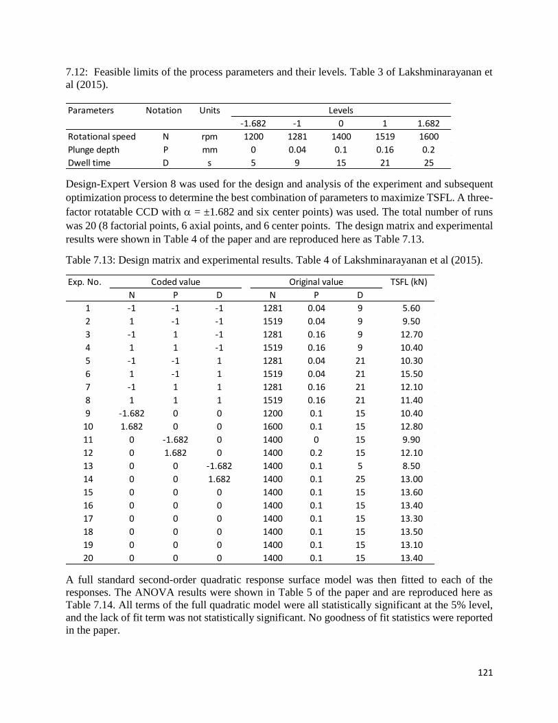
121
7.12: Feasible limits of the process parameters and their levels. Table 3 of Lakshminarayanan et
al (2015).
Design-Expert Version 8 was used for the design and analysis of the experiment and subsequent
optimization process to determine the best combination of parameters to maximize TSFL. A three-
factor rotatable CCD with = ±1.682 and six center points) was used. The total number of runs
was 20 (8 factorial points, 6 axial points, and 6 center points. The design matrix and experimental
results were shown in Table 4 of the paper and are reproduced here as Table 7.13.
Table 7.13: Design matrix and experimental results. Table 4 of Lakshminarayanan et al (2015).
A full standard second-order quadratic response surface model was then fitted to each of the
responses. The ANOVA results were shown in Table 5 of the paper and are reproduced here as
Table 7.14. All terms of the full quadratic model were all statistically significant at the 5% level,
and the lack of fit term was not statistically significant. No goodness of fit statistics were reported
in the paper.
Parameters Notation Units
-1.682 -1 0 1 1.682
Rotational speed N rpm 1200 1281 1400 1519 1600
Plunge depth P mm 0 0.04 0.1 0.16 0.2
Dwell time D s 5 9 15 21 25
Levels
Exp. No. TSFL (kN)
N P D N P D
1 -1 -1 -1 1281 0.04 9 5.60
2 1 -1 -1 1519 0.04 9 9.50
3 -1 1 -1 1281 0.16 9 12.70
4 1 1 -1 1519 0.16 9 10.40
5 -1 -1 1 1281 0.04 21 10.30
6 1 -1 1 1519 0.04 21 15.50
7 -1 1 1 1281 0.16 21 12.10
8 1 1 1 1519 0.16 21 11.40
9 -1.682 0 0 1200 0.1 15 10.40
10 1.682 0 0 1600 0.1 15 12.80
11 0 -1.682 0 1400 0 15 9.90
12 0 1.682 0 1400 0.2 15 12.10
13 0 0 -1.682 1400 0.1 5 8.50
14 0 0 1.682 1400 0.1 25 13.00
15 0 0 0 1400 0.1 15 13.60
16 0 0 0 1400 0.1 15 13.40
17 0 0 0 1400 0.1 15 13.30
18 0 0 0 1400 0.1 15 13.50
19 0 0 0 1400 0.1 15 13.10
20 0 0 0 1400 0.1 15 13.40
Coded value Original value
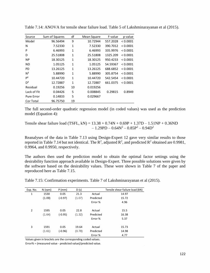
122
Table 7.14: ANOVA for tensile shear failure load. Table 5 of Lakshminarayanan et al (2015).
The full second-order quadratic regression model (in coded values) was used as the prediction
model (Equation 4):
Tensile shear failure load (TSFL, kN) = 13.38 + 0.74N + 0.69P + 1.37D – 1.51NP + 0.36ND
– 1.29PD – 0.64N2 – 0.85P2 – 0.94D2
Reanalyses of the data in Table 7.13 using Design-Expert 12 gave very similar results to those
reported in Table 7.14 but not identical. The R2, adjusted R2, and predicted R2 obtained are 0.9981,
0.9964, and 0.9950, respectively.
The authors then used the prediction model to obtain the optimal factor settings using the
desirability function approach available in Design-Expert. Three possible solutions were given by
the software based on the desirability values. These were shown in Table 7 of the paper and
reproduced here as Table 7.15.
Table 7.15: Confirmation experiments. Table 7 of Lakshminarayanan et al (2015).
Source Sum of Squares df Mean Square F-value p-value
Model 96.56494 9 10.72944 557.2028 < 0.0001
N 7.52330 1 7.52330 390.7012 < 0.0001
P 6.46993 1 6.46993 335.9976 < 0.0001
D 25.51808 1 25.51808 1325.209 < 0.0001
NP 18.30125 1 18.30125 950.4233 < 0.0001
ND 1.05125 1 1.05125 54.59367 < 0.0001
PD 13.26125 1 13.26125 688.6852 < 0.0001
N² 5.88990 1 5.88990 305.8754 < 0.0001
P² 10.44720 1 10.44720 542.5454 < 0.0001
D² 12.72887 1 12.72887 661.0375 < 0.0001
Residual 0.19256 10 0.019256
Lack of Fit 0.04426 5 0.008845 0.29815 0.8949
Pure Error 0.14833 5 0.029667
Cor Total 96.75750 19
Exp. No. N (rpm) P (mm) D (s) Tensile shear failure load (kN)
1 1530 0.05 21.3 Actual 14.97
(1.09) (-0.97) (1.07) Predicted 15.72
Error % 4.96
2 1595 0.05 22.8 Actual 15.5
(1.64) (-0.95) (1.32) Predicted 16.38
Error % 5.37
3 1591 0.05 19.64 Actual 15.73
(1.61) (-0.96) (0.78) Predicted 14.98
Error % 4.77
Values given in braclets are the corresponding coded values.
Error% = (measured value - predicted value)/predicted value.

123
Three confirmation experiments were conducted using the optimal combinations shown in the
table to validate the model. The predicted and observed values are also shown in Table 7.15. The
percentage errors were around 5%.
The authors concluded that a maximum tensile shear fracture load 15.67 kN could be attained
using a tool rotation speed of 1157 rpm, plunge depth of 0.05 mm, and dwell time of 22 s. It is not
clear how these values were obtained as they were not part of the optimal combinations shown in
Table 7.15.
Case Study #7.5
Mu, Y., Xian-Jun Zheng, and Han-Qing Yu (2009): Determining optimum conditions for hydrogen
production from glucose by an anaerobic culture using response surface methodology (RSM).
International Journal of Hydrogen Energy, 34, pp. 7959-7963.
This study applied response surface methodology using a rotatable central composite design to
optimize the production of H2 from glucose by an anaerobic culture. Three factors that influenced
the hydrogen production process – temperature, pH, and glucose concentration were investigated.
The factors and levels used are summarized in Table 7.16. The experimental methods and
materials used in the experiment were described in the paper.
Table 7.16: Factors and levels used in the hydrogen production experiment.
The response of interest was the H2 yield (mol-H2/mol-glucose). The primary goal was to
determine the optimal combinations of the three factors to maximize H2 yield.
A three-factor rotatable CCD with = ±1.68 and six center points was used. The total number of
runs was 20 (8 factorial points, 6 axial points, and 6 center points.) Minitab (unknown version)
was used for the design and analysis of the experiment. The design matrix in coded and real values,
and H2 yield results were shown in Table 1 of the paper and are reproduced here as Table 7.17.
A full standard second-order quadratic response surface model was fitted to the response and the
estimated regression coefficients and associated statistics were shown in Table 2 of the paper and
are reproduced here as Table 7.18. Six of the coefficients were not statistically significant at the
5% level. However, the authors seem to have used the full model in the optimization phase.
The summarized ANOVA table for the full model was shown in Table 3 of the paper and is
reproduced here as Table 7.19. The only goodness of fit statistic was the R2 value of 0.927. There
was no mention of regression diagnostics in the paper.
Factor Units
-1.68 -1 0 1 1.68
Temperature °C 27.4 32.5 40 47.5 52.6
pH 4.24 4.75 5.5 6.25 6.76
Glucose concentration g/L 5.8 7.5 10 12.5 14.2
Levels
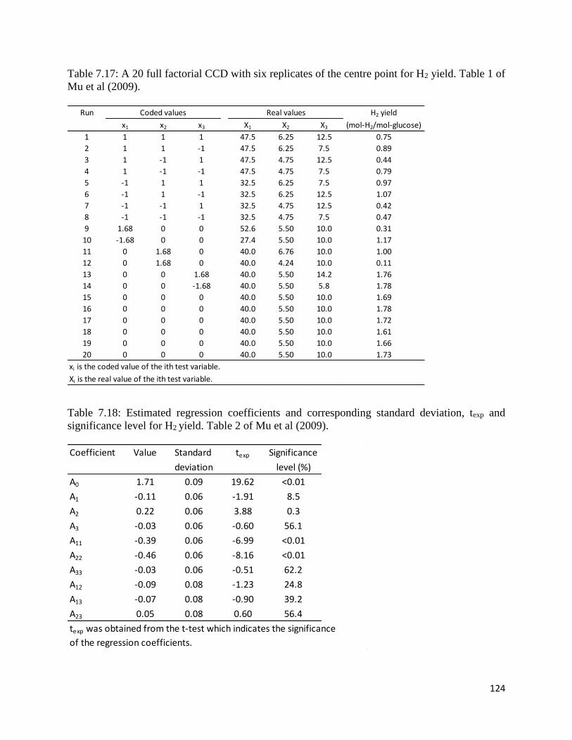
124
Table 7.17: A 20 full factorial CCD with six replicates of the centre point for H2 yield. Table 1 of
Mu et al (2009).
Table 7.18: Estimated regression coefficients and corresponding standard deviation, texp and
significance level for H2 yield. Table 2 of Mu et al (2009).
Run H2 yield
x1 x2 x3 X1 X2 X3 (mol-H2/mol-glucose)
1 1 1 1 47.5 6.25 12.5 0.75
2 1 1 -1 47.5 6.25 7.5 0.89
3 1 -1 1 47.5 4.75 12.5 0.44
4 1 -1 -1 47.5 4.75 7.5 0.79
5 -1 1 1 32.5 6.25 7.5 0.97
6 -1 1 -1 32.5 6.25 12.5 1.07
7 -1 -1 1 32.5 4.75 12.5 0.42
8 -1 -1 -1 32.5 4.75 7.5 0.47
9 1.68 0 0 52.6 5.50 10.0 0.31
10 -1.68 0 0 27.4 5.50 10.0 1.17
11 0 1.68 0 40.0 6.76 10.0 1.00
12 0 1.68 0 40.0 4.24 10.0 0.11
13 0 0 1.68 40.0 5.50 14.2 1.76
14 0 0 -1.68 40.0 5.50 5.8 1.78
15 0 0 0 40.0 5.50 10.0 1.69
16 0 0 0 40.0 5.50 10.0 1.78
17 0 0 0 40.0 5.50 10.0 1.72
18 0 0 0 40.0 5.50 10.0 1.61
19 0 0 0 40.0 5.50 10.0 1.66
20 0 0 0 40.0 5.50 10.0 1.73
xi is the coded value of the ith test variable.
Xi is the real value of the ith test variable.
Coded values Real values
Coefficient Value Standard texp Significance
deviation level (%)
A0 1.71 0.09 19.62 <0.01
A1 -0.11 0.06 -1.91 8.5
A2 0.22 0.06 3.88 0.3
A3 -0.03 0.06 -0.60 56.1
A11 -0.39 0.06 -6.99 <0.01
A22 -0.46 0.06 -8.16 <0.01
A33 -0.03 0.06 -0.51 62.2
A12 -0.09 0.08 -1.23 24.8
A13 -0.07 0.08 -0.90 39.2
A23 0.05 0.08 0.60 56.4
texp was obtained from the t-test which indicates the significance
of the regression coefficients.

125
Table 7.19: ANOVA analysis. Table 3 of Mu et al (2009).
Reanalysis of the data in Table 7.17 using Design-Expert 12 gave almost identical results to those
reported in the paper. However, the lack of fit was statistically significant (p-value = 0.0015), and
Run #10 was identified as an outlier. The predicted R2 was also quite low (0.4667). Furthermore
if a reduced model with only statistically significant terms was used, the predicted R2 would have
increased by over 20%.
It is not clear exactly how the authors obtained the optimum conditions of a temperature of 38.8
°C, pH of 5.7, and glucose concentration of 9.7 g/L giving a maximum H2 yield of 1.75 mol-
H2/mol-glucose. No additional experiments were conducted to confirm the model and optimum
conditions obtained.
Case Study #7.6
Prasad, K. N., Fouad Abdulrahman Hassan, Bao Yang, Kin Weng Kong, Ramakrishnan
Nagasundara Ramanan, Azrina Azlan, and Amin Ismail (2011): Response surface optimization
for the extraction of phenolic compounds and antioxidant capacities of underutilised Mangifera
pajang Kosterm peels. Food Chemistry, 1238, pp. 1121-1127.
This study used response surface methodology with a rotatable central composite design to
optimize the conditions for the maximum recovery of total phenolics content (TPC) and
antioxidant capacities (AC) of Mangifera pajang peels (MPP). Mangifera pajang is an
underutilized fruit from East Malaysia, and is commonly referred to as brown mango or
bambangan in the Malay language. Three factors – ethanol concentration, extraction temperature,
and liquid-to-solid ratio were investigated. The factors and levels used were shown in Table 1 of
the paper and are reproduced here as Table 7.20.
The primary objective of the study was to maximize the extraction of total phenolic content (TPC)
and the antioxidant capacity (AC) from the Mangifera pajang peels (MPP). The materials and
methods used were described in the paper.
Source Degree of Sum of Mean F- P-
freedom square square value value
Regression 9 5.8025 0.6447 14.18 0
Residual 10 0.4547 0.0455
Total 19 6.2573
R2 = 0.927
The Fisher variance ratio (F-value) is the ratio of the mean square
due to regression, divided by the mean square due to residual.

126
Table 7.20: Independent variables and their coded and actual values used for optimization. Table
1 of Prasad et al (2011).
Design-Expert 6.0 software was used for the experimental design and statistical analysis of the
responses. A three-factor rotatable CCD with = ±1.68 and six center points was used. The total
number of experimental runs was 20 consisting of eight factorial, six axial, and six center points.
The experimental design and results were shown in Table 2A of the paper and are reproduced here
as Table 7.21.
Table 7.21: Three-factor central composite design used for RSM with experimental and predicted
values for the independent variables. Table 2A of Prasad et al (2011).
Note that in Table 7.21, the first column heading should have been “Run #” as the order of runs
shown was not quite in standard order.
A full standard second-order quadratic response surface model was fitted to the responses but no
ANOVA results were shown in the paper. However, the estimated regression coefficients of the
polynomial models and some associated statistics were shown in Table 2B of the paper and are
reproduced here as Table 7.22. The predicted values of the two responses using the equations
shown in Table 7.22 were also shown in Table 7.21.
Independent variable Units Symbol
-1 0 1 Axial (-) Axial (+)
Ethanol concentration % X1 32 50 68 20 80
Temperature °C X2 37 48 58 30 65
Liquid/solid ratio mL/g X3 201 31.3 42.4 12.5 50
Coded levels
Standard order Factor 1 (X1) Factor 2 (X2) Factor 3 (X3)
Ethanol concentration (%) Temperature (°C) Liquid/soild ratio (mL/g)
Experimental Predicted Experimental Predicted
1 -1 -1 -1 6.39 6.04 0.165 0.166
2 1 -1 -1 7.19 7.36 0.186 0.188
3 -1 1 -1 6.41 6.51 0.135 0.135
4 1 1 -1 12.30 b 0.195 b
5 -1 -1 1 8.49 8.56 0.187 0.187
6 1 -1 1 10.20 9.88 0.183 0.183
7 -1 1 1 10.70 10.6 0.167 0.166
8 1 1 1 14.20 14.4 0.201 0.2
9a 0 0 0 13.70 13.5 0.203 0.203
10a 0 0 0 13.20 13.5 0.201 0.203
11a 0 0 0 13.40 13.5 0.206 0.203
12a 0 0 0 13.50 13.5 0.201 0.203
13 -1.68 0 0 5.97 6.11 0.142 0.143
14 1.68 0 0 10.40 10.4 0.191 0.19
15 0 -1.68 0 6.84 7.05 0.197 0.195
16 0 1.68 0 11.30 11.2 0.181 0.183
17 0 0 -1.68 6.01 6.02 0.166 0.165
18 0 0 1.68 11.50 11.6 0.185 0.187
19a 0 0 0 12.90 12.8 0.204 0.202
20a 0 0 0 13.00 12.8 0.201 0.202
a - Centre point
b - Outlier.
Response 1 (Y1)
TPC (mg GAE/g)
Response 2 (Y2)
AC (absorbance in nm)

127
In Table 7.21, run #4 was identified as an outlier and no predicted values were given. Upon a closer
examination of the predicted values, all center point values should have been identical, but this
was not the case in Table 7.21.
Reanalysis of the data in Table 7.21 using Design-Expert 12 gave almost identical results to those
reported for the second response AC (Y2) except that the lack of fit “p-value” was 0.3266 instead
of the reported 0.4764. All regression terms were statistically significant at the 5% level. However,
for the response TPC (Y1), the regression coefficients reported seemed to be off by several orders
of magnitude and the lack of fit was statistically significant at the 5% level (p-value = 0.011) and
not 0.1870 as reported. Furthermore, the interaction term X2X3 was also not statistically significant
at the 5% level and should not have beeen in the model. Run #4 would not be an outlier if a
reduced quadratic model with only statistically significant terms were used. Hence, the results
reported in Table 7.22 were mostly incorrect likely because of typographical errors, especially for
the magnitudes of the regression coefficients for TPC.
Table 7.22: Polynomial equation and statistical parameters calculated after implementation of 2nd
full factorial central composite experimental design. Corrected Table 2B of Prasad et al (2011).
Column 1 of Table 2B was incorrectly labelled as “Regression coefficient”.
The authors used a combination of graphical and numerical optimization methods to determine the
optimal levels of the independent variables to maximize TPC and AC. For the response TPC, the
optimum values were ethanol concentration of 68%, temperature of 55 °C, and liquid/solid ratio
of 32.7 mL/g. For the response AC, the optimum values were ethanol concentration of 68%,
temperature of 56 °C, and liquid/solid ratio of 31.8 mL/g. The predicted responses with these
settings were 14.6 mg GAE/g and 0.2065, respectively.
The response surface models were verified by conducting additional experiments at the optimum
values of the independent variables and the TPC and AC obtained experimentally were 14.6 ±
0.0026 mg GAE/g and 0.2035 ± 0, respectively.
No reasons were given as to why the optimization was not set to maximize both TPC and AC
simultaneously instead of individually, as was done in this study.
Response 2nd order polynomial equation R2 R2 (adjusted) Regression (p value) Lack of fit
TPC (Y1) 13158.69 + 1263.38X1 + 1235.93X2 + 1657.63X3 - 0.9969 0.9936 0.0001 0.1870
1615.12X12 - 1298.73X2
2 - 1409.43X32 + 605.41X1X2 + 397.40X2X3
AC (Y2) 0.20 + 0.014X1 - 0.00369X2 + 0.00651X3 - 0.012X12 - 0.9953 0.9900 0.0001 0.4764
0.00441X22 - 0.00922X3
2 - 0.00937X1X2 - 0.00626X1X3 + 0.00251X2X3

128
Case Study #7.7
Rastegar, S. O., S. M. Mousavi, S. A. Shojaosadati, and S. Sheibani (2011): Optimization of
petroleum refinery effluent treatment in a UASB reactor using response surface methodology.
Journal of Hazardous Materials, 197, pp. 26-32.
This study applied response surface methodology using a rotatable central composite design to
optimize the treatment of petroleum effluent in a laboratory scale upflow anaerobic sludge blanket
(UASB) bioreactor. The UASB bioreactor is a popular wastewater treatment used around the world
for several decades. The primary goal of this study was to investigate the phenomenon of removal
of petroleum refinery effluent in an UASB bioreactor. The schematic diagram of the UASB
bioreactor was given in the paper and the independent variables that were adjustable on the
bioreactor were the hydraulic retention time (HRT), upflow velocity (Vup), and the influent
chemical oxygen demand (COD). The experimental ranges and levels of the three variables were
shown in Table 2 of the paper and are reproduced here with corrections as Table 7.23.
Table 7.23: Experimental range and levels of independent test variables. Corrected Table 2 of
Rastegar et al (2011).
In Table 7.23, the variables are labelled to match the layout of the experimental design shown in
Table 3 of the paper. Hence, HRT is relabelled as A instead of B, influent COD is relabelled as C
instead of A, and Vup is relabelled as B instead of C.
Two responses were of interest – COD removal (%) and the biogas production rate (L biogas/L
feed d). Design-Expert 7.0 software was used for experimental design and statistical analysis. A
three-factor rotatable CCD with = ±1.68 and six center points was used. The total number of
experimental runs was 20 consisting of eight factorial, six axial, and six center points. The
experimental design and results were shown in Table 3 of the paper and are reproduced here as
Table 7.24.
A reduced quadratic response surface model was fitted to the COD removal data and a reduced
cubic model was fitted to the biogas rate data. The partial ANOVA results for the two responses
were shown in Table 4 of the paper and are reproduced here as Table 7.25. Only the R2 and adjusted
R2 values were shown.
For COD removal (%), the regression model was given as (Equation 2 in the paper):
COD removal (%) = 68.06 + 6.5A + 3.29B – 2.65C – 0.63AB + 0.87AC – 0.16A2
Note that from Table 7.25, the terms AB, AC, and A2 were not statistically significant at the 5%
level. Hence a linear model with only A, B, and C would be more correct.
Variable Low axial (-) Low factorial (-1) Center point (0) High factorial (+1) High axial (+)
HRT (h): A 10 12 17.5 22 25
Vup (m/h): B 0.1 0.18 0.3 0.42 0.5
Influent COD (mg/L): C 500 642 850 1060 1200

129
Table 7.24: Experimental plan and results. Table 3 of Rastegar et al (2011).
For biogas production rate, the regression model was given as (Equation 3 in the paper):
Biogas production rate (L biogas/L feed d) = 0.14 + 0.08A + 0.10B + 0.14C – 0.027AC - 0.02BC
+ 0.062A2+ 0.065C2 + 0.035B2 – 0.10A2B – 0.1AB2
Note that from Table 7.25, the terms AC and BC were not statistically significant at the 5% level.
Also, AB should be included for hierarchy.
Reanalyses of the data using Design-Expert 12 showed that both suggested models had statistically
significant lack of fit which was not reported. Furthermore, for COD removal, if only linear terms
were used, the predicted R2 would increase from 0.858 to 0.918.
For biogas production, the reported model actually had a predicted R2 of -0.0198. A negative
predicted R2 indicates that the model is no better than using the overall mean value. In addition,
some assumptions of regression were violated. The residuals were not normally distributed and
they were not homoscedastic. A logarithmic transformation of the response would provide a much
better fit and would not violate any regression assumptions. However, the lack of fit would still be
statistically significant.
Run HRT (h) Vup (m/h) Influent COD (mg/L) COD removal (%) Biogas rate (L biogas/L feed d)
1 22 0.42 642 78 0.18
2 22 0.18 642 72 0.14
3 17.5 0.3 851 68 0.15
4 17.5 0.1 851 61 0.1
5 17.5 0.5 851 74 0.44
6 13 0.42 642 68 0.17
7 10.0 0.3 851 55 0.21
8 22 0.42 1060 73 0.38
9 25 0.3 851 81 0.48
10 17.5 0.3 851 67 0.14
11 13 0.18 1060 54 0.52
12 17.5 0.3 851 69 0.14
13 17.5 0.3 851 68 0.14
14 17.5 0.3 1200 64 0.64
15 17.5 0.3 851 69 0.13
16 22 0.18 1060 70 0.33
17 13 0.18 642 63 0.13
18 17.5 0.3 500 73 0.07
19 17.5 0.3 851 69 0.13
20 13 0.42 1060 63 0.39

130
Table 7.25: ANOVA for response surface models applied. Table 4 of Rastegar et al (2011).
In the process optimization phase, the authors used graphical optimization to obtain the optimal
variable settings for a COD removal of 75% and biogas production rate of 0.20 L biogas/L feed d.
Reasons were given in the paper as to why these values for the responses were chosen. Two
experimental combinations were used to validate the models. The results of the validation
experiments were shown in Table 5 of the paper and are reproduced here as Table 7.26.
Table 7.26: Optimum condition verification and additional experiments. Table 5 of Rastegar et al
(2011).
The authors could have used the desirability function approach available in Design-Expert to
obtain the optimal combinations. Many other possible solutions are available to achieve the same
objective.
Response Model
Source Sum of square DF Mean square F value Prob > F
COD removal (%) Reduced quadratic Model 829.05 6 138.18 60.08 < 0.0001
model A 576.44 1 576.44 250.66 < 0.0001
B 147.38 1 147.38 64.09 < 0.0001
C 95.62 1 95.62 41.58 < 0.0001
A² 0.3659 1 0.37 0.1591 0.6965
AC 6.13 1 6.13 2.66 0.1267
AB 3.13 1 3.13 1.36 0.2647
Residual 29.90 13 2.30
(R2=0.96, R
2 adj = 0.94)
Biogas production rate Reduced cubic Model 0.502 10 0.050 18.48 < 0.0001
(L biogas/L feed d) model A-HRT (h) 0.036 1 0.036 13.42 0.0052
B-Vup (m/h) 0.058 1 0.058 21.29 0.0013
C-Influent COD 0.281 1 0.28 103.44 < 0.0001
AC 0.006 1 0.006 2.23 0.1697
BC 0.003 1 0.003 1.18 0.3000
A² 0.055 1 0.055 20.11 0.0015
C² 0.061 1 0.061 22.48 0.0011
B² 0.018 1 0.018 6.52 0.0311
A²B 0.034 1 0.034 12.47 0.0064
AB² 0.035 1 0.035 12.89 0.0058
Residual 0.024 9 0.0025
(R2=0.95, R2 adj = 0.90)
ANOVA
Influent COD HRT (h) Vup (m/h) COD removal (%) COD removal (%) Biogas rate (L/L feed d) Biogas rate (L/L feed d)
(mg/L) (model) (experiment) (model) (experiment)
630 21.4 0.27 75.0 76.3 0.2 0.25
620 21.4 0.27 74.9 78.3 0.2 0.24
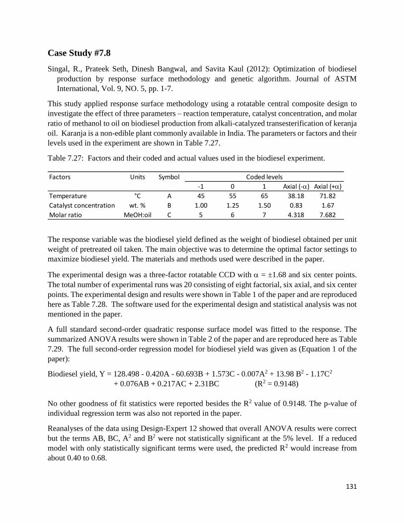
131
Case Study #7.8
Singal, R., Prateek Seth, Dinesh Bangwal, and Savita Kaul (2012): Optimization of biodiesel
production by response surface methodology and genetic algorithm. Journal of ASTM
International, Vol. 9, NO. 5, pp. 1-7.
This study applied response surface methodology using a rotatable central composite design to
investigate the effect of three parameters – reaction temperature, catalyst concentration, and molar
ratio of methanol to oil on biodiesel production from alkali-catalyzed transesterification of keranja
oil. Karanja is a non-edible plant commonly available in India. The parameters or factors and their
levels used in the experiment are shown in Table 7.27.
Table 7.27: Factors and their coded and actual values used in the biodiesel experiment.
The response variable was the biodiesel yield defined as the weight of biodiesel obtained per unit
weight of pretreated oil taken. The main objective was to determine the optimal factor settings to
maximize biodiesel yield. The materials and methods used were described in the paper.
The experimental design was a three-factor rotatable CCD with = ±1.68 and six center points.
The total number of experimental runs was 20 consisting of eight factorial, six axial, and six center
points. The experimental design and results were shown in Table 1 of the paper and are reproduced
here as Table 7.28. The software used for the experimental design and statistical analysis was not
mentioned in the paper.
A full standard second-order quadratic response surface model was fitted to the response. The
summarized ANOVA results were shown in Table 2 of the paper and are reproduced here as Table
7.29. The full second-order regression model for biodiesel yield was given as (Equation 1 of the
paper):
Biodiesel yield, Y = 128.498 - 0.420A - 60.693B + 1.573C - 0.007A2 + 13.98 B2 - 1.17C2
+ 0.076AB + 0.217AC + 2.31BC (R2 = 0.9148)
No other goodness of fit statistics were reported besides the R2 value of 0.9148. The p-value of
individual regression term was also not reported in the paper.
Reanalyses of the data using Design-Expert 12 showed that overall ANOVA results were correct
but the terms AB, BC, A2 and B2 were not statistically significant at the 5% level. If a reduced
model with only statistically significant terms were used, the predicted R2 would increase from
about 0.40 to 0.68.
Factors Units Symbol
-1 0 1 Axial (-) Axial (+)
Temperature °C A 45 55 65 38.18 71.82
Catalyst concentration wt. % B 1.00 1.25 1.50 0.83 1.67
Molar ratio MeOH:oil C 5 6 7 4.318 7.682
Coded levels

132
Table 7.28: Central composite design matrix. Table 1 of Singhal et al (2012).
Table 7.29: ANOVA results for the regression model. Table 2 of Singhal et al (2012).
Although not mentioned explicitly in the paper, optimization of biodiesel yield was likely obtained
using the desirability function approach with the constraints shown in Table 3 of the paper and
reproduced here as Table 7.30.
Table 7.30: Constraints used to optimize biodiesel yield. Table 3 of Singhal et al (2012).
The maximum biodiesel yield obtained was 97.86% at a temperature of 64.60 °C, catalyst
concentration of 1.0 wt %, and a molar ratio of methanol to oil of 6.996:1. Optimization using the
genetic algorithm approach apparently gave similar results.
Exp. No. Temperature (A) Catalyst conc. (B) Molar ratio (C) Yield (Y)
1 45 1 5 91.06
2 65 1 5 92.23
3 45 1.5 5 87.3
4 65 1.5 5 85.3
5 45 1 7 91.48
6 65 1 7 97.4
7 45 1.5 7 86.1
8 65 1.5 7 96.71
9 38.18 1.25 6 85.16
10 71.82 1.25 6 91.5
11 55 0.83 6 95.62
12 55 1.67 6 90
13 55 1.25 4.318 82.18
14 55 1.25 7.682 91.9
15 55 1.25 6 92
16 55 1.25 6 92.69
17 55 1.25 6 91.5
18 55 1.25 6 90.93
19 55 1.25 6 90.38
20 55 1.25 6 90.56
Source Degree of freedom (df) Sum of squares (SS) Mean sum of squares (MS) F p
Regression 9 258.2514 28.6946 11.9357 0.0003
Residual 10 24.0410 2.4041
Total 19 282.2924
Process variable Goal Lower limit Upper limit
A: Reaction temperature (°C) In range 45 65
B: Catalyst concentration (wt. %) In range 1.0 1.5
C: Molar ratio (MeOH:oil) In range 5 7
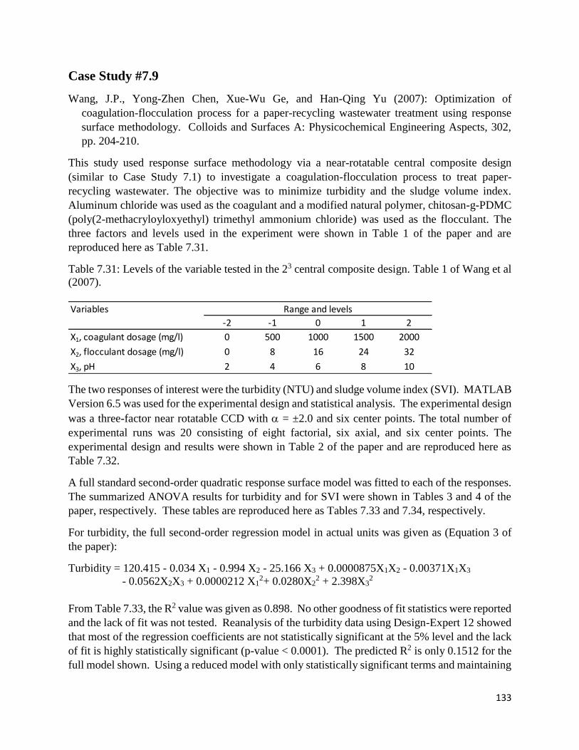
133
Case Study #7.9
Wang, J.P., Yong-Zhen Chen, Xue-Wu Ge, and Han-Qing Yu (2007): Optimization of
coagulation-flocculation process for a paper-recycling wastewater treatment using response
surface methodology. Colloids and Surfaces A: Physicochemical Engineering Aspects, 302,
pp. 204-210.
This study used response surface methodology via a near-rotatable central composite design
(similar to Case Study 7.1) to investigate a coagulation-flocculation process to treat paper-
recycling wastewater. The objective was to minimize turbidity and the sludge volume index.
Aluminum chloride was used as the coagulant and a modified natural polymer, chitosan-g-PDMC
(poly(2-methacryloyloxyethyl) trimethyl ammonium chloride) was used as the flocculant. The
three factors and levels used in the experiment were shown in Table 1 of the paper and are
reproduced here as Table 7.31.
Table 7.31: Levels of the variable tested in the 23 central composite design. Table 1 of Wang et al
(2007).
The two responses of interest were the turbidity (NTU) and sludge volume index (SVI). MATLAB
Version 6.5 was used for the experimental design and statistical analysis. The experimental design
was a three-factor near rotatable CCD with = ±2.0 and six center points. The total number of
experimental runs was 20 consisting of eight factorial, six axial, and six center points. The
experimental design and results were shown in Table 2 of the paper and are reproduced here as
Table 7.32.
A full standard second-order quadratic response surface model was fitted to each of the responses.
The summarized ANOVA results for turbidity and for SVI were shown in Tables 3 and 4 of the
paper, respectively. These tables are reproduced here as Tables 7.33 and 7.34, respectively.
For turbidity, the full second-order regression model in actual units was given as (Equation 3 of
the paper):
Turbidity = 120.415 - 0.034 X1 - 0.994 X2 - 25.166 X3 + 0.0000875X1X2 - 0.00371X1X3
- 0.0562X2X3 + 0.0000212 X12+ 0.0280X2
2 + 2.398X32
From Table 7.33, the R2 value was given as 0.898. No other goodness of fit statistics were reported
and the lack of fit was not tested. Reanalysis of the turbidity data using Design-Expert 12 showed
that most of the regression coefficients are not statistically significant at the 5% level and the lack
of fit is highly statistically significant (p-value < 0.0001). The predicted R2 is only 0.1512 for the
full model shown. Using a reduced model with only statistically significant terms and maintaining
Variables
-2 -1 0 1 2
X1, coagulant dosage (mg/l) 0 500 1000 1500 2000
X2, flocculant dosage (mg/l) 0 8 16 24 32
X3, pH 2 4 6 8 10
Range and levels
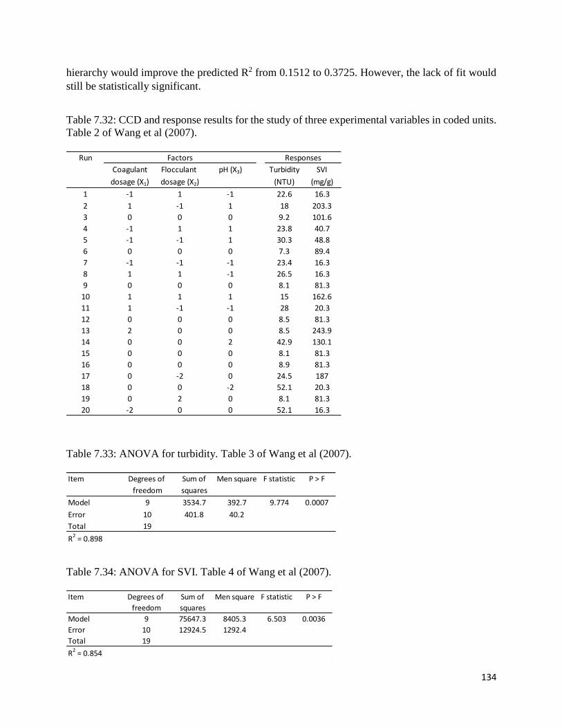
134
hierarchy would improve the predicted R2 from 0.1512 to 0.3725. However, the lack of fit would
still be statistically significant.
Table 7.32: CCD and response results for the study of three experimental variables in coded units.
Table 2 of Wang et al (2007).
Table 7.33: ANOVA for turbidity. Table 3 of Wang et al (2007).
Table 7.34: ANOVA for SVI. Table 4 of Wang et al (2007).
Run
Coagulant Flocculant pH (X3) Turbidity SVI
dosage (X1) dosage (X2) (NTU) (mg/g)
1 -1 1 -1 22.6 16.3
2 1 -1 1 18 203.3
3 0 0 0 9.2 101.6
4 -1 1 1 23.8 40.7
5 -1 -1 1 30.3 48.8
6 0 0 0 7.3 89.4
7 -1 -1 -1 23.4 16.3
8 1 1 -1 26.5 16.3
9 0 0 0 8.1 81.3
10 1 1 1 15 162.6
11 1 -1 -1 28 20.3
12 0 0 0 8.5 81.3
13 2 0 0 8.5 243.9
14 0 0 2 42.9 130.1
15 0 0 0 8.1 81.3
16 0 0 0 8.9 81.3
17 0 -2 0 24.5 187
18 0 0 -2 52.1 20.3
19 0 2 0 8.1 81.3
20 -2 0 0 52.1 16.3
ResponsesFactors
Item Degrees of Sum of Men square F statistic P > F
freedom squares
Model 9 3534.7 392.7 9.774 0.0007
Error 10 401.8 40.2
Total 19
R2 = 0.898
Item Degrees of Sum of Men square F statistic P > F
freedom squares
Model 9 75647.3 8405.3 6.503 0.0036
Error 10 12924.5 1292.4
Total 19
R2 = 0.854

135
For SVI, the full second-order regression model in actual units was given as (Equation 4 of the
paper):
SVI = 63.264 - 0.153X1 - 2.981X2 + 9.732X3 - 0.0011X1X2 + 0.034X1X3
- 0.350X2X3 + 0.0000292X12 + 0.130X2
2 - 1.604X32
The R2 value was 0.854. Similar to turbidity, no other goodness of fit statistics were reported.
Reanalysis of the SVI data using Design-Expert 12 showed that only factor X1, X3, and interaction
of X1 and X3 are statistically significant at the 5% level. Furthermore, the predicted R2 for the full
model is negative (-0.1527) indicating that the model is no better than the overall mean. The lack
of fit is also statistically significant (p-value = 0.0006). If a reduced model with only statistically
significant terms were used, the predicted R2 would improve to 0.592.
The authors then used each regression equation to perform optimization. For minimum turbidity,
the optimal conditions of the factors were coagulant dosage of 877 mg/l, flocculant dosage of 22.6
mg/l, and pH of 6.2, giving a turbidity value of 8.6 NTU.
For minimum SVI, the optimal conditions of the factors were coagulant dosage of 338 mg/l,
flocculant dosage of 19.1 mg/l, and pH of 4.5 giving a SVI of 30.9 ml/g. These results were verified
from additional experimental runs shown in Table 5 of the paper and are reproduced here as Table
7.35.
Table 7.35: Measured and calculated values for the confirmation experiments. Table 5 of Wang et
al (2007).
The authors then used multiple response optimization based on the desirability function approach
to determine the factor values to minimize both turbidity and SVI simultaneously. The optimal
factor values were a coagulant dosage of 759 mg/l, flocculant dosage of 22.3 mg/l, and pH of 5.4.
The corresponding turbidity and SVI obtained were 12.3 NTU and 48.0 ml/g, respectively.
Given the incorrect choice of models and the significant lack of fit of the chosen models, it is not
clear whether the results obtained are indeed accurate.
Run Conditions Parameter Measured Calculated
21 Coagulant dosage = 877 mg/l Turbidity (NTU) 8.7 ± 0.3 8.6
Flocculant dosage = 22.6 mg/l
pH = 6.2
22 Coagulant dosage = 338 mg/l SVI (ml/g) 32.5 ± 2.4 30.9
Flocculant dosage = 19.1 mg/l
pH = 4.5

136
Case Study #7.10
Yuan, X., Jia Liu, Guangming Zeng, Jingang Shi, Jingyi Tong, and Guohe Huang (2008):
Optimization of conversion of waste rapeseed oil with high FFA to biodiesel using response
surface methodology. Renewable Energy, 33, pp. 1678-1684.
This study used response surface methodology based on a 24 full-factorial rotatable central
composite design to investigate the conversion to biodiesel of waste rapeseed oil with high free
fatty acids as raw material to biodiesel. The goal was to maximize the conversion and to gain
insights into the process affecting biodiesel production. The four factors and levels investigated
were shown in Table 1 of the paper and are reproduced here as Table 7.36.
Table 7.36: Experimental range and levels of the independent variables. Table 1 of Yuan et al
(2008).
The materials and methods used in the experiment were described in the paper. Design-Expert 6.0
was used for the experimental design and statistical analysis of the data obtained. The response
variable was the conversion to biodiesel (wt. %). A rotatable CCD with α = ±2 and six center
points giving a total of 30 runs was used. The experimental design and results were shown in Table
2 of the paper and are reproduced here as Table 7.37.
The standard second-order response surface model with linear, two-factor interactions, and
quadratic terms was fitted to the response. The summarized ANOVA results together with the
goodness of fit statistics for the full quadratic model were shown in Table 3 of the paper and are
reproduced here as Table 7.38.
The estimated regression coefficients and associated statistics for the full model were shown in
Table 4 of the paper and are reproduced here as Table 7.39. The second-order regression equation
for biodiesel conversion was given as (Equation 2 of the paper):
Y = 83.03 + 0.80X1 + 0.67X2 - 0.17X3 + 0.58X4 - 0.68X12 - 5.05X2
2 -1.322X32 - 0.62X4
2
-0.30X1X2 + 0.65X1X3 - 0.39X1X4 - 1.18X2X3 + 6.875 x 10-3X2X4 + 0.027X3X4
Note that while the full model was highly statistically significant, several of the regression
coefficients (X1X2, X1X3, X1X4, X2X4, and X3X4), were not statistically significant at the 5% level.
Furthermore, there was statistically significant lack of fit (p-value=0.0411) of the full model.
Variables Symbol coded
-2 -1 0 1 2
Methanol/oil molar ratio X1 4:1 5:1 6:1 7:1 8:1
Catalyst concentration (%) X2 0.4 0.8 1.0 1.2 1.6
Reaction time (min) X3 45 55 65 75 85
Temperature (°C) X4 25 35 45 55 65
Range and levels

137
Table 7.37: Full factorial central composite design matrix of four variables in coded and natural
units along with the observed responses. Table 2 of Yuan et al (2008).
Table 7.38: Analysis of variance (ANOVA) for the quadratic model. Table 3 of Yuan et al
(2008).
CV = 1.75%, R2 = 0.9664, R = 0.9830, Adj. R2 = 0.9351.
No. X1 X2 X3 X4 Methanol/oil Catalyst Reaction time T (°C) Conversion to
molar ratio concentration (%) (min) biodiesel (wt%)
1 -1 -1 -1 -1 5 0.8 55 35 71.28
2 1 -1 -1 -1 7 0.8 55 35 74.50
3 -1 1 -1 -1 5 1.2 55 35 76.82
4 1 1 -1 -1 7 1.2 55 35 77.07
5 -1 -1 1 -1 5 0.8 75 35 73.16
6 1 -1 1 -1 7 0.8 75 35 76.72
7 -1 1 1 -1 5 1.2 75 35 70.35
8 1 1 1 -1 7 1.2 75 35 76.06
9 -1 -1 -1 1 5 0.8 55 55 74.58
10 1 -1 -1 1 7 0.8 55 55 76.10
11 -1 1 -1 1 5 1.2 55 55 78.64
12 1 1 -1 1 7 1.2 55 55 78.10
13 -1 -1 1 1 5 0.8 75 55 74.64
14 1 -1 1 1 7 0.8 75 55 78.30
15 -1 1 1 1 5 1.2 75 55 74.87
16 1 1 1 1 7 1.2 75 55 76.71
17 -2 0 0 0 4 1.0 65 45 80.06
18 2 0 0 0 8 1.0 65 45 80.04
19 0 -2 0 0 6 0.6 65 45 60.89
20 0 2 0 0 6 1.4 65 45 64.27
21 0 0 -2 0 6 1.0 45 45 76.95
22 0 0 2 0 6 1.0 85 45 78.04
23 0 0 0 -2 6 1.0 65 25 80.81
24 0 0 0 2 6 1.0 65 65 79.80
25 0 0 0 0 6 1.0 65 45 82.29
26 0 0 0 0 6 1.0 65 45 84.05
27 0 0 0 0 6 1.0 65 45 83.39
28 0 0 0 0 6 1.0 65 45 82.50
29 0 0 0 0 6 1.0 65 45 82.55
30 0 0 0 0 6 1.0 65 45 83.40
Sources of Sum of Degrees of Mean F-value Prob > F
variations squares freedom square
Model 778.17 14 55.82 30.82 <0.0001
Residual 27.05 15 1.80
Lack of fit 24.68 10 2.47 5.22 0.0411
Pure error 2.37 5 0.47
Total 805.22 29

138
Table 7.39: The least squares fit and parameter estimates (significance of regression coefficients). Table
4 of Yuan et al (2008).
A reduced quadratic model with only statistically significant terms and terms to maintain hierarchy
would have provided a better model with a higher predicted R2. That is, predicted R2 (full model)
= 0.8192, predicted R2 (reduced model) = 0.8590.
The optimal values of the factors in coded units were X1 = 0.50, X2 = 0.05, X3 = 0.04, and X4 =
0.32 which corresponded to the actual units of methanol/oil molar ratio of 6.5:1, catalyst
concentration of 1.0%, reaction time of 65.4 min, and temperature of 48.2 °C. The maximum
biodiesel conversion at these factor values was 83.34%. The method used for optimization was not
discussed in the paper.
Model Parameter Standard Computed P-value
Term estimate error t-value
Intercept 83.03 0.55 150.96
X1 0.80 0.27 2.96 0.0180
X2 0.67 0.27 2.481 0.0276
X3 -0.17 0.27 -0.63 0.5474
X4 0.58 0.27 2.15 0.0502
X1² -0.68 0.26 -1.15 0.0180
X2² -5.05 0.26 -3.47 <0.0001
X3² -1.32 0.26 0.02 0.0001
X4² -0.62 0.26 0.08 0.0294
X1X2 -0.29 0.34 -2.62 0.3905
X1X3 0.65 0.34 -19.42 0.0727
X1X4 -0.39 0.34 -5.08 0.2657
X2X3 -1.18 0.34 -2.38 0.0030
X2X4 6.875E-03 0.34 -0.88 0.9839
X3X4 0.027 0.34 1.91 0.9373

139
______________________________________________ 8. RSM: CENTRAL COMPOSITE DESIGNS
(Face-centered)
10 case studies are presented in this Chapter that use Response Surface Methodology that is based on face-centered Central Composite Designs or FCD designs. Face-centered designs are special cases of CCD where the axial points are at the -1 and +1 levels. The number of factors ranges from two to five.
Case Study #8.1
Alvarez, M. J., N. Gil-Negrete, L. Ilzarbe, M. Tanco, E. Viles, and A. Asensio (2009): A computer experiment application to the design and optimization of a capacitive accelerometer. Applied Stochastic Models in Business and Industry, 25, pp. 151-162.
This study used computer experiments based on finite element analyses to investigate the geometrical factors that affect the performance of a capacitive accelerometer for measuring accelerations acting on buildings. The five factors chosen were: the thickness of the seismic mass, X1; the thickness of the beams, X2; the area of the seismic mass, X3; the length of the beams, X4; and the width of the beams, X5. The response was the natural frequency of the accelerometer.
The authors used response surface methodology and a second-order polynomial to model the natural frequency as a function of the five factors. A face-centered central composite design (FCD) was chosen and the factors and levels were shown in Table I of the paper and are reproduced here as Table 8.1.
The FCD with five factors require 32 factorial points, 10 axial points, and one center point. Only one center point was used because since this was a computer based experiment, identical results would be produced on replicated runs. The experimental design and responses are shown in Table II of the paper and are shown here as Table 8.2. Minitab software was used for statistical analyses.
Table 8.1: Factor and levels. Table I of Alvarez et al (2009).
LevelX1: thickness of
seismic massX2: thickness of
beamsX3: area seismic
massX4: length of
beamsX5: width of
beams(µm) (µm) (µm) x (µm) (µm) (µm)
1 433 17.5 3050 x 3050 500 900
0 400 12.5 2050 x 2050 1100 580
-1 367 7.5 1050 x 1050 1700 260
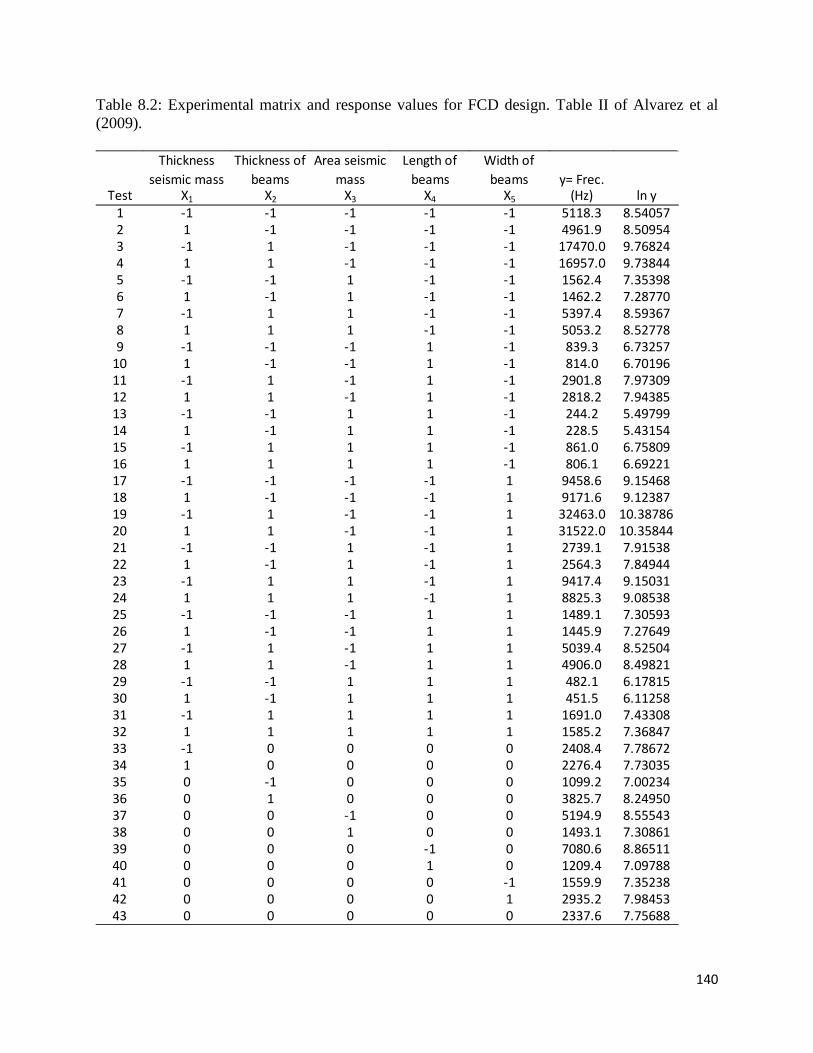
140
Table 8.2: Experimental matrix and response values for FCD design. Table II of Alvarez et al (2009).
Thickness seismic mass
Thickness of beams
Area seismic mass
Length of beams
Width of beams y= Frec.
Test X1 X2 X3 X4 X5 (Hz) ln y1 -1 -1 -1 -1 -1 5118.3 8.540572 1 -1 -1 -1 -1 4961.9 8.509543 -1 1 -1 -1 -1 17470.0 9.768244 1 1 -1 -1 -1 16957.0 9.738445 -1 -1 1 -1 -1 1562.4 7.353986 1 -1 1 -1 -1 1462.2 7.287707 -1 1 1 -1 -1 5397.4 8.593678 1 1 1 -1 -1 5053.2 8.527789 -1 -1 -1 1 -1 839.3 6.73257
10 1 -1 -1 1 -1 814.0 6.7019611 -1 1 -1 1 -1 2901.8 7.9730912 1 1 -1 1 -1 2818.2 7.9438513 -1 -1 1 1 -1 244.2 5.4979914 1 -1 1 1 -1 228.5 5.4315415 -1 1 1 1 -1 861.0 6.7580916 1 1 1 1 -1 806.1 6.6922117 -1 -1 -1 -1 1 9458.6 9.1546818 1 -1 -1 -1 1 9171.6 9.1238719 -1 1 -1 -1 1 32463.0 10.3878620 1 1 -1 -1 1 31522.0 10.3584421 -1 -1 1 -1 1 2739.1 7.9153822 1 -1 1 -1 1 2564.3 7.8494423 -1 1 1 -1 1 9417.4 9.1503124 1 1 1 -1 1 8825.3 9.0853825 -1 -1 -1 1 1 1489.1 7.3059326 1 -1 -1 1 1 1445.9 7.2764927 -1 1 -1 1 1 5039.4 8.5250428 1 1 -1 1 1 4906.0 8.4982129 -1 -1 1 1 1 482.1 6.1781530 1 -1 1 1 1 451.5 6.1125831 -1 1 1 1 1 1691.0 7.4330832 1 1 1 1 1 1585.2 7.3684733 -1 0 0 0 0 2408.4 7.7867234 1 0 0 0 0 2276.4 7.7303535 0 -1 0 0 0 1099.2 7.0023436 0 1 0 0 0 3825.7 8.2495037 0 0 -1 0 0 5194.9 8.5554338 0 0 1 0 0 1493.1 7.3086139 0 0 0 -1 0 7080.6 8.8651140 0 0 0 1 0 1209.4 7.0978841 0 0 0 0 -1 1559.9 7.3523842 0 0 0 0 1 2935.2 7.9845343 0 0 0 0 0 2337.6 7.75688

141
The estimated regression coefficients and statistical significance of a full quadratic model were shown in Table III of the paper and are reproduced here as Table 8.3. The polynomial prediction equation in coded factors for the logarithm of the natural frequency using only statistically significant terms at the 5% level was given as:
ln y = 7.7587 − 0.02409 𝑥𝑥1 + 0.61991 𝑥𝑥2 − 0.60441 𝑥𝑥3 − 0.90245 𝑥𝑥4 + 0.30307 𝑥𝑥5− 0.13301 𝑥𝑥22 + 0.17309 𝑥𝑥32 + 0.22256 𝑥𝑥42 − 0.0948 𝑥𝑥52 + 0.0104 𝑥𝑥3 𝑥𝑥4
The model has an adjusted R2 of 0.999, and all regression assumptions were checked and fulfilled.
Table 8.3: Estimated regression coefficients. Table III of Alvarez et al (2009).
The ANOVA results, showing the contribution of the various order of terms, considering only the statistically significant terms, were shown in Table IV of the paper. The table is reproduced here as Table 8.4.
Coeff SE coeff T PConstant 7.75870 0.01033 751.457 0.000
x1 Thickness of seismic mass -0.02409 0.00479 -5.029 0.000x2 Thickness of beams 0.61991 0.00479 129.389 0.000x3 Area of seismic mass -0.60441 0.00479 -126.154 0.000x4 Length of beams -0.90245 0.00479 -188.362 0.000x5 Width of beams 0.30307 0.00479 63.257 0.000x1
2 Thickness of mass x thickness of mass -0.00040 0.01783 -0.022 0.982x2
2 Thickness of beams x thickness of beams 0.13301 0.01783 -7.461 0.000x3
2 Area seismic mass x area seismic mass 0.17309 0.01783 9.709 0.000x4
2 Length of beams x length of beams 0.22256 0.01783 12.484 0.000x5
2 Width of beams x width of beams -0.09048 0.01783 -5.075 0.000x1x2 Thickness s. mass x thickness of beams 0.00030 0.00494 0.060 0.952x1x3 Thickness of s. mass x area seismic mass -0.00901 0.00494 -1.825 0.082x1x4 Thickness of s. mass x thickness of beams 0.00017 0.00494 0.035 0.973x1x5 Thickness of s. mass x width of beams 0.00024 0.00494 0.048 0.962x2x3 Thickness of beams x area seismic beams 0.00421 0.00494 0.852 0.403x2x4 Thickness of beams x length of beams 0.00250 0.00494 0.506 0.618x2x5 Thickness of beams x width of beams -0.00154 0.00494 -0.312 0.758x3x4 Area of seismic mass x length of beams 0.01040 0.00494 2.107 0.047x3x5 Area of sesmic mass x width of beams 0.00711 0.00494 1.440 0.164x4x5 Length of beams x width of beams 0.00816 0.00494 1.653 0.113
Term

142
Table 8.4: Analysis of variance for ln y. Table IV of Alvarez et al (2009).
From Table 8.4, it shows that linear terms have more significant contribution than quadratic terms, and interaction terms have the least contribution. Furthermore, among the five factors, the seismic mass has the lowest influence on the natural frequency.
The authors did not provide any additional experimental runs that were not used for model development, to verify the model.
Case Study #8.2
Chiang, Ko-Ta, and Fu-Ping Chang (2006): Application of response surface methodology in the parametric optimization of a pin-fin type heat sink. International Communications in Heat and Mass Transfer, 33, pp. 836-845.
This study used response surface methodology to find optimal values for the design parameters of a pin-fin type heat sink (PFHS) to achieve high thermal performance (or cooling efficiency). These heat sinks are widely used to provide cooling of electronic components. Experiments were performed using a face-centered central composite design (FCD) with four factors. The factors and levels used in the experiment were given in Table 1 of the paper and are shown here in Table 8.5.
Table 8.5: Design scheme of designing parameters and their levels. Table 1 of Chiang et al (2006).
The two responses of relevance in this experiment were the thermal resistance, Rth (°C/W) and pressure drop, ∆P (Pa). The design and other technical details of the heat sink were described in detail in the paper.
Source DF Seq SS Adj SS Adj MS F PRegression 10 56.6842 56.6842 5.6684 7443.81 0.000Linear 5 56.3190 56.3190 11.2638 14791.72 0.000Square 4 0.3617 0.3617 0.0904 118.74 0.000Interaction 1 0.0035 0.0035 0.0035 4.55 0.041Residual error 32 0.0244 0.0244 0.0008Total 42R2 = 0.999
Symbol Factor Unit Low (-1) High (+1)A Fin Height, H mm 50 60B Pin diameter, D mm 4 6C Longitudinal pitch, S1 mm 6 10D Transverse pitch, S2 mm 8 12
Levels

143
The FCD had a total of 30 experimental runs (16 factorial points, eight axial points, and six center points). The experimental design and measured responses were given in Table 2 of the paper and are reproduced here as Table 8.6. The software used for the design and analysis of the experiment was not mentioned.
Table 8.6: Design of experimental matrix and results for the PFHS performance characteristics. Table 2 of Chiang et al (2006).
The authors fitted a second-order polynomial regression model to each of the responses. The full ANOVA results including all terms in the models were given in Tables 3 and 5 of the paper for the thermal resistance and pressure drop, respectively. The authors also showed ANOVA tables resulting from using the backward elimination procedure to reduce the model. These reduced ANOVA tables for thermal resistance and pressure drop were shown as Tables 4 and 6 in the paper and are reproduced here as Tables 8.7 and 8.8, respectively. It is of interest to note that after using backward elimination, there are still statistically insignificant terms left in the ANOVA tables. It is also likely that statistically significant terms have been incorrectly left out of the tables. Hence the models developed by the authors may not be the best models.
Exp No. (A) Fin height (B) Pin diameter (C) Long. Pitch (D) Trans. Pitch Therm resist, Rth (°C/W) Pressure drop, ∆P (Pa)1 50 4 6 8 0.258 28.32 60 4 6 8 0.213 23.83 50 6 6 8 0.243 26.84 60 6 6 8 0.201 22.65 50 4 10 8 0.241 26.66 60 4 10 8 0.198 22.37 50 6 10 8 0.217 24.28 60 6 10 8 0.193 21.89 50 4 6 12 0.235 26.210 60 4 6 12 0.204 22.911 50 6 6 12 0.231 25.612 60 6 6 12 0.201 20.913 50 4 10 12 0.236 26.114 60 4 10 12 0.198 21.815 50 6 10 12 0.212 23.716 60 6 10 12 0.189 21.417 50 5 8 10 0.231 25.618 60 5 8 10 0.203 22.819 55 4 8 10 0.224 24.920 55 6 8 10 0.211 23.621 55 5 6 10 0.235 25.222 55 5 10 10 0.214 23.923 55 5 8 8 0.223 24.824 55 5 8 12 0.218 23.725 55 5 8 10 0.224 24.826 55 5 8 10 0.232 24.627 55 5 8 10 0.223 25.128 55 5 8 10 0.222 24.729 55 5 8 10 0.227 24.430 55 5 8 10 0.223 24.5
Design parameters Experimental results

144
Table 8.7: ANOVA table for the thermal resistance (after backward elimination). Table 4 of Chiang et al (2006).
Table 8.8: ANOVA table for the pressure drop (after backward elimination). Table 6 of Chiang et al (2006).
From Table 8.7, the final response equations for thermal resistance in terms of coded and actual factors were given as Equations 5 and 6, respectively, in the paper. They are reproduced here below:
Source Sum of squares DF Mean square f-value Prob>FModel 0.00694 5 0.001389 40.3058 <0.0001 SignificantA 0.00513 1 0.005134 148.9730 <0.0001B 0.00066 1 0.000660 19.1520 0.0002C 0.00084 1 0.000841 24.3877 <0.0001D 0.000221 1 0.000221 6.3980 0.0184AB 9.03E-05 1 9.03E-05 2.6187 0.1187Residual 0.000827 24 3.45E-05Lack of fit 0.000756 19 3.98E-05 2.8098 0.1279 Not significantPure error 7.083E-05 5 1.42E-05Cor. Total 0.007772 29Standard deviation = 0.005870 R2 = 0.89358Mean = 0.219333 R2 adjusted = 0.87141Coefficient of variation = 2.676572 Predicted R2 = 0.82395PRESS = 0.001368 Adequate precision = 25.3505
Source Sum of squares DF Mean square f-value Prob>FModel 79.69944 5 15.93988 65.7850 <0.0001 SignificantA 59.76888 1 59.76888 246.6720 <0.0001B 8.405 1 8.40500 34.6880 <0.0001C 6.12500 1 6.12500 25.2780 <0.0001D 4.40055 1 4.40055 18.1610 0.0003CD 1.00E+00 1 1.00000 4.1270 0.0534Residual 5.81522 24 0.24230Lack of fit 5.506888 19 0.28984 4.7000 0.0572 Not significantPure error 0.308330 5 0.061666Cor. Total 85.512466 29Standard deviation = 0.492240 R2 = 0.93199Mean = 24.253333 R2 adjusted = 0.91783Coefficient of variation = 2.029579 Predicted R2 = 0.87782PRESS = 10.447778 Adequate precision = 32.55552

145
Coded factors:
Thermal resistance = 0.2193 – 0.0169 A – 0.0061 B – 0.0068 C – 0.0035 D + 0.0024 AB
Actual factors:
Thermal resistance = 0.6108 – 0.0058 H – 0.0322 D – 0.0034 S1 – 0.0018 S2 + 0.0005 HD.
From Table 8.8, the final response equations for pressure drop in terms of coded and actual factors were given as Equations 7 and 8, respectively, in the paper. These equations are reproduced below:
Coded factors:
Pressure drop = 24.2533 – 1.8222 A – 0.6833 B – 0.5833 C – 0.4944 D + 0.25 CD
Actual factors:
Pressure drop = 57.52 – 0.3644 H – 0.6833 D – 0.9166 S1 – 0.7472 S2 + 0.0625 S2.
The authors then went on to find the optimal values for the fin parameters [H, D, S1, S2] to minimize thermal resistance and pressure drop using a sequential approximation optimization method. They also set the constraints for the parameters as: 50 ≤ H ≤ 60 mm, D ≤ 6 mm, 6 ≤ S1 ≤ 8, 8 ≤ S2 ≤ 12 mm, and mass of the PFHS ≤ 620 g.
The optimal settings obtained were shown in Table 7 of the paper and are shown here as Table 8.9.
Table 8.9: The optimal designing parameters. Table 7 of Chiang et al (2006).
To verify the adequacy of the developed models, three confirmation runs were performed. The results obtained for the thermal resistance and pressure drop using the regression models were then compared to those obtained experimentally. These comparisons were shown in Table 8 of the paper and are reproduced here as Table 8.10. However, no confirmation runs were done at the optimal settings.
Parameters Unit Optimal valueFin height, H mm 60Pin diameter, D mm 4.76Longitudinal pitch, S1 mm 10Transverse pitch, S2 mm 11.96Predicted valueThermal resistance, Rth °C/W 0.192Pressure drop, ∆P Pa 21.71

146
Table 8.10: Confirmation experiments. Table 8 of Chiang et al (2006).
Based on the confirmation runs, the authors concluded that the developed models were accurate, even though no confirmation runs were performed at the optimal settings.
Case Study #8.3
Jenarthanan, M. P. and R. Jeyapaul (2014): Machinability study of carbon fibre reinforced polymer (CFRP) composites using design of experiment technique. Pigment & Resin Technology, 43/1, pp. 35-44.
This study investigated the influence of three input CNC machining parameters on the surface delamination of carbon fibre reinforced polymer (CFRP) when milled by a machine with a solid carbide end mill coated with crystalline diamond. The input parameters were the cutting speed, feed rate, and depth of cut. A second-order response surface model based on a face-centred central composite design (FCD) was used. The FCD had eight factorial points, six axial points, and six center points giving a total of 20 run combinations. The response measured was the delamination factor, Fd. The materials and experimental procedure used were described in the paper. The factors and their levels used were given in Table II of the paper and are reproduced here as Table 8.11.
Table 8.11: Process control parameters and their levels. Table II of Jenarthanan et al (2014).
The design and analysis of the experimental data were carried out using Design-Expert 8.0 software. The experimental layout in coded and actual factors and the results were shown in Table III of the paper and are reproduced here as Table 8.12.
The authors fitted a full second-order (main effects, two-factor interactions, and quadratic terms) model to the responses. The ANOVA results were shown in Table IV of the paper and are shown here as Table 8.13.
Exp No.A B C D Exp. Predicted Error (%) Exp. Predicted Error (%)
1 50 4 6 12 0.235 0.247 -5.11 26.2 26.5 -1.152 55 5 8 10 0.224 0.219 2.23 24.8 24.2 2.423 60 6 10 8 0.193 0.202 4.66 21.8 22.7 -4.13
Designing parameters Pressure drop, ∆PThermal resistance, Rth
Process parameters Units Notattion Variable -1 0 1Feed rate mm/rev f A 0.04 0.08 0.12Cutting speed m/min V B 50 75 100Depth of cut mm D C 0.05 0.15 0.25
Levels

147
Table 8.12: Layout of full factorial face-centred central composite design with results. Table III of Jenarthanan et al (2014).
Table 8.13: ANOVA for delamination. Table IV of Jenarthanan et al (2014).
Delamination factorRun A B C f V D Fd
1 0 0 0 0.08 75 0.15 1.02092 -1 -1 -1 0.04 50 0.05 1.01133 1 0 0 0.12 75 0.15 1.05374 1 1 1 0.12 100 0.25 1.06545 1 -1 -1 0.12 50 0.05 1.04266 0 0 0 0.08 75 0.15 1.03197 -1 -1 1 0.04 50 0.25 1.00638 0 0 1 0.08 75 0.25 1.03379 0 0 -1 0.08 75 0.05 1.023810 -1 1 -1 0.04 100 0.05 1.005111 0 1 0 0.08 100 0.15 1.040812 1 -1 1 0.12 50 0.25 1.043613 0 0 0 0.08 75 0.15 1.031914 -1 1 1 0.04 100 0.25 1.018615 1 1 -1 0.12 100 0.05 1.057916 0 0 0 0.08 75 0.15 1.031917 0 0 0 0.08 75 0.15 1.031918 0 -1 0 0.08 50 0.15 1.025819 0 0 0 0.08 75 0.15 1.031920 -1 0 0 0.04 75 0.15 1.0055
Coded variables Uncoded variables
Source Sum of squares df Mean squares F-value p-value Effect % contributionModel 5.533 x 10-03 9 6.148 x 10-04 386.5 <0.0001 Significant 99.71A 4.844 x 10-03 1 4.844 x 10-03 3045.7 <0.0001 Significant 87.28B 5.314 x 10-04 1 5.314 x 10-04 334.1 <0.0001 Significant 9.56C 1.129 x 10-04 1 1.129 x 10-04 71 <0.0001 Significant 2.03AB 4.961 x 10-06 1 4.961 x 10-06 3.1 0.1078 Insignificant 0.08AC 6.661 x 10-06 1 6.661 x 10-06 4.2 0.0679 Insignificant 0.11BC 3.612 x 10-07 1 3.612 x 10-07 0.2 0.6439 Insignificant 0.00A2 1.903 x 10-06 1 1.903 x 10-06 1.2 0.2997 Insignificant 0.03B2 3.120 x 10-05 1 3.120 x 10-05 19.6 0.0013 Significant 0.55C2 3.841 x 10-06 1 3.841 x 10-06 2.4 0.1512 Insignificant 0.07Error 1.591 x 10-05 10 1.591 x 10-06 Insignificant 0.29Total 5.549 x 10-03 19Notes: R2 = 99.91; adjusted R2 = 99.46

148
From Table 8.13, many of the model terms were not statistically significant at the 5% level. Only the main effects A, B, C, and the quadratic term B2 were statistically significant. However, the authors suggested a final model with all terms regardless of statistical significance. The final model in terms of coded factors was:
Delamination Factor (Fd) = 1.03 + 0.022 A + 7.290 x 10-03 B + 3.360 x 10-03 C + 7.875 x 10-04 AB + 9.125 x 10-04 AC – 2.125 x 10-04 BC – 8.318 x 10-04 A2 + 3.368 x 10-03 B2 – 1.182 x 10-03 C2
And, the final model in terms of actual factors was:
Delamination Factor (Fd) = 0.99042 + 0.54015 feedrate – 5.67014 x 10-04 cuttingspeed + 0.057180 depthofcut + 7.87500 x 10-04 feedrate x cuttingspeed + 0.22813 feedrate x depthofcut – 8.5000 x 10-05 cuttingspeed x depthofcut + 5.38909 x 10-06 (cuttingspeed)2 – 0.11818 (depthofcut)2 There is a squared term (feedrate)2 missing from the model with actual factors. This term may have been accidentally left out by the authors.
The adjusted R2 for the model was 99.46 which was an excellent fit to the data. The authors also ran 20 additional confirmation experiments to validate the model. The results from experiments were compared those obtained from the regression model. These comparison results were shown in Table VI of the paper. The error was found to be within ±0.3 percent. Since the factor settings were not given, it is not possible to reproduce the results shown here.
Reanalyses of the published data using both Design-Expert 12 and Minitab 18 did not reproduce the results reported by the authors. Some of the F-values differed by a factor of 10. Hence, it is possible the ANOVA results shown were incorrect. If this is so, then the models developed were also incorrect.
Case Study #8.4
Kwon, J-H, Sang-Moon Hwang, Chang-Min Lee, Kwang-Suk Kim, and Gun-Yong Hwang (2009): Application of response surface methodology (RSM) in microspeaker design used in mobile phones. IEEE Transactions on Magnetics, Vol. 45, N. 10, pp. 4550-4553.
This study investigated the design of a microspeaker used in mobile phones using response surface methodology based on a face-centered central composite design. The parameters that influence a magnetic circuit design of the microspeaker included the dimensions of the top plate, yoke, and radius of the inner magnet. The design drawing and constraints were given in the paper. The factors and levels used in the study are summarized in Table 8.14. The responses were the mean and variance of the electromagnetic force obtained using finite element analysis. Hence this is a

149
computer based experiment. The goal was to design a microspeaker with a high mean electromagnetic force but with minimum variance.
Table 8.14: Factors and levels used in the experiment.
The authors used a three-factor full-factorial face-centered central composite design (FCD) with eight factorial points, six axial points, and one center point (total of 15 run combinations). The FCD design together with the mean and variance of the electromagnetic force were given in Table 1 of the paper and are reproduced here as Table 8.15.
Table 8.15: Experimental design matrix and results. Table 1 of Kwon et al (2009).
Full second-order regression models were fitted to the two responses. No ANOVA results were given in the paper. Only the fitted regression models in terms of coded factors for the mean and variance of the electromagnetic force were shown (Equation 4 and 5, respectively). These equations are:
𝐹𝐹𝑚𝑚𝑚𝑚𝑚𝑚𝑚𝑚 = 49.4 − 0.03 𝑥𝑥1 + 0.66 𝑥𝑥2 − 0.83 𝑥𝑥3 − 1.25 x12 − 0.10 x22 − 1.85 x32 + 0.075 x1x2− 0.675 x1x3 + 0.15 x2𝑥𝑥3
𝐹𝐹𝑣𝑣𝑚𝑚𝑣𝑣𝑣𝑣𝑚𝑚𝑚𝑚𝑣𝑣𝑚𝑚 = 24.98 + 15.04 𝑥𝑥1 + 0.66 𝑥𝑥2 + 8.12 𝑥𝑥3 + 5.38 x12 − 0.62 x22 − 0.32 x32+ 0.4125 x1x2 + 9.3875 x1x3 + 0.4625 x2𝑥𝑥3
Factor Description Unit -1 0 1x1 Radius of inner magnet mm 3.3 3.8 4.3x2 Thickness of yoke mm 0.2 0.3 0.4x3 Thickness of top plate mm 0.2 0.3 0.4
Levels
Std Ord x1 x2 x3 Mean (mN) Variance {x10-6)1 -1 -1 -1 45.9 16.62 1 -1 -1 47.1 26.53 -1 1 -1 46.8 17.34 1 1 -1 48.3 27.05 -1 -1 1 45.3 12.96 1 -1 1 43.8 58.57 -1 1 1 46.8 13.68 1 1 1 45.6 62.79 -1 0 0 48.3 12.410 1 0 0 48.0 48.511 0 -1 0 48.7 24.212 0 1 0 49.9 24.713 0 0 -1 48.4 14.314 0 0 1 46.7 35.215 0 0 0 49.4 24.6
ResponsesCoded factors
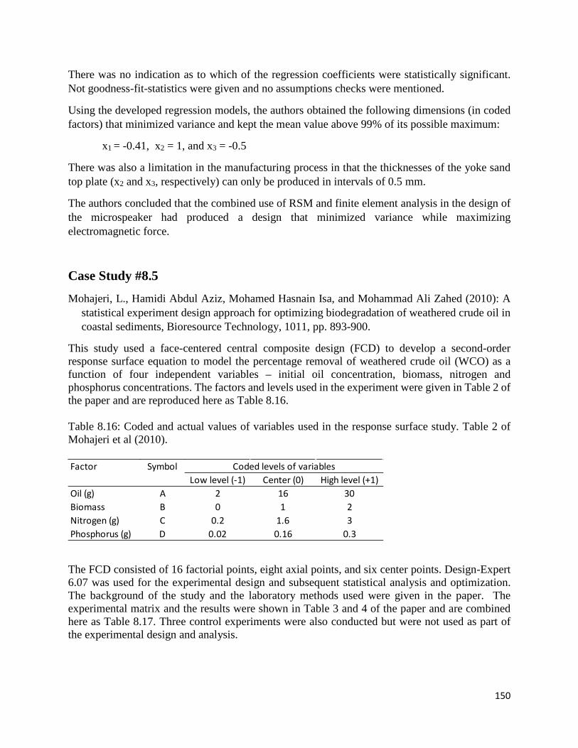
150
There was no indication as to which of the regression coefficients were statistically significant. Not goodness-fit-statistics were given and no assumptions checks were mentioned.
Using the developed regression models, the authors obtained the following dimensions (in coded factors) that minimized variance and kept the mean value above 99% of its possible maximum:
x1 = -0.41, x2 = 1, and x3 = -0.5
There was also a limitation in the manufacturing process in that the thicknesses of the yoke sand top plate (x2 and x3, respectively) can only be produced in intervals of 0.5 mm.
The authors concluded that the combined use of RSM and finite element analysis in the design of the microspeaker had produced a design that minimized variance while maximizing electromagnetic force.
Case Study #8.5
Mohajeri, L., Hamidi Abdul Aziz, Mohamed Hasnain Isa, and Mohammad Ali Zahed (2010): A statistical experiment design approach for optimizing biodegradation of weathered crude oil in coastal sediments, Bioresource Technology, 1011, pp. 893-900.
This study used a face-centered central composite design (FCD) to develop a second-order response surface equation to model the percentage removal of weathered crude oil (WCO) as a function of four independent variables – initial oil concentration, biomass, nitrogen and phosphorus concentrations. The factors and levels used in the experiment were given in Table 2 of the paper and are reproduced here as Table 8.16. Table 8.16: Coded and actual values of variables used in the response surface study. Table 2 of Mohajeri et al (2010).
The FCD consisted of 16 factorial points, eight axial points, and six center points. Design-Expert 6.07 was used for the experimental design and subsequent statistical analysis and optimization. The background of the study and the laboratory methods used were given in the paper. The experimental matrix and the results were shown in Table 3 and 4 of the paper and are combined here as Table 8.17. Three control experiments were also conducted but were not used as part of the experimental design and analysis.
Factor SymbolLow level (-1) Center (0) High level (+1)
Oil (g) A 2 16 30Biomass B 0 1 2Nitrogen (g) C 0.2 1.6 3Phosphorus (g) D 0.02 0.16 0.3
Coded levels of variables
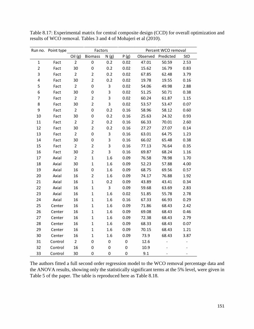
151
Table 8.17: Experimental matrix for central composite design (CCD) for overall optimization and results of WCO removal. Tables 3 and 4 of Mohajeri et al (2010).
The authors fitted a full second order regression model to the WCO removal percentage data and the ANOVA results, showing only the statistically significant terms at the 5% level, were given in Table 5 of the paper. The table is reproduced here as Table 8.18.
Run no. Point typeOil (g) Biomass N (g) P (g) Observed Predicted StD
1 Fact 2 0 0.2 0.02 47.01 50.59 2.532 Fact 30 0 0.2 0.02 15.62 16.79 0.833 Fact 2 2 0.2 0.02 67.85 62.48 3.794 Fact 30 2 0.2 0.02 19.78 19.55 0.165 Fact 2 0 3 0.02 54.06 49.98 2.886 Fact 30 0 3 0.02 51.25 50.71 0.387 Fact 2 2 3 0.02 60.24 61.87 1.158 Fact 30 2 3 0.02 53.57 53.47 0.079 Fact 2 0 0.2 0.16 58.96 58.12 0.60
10 Fact 30 0 0.2 0.16 25.63 24.32 0.9311 Fact 2 2 0.2 0.16 66.33 70.01 2.6012 Fact 30 2 0.2 0.16 27.27 27.07 0.1413 Fact 2 0 3 0.16 63.01 64.75 1.2314 Fact 30 0 3 0.16 66.02 65.48 0.3815 Fact 2 2 3 0.16 77.13 76.64 0.3516 Fact 30 2 3 0.16 69.87 68.24 1.1617 Axial 2 1 1.6 0.09 76.58 78.98 1.7018 Axial 30 1 1.6 0.09 52.23 57.88 4.0019 Axial 16 0 1.6 0.09 68.75 69.56 0.5720 Axial 16 2 1.6 0.09 74.17 76.88 1.9221 Axial 16 1 0.2 0.09 43.89 43.41 0.3422 Axial 16 1 3 0.09 59.68 63.69 2.8323 Axial 16 1 1.6 0.02 51.85 55.78 2.7824 Axial 16 1 1.6 0.16 67.33 66.93 0.2925 Center 16 1 1.6 0.09 71.86 68.43 2.4226 Center 16 1 1.6 0.09 69.08 68.43 0.4627 Center 16 1 1.6 0.09 72.38 68.43 2.7928 Center 16 1 1.6 0.09 68.33 68.43 0.0729 Center 16 1 1.6 0.09 70.15 68.43 1.2130 Center 16 1 1.6 0.09 73.9 68.43 3.8731 Control 2 0 0 0 12.6 - -32 Control 16 0 0 0 10.9 - -33 Control 30 0 0 0 9.1 - -
Percent WCO removalFactors

152
Table 8.18: Analysis of variance for response surface quadratic model terms. Table 5 of Mohajeri et al (2010).
The regression model based on only statistically significant terms is given by (Equation 3 in the paper):
WCO removal (percent) = 68.43 – 10.55 A + 3.66 B + 10.14 C + 5.57 D + 4.79 B2 – 14.89 C2 – 7.08D2 – 2.28 AB + 8.63 AC + 1.81 CD The model has a R2 of 0.9732, adjusted R2 of 0.9591, and predicted R2 of 0.9336. The interpretation of the interaction terms were given in the paper. The authors used the developed regression model to obtain factor settings to maximize WCO removal for initial oil concentrations of 2, 16, and 30 g/kg. The results comparing observed and predicted values were given in Table 6 of the paper and are reproduced here as Table 8.19. Table 8.19: Optimum conditions found by Design-Expert for the WCO bioremediation. Table 6 of Mohajeri et al (2010).
The authors also compared the unoptimized values at for 2, 16, and 30 g/kg (77.13%, 74.17%, and 69.87%, respectively) of initial oil concentration with the optimized values (83.13%, 78.06%, and 69.92%, respectively).
Source Sum of Squares df Mean Square F-value p-value RemarksModel 8106.65 10 810.67 69.04 < 0.0001 significantA-A 2004.08 1 2004.08 170.68 < 0.0001 significantB-B 241.27 1 241.27 20.55 0.0002 significantC-C 1850.14 1 1850.14 157.57 < 0.0001 significantD-D 559.12 1 559.12 47.62 < 0.0001 significantB² 65.1 1 65.1 5.54 0.0294 significantC² 629.04 1 629.04 53.57 < 0.0001 significantD² 142.34 1 142.34 12.12 0.0025 significantAB 83.45 1 83.45 7.11 0.0153 significantAC 1192.32 1 1192.32 101.55 < 0.0001 significantCD 52.49 1 52.49 4.47 0.0479 significantResidual 223.09 19 11.74Lack of Fit 200.51 14 14.32 3.17 0.1044 not significantPure Error 22.58 5 4.52Cor Total 8329.74 29
Oil (g) Biomass N (g) P (g) Observed Predicted Percent error StD2 2 0.680 0.140 83.13 85.01 -2.26 1.3316 2 2.164 0.231 78.06 80.59 -3.24 1.7930 2 2.520 0.250 69.92 71.54 -2.32 1.15
WCO percent removal

153
Case Study #8.6
Noordin, M. Y., V.C. Venkatesh, S. Sharif, S. Elting, and A. Abdullah (2004): Application of response surface methodology in describing the performance of coated carbide tools when turning AISI 1045 steel. Journal of Materials Processing Technology, 145, pp. 46-58.
This study investigated the factors that influence the surface roughness and tangential force of a multilayer tungsten carbide tool when turning AISI 1045 steel. The factors investigated were the cutting speed, feed, and the side cutting edge angle (SCEA) of the cutting edge. The experiments were based on a face-centered central composite design (FCD). The factors and levels used in the experiment were shown in Table 1 of the paper and are reproduced here as Table 8.20. Table 8.20: Factors and levels for response surface study. Table 1 of Noordin et al (2004).
The FCD consisted of 16 experimental points (eight factorial points, six axial points, and two center points). The responses measured were the surface roughness, Ra (µ) of the turned surface, and the main cutting force, i.e. the tangential force, Fc (N). The experimental design and results were shown in Tables 2 and 3 of the paper. The tables are combined here as Table 8.21.
Table 8.21: Completed design layout and experimental results. (Tables 2 and 3 of Noordin et al (2004).
Factor Low level (-1) High Level (+1)A - cutting speed (m/min) 240 375B - feed (mm/rev) 0.18 0.28C - SCEA (°) -5 0
Std No. Run A-cutting B - feed C - SCEA Surface Tangentialspeed (m/min) (mm/rev) (°) roughness, Ra (µ) force, Fc (N)
1 8 240 0.18 -5 1.68 395.982 9 375 0.18 -5 1.40 372.243 12 240 0.28 -5 3.18 550.144 15 375 0.28 -5 2.95 525.855 13 240 0.18 0 1.20 372.836 3 375 0.18 0 1.42 366.487 11 240 0.28 0 3.80 559.228 2 375 0.28 0 3.25 553.509 14 240 0.23 -3 2.14 443.1010 16 375 0.23 -3 2.08 432.2711 6 300 0.18 -3 1.14 351.1412 7 300 0.28 -3 2.99 540.7713 1 300 0.23 -5 2.17 440.9214 4 300 0.23 0 2.32 465.4015 10 300 0.23 -3 1.76 436.1016 5 300 0.23 -3 1.74 428.88
Factor
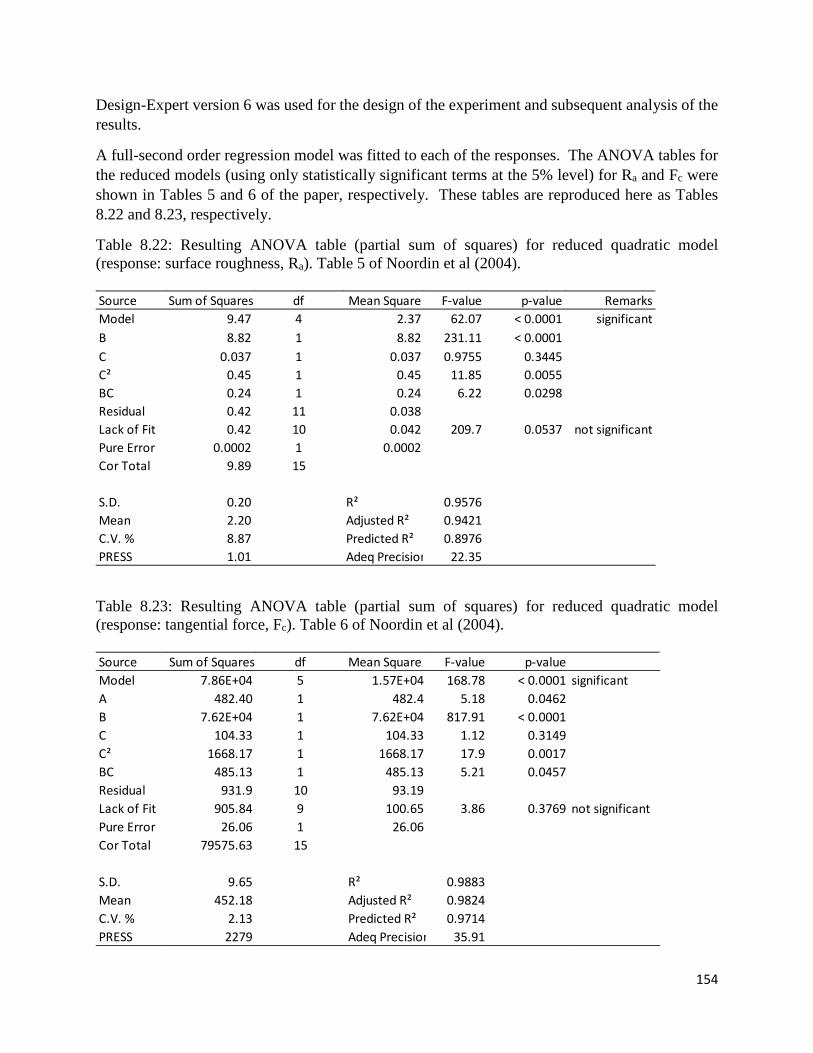
154
Design-Expert version 6 was used for the design of the experiment and subsequent analysis of the results.
A full-second order regression model was fitted to each of the responses. The ANOVA tables for the reduced models (using only statistically significant terms at the 5% level) for Ra and Fc were shown in Tables 5 and 6 of the paper, respectively. These tables are reproduced here as Tables 8.22 and 8.23, respectively.
Table 8.22: Resulting ANOVA table (partial sum of squares) for reduced quadratic model (response: surface roughness, Ra). Table 5 of Noordin et al (2004).
Table 8.23: Resulting ANOVA table (partial sum of squares) for reduced quadratic model (response: tangential force, Fc). Table 6 of Noordin et al (2004).
Source Sum of Squares df Mean Square F-value p-value RemarksModel 9.47 4 2.37 62.07 < 0.0001 significantB 8.82 1 8.82 231.11 < 0.0001C 0.037 1 0.037 0.9755 0.3445C² 0.45 1 0.45 11.85 0.0055BC 0.24 1 0.24 6.22 0.0298Residual 0.42 11 0.038Lack of Fit 0.42 10 0.042 209.7 0.0537 not significantPure Error 0.0002 1 0.0002Cor Total 9.89 15
S.D. 0.20 R² 0.9576Mean 2.20 Adjusted R² 0.9421C.V. % 8.87 Predicted R² 0.8976PRESS 1.01 Adeq Precision 22.35
Source Sum of Squares df Mean Square F-value p-valueModel 7.86E+04 5 1.57E+04 168.78 < 0.0001 significantA 482.40 1 482.4 5.18 0.0462B 7.62E+04 1 7.62E+04 817.91 < 0.0001C 104.33 1 104.33 1.12 0.3149C² 1668.17 1 1668.17 17.9 0.0017BC 485.13 1 485.13 5.21 0.0457Residual 931.9 10 93.19Lack of Fit 905.84 9 100.65 3.86 0.3769 not significantPure Error 26.06 1 26.06Cor Total 79575.63 15
S.D. 9.65 R² 0.9883Mean 452.18 Adjusted R² 0.9824C.V. % 2.13 Predicted R² 0.9714PRESS 2279 Adeq Precision 35.91
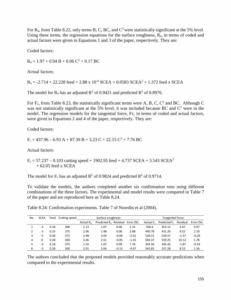
155
For Ra, from Table 8.22, only terms B, C, BC, and C2 were statistically significant at the 5% level. Using these terms, the regression equations for the surface roughness, Ra, in terms of coded and actual factors were given in Equations 1 and 3 of the paper, respectively. They are: Coded factors: Ra = 1.97 + 0.94 B + 0.06 C2 + 0.17 BC Actual factors: Ra = -2.714 + 22.228 feed + 2.88 x 10⁻⁴ SCEA + 0.0583 SCEA2 + 1.372 feed x SCEA The model for Ra has an adjusted R2 of 0.9421 and predicted R2 of 0.8976. For Fc, from Table 8.23, the statistically significant terms were A, B, C, C2 and BC. Although C was not statistically significant at the 5% level, it was included because BC and C2 were in the model. The regression models for the tangential force, Fc, in terms of coded and actual factors, were given in Equations 2 and 4 of the paper, respectively. They are: Coded factors: Fc = 437.96 – 6.93 A + 87.39 B + 3.23 C + 22.15 C2 + 7.76 BC Actual factors: Fc = 57.237 – 0.103 cutting speed + 1902.95 feed + 4.737 SCEA + 3.543 SCEA2 + 62.05 feed x SCEA The model for Fc has an adjusted R2 of 0.9824 and predicted R2 of 0.9714. To validate the models, the authors completed another six confirmation runs using different combinations of the three factors. The experimental and model results were compared in Table 7 of the paper and are reproduced here as Table 8.24. Table 8.24: Confirmation experiments. Table 7 of Noordin et al (2004).
The authors concluded that the proposed models provided reasonably accurate predictions when compared to the experimental results.
No. SCEA Feed Cutting speedActual Ra Predicted Ra Residual Error (%) Actual Fc Predicted Fc Residual Error (%)
1 -3 0.18 300 1.13 1.07 0.06 5.31 356.6 353.13 3.47 0.972 -3 0.23 375 2.06 1.98 0.08 3.88 440.78 431.26 9.52 2.163 -5 0.28 375 2.98 3.04 -0.06 -2.01 528.21 529.57 -1.37 -0.264 0 0.28 300 3.46 3.51 -0.05 -1.45 569.37 559.25 10.12 1.785 -3 0.18 375 1.16 1.07 0.09 7.76 343.56 345.42 -1.87 -0.546 -5 0.28 300 2.91 3.04 -0.13 -4.47 545.81 537.28 8.53 1.56
Surface roughness Tangential force

156
Case Study #8.7
Qian, Fuping and Mingyao Zhang (2005): Study of the natural vortex length of a cyclone with response surface methodology. Computers and Chemical Engineering, 29, pp. 2155-2162.
This study investigated the natural vortex length, an important parameter of a cyclone, as a function of various geometries of a cyclone using response surface methodology. The natural vortex length of cyclones were obtained by numerical simulations using a commercial computational fluid dynamics (CFD) code, Fluent 6.1. A face-centered central composite design (FCD) was used to obtain the run combinations to fit a second-order regression model to the natural vortex lengths. Five factors, all in dimensionless form, were used in the experiment. The theory behind cyclones and how the dimensionless terms were derived were given in the paper. The factors and levels used in the FCD were shown in Table 1 of the paper and are reproduced here as Table 8.25.
Table 8.25: Low and high level settings of the factors used in the response surface model (Hoekstra, 2000). Table 1 of Qian et al (2005).
In Table 8.25, De is the diameter of the cyclone vortex finder, D is the diameter of the cyclone body, a is the height of the cyclone inlet, b is the width of the cyclone inlet, h is the length of the cyclone cylinder, S is the deepness of the vortex finder insertion, and Re is the well-known dimensionless Reynold’s number. All these terms were described in a schematic drawing of the cyclone in the paper. Dividing by D, all factors involving length become dimensionless. The response was the natural vortex length which was also expressed in dimensionless form as l/D.
Minitab 14 software was used for designing and analysing the data. The FCD had 43 runs in total which consisted of 32 full-factorial points, 10 axial points, and one center point since this was a computer-based experiment with no random errors. The experimental design and results were shown in Table 2 of the paper and are reproduced here as Table 8.26.
The authors fitted a full second-order regression model to the dimensionless vortex length (l/D) data and the breakdown of the analysis of variance in terms of linear, squared, and interaction terms was shown in Table 3 of the paper is shown here as Table 8.27. The estimated regression coefficients and test statistics for the coded factors were shown in Table 4 of the paper. The coefficients in terms of actual factors (uncoded units) were also shown in Table 5 of the paper. These tables are reproduced as Tables 8.28 and 8.29, respectively.
Factor xi XiL XiH
De/D X1 0.30 0.70a/D X2 0.30 0.80b/D X3 0.15 0.35(h-S)/D X4 0.50 2.50ln Re X5 10.2 12.9

157
Table 8.26: Central composite design of Y = l/D. Table 2 of Qian et al (2005).
No. X1 X2 X3 X4 X5 Y1 0.3 0.3 0.15 0.5 10.20 5.0002 0.7 0.3 0.15 0.5 10.20 4.0103 0.3 0.8 0.15 0.5 10.20 4.3004 0.7 0.8 0.15 0.5 10.20 2.9505 0.3 0.3 0.35 0.5 10.20 4.2006 0.7 0.3 0.35 0.5 10.20 3.8507 0.3 0.8 0.35 0.5 10.20 3.5008 0.7 0.8 0.35 0.5 10.20 3.0009 0.3 0.3 0.15 2.5 10.20 4.75010 0.7 0.3 0.15 2.5 10.20 4.50011 0.3 0.8 0.15 2.5 10.20 4.55012 0.7 0.8 0.15 2.5 10.20 4.30013 0.3 0.3 0.35 2.5 10.20 3.95014 0.7 0.3 0.35 2.5 10.20 3.75015 0.3 0.8 0.35 2.5 10.20 4.00016 0.7 0.8 0.35 2.5 10.20 3.80017 0.3 0.3 0.15 0.5 12.90 5.67518 0.7 0.3 0.15 0.5 12.90 4.95019 0.3 0.8 0.15 0.5 12.90 4.95020 0.7 0.8 0.15 0.5 12.90 4.65021 0.3 0.3 0.35 0.5 12.90 5.50022 0.7 0.3 0.35 0.5 12.90 5.30023 0.3 0.8 0.35 0.5 12.90 4.75024 0.7 0.8 0.35 0.5 12.90 4.40025 0.3 0.3 0.15 2.5 12.90 5.60026 0.7 0.3 0.15 2.5 12.90 5.30027 0.3 0.8 0.15 2.5 12.90 5.25028 0.7 0.8 0.15 2.5 12.90 4.50029 0.3 0.3 0.35 2.5 12.90 5.30030 0.7 0.3 0.35 2.5 12.90 4.92531 0.3 0.8 0.35 2.5 12.90 4.85032 0.7 0.8 0.35 2.5 12.90 4.69533 0.5 0.55 0.25 1.5 11.55 5.24034 0.3 0.55 0.25 1.5 11.55 5.15035 0.7 0.55 0.25 1.5 11.55 4.85036 0.5 0.3 0.25 1.5 11.55 5.30037 0.5 0.8 0.25 1.5 11.55 5.10038 0.5 0.55 0.15 1.5 11.55 5.20039 0.5 0.55 0.35 1.5 11.55 4.70040 0.5 0.55 0.25 0.5 11.55 5.25041 0.5 0.55 0.25 2.5 11.55 5.20042 0.5 0.55 0.25 1.5 10.20 4.75043 0.5 0.55 0.25 1.5 12.90 5.650
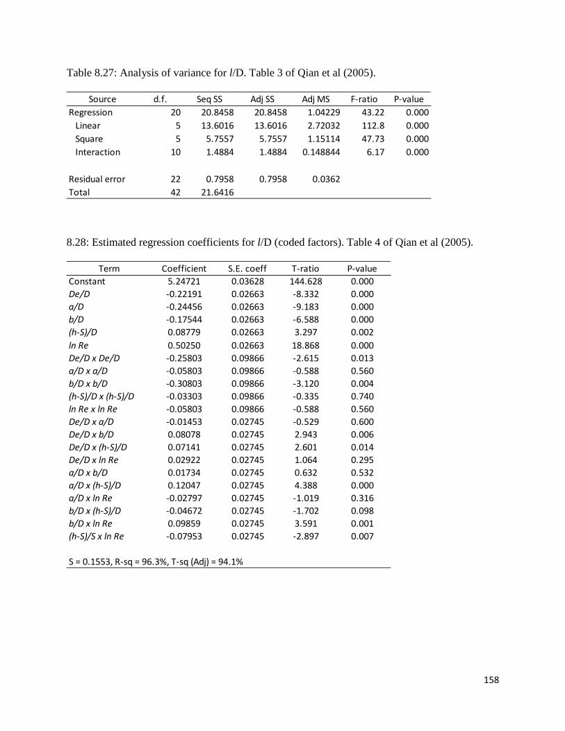
158
Table 8.27: Analysis of variance for l/D. Table 3 of Qian et al (2005).
8.28: Estimated regression coefficients for l/D (coded factors). Table 4 of Qian et al (2005).
Source d.f. Seq SS Adj SS Adj MS F-ratio P-valueRegression 20 20.8458 20.8458 1.04229 43.22 0.000 Linear 5 13.6016 13.6016 2.72032 112.8 0.000 Square 5 5.7557 5.7557 1.15114 47.73 0.000 Interaction 10 1.4884 1.4884 0.148844 6.17 0.000
Residual error 22 0.7958 0.7958 0.0362Total 42 21.6416
Term Coefficient S.E. coeff T-ratio P-valueConstant 5.24721 0.03628 144.628 0.000De/D -0.22191 0.02663 -8.332 0.000a/D -0.24456 0.02663 -9.183 0.000b/D -0.17544 0.02663 -6.588 0.000(h-S)/D 0.08779 0.02663 3.297 0.002ln Re 0.50250 0.02663 18.868 0.000De/D x De/D -0.25803 0.09866 -2.615 0.013a/D x a/D -0.05803 0.09866 -0.588 0.560b/D x b/D -0.30803 0.09866 -3.120 0.004(h-S)/D x (h-S)/D -0.03303 0.09866 -0.335 0.740ln Re x ln Re -0.05803 0.09866 -0.588 0.560De/D x a/D -0.01453 0.02745 -0.529 0.600De/D x b/D 0.08078 0.02745 2.943 0.006De/D x (h-S)/D 0.07141 0.02745 2.601 0.014De/D x ln Re 0.02922 0.02745 1.064 0.295a/D x b/D 0.01734 0.02745 0.632 0.532a/D x (h-S)/D 0.12047 0.02745 4.388 0.000a/D x ln Re -0.02797 0.02745 -1.019 0.316b/D x (h-S)/D -0.04672 0.02745 -1.702 0.098b/D x ln Re 0.09859 0.02745 3.591 0.001(h-S)/S x ln Re -0.07953 0.02745 -2.897 0.007
S = 0.1553, R-sq = 96.3%, T-sq (Adj) = 94.1%

159
The second-order regression model using the coefficients of Table 8.29 was given as Equation 6 of the paper. This equation is:
𝑌𝑌 =𝑙𝑙𝐷𝐷
= −3.59538 + 2.70570 𝑋𝑋1 + 0.249231 𝑋𝑋2 + 3.51131 𝑋𝑋3 + 0.540555 𝑋𝑋4+ 1.00495 𝑋𝑋5 − 6.45064 𝑋𝑋12 − 0.928410 𝑋𝑋22 − 30.8026 𝑋𝑋32 − 0.0330256 𝑋𝑋42− 0.0318385 𝑋𝑋52 − 0.290625 𝑋𝑋1𝑋𝑋2 + 4.03906 𝑋𝑋1𝑋𝑋3 + 0.357031 𝑋𝑋1𝑋𝑋4+ 0.108218 𝑋𝑋1𝑋𝑋5 + 0.693750 𝑋𝑋2𝑋𝑋3 0.481875 𝑋𝑋2𝑋𝑋4 − 0.082870 𝑋𝑋2𝑋𝑋5− 0.0467188 𝑋𝑋3𝑋𝑋4 + 0.730324 𝑋𝑋3𝑋𝑋5 − 0.0589120 𝑋𝑋4𝑋𝑋5
Table 8.29: Estimated regression coefficients for l/D using data in uncoded units. Table 5 of Qian et al (2005).
Term Coefficient Constant -3.595380 De/D 2.705700 a/D 0.249231 b/D 3.511310 (h-S)/D 0.540555 ln Re 1.004950 De/D x De/D -6.450640 a/D x a/D -0.928410 b/D x b/D -30.802600 (h-S)/D x (h-S)/D -0.033026 ln Re x ln Re -0.031839 De/D x a/D -0.290625 De/D x b/D 4.039060 De/D x (h-S)/D 0.357031 De/D x ln Re 0.108218 a/D x b/D 0.693750 a/D x (h-S)/D 0.481875 a/D x ln Re -0.082870 b/D x (h-S)/D -0.467188 b/D x ln Re 0.730324 (h-S)/S x ln Re -0.058912
Attempts to reproduce the exact results obtained in the above tables were not successful using Minitab 18 or Design-Expert 12. The goodness-of-fit obtained using the given data is lower but the statistically significant terms in the quadratic model are similar to those reported by the authors. It seems likely that the analysis by the authors was done using a different set of data than those in Table 8.26. Even if the results were correct, it was not clear why the authors included all terms in the model. Many of the terms were not statistically significant at the 5% level.

160
Case Study #8.8
Sin, H. N., S. Yusof, N. Sheikh Abdul Hamid, and R. Abd. Rahman (2006): Optimization of enzymatic clarification of sapodilla juice using response surface methodology. Journal of Food Engineering, 73, pp. 313-319.
This study investigated the effect of three factors – incubation time, temperature, and enzyme concentration on the enzymatic clarification of sapodilla juice using response surface methodology. Sapodilla, a tropical fruit normally eaten fresh, can be made into a juice but requires the use of enzymes to clarify the juice. The optimal conditions for producing clarified juice was the primary objective of the study.
A face-centered central composite design (FCD) with five center points was used. The factors and levels used in the experiment are summarized in Table 8.30. The materials and methods used in the experiment, including the preparation of the fruit, the extraction of the juice, and the treatment by enzymes, were explained in detail in the paper.
Table 8.30: Factors and levels used in the experiment.
The authors considered four responses as measures of quality of the extracted juice after treatment by the various combinations of the factors. They were the turbidity (NTU), clarity (abs), viscosity (cps), and the colour, based on L values.
The FCD had a total of 19 runs consisting of eight factorial points, six axial points, and five center points. The experiment was run in random order. The 19 run combinations in coded and actual factors, and the results for the four responses, were shown in Table 1 of the paper and are reproduced here as Table 8.31. ECHIP Software Version 6 (Echip Inc., Hockessin, Delaware, USA) was used for the design and analysis of the experiment.
Note that in Table 1 of the paper, all five center points were given the same treatment number of 15. However, it is more conventional to give each treatment combination its own run or treatment number. This was done in Table 8.31. Hence the five center points are labelled as treatment 15, 16, 17, 18, and 19.
The authors fitted a full second-order model (linear, two-factor interaction, and squared terms) to each of the responses. The estimated coefficients, different level of statistical significance, and goodness-of-fit statistics were shown in Table 2 of the paper and are reproduced here as Table 8.32. The coefficients were estimated using actual factors.
Factors Units Low (-1) Center (0) High (+1)Time, X1 min 30 75 120Temperature, X2 °C 30 40 50Enzyme concentration, X3 % 0.03 0.065 0.10
Levels

161
Table 8.31: Effects of incubation time, temperature and enzyme concentration on four dependent variables. Table 1 of Sin et al (2006).
8.32: Regression coefficients and R2 value for four dependent variables for enzymatic clarified sapodilla juices. Table 2 of Sin et al (2006).
Turbidity Clarity Viscosity LTreatment X1 X2 X3 Time (min) Temp. (°C) Enzyme conc. (%) (NTU) (abs) (cps) value
15 0 0 0 75 40 0.065 16.60 0.03 1.39 54.551 -1 0 0 30 40 0.065 34.40 0.03 1.40 52.159 1 -1 1 120 30 0.1 22.30 0.03 1.25 53.77
16 0 0 0 75 40 0.065 16.20 0.02 1.35 54.0110 -1 -1 1 30 30 0.1 19.00 0.02 1.39 53.177 1 1 1 120 50 0.1 18.80 0.01 1.34 54.89
17 0 0 0 75 40 0.065 17.00 0.03 1.40 54.213 0 -1 0 75 30 0.065 18.10 0.03 1.42 54.018 -1 1 1 30 50 0.1 29.90 0.03 1.34 54.00
18 0 0 0 75 40 0.065 15.00 0.02 1.38 54.4212 -1 1 -1 30 50 0.03 65.30 0.07 1.40 49.365 0 0 -1 75 40 0.03 49.70 0.05 1.45 51.73
19 0 0 0 75 40 0.065 14.60 0.03 1.40 54.3811 1 1 -1 120 50 0.03 43.20 0.05 1.39 51.8813 1 -1 -1 120 30 0.03 52.10 0.05 1.43 51.592 1 0 0 120 40 0.065 21.10 0.02 1.28 54.116 0 0 1 75 40 0.1 12.20 0.02 1.25 54.254 0 1 0 75 50 0.065 14.80 0.02 1.41 54.10
14 -1 -1 -1 30 30 0.03 68.90 0.08 1.46 48.10
Indepdent variables Dependent variablesUncoded variablesCoded variables
Regression coefficient Turbidity (NTU) Clarity (abs) Viscosity (cps) L valueb0 16.449484 0.023128 1.377732 54.223608b1 -0.133333* -0.000124** -0.000667*** 0.021022*b2 -0.084000 -0.000315 -0.000700 0.035900***b3 505.714303* -0.534857* -1.600000* 49.771423*b1
2 0.005229* 0.000002 -0.000015 -0.000484**b2
2 -0.007113 0.000031 0.000451 -0.000556b3
2 11256.049479* 10.132549** -16.242336 -914.790594*b12 -0.005472** -0.000004 0.000044 -0.000189b13 2.468254* 0.002548*** -0.007937 -0.358730**b23 7.107141** 0.000393 0.050000 0.142856R2 0.966 0.964 0.829 0.978p 0.0000 0.0000 0.0138 0.0000Subscripts: 1 = incubation time; 2 = temperature, 3 = enzyme concentration.* Significant at 0.0001 level.** Significant at 0.01 level.***Significant at 0.05 level.

162
The full ANOVA results were not given in the paper. In addition, the adjusted and predicted R2 values were not reported.
Reanalyses of data using Minitab 18 and Design-Expert 12 produced identical R2 values as reported in the paper and the estimated coefficients were also identical for only the squared and two-factor interaction terms but the linear and intercept terms were quite different. Furthermore, for viscosity, the predicted R2 = -0.5642 which indicates that the overall mean may be a better predictor than the second-order model.
For the optimization phase of the study, it was not clear whether the full second-order models were used or only the statistically significant terms were used in the models. The optimum combination of factors to give the lowest turbidity, absorbance value (clarity), and viscosity, while colour (L value) is as high as possible were: incubation time of 120 mins, temperature of 40°C, and 0.1% enzyme concentration. The optimum combination was obtained by a graphical approach.
Case Study #8.9
Tabaraki, Reza and Ashraf Nateghi (2011): Optimization of ultrasonic-assisted extraction of natural antioxidants from rice bran using response surface methodology. Ultrasonic Sonochemistry, 18, pp. 1279-1286.
This study used response surface methodology to optimize the conditions for the extraction of polyphenols and antioxidants from rice bran with ethanol as a food grade solvent. An ultrasonic-assisted extraction (UAE) method was used. Three factors – solvent percentage, temperature, and time were considered and four responses – total phenolic content (TPC), ferric reducing antioxidant power (FRAP), scavenging activity of 1,1-diphenyl-2-picrylhydrazyl (DPPH) radical, and the extraction yields were measured. The materials and methods used in the experiment were described in the paper. The factors and levels used were shown in Table 1 of the paper and are reproduced here in Table 8.33.
Table 8.33: Coded and uncoded levels of the independent variables. Table 1 of Tabaraki et al (2011).
The experimental design was based on a face-centered central composite design (FCD) with a total of 16 runs consisting eight factorial points, six axial points, and two center points. Minitab 15 was used for experimental design and subsequent statistical analysis and modelling. The experimental design and responses measured were shown in Table 2 of the paper and are reproduced here as Table 8.34.
Independent variables Coded units-1 0 1
Ethanol concentration, E (%) X1 50 70 90Temperature, T (°C) X2 40 50 60Time, t (min) X3 15 30 45
Coded levels

163
Table 8.34: Central composite design of three variables with their observed responses. Table 2 of Tabaraki et al (2011).
A full second-order regression model consisting of linear, quadratic, and two-factor interaction terms was fitted to each of the responses. The estimated coefficients and their statistical significance were shown in Table 3 of the paper and are reproduced here as Table 8.35. Table 8.35: Regression coefficients of predicted polynomial models for the investigated responses from rice bran extracts. Table 3 of Tabaraki et al (2011).
n.s., Not significant (p>0.05). * Significant at p ≤ 0.05, ** Significant at p ≤ 0.01, *** Significant at p ≤ 0.001.
TPC FRAP DPPH YieldExp No. X1 X2 X3 E% T (°C) t (min) (mg/GA/g dw) (µmol Fe2+/g dw) (%) (%)
1 1 1 1 90 60 45 4.07 42.11 28.99 20.22 1 -1 1 90 40 45 2.37 31.74 16.88 18.43 -1 -1 -1 50 40 15 3.51 36.61 25.09 11.04 0 -1 0 70 40 30 4.72 46.33 34.81 15.65 0 0 0 70 50 30 6.29 56.76 55.61 17.56 -1 1 1 50 60 45 4.44 44.10 29.60 17.87 1 -1 -1 90 40 15 2.94 33.98 17.41 13.88 0 0 -1 70 50 15 5.07 50.98 43.66 16.29 0 0 1 70 50 45 5.21 51.70 45.42 18.2
10 -1 1 -1 50 60 15 3.78 39.42 27.09 15.111 -1 0 0 50 50 30 4.52 46.36 33.79 14.612 1 1 -1 90 60 15 3.66 38.10 26.20 19.013 1 0 0 90 50 30 3.24 35.68 22.71 18.614 -1 -1 1 50 40 45 4.79 47.36 36.04 14.015 0 0 0 70 50 30 6.35 57.23 49.25 17.416 0 1 0 70 60 30 5.11 48.20 40.29 18.8
CoefficientTPC FRAP DPPH Yield
β0 -19.11 -156.45* 265.65* -23.54*β1 0.43* 3.17 4.66** 0.40*β2 0.32 3.63 5.66 0.54β3 0.11 0.52 0.51 0.30*β11 -0.36 x 10⁻²** -0.26 x 10⁻¹** -0.39 x 10⁻¹** -0.21 x 10⁻²**
β22 -0.41 x 10⁻² -0.24 -0.64 x 10⁻¹ -0.22 x 10⁻²
β33 -0.08 x 10⁻² 0.01 x 10⁻² 0.03 x 10⁻¹ -0.10 x 10⁻²
β12 0.16 x 10⁻² 0.09 x 10⁻¹ 0.16 x 10⁻¹ -0.06 x 10⁻²
β13 -0.09 x 10⁻² -0.06 x 10⁻¹ -0.05 x 10⁻¹ 0.01 x 10⁻³
β23 0.03 x 10⁻² 0.01 x 10⁻¹ -0.04 x 10⁻¹ -0.31 x 10⁻²
Model * * * ***Linear * * * *Quadratic ** ** ** *Cross-product ns ns ns nsLack of fit ns ns ns nsR2 0.89 0.90 0.91 0.98
Response

164
Using the estimated coefficients Table 8.35, the following regression models (in actual factors) for TPC, FRAP, DPPH and Yield (Equations 3, 4, 5, and 6, respectively) were proposed for each of the responses, as shown: TPH (mg GA/g dw) = -19.11 + 0.43E + 0.32T + 0.11t – 0.36 x 10⁻² E2 – 0.41 x 10⁻² T2 – 0.08 x 10⁻² t2 + 0.16 x 10⁻² E.T – 0.09 x 10⁻² E.t + 0.3 x 10⁻² T.t FRAP (µmol Fe2+ /g dw) = -156.45 + 3.17E + 3.63T + 0.52t – 0.03 E2 – 0.04 T2 – 0.1 x 10⁻² t2 + 0.09 x 10⁻¹ E.T – 0.06 x 10⁻¹ E.t + 0.1 x 10⁻² T.t DPPH (%) = -265.65 – 4.66E + 5.66T + 0.51t – 0.04E2 – 0.06T2 + 0.03 x 10⁻¹ t2 – 0.04 x 10⁻¹ T.t + 0.06 x 10⁻¹ E.T – 0.05 x 10⁻¹ E.t Yield (%) = -23.54 – 0.40E + 0.54T + 0.30t – 0.21 x 10⁻²E2 – 0.22 x 10⁻² T2 – 0.01 x 10⁻¹ t2 – 0.31 x 10⁻² T.t – 0.06 x 10⁻² E.T + 0.01 x 10⁻² E.t From Table 8.35, it can be seen that many of the estimated coefficients were not statistically significant at the 5% level yet they were included in the regression models. The full ANOVA results and full set of goodness-of-fit statistics were not given in the paper. On reanalysis of the data, the predicted R2 values are actually quite low. The predicted R2 for TPC, FRAP, DPPH, and Yield are 0.227, 0.146, 0.502, and 0.625, respectively. The optimal ultrasonic-assisted extraction (UAE) conditions were identified as 65-67% ethanol, 51-54 °C, and 40-45 min. It was not mentioned how these values were obtained. The authors then compared the predicted values with actual values at the optimal condition for each of the responses. These comparisons were shown in Table 4 of the paper and are reproduced here as Table 8.36. 8.36: Estimated optimum conditions, predicted and experimental values of responses under these conditions. Table 4 of Tabaraki et al (2011).
The condition for the simultaneous optimization of all four responses was not given in the paper.
Response variablesEthanol (%) Temp (°C) Time (min) Predicted Actual
TPC (mg GA/g dw) 67 54 40 6.05 6.21FRAP (µmol Fe2+/g dw) 65 51 45 54.14 54.94DPPH (%) 67 51 45 52.83 52.65Yield (%) 87 60 28 19.93 19.83
Optimum UAE conditions Maximum values

165
Case Study #8.10
Wee Shin Ling, Tye Ching Thian, and Subhash Bhatia (2010): Process optimization studies for the dehydration of alcohol-water system by inorganic membrane based pervaporation separation using design of experiments (DOE). Separation and Purification Technology, 71, pp. 192-199.
This study investigated the effects of feed temperature, feed concentration, permeate pressure, and feed flow rate on membrane separation performance using response surface methodology based on a face-centered central composite design. A commercial ceramic membrane from Pervatech BV was used to study the dehydration of alcohol-water mixture by pervaporation. Isopropanol-water and ethanol-water mixtures were used in this study. Pervaporation apparently has many advantages over conventional membrane separation technologies. The theory behind pervaporation and the experimental setup were described in the paper.
The four factors used in the experiment and their levels were shown in Table 1 of the paper and are reproduced here as Table 8.37.
Table 8.37: Experimental independent variables. Table 1 of Wee et al (2010).
Two responses were measured – permeation flux (kg/m2 h) and selectivity. Their definitions and calculations were given in the paper. Design-Expert 6.06 was used for the design and analysis of the experiment. The experimental design used was a face-centered central composite design (FCD) with a total of 30 runs consisting a full 24 factorial of 16 runs, eight axial points, and six center points. The authors added three additional replicated runs but these were not used in the statistical analysis. The experimental design and the measured responses were shown in Table 2 of the paper and are reproduced here as Table 8.38. The experimental runs were done in random order. Full second-order regression models (consisting of linear, quadratic, and two-factor interaction terms) were fitted to each of the responses. The ANOVA results for permeation flux and selectivity were shown in Tables 3 and 4 of the paper, respectively. These tables are reproduced here as Tables 8.39 and 8.40, respectively.
Variables Factor code Unit-1 0 +1
Temperature A °C 60 75 90Isopropanol feed concentration B kg/kg 0.80 0.88 0.96Permeate pressure C kPA 1 3 5Feed flow rate D dm3/h 40 70 90
Level and range (coded)

166
Table 8.38: Experiment runs and responses for the pervaporation of isopropanol aqueous solutions. Table 2 of Wee et al (2010).
Run Response 1 Response 2A: temperature (°C) B: isopropanol feed C: permeate D: Feed flow Permeation flux Selectivity
concentration (kg/kg) pressure (kPa) rate (dm3/h) (kg/m2 h)1 90 0.88 3 70 6.61 1772 90 0.80 1 100 9.55 1453 60 0.96 5 40 0.62 6074 60 0.96 1 40 0.44 14765 90 0.96 5 100 1.91 2436 60 0.80 5 100 2.99 1457 60 0.80 1 40 2.69 1368 60 0.80 1 100 2.72 2949 60 0.80 5 40 2.33 12610 75 0.88 3 70 4.44 54011 75 0.88 3 100 4.7 41212 75 0.88 3 70 4.75 36213 90 0.96 5 40 1.76 21614 75 0.80 3 70 4.21 50315 90 0.80 5 100 7.89 19216 75 0.88 3 70 3.88 55717 90 0.96 1 100 1.74 95118 75 0.88 5 70 5.14 36219 75 0.88 3 70 3.95 39620 75 0.88 1 70 4.64 69821 75 0.88 3 40 3.94 49722 90 0.80 5 40 5.67 14723 90 0.96 1 40 1.8 99024 60 0.88 3 70 2.95 13125 90 0.80 1 40 6.19 17126 75 0.96 3 70 1.12 83527 60 0.96 5 100 0.95 55128 60 0.96 1 100 0.83 134629 75 0.88 3 70 4.7 39330 75 0.88 3 70 3.8 296
Repeated runs31 60 0.88 3 70 3.21 13032 60 0.88 3 70 3.15 13833 60 0.88 3 70 3.42 129
Mean 3.27 132Standard deviation 0.12 4.08
Factor

167
Table 8.39: Analysis of variance (ANOVA) for 24 full center composite design (CCD) for permeation flux. Table 3 of Wee et al (2010).
Table 8.40: Analysis of variance (ANOVA) for 24 full center composite design (CCD) for selectivity. Table 4 of Wee et al (2010).
Source Sum of Squares df Mean Square F-value p-valueModel 134.77 14 9.63 33.12 < 0.0001 significantA-A 39.31 1 39.31 135.24 < 0.0001B-B 60.76 1 60.76 209.03 < 0.0001C-C 0.10 1 0.10 0.34 0.5667D-D 3.41 1 3.41 11.75 0.0037A² 0.25 1 0.25 0.87 0.3665B² 8.42 1 8.42 28.98 < 0.0001C² 0.46 1 0.46 1.59 0.227D² 0.06 1 0.06 0.20 0.6647AB 12.60 1 12.60 43.36 < 0.0001AC 0.32 1 0.32 1.10 0.3112AD 1.13 1 1.13 3.90 0.0669BC 0.46 1 0.46 1.57 0.2297BD 1.86 1 1.86 6.41 0.023CD 0.01 1 0.01 0.03 0.8697Residual 4.36 15 0.29Lack of Fit 3.44 10 0.34 1.87 0.2529 not significantPure Error 0.92 5 0.18Cor Total 139.13 29
Source Sum of Squares df Mean Square F-value p-valueModel 3.49 x 10⁶ 14 2.49 x 10⁵ 26.50 < 0.0001 significantA-A 1.39 x 10⁵ 1 1.39 x 10⁵ 14.73 0.0016B-B 1.59 x 10⁶ 1 1.59 x 10⁶ 169.32 < 0.0001C-C 7.27 x 10⁵ 1 7.27 x 10⁵ 77.26 < 0.0001D-D 420.50 1 420.50 0.04 0.8354A² 2.10 x 10⁵ 1 2.1 x 10⁵ 22.30 0.0003B² 1.38 x 10⁵ 1 1.38 x 10⁵ 14.61 0.0017C² 21646.01 1 21646.01 2.30 0.1502D² 655.30 1 655.30 0.07 0.7955AB 1.47 x 10⁵ 1 1.47 x 10⁵ 15.63 0.0013AC 8281.00 1 8281.00 0.88 0.3631AD 16.00 1 16.000 0.00 0.9677BC 5.66 x 10⁵ 1 5.66 x 10⁵ 60.16 < 0.0001BD 9702.25 1 9702.25 1.03 0.3261CD 324.00 1 324.00 0.03 0.8553Residual 1.41 x 10⁵ 15 9412.32Lack of Fit 88066.82 10 8806.68 0.83 0.6269 not significantPure Error 53118.00 5 10623.60Cor Total 3.63 x 10⁶ 29

168
The authors then proposed the following prediction equations for the permeation flux and selectivity in terms of coded factors (Equations 4 and 5, respectively):
Permeation flux = 4.36+ 1.48 A -1.84 B - 0.07 C + 0.44 D + 0.31193 A2 - 1.80 B2 + 0.42 C2 - 0.15 D2 - 0.89 AB - 0.14 AC + 0.27 AD + 0.17 BC - 0.34 BD - 0.02 CD
Selectivity = 431.3 - 87.78 A + 297.56 B - 201 C - 4.83 D - 284.60 A2 + 230.40 B2 + 91.40 C2
+ 15.90 D2 - 95.88 AB + 22.75 AC + AC -188.13 BC - 24.63 BD + 4.5 CD
In the paper, only the R2 values were given for the full model. For permeation flux, the R2 was 0.9687, and for selectivity, the R2 was 0.9611. Adjusted and predicted R2 values were not given. As can be seen from Tables 8.39 and 8.40, many of the regression coefficients were not statistically significant at the 5% level but were included in the prediction models. Model performance could be improved by using reduced quadratic models with only statistically significant terms.
To obtain the optimal condition of the four factors, the authors used the numerical optimization tool available in Design-Expert 6.0.6 which is based on the desirability function approach. They considered three different sets of goals to obtain three optimal combination of the four factors. The full results were shown in Table 5 of the paper and are summarized here as Table 8.41.
Table 8.41: Optimum condition for three different set of goals from DOE for the pervaporation of isopropanol aqueous solution. Summarized from Table 5 of Wee et al (2010).
Additional experiments with isopropanol and ethanol aqueous solution were also carried out to check the accuracy of the optimum condition suggested by the software. The experimental results were given in Table 6 of the paper. The authors indicated that the error of the predicted results using the developed regression models were ±4% for permeation flux and ±5% for selectivity and concluded that the statistical analysis is reliable to optimize the pervaporation process. Other conclusions were given in the paper.
No. Temperature (°C) Isopropanol feed Permeate pressure Feed flow rate Permeation Selectivity Desirabilityconcentration (kg/kg) (kPa) (dm3/h) flux (kg/m2 h)
Goal 1: maximize selectivity and permeation flux ≥ 2.5 kg/m2 h
1* 75 0.94 1.00 84.00 2.50 1191 0.8883
Goal 2: maximize permeation flux
1* 90 0.81 1.00 100.00 8.81 - 0.9188
Goal 3: maximize selectivity
1* 69 0.96 1.02 41.05 - 1491 1.0000* selected as optimium point as suggested by the software.

169
______________________________________________ 9. COMBINATION DESIGNS
This Chapter presents seven case studies of combination designs. These are designs that start with either a 2-level factorial or 2-level fractional factorial design, followed up with an RSM design. The RSM designs were either the rotatable CCD or face-centered CCD.
Case Study #9.1
Chen, X-C., Jian-Xin Bai, Jia-Ming Cao, Zhen-Jiang Li, Jian Xiong, Lei Zhang, Yuan Hong, and Han-Jie Ying (2009): Medium optimization for the production of cyclic adenosine 3’, 5’-monophosphate by Microbacterium sp. no. 205 using response surface methodology. Bioresource Technology, 100, pp. 919-924.
This study employed a 211-7 fractional factorial design followed by a rotatable central composite design to optimize the medium components that affect the production of cyclic adenosine 3’, 5’-monophosphate (cAMP) with Microbacterium sp. no. 205. The importance of cAMP was explained in detail by the authors. Eleven factors affecting cAMP production were investigated first to evaluate the main effects only. The factors and levels investigated are given in Table 1 of the paper and are reproduced here as Table 9.1 in a slightly modified form.
Table 9.1: Factors and levels tested in the experiment. Modified from Table 1 in Chen et al (2009).
Levels of factors Factor -1 0 1 Glucose (X1, g/L) 40 50 60 K2HPO4 (X2, g/L) 5 10 15 KH2PO4 (X3, g/L) 5 10 15 MgSO4 (X4, g/L) 5 10 15 Urea (X5, g/L) 5 10 15 Biotin (X6, g/L) 2 3 4 CoCl2 (X7, mg/L) 5 10 15 NaF (X8, g/L) 0.05 0.10 0.15 Peptone (X9, g/L) 3 4 5 Hypoxanthine (X10, g/L) 2 3 4 Initial pH (X11) 7.0 7.5 8.0
In Table 1 of the paper, the levels were listed in order of +1, 0, and -1. In Table 9.1, they were listed from -1 to +1 which is more conventional. Design-Expert version 6.0 was used for the design and analysis of the experiments. The authors did not mention the defining relationship used for the
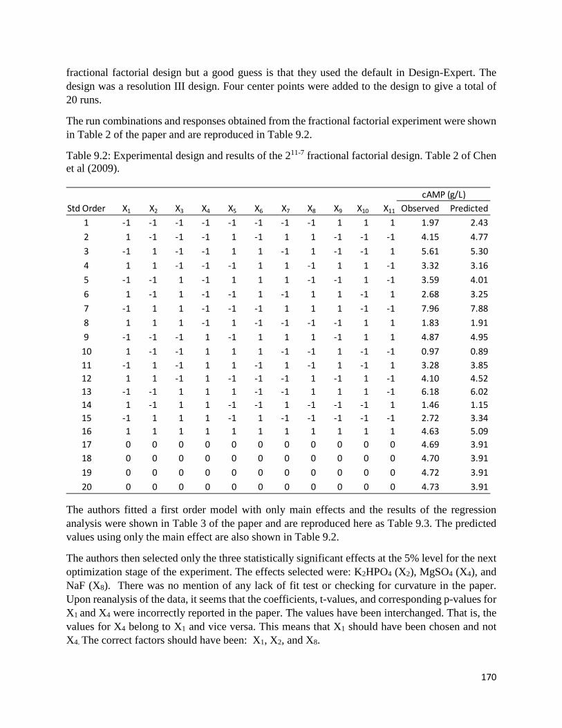
170
fractional factorial design but a good guess is that they used the default in Design-Expert. The design was a resolution III design. Four center points were added to the design to give a total of 20 runs.
The run combinations and responses obtained from the fractional factorial experiment were shown in Table 2 of the paper and are reproduced in Table 9.2.
Table 9.2: Experimental design and results of the 211-7 fractional factorial design. Table 2 of Chen et al (2009).
The authors fitted a first order model with only main effects and the results of the regression analysis were shown in Table 3 of the paper and are reproduced here as Table 9.3. The predicted values using only the main effect are also shown in Table 9.2.
The authors then selected only the three statistically significant effects at the 5% level for the next optimization stage of the experiment. The effects selected were: K2HPO4 (X2), MgSO4 (X4), and NaF (X8). There was no mention of any lack of fit test or checking for curvature in the paper. Upon reanalysis of the data, it seems that the coefficients, t-values, and corresponding p-values for X1 and X4 were incorrectly reported in the paper. The values have been interchanged. That is, the values for X4 belong to X1 and vice versa. This means that X1 should have been chosen and not X4. The correct factors should have been: X1, X2, and X8.
Std Order X1 X2 X3 X4 X5 X6 X7 X8 X9 X10 X11 Observed Predicted1 -1 -1 -1 -1 -1 -1 -1 -1 1 1 1 1.97 2.432 1 -1 -1 -1 1 -1 1 1 -1 -1 -1 4.15 4.773 -1 1 -1 -1 1 1 -1 1 -1 -1 1 5.61 5.304 1 1 -1 -1 -1 1 1 -1 1 1 -1 3.32 3.165 -1 -1 1 -1 1 1 1 -1 -1 1 -1 3.59 4.016 1 -1 1 -1 -1 1 -1 1 1 -1 1 2.68 3.257 -1 1 1 -1 -1 -1 1 1 1 -1 -1 7.96 7.888 1 1 1 -1 1 -1 -1 -1 -1 1 1 1.83 1.919 -1 -1 -1 1 -1 1 1 1 -1 1 1 4.87 4.9510 1 -1 -1 1 1 1 -1 -1 1 -1 -1 0.97 0.8911 -1 1 -1 1 1 -1 1 -1 1 -1 1 3.28 3.8512 1 1 -1 1 -1 -1 -1 1 -1 1 -1 4.10 4.5213 -1 -1 1 1 1 -1 -1 1 1 1 -1 6.18 6.0214 1 -1 1 1 -1 -1 1 -1 -1 -1 1 1.46 1.1515 -1 1 1 1 -1 1 -1 -1 -1 -1 -1 2.72 3.3416 1 1 1 1 1 1 1 1 1 1 1 4.63 5.0917 0 0 0 0 0 0 0 0 0 0 0 4.69 3.9118 0 0 0 0 0 0 0 0 0 0 0 4.70 3.9119 0 0 0 0 0 0 0 0 0 0 0 4.72 3.9120 0 0 0 0 0 0 0 0 0 0 0 4.73 3.91
cAMP (g/L)

171
Table 9.3: Regression results of the fractional factorial design. Table 3 of Chen et al (2009). Factor Coefficient t-Value P-value Intercept 3.9080 22.0111 0.000000* X1 -0.1812 -0.9130 0.387887 X2 0.4737 2.3866 0.044088* X3 0.1737 0.8753 0.406921 X4 -0.8150 -4.1057 0.003411* X5 0.0725 0.3652 0.724405 X6 -0.1587 -0.7997 0.446958 X7 0.4500 2.2669 0.053141 X8 1.3150 6.6245 0.000165* X9 0.1662 0.8375 0.426612 X10 0.1037 0.5226 0.615371 X11 -0.4162 -2.0969 0.069266
R2 = 0.9084. * Statistically significant at 95% confidence level
For the optimization stage of the experiment, the authors performed a path of steepest ascent to determine the proper levels for the central composite design. This was given in Table 4 of the paper. The final levels used for the three chosen factors from the fractional factorial design were shown in Table 5 of the paper and are reproduced here in Table 9.4.
Table 9.4: Levels of the factors tested in the central composite design (modified from Table 5 of Chen et al, 2009).
Factor Levels of factors -1.68 -1 0 1 1.68 K2HPO4 (A, g/L) 9.64 11 13 15 16.36 MgSO4 (B, g/L) 0.64 2 4 6 7.36 NaF (C, g/L) 0.032 0.1 0.2 0.3 0.368*
In Table 5 of the paper, the axial point of factor C was incorrectly listed as 0.268.
The central composite design with two center points has 16 runs. The design and the experimental results were shown in Table 6 of the paper and are reproduced here in Table 9.5. A full second-order model was then fitted to the data resulting in the following prediction equation:
𝑌𝑌 = 8.44 − 0.15 𝐴𝐴 − 0.29 𝐵𝐵 − 0.17 𝐶𝐶 − 0.60 𝐴𝐴2 − 0.58 𝐵𝐵2 − 0.48 𝐶𝐶2 − 0.26 𝐴𝐴𝐵𝐵 + 0.20 𝐴𝐴𝐶𝐶+ 0.035 𝐵𝐵𝐶𝐶
The equation gave a R2 of 0.9556. The regression results were given in Table 8 of the paper and are given here as Table 9.6. The predicted values are also shown in Table 9.5.
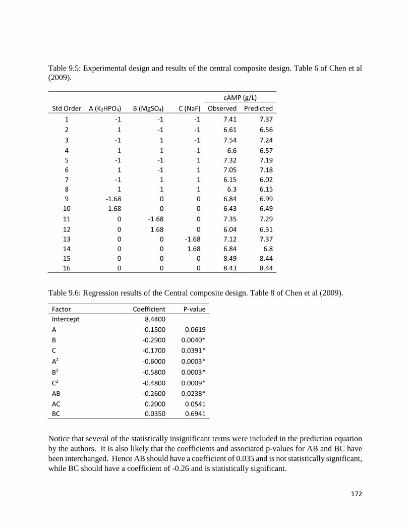
172
Table 9.5: Experimental design and results of the central composite design. Table 6 of Chen et al (2009).
cAMP (g/L) Std Order A (K2HPO4) B (MgSO4) C (NaF) Observed Predicted
1 -1 -1 -1 7.41 7.37 2 1 -1 -1 6.61 6.56 3 -1 1 -1 7.54 7.24 4 1 1 -1 6.6 6.57 5 -1 -1 1 7.32 7.19 6 1 -1 1 7.05 7.18 7 -1 1 1 6.15 6.02 8 1 1 1 6.3 6.15 9 -1.68 0 0 6.84 6.99
10 1.68 0 0 6.43 6.49 11 0 -1.68 0 7.35 7.29 12 0 1.68 0 6.04 6.31 13 0 0 -1.68 7.12 7.37 14 0 0 1.68 6.84 6.8 15 0 0 0 8.49 8.44 16 0 0 0 8.43 8.44
Table 9.6: Regression results of the Central composite design. Table 8 of Chen et al (2009).
Factor Coefficient P-value Intercept 8.4400 A -0.1500 0.0619 B -0.2900 0.0040* C -0.1700 0.0391* A2 -0.6000 0.0003* B2 -0.5800 0.0003* C2 -0.4800 0.0009* AB -0.2600 0.0238* AC 0.2000 0.0541 BC 0.0350 0.6941
Notice that several of the statistically insignificant terms were included in the prediction equation by the authors. It is also likely that the coefficients and associated p-values for AB and BC have been interchanged. Hence AB should have a coefficient of 0.035 and is not statistically significant, while BC should have a coefficient of -0.26 and is statistically significant.
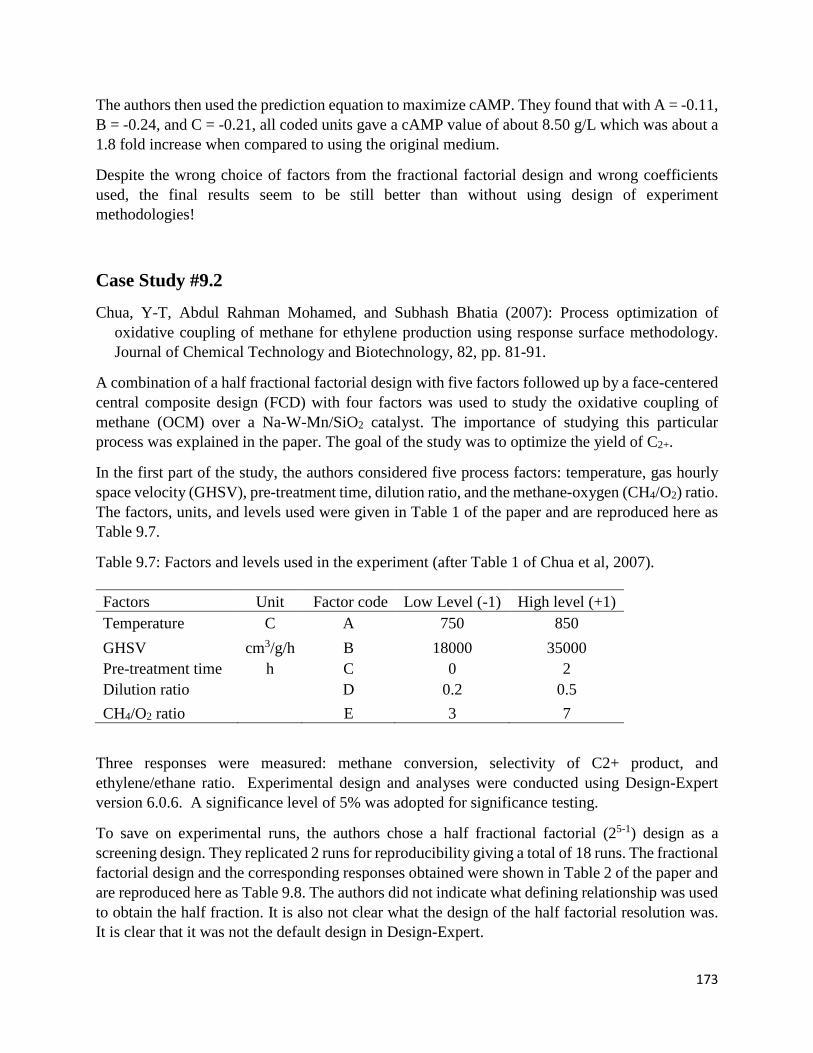
173
The authors then used the prediction equation to maximize cAMP. They found that with A = -0.11, B = -0.24, and C = -0.21, all coded units gave a cAMP value of about 8.50 g/L which was about a 1.8 fold increase when compared to using the original medium.
Despite the wrong choice of factors from the fractional factorial design and wrong coefficients used, the final results seem to be still better than without using design of experiment methodologies!
Case Study #9.2
Chua, Y-T, Abdul Rahman Mohamed, and Subhash Bhatia (2007): Process optimization of oxidative coupling of methane for ethylene production using response surface methodology. Journal of Chemical Technology and Biotechnology, 82, pp. 81-91.
A combination of a half fractional factorial design with five factors followed up by a face-centered central composite design (FCD) with four factors was used to study the oxidative coupling of methane (OCM) over a Na-W-Mn/SiO2 catalyst. The importance of studying this particular process was explained in the paper. The goal of the study was to optimize the yield of C2+.
In the first part of the study, the authors considered five process factors: temperature, gas hourly space velocity (GHSV), pre-treatment time, dilution ratio, and the methane-oxygen (CH4/O2) ratio. The factors, units, and levels used were given in Table 1 of the paper and are reproduced here as Table 9.7.
Table 9.7: Factors and levels used in the experiment (after Table 1 of Chua et al, 2007). Factors Unit Factor code Low Level (-1) High level (+1) Temperature C A 750 850 GHSV cm3/g/h B 18000 35000 Pre-treatment time h C 0 2 Dilution ratio D 0.2 0.5 CH4/O2 ratio E 3 7
Three responses were measured: methane conversion, selectivity of C2+ product, and ethylene/ethane ratio. Experimental design and analyses were conducted using Design-Expert version 6.0.6. A significance level of 5% was adopted for significance testing.
To save on experimental runs, the authors chose a half fractional factorial (25-1) design as a screening design. They replicated 2 runs for reproducibility giving a total of 18 runs. The fractional factorial design and the corresponding responses obtained were shown in Table 2 of the paper and are reproduced here as Table 9.8. The authors did not indicate what defining relationship was used to obtain the half fraction. It is also not clear what the design of the half factorial resolution was. It is clear that it was not the default design in Design-Expert.

174
Table 9.8: Experimental matrix of 2(5-1) fractional factorial design. Table 2 of Chua et al (2007).
The last two runs were considered repeat tests for reproducibility checking. They were not used in the ANOVA or regression models. For methane conversion, the authors fitted a linear model shown in Equation 4 of the paper, given by (in coded factors): CH4 conversion (%) = 35.24 + 1.24 A – 3.44 B + 2.69 C – 3.42 D + 2.30 E + 5.16 AB – 0.96 AC + 1.69 AD + 0.23 AE – 4.23 BC + 2.53 BE – 2.89 ABE + 7.06 ACD The authors stated that the selected effects in the equation were all statistically insignificant although AB, BC, and ACD have greater effects over the model. It is not clear why the authors included three-factor interaction terms in the model. These effects are usually ignored in practice. It is likely that the selected model is flawed. For the selectivity of C2+ product, the ANOVA results are shown in Table 3 of the paper and are reproduced here in Table 9.9. The authors then suggested the following equation to represent C2+ selectivity (Equation 5 of the paper): C2+ selectivity (%) = 28.11 + 0.056 A + 5.74 B + 3.52 C – 4.61 D + 13.91 E – 3.69 AB + 9.04 AD
- 4.40 AE + 12.41 BC – 16.33 BD + 5.48 BE + 4.83 ABE The ANOVA results show that only factor A (temperature) was not statistically significant at the 5% level.
Run A B C D E CH4 Conversion (%) C2+ Selectivity (%) C2H4/C2H6 ratio1 850 35000 2 0.5 7 40.43 62.09 1.642 850 35000 0 0.2 7 54.45 52.72 2.073 750 35000 2 0.5 7 19.96 34.38 0.44
4 750 18000 0 0.2 3 35.96 13.90 1.285 850 18000 0 0.2 3 31.93 8.31 1.206 750 35000 2 0.2 3 30.98 57.18 1.097 750 18000 0 0.5 7 34.77 55.11 0.868 850 18000 2 0.5 3 45.94 30.76 3.259 850 18000 0 0.5 7 23.34 47.68 1.7610 750 35000 0 0.2 3 15.08 25.05 1.4711 750 18000 2 0.5 3 41.83 2.79 1.7612 850 35000 2 0.2 3 29.66 45.48 2.3713 850 18000 2 0.5 7 47.46 29.70 2.1214 750 18000 2 0.5 7 33.48 37.55 0.7115 850 35000 0 0.2 3 45.86 13.87 1.2016 750 35000 0 0.2 7 31.68 63.75 0.7917 750 35000 0 0.2 7 32.61 65.75 0.7918 750 35000 0 0.2 7 31.63 66.28 0.80
ResponsesFactors

175
Table 9.9: ANOVA table of C2+ selectivity. Table 3 of Chua et al (2007).
The authors examined the two-factor interaction plots and concluded that interactions between factors AB, AE, and BE were not statistically significant in this study and hence the temperature factor was dropped from the next phase of experimentation. For the C2H4/C2H6 ratio, the authors did not provide any ANOVA results or model. However, some explanation regarding this response was given in the paper. From the initial fractional factorial results, the authors concluded that the ANOVA was dominated by the C2+ selectivity response and that the temperature variable could be fixed at 850 °C for the next round of experimentation. For the optimization study, the authors chose a four factor face-centered central composite design (FCD) with six center points. The levels were the same ones used in the fractional factorial design. The FCD required 16 runs for the factorial points, 8 runs for the axial points, and 6 center-points. Hence a total of 30 experiments were conducted. An additional response, called the C2+ yield (%) was added. (This can be calculated from methane conversion and C2+ selectivity; details are given in the paper.) The FCD and responses obtained are shown in Table 4 of the paper and are reproduced here in Table 9.10. The key goal was to maximize the C2+ yield hence the focus was on analysing this response. The authors did not show the ANOVA tables for any of the responses analysed. Only the prediction equation in coded factors for C2+ yield was given. This is Equation 6 of the paper, given by: C2+ yield (%) = 20.63 + 2.34 A + 2.28 B – 0.53 C + 4.30 D – 1.75 AB + 0.87 AC – 0.30 AD
- 5.19 BC – 0.70 BD – 2.09 CD.
Sum of MeanSource Squares d.f. square F-value Prob> F
Model 5805.62 12 483.80 418.79 0.0002
A 0.05 1 0.05 0.04 0.8476B 263.70 1 263.70 228.26 0.0006C 99.40 1 99.40 86.05 0.0027D 84.92 1 84.92 73.50 0.0033E 1547.07 1 1547.07 1339.16 <0.0001AB 145.04 1 145.04 125.55 0.0015AD 653.41 1 653.41 565.60 0.0002AE 206.51 1 206.51 178.75 0.0009BC 1232.06 1 1232.06 1066.49 <0.0001BD 1066.35 1 1066.35 923.05 <0.0001BE 240.35 1 240.35 208.05 0.0007ABE 372.68 1 372.68 322.60 0.0004Residual 3.47 3 1.16Corr. Total 5809.08 15

176
No goodness of fit statistics were given and there was no indication of whether all the terms were statistically significant. Table 9.10: Experimental matrix of 24 full factorial with central composite design. Table 4 of Chua et al (2007).
The authors then compared the results obtained by the DOE method with those obtained using an incipient wetness impregnation, and mixture slurry methods. They found that the results were almost identical.
GHSV Pretreat Dilution CH4/O2 CH4 C2+ C2+ C2H4/C2H6
Run (cm3/g/h) time (h) ratio ratio Conv (%) select (%) yield (%) ratio1 18000 0 0.2 3 32.78 9.02 2.96 1.202 35000 0 0.2 3 46.54 14.97 6.97 1.25
3 18000 2 0.2 3 44.63 51.44 22.96 2.724 35000 2 0.2 3 43.99 47.09 20.71 2.375 18000 0 0.5 3 43.62 25.85 11.28 2.766 35000 0 0.5 3 46.78 65.71 30.74 2.077 18000 2 0.5 3 36.12 32.72 11.82 3.258 35000 2 0.5 3 49.37 30.80 15.21 2.139 18000 0 0.2 7 25.61 57.13 14.63 1.15
10 35000 0 0.2 7 54.45 52.72 28.71 2.0711 18000 2 0.2 7 42.01 77.12 32.40 1.5312 35000 2 0.2 7 43.18 73.75 31.85 1.3213 18000 0 0.5 7 42.49 62.15 26.41 1.7614 35000 0 0.5 7 35.40 70.73 25.04 1.1515 18000 2 0.5 7 48.11 31.61 15.21 2.1216 35000 2 0.5 7 38.54 59.29 22.85 1.6417 18000 1 0.35 5 37.42 65.42 24.48 1.9318 35000 1 0.35 5 37.96 58.66 22.27 1.4819 26500 0 0.35 5 20.74 60.58 12.56 1.2020 26500 2 0.35 5 41.83 65.50 27.40 1.3021 26500 1 0.2 5 41.78 61.76 25.80 1.4922 26500 1 0.5 5 30.66 61.72 18.92 1.3923 26500 1 0.35 3 46.84 51.10 23.94 1.6324 26500 1 0.35 7 36.66 73.56 26.97 1.2025 26500 1 0.35 5 25.60 67.98 17.40 1.9926 26500 1 0.35 5 27.94 71.82 20.07 1.6827 26500 1 0.35 5 33.10 56.92 18.84 1.8528 26500 1 0.35 5 27.01 69.27 18.71 1.4229 26500 1 0.35 5 25.61 67.42 17.27 1.7530 26500 1 0.35 5 23.91 64.94 15.53 1.63
Factors Responses
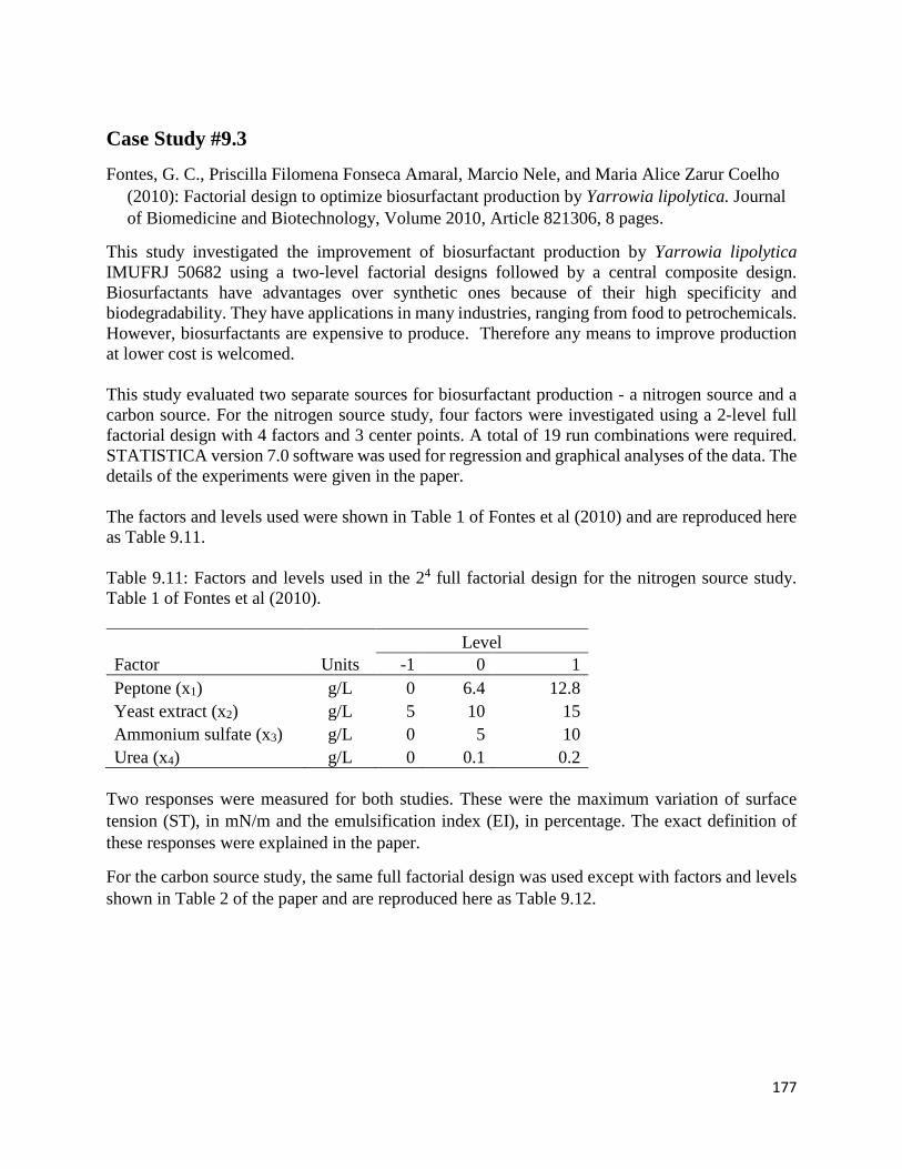
177
Case Study #9.3
Fontes, G. C., Priscilla Filomena Fonseca Amaral, Marcio Nele, and Maria Alice Zarur Coelho (2010): Factorial design to optimize biosurfactant production by Yarrowia lipolytica. Journal of Biomedicine and Biotechnology, Volume 2010, Article 821306, 8 pages.
This study investigated the improvement of biosurfactant production by Yarrowia lipolytica IMUFRJ 50682 using a two-level factorial designs followed by a central composite design. Biosurfactants have advantages over synthetic ones because of their high specificity and biodegradability. They have applications in many industries, ranging from food to petrochemicals. However, biosurfactants are expensive to produce. Therefore any means to improve production at lower cost is welcomed. This study evaluated two separate sources for biosurfactant production - a nitrogen source and a carbon source. For the nitrogen source study, four factors were investigated using a 2-level full factorial design with 4 factors and 3 center points. A total of 19 run combinations were required. STATISTICA version 7.0 software was used for regression and graphical analyses of the data. The details of the experiments were given in the paper. The factors and levels used were shown in Table 1 of Fontes et al (2010) and are reproduced here as Table 9.11. Table 9.11: Factors and levels used in the 24 full factorial design for the nitrogen source study. Table 1 of Fontes et al (2010). Level Factor Units -1 0 1 Peptone (x1) g/L 0 6.4 12.8 Yeast extract (x2) g/L 5 10 15 Ammonium sulfate (x3) g/L 0 5 10 Urea (x4) g/L 0 0.1 0.2
Two responses were measured for both studies. These were the maximum variation of surface tension (ST), in mN/m and the emulsification index (EI), in percentage. The exact definition of these responses were explained in the paper.
For the carbon source study, the same full factorial design was used except with factors and levels shown in Table 2 of the paper and are reproduced here as Table 9.12.

178
Table 9.12: Factors and levels used in the 24 full factorial design for the carbon source study (Table 2 of Fontes et al, 2010). Level Factor Units -1 0 1 Glycerol (z1) % w/v 0 1 2 Olive oil (z2) % w/v 0 2 4 Hexadecane (z3) %w /v 0 1 2 Glucose (z4) % w/v 0 2 4
The run combinations and results for the nitrogen source experiment were given in Table 3 of the paper and reproduced here as Table 9.13. Table 9.13: Experimental design and results of the 24 full factorial design for nitrogen source evaluation (Table 3 of Fontes et al, 2010)
Std Order x1 x2 x3 x4 ST EI 1 -1 -1 -1 -1 6.5 37.3 2 1 -1 -1 -1 14.5 26.1 3 -1 1 -1 -1 5.1 27 4 1 1 -1 -1 4 1 5 -1 -1 1 -1 16.6 45.3 6 1 -1 1 -1 22 52.2 7 -1 1 1 -1 19.5 40.6 8 1 1 1 -1 13 50 9 -1 -1 -1 1 7.5 35.7
10 1 -1 -1 1 6 30.6 11 -1 1 -1 1 9.3 13 12 1 1 -1 1 4.6 6.2 13 -1 -1 1 1 15.2 40.3 14 1 -1 1 1 16.3 50.1 15 -1 1 1 1 21.1 60.4 16 1 1 1 1 9.4 43.2 17 0 0 0 0 13 26 18 0 0 0 0 11.4 24 19 0 0 0 0 11 25.4
For the nitrogen source study, the authors used a Pareto chart to display the ranked order of the effects and which effects were statistically significant. For the emulsification index (EI), the order of significant effects was x3, x2x3, x2, x1x3, x1x2, and x1. Other effects were not statistically significant at the 5% level. The regression equation is thus:
EI = 33.4 – 2.5 x1 – 4.7 x2 + 12.8 x3 – 2.5 x1x2 + 3.6 x1x3 + 5.5 x2x3

179
For the variation in surface tension (ST), the order of the significant effects were x3, x1x2, x1x4, and x2. Other effects were not statistically significant. The regression equation is given by:
ST = 11.9 – 1.16 x2 + 4.7 x3 – 2.3 x1x2 – 1.4 x1x4.
These equations are collectively known as Equation 1 in the paper.
Notice the equation for ST is not hierarchical as x4 is missing. The R2 values for EI and ST were reported as 0.87 and 0.86, respectively.
Table 9.14: Experimental design and results of the 24 full factorial design for carbon source evaluation. Table 3 of Fontes et al (2010).
Std Order z1 z2 z3 z4 ST EI
1 -1 -1 -1 -1 9 6.9 2 1 -1 -1 -1 19.5 62.3 3 -1 1 -1 -1 2 11.6 4 1 1 -1 -1 11 25.5 5 -1 -1 1 -1 2.6 12.8 6 1 -1 1 -1 10.7 70.2 7 -1 1 1 -1 2 27.5 8 1 1 1 -1 9.9 39.3 9 -1 -1 -1 1 27.8 56.2
10 1 -1 -1 1 20.2 82.9 11 -1 1 -1 1 14.4 48.8 12 1 1 -1 1 14.8 40 13 -1 -1 1 1 14.9 47.3 14 1 -1 1 1 12.6 76.8 15 -1 1 1 1 14.4 38.9 16 1 1 1 1 13 26 17 0 0 0 0 10.9 42.3 18 0 0 0 0 9.8 43.1 19 0 0 0 0 11.2 43.9
For the carbon source study, Pareto charts showed that for EI, the ordered significant effects were z1, z1z2, z4, z2, z1z4, z3z4, and z2z3. Others were not statistically significant at the 5% level. For ST, the ordered significant effects were z4, z1z4, z3, z2, z2z3, and z1. Other effects were not statistically significant at the 5% level. According to the authors, although z2 (Olive oil) and z3 (Hexadecane) were statistically significant, they present a negative effect. Hence z1 (glycerol) and x4 (glucose) were considered the best substrates to increase biosurfactant production. The authors then performed another set of experiments using only z1 and z4 but in a rotatable CCD design with an additional response - the carbon to nitrogen (C/N) ratio. The factors and levels used in the CCD was shown in Table 5 of the paper and are reproduced here as Table 9.15.

180
Table 9.15: Coded and actual levels of the two variables in the CCD. Table 5 of Fontes et al, 2010).
Level Factor Units -1.41 -1 0 1 1.41 Glycerol (z1) % w/v 0.59 1 2 3 3.41 Glucose (z4) % w/v 1.17 2 4 6 6.83
The CCD had eight runs plus three center points giving a total of 11 combinations. The design and results of the three responses are shown in Table 6 of the paper and are reproduced here as Table 9.16.
Table 9.16: Experimental design and results of the CCD. Table 6 of Fontes et al (2010).
Std Order z1 z4 C/N EI ST
1 -1 -1 5.9 51.4 11.8 2 1 -1 10.4 66.2 13.6 3 -1 1 13.3 60.8 12.9 4 1 1 17.8 67.3 16 5 -1.41 0 8.7 54.1 12.1 6 1.41 0 15.1 57.8 15 7 0 -1.41 6.6 61.4 12.4 8 0 1.41 17.1 73.7 16.2 9 0 0 11.9 81.8 19.5
10 0 0 11.9 81.1 19 11 0 0 11.9 80.9 20.1
The authors fitted a second-order regression to the responses and obtained the following equations for EI and ST. This set of equations is Equation 2 in the paper, shown below:
𝐸𝐸𝐸𝐸 = 81.3 + 4.8 𝑧𝑧1 − 6.9 𝑧𝑧12 + 1.9 𝑧𝑧4 − 12.7 𝑧𝑧42 − 2.0 𝑧𝑧1𝑧𝑧4
𝑆𝑆𝑆𝑆 = 19.5 + 1.2 𝑧𝑧1 − 2.6 𝑧𝑧12 + 0.9 𝑧𝑧4 − 3.0 𝑧𝑧42 No ANOVA results were given but the R2 for both equations were given as 0.99.
The above mathematical models were validated by using mean values at the central points. The authors stated that the experimental EI and ST values perfectly agreed with the predicted maximum.
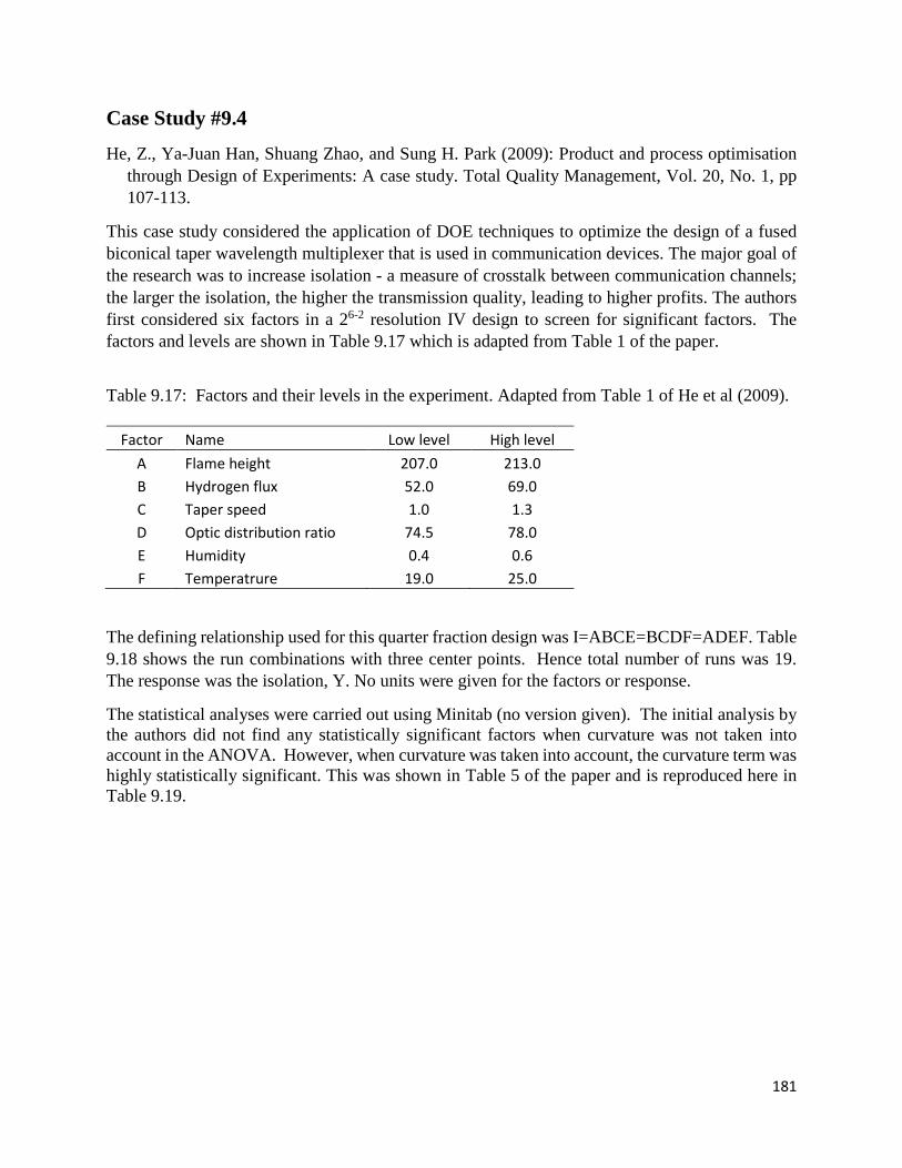
181
Case Study #9.4
He, Z., Ya-Juan Han, Shuang Zhao, and Sung H. Park (2009): Product and process optimisation through Design of Experiments: A case study. Total Quality Management, Vol. 20, No. 1, pp 107-113.
This case study considered the application of DOE techniques to optimize the design of a fused biconical taper wavelength multiplexer that is used in communication devices. The major goal of the research was to increase isolation - a measure of crosstalk between communication channels; the larger the isolation, the higher the transmission quality, leading to higher profits. The authors first considered six factors in a 26-2 resolution IV design to screen for significant factors. The factors and levels are shown in Table 9.17 which is adapted from Table 1 of the paper.
Table 9.17: Factors and their levels in the experiment. Adapted from Table 1 of He et al (2009).
Factor Name Low level High level A Flame height 207.0 213.0 B Hydrogen flux 52.0 69.0 C Taper speed 1.0 1.3 D Optic distribution ratio 74.5 78.0 E Humidity 0.4 0.6 F Temperatrure 19.0 25.0
The defining relationship used for this quarter fraction design was I=ABCE=BCDF=ADEF. Table 9.18 shows the run combinations with three center points. Hence total number of runs was 19. The response was the isolation, Y. No units were given for the factors or response.
The statistical analyses were carried out using Minitab (no version given). The initial analysis by the authors did not find any statistically significant factors when curvature was not taken into account in the ANOVA. However, when curvature was taken into account, the curvature term was highly statistically significant. This was shown in Table 5 of the paper and is reproduced here in Table 9.19.

182
Table 9:18: Experimental arrangement for the 26-2IV (coded variables). Table 2 of He et al (2009)
Std order Run order A B C D E F Y
1 10 -1 -1 -1 -1 -1 -1 21.4 2 3 1 -1 -1 -1 1 -1 19.4 3 14 -1 1 -1 -1 1 1 22.2 4 2 1 1 -1 -1 -1 1 22.3 5 6 -1 -1 1 -1 1 1 24.5 6 7 1 -1 1 -1 -1 1 20.1 7 9 -1 1 1 -1 -1 -1 19.5 8 4 1 1 1 -1 1 -1 20.8 9 16 -1 -1 -1 1 -1 1 20.6
10 17 1 -1 -1 1 1 1 18.9 11 13 -1 1 -1 1 1 -1 23.4 12 18 1 1 -1 1 -1 -1 23.6 13 8 -1 -1 1 1 1 -1 22.6 14 5 1 -1 1 1 -1 -1 18.7 15 15 -1 1 1 1 -1 1 23.5 16 12 1 1 1 1 1 1 23.7 17 19 0 0 0 0 0 0 26.5 18 11 0 0 0 0 0 0 24.8 19 1 0 0 0 0 0 0 27.2
Table 9.19: Estimated effects and coefficients for Y (coded units). Table 5 of He et al (2009).
Term Effect Coeff SE Coeff T P Constant 21.575 0.2275 94.85 0.000* A -1.2750 -0.6375 0.2275 -2.8 0.049* B 1.6000 0.8000 0.2275 3.52 0.025* Constant 0.2000 0.1000 0.2275 0.44 0.683 D 0.6000 0.3000 0.2275 1.32 0.258 E 0.7250 0.3625 0.2275 1.59 0.186 F 0.8000 0.4000 0.2275 1.76 0.153 A*B 1.7250 0.8625 0.2275 3.79 0.019* A*C -0.4250 -0.2125 0.2275 -0.93 0.403 A*D -0.0250 -0.0125 0.2275 -0.05 0.959 A*E -1.2000 -0.6000 0.2275 -2.64 0.058 A*F -1.7500 -0.8750 0.2275 -0.38 0.720 B*D 1.7500 0.8750 0.2275 3.85 0.018* B*F 0.3000 0.1500 0.2275 0.66 0..546 Ct. Pt. 4.5917 0.5725 8.02 0.001* S=0.909899, R-sq = 97.01%, R-sq (adj) = 86.54%
Note: *means that the P-value is less than 0.05, and the corresponding term is significant.
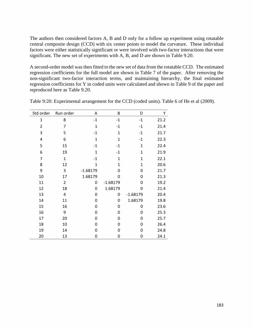
183
The authors then considered factors A, B and D only for a follow up experiment using rotatable central composite design (CCD) with six center points to model the curvature. These individual factors were either statistically significant or were involved with two-factor interactions that were significant. The new set of experiments with A, B, and D are shown in Table 9.20. A second-order model was then fitted to the new set of data from the rotatable CCD. The estimated regression coefficients for the full model are shown in Table 7 of the paper. After removing the non-significant two-factor interaction terms, and maintaining hierarchy, the final estimated regression coefficients for Y in coded units were calculated and shown in Table 9 of the paper and reproduced here as Table 9.20. Table 9:20: Experimental arrangement for the CCD (coded units). Table 6 of He et al (2009).
Std order Run order A B D Y 1 8 -1 -1 -1 21.2 2 7 1 -1 -1 21.4 3 5 -1 1 -1 21.7 4 6 1 1 -1 22.3 5 15 -1 -1 1 22.4 6 19 1 -1 1 21.9 7 1 -1 1 1 22.1 8 12 1 1 1 20.6 9 3 -1.68179 0 0 21.7
10 17 1.68179 0 0 21.3 11 2 0 -1.68179 0 19.2 12 18 0 1.68179 0 21.4 13 4 0 0 -1.68179 20.4 14 11 0 0 1.68179 19.8 15 16 0 0 0 23.6 16 9 0 0 0 25.3 17 20 0 0 0 25.7 18 10 0 0 0 26.4 19 14 0 0 0 24.8 20 13 0 0 0 24.1

184
Table 9.21: Final estimated regression coefficients for Y (coded units). Table 9 of He et al (2009).
Term Coeff SE Coeff T P Constant 24.9404 0.4396 56.737 0.000* A -0.1371 0.2916 -0.470 0.646 B 0.2563 0.2916 0.879 0.396 D -0.0446 0.2916 -0.153 0.881 A*A -0.9508 0.2839 -3.349 0.005* B*B -1.3750 0.2839 -4.843 0.000* D*D -1.4457 0.2839 -5.092 0.000* S=1.078, R-sq = 80.0%, R-sq (adj) = 70.8%
Note: *means that the P-value is less than 0.05, and the corresponding term is significant.
The final prediction equation in coded units is (Equation 1 of the paper):
𝑦𝑦� = 24.9404 − 0.1371 𝑥𝑥1 + 0.2563 𝑥𝑥2 − 0.0446 𝑥𝑥3 − 0.9508 𝑥𝑥12 − 1.375 𝑥𝑥22 − 1.4457𝑥𝑥32
where: x1 is the flame height, x2 is the hydrogen flux, and x3 is the optic distribution ratio. The optimum conditions were near the center points with x1 = -0.072, x2 = 0.093 and x3 = -0.015. The overall optimum condition for all factors were A = 210, B = 61, C = 1.00, D = 76, E = 0.4, and F = 19.
According to the authors, the isolation was 20 before optimization and 24.9404 after optimization with a 95% confidence interval of (23.9907, 25.8900), which was confirmed by confirmation runs.
Case Study #9.5
Raj, R. E., and B.S.S. Daniel (2011): Customization of closed-cell aluminum foam properties using design of experiments. Material Science and Engineering A, 528, pp. 2067-2075.
This study investigated factors that would influence the properties of closed-cell aluminum foam using experiments based on a fractional factorial design followed by a face-centered central composite design. According to the authors, aluminum foams are useful for various applications due to their high energy absorbing capacity, light weight, and high specific stiffness. The characteristic properties of interest are relative density, average pore diameter, and the average cell aspect ratio. The process of foaming and measurement of properties were described in the paper.
In the first stage of the experiment, the authors considered four major influencing factors - holding time, amount of TiH2, amount of calcium, and the stirring time after calcium addition. A half fraction of a two-level factorial design (24-1) with the four factors was used. The factors and levels are summarized in Table 9.22.

185
Table 9.22: Factors and levels used in the fractional factorial design
Factor Name Units Low level (-1) High level (+1) A Holding time s 80 120 B Amount of TiH2 wt % 0.6 1.0 C Amount of Ca wt % 0.8 1.2 D Stirring time for Ca min 8 12
Design-Expert 7.1.3 was used for the experimental design and subsequent statistical analysis and modeling. The defining relationship for the 24-1 design was not mentioned in the paper. It is assumed that the default in Design-Expert was used.
Three responses were measured - relative density, the average pore diameter (mm), and the cell aspect ratio.
The experimental design and results are shown in Table 1 of the paper and are shown here in Table 9.23.
Table 9.23: Phase I experimental design conditions and their corresponding structural properties of the closed-cell aluminum foam. Table 1 of Raj et al, 2011).
The ANOVA results for the three responses were summarized by the authors in Table 2 of the paper and are reproduced here as Table 9.24.
Table 9.24: ANOVA summary and the model statistic result of the phase-I half fractional factorial design of experiments. Table 2 of Raj et al (2011).
The 24-1 design is a resolution IV design, hence only the main effects can be cleanly estimated. The two-factor interactions are aliased with other two-factor interactions. The authors used Pareto
Exp No. Holding time
(A)Amount of TiH2
(B)Amount of Ca
(C)Stirring time
(D)Relative density
Average pore diameter (mm)
Cell aspect ratio
1 80 0.6 0.8 8 0.267 2.883 1.0192 120 0.6 0.8 12 0.266 3.120 1.364
3 80 1.0 0.8 12 0.176 3.063 1.0424 120 1.0 0.8 8 0.196 3.137 1.0725 80 0.6 1.2 12 0.225 3.020 1.0546 120 0.6 1.2 8 0.305 2.923 1.0407 80 1.0 1.2 8 0.157 3.274 1.0618 120 1.0 1.2 12 0.179 3.300 1.200
Process parameters Structural properties
Response Model type F-vlaue p-value Adj R-squared Pred R-squared Signal-to Noise ratioRelative density Factorial (R2FI) 36.43 0.0269 0.9620 0.8262 15.356Average pore diameter Factorial (R2FI) 119.25 0.0083 0.9883 0.9465 34.883Cell aspect ratio Factorial (R2FI) 11.38 0.0827 0.8811 0.4566 9.644

186
charts to display the effects and determined that only factor A (holding time) and factor B (amount of TiH2) were considered as significant factors for further investigation. The exact form of the reduced two-factor interaction models in Table 9.24 was not mentioned.
For the second phase of the investigation, the authors chose a face-centered central composite design with five center points. The range for factor A was changed to 60 - 140 (instead of 80 - 100), and for factor B it was changed to 0.5 - 1.5 (instead of 0.6 - 1.0). The face-centered CCD had 8 factorial points and 5 center points. The new design and experimental results were shown in Table 3 of the paper and are reproduced here in Table 9.25.
The ANOVA results were summarized by the authors in Table 4 of the paper and are reproduced here in Table 9.26.
Table 9.25: Phase II experimental design conditions and their corresponding structural properties of the closed-cell aluminum foam. Table 3 of Raj et al (2011).
Table 9.26: ANOVA summary and the model statistic result of the phase-II CCD. Table 4 of Raj et al v(2011).
From Table 9.26, a quadratic model fitted the relative density response well while the linear model fitted the other two responses. However, it was not mentioned in the paper which terms in the
Exp No. Holding time
(A)Amount of TiH2
(B) Relative densityAverage pore
diameter (mm) Cell aspect ratio
1 60 0.5 0.351 2.186 1.0082 100 0.5 0.337 2.240 1.091
3 140 0.5 0.286 3.325 1.1804 60 1.0 0.159 2.559 1.0105 100 1.0 0.148 3.200 1.0876 140 1.0 0.123 3.407 1.1207 60 1.5 0.102 3.204 1.1018 100 1.5 0.095 3.644 1.0259 140 1.5 0.080 4.486 1.25910 100 1.0 0.107 3.139 1.06311 100 1.0 0.108 2.931 1.08512 100 1.0 0.116 3.232 1.10713 100 1.0 0.100 3.251 1.084
Process parameters Structural properties
Response Model type F-vlaue p-value Adj R-squared Pred R-squared Signal-to Noise ratioRelative density Quadratic 62.49 0.0001 0.9624 0.9168 21.664Average pore diameter Linear 52.07 0.0001 0.8949 0.8185 24.505Cell aspect ratio Linear 7.78 0.0092 0.5306 0.1194 8.093

187
model were statistically significant and which were not. The authors presented the regression models for each of the responses. These were Equations 2, 3, and 4 in the paper. They are reproduced below:
Relative density = 0.8343 – 0.0019846 A – 0.9453 B + 0.00053 AB + 0.0000047166 A2
+ 0.3302 B2
Average pore diameter (mm) = 0.5785 + 0.0136 A + 1.1944 B
Cell aspect ratio = 1.0217 + 0.0014307 A – 0.2810 B – 0.00017375 AB + 0.0000028632 A2
+ 0.1829 B2
It is not clear why the regression equation for the cell aspect ratio was a quadratic instead of a linear model as shown in Table 9.26. No validation was done for any of the models.
Case Study #9.6
Vicente, G., Mercedes Martinez, and Jose Aracil (2007): Optimization of integrated biodiesel production. Part I. A study of the biodiesel purity and yield. Bioresource Technology, 98, pp. 1724-1733.
This study investigated the development and optimization of potassium hydroxide catalyzed synthesis of fatty acid methyl esters (biodiesel) from sunflower oil. The authors first started the experiments with a full factorial design with three factors and four center points. Then the design was augmented by adding star or axial points to model non-linearity observed in the responses. The factors and levels investigated were temperature, initial catalyst concentration, and methanol:vegetable oil molar ratio. The factors and levels used in the factorial experiment are summarized in Table 9.27.
Table 9.27: Factors and levels used in the biodiesel experiment.
The responses were the biodiesel purity (P in % weight) and the biodiesel yield (Y in % weight). The experimental design and results were given in Table 1 of the paper and are reproduced here in Table 9.28.
Factor (coded) Name Unit Low level (-1) Mid level (0) High Level (+1)T (XT) Temperature °C 25 45 65C (XC) Initial catalyst concentration % wt 0.5 1.0 1.5MR (XMR) Vegetable oil molar ratio 4.5 6.0 7.5

188
9.28: Experiment matrix and results: factorial and centre points. Table 1 of Vicente et al (2007).
The software to carry out the statistical analyses was not mentioned in the paper. The statistical tests were performed at a 5% significance level. The statistical model obtained for P (purity), in terms of coded units was:
P = 92.6137 + 3.0337 XT + 6.1462 XC + 2.7562 XMR – 2.7487 XTXC + 0.3221 XTXMR
-1.5662 XCXMR (r2 = 0.994)
And for the yield Y was:
Y = 95.8950 – 1.6775 XT – 2.4200 XC + 0.0800 XMR – 1.8725 XTXC – 0.4275 XTXMR
-0.4050 XCXMR (r2 = 0.995)
These were Equations 1 and 2 in the paper. Equations in terms of actual factors were also given in the paper.
For response P, the authors identified the effects T, C, MR, T.C, T.MR and C.MR as statistically significant. Curvature was also statistically significant. For response Y, statistically significant effects were T, C, T.C, and T.MR. The curvature was also statistically significant.
To model the nonlinear effect, the authors augmented the two-level factorial design by adding star or axial points at (+α and –α) to the design making it a rotatable central composite design with 18 runs. The α used was 1.68. It was not mentioned whether these new runs were put in a separate block. The additional star points were shown in Table 3 of the paper and are reproduced here as Table 9.29.
Run T (°C) C (% wt) MR XT XC XMR P (%wt) Y (% wt)1 65 1.5 7.5 1 1 1 99.95 89.422 65 1.5 4.5 1 1 -1 98.14 90.433 25 0.5 7.5 -1 -1 1 84.08 99.284 25 1.5 4.5 1 1 -1 97.00 97.175 65 0.5 7.5 -1 -1 1 97.50 98.326 25 1.5 7.5 -1 1 1 99.95 96.887 65 0.5 4.5 1 -1 -1 87.00 98.708 25 0.5 4.5 -1 -1 -1 77.29 96.969 45 1 6 0 0 0 99.80 98.4010 45 1 6 0 0 0 99.72 97.9411 45 1 6 0 0 0 99.38 98.6312 45 1 6 0 0 0 99.44 97.48

189
9.29: Experimental matrix and results: star points. Table 3 of Vicente et al (2007).
The authors then fitted a full second-order model to the responses and obtained the following equations (in coded units) for P and for Y (Equations 5 and 6 in the paper):
𝑃𝑃 = 99.4978 + 2.7266 𝑋𝑋𝑇𝑇 + 6.9623 𝑋𝑋𝐶𝐶 + 3.5861 𝑋𝑋𝑀𝑀𝐶𝐶 − 0.8896 𝑋𝑋𝑇𝑇2 − 2.7487 𝑋𝑋𝑇𝑇𝑋𝑋𝐶𝐶 + 0.3212 𝑋𝑋𝑇𝑇𝑋𝑋𝑀𝑀𝑀𝑀 − 4.3598 𝑋𝑋𝐶𝐶2 − 1.5662 𝑋𝑋𝐶𝐶𝑋𝑋𝑀𝑀𝑀𝑀 − 2.3534 𝑋𝑋𝑀𝑀𝑀𝑀2 (r2 = 0.969)
𝑌𝑌 = 98.1063 − 1.4510 𝑋𝑋𝑇𝑇 − 2.0058 𝑋𝑋𝐶𝐶 + 0.2985 𝑋𝑋𝑀𝑀𝐶𝐶 − 0.7808 𝑋𝑋𝑇𝑇2 − 2.0225 𝑋𝑋𝑇𝑇𝑋𝑋𝐶𝐶 − 0.5775 𝑋𝑋𝑇𝑇𝑋𝑋𝑀𝑀𝑀𝑀 − 1.0036 𝑋𝑋𝐶𝐶2 − 0.2550 𝑋𝑋𝐶𝐶𝑋𝑋𝑀𝑀𝑀𝑀 − 0.3283 𝑋𝑋𝑀𝑀𝑀𝑀2 (r2 = 0.964)
Equations in terms of actual factors were also given in the paper. However there is no indication which of the regression coefficients were statistically significant.
Optimization of purity and yield are assumed to have used the quadratic equations developed. The optimal values of the variables were temperature at 25 °C, a 1.3% wt catalyst concentration, and a 6:1 methanol:sunflower oil molar ratio. Using these values the predicted purity was 100% wt and yield was 98.4 %wt.
Case Study #9.7
Zhou, J., Yong-Hong Wang, Ju Chu, Ling-Zhi Luo, Ying-Ping Zhuang, and Si-Liang Zhang (2009): Optimization of cellulose mixture for efficient hydrolysis of steam-exploded corn stover by statistically designed experiments. Bioresource Technology, 100, pp. 819-825.
In this study, statistically designed experiments were used to optimize the composition of cellulose mixture to maximize the amount of glucose produced from a steam-exploded corn stover - the purpose being to improve enzymatic hydrolytic efficiency and reduce production cost. A half fraction six-factor fractional factorial (26-1) design with 32 runs and four center points was first used as a screening experiment. This was followed up with a rotatable central composite design with only four factors identified from the screening experiment. The six factors and their levels used in the screening experiment were shown in Table 2 of the paper and are reproduced here with slight modifications as Table 9.30. The choice of factors and experimental methods used were described in the paper. Design-Expert Version 6.0.4 software was used for the design and analysis of the experiments.
Run T (°C) C (% wt) MR XT XC XMR P (%wt) Y (% wt)13 78.63 1 6 +α 0 0 99.82 94.2814 11.36 1 6 -α 0 0 92.11 97.3715 45 1.84 6 0 +α 0 99.80 92.4516 45 0.16 6 0 -α 0 72.50 97.9417 45 1 8.52 0 0 +α 99.83 97.7718 45 1 3.47 0 0 -α 96.44 83.82

190
Table 9.30: Factors and code values of fractional factorial design. Table 2 of Zhou et al (2009).
The screening experiment was a resolution VI design meaning all main effects are aliased with five factor interactions and all two-factor interactions are aliased with four-factor interactions. This allows a full two-factor interaction model to be fitted without bias. The default defining relationship in Design-Expert was used to generate the 26-1 fractional factorial design. The design and experimental results were shown in Table 1 of the paper and are reproduced here as Table 9.31. The response measured was the glucose production in mg/ml.
The authors fitted a two-factor interaction model to the experimental data and produced the following regression equation (Equation 3 in the paper). All terms were used in the model regardless of their significance.
Glucose (mg/ml) = 4.875 + 0.665 x1 + 0.643 x2 + 0.291 x3 + 0.427 x4 + 0.427 x5 + 0.313 x6 + 0.119 x1x2 + 0.153 x1x3 – 0.0056 x1x4 – 0.051 x1x4 + 0.063 x2x5 – 0.074 x2x6 + 0.142 x3x4 + 0.51 x3x5 + 0.256 x3x6 – 0.085 x4x5 + 0.074 x4x6 – 0.016 x5x6
The predicted values using the above equation were also given in Table 9.31. The estimated coefficients and their corresponding F and p-values were given in Table 3 in the paper and are reproduced here in Table 9.32. The full ANOVA results were not reported. From Table 9.32, many of the effects were not statistically significant at the 5% level. No other goodness-of-fit statistics other than the R2 value were given. A closer look at the coefficients showed that some if not all the coefficients might have been incorrectly estimated or that the data used was not the same as reported in Table 9.31. The estimated intercept term in the regression model was given as 4.875. This value should be equal to the average value of the responses which is 5.025 with the center points included in the analysis, and 4.92 without including the center points. Furthermore, upon reanalysis of the data, the R2 value is much lower than reported and the predicted R2 is in fact negative for the two-factor interaction model. The predicted results at the center points (when all factors are at the 0 value) in Table 9.31 were all 5.85. Using the prediction equation, the predicted values should all be 4.875. The authors also indicated that there was statistically significant curvature and hence a follow up experiment to model the nonlinearity was required. This part of the ANOVA results was not shown in the paper.
Factors Code-1 0 +1
Cel7A x1 1 3 5Cel6A x2 2 6 10Cel6B x3 0.5 1.0 1.5Cel7B x4 0.5 2.5 4.5Cel12A x5 1.5 2.25 3Cel61A x6 0.3 0.5 0.7
Levels of factors (µmol/l)

191
Table 9.31: Experimental design and results of 26-1 fractional factorial design. Table 1 of Zhou et al (2009).
Runs x1 x2 x3 x4 x5 x6 Experiment Predicted1 -1 1 -1 -1 1 -1 5.39 5.202 -1 1 1 -1 1 1 5.13 4.953 1 1 1 1 -1 -1 6.03 6.114 -1 -1 1 1 1 1 5.74 5.325 -1 -1 1 1 -1 -1 3.29 3.266 -1 -1 -1 1 -1 1 3.69 3.367 1 -1 -1 1 -1 -1 3.75 3.798 -1 -1 1 -1 -1 1 2.83 3.269 1 -1 -1 1 1 1 4.85 5.00
10 -1 1 -1 -1 -1 1 3.92 3.4211 -1 1 1 -1 -1 -1 3.62 3.2012 1 1 -1 1 -1 1 6.42 6.3413 1 1 1 -1 -1 1 5.68 6.0714 -1 -1 -1 -1 1 1 3.82 3.5415 1 1 -1 -1 -1 -1 4.64 4.9516 1 1 1 -1 1 -1 5.70 5.9317 -1 1 -1 1 1 1 4.31 5.3218 1 -1 1 1 1 -1 4.73 5.1319 1 1 -1 1 1 -1 8.87 8.5020 -1 1 -1 1 -1 -1 4.83 4.8321 -1 -1 -1 -1 -1 -1 2.66 2.9722 1 1 -1 -1 1 1 6.24 6.1623 -1 1 1 1 -1 1 5.50 5.3224 -1 1 1 1 1 -1 5.46 5.6325 -1 -1 -1 1 1 -1 4.48 3.9526 1 -1 -1 -1 1 -1 3.96 4.1527 -1 -1 1 -1 1 -1 3.74 3.6728 1 1 1 1 1 1 6.82 6.6329 1 -1 1 -1 1 1 6.04 6.0930 1 -1 -1 -1 -1 1 4.18 4.0231 1 -1 1 1 -1 1 6.49 6.4532 1 -1 1 -1 -1 -1 4.63 3.6133 0 0 0 0 0 0 6.09 5.8534 0 0 0 0 0 0 5.64 5.8535 0 0 0 0 0 0 5.80 5.8536 0 0 0 0 0 0 5.94 5.85
x1 = Cel7A, x2 = Cel6A, x3 = Cel6B, x4 = Cel7B, x5 = Cel12A, and x6 = Cel61A.
Glucose production (mg/ml)Experimental factors and code levels

192
Table 9.32: Regression analysis of the 26-1 fractional factorial design. Table 3 of Zhou et al (2009).
Since the full ANOVA results were not given, it is not possible to check whether the authors used the wrong data in their analysis or the data reported in Table 9.31 was wrong.
Based on the results of Table 9.32, the authors identified only factors x1, x2, x4 and x5 and their interactions as significant. They then used a four-factor rotatable central composite design (CCD) with six center points in order to develop a second-order model for optimization of glucose production. The total number of runs required was 30 - 16 for the factorial points, eight for the axial points, and six center points. The axial points were at α = ±2.0 for a rotatable design. The CCD and results were given in Table 4 in the paper and are reproduced here as Table 9.33. The other two factors, x3 and x6, were kept at their central values.
Factors Coefficient estimate F-value p-valueIntercept# 4.875 15.870 0.0044**Cel7A (x1) 0.666 73.080 0.0007**Cel6A (x2) 0.643 96.860 0.0002**Cel6B (x3) 0.291 0.163 0.3110Cel7B (x4) 0.427 13.590 0.0042**Cel12A (x5) 0.427 1.780 0.026*Cel61A (x6) 0.313 2.310 0.0222*x1x2 0.119 6.070 0.0097**x1x3 0.153 0.186 0.2139x1x4 -0.0056 14.940 0.0036**x1x5 -0.051 0.920 0.047*x1x6 0.222 0.470 0.0842x2x3 -0.097 0.142 0.4228x2x4 0.108 8.430 0.0068**x2x5 0.063 1.290 0.039*x2x6 -0.074 0.131 0.5371x3x4 0.142 0.166 0.2472x3x5 0.051 0.124 0.6676x3x6 0.256 0.880 0.0514x4x5 -0.085 1.630 0.027*x4x6 0.074 0.131 0.5371x5x6 -0.016 0.073 0.8857(p-value, * <0.05, ** <0.01, and R2 = 0.9532)# Table 3 of Zhou et al (2009) reported this incorrectly as "Model"

193
Table 9.33: Design and results of central composite design. Table 4 of Zhou et al (2009).
The authors fitted a full second-order regression model to the experimental results and obtained the following equation (Equation 4 in the paper):
𝐺𝐺𝐺𝐺𝐺𝐺𝐺𝐺𝐺𝐺𝐺𝐺𝐺𝐺 (𝑚𝑚𝑚𝑚 𝑝𝑝𝐺𝐺𝑝𝑝 𝑚𝑚𝐺𝐺)= 7.141 + 0.361 𝑥𝑥1 + 0.347 𝑥𝑥2 + 0.005 𝑥𝑥4 + 0.052 𝑥𝑥5 − 0.344 𝑥𝑥12 − 0.112 𝑥𝑥22
− 0.216 𝑥𝑥42 − 0.553 𝑥𝑥52 + 0.545 𝑥𝑥1𝑥𝑥2 − 0.064 𝑥𝑥1𝑥𝑥4 − 0.047 𝑥𝑥1𝑥𝑥5 + 0.064 𝑥𝑥2𝑥𝑥4− 0.062 𝑥𝑥2𝑥𝑥5 + 0.005 𝑥𝑥4𝑥𝑥5
Run x1 x2 x4 x5 Experiment Predicted1 -1 -1 -1 -1 5.00 5.122 1 -1 -1 -1 4.64 4.503 -1 1 -1 -1 5.26 5.194 1 1 -1 -1 6.83 7.235 -1 -1 1 -1 5.39 5.596 1 -1 1 -1 5.51 5.197 -1 1 1 -1 5.39 5.458 1 1 1 -1 7.31 7.129 -1 -1 -1 1 5.44 5.9010 1 -1 -1 1 5.69 5.5711 -1 1 -1 1 5.00 5.2512 1 1 -1 1 7.12 7.1013 -1 -1 1 1 6.38 5.9214 1 -1 1 1 5.08 5.3315 -1 1 1 1 5.68 5.5316 1 1 1 1 7.50 7.2317 -2 0 0 0 5.19 5.0418 2 0 0 0 6.45 6.4919 0 -2 0 0 6.17 6.0020 0 2 0 0 7.33 7.3921 0 0 -2 0 6.88 6.2722 0 0 2 0 5.78 6.2823 0 0 0 -2 4.98 4.8324 0 0 0 2 4.99 5.0325 0 0 0 0 6.70 6.6726 0 0 0 0 6.75 6.6727 0 0 0 0 6.67 6.6728 0 0 0 0 6.59 6.6729 0 0 0 0 6.56 6.6730 0 0 0 0 6.75 6.67
Glucose production (mg/ml)Level of variabless

194
No ANOVA results were given and no indication of the goodness-of-fit was given. The predicted values based on the equation were also given in Table 9.33. Again it can be observed that at the center point values, the predicted values did not match those from the equation. The results in Table 9.33 showed values of 6.67, but they should have been 7.141 if the regression equation was used. So either the data were incorrectly reported or the fitted equations were incorrect.
The authors then used the regression equation to obtain the combination of the factors to give maximum glucose production. They found that the optimal concentrations of Cel7A (x1), Cel6A (x2), Cel7B (x4), and Cel 12A (x5) were 4.2, 8.1, 3.7, and 3.2 µmol/l, respectively.
The results were validated by the authors using additional verification experiments and they found that the glucose produced using the optimal combinations was 15.5 mg/ml - a 2.1 fold increase when compared to a control group without optimization.

195
______________________________________________ 10. REFERENCES
Chapter 1: General references
Anderson, M. and P. Whitcomb (2015): DOE Simplified: Practical tools for Effective Experimentation, 3rd Edition. CRC Press, Taylor and Francis Group, 252 pages.
Anderson, M. and P. Whitcomb (2016): RSM Simplified: Optimizing Processes Using Response Surface Methods for Design of Experiments, 2nd Edition. CRC Press, Taylor and Francis Group, 295 pages.
Anthony, Jiju (2003): Design of Experiments for Engineers and Scientists, Butterworth-Heinemann Press, 152 pages.
Berthouex, P. M. and Linfield C. Brown (2002): Statistics for Environmental Engineers, 2nd Edition. Lewis Publishers, 489 pages.
Box, G. E. P., J. Stuart Hunter, and W. G. Hunter (2005): Statistics for Experimenters, 2nd Edition, John Wiley and Sons, 639 pages.
Hicks, C. R. and Kenneth V. Turner, Jr. (1999): Fundamental Concepts in the Design of Experiments, 5th Edition, Oxford University Press, 565 pages.
Kuehl, Robert O. (2000): Design of Experiments: Statistical Principles of Research Design and Analysis, 2nd Edition. Duxbury Press, 666 pages.
Mason, R. L., R. F. Gunst, and J. L. Hess (2003): Statistical Design and Analysis of Experiments With Applications to Engineering and Science. John Wiley and Sons, 728 pages.
Montgomery, D. C. (2017): Design and Analysis of Experiments, 9th Edition, John Wiley and Sons, 752 pages.
Myers, R. H., D.C. Montgomery, and C.M. Anderson-Cook (2016): Response Surface Methodology: Process and Product Optimization Using Designed Experiments, 4th Edition, John Wiley and Sons, 856 Pages.
Ryan, Thomas P. (2007): Modern Experimental Design, Wiley-Interscience, 624 pages.
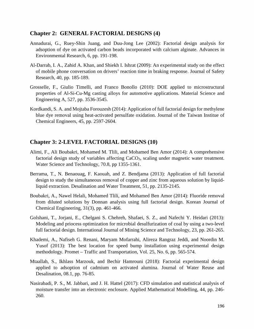
196
Chapter 2: GENERAL FACTORIAL DESIGNS (4)
Annadurai, G., Ruey-Shin Juang, and Duu-Jong Lee (2002): Factorial design analysis for adsoption of dye on activated carbon beads incorporated with calcium alginate. Advances in Environmental Research, 6, pp. 191-198.
Al-Darrab, I. A., Zahid A. Khan, and Shiekh I. Ishrat (2009): An experimental study on the effect of mobile phone conversation on drivers’ reaction time in braking response. Journal of Safety Research, 40, pp. 185-189.
Grosselle, F., Giulio Timelli, and Franco Bonollo (2010): DOE applied to microstructural properties of Al-Si-Cu-Mg casting alloys for automotive applications. Material Science and Engineering A, 527, pp. 3536-3545.
Kordkandi, S. A. and Mojtaba Forouzesh (2014): Application of full factorial design for methylene blue dye removal using heat-activated persulfate oxidation. Journal of the Taiwan Institue of Chemical Engineers, 45, pp. 2597-2604.
Chapter 3: 2-LEVEL FACTORIAL DESIGNS (10)
Alimi, F., Ali Boubakri, Mohamed M. Tlili, and Mohamed Ben Amor (2014): A comprehensive factorial design study of variables affecting CaCO3, scaling under magnetic water treatment. Water Science and Technology, 70.8, pp 1355-1361.
Berrama, T., N. Benaouag, F. Kaouah, and Z. Bendjama (2013): Application of full factorial design to study the simultaneous removal of copper and zinc from aqueous solution by liquid-liquid extraction. Desalination and Water Treatment, 51, pp. 2135-2145.
Boubakri, A., Nawel Helali, Mohamed Tlili, and Mohamed Ben Amor (2014): Fluoride removal from diluted solutions by Donnan analysis using full factorial design. Korean Journal of Chemical Engineering, 31(3), pp. 461-466.
Golshani, T., Jorjani, E., Chelgani S. Chehreh, Shafaei, S. Z., and Nafechi Y. Heidari (2013): Modeling and priocess optimization for microbial desulfurization of coal by using a two-level full factorial design. International Journal of Mining Science and Technology, 23, pp. 261-265.
Khademi, A., Nafiseh G. Renani, Maryam Mofarrahi, Alireza Rangraz Jeddi, and Noordin M. Yusof (2013): The best location for speed bump installation using experimental design methodology. Promet – Traffic and Transportation, Vol. 25, No. 6, pp. 565-574.
Mtaallah, S., Ikhlass Marzouk, and Bechir Hamrouni (2018): Factorial experimental design applied to adsoption of cadmium on activated alumina. Journal of Water Reuse and Desalination, 08.1, pp. 76-85.
Nasirabadi, P. S., M. Jabbari, and J. H. Hattel (2017): CFD simulation and statistical analysis of moisture transfer into an electronic enclosure. Applied Mathematical Modelling, 44, pp. 246-260.

197
Ridzuan, N., F. Adam, and Z. Yaacob (2016): Screening of factor influencing wax deposition using full factorial experimental design. Petroleum Science and Technology, Vol. 34, No. 1, pp. 84-90.
Shah, Mumtaj and S. K. Garg (2014): Application of 2k full factorial design in optimization of solvent-free microwave extraction of ginger essential oil. Journal of Engineering, Article ID 828606, 5 pages.
Yusoff, N. H. N., M. J. Ghazali, M. C. Isa, A. R. Daud, A. Muchtar, and S.M. Forghani (2012): Optimization of plasma spray parameters on the mechanical properties of agglomerated Al2O3-13%TiO2 coated mild steel. Materials and Design, 39, pp. 504-508.
Chapter 4: 2-LEVEL FRACTIONAL FACTORIAL DESIGNS (9)
Chen, J. P., S. L. Kim, and Y. P. Ting (2003): Optimization of membrane physical and chemical cleaning by a statistical designed approach. Journal of Membrane Science, 219, pp. 27-45.
Choi, Y.E., Y-S Yun, and J.M. Park (2002): Evaluation of factors promoting Astaxanthin production by a unicellular green alga, Haematococcus pluvialis, with fractional factorial design. Biotechnology Progress, 18, pp. 1170-1175.
Farris, S. and Luciano Piergiovanni (2008): Effects of ingredients and process conditions on ‘Amaretti’ cookies characteristics. International Journal of Food Science and Technology, 43, pp. 1395-1403.
Hajeeh, M. (2003): Estimating corrosion: a statistical approach. Materials and Design, 24, pp. 509-518.
Kazemi-Beydokhti, A., Hamed Azizi Namaghi, and Saeed Zeinali Heris (2013): Identification of the key variables on thermal conductivity of CuO nanofluid by a fractional factorial design approach. Numerical Heat Transfer, Part B, 64, pp. 480-495.
Levingstone, T. J., Malika Ardhaoui, Khaled Benyyounis, Lisa Looney, and Joseph T. Stokes (2015): Plasma sprayed hydroxyapatite coatings: Understanding process relationships using design of experiments analysis. Surface and Coatings Technology, 283, pp. 29-36.
Lucas, Y., Antonio Domingues, Driss Driochi, and Sylvie Treuillet (2006): Design of experiments for performance evaluation and parameter tuning of a road image processing chain. EURASIP Journal on Applied Signal Processing, Article ID 48012, pp. 1-10.
Ramakrishna, D. M., T. Viraraghavan (2006): Iron oxide coated sand for arsenic removal: investigation of coating parameters using factorial design approach. Practice Periodical of Hazardous, Toxic, and Radioactive Waste Management, Vol. 10, No. 4, pp. 198-206.
Samad, K. A., and Norazwina Zainol (2017): The use of factorial design for ferulic acid production by co-culture. Industrial Crops and Products, 95, pp. 202-206.

198
Chapter 5: 3-LEVEL FACTORIAL DESIGNS (6)
Ahmad, S., and Saeid A. Alghamdi (2014): A statistical approach to optimizing concrete mixture design. The Scientific World Journal, Vol. 2014, Article ID 561539, pp 1-7.
Alsobaai, Ahmed Mubarak (2013): Thermal cracking of petroleum residue oil using three level factorial design. Journal of King Saud University – Engineering Sciences, 25, pp. 21-28.
Amini, S., M. J. Nategh, and H. Soleimanimehr (2009): Application of design of experiments for modelling surface roughness in ultrasonic vibration turning. Proceedings Institution of Mechanical Engineers, Vol. 223, Part B: J. Engineering Manufacture, pp. 641-652.
Berrios, M., M.C. Gutierrez, M.A. Martin, and A. Martin (2009): Application of the factorial design of experiments to biodiesel production from lard. Fuel Processing Technology, 90, pp. 1447-1451.
Comoglu, B. A., Cansun Filik Iscen, and Semra IIhan (2015): The anaerobic treatment of pharmaceutical industry wastewater in an anaerobic batch and upflow packed-bed reactor. Desalination and Water Treatment, 2015, pp 1-12.
Martin-Lara, M. A., I. L. Rodriguez, G. Blazquez, and M. Calero (2011): Factorial experimental design for optimizing the removal conditions of lead ions from aqueous solutions by three wastes of olive-oil production. Desalination, 278, pp. 132-140.
Chapter 6: RSM: BOX-BEHNKEN DESIGNS (8)
Aslan, N. and Y. Cebeci (2007): Application of Box-Behnken design and response surface methodology for modeling of Turkish coals. Fuel, 86, pp. 90-97.
Cai, L, Haifu Wang, and Yawei Fu (2013): Freeze-thaw resistance of alkali-slag concrete based on response surface methodology. Construction and Building Materials, 49, pp. 70-76.
Jalali, M. R. and Mohammad Amin Sobati (2017): Intensification of oxidative desulfurization of gas oil by ultrasound irradiation: Optimization using Box-Behnken design (BBD). Applied Thermal Engineering, 111, pp. 1158-1170.
Kilickap, E. and Mesut Huseyinoglu (2010): Selection of optimum parameters on burr height using response surface methodology and genetic algorithm in drilling of AISI 304 stainless steel. Materials and Manufacturing Processes, 25, pp. 1068-1076.
Liu Junyan, Lin Li, Lizhen Zhou, Bing Li, and Zhenbo Xu (2017): Effect of ultrasound treatment conditions on Saccharomyces cerevisiae by response surface methodology. Microbial Pathogenesis, 111 pp. 497-502.
Muthukumar, M., D. Mohan, and M. Rajendran (2003): Optimization of mix proportions of mineral aggregates using Box-Behnken design of experiments. Cement and Concrete Composites, 25, pp. 751-758.

199
Sharifi, H., Seyed Majid Zabihzadeh, and Mohsen Ghorbani (2018): The application of response surface methodology on the synthesis of conductive polyaniline/cellulosic fiber nanocomposites. Carbohydrate Polymers, 194, pp. 384-394.
Zhang, H., Yanli Li, and Xiaogang Wu (2012): Statistical experiment design approach for the treatment of landfill leachate by photoelectro-fenton process. ASCE Journal of Environmental Engineering, Vol. 138, No. 3, pp. 278-285.
Chapter 7: RSM: CENTRAL COMPOSITE DESIGNS (Rotatable) (10)
Ahmad, A. L., S. Ismail, and S. Bhatia (2005): Optimization of coagulation-flocculation process for palm oil mill effluent using response surface methodology. Environmental Science and Technology, 39, pp. 2828-2834.
Bajpai, S., S. K. Gupta, Apurba Dey, M. K. Jha, Vidushi Bajpai, Saurabh Joshi, and Arvind Gupta (2012): Application of central composite design approach for removal of chromium (VI) from aqueous solution using weakly anionic resin: Modeling, optimization, and study of interactive variables. Journal of Hazardous Materials, 227-228, pp. 436-444.
Eren, I. and Figen Kaymak-Erktekin (2007): Optimization of osmotic dehydration of potato using response surface methodology. Journal of Food Engineering, 79, pp. 344-352.
Lakshminarayanan, A. K., V. E. Annamalai, and K. Elangovan (2015): Identification of optimum friction stir spot welding process parameters controlling the properties of low carbon automotive steel joints. Journal of Materials Research and Technology, 4 (3), pp. 262-272.
Mu, Y., Xian-Jun Zheng, and Han-Qing Yu (2009): Determining optimum conditions for hydrogen production from glucose by an anaerobic culture using response surface methodology (RSM). International Journal of Hydrogen Energy, 34, pp. 7959-7963.
Prasad, K. N., Fouad Abdulrahman Hassan, Bao Yang, Kin Weng Kong, Ramakrishnan Nagasundara Ramanan, Azrina Azlan, and Amin Ismail (2011): Response surface optimization for the extraction of phenolic compounds and antioxidant capacities of underutilised Mangifera pajang Kosterm peels. Food Chemistry, 1238, pp. 1121-1127.
Rastegar, S. O., S. M. Mousavi, S. A. Shojaosadati, and S. Sheibani (2011): Optimization of petroleum refinery effluent treatment in a UASB reactor using response surface methodology. Journal of Hazardous Materials, 197, pp. 26-32.
Singal, R., Prateek Seth, Dinesh Bangwal, and Savita Kaul (2012): Optimization of biodiesel production by response surface methodology and genetic algorithm. Journal of ASTM International, Vol. 9, NO. 5, pp. 1-7.

200
Wang, J.P., Yong-Zhen Chen, Xue-Wu Ge, and Han-Qing Yu (2007): Optimization of coagulation-flocculation process for a paper-recycling wastewater treatment using response surface methodology. Colloids and Surfaces A: Physicochemical Engineering Aspects, 302, pp. 204-210.
Yuen, X., Jia Liu, Guangming Zeng, Jingang Shi, Jingyi Tong, and Guohe Huang (2008): Optimization of conversion of waste rapeseed oil with high FFA to biodiesel using response surface methodology. Renewable Energy, 33, pp. 1678-1684.
Chapter 8: RSM: CENTRAL COMPOSITE DESIGNS (Face-Centered) (10)
Alvarez, M. J., N. Gil-Negrete, L. Ilzarbe, M. Tanco, E. Viles, and A. Asensio (2009): A computer experiment application to the design and optimization of a capacitive accelerometer. Applied Stochastic Models in Business and Industry, 25, pp. 151-162.
Chiang, Ko-Ta, and Fu-Ping Chang (2006): Application of response surface methodology in the parametric optimization of a pin-fin type heat sink. International Communications in Heat and Mass Transfer, 33, pp. 836-845.
Jenarthanan, M. P. and R. Jeyapaul (2014): Machinability study of carbon fibre reinforced polymer (CFRP) composites using design of experiment technique. Pigment & Resin Technology, 43/1, pp. 35-44.
Kwon, J-H, Sang-Moon Hwang, Chang-Min Lee, Kwang-Suk Kim, and Gun-Yong Hwang (2009): Application of response surface methodology (RSM) in microspeaker design used in mobile phones. IEEE Transactions on Magnetics, Vol. 45, N. 10, pp. 4550-4553.
Mohajeri, L., Hamidi Abdul Aziz, Mohamed Hasnain Isa, and Mohammad Ali Zahed (2010): A statistical experiment design approach for optimizing biodegradation of weathered crude oil in coastal sediments, Bioresource Technology, 1011, pp. 893-900.
Noordin, M. Y., V.C. Venkatesh, S. Sharif, S. Elting, and A. Abdullah (2004): Application of response surface methodology in describing the performance of coated carbide tools when turning AISI 1045 steel. Journal of Materials Processing Technology, 145, pp. 46-58.
Qian, Fuping and Mingyao Zhang (2005): Study of the natural vortex length of a cyclone with response surface methodology. Computers and Chemical Engineering, 29, pp. 2155-2162.
Sin, H. N., S. Yusof, N. Sheikh Abdul Hamid, and R. Abd. Rahman (2006): Optimization of enzymatic clarification of sapodilla juice using response surface methodology. Journal of Food Engineering, 73, pp. 313-319.
Tabaraki, Reza and Ashraf Nateghi (2011): Optimization of ultrasonic-assisted extraction of natural antioxidants from rice bran using response surface methodology. Ultrasonic Sonochemistry, 18, pp. 1279-1286.

201
Wee Shin Ling, Tye Ching Thian, and Subhash Bhatia (2010): Process optimization studies for the dehydration of alcohol-water system by inorganic membrane based pervaporation separation using design of experiments (DOE). Separation and Purification Technology, 71, pp. 192-199.
Chapter 9: COMBINATION DESIGNS (7)
Chen, X-C., Jian-Xin Bai, Jia-Ming Cao, Zhen-Jiang Li, Jian Xiong, Lei Zhang, Yuan Hong, and Han-Jie Ying (2009): Medium optimization for the production of cyclic adenosine 3’, 5’-monophosphate by Microbacterium sp. no. 205 using response surface methodology. Bioresource Technology, 100, pp. 919-924.
Chua, Y-T, Abdul Rahman Mohamed, and Subhash Bhatia (2007): Process optimization of oxidative coupling of methane for ethylene production using response surface methodology. Journal of Chemical Technology and Biotechnology, 82, pp. 81-91.
Fontes, G. C., Priscilla Filomena Fonseca Amaral, Marcio Nele, and Maria Alice Zarur Coelho (2010): Factorial design to optimize biosurfactant production by Yarrowia lipolytica. Journal of Biomedicine and Biotechnology, Volume 2010, Article 821306, 8 pages.
He, Z., Ya-Juan Han, Shuang Zhao, and Sung H. Park (2009): Product and process optimisation through Design of Experiments: A case study. Total Quality Management, Vol. 20, No. 1, pp 107-113.
Raj, R. E., and B.S.S. Daniel (2011): Customization of closed-cell aluminum foam properties using design of experiments. Material Science and Engineering A, 528, pp. 2067-2075.
Vicente, G., Mercedes Martinez, and Jose Aracil (2007): Optimization of integrated biodiesel production. Part I. A study of the biodiesel purity and yield. Bioresource Technology, 98, pp. 1724-1733.
Zhou, J., Yong-Hong Wang, Ju Chu, Ling-Zhi Luo, Ying-Ping Zhuang, and Si-Liang Zhang (2009): Optimization of cellulose mixture for efficient hydrolysis of steam-exploded corn stover by statistically designed experiments. Bioresource Technology, 100, pp. 819-825.

202
Appendix A: Summary of factors and responses for each case study.
CS #2.1, pages 8-9. Design: General factorial 3 Factors: Initial dye concentration, pH, Temperature 1 Response: Adsorption of Rhodomine 6G. CS #2.2, pages 10-12. Design: General factorial 3 Factors: Distance between cars, call duration, time of driving 1 Response: Driver’s reaction time. CS #2.3, pages 13-15. Design: General factorial 4 Factors: SDAS, Titanium content, copper content, T7 heat treatment 5 Responses: Equivalent diameter, roundness, yield strength, ultimate tensile strength, elongation to fracture. CS #2.4, pages 15-18. Design: General factorial 4 Factors: Reaction time, persulfate concentration, initial MB concentration, process temperature 1 Response: Color removal efficiency (%). CS #3.1, pages 19-22. Design: 2-level factorial 3 Factors: pH, flow rate, magnetic field 3 responses: Induction time, total precipitation rate, homogenous precipitation rate of CaCO3. CS #3.2, pages 22-25. Design: 2-level factorial 5 Factors: pH of initial solution, initial concentration of Zn or Cu, concentration of extractant, medium type of initial aqueous solution, stirring rate 2 responses: % removal of zinc (II), % removal of copper (II). CS #3.3, pages 26-28. Design: 2-level factorial 4 Factors: C, Q, A, T 2 responses: Fluoride removal efficiency, fluoride flux. CS #3.4, pages 29-31. Design: 2-level factorial 5 Factors: pH, particle size, Fe2+, pulp density, leaching time 1 response: sulfur reduction (%).
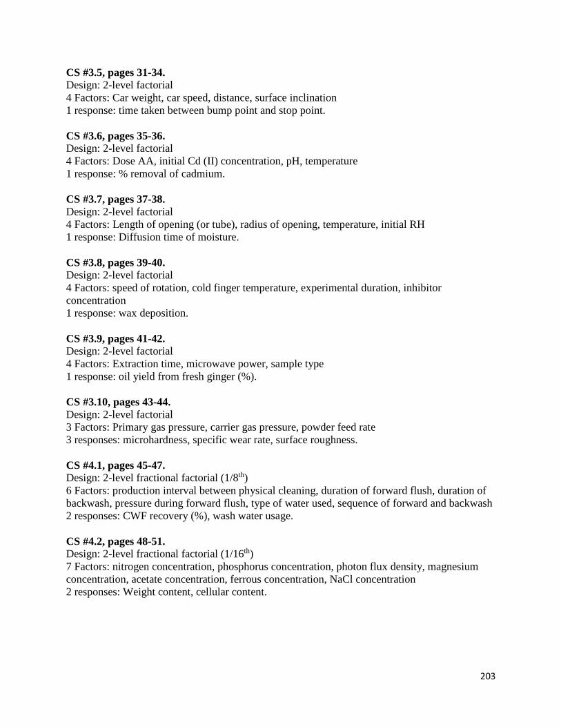
203
CS #3.5, pages 31-34. Design: 2-level factorial 4 Factors: Car weight, car speed, distance, surface inclination 1 response: time taken between bump point and stop point. CS #3.6, pages 35-36. Design: 2-level factorial 4 Factors: Dose AA, initial Cd (II) concentration, pH, temperature 1 response: % removal of cadmium. CS #3.7, pages 37-38. Design: 2-level factorial 4 Factors: Length of opening (or tube), radius of opening, temperature, initial RH 1 response: Diffusion time of moisture. CS #3.8, pages 39-40. Design: 2-level factorial 4 Factors: speed of rotation, cold finger temperature, experimental duration, inhibitor concentration 1 response: wax deposition. CS #3.9, pages 41-42. Design: 2-level factorial 4 Factors: Extraction time, microwave power, sample type 1 response: oil yield from fresh ginger (%). CS #3.10, pages 43-44. Design: 2-level factorial 3 Factors: Primary gas pressure, carrier gas pressure, powder feed rate 3 responses: microhardness, specific wear rate, surface roughness. CS #4.1, pages 45-47. Design: 2-level fractional factorial (1/8th) 6 Factors: production interval between physical cleaning, duration of forward flush, duration of backwash, pressure during forward flush, type of water used, sequence of forward and backwash 2 responses: CWF recovery (%), wash water usage. CS #4.2, pages 48-51. Design: 2-level fractional factorial (1/16th) 7 Factors: nitrogen concentration, phosphorus concentration, photon flux density, magnesium concentration, acetate concentration, ferrous concentration, NaCl concentration 2 responses: Weight content, cellular content.

204
CS #4.3, pages 52-55. Design: 2-level fractional factorial (1/2) 5 Factors: Fibre, F/S, egg white, temperature, time 4 responses: Hardness, moisture content, water activity, colour. CS #4.4, pages 55-59. Design: 2-level fractional factorial (1/2) 6 Factors: temperature, oxygen, urea, inhibitor, sulfide, chloride 1 response: corrosion rate. CS #4.5, pages 60-62. Design: 2-level fractional factorial (1/16th) 7 Factors: Temperature, particle volume fraction, APPS, pH of nanofluids, elapsed time, sonication time, density of nanoparticles 1 response: Ratio of thermal conductivity of nanofluids to base fluid (Knf/Kf). CS #4.6, pages 63-65. Design: 2-level fractional factorial (1/4) 5 Factors: Current, gas flow rate, powder feed rate, spray distance, carrier gas flow rate 3 responses: roughness, crystallinity, purity. CS #4.7, pages 65-67. Design: 2-level fractional factorial (1/16th) 8 Factors: Canny-Deriche filter, image amplification, edge low threshold, edge high threshold, contour closing, polygonal approximation, little chain threshold, slope threshold 1 response: covering rate CS #4.8, pages 67-70. Design: 2-level fractional factorial (1/16th) 7 Factors: pHc, T, Fe, N, Age, pHs, M 2 responses: percentage removal of As(V), percentage removal of As(III). CS #4.9, pages 70-72. Design: 2-level fractional factorial (1/8th) 7 Factors: temperature, pH agitation, water-to-substrate ratio, volume of inoculum, fermentation time, type of co-culture 1 response: Ferulic acid produced. CS #5.1, pages 73-75. Design: 3-level factorial 3 Factors: Cementitious materials content, water/cementitious materials ratio, fine/total aggregate ratio 2 responses: average compressive strength, standard deviation of compressive strength.

205
CS #5.2, pages 75-78. Design: 3-level factorial 3 Factors: Temperature, time, pressure 5 responses: conversion rate, yield of total distillate fuels, yield of the gasoline fraction, yield of the kerosene fraction, yield of the diesel fraction. CS #5.3, pages 78-81. Design: 3-level factorial 4 Factors: Vibration amplitude, depth of cut, feed rate, cutting speed 1 response: Surface roughness. CS #5.4, pages 82-83. Design: 3-level factorial 2 Factors: Agitation speed, catalyst concentration 1 response: FAME concentration. CS #5.5, pages 84-86. Design: 3-level factorial 3 Factors: Basal medium, wastewater, cosubstrate type 2 responses: average compressive strength, standard deviation of compressive strength. CS #5.6, pages 86-90. Design: 3-level factorial 3 Factors: Cementitious materials content, water/cementitious materials ratio, fine/total aggregate ratio 1 response: Percentage of COD removed. CS #6.1, pages 91-93. Design: RSM - BBD 3 Factors: Ball diameter, Grinding time, bond work index 3 responses: coarse, middle, and fine size fractions of coal. CS #6.2, pages 93-95. Design: RSM - BBD 3 Factors: A/S, slag, sand ratio 1 response: Frost resistance coefficient. CS #6.3, pages 96-97. Design: RSM - BBD 3 Factors: Oxidant to sulfur molar ratio, formic acid to oxidant ratio, sonication time 1 response: Sulfur removal (%).

206
CS #6.4, pages 98-99. Design: RSM - BBD 3 Factors: cutting speed, feed rate, point angle 1 response: Burr height. CS #6.5, pages 100-101. Design: RSM - BBD 3 Factors: Ultrasonic power, Irradiating time, pulse duty ratio 1 response: Ultrasound treatment efficiency. CS #6.6, pages 102-105. Design: RSM - BBD 6 Factors: Six grades of particle size (A to F) 1 response: Void content (%). CS #6.7, pages105-107. Design: RSM - BBD 3 Factors: Surfactant type, mass ratio of fibers/aniline, time of polymerization 1 response: Conductivity. CS #6.8, pages 107-110. Design: RSM - BBD 3 Factors: Ferrous iron dosage, hydrogen peroxide concentration, current density 2 responses: Percentage of color removal, COD removal. CS #7.1, pages 111-114. Design: RSM – rotatable CCD 3 Factors: Coagulant dosage, flocculant dosage, pH 2 responses: Turbidity, water recovery CS #7.2, pages 115-117 Design: RSM – rotatable CCD 4 Factors: Treatment time, pH, Cr(VI) concentration, adsorbent dose 1 response: Removal of Cr(VI) (%) CS #7.3, pages 118-120 Design: RSM – rotatable CCD 4 Factors: Temperature, sucrose concentration, salt, concentration, time. 4 responses: water loss, weight reduction, solid gain, water activity. CS #7.4, pages 120-123. Design: RSM – rotatable CCD 3 Factors: Rotational speed, plunge depth, dwell time 1 response: Tensile shear failure load.

207
CS #7.5, pages 123-125. Design: RSM – rotatable CCD 3 Factors: Rotational speed, plunge depth, dwell time 1 response: Tensile shear failure load. CS #7.6, pages 125-127. Design: RSM – rotatable CCD 3 Factors: Ethanol concentration, temperature, liquid/solid ratio 2 responses: Total phenolic content, antioxidant capacity. CS #7.7, pages 128-130. Design: RSM – rotatable CCD 3 Factors: hydraulic retention time, up flow velocity, influent COD 1 response: COD removal (%), biogas rate. CS #7.8, pages 131-132. Design: RSM – rotatable CCD 3 Factors: Temperature, catalyst concentration, molar ratio 1 response: Biodiesel yield. CS #7.9, pages 133-135. Design: RSM – rotatable CCD 3 Factors: Coagulant dosage, flocculant dosage, pH 1 response: Turbidity, sludge volume index (SVI). CS #7.10, pages 136-138. Design: RSM – rotatable CCD 4 Factors: Methanol/oil molar ratio, catalyst concentration, reaction time, temperature 1 response: Biodiesel conversion (%). CS #8.1, pages 139-142. Design: RSM – FCD 5 Factors: Thickness of seismic mass, thickness of beams, area seismic mass, length of beams, width of beams 1 response: Natural frequency. CS #8.2, pages 142-146. Design: RSM – FCD 4 Factors: Fin height, pin diameter, longitudinal pitch, transverse pitch 1 response: Thermal resistance, pressure drop. CS #8.3, pages 146-148. Design: RSM – FCD 3 Factors: Feed rate, cutting speed, depth of cut 1 response: Delamination factor.
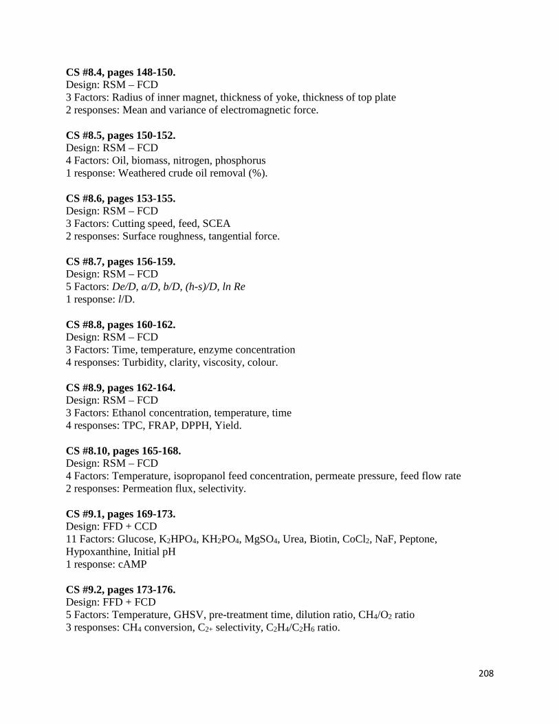
208
CS #8.4, pages 148-150. Design: RSM – FCD 3 Factors: Radius of inner magnet, thickness of yoke, thickness of top plate 2 responses: Mean and variance of electromagnetic force. CS #8.5, pages 150-152. Design: RSM – FCD 4 Factors: Oil, biomass, nitrogen, phosphorus 1 response: Weathered crude oil removal (%). CS #8.6, pages 153-155. Design: RSM – FCD 3 Factors: Cutting speed, feed, SCEA 2 responses: Surface roughness, tangential force. CS #8.7, pages 156-159. Design: RSM – FCD 5 Factors: De/D, a/D, b/D, (h-s)/D, ln Re 1 response: l/D. CS #8.8, pages 160-162. Design: RSM – FCD 3 Factors: Time, temperature, enzyme concentration 4 responses: Turbidity, clarity, viscosity, colour. CS #8.9, pages 162-164. Design: RSM – FCD 3 Factors: Ethanol concentration, temperature, time 4 responses: TPC, FRAP, DPPH, Yield. CS #8.10, pages 165-168. Design: RSM – FCD 4 Factors: Temperature, isopropanol feed concentration, permeate pressure, feed flow rate 2 responses: Permeation flux, selectivity. CS #9.1, pages 169-173. Design: FFD + CCD 11 Factors: Glucose, K2HPO4, KH2PO4, MgSO4, Urea, Biotin, CoCl2, NaF, Peptone, Hypoxanthine, Initial pH 1 response: cAMP CS #9.2, pages 173-176. Design: FFD + FCD 5 Factors: Temperature, GHSV, pre-treatment time, dilution ratio, CH4/O2 ratio 3 responses: CH4 conversion, C2+ selectivity, C2H4/C2H6 ratio.
209
CS #9.3, pages 177-180. Design: FD + CCD 4 Factors (Nitrogen source): Peptone, yeast extract, ammonium sulfate, urea 4 Factors (Carbon source): Glycerol, olive oil, hexadecane, glucose 2 responses: Surface tension, emulsification index (%). CS #9.4, pages 181-184. Design: FFD + FCD 6 Factors: Flame height, hydrogen flux, taper speed, optic distribution ratio, humidity, temperature 1 response: Isolation. CS #9.5, pages 184-187. Design: FFD + FCD 4 Factors: Holding time, amount of TiH2, amount of Ca, stirring time for Ca 3 responses: Relative density, average pore diameter, cell aspect ratio. CS #9.6, pages 187-189. Design: FD + CCD 3 Factors: Temperature, initial catalyst concentration, vegetable oil molar ratio 2 responses: Biodiesel purity, biodiesel yield. CS #9.7, pages 189-194. Design: FFD + CCD 6 Factors: Cel7A, Cel6A, Cel6B, Cel7B, Cel12A, Cel61A 1 response: Glucose production.
Dr. Leonard M. Lye, PEng, FCSCE, FEC, FCAE, FEIC Professor Emeritus, Faculty of Engineering and Applied Science Memorial University of Newfoundland, Canada.
Brief Biography
Dr. Leonard Lye is a happily retired professor in the Faculty of Engineering and Applied Science. Dr. Lye is the winner of numerous awards for teaching, community service, and service to the engineering profession. He is also an inventor and entrepreneur. He is the inventor of the DOE-GolferTM, and the DOE-SIM and DOE-SIM Pro IOS apps for teaching design of experiments principles which are used worldwide by corporations, universities, and six-sigma trainers.
About the book
This book provides a selection of 26 case studies that cover a wide range of DOE applications in engineering and science. Only papers where there is a complete set of data available for reanalysis were chosen. The selection is not exhaustive and does not cover every discipline of engineering or science. However, readers of the book should get a good sense of the wide application of DOE methods, and will try their hand at reanalyzing the published data. The methods most commonly used in the papers deal mainly with factorial designs, fractional factorial designs, and response surface methodologies, particularly the use of the central composite and Box-Behnken designs.
The book is ideal for students who have taken or is taking a course in DOE. It is also useful for those who want to learn more about the power of DOE methods or who are looking for research ideas. Each dataset is available in print form in the book and available as an Excel file (.xls) and as a Design-Expert® file (.dxpx). Hence this collection of case studies is also be a good resource for instructors of DOE.