Weather Modeling

Joseph Lutgen

May 15 2009

Abstract

This document is an essay of purely researched material. The essay focuseson weather modeling using differential equations. A basic understanding ofdifferential equations is suggested before reading the material herein.

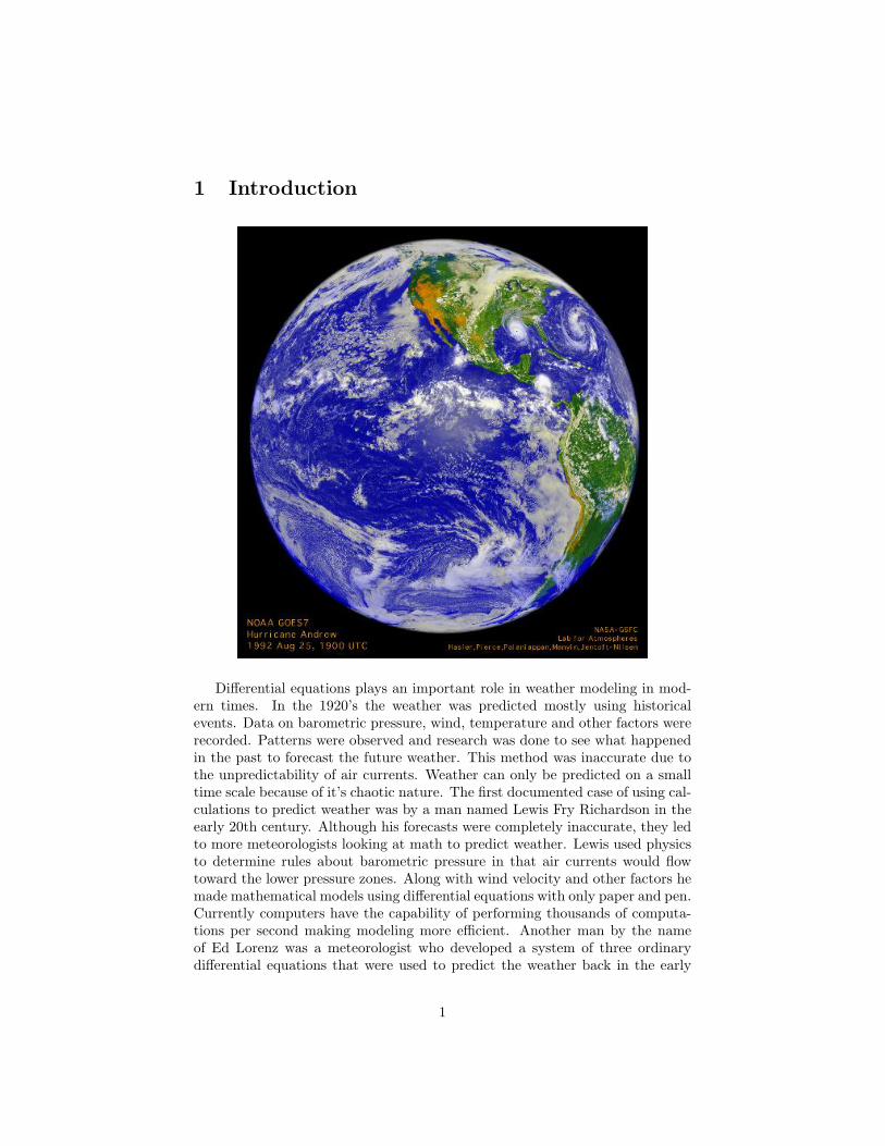
1 Introduction

Differential equations plays an important role in weather modeling in mod-ern times. In the 1920’s the weather was predicted mostly using historicalevents. Data on barometric pressure, wind, temperature and other factors wererecorded. Patterns were observed and research was done to see what happenedin the past to forecast the future weather. This method was inaccurate due tothe unpredictability of air currents. Weather can only be predicted on a smalltime scale because of it’s chaotic nature. The first documented case of using cal-culations to predict weather was by a man named Lewis Fry Richardson in theearly 20th century. Although his forecasts were completely inaccurate, they ledto more meteorologists looking at math to predict weather. Lewis used physicsto determine rules about barometric pressure in that air currents would flowtoward the lower pressure zones. Along with wind velocity and other factors hemade mathematical models using differential equations with only paper and pen.Currently computers have the capability of performing thousands of computa-tions per second making modeling more efficient. Another man by the nameof Ed Lorenz was a meteorologist who developed a system of three ordinarydifferential equations that were used to predict the weather back in the early

1

1960’s. Although these equations proved to be ineffective, they did show thesame pattern of unpredictability that occurs within the weather. Weather hasmany contributable factors. One such factor is the heat produced from the sunbeing varied over the surface of the earth. An additional factor is the differencesof air temperature over the surface of the earth. Vorticity also plays a majorpart in weather modeling. Due to the earth’s rotation, the geostrophic windpatterns are changed making twists and spirals which are high and low pressureareas. Another variability in weather is due to pressure in the atmosphere de-creasing as height increases. When air pressure decreases the temperature willdrop. Since precipitation is dependent on air pressure and air pressure is sochaotic, it is difficult to predict weather more than a week into the future.

2

2 Lorenz Ordinary Differential Equations

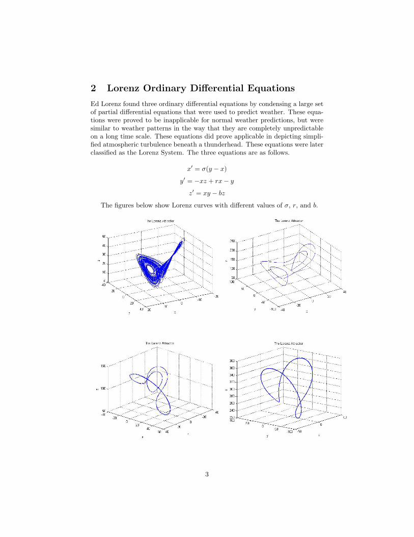
Ed Lorenz found three ordinary differential equations by condensing a large setof partial differential equations that were used to predict weather. These equa-tions were proved to be inapplicable for normal weather predictions, but weresimilar to weather patterns in the way that they are completely unpredictableon a long time scale. These equations did prove applicable in depicting simpli-fied atmospheric turbulence beneath a thunderhead. These equations were laterclassified as the Lorenz System. The three equations are as follows.

x′ = σ(y − x)

y′ = −xz + rx− y

z′ = xy − bz

The figures below show Lorenz curves with different values of σ, r, and b.

3

2.1 Finding Equilibrium in Lorenz attractors

To find the equilibrium solutions for the Lorenz attractor, the initial equationsare set to 0.

0 = σ(y − x)

0 = −xz + rx− y

0 = xy − bz

2.1.1 X-nullclines

To find the x-null cline, the equation below must be solved for y.

0 = σ(y − x)

Since σ is constant,

y = x

2.1.2 Y-nullclines

Since y = x, and 0 = −xz + rx− y, then

0 = −xz + rx− x

x(r − 1− z) = 0

So,x = 0 or z = r − 1

2.1.3 Z-nullclines

Now that y = x, and either x = 0 or z = r − 1

−bz + xy = 0

−bz + x2 = 0

So,

z = 0 or −r(r − 1) + x2 = 0→ x =√b(r − 1)

4

2.2 Equilibrium

The equilibrium points are determined to be at

(0, 0, 0)

(√b(r − 1),

√b(r − 1), r − 1)

(−√b(r − 1),−

√b(r − 1), r − 1)

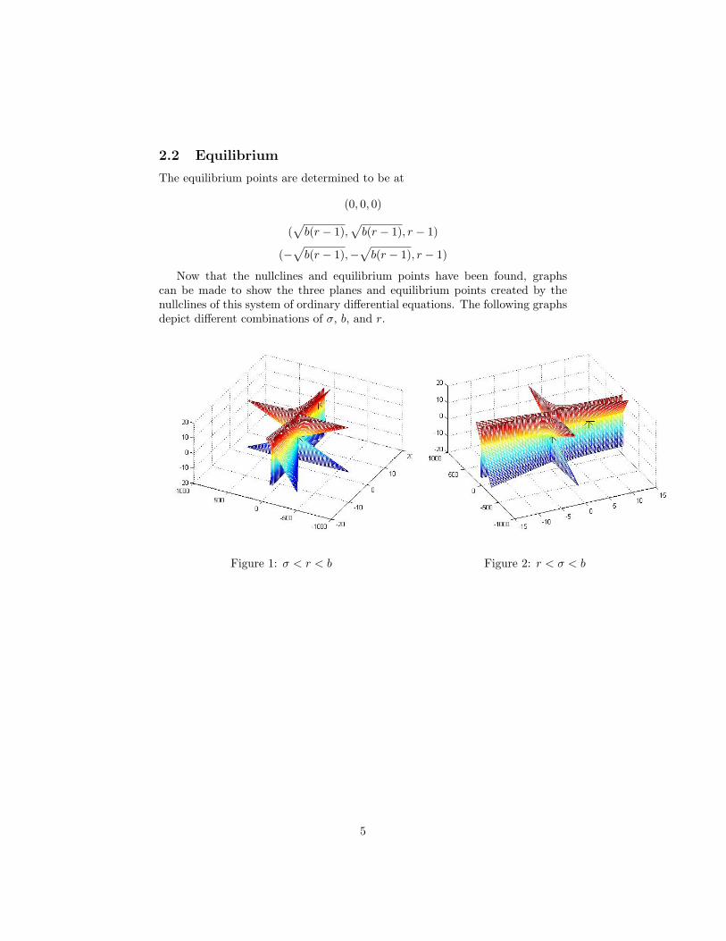
Now that the nullclines and equilibrium points have been found, graphscan be made to show the three planes and equilibrium points created by thenullclines of this system of ordinary differential equations. The following graphsdepict different combinations of σ, b, and r.

Figure 1: σ < r < b Figure 2: r < σ < b

5

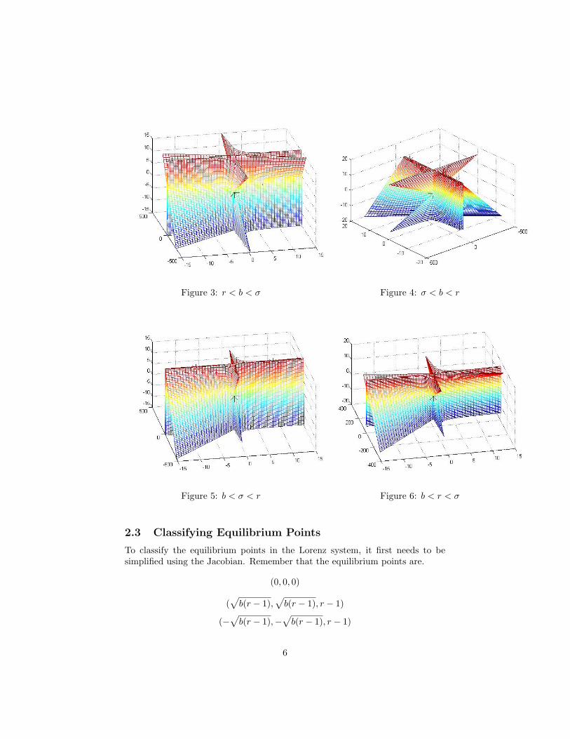
Figure 3: r < b < σ Figure 4: σ < b < r

Figure 5: b < σ < r Figure 6: b < r < σ

2.3 Classifying Equilibrium Points

To classify the equilibrium points in the Lorenz system, it first needs to besimplified using the Jacobian. Remember that the equilibrium points are.

(0, 0, 0)

(√b(r − 1),

√b(r − 1), r − 1)

(−√b(r − 1),−

√b(r − 1), r − 1)

6

The real part of the eigenvalue for the jacobian will determine the classifi-cation of stable or unstable for the certain parameters of σ, b, and r. If all realparts of the eigenvalues are negative, the system is stable. If any of the realparts of the eigenvalues are positive, the system is unstable. When r < 1, thereis only one equilibrium point which is at (0, 0, 0). When this happens, the sys-tem is stable because it converges to zero. The Lorenz system that is intriguingis when r > 470/19. At r > 470/19 the system is unstable. Using Matlab, aprogram can be made to quickly determine the eigenvalues and eigenvector’s forany initial set of conditions σ, b, and r. An example of such a program is in thefollowing link.

This essay isn’t strictly on the Lorenz system, therefore classifications foreach equilibrium point will be based on σ = 10, b = 8/3, and r being varied.

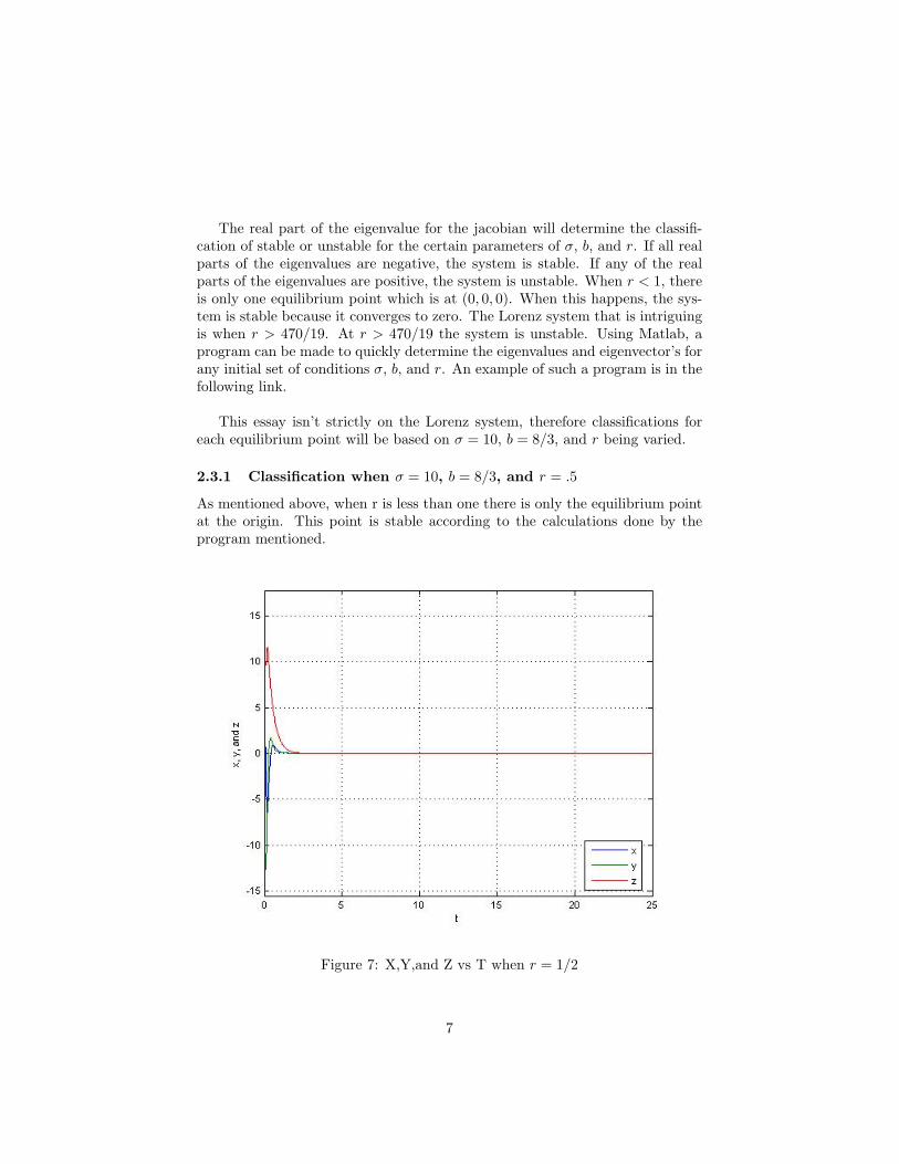
2.3.1 Classification when σ = 10, b = 8/3, and r = .5

As mentioned above, when r is less than one there is only the equilibrium pointat the origin. This point is stable according to the calculations done by theprogram mentioned.

Figure 7: X,Y,and Z vs T when r = 1/2

7

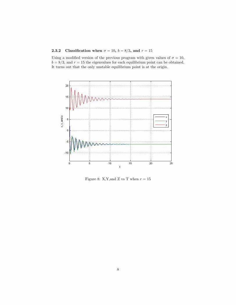
2.3.2 Classification when σ = 10, b = 8/3, and r = 15

Using a modified version of the previous program with given values of σ = 10,b = 8/3, and r = 15 the eigenvalues for each equilibrium point can be obtained.It turns out that the only unstable equilibrium point is at the origin.

Figure 8: X,Y,and Z vs T when r = 15

8

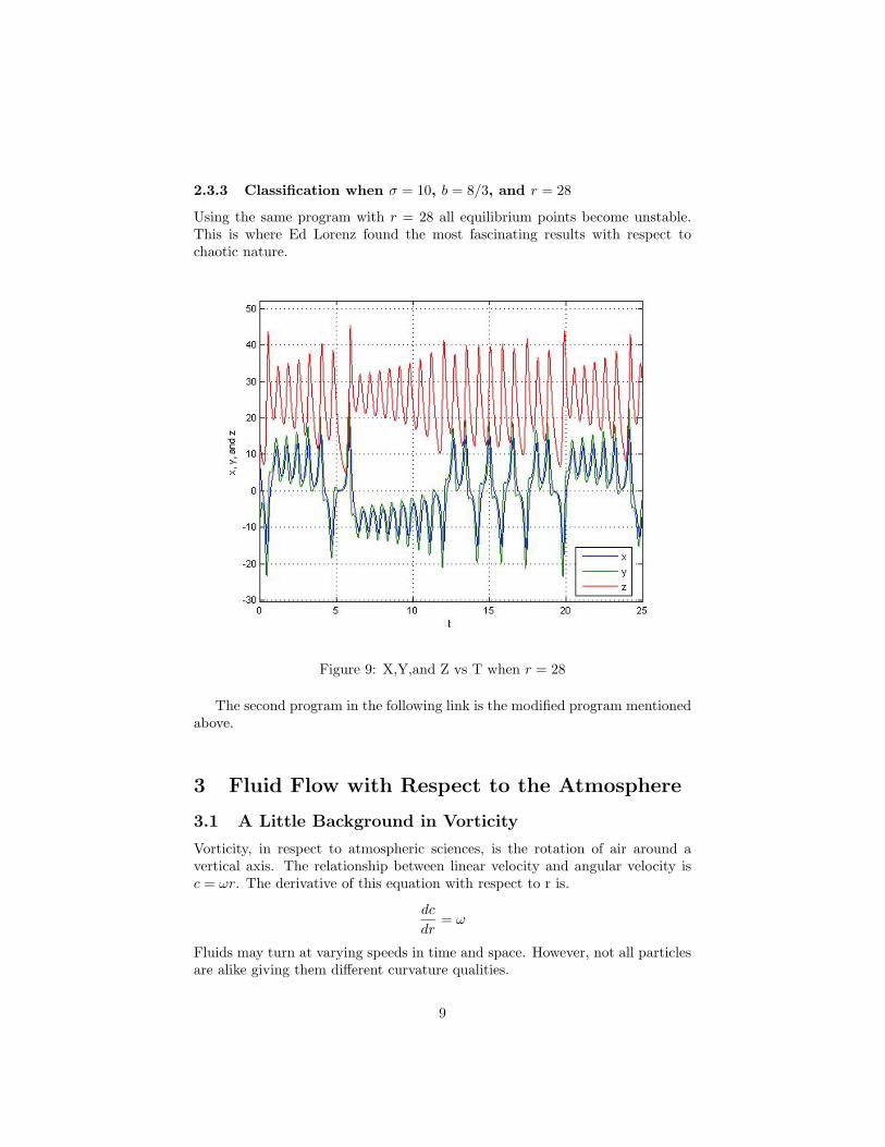
2.3.3 Classification when σ = 10, b = 8/3, and r = 28

Using the same program with r = 28 all equilibrium points become unstable.This is where Ed Lorenz found the most fascinating results with respect tochaotic nature.

Figure 9: X,Y,and Z vs T when r = 28

The second program in the following link is the modified program mentionedabove.

3 Fluid Flow with Respect to the Atmosphere

3.1 A Little Background in Vorticity

Vorticity, in respect to atmospheric sciences, is the rotation of air around avertical axis. The relationship between linear velocity and angular velocity isc = ωr. The derivative of this equation with respect to r is.

dc

dr= ω

Fluids may turn at varying speeds in time and space. However, not all particlesare alike giving them different curvature qualities.

9

If rotation is positive going counterclockwise as in the figure above, then the

Figure 10: Fluid Particles in xy plane

following equations apply.

v = ω1x −u = ω2ydvdx = ω1 −du

dy = ω2

The average between the two angular velocity’s ω1, and ω2 is

12

(ω1 + ω2) =12

(dv

dx− du

dy)

The vorticity is defined as twice the average angular velocity therefore vorticity(ζ)is

ζ =dv

dx− du

dy

10

The earth has it’s own counterclockwise vorticity f = 2Ωsin(θ), therefore wemust add the two to find the absolute vorticity. An example of relative vorticity(ζ) is horizontal wind shear even though it flows in a linear manner.

4 A Little Weather Modeling

In the book, An Introduction to Dynamic Meteorology, models are created andincluded as MatLab files on a cd. The following are a few of the files with de-scriptions on what is going on.

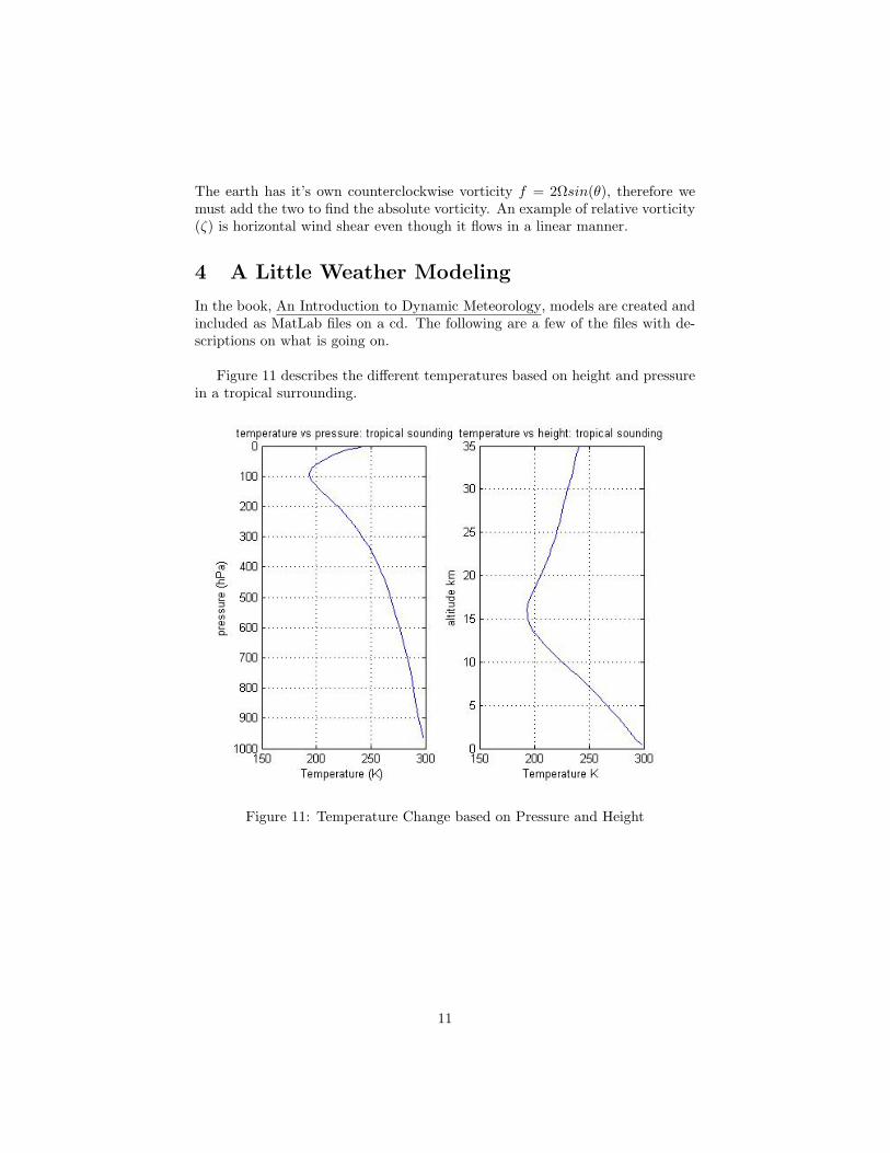
Figure 11 describes the different temperatures based on height and pressurein a tropical surrounding.

Figure 11: Temperature Change based on Pressure and Height

11

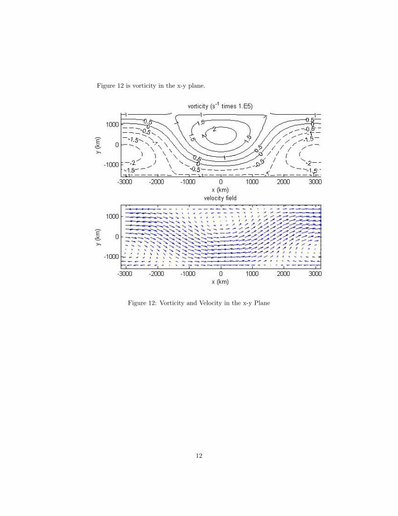
Figure 12 is vorticity in the x-y plane.

Figure 12: Vorticity and Velocity in the x-y Plane

12

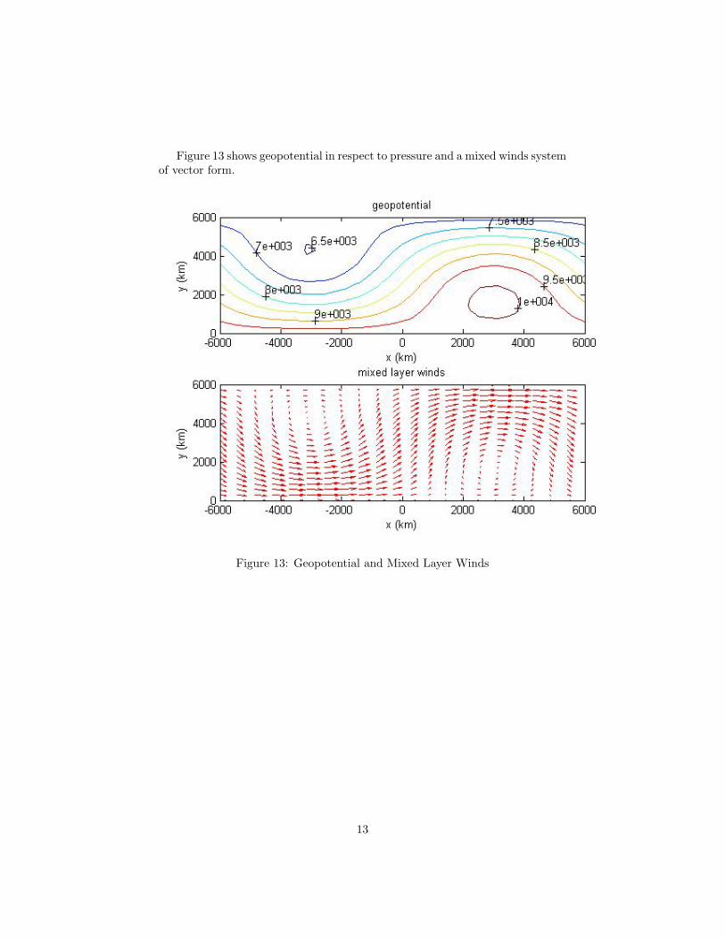
Figure 13 shows geopotential in respect to pressure and a mixed winds systemof vector form.

Figure 13: Geopotential and Mixed Layer Winds

13

Figure 14 shows geostrophic wind along with vorticity for a comparison ofreal particle motion and general wind direction to give a first approximation tomodel wind.

Figure 14: Geostrophic Wind and Vorticity

14

5 Conclusion

The subject of weather and differential equations both partial and ordinary arecontained throughout many works of literature. To condense any of these booksinto an essay would be a feat unimaginable, therefore reading materials in thissubject may provide more understanding and background than the condensedversion presented here. Particularly, An Introduction to Dynamic Meteorologywas an invaluable resource for this project and is actually a text book used inIowa state and the University of Kansas. If a greater understanding of meteo-rology was desired, this book would be highly recommended.There were many partial differential equations that were used to predict theweather on a short time scale but because this essay is based on ordinary differ-ential equations, the partial differential equations were not discussed. Overall,because of the nature of the weather, the numerous factors that come into play,and it’s predictability to be unpredictable it is very difficult to predict weatherover long periods of time. In the future there may be better methods to wherepredictions could be made months ahead of time.

15

References

[1] ”Ordinary Diferential Equations Chaos.” astro.uk. 1 Apr 2009¡http://www.astro.ku.dk/comp-phys/Notes/10.pdf¿

[2] Byers, Horace Robert. General Meteorology. 4. New york: McGraw-HillBook Company, 1974. Print.

[3] Polking, John, Albert Boggess, and David Arnold. Differential Equationswith Boundary Value Problems. 2nd ed. New Jersey: Pearson Education,Inc., 2005. Print.

[4] Hayes, Brian. ”Calculating the weather.(Book review).” Amer-ican Scientist 95.3 (May-June 2007): 271(3). General One-File. Gale. Flathead Valley Community College. 25 Apr. 2009¡http://find.galegroup.com/ips/start.do?prodId=IPS¿.

[5] Holton, James R.. An Introduction to Dynamic Meteorology. 4. San Diego:Elsevier Academic Press, 2004. Print.

[6] Hurricane Andrew [Online image] Available

<http://rsd.gsfc.nasa.gov/rsd/images/andy_lg.jpg, Aug 25 1992>

16