applications of compressive sensing to direction of ... · direction of arrival (doa) estimation of...
TRANSCRIPT

Doctoral Thesis
Applications of CompressiveSensing to Direction of Arrival
Estimation
Mohamed Ibrahim
Dissertation zur Erlangung desakademischen Grades Doktor-Ingenieur (Dr.-Ing.)
Anfertigung im: Fachgebiet Elektronische Messtechnik & Signal Verarbeitung
Institut fur Informationstechnik
Fakultat fur Elektrotechnik und Informationstechnik
Gutachter: Univ.-Prof. Dr.-Ing. Giovanni Del Galdo
Prof. Dr.-Ing. Joao Paulo Carvalho Lustosa da Costa
Prof. Dr. Ahmed El-Sayed El-Mahdy
Vorgelegt am: 02.07.2018Verteidigt am: 28.11.2018
urn:nbn:de:gbv:ilm1-2018000490


Abstract
Direction of Arrival (DOA) estimation of plane waves impinging on an array of sensors
is one of the most important tasks in array signal processing, which have attracted
tremendous research interest over the past several decades. The estimated DOAs are
used in various applications like localization of transmitting sources, massive MIMO
and 5G Networks, tracking and surveillance in radar, and many others. The major
objective in DOA estimation is to develop approaches that allow to reduce the hardware
complexity in terms of receiver costs and power consumption while providing a desired
level of estimation accuracy and robustness in the presence of multiple sources and/or
multiple paths.
Compressive sensing (CS) is a novel sampling methodology merging signal acquisition
and compression. It allows for sampling a signal with a rate below the conventional
Nyquist bound. In essence, it has been shown that signals can be acquired at sub-
Nyquist sampling rates without loss of information provided they possess a sufficiently
sparse representation in some domain and that the measurement strategy is suitably
chosen. CS has been recently applied to DOA estimation, leveraging the fact that a
superposition of planar wavefronts corresponds to a sparse angular power spectrum.
This dissertation investigates the application of compressive sensing to the DOA esti-
mation problem with the goal to reduce the hardware complexity and/or achieve a high
resolution and a high level of robustness. Many CS-based DOA estimation algorithms
have been proposed in recent years showing tremendous advantages with respect to the
complexity of the numerical solution while being insensitive to source correlation and
allowing arbitrary array geometries. Moreover, CS has also been suggested to be applied
in the spatial domain with the main goal to reduce the complexity of the measurement
process by using fewer RF chains and storing less measured data without the loss of any
significant information.
iii

In the first part of the work, we investigate the model mismatch problem for CS
based DOA estimation algorithms off the grid. To apply the CS framework a very com-
mon approach is to construct a finite dictionary by sampling the angular domain with a
predefined sampling grid. Therefore, the target locations are almost surely not located
exactly on a subset of these grid points. This leads to a model mismatch which deterio-
rates the performance of the estimators. We take an analytical approach to investigate
the effect of such grid offsets on the recovered spectra showing that each off-grid source
can be well approximated by the two neighboring points on the grid. We propose a
simple and efficient scheme to estimate the grid offset for a single source or multiple
well-separated sources. We also discuss a numerical procedure for the joint estimation
of the grid offsets of closer sources.
In the second part of the thesis, we study the design of compressive antenna arrays
for DOA estimation that aim to provide a larger aperture with a reduced hardware
complexity and allowing reconfigurability, by a linear combination of the antenna out-
puts to a lower number of receiver channels. We present a basic receiver architecture of
such a compressive array and introduce a generic system model that includes different
options for the hardware implementation. We then discuss the design of the analog com-
bining network that performs the receiver channel reduction. Our numerical simulations
demonstrate the superiority of the proposed optimized compressive arrays compared
to the sparse arrays of the same complexity and to compressive arrays with randomly
chosen combining kernels.
Finally, we consider two other applications of the sparse recovery and compressive
arrays. The first application is CS based time delay estimation and the other one is
compressive channel sounding. We show that the proposed approaches for sparse recove-
ry off the grid and compressive arrays show significant improvements in the considered
applications compared to conventional methods.
iv


Zusammenfassung
Die Schatzung der Einfallsrichtungen (Directions of Arrival/DOA) mehrerer ebener Wel-
lenfronten mit Hilfe eines Antennen-Arrays ist eine der prominentesten Fragestellungen
im Gebiet der Array-Signalverarbeitung. Das nach wie vor starke Forschungsinteresse in
dieser Richtung konzentriert sich vor allem auf die Reduktion des Hardware-Aufwands,
im Sinne der Komplexitat und des Energieverbrauchs der Empfanger, bei einem vorge-
gebenen Grad an Genauigkeit und Robustheit gegen Mehrwegeausbreitung.
Diese Dissertation beschaftigt sich mit der Anwendung von Compressive Sensing
(CS) auf das Gebiet der DOA-Schatzung mit dem Ziel, hiermit die Komplexitat der
Empfangerhardware zu reduzieren und gleichzeitig eine hohe Richtungsauflosung und
Robustheit zu erreichen. CS wurde bereits auf das DOA-Problem angewandt unter der
Ausnutzung der Tatsache, dass eine Superposition ebener Wellenfronten mit einer win-
kelabhangigen Leistungsdichte korrespondiert, die uber den Winkel betrachtet sparse
ist. Basierend auf der Idee wurden CS-basierte Algorithmen zur DOA-Schatzung vorge-
schlagen, die sich durch eine geringe Rechenkomplexitat, Robustheit gegenuber Quellen-
korrelation und Flexibilitat bezuglich der Wahl der Array-Geometrie auszeichnen. Die
Anwendung von CS fuhrt daruber hinaus zu einer erheblichen Reduktion der Hardware-
Komplexitat, da weniger Empfangskanale benotigt werden und eine geringere Daten-
menge zu verarbeiten und zu speichern ist, ohne dabei wesentliche Informationen zu
verlieren.
Im ersten Teil der Arbeit wird das Problem des Modellfehlers bei der CS-basierten
DOA-Schatzung mit gitterbehafteten Verfahren untersucht. Ein haufig verwendeter An-
satz um das CS-Framework auf das DOA-Problem anzuwenden ist es, den kontinuier-
lichen Winkel-Parameter zu diskretisieren und damit ein Dictionary endlicher Große
zu bilden. Da die tatsachlichen Winkel fast sicher nicht auf diesem Gitter liegen wer-
den, entsteht dabei ein unvermeidlicher Modellfehler, der sich auf die Schatzalgorithmen
auswirkt.
vi

In der Arbeit wird ein analytischer Ansatz gewahlt, um den Effekt der Gitterfehler
auf die rekonstruierten Spektra zu untersuchen. Es wird gezeigt, dass sich die Messung
einer Quelle aus beliebiger Richtung sehr gut durch die erwarteten Antworten ihrer
beiden Nachbarn auf dem Gitter annahern lasst. Darauf basierend wird ein einfaches
und effizientes Verfahren vorgeschlagen, den Gitterversatz zu schatzen. Dieser Ansatz ist
anwendbar auf einzelne Quellen oder mehrere, raumlich gut separierte Quellen. Fur den
Fall mehrerer dicht benachbarter Quellen wird ein numerischer Ansatz zur gemeinsamen
Schatzung des Gitterversatzes diskutiert.
Im zweiten Teil der Arbeit untersuchen wir das Design kompressiver Antennenar-
rays fur die DOA-Schatzung. Die Kompression im Sinne von Linearkombinationen der
Antennensignale, erlaubt es, Arrays mit großer Apertur zu entwerfen, die nur weni-
ge Empfangskanale benotigen und sich rekonfigurieren lassen. In der Arbeit wird eine
einfache Empfangsarchitektur vorgeschlagen und ein allgemeines Systemmodell disku-
tiert, welches verschiedene Optionen der tatsachlichen Hardware-Realisierung dieser Li-
nearkombinationen zulasst. Im Anschluss wird das Design der Gewichte des analogen
Kombinations-Netzwerks untersucht. Numerische Simulationen zeigen die Uberlegenheit
der vorgeschlagenen kompressiven Antennen-Arrays im Vergleich mit dunn besetzten
Arrays der gleichen Komplexitat sowie kompressiver Arrays mit zufallig gewahlten Ge-
wichten.
Schließlich werden zwei weitere Anwendungen der vorgeschlagenen Ansatze disku-
tiert: CS-basierte Verzogerungsschatzung und kompressives Channel Sounding. Es wird
demonstriert, dass die in beiden Gebieten durch die Anwendung der vorgeschlagenen
Ansatze erhebliche Verbesserungen erzielt werden konnen.
vii


Acknowledgments
My years as a Ph.D. student at Ilmenau University have been one of the most defining
moments of my life, during which I grew intellectually and professionally. I would like
to thank many who have contributed in more than one way to this journey.
First and foremost, I would like to express my deepest appreciation and sincerest
gratitude to my advisor and my mentor, Dr. Florian Romer for his continuous support.
I am deeply indebted to him for his enthusiasm, immense knowledge, and kindness that
have greatly influenced me in my Ph.D. years. A superb researcher and mentor, he
taught me how to accumulate my research skills, tapped into my full potential, as well
as build up my confidence step by step in the course of researching. He was always
available to help work out the problems whenever I was stuck. I truly take pride in
working with him. Without him, this work would have never been possible.
I feel so grateful for Prof. Giovanni Del Galdo, who has led me to this EMS family
at the Ilmenau University of Technology since 2013. He has provided me tremendous
help. I owe many thanks to him for his encouragement, patience, and guidance. I have
learned greatly from his remarkable knowledge both academically and personally.
I also thank Prof. Joao Paulo C. Lustosa da Costa and Prof. Ahmed El-Mahdy for
reviewing my thesis. Their valuable comments and discussions helped me achieve the
final version of this thesis.
I would also like to thank all friends, professors and colleagues at the EMS group
for the friendly environment during my stay. It has been a great pleasure working with
you all. I did learn from you a lot.
I have been fortunate to have many friends outside the university, who have helped
me and made my life more enjoyable.
On a more personal note, I wish to dedicate this thesis to my family for their endless
and continuous encouragement throughout my life and my studies. My mother, my wife
and my daughter, I can not thank you enough for your selfless love and unconditional
support, patience, and perseverance over the years. No matter where I am and what I
am doing, you are the love of my life for eternity. To you, I dedicate this work.
ix


Contents
Contents xi
1 Introduction 1
2 Background 7
2.1 Compressive Sensing . . . . . . . . . . . . . . . . . . . . . . . . . . . . . 7
2.1.1 Conventional Sampling . . . . . . . . . . . . . . . . . . . . . . . . 9
2.1.2 Sparsity . . . . . . . . . . . . . . . . . . . . . . . . . . . . . . . . 10
2.1.3 Incoherent Measurements . . . . . . . . . . . . . . . . . . . . . . 12
2.1.3.1 Measurement Matrix Design . . . . . . . . . . . . . . . . 14
2.1.4 Non-Linear Recovery . . . . . . . . . . . . . . . . . . . . . . . . . 17
2.1.4.1 Recovery off the Grid . . . . . . . . . . . . . . . . . . . 19
2.2 Direction of Arrival Estimation . . . . . . . . . . . . . . . . . . . . . . . 21
2.2.1 The Array Signal Model . . . . . . . . . . . . . . . . . . . . . . . 22
2.2.2 Array Processing DOA Estimation Methods . . . . . . . . . . . . 25
2.2.2.1 Spectral Estimation . . . . . . . . . . . . . . . . . . . . 26
2.2.2.2 Parametric Estimation . . . . . . . . . . . . . . . . . . . 28
3 Compressive Sensing Based DOA Estimation off the Grid 31
3.1 Motivation . . . . . . . . . . . . . . . . . . . . . . . . . . . . . . . . . . . 32
3.2 Analytical Study of the Problem . . . . . . . . . . . . . . . . . . . . . . . 34
3.3 An Approximation Scheme for offgrid Sources . . . . . . . . . . . . . . . 35
3.3.1 Single Source . . . . . . . . . . . . . . . . . . . . . . . . . . . . . 35
3.3.2 Multiple Sources . . . . . . . . . . . . . . . . . . . . . . . . . . . 38
3.4 Polarimetric Extension . . . . . . . . . . . . . . . . . . . . . . . . . . . . 41
3.4.1 Polarimetric CS based DOA Estimation . . . . . . . . . . . . . . 42
3.4.2 Polarimetric CS based DOA Estimation on the Grid . . . . . . . . 43
3.4.3 Polarimetric CS based DOA Estimation off the Grid . . . . . . . 43
3.4.4 The Cost Function and its Implementation . . . . . . . . . . . . . 46
3.5 Numerical Results . . . . . . . . . . . . . . . . . . . . . . . . . . . . . . . 48
3.5.1 CS based DOA Estimation off the Grid . . . . . . . . . . . . . . . 48
3.5.2 Polarimetric CS DOA Estimation off the Grid . . . . . . . . . . . 50
3.6 Summary . . . . . . . . . . . . . . . . . . . . . . . . . . . . . . . . . . . 55
xi

CONTENTS
4 Compressive Antenna Arrays for Direction of Arrival Estimation 57
4.1 Motivation . . . . . . . . . . . . . . . . . . . . . . . . . . . . . . . . . . . 574.2 Compressive Arrays . . . . . . . . . . . . . . . . . . . . . . . . . . . . . . 624.3 Design of the Combining Matrix . . . . . . . . . . . . . . . . . . . . . . . 65
4.3.1 Generic Design Approach . . . . . . . . . . . . . . . . . . . . . . 654.3.2 Design Based on the SCF . . . . . . . . . . . . . . . . . . . . . . 664.3.3 Design Based on the CRB . . . . . . . . . . . . . . . . . . . . . . 69
4.4 Adaptive Focusing Design . . . . . . . . . . . . . . . . . . . . . . . . . . 714.5 Estimation Quality . . . . . . . . . . . . . . . . . . . . . . . . . . . . . . 744.6 Numerical Results . . . . . . . . . . . . . . . . . . . . . . . . . . . . . . . 76
4.6.1 Performance Analysis of the SCF Based Design . . . . . . . . . . 764.6.2 Comparison to the CRB Based Design and Sparse Arrays . . . . . 824.6.3 Performance Analysis for Adaptive Focusing . . . . . . . . . . . . 89
4.7 Summary . . . . . . . . . . . . . . . . . . . . . . . . . . . . . . . . . . . 95
5 Compressive Time Delay Estimation 97
5.1 Motivation . . . . . . . . . . . . . . . . . . . . . . . . . . . . . . . . . . . 975.2 Time Delay Estimation . . . . . . . . . . . . . . . . . . . . . . . . . . . . 1005.3 Compressive Sampling TDE Architecture . . . . . . . . . . . . . . . . . . 1015.4 Delay Estimation Procedure . . . . . . . . . . . . . . . . . . . . . . . . . 104
5.4.1 Gridded Sparse Recovery Based Estimator . . . . . . . . . . . . . 1045.4.2 Correlation Based Estimator . . . . . . . . . . . . . . . . . . . . . 105
5.5 Measurement Design . . . . . . . . . . . . . . . . . . . . . . . . . . . . . 1055.6 Compressive RBS Synchronization . . . . . . . . . . . . . . . . . . . . . . 1075.7 Numerical Results . . . . . . . . . . . . . . . . . . . . . . . . . . . . . . . 110
5.7.1 Compressive Time Delay Estimation . . . . . . . . . . . . . . . . 1115.7.2 Compressive RBS Synchronization . . . . . . . . . . . . . . . . . 113
5.8 Summary . . . . . . . . . . . . . . . . . . . . . . . . . . . . . . . . . . . 115
6 Compressive Spatial Channel Sounding 117
6.1 Motivation . . . . . . . . . . . . . . . . . . . . . . . . . . . . . . . . . . . 1176.2 Channel Sounding . . . . . . . . . . . . . . . . . . . . . . . . . . . . . . . 1196.3 Compressive Spatial Channel Sounding . . . . . . . . . . . . . . . . . . . 1216.4 Numerical Simulations . . . . . . . . . . . . . . . . . . . . . . . . . . . . 1246.5 Summary . . . . . . . . . . . . . . . . . . . . . . . . . . . . . . . . . . . 128
7 Conclusions 131
Bibliography 154
xii

Chapter 1
Introduction
The introduction of mobile and wireless communication systems in the late 20th cen-
tury has radically changed the life of human beings. In a few years time, the wireless
communications industry has grown to become one of the largest in the world. The
markets show significant growth, and the volumes are high. According to the Ericsson
mobility report 2017 [14], the estimated amount of subscribers in 2017 is 7.8 billion,
while the expected amount of subscribers for 2023 is 9.1 billion. Moreover, the total
mobile data traffic is expected to increase to almost seven times. In addition to the
more traditional services such as speech, texting, and video, wireless communication
systems can also provide other services to improve the quality of life, including health
care, home automation, emergency services and many others.
Since the early days of wireless communication, the simple single antenna has been
used to transmit and receive wireless signals. In order to improve the effectiveness of
a wireless communication system, an array of antennas can be used to transmit and
receive. An antenna array consists of a set of antennas that are located at different
points in space with reference to a common reference point. These sensors listen to the
incoming signals and provide a means of sampling these signals in space. Compared
to single sensor systems, array systems have some crucial advantages. A significant
advantage is signal enhancement over noise by appropriate processing of the received
signals. Moreover, it allows spatial selection of where to transmit power. This boosts the
range of the communication link by focusing the power toward a certain user rather than
radiating energy in all directions. Spatial selection also enables frequency reuse, which
means that the same frequency can be used by multiple nodes by spatially discriminating
between them [15]. Similarly, sensor arrays can be used to monitor the position of a
source by tracking its signature as it moves in space.
1

Chapter 1 Introduction
The sensor array data is then processed to extract useful information. This corre-
sponds to either the content of the signal itself as often found in communications or some
parameters related to the recorded data. Array signal processing is used in several appli-
cation areas such as radar, sonar, wireless communications, radio astronomy, seismology,
acoustics, and medical imaging [16,17]. Early contributions to this field have been made
mostly in the context of wireless communications and radar systems in the first half of
the 20th century. In the second half of the 20th century, the tremendous progress of
digital processing hardware led to numerous new developments and applications [18].
A typical objective of array signal processing is to estimate the direction-of-arrival
(DOA) of an incoming signal. Through the collection of received time samples and by
processing of spatial signals, detection of multiple incoming sources and estimation of
their DOAs can be realized [19]. The estimated DOAs are used in various applications
like localization of transmitting sources, for direction finding [20,21], massive MIMO and
5G Networks [21,22], channel sounding and modeling [23–26], tracking and surveillance
in radar [27], and many others. The major objective in DOA estimation is to develop
approaches that allow minimizing the hardware complexity in terms of receiver costs and
power consumption while providing a desired level of estimation accuracy and robustness
in the presence of multiple sources and/or multiple paths.
Research on DOA estimation using array processing has largely focused on uniform
arrays (e.g., linear and circular) [28] for which many efficient parameter estimation
algorithms have been developed. The main goal is to locate closely spaced signals
in angle, in the presence of high-variance noise and a low number of snapshots. To
perform well, all such algorithms require to fulfill certain conditions on the sampling of
the wavefront of the incident waves in the spatial domain. Namely, the distance between
adjacent sensors should be less than or equal to half a wavelength of the impinging planar
wavefronts; otherwise it leads to grating lobes (sidelobes) in the spatial correlation
function which correspond to ambiguities in the array manifold. At the same time,
to achieve DOA estimation with a high resolution, the receiving arrays should have a
relatively large aperture. This implies that arrays with a large number of antennas are
needed to obtain a high resolution, which is not always feasible.
It was shown in [29] that if the field is modeled as a superposition of a few planar
wave-fronts, the DOA estimation problem can be expressed as a sparse recovery problem
and the Compressed Sensing (CS) framework can be applied. Compressive Sensing (CS)
[30–32] is a novel paradigm in sampling theory that provides an analytical framework
for the sampling of signals below the Shannon-Nyquist sampling rate. In essence, it has
been shown that signals can be acquired at sub-Nyquist sampling rates without loss of
2

information provided they possess a sufficiently sparse representation in some domain
and that the measurement strategy is suitably chosen. In particular, guarantees for
recovering the signal from a certain number of linear measurements have been derived
which have also led to insights on how to determine applicable measurement designs.
Recently, compressive sensing has been widely studied and applied to various fields, such
as imaging [33,34], magnetic resonance imaging [35,36], video processing [37,38], radar
[39–41], analog-to-information conversion [42], sensor networks [43,44], array processing
[45], communications [46, 47], astronomy [48, 49] and biology [50].
Many powerful CS-based DOA estimation algorithms have been proposed in recent
years showing tremendous advantages with respect to the hardware complexity of the
receiving arrays and the complexity of the numerical solution while being insensitive
to source correlation and allowing arbitrary array geometries. However, they all face
a common problem. Although the model is sparse in a continuous angular domain, to
apply the CS framework we need to construct a finite dictionary by sampling this domain
with a predefined sampling grid i.e., the angle space is divided into a large number of
grids where the source directions of interest are assumed to exactly lie on some of the
grids. However, the target locations in practice are almost surely not located exactly
on a subset of these grid points. This leads to a model mismatch that results in the
degradation of the performance.
Compressed sensing has also been suggested to be applied in the spatial domain
(e.g., array processing and radar) with the main goal to reduce the complexity of the
measurement process by using fewer RF chains and storing less measured data without
the loss of any significant information. In particular, the CS paradigm can be applied
in the spatial domain by employing N antenna elements that are combined using an
analog combining network to obtain a smaller number of M < N receiver channels.
Since only M channels need to be sampled and digitized, the hardware complexity
remains comparably low (e.g., consuming less energy and storing less data) while a
larger aperture is covered which yields a better selectivity than a traditional, Nyquist
(λ/2) spaced M-channel antenna array.
The objective of this dissertation is threefold. Firstly, CS based DOA estimation
methods exploring sparsity will be studied with the main goal to lift the off-grid model
mismatch. We study the problem analytically and propose an efficient CS based DOA
estimation technique that works with off-grid sources. Secondly, we propose a com-
pressive array for DOA estimation with a lower hardware complexity and an optimized
design for the compressive network. Thirdly, we consider two other applications of the
sparse recovery and compressive arrays. The first application is CS based time delay
3

Chapter 1 Introduction
estimation and the other one is compressive channel sounding. We show that the pro-
posed approaches for sparse recovery off the grid and compressive arrays show significant
improvements in the considered applications compared to conventional methods.
Overview and Contributions
The work in this thesis is organized as follows:
Chapter 2 provides the theoretical background for the main topics covered in this
thesis namely, compressed sensing (CS) and direction of arrival (DOA) estimation. It
starts with a review of the CS theory and its fundamentals, with the aim of providing
a summarized, yet a standalone background to this thesis. The fundamentals of DOA
estimation are then presented where first the array design essentials are reviewed and
then parameter estimation techniques are discussed and summarized. While no novel
material is presented in this chapter, its role is essential in agreeing on the notation and
concepts addressed in the rest of this work.
Chapter 3 deals with the problem of applying CS techniques to DOA estimation
off the grid. We take an analytical approach to investigate the effect of recovering the
spectrum of sources not lying on the grid. Unlike earlier works that have provided
a quantitative analysis of the approximation error, we examine the specific shape of
the resulting spectrum. We show that for one off-grid source the recovered spectrum
is not sparse but it can be well approximated by the closest two dictionary atoms on
the grid and their coefficients can be exploited to estimate the grid offset. We then
extend our model to consider multiple sources. In the second part of the chapter, a full
polarimetric CS based DOA estimator (also off the grid) is proposed. Almost all CS
based DOA estimation techniques consider a non-polarimetric model which can lead to
entirely useless estimation results. We show that our polarimetric CS based model can
estimate both the DOA and the polarization state of each individual path with very
high accuracy. The results shown in this chapter have been published in [1–3].
Chapter 4 discusses the design and the performance of compressive arrays employ-
ing linear combinations in the analog domain by means of a network of power splitters,
phase shifters, and power combiners. We present a basic receiver architecture of such a
compressive array and introduce a generic system model that includes different options
for the hardware implementation. Importantly, the model reflects the implications for
the noise sources. Based on the generic system model we then discuss the design of the
combining matrix, with the goal to obtain an array that is suitable for DOA estimation
(i.e., minimum variance of DOA estimates and robustness in terms of low side lobe levels
4

or low probability of false detections). We propose two design approaches. The first is
based on the spatial correlation function which is a low-complexity scheme that in cer-
tain cases even admits a closed-form solution. The second is based on the minimization
of the Cramer-Rao Bound (CRB). We show by numerical simulations that both of the
proposed design approaches have a significant performance improvement compared to
the state of the art, namely an array with a randomly chosen combining matrix and a
sparse array with optimized sensor positions. The results proposed in this chapter are
published in [4–9].
Chapter 5 extends the ideas from the previous chapters applying them to time delay
estimation (TDE) and synchronization. We first treat the special case of estimating the
delay of a signal with a known pulse shape from a noisy superposition of several delayed
copies. The main contribution of the first part of the chapter is an optimization based
design for the measurement kernels of the CS based TDE architectures. We demonstrate
numerically that the proposed optimized CS kernels outperform a randomly chosen
one in terms of the delay estimation accuracy. In the second part of the chapter, we
turn our attention to synchronization of the TDE network. We proposed a CS based
reference broadcast synchronization where the reference signal is an opportunistic signal
already in the system (e.g., FM or TV signals). We show that using CS, the correlation
can be calculated in the compressed domain, yet achieving a correlation characteristics
comparable to the high bandwidth correlation obtained with opportunistic signals. The
ideas discussed in this chapter have been published in [10–12].
Chapter 6 exploits the application of CS to the double-directional channel sounder
in the spatial domain that includes joint DOA/DOD estimation. Extending the ideas
of compressive arrays discussed in Chapter 4, a compressive spatial channel sounder is
proposed and evaluated based on real scenarios showing superior advantages in terms of
time, hardware complexity and resolution. In particular, the proposed approach reduces
the total number of switching periods, which implies a reduced channel acquisition time
and thus an improved Doppler bandwidth. On the other hand, the compressive approach
reduces the number of RF chains, which is a very relevant advantage in terms of the
overall receiver complexity, the amount of data to be processed in the digital domain
(e.g., FPGA), power consumption, as well as RF hardware calibration. Alternatively, for
the same measurement time and/or hardware complexity, one can increase the number
of array elements to cover a larger aperture and so achieving better performance in
terms of resolution. The ideas presented in this chapter are published in [13].
Chapter 7 concludes the work presented and summarizes the main contributions of
this thesis providing directions for future work.
5

Chapter 1 Introduction
6

Chapter 2
Background
This chapter overviews some background of the two main topics related to the research
contributions presented in this thesis: Compressive Sensing (CS) and Direction of Arrival
(DOA) estimation. In Section 2.1, the CS theory is first reviewed where the underlying
principles are presented and the main concepts are explained. Afterwards, we turn our
attention to the DOA estimation problem using antenna arrays in Section 2.2. We start
by deriving the array signal model and then the main parameter estimation techniques
used for DOA estimation are discussed and compared. Due to the large volume of
existing literature, the chapter here is only directly related to the current thesis and is
by no means a complete treatment of all past work.
2.1 Compressive Sensing
We live in an analog world. Most natural phenomena are the representation of vari-
ations in physical quantities in any given time. These parameters include electricity,
temperature, light, sound and pressure among others. With the invention of transistors
and microprocessors around 1950, the digital revolution started and it was reported in
2014 that more than 99% of the world’s technologically stored information is in digital
format [51]. Digital technology allows information to be copied and replicated precisely.
It is due to digital technology that our society is now so defined by computers, smart-
phones, internet access, and cell phone communication. The Digital Revolution, in fact,
marks the beginning of a new age: the Information Age [52].
To go from analog to digital, we rely on two main principles: sampling and quanti-
zation. This conversion is achieved via an Analog-to-Digital Converter (ADC), which is
an electronics component present in any digital device that processes an analog input
signal. The ADC converts an analog signal to a discrete time signal and a discrete
7

Chapter 2 Background
amplitude signal. Through sampling, the ADC transforms the continuous signal with
an infinite number of possible values to a finite number of samples. Furthermore, the
ADC must quantize the input signal, meaning that every sample must be represented
by a value from a finite set of possible values [53].
Sampling theorems provide conditions required for lossless conversion between the
continuous and the discrete-time worlds for digital signal processing. For many years,
signal processing has been relying on the well-known Nyquist/Shannon sampling theo-
rem [54,55], stating that the sampling rate must be at least twice as high as the highest
frequency to avoid losing information while capturing the signal.
Such strategy faces difficulties in the acquisition of wideband signals where the re-
quired sampling rates exceed the limits of state-of-art commercial ADC systems. The
hardware implementation of devices to obtain such high resolution (in image acquisition
for example) requires very complex designs with very high costs. Moreover, it might not
be possible to store all the data because of limited storage, or the data amount might
be too large to be processed so that it becomes necessary to apply compression methods
to get rid of the redundant information and keep the minimum information required
for almost perfect reconstruction [56]. This means that very complex ADC devices are
deployed to acquire samples of the signal and then compression techniques are applied
to dump most of these samples since only a few of them are significant for recovery.
In [57] the authors show that it is possible to lower the necessary sampling rate and
still attain a desired level of information if the information rate is much lower than the
actual signal dimensionality. For example, an image of a million pixels has a million
degrees of freedom. However, a typical image is very sparse or compressible over the
wavelet basis, namely, very likely only a small fraction of wavelet coefficients, say, one
hundred thousand out of a million wavelet coefficients, are significant in recovering the
original images, while the rest of wavelet coefficients are discarded in many compression
algorithms.
In the last decade, a new theory of compressive sensing (CS), also known under the
terminology of compressed sensing or compressive sampling, has considerably drawn the
attention of researchers. It builds a fundamentally novel approach to data acquisition
and compression which overcomes drawbacks of the traditional method. In his famous
paper [30], Donoho posed the ultimate goal of merging compression and sampling. In-
stead of acquiring all the signal data to through it away afterwards, it was suggested to
directly measure the part that will not end up being thrown away. This was the funda-
mental idea for which the field of compressive sensing has emerged. In 2006, Donoho,
Candes, Romberg and Tao [30–32] conducted a series of in-depth research based on the
8

2.1 Compressive Sensing
discovery that a signal may still be recovered even though the number of data is deemed
insufficient by Shannon’s criterion, and built the theory of compressive sensing. Instead
of acquiring this large number of samples and then compressing them, obtain only these
few non-zero coefficients directly. In other words, compress the data while sampled.
Recently, compressive sensing has been widely studied and applied to various fields,
such as imaging [33, 34], magnetic resonance imaging [35, 36], video processing [37, 38],
radar [39–41], analog-to-information conversion [42], sensor networks [43,44], array pro-
cessing [45], communications [46, 47], astronomy [48, 49] and biology [50].
In this section, we will display the main theoretical results of the compressive sens-
ing paradigm together with the main underlying principles. We start in Section 2.1.1
by briefly describing the traditional sampling approach. Afterwards, we discuss the
three main principles underlying the CS theory: sparsity in Section 2.1.2, incoherent
measurements in Section 2.1.3 and sparsity based non-linear recovery in Section 2.1.4.
2.1.1 Conventional Sampling
Figure 2.1 shows the process of conventional Nyquist-Rate sampling. A source emits a
signal x ∈ CN×1 which is an N dimensional complex signal. In the noiseless case, N
linear measurements y ∈ CN×1 are taken using an N × N measurement ensemble Φ,
i.e.,
y = Φ · x. (2.1)
Afterwards, the obtained signal y can be analyzed and processed digitally where
traditional compression techniques (e.g., JPEG [58]) can be applied to get rid of the
redundancy and keep only the M < N significant coefficients sufficient for the signal’s
recovery.
PSfrag replacements
x ∈ RN
Source Nyquist-RateSampling
y ∈ RNAnalysis &Compression
y ∈ RM
Figure 2.1: Conventional Nyquist-Rate Sampling
Conventional Nyquist-Rate sampling suggests that N linearly independent measure-
ments are required for the exact recovery of an arbitrary signal x. The matrix Φ should
be a square matrix that has a full rank, i.e., its columns are linearly independent and
span an N dimensional subspace. Therefore, it can be used to represent all possible
signals in CN and each signal has one unique representation. In such a case, if y and
9

Chapter 2 Background
Φ are given and Φ has full rank, x can be obtained by solving the system of linear
equations, which is equivalent to multiplying y with the inverse of Φ denoted Φ−1.
If M < N measurements are taken, the problem becomes underdetermined and the
measurement cannot be uniquely inverted. This is where the CS theory comes into play
suggesting the possibility to solve such an ill-posed, underdetermined problem promising
to reconstruct a signal accurately and efficiently from a set of a few non-adaptive linear
measurements M ≪ N . Figure 2.2 shows the CS scheme. The compressed signal
y ∈ RM can be directly acquired from the signal of interest x ∈ RN via an M × N
compressive measurement ensemble Φ. To get back the original signal x from the
compressed signal y, non-linear recovery techniques are employed.
PSfrag replacements
s(t)Source Compressive
Sampling
y ∈ RMNon-LinearRecovery
x ∈ RN
Figure 2.2: Compressive Sensing Architecture
In this sense, the CS theory counts on three key elements: sparsity (Section 2.1.2),
incoherent measurements (Section 2.1.3) and non-linear recovery (Section 2.1.4). Spar-
sity screens out the signal of interest, while incoherence restricts the sensing schema.
Specifically, a large but sparse signal s(t) is encoded by a relatively small number of
incoherent linear measurements y ∈ RM . Using non-linear recovery algorithms, the orig-
inal signal can be reconstructed from the encoded sample by finding the sparsest signal
from the solution set of an underdetermined linear system. Each of these principles is
comprised of a dense, rapidly evolving literature of which only the fundamentals are
reviewed in the following sections of this chapter as a basic background for this thesis.
2.1.2 Sparsity
Sparsity is the signal structure behind many compression algorithms that employ trans-
form coding and is the most famous signal structure used in CS.
Definition 1. The ℓp-norm of a vector signal x is defined as
‖x‖p =( N∑
n=1
‖xn‖p)(1/p)
for p ≥ 1. (2.2)
At times a quasinorm such as ℓ0 is also used, which cannot be used in the above
10

2.1 Compressive Sensing
formula, but which corresponds only to counting all the non-zero entries in the vector
x.
Definition 2. A signal x ∈ CN×1 is said to be K-sparse for some K ∈ N, if at most K
of its entries are non-zero, i.e., if ‖x‖0 ≤ K.
The use of sparsity as a model for signal processing dates back to Donoho and
Johnstone’s initial works in the early 1990s [59], where wavelet-sparse signals and images
were denoised by assuming that the noiseless version of the signal is sparse. Since then,
many mathematicians, applied mathematicians, and statisticians have employed sparse
signal models for applications that include signal enhancement and super resolution,
signal deconvolution, and signal denoising [60].
Sparse representations are the core tenet of compression algorithms based on trans-
form coding. In transform coding, a sparse signal x is compressed by obtaining its
sparse representation s in a suitable basis Ψ and encoding the values and locations of
its nonzero coefficients. Transform coding is the foundation of most commercial com-
pression algorithms; examples include the JPEG image compression algorithm, which
uses the discrete cosine transform [58], and the JPEG2000 algorithm, which uses the
discrete wavelet transform [61].
While transform coding algorithms are able to encode sparse signals without distor-
tion, the signals that we observe in nature are not exactly sparse, but rather compress-
ible.
Definition 3. For a signal x ∈ CN×1, some K ∈ N and some p ≥ 1, we define the
K-term approximation error of x with respect to the p-norm as
σK(x)p := minx∈ΣK
‖x− x‖p, (2.3)
where Σ denotes the set of all K-sparse vectors ∈ CN×1.
A signal is called compressible if there exists a good K-term approximation xK
with a fast decaying approximation error σK for some p ≥ 1, i.e., most of its energy is
concentrated around no more than K entries.
While a widely accepted standard, the sample-then-compress ideology behind trans-
form coding compression suffers from three inherent inefficiencies: First, we must start
with a potentially large number of samples N even if the ultimate desired K is small.
Second, the encoder must compute all of the N transform coefficients s, even though it
will discard all but K of them. Third, the encoder faces the overhead of encoding the
locations of the large coefficients.
11

Chapter 2 Background
One would think intuitively to acquire just a few linear measurements proportional
to the signal sparsity K. This is indeed correct, but the difficulty is determining in
which lower dimensional subspace such a signal lies [62]. That is, we may know that the
signal has a few non-zero coordinates, but we do not know which coordinates those are.
It is thus clear that we may not reconstruct such signals using a simple linear operator,
and that the recovery requires more sophisticated techniques.
2.1.3 Incoherent Measurements
Assume now that x is sparse in a domain Ψ, where Ψ is an N ×N basis matrix. This
means that x has only K non-zero elements with K ≪ N . If the positions of the
non-zero coefficients of x were known in advance, we could reconstruct it from exactly
K linear measurements, i,e, each row of Φ can be set to zero everywhere but at the
position of a non-zero entry of x.
This is exactly where the theory of CS comes into play. It introduces measurement
and reconstruction strategies so that M ≪ N linear measurements are sufficient for
exact reconstruction of K-sparse signals where K ≤ M . The CS measurement process
can be described as a linear projection of the signal vector into a set of carefully chosen
projection vectors that gathers all (or most of) the information contained in the signal.
Each measurement of a signal should give some global information. With incoherent
measurements, every measurement gives a little bit of information that adds up to give
the whole information content of the signal of interest [63].
The measurement matrix Φ is then a “fat” matrix with much fewer rows than
columns, and the system(2.1) is massively underdetermined with infinitely many so-
lutions. The matrix does not constitute an isometry for all input vectors x. However,
near-isometry is possible if only a subset of input vectors is allowed, which is the case
when assuming only sparse signals.
Definition 4. A matrix Φ ∈ CM×N is said to satisfy the restricted isometric property
(RIP) of order K ∈ N, if there exists a constant 0 ≤ δ < 1 such that
(1− δK)‖x‖22 ≤ ‖Φ · x‖22 ≤ (1 + δK)‖x‖22 (2.4)
holds for every K-sparse x ∈ ΣK.
The smallest such constant is denoted by σK , and is called the restricted isometric
constant (RIC) of Φ. If the RIC of a matrix Φ is small (i.e., as close to 0 as possible),
the restriction of Φ to any subset of K columns behaves analogously like an isometry.
12

2.1 Compressive Sensing
This theorem is very important because it means that if a matrix Φ can be found that
satisfies the RIP of order 2K, it will approximately preserve the distance between any
pair of K-sparse input vectors with respect to some constant σK .
It is important to mention that testing this property for a generic sensing matrix
requires the computation of the singular values of all its(NK
)-column submatrices, and
is non-deterministic polynomial-time (NP)-hard [64], which makes it practically not
feasible to design an appropriate measurement matrix based only on this criteria.
Another method to assess the information-preserving properties of sensing matrices
is the coherence (also mutual coherence) which can be defined as follows [65]
Definition 5. The coherence of a matrix Φ, µ(Φ), is the largest inner product between
any columns φi,φj of Φ:
µ(Φ) = max1≤i<j≤N
∣∣φH
i · φj
∣∣
‖φi‖2 · ‖φj‖2. (2.5)
In fact, it is possible to relate the RIP property and the coherence [66], but they
can give different insights about the measurement ensemble. Coherence is essentially
an index of linear dependence between the columns of Φ and should be made as small
as possible as to guarantee the recoverability of sparse vectors. Contrarily to the RIP,
coherence, however, has the benefit of being computable on any instance of Φ, and is
also related to the performances of many signal recovery algorithms [65]. It is therefore
recommended as a figure of merit that should be made as small as possible to guarantee
that a generic Φ allow for the recovery of a sparse vector x.
The next question therefore is, which matrices satisfy the RIP and/or the coherence
conditions to ensure informative sensing. Such matrices should be non-adaptive, i.e.,
independent of the sparse dictionary Ψ. In 2006 though, the groundbreaking work of
Candes, Romberg and Tao [31, 32] and Donoho [30] came to the rescue. By using the
concept of randomness, they were able to define a class of matrices that, with very
high probability, will satisfy the RIP and enjoy low coherence properties. Since then,
many such classes of matrices have been identified and proven to satisfy the required
conditions [67, 68].
For example, consider Gaussian random matrices, i.e. matrices where the entries
are identically and independently distributed Gaussian random variables with mean
0 and variance 1/M , or Bernoulli random matrices, where the entries take the value
+1/√
(M) or −1/√
(M) with equal probability. It can be shown that such matrices
satisfy the RIP of some order K with small RIC σK with very high probability if the
number of rows is chosen large enough [67]. In many of the theory-building work in
13

Chapter 2 Background
CS, Gaussian or Bernoulli random matrices are used. In practice, though, they are
of limited use for several reasons. For example, in some applications, the design of
the measurement matrix is constrained by physical or other conditions. Also, these
matrices do not allow a fast matrix multiplication, which typically has to be performed
quite often in practical applications. Therefore, structured random matrices are often
preferred [44, 69]. In the following subsection, we review state-of-the-art measurement
matrix design for compressive sensing.
2.1.3.1 Measurement Matrix Design
So far many of the CS schemes employ the Gaussian or Bernoulli matrix for their
measurement matrix design or optimization. However, as proposed in [70], the Gaussian
random matrix, typically used in the CS problems, is not necessarily the best choice for
a given basis matrix in terms of the coherence of column pairs in the sensing matrix.
Furthermore, in many applications, it is difficult for designers to generate and control a
perfect Gaussian random matrix in physical electric circuit with its randomness being
well guaranteed. Moreover, there is no efficient algorithm testing the RIP of a random
matrix, even though it does satisfy the RIP with overwhelming probability. The question
to be asked next, therefore, is whether we can do better than random. Do there exist
principled and mathematically founded ways to find matrices that are ’optimal’, in some
sense, for recovery using compressive sensing methods?
Compared with random sensing matrices, deterministic ones can get rid of these
drawbacks. They can be generated on the fly to save storage space and the RIP is often
easy to verify. In addition, by exploiting specific structures of deterministic matrices,
fast algorithms can be designed to enhance the efficiency of recovery. Many efforts
indeed have been excelled to model the way the samples are acquired in practice, which
leads to sensing matrices that inherit their structure from the real world.
Early efforts were trying to implement such random measurement ensembles practi-
cally. An early trial to implement random compressive measurements is the so called
random filter [71]. The approach captures a signal by convolving it with a random-tap
FIR filter and then downsampling the filtered signal to obtain a compressed represen-
tation. The random filter is generic enough to summarize many types of compressible
signals. At the same time, the random filter has enough structure to accelerate mea-
surement and reconstruction algorithms.
One of the earliest works to address the matrix design question is the work of Elad [72]
attempting to iteratively decrease the average mutual coherence using a shrinkage op-
eration followed by a singular value decomposition (SVD) step. Another method [73]
14

2.1 Compressive Sensing
involved a design of sensing matrix entries by minimizing the Frobenius norm of the de-
parture of the Gram matrix of the effective dictionary from the identity matrix. There
have been many efforts for compressive sensing design since, all using the coherence as
a goodness criterion for sensing matrices. In [74], the authors apply non-uniform sam-
pling, by segmenting the input signal and taking samples with different rates from each
segment. In a following work [75], they propose a gradient based method to optimize a
randomly selected measurement matrix to decrease the coherence. The proposed algo-
rithm aims at minimizing a cost function in an alternating scheme. Overall, the results
of these methods show enhancement in terms of both reconstruction accuracy and the
maximum allowable sparsity that CS can recovery.
In [76], DeVore uses polynomials over finite fields to construct binary sensing matrices
with a prime power that satisfy the RIP. Connection to coding theory has been similarly
exploited in [77] proposing a deterministic compressive sensing matrix that comes by
design with a very fast reconstruction algorithm, in the sense that its complexity depends
only on the number of measurements and not on the signal dimension. The matrix
construction is based on the second order Reed-Muller codes and associated functions.
This matrix does not have RIP uniformly with respect to all K-sparse vectors, but it
acts as a near isometry on K-sparse vectors with very high probability. It was shown
in [78] that such constructions satisfy the statistical RIP. The statistical RIP is weaker
than the RIP and guarantees recovery of all but an exponentially small fraction of
sparse signals. In [79], binary matrices are constructed by exploiting hash functions and
extractor graphs. In [80–82], it was shown how random dense matrices could be replaced
by the adjacency matrices of an optimized family of expander graphs, thereby reducing
the space complexity of matrix storage and, more important, the time complexity of
recovery to a few very simple iterations. In [83], a new connection between orthogonal
optical codes and the RIP have been introduced, towards the construction of binary
sampling matrices. A design for bipolar matrices has been proposed using linear binary
correction codes, especially BHC codes. Another work proposed chirp sensing codes
towards obtaining a deterministic CS measurement matrix with recovery guarantees
and fast decoding [84].
In [35], which is an application to magnetic resonance imaging (MRI), the authors
define an incoherence criterion based on point spread functions (PSF) and propose a
Monte Carlo scheme for random incoherent sampling of this type of data. In [85], they
propose a variable density sampling strategy by exploiting the prior information about
the statistical distributions of natural images in the wavelet domain. Their proposed
method is computationally efficient and can be applied to several transform domains. [86]
15

Chapter 2 Background
applies coherence minimization to design structured matrices for the Coded Aperture
Snapshot Spectral Imaging (CASSI) system [87,88]. [89] and [90] apply coherence based
design to environmental sounds and electromagnetic compressive sensing applications
respectively.
In [91–93], the use of Toeplitz and circulant structures as CS matrices was proposed
inspired by applications in communications where a sparse prior is placed on the signal
to be estimated, such as a channel response or a multiuser activity pattern. When
compared with generic CS matrices, subsampled circulant matrices have a significantly
smaller number of degrees of freedom due to the repetition of the matrix entries along
the rows and columns. However, it is was shown that it is possible to employ different
probabilistic tools to provide guarantees for subsampled circulant matrices. The results
still require randomness in the selection of the entries of the circulant matrix.
In the context of Radar and MIMO Radar, an adaptive computational framework
for optimizing the transmission waveform and Gaussian random measurement matrix
separately and simultaneously was introduced in [94], incorporating the target scene in-
formation for optimization. The framework leads to smaller cross-correlations between
different target responses but has to bear great computation load when the scene is
varying fast. The work in [70] proposed two approaches: the first one minimizes a per-
formance penalty which is a linear combination of the coherence of the sensing matrix
(CSM) and the inverse signal-to-interference ratio (SIR). It aims at improving the SIR
and reducing the coherence of the sensing matrix at the same time. The second one,
aiming at improving SIR only, imposes a structure on the measurement matrix and de-
termines the parameters involved. It requires carefully chosen waveforms to guarantee
the desired CS performance. Their simulation showed that the two measurement ma-
trices with the proper waveform could improve detection accuracy as compared to the
Gaussian random measurement matrix (GRMM).
In this thesis, we are interested in deterministic as opposed to random sampling
(sensing) matrices. Practically, deterministic sampling matrices are useful because the
sampler has to be a deterministic matrix; although random matrices perform quite
well on the average, there is no guarantee that a specific realization works. Moreover,
by proper choice of the matrix, we might be able to improve some features such as
computational complexity, compression ratio and estimation quality. We propose design
methodologies for constructing measurement matrices and compare them to random
ones.
16

2.1 Compressive Sensing
2.1.4 Non-Linear Recovery
Restricting ourselves to the case of sparse signals, and using the proposed informative,
incoherent measurement ensembles, there are still infinitely many solutions to our acqui-
sition problem y = Φ · x. Classically one solves this type of inverse problem by finding
the least squares solution to this equation, i.e., solving the problem
min ‖x‖2 subject to Φ · x = y, (2.6)
which has a convenient closed form solution given by x = (Φ ·ΦH)−1 ·ΦH ·y. However,the solution is always wrong as it is almost never sparse.
Alternatively, an intuitive strategy would be to simply choose the sparsest vector that
is consistent with the measurements, i.e., to solve the ℓ0-norm minimization 1 problem
min ‖x‖0 subject to Φ · x = y. (2.7)
Unfortunately, the ℓ0-norm is not convex and the problem is NP hard [95] and cannot
be solved in a tractable amount of time. The CS way of getting around is to study the
convex relaxation of that problem, i.e., solve the ℓ1-norm minimization problem (the
closest convex p-norm) [96]
min ‖x‖1 subject to Φ · x = y, (2.8)
which is a convex problem that is widely used and computationally tractable. It is
widely known as the basis pursuit (BP) [97, 98].
The incentive for using this norm, rather than e.g., the ℓ2-norm is because it is also
sparsity enforcing. BP utilizes the geometry of the octahedron to recover the sparse
signal. It is clear in Figure 2.3 that the ℓ1 constraint, which corresponds to the diamond
shape, is more likely to produce an intersection with the solution space (i.e., the black
line in our case) that has one component of the solution is zero (i.e., the sparse model).
This is not the case for the circular ℓ2 ball.
In the more practical case, the measurements are subject to noise sources and so the
measurement vector can be written as y = Φ·x+n, where n represents an additive noise
vector. This suggests relaxing the equality condition y = Φ·x to an inequality constraint
admitting some uncertainty between the measurements and the actual solution. This
1Although this is known as the ℓ0-norm, it is not a real norm.
17

Chapter 2 Background
−1 −0.5 0 0.5 1
−1
−0.5
0
0.5
1
(a) ℓ2-norm recovery
−1 −0.5 0 0.5 1
−1
−0.5
0
0.5
1
(b) ℓ1-norm recovery
Figure 2.3: Geometric Comparison of ℓ2 and ℓ1- minimization for a 2 dimensional sparse signalrecovery.
strategy is usually called basis pursuit denoising (BPDN) defined as
min ‖x‖1 subject to ‖Φ · x− y‖2 ≤ ǫ, (2.9)
where ǫ is an upper bound on the noise level. It can also be further relaxed and formu-
lated as a least absolute shrinkage and selection operator (LASSO) [99]
min ‖Φ · x− y‖2 subject to ‖x‖1 ≤ ǫ. (2.10)
The recoverability of a signal from incomplete and incoherent (i.e., random) mea-
surements using the aforementioned recovery algorithms, i.e., (2.8) and (2.9), has been
discussed thoroughly in literature and many recovery guarantees in terms of the coher-
ence [100] and RIP [101, 102] have been provided.
By now there are many different algorithms solving (2.8) and (2.9) at a feasible com-
putational complexity and acceptable runtime [103,104]. In general, the ℓ1-minimization
approach provides uniform guarantees over all sparse signals and also stability and ro-
bustness under measurement noises and approximately sparse signals, but relies on
optimization which has relatively high complexity. For example, with standard linear
programming, the complexity of grows cubic in the problem dimension N . In many
applications which involve very large dimension processing, these approaches are not
optimally fast.
Another family of algorithms is the greedy types which have obtained a lot of at-
tention for sparse recovery and compressive sensing. Here, the support of the unknown
18

2.1 Compressive Sensing
signal is recovered iteratively. One calculates the support of the signal and it makes
the locally optimal choice at each time to build up an approximation. This is repeated
until the criterion is fulfilled. Once the support of the signal is computed correctly, the
pseudo-inverse of the measurement matrix restricted to the corresponding columns can
be used to reconstruct the actual signal [105]. The clear advantage of such approaches
are speed and ease of implementation. The most prominent examples are the matching
pursuit (MP) [65], the orthogonal matching pursuit (OMP) [106, 107], the stagewise
orthogonal matching pursuit (SOMP) [108] and the compressive sampling matching
pursuit (CoSaMP) [109]. A special class of greedy algorithms is the one with iterative
thresholding performing some thresholding function on each iteration [110, 111].
The drawback of greedy algorithms is that they are not as easy to derive general
performance bounds for. However, they are most often significantly faster and may rival
the recovery performance of ℓ1-norm minimization algorithms in many cases. Further-
more, it is fairly easy to incorporate further structure, beyond dictionary-based sparsity,
into the reconstruction with greedy algorithms than it is to do so with convex opti-
mization algorithms [112]. Another significant difference is that greedy algorithms often
assume known sparsity K. The sparsity may be estimated or assumed known, but this
is nonetheless a drawback.
In this thesis, both families are used and explicitly specified (and sometimes com-
pared) where needed.
2.1.4.1 Recovery off the Grid
In a standard CS framework, signal recovery is often performed on a discrete sampling
grid. Thus, to apply the CS framework we need to construct a finite dictionary by
sampling the required domain with a predefined sampling grid. That also implies that
the target signal under investigation is assumed to have entries only on the grid points.
In reality, the positions can never be exactly at the computational grid points. No matter
how large the size of the grid is, the actual field will not place its sources on the center of
the grid points. This means the signal is actually not sparse in the basis defined by the
grid. This leads to a model mismatch causing a degradation of the performance. That
is one of the main challenges towards applying sparse signal recovery for compressive
sensing.
In [113, 114] the effect of the basis mismatch problem on the reconstruction perfor-
mance of CS has been analyzed and the resultant performance degradation levels and
analytical norm error bounds due to the basis mismatch have been investigated. The
work of [114] describes the grid mismatch problem and proposes a model for it. The
19

Chapter 2 Background
authors also illustrate the effect for the discrete Fourier transform (DFT) matrix and
discuss the bounds on the errors for the basis pursuit (BP) solution. In [113], the au-
thors propose the errors in variables (EIV) model for modeling the error in the model
matrix and also give error bounds for the BP solution.
One natural solution to such a problem is to improve the sampling to provide a
sufficiently “dense” grid and so reducing the offgrid error as much as possible. However,
relative to the gained accuracy, the additional computational burden is high and the
classical convex methods are frequently reported to run into numerical problems. On
the other hand, aiming for an increasingly dense sampling of the parameter space in-
troduces performance issues in sparsity-leveraging algorithms. In particular, increasing
the resolution of the parameter sampling worsens the coherence of the dictionary that
provides sparsity for relevant signals [115]. This both prevents certain algorithms from
finding the sparse representation successfully and introduces ambiguity on the choice of
representations available for a signal in the dictionary.
Many grid-based methods have been proposed to alleviate the drawbacks of the
finite discretization with affordable computational workloads. In [116], the dictionary
is extended to several dictionaries and solution is pursued not in a single orthogonal
basis, but in a set of bases using a tree structure, assuming that the given signal is
sparse in at least one of the basis. In the Continuous Basis Pursuit approach [117],
perturbations are assumed to be continuously shifted features of the functions on which
the sparse solution is searched for, and ℓ1 based minimization is proposed. Also in this
method, perturbations are assumed to have structures that are modeled with a first order
Taylor approximation or polar interpolators. In [118], ℓ1-minimization based algorithms
are proposed for linear structured perturbations on the sensing matrix. In [119], a
total least square (TLS) solution is proposed for the problem, in which an optimization
over all signals x, perturbation matrix P and error vector spaces should be solved. To
reduce complexity, suboptimal optimization techniques have been proposed. In [120], the
perturbed orthogonal matching pursuit (POMP) algorithm is presented where controlled
perturbation mechanism is applied on the selected columns of each OMP iteration. The
selected column vectors are perturbed in directions that decrease the orthogonal residual
at each iteration. Proven limits on perturbations are obtained. In [121], an algorithm
based on the off-grid model from a Bayesian perspective for CS based DOA estimation
is proposed with a reduced computational complexity of the signal recovery process and
a lower sensitivity to noise.
Since the gridding introduces significant complications and has no proper physical
justification, it would be highly desirable to eliminate it and work with a grid-free
20

2.2 Direction of Arrival Estimation
continuous representation. In fact, recent developments in the mathematical literature
have addressed sparse recovery in the continuous domain without introducing a grid
[122]. The first gridless sparse method for frequency estimation is introduced in [123]
where the authors sidestep the issues arising from discretization by working directly on
the continuous parameter space. They propose estimating the continuous frequencies
and amplitudes of a mixture of complex sinusoids from partially observed time samples
based upon atomic norm minimization [124]. They show how the atomic norm for
moment sequences can be derived either from the perspective of sparse approximation
or rank minimization and prove that atomic norm minimization achieves nearly optimal
recovery bounds. The noiseless complete data case is studied where it is shown that the
frequencies can be exactly recovered provided that they are appropriately separate. The
bounded energy-noise case is then studied in [125]. An atomic norm soft thresholding
(AST) method is presented in [126] in the presence of stochastic noise which is then
generalized in [127] where also a gridless version of sparse iterative covariance-based
estimation SPICE [128] is proposed.
2.2 Direction of Arrival Estimation
Direction of arrival (DOA) estimation has been an active field of research for many
decades [19]. Estimated DOAs are used in various applications like localization of trans-
mitting sources, for direction finding [20, 21], massive MIMO and 5G Networks [21, 22],
channel sounding and modeling [23–26], tracking and surveillance in radar [27], and
many others.
The main objective of the DOA estimation or source localization problem is to esti-
mate the spatial energy spectrum and therefore determine the location of the sources of
energy. To do this, temporal and spatial information is first obtained by sampling the
wave field with sensor arrays and then processed with the aim to reveal the directions of
the emitting sources that form this wave field. Its origins date back to the 1940s when
the first attempt on spectral analysis using spatio-temporally sampled data was con-
ducted [15]. From then onwards, there has been ongoing research in the field of source
localization with the goal of developing methods that do not only yield accurate esti-
mates under ideal conditions, but more importantly are robust to non ideal conditions
such as noisy measurements, limitations on the number of measurements, the aperture
size of the array or the number of sensors.
What follows serves as a brief introduction to the problem of DOA estimation of
sources that impinge on a linear array of sensors. After the formal description of the
21

Chapter 2 Background
conventional array signal model in Section 2.2.1, an overview of the most popular DOA
parameter estimation methods from the field of array processing is given in Section 2.2.2.
2.2.1 The Array Signal Model
In the section, we develop the model used to describe the signals received at an array of
sensors with distinct spatial locations, due to the emission or reflection of signal energy
from certain sources.
Consider an arbitrary array (i.e., arbitrary locations and arbitrary directional char-
acteristics) of M sensors with inter-element spacing d. The sensors sample spatially the
wave field, which is assumed to be generated by a finite number of emitting sources. The
sources are assumed to have negligible extent relative to the aperture size of the array
so that they can be modeled as point sources. The medium is considered homogeneous
and therefore the propagating speed is constant. The propagating waves corresponding
to the emitters are considered either spherical or planar waves, depending on the dis-
tance between the array and the location of the emitting sources [19]. In the former
case, which is known as the near-field case, the sources are located relatively close to the
array; while in the latter case, known as the far-field propagation model, the location of
the sources is far with regards to the aperture size of the array.
We start with one plane wave propagating from the far-field impinging on the array
from an unknown direction. It is also assumed that the signal is narrowband. That is,
the carrier frequency is fairly large compared to the bandwidth of the signal and so the
signal can be treated as quasi-static during time intervals of order τ . A narrowband
source is modeled as a complex envelope (or complex bandpass signal)
x(t) = x(t)ejwct, (2.11)
where wc = 2πfc is the carrier frequency and x(t) is the baseband signal [28]. Each
sensor captures the incoming signal with a time delay. In the noiseless case, the signal
received by the m-th sensor is given by
ym(t) = x(t− τm)ejwc(t−τm). (2.12)
The narrowband assumption implies that the spectrum of the narrowband signal is
band-limited to the region
‖wL‖ ≤ πBs, (2.13)
where wL := w − wc and πBs specifies the maximum signal bandwidth. If it happens
22

2.2 Direction of Arrival Estimation
that the bandwidth of the signal is much less than 1/πm(Bsτm ≪ 1), then one can
make use of the narrowband approximation, which allows ignoring the delay τm from
the baseband signal x(t − τm) ≈ x(t). This is because in that case, the signal changes
very slowly relative to the travel time across the aperture of the array. Taking this
approximation into account, (2.12) becomes
ym(t) ≈ x(t)ejwcte−jwcτm , for m = 1, 2, ..., M. (2.14)
In practice, the dependence on the term ejwct is usually dropped (i.e., the signal is
usually down-converted to baseband before sampling). It follows that the sensors will
capture
y1(t) = x(t− τ1) ≈ x(t)e−j2πfcτ1
y2(t) = x(t− τ2) ≈ x(t)e−j2πfcτ2
...
yM(t) = x(t− τM) ≈ x(t)e−j2πfcτM , (2.15)
where τm = (m− 1)d cos(θ)/c if the first sensor of the array is the phase reference, c is
the propagation speed and m represents the sensor index.
Therefore the sensor array output can be modeled as
y(t) =
e−j2πfcτ1
e−j2πfcτ2
...
e−j2πfcτM
x(t) + n(t) = a(θ)x(t) + n(t), (2.16)
where n(t) = [n1(t), n2(t), · · · , nM(t)]T is theM×1 vector corresponding to the additive
noise at the sensors and a(θ) is the linear array response (usually called the array steering
vector) to the impinging plane wave that can be expressed as
a(θ) =[
e−j2πfcτ1 , e−j2πfcτ2 , · · · , e−j2πfcτM
]T
. (2.17)
Equation (2.16) can be then generalized for K multiple directions of arrival corre-
23

Chapter 2 Background
sponding to multiple propagating plane waves
y(t) =K∑
j=1
a(θj)xj(t) + n(t) = A(θ)x(t) + n(t), (2.18)
where
A(θ) =[
a(θ1), a(θ2), · · · , a(θK)]T
. (2.19)
is the M × K array steering matrix (also called array manifold) containing the array
responses to all impinging plane waves,
x(t) =[
x1(t), x2(t), · · · , xK(t)]T
(2.20)
is the K × 1 vector that contains the K plane waves impinging on the array and
θ =[
θ1, θ2, · · · , θK
]T
(2.21)
is the K × 1 vector that contains the DOAs of the incoming signals.
A very important design parameter is the inter-sensor spacing d. It should be chosen
properly to avoid the undesirable effects of spatial aliasing. This type of aliasing is
identical to the problem of aliasing in time series analysis and can introduce ambiguities
to the non-trivial task of DOA estimation, which may make localization impossible [28].
More specifically, the spatial sampling theory suggests that the phase difference should
be restricted to π
2πfc∆τ ≤ π, (2.22)
where δτ = d cos(θ)/c. This yields
d ≤ 1
2
c
fc
1
cos(θ). (2.23)
The denominator of the right hand side of the above inequality takes its maximum
value at θ = 2kπ, where k = 0, 1, 2, · · · . Therefore, substituting cos(θ) = 1 and the
wavelength λ = c/fc, (2.23) reduces to the following inequality
d ≤ λ/2, (2.24)
24

2.2 Direction of Arrival Estimation
which means that the inter-sensor spacing should not exceed half the wavelength of the
narrowband signal in order to avoid spatial aliasing.
2.2.2 Array Processing DOA Estimation Methods
Sensor array signal processing emerged as an active area of research and was centered
on the ability to fuse data collected at several sensors in order to carry out a given
estimation task (space-time processing) [19].
Array processing DOA estimation methods can be classified into two main cate-
gories, namely spectral-based and parametric approaches. In the former, one forms
some spectrum-like function of the parameter(s) of interest, e.g., the DOA. The loca-
tions of the highest (separated) peaks of the function in question are recorded as the
DOA estimates. Parametric techniques, on the other hand, require a simultaneous
search for all parameters of interest.
Parametric approaches include deterministic maximum likelihood (DML) and stochas-
tic maximum likelihood (SML), where the signal waveforms are treated as deterministic
and stochastic processes respectively. After the likelihood function has been obtained,
the unknown parameters corresponding to the unknown DOAs are estimated so that
the likelihood function is maximized. The parametric approaches result in accurate
estimates at the price of high computational complexity [129–133].
On the other hand, non-parametric methods are computationally attractive and can
be divided into two main subcategories; the beamforming techniques and the subspace
based methods. The beamforming techniques attempt to steer the array in one direction
at a time and measure its output power at the specific direction. Therefore, the loca-
tions that yield the maximum power are the DOA estimates. In contrast, spectral based
methods employ subspace analysis and exploit the fact that the noise subspace is orthog-
onal to the signal subspace. These methods basically make use of the eigen-structure of
the covariance matrix of observed signals from the sensor array. Subspace methods are
very well known for their high performance and relatively low computational cost.
All DOA estimation methods (to be presented) require that K < M , which is there-
fore assumed throughout the development. It is interesting to note that in the noiseless
case, the array output is then confined to an M-dimensional subspace of the complex
M-space, which is spanned by the steering vectors. This is the signal subspace, and this
observation forms the basis of subspace-based methods.
In this section, we briefly review the most popular DOA estimation methods. We
first introduce spectral-based subspace algorithmic solutions to the signal parameter es-
timation problem. We then contrast these suboptimal solutions to parametric methods.
25

Chapter 2 Background
2.2.2.1 Spectral Estimation
Spectral-based methods which are discussed in this section can be classified into beam-
forming techniques and subspace-based methods.
Beamforming
Initial trials of signal source localization using arrays were through beamforming tech-
niques. The idea is to form a beam in the direction of waves coming from only one
particular direction. The steering directions which result in maximum signal power
yields the DOA estimates [134]. The conventional beamforming technique is the sim-
plest one which relays on the Fourier-based spectral analysis to antenna array output.
The task of DOA estimation is accomplished by steering the array at different locations
through the appropriate weighting (or shifting) of the waveforms captured by each sen-
sor of the array. The purpose is to maximize the output power of the beamformer from a
certain signal propagation direction. Conventional beamformers show poor performance
when resolving power of two sources spaced closer than a beamwidth. They suffer from
the Rayleigh resolution limit, as they cannot resolve two closely spaced sources and its
performance is limited by the aperture size of the ULA.
However, a well-known method called Capon’s beamforming proposed in [135] (also
known as the Minimum Variance Distortionless (MVDR) beamformer), attempts to
alleviate this limitation offering the ability of better focusing in the directions where
there are multiple sources. In contrast to the conventional beamformer, which attempts
to maximize the output power in the look direction θ, the MVDR beamformer attempts
to minimize the noise power and the power contributed by signals impinging on the
array from other directions than θ with the constraint of unit gain in the look direction
θ. In other words, it uses every available degree of freedom to concentrate the received
energy in one direction, namely the bearing of interest. Capon’s beamformer reduces the
spectral leakage caused by closely spaced sources that limits the resolution capability of
the conventional beamformer. It can be viewed as an optimal beamformer and this is why
it has found extensive use in practical applications [19]. Despite that, its performance
is still dependent on the aperture size and the noise level.
Subspace-Based Methods
The introduction of subspace-based estimation techniques [136, 137] marked the begin-
ning of a new era in the sensor array signal processing literature. The subspace based
approach relies on certain geometrical properties of the assumed data model, resulting in
26

2.2 Direction of Arrival Estimation
a resolution capability which (in theory) is not limited by the array aperture, provided
the data collection time and/or SNR are sufficiently large and assuming the data model
accurately reflects the experimental scenario.
The most commonly used technique in this family is the MUSIC (MUltiple SIgnal
Classification) technique [137]. MUSIC initially obtains an estimate of the covariance
matrix of the observations. This is followed by a subspace analysis, in which the covari-
ance matrix is firstly decomposed and the space spanned by the received data is then
partitioned into the signal and the noise subspace.
Similar to the beamforming methods, the algorithm requires a one dimensional
search. However, there is an additional computational cost associated with the eigen-
value decomposition of the data covariance matrix. MUSIC provides a significant im-
provement in terms of estimation accuracy over the beamforming methods and when the
time samples captured by each sensor of the array are sufficiently long, the algorithm
provides statistically consistent estimates.
However, the main limitation of MUSIC appears in the so-called coherent source
scenario. When some of the incoming signals happen to be highly correlated, then the
algorithm’s performance degrades dramatically. This is to be expected, as in that case,
the eigenvalue decomposition tends to underestimate the number of sources resulting in
signal subspace estimate of reduced dimension. Similar issues can arise when the num-
ber of time snapshots is not sufficient enough. This problem is usually referred to as the
rank-deficient case [138]. Spatial smoothing [139, 140] was then proposed to solve the
correlation problem. The main idea is to split the array into a number of overlapping
subarrays with identical steering vectors. The subarray covariance matrices can there-
fore be averaged after the spatial smoothing induces a random phase modulation which
in turn tends to decorrelate the signals that caused the rank deficiency. The drawback
with spatial smoothing is that the effective aperture of the array is reduced, since the
subarrays are smaller than the original array. However, despite this loss of aperture,
the spatial smoothing transformation mitigates the limitation of all subspace-based es-
timation techniques while retaining the computational efficiency of the one-dimensional
spectral searches.
Other subspace-based DOA estimation methods have been proposed, which provide
a significantly improved performance as compared to the traditional spectral MUSIC
algorithm. Among the most popular algorithms are root-MUSIC [141,142] and ESPRIT
(estimation of signal parameters via rotational invariance technique) [143]. Since these
methods avoid any spectral search, their computational complexity is often lower than
that of the spectral MUSIC algorithm. However, root-MUSIC and ESPRIT can be
27

Chapter 2 Background
applied only in the case of specific array geometries. In particular, root-MUSIC is
applicable only if the sensors are located on a uniform grid, whereas ESPRIT requires
that the array consists of two identical and identically oriented subarrays. Several
extensions of root-MUSIC and ESPRIT to circular and rectangular arrays can be found
in [144–146]. However, the array geometries considered are still rather specific. In
particular, these methods cannot be applied in the case of arbitrary array configurations.
One important observation of subspace based methods is that the number of sources
K needs to satisfy K < M . Beamforming algorithms also have this assumption implic-
itly. This indicates that the number of sources K that can be resolved is upper bounded
by the number of sensors M .
2.2.2.2 Parametric Estimation
While the spectral-based methods presented in the previous section are computationally
attractive, they do not always yield sufficient accuracy. In particular, for scenarios in-
volving highly correlated (or even coherent) signals, the performance of spectral-based
methods may be insufficient. An alternative is to fully exploit the underlying data
model, leading to so-called parametric array processing methods. As we shall see, co-
herent signals impose no conceptual difficulties for such methods. The price to pay
for this increased efficiency and robustness is that the algorithms typically require a
multidimensional search to find the estimates.
The parametric approach assumes a probabilistic model for the underlying signal
and applies Maximum Likelihood (ML) estimation to extract the unknown parameters
of the distribution. Two different assumptions about the source signals x(t) lead to
different ML approaches. They are known as deterministic ML (DML) and stochastic
ML (SML) algorithms.
For the deterministic model, the source signals are modeled as unknown deterministic
quantities and the randomness of y(t) in (2.16) is entirely due to the noise with unknown
variance σ2n. It therefore appears natural to model the noise as a stationary Gaussian
white random process whereas the signal waveforms are deterministic (arbitrary) and
unknown.
The other stochastic ML technique models the signal waveforms as Gaussian random
processes. This model is reasonable, for instance, if the measurements are obtained
by filtering wideband signals using a narrow bandpass filter. Indeed, the SML signal
parameter estimates have been shown to have a better large sample accuracy than the
corresponding DML estimates [132, 133], with the difference being significant only for
small numbers of sensors, low SNR and highly correlated signals. The SML algorithm
28

2.2 Direction of Arrival Estimation
also attains the Stochastic Cramer-Rao lower bound (CRB) for Gaussian signals whereas
the DML cannot consistently estimate the source parameters and they do not attain
the deterministic CRB [147].
Many parametric subspace based methods that have the same statistical performance
(both theoretically and practically) as the ML methods have been developed [131, 132,
148, 149]. Such techniques achieve comparable performance to the ML based ones at a
much lower complexity.
29

Chapter 2 Background
30

Chapter 3
Compressive Sensing Based DOA
Estimation off the Grid
This chapter studies the problem of offgrid sources in compressive sensing (CS) based
direction of arrival (DOA) estimation. A polarimetric extension is also presented for the
proposed approach.
After the motivation and the problem formulation in Section 3.1, Section 3.2 de-
scribes an analytical approach to investigate the effect of recovering the spectrum of
offgrid sources based on examining the specific shape of the resulting spectrum. Sec-
tion 3.3 suggests that the spectrum of the offgrid source can be well approximated by
the closest two dictionary atoms on the grid and their coefficients can be exploited to
estimate the grid offset.
In Section 3.3.1 we propose a simple scheme to estimate the grid offset for a single
source and then extend our model to consider multiple sources in Section 3.3.2.
In Section 3.4, we extend our CS based DOA estimation model to its full polarimet-
ric description for arbitrary antenna arrays. We show that our CS based model can
estimate both the DOA and the polarization state of each individual path on the grid
(Section 3.4.2) and off the grid (Section 3.4.3).
Section 3.5 evaluates the proposed approaches via numerical simulations followed by
a summary in Section 3.6.
31

Chapter 3 Compressive Sensing Based DOA Estimation off the Grid
3.1 Motivation
ConsiderK narrow-band planar waves impinging on an array ofM elements from sources
lying in the far-field. At the array side, the observations are given by
y(t) =
K∑
k=1
a(θk) · sk(t) + n(t), (3.1)
where a(θ) ∈ CM is the array manifold, θk is the DOA vector, sk(t) are the amplitudes
of the impinging waves at time t, and n(t) is the additive white Gaussian noise (AWGN)
contaminating the observations.
One way to interpret the scenario in (3.1) is that the power received at the array
sensors concentrates at few locations θk from all possible DOAs θ, which means that
the received power is “sparse” in the angular domain. This sparsity motivates the use
of compressed sensing for DOA estimation. It was shown by the authors of [29] that if
the field is modeled as a superposition of a few planar wave-fronts, the DOA estimation
problem can be expressed as a sparse recovery problem and the Compressed Sensing
(CS) framework can be applied.
The CS based DOA estimation problem is formulated as
y(t) = A · s(t) + n(t), (3.2)
where A ∈ CM×N is the sampled array manifold (dictionary). The number of grid
points is given as N = M · P , P > 1 where P is the oversampling factor representing
how fine the grid is. Note that P is sometimes also referred as the “super resolution
factor” [122]. We consider this term misleading since increasing P does not actually
improve the resolution (which is limited by M , as also shown in [122]).
We first assume a uniform linear array (ULA) of isotropic sensors. We will show an
extension to a practical scenario with a circular array under a polarimetric setting later
on. Moreover, in order to achieve a uniform mutual coherence between columns of A,
we sample the manifold uniformly in the spatial frequency domain instead of the angular
domain. For a ULA with half-wavelength inter-element spacing, the spatial frequency µ
is defined as µ = π · sin θ. The dictionary is then sampled at the points µn = ∆ · (n− 1),
n = 1, 2, . . . , N , where ∆ = 2πN.
32

3.1 Motivation
Many powerful CS-based DOA estimation algorithms have been proposed in recent
years [150–152] showing tremendous advantages with respect to the hardware complexity
of the receiving arrays and the complexity of the numerical solution (compared to Max-
imum Likelihood algorithms) while being insensitive to source correlation and allowing
arbitrary array geometries (as opposed to most subspace-based estimators). However,
they all face one common problem. Although the model is sparse in a continuous an-
gular domain, to apply the CS framework we need to construct a finite dictionary by
sampling this domain with a predefined sampling grid i.e., the angle space is divided into
a large number of grids where the source directions of interest are assumed to exactly
lie on some of the grids. However, the target locations in practice are almost surely not
located exactly on a subset of these grid points. This leads to a model mismatch that
results in a degradation of the performance.
It may seem that the solution is to make the grid as fine as possible. However, this
increases the correlation between the adjacent steering vectors and deteriorates the CS
recovery process. Early approaches for CS based DOA estimation suggest tackling this
off-grid problem by simply refining the grid adaptively around the candidate targets
found with an initial, mismatched grid [29] or taking centroids of the dominant coeffi-
cients as the exact location [153]. One type of more sophisticated solutions models the
mismatch error explicitly and fits it to the observed data statistically [119, 121]. Other
approaches deal with the continuous problem directly and propose some modifications
to the recovery algorithm to deal with such scenario, i.e., interpolating between grid
points [117], atomic norm minimization [123], or perturbed OMP [120]. Note that this
typically increases the computational complexity significantly.
In this chapter, we take an analytical approach to investigate the effect of recovering
the spectrum of sources not contained in the dictionary. Unlike earlier works that have
provided a quantitative analysis of the approximation error [113, 114], we examine the
specific shape of the resulting spectrum. We show that for one off-grid source the
recovered spectrum is not sparse but it can be well approximated by the closest two
dictionary atoms on the grid and their coefficients can be exploited to estimate the
grid offset. We then extend our model to consider multiple sources. When they are
sufficiently separated, the offset estimation strategy can be applied separately. For
closely spaced sources we propose an efficient joint estimation strategy and demonstrate
its performance in numerical simulations.
33

Chapter 3 Compressive Sensing Based DOA Estimation off the Grid
3.2 Analytical Study of the Problem
As mentioned earlier, no matter how fine the grid is, there will always be sources that
do not lie exactly on one of the grid points. In this section, we analyze this problem
both qualitatively and quantitatively. For simplicity, let us start by one source off the
grid. In the absence of noise, this simplifies (3.1) into y = a ·s, where a = a(µL+ ǫ ·∆).
Here, L ∈ N, i.e., µL represents the next “left” grid point. Moreover, 0 ≤ ǫ < 1 is the
grid offset, expressed as a fraction of ∆.
In general, y is not 1-sparse in A. In fact, an exact representation of y in A requires
M non-zero coefficients. Moreover, an arbitrary subset of M out of N coefficients could
be used to find such a representation.
In the CS framework, we often employ an ℓ1-type regularization to find a sparse
solution. For instance, the Basis Pursuit method [97] solves the following problem
min ‖α‖1 s.t. y = A ·α. (3.3)
0 1 2 3 4 5 60
0.5
1
Spatial frequency µ [rad]
Am
plit
ud
e
OriginalRecovered BP
Figure 3.1: Recovered spectrum for one source off the grid (M = 8, P = 4, ǫ = 0.3) using BP
The purpose of this regularization is to concentrate the energy on as few coefficients
as possible. This suggests that the solution to (3.3) chooses the closest neighboring
atoms on the grid to represent the off-grid source. To support this intuition, Figure 3.1
demonstrates the resulting spectrum when solving (3.3) using BP [97] forM = 8, P = 4
(i.e., N = 32), and ǫ = 0.3. We observe that, as expected, most of the energy is
concentrated on the two closest grid points.
34

3.3 An Approximation Scheme for offgrid Sources
3.3 An Approximation Scheme for offgrid Sources
3.3.1 Single Source
Motivated by this finding, we investigate the approximation of a using the two neigh-
boring atoms on the grid, i.e.,
a(µL + ǫ ·∆) =[
a(µL),a(µL+1)]
·
α1
α2
+ aRes, (3.4)
where aRes is the residual that is not representable by the neighbors. The coefficients
α1 and α2 are found by solving
minα1α2
∥∥∥∥∥∥
a−[
a(µL),a(µL+1)]
·
α1
α2
∥∥∥∥∥∥
2
2
. (3.5)
The least squares (LS) solution was found to be
α1(ǫ) =1
M2 − sin2(M∆2
)
sin2(∆2)
·(
M · sin(M∆2
· ǫ)sin(∆
2· ǫ) − sin(M∆
2)
sin(∆2)
· sin(M∆2
· (ǫ− 1))
sin(∆2· (ǫ− 1))
)
, (3.6)
α2(ǫ) =1
M2 − sin2(M∆2
)
sin2(∆2)
·(
M · sin(M∆2
· (ǫ− 1))
sin(∆2· (ǫ− 1))
− sin(M∆2)
sin(∆2)
· sin(M∆2
· ǫ)sin(∆
2· ǫ)
)
, (3.7)
which can then be expressed in terms of ǫ and P as
α1(ǫ) =1
M2 − sin2( πP)
sin2( πM·P
)
·(
M · sin( πP· ǫ)
sin( πM ·P · ǫ) −
sin( πP)
sin( πM ·P )
· sin( πP· (ǫ− 1))
sin( πM ·P · (ǫ− 1))
)
, (3.8)
α2(ǫ) =1
M2 − sin2( πP)
sin2( πM·P
)
·(
M · sin( πP· (ǫ− 1))
sin( πM ·P · (ǫ− 1))
− sin( πP)
sin( πM ·P )
· sin( πP· ǫ)
sin( πM ·P · ǫ)
)
. (3.9)
This can be expressed in a more compact form as
α1(ǫ) =D(0) ·D(ǫ)−D(1) ·D(1− ǫ)
D(0)2 −D(1)2· e·ǫ·π
(M−1)M·P , (3.10)
α2(ǫ) =D(0) ·D(1− ǫ)−D(1) ·D(ǫ)
D(0)2 −D(1)2· e−·(1−ǫ)·π (M−1)
M·P , (3.11)
where D(x) =sin(π·xP
)
sin(
π·xM ·P
) . (3.12)
35

Chapter 3 Compressive Sensing Based DOA Estimation off the Grid
Figure 3.2 shows the behavior of the calculated coefficients with varying the offset ǫ
for P = 2 and 4. It can be shown that
limP→∞
α1(ǫ) = 1− ǫ, (3.13)
limP→∞
α2(ǫ) = ǫ, (3.14)
i.e., as P increases (and so N), α1 and α2 becomes more linear with ǫ.
0 0.2 0.4 0.6 0.8 1
Grid offset
0
0.2
0.4
0.6
0.8
1
co
eff
icie
nt
1, for P=1
2, for P=1
1, for P=4
2, for P=4
Figure 3.2: Behavior of the approximation coefficients α1 and α2 for M = 8.
To assess the accuracy of our two term approximation, the relative approximation
error (AE) has been examined. We define
AE(ǫ,M, P ).=
‖aRes‖22‖a‖22
. (3.15)
Figure 3.3 shows the approximation error as a function of ǫ. The AE is convex and
symmetric in ǫ and that AE(ǫ,M, P ) ≤ AE(1/2,M, P ), i.e., as expected, the worst case
error is at ǫ = 0.5.
36

3.3 An Approximation Scheme for offgrid Sources
0 0.2 0.4 0.6 0.8 10
0.002
0.004
0.006
0.008
0.01
0.012
0.014
Figure 3.3: Behavior of the approximation error as a function of ǫ for M = 8.
Moreover, a closed form expression for this worst case error is given by
AE(1/2,M, P ) = 1− 4 sin2(
π2P
)cot(
π2MP
)
M2 sin(
πMP
)+M sin
(πP
) , (3.16)
which we depict in Figure 3.4. In fact, Figure 3.4 shows that (3.16) increases mildly
with M and decreases rapidly with increasing P (0.01 at P = 2 and 0.001 at P = 3).
In the limits we have
limP→∞
AE(1/2,M, P ) = 0, (3.17)
limM→∞
AE(1/2,M, P ) = 1− 4(1− cos
(πP
))P 2
π(P sin
(πP
)+ π) . (3.18)
From the results of (3.10) and (3.11), we were inspired 1 to define a simple estimator
for ǫ given by
ǫ =α2
α1 + α2
. (3.19)
1Note that similar estimators are used in the literature for frequency interpolation [154, 155]. How-ever, they have been derived in a completely different context and it was not expected that suchtechniques are applicable to a spectrum recovered by ℓ1-minimization.
37

Chapter 3 Compressive Sensing Based DOA Estimation off the Grid
1 1.5 2 2.5 3 3.5 410
−4
10−3
10−2
10−1
100
P
Err
or
M = 4
M = 8
M → ∞
Figure 3.4: Worst-case approximation error AE(1/2,M, P ) vs. M and P .
Note that in the absence of noise we have from (3.13) and (3.14)
limP→∞
ǫ = ǫ. (3.20)
To use such scheme in practice, we solve (3.3) to get the coefficients at the neighboring
grid points that are close to the α1 and α2 we got from the LS fit. This means that we
take the estimated amplitudes after solving (3.3) and use them directly in (3.19). If we
choose another sparse recovery scheme (e.g., OMP), then we have to compute the LS
fit manually before being able to apply the estimator.
3.3.2 Multiple Sources
So far, we have discussed a single source only. When multiple sources are present, their
mutual influence depends on the correlation between the array steering vectors. As long
as the distance between the sources is ≫ P grid points, they are almost orthogonal and
hence the mutual influence is very low. In this case, they can be treated independently
and the estimator (3.19) can be applied separately. This is exemplified in Figure 3.5
38

3.3 An Approximation Scheme for offgrid Sources
0 1 2 3 4 5 60
0.5
1
Spatial frequency µ [rad]
Am
plit
ud
e
OriginalRecovered BP
Figure 3.5: Recovered spectrum for two far sources (M = 8, P = 4, ǫ1 = ǫ2 = 0.3).
which depicts such a case (M = 8, P = 4, µ1 = 6.3∆, µ2 = 15.3∆).
This strategy fails for any pair of sources that has a distance which is close to (or
even below) P grid points. Note that it has been shown that the CS-based recovery
of the correct support can only be guaranteed when the sources have a spacing that is
≥ P grid points [122]2. Let us assume that the support has been estimated correctly,
i.e., for two sources located at µk = (Lk − 1 + ǫk) · ∆, k = 1, 2 we have found the left
neighboring grid points L1 and L2. Then, the best two-term approximation for one
source shown in (3.5) can be extended to the joint estimation of the grid offsets for two
sources by considering the four neighboring grid points L1, L1+1, L2, and L2+1. These
provide four coefficients α = [α1, α2, α3, α4]T ∈ C
4×1 which depend on both offsets ǫ1
and ǫ2. Although we have not found a closed-form solution like (3.19), we propose a
simple numerical procedure to estimate ǫ1 and ǫ2 from α.
The noiseless DOA estimation problem in case of two sources can be written as
y =[
a(
(L1 + ǫ1) ·∆)
a(
(L2 + ǫ2) ·∆)]
·
s1
s2
= A · s. (3.21)
A four-term approximation using the neighboring on-grid points L1, L1 + 1, L2, and
2In fact, a spacing of P grid points corresponds to a distance in spatial frequency of 2π/M radians,which is referred to as the “Rayleigh resolution limit” [19].
39

Chapter 3 Compressive Sensing Based DOA Estimation off the Grid
L2 + 1 can be written as
y ≈[
a(
L1 ·∆)
a(
(L1 + 1) ·∆)
a(
L2 ·∆)
a(
(L2 + 1)
·∆)]
·
α1
α2
α3
α4
= A(S) ·α.
(3.22)
Solving for α that minimizes the approximation error, a least-square solution is given
as
αLS(ǫ1, ǫ2, s1, s2) = A(S)+ · A · s =
(
A(S)H ·A(S))−1
·A(S)H · A · s, (3.23)
where
(
A(S)H ·A(S))−1
=
Γ(0) Γ(1) Γ(d) Γ(d+ 1)
Γ(−1) Γ(0) Γ(d− 1) Γ(d)
Γ(−d) Γ(−d+ 1) Γ(0) Γ(1)
Γ(−d− 1) Γ(−d) Γ(−1) Γ(0)
−1
, (3.24)
A(S)H · A =
Γ(ǫ1) Γ(d+ ǫ2)
Γ(ǫ1 − 1) Γ(d− 1 + ǫ2)
Γ(−d+ ǫ1) Γ(ǫ2)
Γ(−d− 1 + ǫ1) Γ(ǫ2 − 1)
, (3.25)
with Γ(x) =sin(π·x
P)
sin( π·xM·P
)· e·π·xM−1
M·P and d = L2 − L1.
This means that
αLS =
Γ(0) Γ(1) Γ(d) Γ(d+ 1)
Γ(−1) Γ(0) Γ(d− 1) Γ(d)
Γ(−d) Γ(−d+ 1) Γ(0) Γ(1)
Γ(−d− 1) Γ(−d) Γ(−1) Γ(0)
−1
·
Γ(ǫ1) Γ(d+ ǫ2)
Γ(ǫ1 − 1) Γ(d− 1 + ǫ2)
Γ(−d+ ǫ1) Γ(ǫ2)
Γ(−d − 1 + ǫ1) Γ(ǫ2 − 1)
·
s1
s2
.
(3.26)
40

3.4 Polarimetric Extension
Recalling D(x) =sin(π·x
P)
sin( π·xM·P
)and using it to simplify (3.26)
αLS = ΦH ·D−10 ·D1(ǫ1, ǫ2) ·
eǫ1π
M−1M·P · s1
e(ǫ2+d)πM−1M·P · s2
. (3.27)
To this end, let d(x) = [D(x), D(x − 1), D(x − d), D(x − d − 1)]T ∈ R4×1, D0 =
[d(0),d(1),d(d),d(d+1)] ∈ R4×4, andD1 = [d(ǫ1),d(ǫ2+d)] ∈ R4×2, where d = L2−L1.
Moreover, we define α = D0·Φ·α, whereΦ = diag[
1 eπM−1M·P eπd
M−1M·P eπ(d+1)M−1
M·P
]
.
Then it can be shown that in the absence of noise, α is a linear combination of d(ǫ1)
and d(ǫ2 + d). Therefore, we can obtain ǫ1 and ǫ2 by minimizing the cost function
‖α−αLS‖22 =
∥∥∥∥∥∥
α−ΦH ·D−10 ·D1(ǫ1, ǫ2) ·
eǫ1π
M−1M·P · s1
e(ǫ2+d)πM−1M·P · s2
∥∥∥∥∥∥
2
2
, (3.28)
=
∥∥∥∥∥∥
ΦH ·D−10 ·
D0 ·Φ · α−D1(ǫ1, ǫ2) ·
eǫ1π
M−1M·P · s1
e(ǫ2+d)πM−1M·P · s2
∥∥∥∥∥∥
2
2
. (3.29)
This can be simplified to
J(ǫ1, ǫ2) =∥∥α−D1 ·D+
1 · α∥∥2
2, (3.30)
i.e., tuning ǫ1, ǫ2 such that the overlap of α with the column space of D1 is maximized.
For more than two sources, the extension is straightforward. From a first CS-based
recovery with N grid points, we obtain an initial coarse estimate of the sources’ locations.
Based on it we identify clusters of sources that are closely spaced where the different
clusters are sufficiently far apart so that they can be treated independently. For each
cluster, we apply a joint estimation of the grid offsets using the single-source strategy
shown in (3.19), the two-source strategy from (3.30), or an appropriately extended K-
source strategy, depending on the number of sources per cluster.
3.4 Polarimetric Extension
The actual polarimetric model of DOA estimation takes into account the sensitivity
of the receiving antenna array to the polarization state of the incoming wave, i.e., the
relative strength and the phase offset between the vertical and horizontal electromagnetic
wave components. Nevertheless, in the DOA estimation literature, it is still very common
41

Chapter 3 Compressive Sensing Based DOA Estimation off the Grid
to consider a non-polarimetric model since this simplifies the mathematical model and
the estimation problem. However, it ignores the physics of practical antennas which are
always to some degree sensitive to both polarizations. In fact, it has been shown that
ignoring the polarization can lead to entirely useless estimation results [156]. Therefore,
a full polarimetric data model consisting of the two radiation patterns should always be
used [26]. Almost all CS based DOA estimation techniques consider a non-polarimetric
model. An exception is given by [157]. However, [157] is specific to vector-sensor arrays
and the authors assume on-grid sources only and do not consider the off-grid problem
which makes it unrealistic. In this section, we extend our CS based DOA estimation
model to its full polarimetric description for arbitrary antenna arrays. For efficient
storage and fast interpolation of arbitrary array manifolds, we leverage the Effective
Aperture Distribution Function (EADF) [158]. We show that our CS based model can
estimate both the DOA and the polarization state of each individual path and that we
achieve an accuracy close to the Cramer-Rao Bound.
3.4.1 Polarimetric CS based DOA Estimation
Consider K narrow-band planar waves impinging on an array of M antennas. At the
array side, the observations are given by
y(t) =
K∑
k=1
[
aV(θk) aH(θk)]
· pk · sk(t) + n(t),
=K∑
k=1
A(θk) · pk · sk(t) + n(t), (3.31)
where A(θk) =[
aV(θk) aH(θk)]
∈ CM×2 is the polarimetric array manifold as a func-
tion of the azimuth angle θ, consisting of the array manifold for vertical and horizontal
excitation aV(θ) and aH(θ), respectively. Moreover, θk and sk(t) denote the direction
of arrival angle and the amplitude for the k-th source, and pk = [pk,1, pk,2]T ∈ C2×1 is
the Jones vector [159], describing the state of the polarization. Finally, n(t) represents
the additive white Gaussian noise (AWGN) contaminating the observations.
The CS based DOA estimation model can be extended to the polarimetric model
using the same model of (3.2)
y(t) = A · s(t) + n, (3.32)
42

3.4 Polarimetric Extension
whereA =[
A(θ(G)1 ) A(θ
(G)2 ) . . . A(θ
(G)N )]
∈ CM×(2N) contains the polarimetric array
manifold A(θ) sampled at a pre-defined N -point sampling grid θ(G)n , n = 1, 2, . . . , N .
Again we consider uniform sampling such that θ(G)n = (n− 1) ·∆, where ∆ = 2π
Nis the
width of the grid. Moreover, s ∈ C2N×1 is a block-sparse vector: it contains the vectors
pk · sk(t) at the indices 2n− 1 and 2n if θk = θ(G)n , i.e., the k-th source falls exactly onto
the n-th grid point. Therefore, if all sources are “on-grid”, s has up to 2K non-zero
entries corresponding to the K impinging wavefronts and zeros elsewhere.
3.4.2 Polarimetric CS based DOA Estimation on the Grid
If all sources are exactly on the grid, the model in (3.32) is fulfilled exactly. Therefore, we
can use an arbitrary sparse recovery algorithm, e.g., the Basis Pursuit (BP) method [97]
or the Orthogonal Matching Pursuit (OMP) method [106] to find the estimated sparse
vector s from the observations y. Note that the odd entries of s correspond to the
vertical polarization state and the even entries of s to the horizontal polarization state,
respectively. Since the polarization is unknown, we propose to compute a reduced-size
vector s ∈ RN , where the n-th entry of s is given by sn = |s2n−1|2 + |s2n|2. Under idealconditions, s is K-sparse and its K non-zeros correspond to the DOAs θk.
Not only is our signal sparse in nature, but also it exhibits a structure in its sparsity.
From (2), the signal s(t) has 2 successive non zero entries at each direction of arrival θk.
Such signals are referred to as block sparse signals [160]. There exist sparse recovery
algorithms that take such a block-sparse structure into account to achieve a superior
recovery performance. For instance, for ℓ1-type algorithms like BP, a structured-sparsity
extension called ”Group BP” was proposed in [161]. Moreover, for greedy algorithms
like the OMP, a ”Block OMP” (BOMP) algorithm is introduced in [162]. We compare
the performance of ℓ1 and greedy recovery algorithms in the numerical results shown in
Section 3.5.
3.4.3 Polarimetric CS based DOA Estimation off the Grid
As mentioned earlier throughout this chapter, the assumption that all DOAs are on the
predefined sampling grid is not realistic. A more realistic model for an off-grid source
as described in Section 3.3 can be written as
θk = θ(G)Lk
+ ǫk · (θ(G)Lk+1
− θ(G)Lk
), (3.33)
43

Chapter 3 Compressive Sensing Based DOA Estimation off the Grid
where Lk ∈ Z+ is the index of the “left” neighboring grid point and ǫk ∈ [0, 1) models
the grid offset. For the special case of the N−point uniformly sampling grid, (3.33)
simplifies to
θk = (Lk − 1 + ǫk) ·∆. (3.34)
Alternatively, we can define the off-grid model via
θk = (Ck + ǫk) ·∆, (3.35)
where Ck ∈ Z+ is the closest grid point for the k−th source and ǫk ∈ [−0.5, 0.5).
As mentioned earlier, CS-based recovery algorithms aim at concentrating the energy
in s at as few coefficients as possible. It is therefore reasonable to assume that most
of the energy will be found in the two adjacent grid points Lk and Lk+1 for the k-th
source. In Section 3.3.1, we have computed the best representation of one off-grid source
in terms of the closest two grid points explicitly and exploited the resulting amplitudes
to obtain a simple and yet efficient estimator for the grid offset given by
ǫk =αk
αk + αk+1, (3.36)
where αk and αk+1 are the coefficients of the recovered amplitude vector belonging to
the grid points Lk and Lk+1.
For the polarimetric model, we could apply (3.36) to s defined in Section 3.4.2.
However, since this estimator was derived assuming a uniform linear array composed
of isotropic elements, it is expected that it does not work well when the array is more
irregular. Also, the OMP spectrum does not return the two neighboring coefficients but
rather one coefficient which is the nearest on the grid.
We therefore propose an alternative strategy to find ǫk from equation (3.35) similar
to the one proposed in Section 3.3.2 in case of multiple sources. First, we obtain an
estimate for the closest grid point C, e.g., as the index of the largest element in s. We
then choose a set S = S1, · · · , SNS which consists of NS ≥ 2 indices in the vicinity of
C, e.g., S = C − 1, C, C + 1 for NS = 3. Next, we find a representation of y in the
subspace spanned by the dictionary atoms in S and compare it to the representation of
a wavefront from the azimuth angle (C + ǫ) ·∆ in the same subspace. The grid offset ǫ
which provides the best match is chosen as the final estimate.
More precisely, let U (S) ∈ CM×2NS be an orthonormal basis for the subspace spanned
44

3.4 Polarimetric Extension
by the dictionary atoms in S, i.e., U (S) = A(S) ·(
A(S)H ·A(S))− 1
2.
A(S) = [A(S1 ·∆), · · · ,A(SNS·∆)] ∈ C
M×2NS . (3.37)
Then, a representation of y in the subspace spanned by the dictionary atoms in Sis given by α = U (S)H ·y ∈ C2NS×1. A wavefront with the azimuth angle θ = (C + ǫ ·∆,
the polarization state p and the amplitude s is expanded in U (S) via
α(ǫ) = U (S)H ·A((C + ǫ) ·∆) · p · s =D(ǫ) · p · s, (3.38)
where D(ǫ) = U (S)H ·A((C + ǫ) ·∆) ∈ C2NS×2.
To compare α(ǫ) with α, we need to eliminate the unknown polarization state p and
amplitude s. To this end, note that α(ǫ) is a linear combination of the columns of the
matrix D(ǫ). Therefore, we can find ǫ by maximizing the overlap between α and the
column space of D(ǫ), which eliminates the unknown polarization state and amplitude.
We therefore propose the following cost function for finding the grid offset
ˆǫ = argmin J1(ǫ),
where J1(ǫ) = ‖α−D(ǫ) ·D(ǫ)+ · α‖22. (3.39)
Multiple Sources
For deriving (3.39), we have assumed that there is a single source only. In the presence
of multiple sources, the search strategy depends on their angular distance. Similar to
Section 3.3.2, if the sources are sufficiently far apart (i.e., more than the spatial band-
width of the array), the estimator (3.39) can be applied to each source independently.
If they are closer, then we should switch to a joint estimation strategy. For instance,
for two sources located at θ1 = (C1 + ǫ1) ·∆ and θ2 = (C2 + ǫ2) · ∆ we form the set Sto contain NS ≥ 3 indices in the vicinity of the estimated C1 and C2. As in the single
source case, let U (S) ∈ CM×2NS be an orthonormal basis for the space spanned by the
dictionary atoms contained in S. Then the cost function (3.39) becomes
ǫ1, ǫ2 = argmin ‖α−D(ǫ1, ǫ2) ·D(ǫ1, ǫ2)+ · α‖22, (3.40)
where α = U (S)H · y ∈ C2NS×1 and D(ǫ1, ǫ2) ∈ C2NS×4 is given by
D(ǫ1, ǫ2) = U(S)H · [A((C1 + ǫ1) ·∆),A((C1 + ǫ1) ·∆)].
45

Chapter 3 Compressive Sensing Based DOA Estimation off the Grid
For more than two sources, the extension is straightforward (similar to Section 3.3.2).
From a first CS-based recovery with N grid points, we obtain an initial coarse estimate
of the sources’ locations. Based on it we identify clusters of sources that are closely
spaced where the different clusters are sufficiently far apart so that they can be treated
independently. For each cluster, we apply a joint estimation of the grid offsets using
the single source strategy shown in (3.39), the two-source strategy from (3.40), or an
appropriately extended K-source strategy, depending on the number of sources per
cluster. Note that for the joint estimation of K sources in one cluster, we need a set Swith at least NS ≥ K + 1 indices.
3.4.4 The Cost Function and its Implementation
To solve the cost function presented throughout the chapter (e.g., (3.39)) we resort to
iterative methods, such as gradient-descent algorithms. According to our experience,
the cost function is well-behaved around its minimum, i.e., it is a smooth and locally
convex surface.
A typical realization of the cost function J1(ǫ) is shown in Figure 3.6. We observe
that it is a smooth and convex function, which is comparably simple to minimize, e.g.,
via a gradient descent algorithm. In fact, we have observed that it can often be very
well approximated by a quadratic function, which then permits a closed-form solution
for finding the minimum. For such a solution, it is already sufficient to sample three
points, i.e., the cost function J1(ǫ) needs to be evaluated only three times.
Depending on the type of solver that is used, it has to be evaluated a number of
times, where the largest fraction of the computational complexity is spent in computing
D(ǫ1, ǫ2). We therefore discuss now how to obtain this matrix efficiently and how many
multiplications this step requires.
Computing the matrix D(ǫ1, ǫ2) requires evaluating the array manifold A(θ) at the
points (Ck + ǫk) · ∆ for k = 1, 2. In practice, the array manifold is usually obtained
by performing measurements in an anechoic chamber. As a result, we have the array
manifold at the sampling points that are chosen for the measurement. To find A(θ) for
an arbitrary angle θ, we need to perform interpolation. It has been shown in [163] that
the Effective Aperture Distribution Function (EADF) provides an accurate and efficient
description of the polarimetric beam pattern and allows for a computationally efficient
interpolation based on the DFT. In essence, the polarimetric array response A(θ) is
46

3.4 Polarimetric Extension
Figure 3.6: A typical realization of the cost function J1(ǫ)
computed as
A(θ) = [GV · d(θ),GH · d(θ) ∈ CM×2], (3.41)
where GV ∈ CM×NC and GH ∈ CM×NC contain the NC coefficients for the interpo-
lation of the vertical and the horizontal beam patterns of each port (which are ob-
tained from the measurement of the antenna array) and d(θ) = exp−jθµT ∈ CNC×1 with
µ =[−NC−1
2, · · · , NC−1
2
]represents the interpolating DFT vector.
Based on (3.41), we find D(ǫ1, ǫ2) via
D(ǫ1, ǫ2) = [GV · d(
(C1 + ǫ1) ·∆)
, GH · d(
(C1 + ǫ1) ·∆)
,
GV · d(
(C2 + ǫ2) ·∆)
, GH · d(
(C2 + ǫ2) ·∆)
],(3.42)
where GV = U (S)H · GV ∈ C2NS×NC and GH = U (S)H · GH ∈ C2NS×NC . Based on
(3.42), the matrix D(ǫ1, ǫ2) can be computed via 8NS × NC complex multiplications3.
3The computational complexity required for this step can be additionally reduced by exploiting thesymmetry of the complex exponentials as in [163]
47

Chapter 3 Compressive Sensing Based DOA Estimation off the Grid
The subsequent calculations that are necessary to compute the cost function (3.39) are
significantly less complex since they are independent of NC (and M) and only depend
on the (much smaller) NS. Overall this demonstrates that our proposed cost function
can be calculated very efficiently based on the EADF which leads to an estimator with
an overall low computational complexity.
3.5 Numerical Results
3.5.1 CS based DOA Estimation off the Grid
In this section, we evaluate our algorithm for CS-based DOA estimation off the grid
without considering the polarization. We consider M = 8 sensors and a single snapshot
t. The noise samples are drawn from a zero mean circularly symmetric complex Gaussian
distribution with variance PN. The symbols sk are generated according to sk = eϕk ,
where ϕk are i.i.d. uniformly distributed random variables in [0, 2π]. We depict the mean
square estimation error of the spatial frequencies vs. the SNR = 1/PN.
We compare the following strategies: “Nearest”, “2-term single” and “2-term joint”
refer to choosing the nearest grid point, applying (3.19), and solving (3.30), respectively,
where the support has been estimated using the BP algorithm [97]. For reference, we
depict the performance of the OGSBI algorithm [121] and the ℓ1-SVD [29] using three
refinement steps. Note that the computational complexity of both reference schemes is
higher than our proposed solutions. We also show the deterministic Cramer-Rao Bound
(CRB).
Figure 3.7 shows the performance for a single source at 7.1·∆ and P = 6. We observe
that the estimator (3.19) successfully finds the grid offset and the resulting estimator
achieves the CRB.
In the case of two sources, Figure 3.8 shows the MSE vs. SNR for a case where the
spatial separation µ2 − µ1 = 2 ·P ·∆, i.e., the sources are relatively far from each other.
In this case, applying the estimator (3.19) separately provides accurate estimates with
a small bias becoming visible only at very high SNRs. Moreover, the solution of (3.30)
achieves the CRB.
Figure 3.9 depicts the MSE vs. the spatial separation ∆µ where the SNR is fixed
to 30 dB and we have µ1 = 0.75 ·∆, µ2 = µ1 +∆µ. We observe that the single-source
approximation scheme works reasonably well until a separation of P · ∆ which is the
lower limit derived in [122]. Below it, the mutual influence becomes too strong. On the
other hand, the joint estimator still works very well for distances below this limit and
outperforms the more complex ℓ1-SVD and the OGSBI algorithm.
48

3.5 Numerical Results
−10 0 10 20 30 40 5010
−8
10−6
10−4
10−2
100
102
SNR [dB]
MS
E
NearestL1−SVDOGSBI2−Term SingleCRB
Figure 3.7: MSE vs. SNR for P = 6, one source at µ = 7.1 ·∆
−10 0 10 20 30 40 5010
−8
10−6
10−4
10−2
100
102
SNR [dB]
MS
E
NearestL1−SVDOGSBI2−term Single2−term JointCRB
Figure 3.8: MSE vs. SNR for P = 8, two sources at µ1 = 12.4 ·∆, µ2 = 28.4 ·∆, i.e., µ2 − µ1 =2 · P ·∆
49

Chapter 3 Compressive Sensing Based DOA Estimation off the Grid
4 6 8 10 12 14
10−4
10−3
10−2
(µ2 − µ
1)/∆
MS
E
NearestL1−SVDOGSBI2−Term Single2−term JointCRB
Figure 3.9: MSE vs. ∆µ for P = 4, µ1 = 0.75 ·∆, µ2 = µ1 +∆µ
3.5.2 Polarimetric CS DOA Estimation off the Grid
We now turn our attention to assess the performance of the CS-based polarimetric
DOA estimation approach. We employ an 8-element (16-port) Polarimetric Uniform
Linear Patch Array (PULPA) and a 48-element (96- port) Stacked Polarimetric Uniform
Circular Patch Array (SPUCPA) which consists of four rings of 12-element uniform
circular arrays. The polarimetric array manifold A(θ) was measured in an anechoic
chamber for both antenna arrays by our Electronic Measurement Lab in Ilmenau. Based
on the measured manifolds, we create synthetical measurement data according to (3.31),
where θk, pk and sk are chosen manually and the noise samples n(t) are drawn from
an i.i.d. circularly symmetric complex Gaussian random process with zero mean and
variance σ2n.
Impact of the Sparse Recovery Algorithm
We first study the impact of the sparse recovery scheme used in the first step of our
proposed estimator. To this end, we compare four different approaches: the ℓ1-type
BP algorithm [97], its group sparsity extension ”Group BP” (GBP) [161], the greedy
OMP algorithm [106] and its structured sparsity version ”Block OMP” (BOMP) [162].
50

3.5 Numerical Results
−10 0 10 20 30 40 50
10−8
10−6
10−4
10−2
100
SNR [dB]
MS
E
Nearest2−term CFBPGBPOMPBOMPCRB
Figure 3.10: MSE vs. the SNR for two sources
For reference, we also show the MSE resulting from an estimator that selects the DOA
corresponding to the grid point with the largest amplitude (”Nearest”) as well as the
single-source closed-form estimator shown in (3.36) (”2-term CF”) and the Deterministic
Cramer-Rao Bound (CRB).
We start by using the PULPA and consider two wavefronts at θ1 = 3.94 and θ2 =
24.19, both diagonally polarized (p1 = p2 = [1, 1]T/√2). The amplitudes are chosen
according to s1 = 1 and s2 = j. Moreover, we set P = 4, i.e., we discretize the manifold
using N = 64 grid points. Therefore, the grid offsets are given by ǫ1 = 0.3 and ǫ2 = 0.7.
The MSE vs. the Signal to Noise Ratio4(SNR = σ−2n ) is shown in Figure 3.10.
The results show that all versions of our proposed estimator achieve the CRB in the
high SNR regime. They also demonstrate an enhanced behavior of the BOMP compared
to OMP for low SNRs. The difference between BP and GBP is not very significant.
We observe that the BOMP algorithm performs almost identically well as the ℓ1-type
algorithms. Taking into account that the computational complexity of BOMP is very
low, we use it for all the subsequent simulation results. We additionally observe that,
4This is the SNR before the antenna array, i.e., it does not include the gain of the antenna elements.
51

Chapter 3 Compressive Sensing Based DOA Estimation off the Grid
0 0.5 1 1.510
−6
10−5
10−4
10−3
10−2
Polarization angle α [rad]
MS
E
NearestProposedCRB
Figure 3.11: MSE vs. the polarization angle α for one source
while the two-term CF strategy still achieves a significant improvement over the initial
grid-based estimate (”Nearest”), it does not provide an efficient estimate. Therefore, we
do not consider it in the subsequent simulations.
Performance of the Proposed Estimator
For the following simulation results, the set of curves labeled ”Proposed” refers to the
solution of the cost functions (3.39) and (3.42) combined with the BOMP for the sparse
recovery step. We choose NS = K + 1. For the first set of simulation results we
use the 8-element PULPA and set P = 4. For the scenario shown in Figure 3.11, we
consider one wavefront at θ1 = 3.94 with an amplitude of s1 = 1. We fix the noise
variance to σ2n = 0.1. To demonstrate that our estimator is capable of handling arbitrary
polarization states, we choose the Jones vector according to p1 = [cos(α), sin(α)]T and
vary α from 0 to π/2. Figure 3.11 shows the mean square estimation error (MSE) vs. the
polarization angle α. We observe that the ”Proposed” estimator significantly improves
over the initial grid (”Nearest”) and attains the CRB for all polarization states.
To investigate the effect of the phase offset between two coherent wavefronts, in the
next experiment we choose the amplitudes of K = 2 sources as s1 = 1 and s2 = ejφ
52
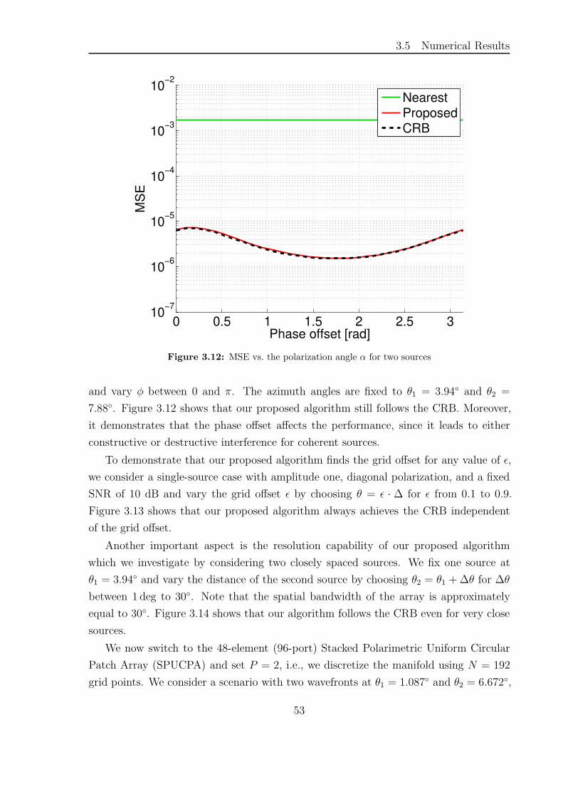
3.5 Numerical Results
0 0.5 1 1.5 2 2.5 310
−7
10−6
10−5
10−4
10−3
10−2
Phase offset [rad]
MS
E
NearestProposedCRB
Figure 3.12: MSE vs. the polarization angle α for two sources
and vary φ between 0 and π. The azimuth angles are fixed to θ1 = 3.94 and θ2 =
7.88. Figure 3.12 shows that our proposed algorithm still follows the CRB. Moreover,
it demonstrates that the phase offset affects the performance, since it leads to either
constructive or destructive interference for coherent sources.
To demonstrate that our proposed algorithm finds the grid offset for any value of ǫ,
we consider a single-source case with amplitude one, diagonal polarization, and a fixed
SNR of 10 dB and vary the grid offset ǫ by choosing θ = ǫ · ∆ for ǫ from 0.1 to 0.9.
Figure 3.13 shows that our proposed algorithm always achieves the CRB independent
of the grid offset.
Another important aspect is the resolution capability of our proposed algorithm
which we investigate by considering two closely spaced sources. We fix one source at
θ1 = 3.94 and vary the distance of the second source by choosing θ2 = θ1 +∆θ for ∆θ
between 1 deg to 30. Note that the spatial bandwidth of the array is approximately
equal to 30. Figure 3.14 shows that our algorithm follows the CRB even for very close
sources.
We now switch to the 48-element (96-port) Stacked Polarimetric Uniform Circular
Patch Array (SPUCPA) and set P = 2, i.e., we discretize the manifold using N = 192
grid points. We consider a scenario with two wavefronts at θ1 = 1.087 and θ2 = 6.672,
53

Chapter 3 Compressive Sensing Based DOA Estimation off the Grid
0.2 0.4 0.6 0.810
−7
10−6
10−5
10−4
10−3
10−2
Grid offset ε
MS
E
NearestProposedCRB
Figure 3.13: MSE vs. the grid offset ǫ for one source
5 10 15 20
10−4
10−3
10−2
Angular separation [deg]
MS
E
ProposedCRB
Figure 3.14: MSE vs. the angular separation for two sources
54

3.6 Summary
−10 0 10 20 30 40 5010
−6
10−4
10−2
100
SNR [dB]
MS
E
NearestProposedCRB
Figure 3.15: MSE vs. the SNR for two sources for the SPUCPA
both diagonally polarized (p1 = p2 = [1, 1]T/√2). The amplitudes are chosen according
to s1 = 1 and s2 = j. Again, the grid offsets are given by ǫ1 = 0.3 and ǫ2 = 0.7. The
MSE vs. the SNR = σ−2n is shown in Figure 3.15. Our proposed algorithm attains the
CRB in the high SNR regime.
3.6 Summary
In this chapter, we address the problem of CS-based DOA estimation for off-grid sources.
We study the spectrum in the case of off-grid sources qualitatively and find that most of
the energy of the off-grid source after reconstruction is concentrated in the two neighbor-
ing grid points. Based on this observation, we derive the best two-term approximation
coefficients explicitly and show that the approximation error is very small for N > M .
Moreover, based on the asymptotically linear behavior of the coefficients with the
grid offset, we propose a very simple scheme to estimate the grid offset based on the
observed coefficients. For multiple sources, we show that this simple scheme still works
well when they are sufficiently spaced. For closely spaced sources, we propose a numerical
procedure for the joint estimation of their offsets from the recovered spectra at their
neighboring grid points. Numerical simulations demonstrate the effectiveness of the
proposed schemes.
55

Chapter 3 Compressive Sensing Based DOA Estimation off the Grid
We show that the CS-based formulation of the DOA estimation problem can be ex-
tended to the polarimetric model, which gives rise to an amplitude vector that possesses
a structured sparsity (with non-zero blocks of size ×1 for each source). We discuss the
off-grid problem in the polarimetric setting and propose an estimator for the grid offset
of one source (or an isolated source) as well as a joint estimator for the grid offsets of
two closely-spaced sources. We show that its cost function can be efficiently calculated
based on the EADF, leading to an overall low computational complexity. Numerical
results demonstrate that the estimators can recover the DOA regardless of the polar-
ization state of the incoming wave and is applicable to arbitrary arrays. Moreover, it
is capable of resolving even very closely-spaced sources and it achieves the Cramer-Rao
Bound.
56

Chapter 4
Compressive Antenna Arrays for
Direction of Arrival Estimation
This chapter deals with the analysis and design of compressive arrays for DOA estima-
tion. Section 4.1 motivates the concept of compressive array and reviews the state of the
art. In Section 4.2 we present a basic receiver architecture for compressive arrays and
introduce a generic system model that includes different options for the hardware imple-
mentation. Based on the generic system model, Section 4.3 deals with the design of the
combining matrix, with the goal to obtain an array that is suitable for DOA estimation.
In Section 4.4, we extend the design approach and propose a design methodology that
focuses the array towards a specific area of interest. The optimized design approaches
proposed are all in 1D DOA estimation (i.e., azimuth). Section 4.5 provides an analysis
of the achievable performance of the proposed compressive arrays for DOA estimation
based on two estimation quality measures: the achievable estimation accuracy, and the
resolution capabilities. Section 4.6 evaluates the proposed approaches via numerical
simulations followed by a summary in Section 4.7.
4.1 Motivation
In general, DOA estimation addresses the problem of locating sources which are radi-
ating energy that is received by an array of sensors with known spatial positions [28].
A major goal in research on DOA estimation is to develop approaches that allow min-
imizing hardware complexity in terms of receiver costs and power consumption while
providing a desired level of estimation accuracy and robustness in the presence of mul-
tiple sources and/or multiple paths. Furthermore, the developed methods shall be ap-
propriate for realistic antenna arrays whose characteristics often significantly vary from
57

Chapter 4 Compressive Antenna Arrays for Direction of Arrival Estimation
commonly considered ideal models [156].
In the last few decades, research on narrow-band DOA estimation using array pro-
cessing has largely focused on uniform arrays (e.g., linear and circular) [28] for which
many efficient parameter estimation algorithms have been developed. Some well-known
examples are ESPRIT [164], MUSIC [137] and Maximum Likelihood (ML)-based meth-
ods [25, 165]. Note that ML-based methods are particularly suitable for realistic, non-
ideal antenna arrays since they can easily account for the full set of parameters of
the antenna array (e.g., antenna polarization, non-ideal antennas and array geometries,
etc.). However, to perform well, the algorithms require to fulfill certain conditions on
the sampling of the wavefront of the incident waves in the spatial domain.
Namely, the distance between adjacent sensors should be less than or equal to half
a wavelength of the impinging planar wavefronts, otherwise it leads to grating lobes
(sidelobes) in the spatial correlation function which correspond to near ambiguities in
the array manifold. At the same time, to achieve DOA estimation with a high resolution,
the receiving arrays should have a relatively large aperture [28]. This implies that arrays
with a large number of antennas are needed to obtain a high resolution, which is not
always feasible.
This limitation has triggered the development of arrays with inter-element spacing
larger than half the impinging wave’s wavelength combined with specific constraints to
control the ambiguity problem in DOA estimation. Such arrays are usually called sparse
arrays. In [166], it was proposed to constitute a non-uniform sparse array with elements
spaced at random positions. However, using such random arrays will often result in
unpredictable behavior of the sidelobes in the array’s spatial correlation function. As a
result, it is necessary to optimize the positions of the antenna elements in order to achieve
a desired performance. An early approach towards that goal was the Minimum Redun-
dancy Linear Array (MRLA) [167], where it is proposed to place the antenna elements
such that the number of pairs of antennas which have the same spatial correlation prop-
erties are as small as possible. However, it is very difficult to construct an MRLA when
the number of elements is relatively large [168]. Some non-linear optimization methods
like genetic algorithms [169] and simulated annealing [170] have been regularly used to
find optimum configurations for these sparse arrays. Moreover, it is shown in [171] that
the optimization of the array aperture with respect to the Cramer-Rao Bound leads to
V-shaped arrays. Recently, it was shown that with co-prime arrays [172], and nested
arrays [173] it is possible to resolve O(N2) of uncorrelated sources with O(N) sensors,
when observed over a large window in time.
Recently, compressive sensing (CS) has been widely suggested for applications that
58

4.1 Motivation
exhibit sparsity in time, frequency or space to reduce the sampling efforts. The usage
of sparse recovery in narrow-band DOA estimation has been considered for applications
like localization of transmitting sources [174], channel modeling [153], tracking and
surveillance in radar [40], and many others. As mentioned earlier in the previous chapter,
if the electromagnetic field is modeled as a superposition of a few plane waves, the DOA
estimation problem can be expressed as a sparse recovery problem. The main focus
there was to use the sparse recovery algorithms that became popular in the CS field
for the DOA estimation problem as an alternative to existing parameter estimation
algorithms [151, 175–177].
Compressed sensing has also been suggested to be applied in the spatial domain
(e.g., array processing and radar) with the main goal to reduce the complexity of the
measurement process by using fewer RF chains and storing less measured data without
the loss of any significant information. Hence, the idea of sparse random arrays with
increased aperture size has been revisited recently and proposed to perform spatial
compressed sensing [178–181].
An alternative approach that attempts to apply CS to the acquisition of the RF
signals that are used for DOA estimation has recently been proposed in [45, 150]. In
particular, the CS paradigm can be applied in the spatial domain by employing N
antenna elements that are combined using an analog combining network to obtain a
smaller number ofM < N receiver channels. Since onlyM channels need to be sampled
and digitized, the hardware complexity1 remains comparably low (e.g., consuming less
energy and storing less data) while a larger aperture is covered which yields a better
selectivity than a traditional, Nyquist (λ/2) spaced M-channel antenna array.
Note that equipping every antenna with an RF chain may imply a prohibitive hard-
ware complexity (in terms of cost as well as power consumption) in certain applications
where reconfigurable arrays with a high gain call for hundreds [182] or even several
thousands of antenna elements [183]. Moreover, using a tunable analog combining net-
work, CS-arrays allow to reconfigure the array on the fly without any change in receiver
hardware. This advantage in flexibility can be crucial in many applications. A recent
example is millimeter wave radio, where one of the major challenges is to solve the gain-
resolution dilemma. In order to account for the high pass loss, a high gain is needed
while at the same time the full angular domain needs to be scanned [184]. A similar
1The hardware complexity (as well as the power consumption) depends on the frequency range, sam-pling rate/bandwidth, array application, exact realization of the antenna array and its elements, real-ization of the phase-shifter network, used RF amplifiers and ADC/DAC components, TX/RX switches,filters, etc. As an exact quantization of the hardware cost savings depends on so many factors and ourapproach is applicable to a wide range of scenarios, we avoid to give concrete numbers in this work.
59

Chapter 4 Compressive Antenna Arrays for Direction of Arrival Estimation
problem occurs during the target acquisition and high resolution target tracking phases
in radar [185]. Because of its flexibility, the compressive hardware architecture is partic-
ularly suitable for these applications (see for example [186] for more precise details on
the practical implementation of such architectures).
In baseband, the operation of the combining network can be described by complex
weights applied to the antenna outputs with a subsequent combination of the received
signals from the antennas. The combining (measurement) matrix that contains the
complex weights and the antenna array form an effective “compressive” array whose
properties define the DOA estimation performance.
In the field of “CS-DOA” it is usually advocated to draw the coefficients of the
measurement matrix from a random distribution (e.g., Gaussian, Bernoulli) [45, 150].
Random matrices have certain guarantees for signal recovery in the noise-free case and
provide some stability guarantees in the noisy case [66,67,187]. However, since no crite-
rion is used to design them, it is likely that they provide sub-optimal performance [4].
In this chapter, we discuss the design and the performance of compressive arrays
employing linear combinations in the analog domain by means of a network of power
splitters, phase shifters, and power combiners. We present a basic receiver architecture
of such a compressive array and introduce a generic system model that includes different
options for the hardware implementation. Importantly, the model reflects the implica-
tions for the noise sources.
Particularly, a well-known source of the receiver noise is the low noise amplifier
(LNA) that is usually placed at the antenna outputs to account for the power losses of
the following distribution/combining network. Depending on the frequency range, the
components of the analog combining network (power combiners, power splitters, phase
shifters) will induce additional losses which also have to be compensated by the LNAs.
To name an example, some typical commercially available phase shifters for phased
array radar applications can induce insertion losses between 5 to 10 dB depending on
the frequency range [188] while architectures based on waveguides promise a loss as low
as 3 dB [183]. This motivates the need for the signal amplification prior to the combining
network.
60

4.1 Motivation
Based on the generic system model we then discuss the design of the combining
matrix, with the goal to obtain an array that is suitable for DOA estimation (i.e.,
minimum variance of DoA estimates and robustness in terms of low side lobe levels or
low probability of false detections). We consider two design approaches. The first is
based on the spatial correlation function which is a low-complexity scheme that in certain
cases even admits a closed-form solution. The second is based on the minimization of the
Cramer-Rao Bound (CRB). Our numerical simulations demonstrate that both proposed
design approaches have a significant performance improvement compared to the state of
the art, namely an array with a randomly chosen combining matrix and a sparse array
with optimized sensor positions.
Furthermore, the compressive array is not only superior to the random and sparse
arrays with respect to its estimation capabilities but also in terms of its ability to alter its
weights on demand and thus facilitate signal-adaptive measurements. The comparison
between the proposed designs demonstrates a trade-off between the minimization of the
CRB and the increase in the sidelobe level. In the proposed design, the trade-off “CRB
vs. sidelobe level” can be controlled by varying the parameters during the optimization.
This provides an additional degree of freedom for the system design that is unavailable
in case of random and sparse arrays.
It is worth mentioning that similar efforts in spatial domain processing exist in the
context of beam space array processing [189–196] and hybrid beamforming [197–199].
In contrast to the element space processing, where signals derived from each element
are weighted and summed to produce the array output, the beam space processing is
a two-stage scheme. The first stage takes the array signals as an input and produces
a set of multiple outputs, which are then weighted and combined to form the array
output. These multiple outputs may be thought of as the output of multiple beams.
The weights applied to different beam outputs are finally optimized according to a
specific optimization criterion [200].
In hybrid beamforming, the main idea is to apply beamforming techniques in both,
the analog and the digital domain [201]. This technique has attracted significant research
attention in millimeter wave (mmWave) applications [202] for the next-generation indoor
and mobile wireless networks [22, 203].
While the overall goal in these areas is similar (reducing the number of digitally pro-
cessed receiver channels), the actual design criterion for the antenna is entirely different
from the one we consider in this work. We aim to obtain an array that is ideally suited
for DOA estimation in the sense that it achieves an accurate estimate (by minimizing
the CRB) while controlling the sidelobe characteristics.
61

Chapter 4 Compressive Antenna Arrays for Direction of Arrival Estimation
4.2 Compressive Arrays
Consider K narrowband plane waves impinging on an array of N antenna elements. At
the antenna output, the received (baseband) signal can be expressed as
y(t) =K∑
k=1
a(γk) · sk(t) + n(t), (4.1)
where y(t) ∈ CN×1 is a vector of antenna outputs, n(t) ∈ CN×1 is an additive noise
vector, t indicates the continuous time, and a(γ) denotes the antenna response as a
function of the parameter vector γ with γT = [θ, ψ,pT] where θ and ψ are the azimuth
and elevation angles and p ∈ C2×1 represents the Jones vector that describes the po-
larization state of the incident plain wave at the receiver. Additionally, sk(t) in (4.1)
denotes the amplitude of the kth source, whereas γTk = [θk, ψk,p
Tk ] is the vector con-
taining its azimuth (θk) and elevation (ψk) angles of arrival along with its Jones vector
pTk = [pk,1, pk,2]. Similar to the previous chapter, it is often useful to write (4.1) in a
matrix form as
y(t) = A · s(t) + n(t). (4.2)
Here, A = [a(γ1),a(γ2), · · · ,a(γK)] ∈ CN×K is the array steering matrix and s(t) =
[s1(t), s2(t), · · · , sK(t)]T ∈ CK×1 is a vector containing the complex amplitudes of the
K sources.
The model in (4.2) presumes a dedicated radio frequency (RF) receiver chain for
each individual antenna element including a low-noise amplifier (LNA), filters, down-
conversion, analog-to-digital (ADC) conversion, etc. For specific applications, however,
such separate RF chains for each antenna element may come at a high cost in terms of
the overall receiver complexity, the amount of data to be processed in the digital domain
(e.g., FPGA) and power consumption.
To further illustrate our point, we show an example from [186] with some realistic
design parameters for a phased antenna array for aeronautical applications at Ka-band
(Rx-direction) in Table 4.1. Considering a typical array gain of 40 to 45 dBi, the
number of required elements of the array is larger than 20,000. Considering the practical
implementation of the RF chain including the low noise amplifier and ADC associated
with each antenna element and all the baseband connections, it turns out that a fully
digital realization of the beamforming network for such an array would not be possible.
In order to reduce the hardware complexity, analog or hybrid combining/beamforming
networks like the one we investigate here are typically considered for such arrays.
62

4.2 Compressive Arrays
Antenna Size 0.75 m (edge size of squared phased array)
Frequency 19.7 GHz (Ka band)
Antenna Efficiency 0.7
Antenna Elements 21609 (assuming λ/2 spacing)
Element gain 2.5 dB (per radiating element, e.g., patch) (assuming λ/2 spacing)
Antenna Gain 44.3 dBi (as a function of effective area)
Table 4.1: Realistic design parameters for a phased antenna array for aeronautical applicationsat Ka-band [186].
In order to reduce the number of RF channels without a loss in the array aperture, we
apply the compressive approach, where the antenna outputs are first linearly combined
in the analog domain and then passed through a lower number of RF chains to obtain
the digital baseband signals as illustrated in Figure 4.1. In this way, M RF receiver
channels (fewer than the N antenna elements) are used for signal processing in the
digital domain. Such a compressive architecture allows reconfiguring the array on the
fly without any change in the receiver hardware which can be very advantageous in
many applications.
The signal combining can be done at different stages within the receiver, e.g., on
the RF (Radio Frequency) signal or at the IF (Intermediate Frequency) stage. The
particular choice on where to place the combining network highly depends on the appli-
cation, especially the considered frequency. In any case, additional signal losses will be
introduced by the power splitters and combiners as well as the phase shifters inside the
combining network. The actual losses’ value will depend on multiple parameters includ-
ing frequency, bandwidth and adaptability of the phase shifters. However, these losses
need to be compensated by LNAs placed in each receiver chain as shown in Figure 4.1.
To this end, let Φ ∈ CM×N denote the analog combining matrix of a compressive
array which compresses the output of N antenna elements to M active RF channels.
Then, the complex (baseband) antenna output (4.2) after combining can be expressed
as
y(t) = Φ (A · s(t) + v(t)) +w(t), (4.3)
where [Φ]m,n = αm,neϕm,n, αm,n ∈ [0, 1], ϕm,n ∈ [0, 2π], m = 1, 2, · · ·M,n = 1, 2, · · · , N ,
whereas v(t) ∈ CN×1 and w(t) ∈ CM×1 are noise vectors with covariance matrices Rvv
and Rww that represent additive noise sources which act before and after the combining
network, respectively.
63

Chapter 4 Compressive Antenna Arrays for Direction of Arrival Estimation
For example, LNAs placed ahead the combining network contribute to v(t) (sig-
nal noise), whereas the ones placed behind the combining network contribute to w(t)
(measurement noise).
Figure 4.1: Compressive array hardware architecture [8]
Let A = Φ · A be the effective array steering matrix after combining, then (4.3)
becomes
y(t) = A · s(t) + n(t), (4.4)
where
n(t) = Φ · v(t) +w(t) (4.5)
is the effective noise vector with covariance Rnn = ΦRvvΦH + Rww. Assuming that
v(t) and w(t) are white with elements that have variance σ21 and σ2
2, respectively, the
covariance of n(t) becomes Rnn = σ21ΦΦH + σ2
2IM . Finally, we define the input SNR as
ρ =Ps
E ‖Rnn‖22=
Ps
σ21‖ΦΦH‖F +Mσ2
2
, (4.6)
where Ps = E ‖s(t)‖22 and ‖ · ‖F denotes the Frobenius norm.
Given (4.4), we aim to design Φ in a way that allows for robust and efficient esti-
mation of the DOAs of the K sources sk(t) from the set of measurements y(t). Hence,
our main design goal includes the minimization of the number of the receiver chains
while providing a minimum variance of the DOA estimates and a reduced probability
of spurious and/or ghost path estimates (i.e., lower sidelobes in the spatial correlation
function).
64

4.3 Design of the Combining Matrix
4.3 Design of the Combining Matrix
4.3.1 Generic Design Approach
Consider the receiver architecture from Figure 4.1 where the combining network is re-
alized by: (i) splitting the analog RF signal of each of the N antennas into L ≤ M
branches; (ii) applying phase shifts in each of the branches; (iii) adding the branches to
form each of theM outputs, which are then passed to theM RF chains. Mathematically,
we model this structure by a matrix Φ with elements given by
[Φ]m,n =
1√L· η · eϕm,n if (m,n) are connected
0 otherwise,(4.7)
where the connections between antennas and ports are such that Φ has L nonzero
elements per column. In (4.7), the factor 1√L
represents the power splitting of each
antenna’s signal to L branches and η ∈ (0, 1] is a scalar parameter that attributes for
the fact that each analog branch (consisting of a power splitter, a phase shifter, and
a combiner) is non-ideal and incorporates losses. A lossless combining network would
correspond to the special case η = 1.
From (4.7), the combining matrix Φ has MN elements that provide MN degrees
of freedom for its design. In the CS literature, a typical approach for choosing Φ
would be to draw ϕm,n randomly. This, however, only gives little control over the array
characteristics. Furthermore, it might result in unwanted effects as high sidelobes and
blind spots [4].
Here, we aim at a design of Φ that results in an effective array that has desired
properties depending on the application scenario, e.g., uniform sensitivity and low cross-
correlation for direction finding, adaptive spatial selectivity for parameter estimation
during beam tracking, etc. Generally, the design task can be formulated as the following
constrained optimization problem
Φopt = argminΦ
J(Φ) s.t. c(Φ, α, β, · · · ), (4.8)
where J(Φ) is some objective function defined by the scenario and c(Φ, α, β, · · · ) rep-
resents the set of optimization constraints. In the following, we propose two particular
formulations of (4.8) for direction finding applications: based on the spatial correlation
function (SCF) and the Cramer-Rao Lower Bound (CRB).
65

Chapter 4 Compressive Antenna Arrays for Direction of Arrival Estimation
For the SCF-based approach, we build our design on the spatial correlation function
defined as
ργ(γ1,γ2) = a(γ1)H · a(γ2), (4.9)
where a(γ) = Φ · a(γ) represents the effective array manifold after combining. The
main idea is to design Φ such that the spatial correlation function ργ(γ1,γ2) follows as
close as possible some pre-specified target T (γ1,γ2). By defining an appropriate target
function, we can provide the desired properties in the spatial correlation function as
discussed in the following.
We then compare the SCF based approach to another optimization approach that is
based on the specific requirements on the estimation accuracy. More specifically, it aims
at improving the accuracy of DOA estimation by designing Φ such that it minimizes the
CRB while keeping the probability of detecting a false direction at a certain (desired)
level.
4.3.2 Design Based on the SCF
For the sake of simplicity, we start by assuming that the sources are located in the
azimuthal plane of the antenna array. Furthermore, the impinging waves are co-polarized
with the antenna array which is assumed to have perfectly matched antennas. Hence,
the effective array manifold depends on the azimuth angle θ only, i.e., a(γ1) = a(θ1).
Under these assumptions, an ideal generic array for direction finding would satisfy
the conditions
ργ(θ1, θ2) = a(θ1)H · a(θ2) =
const θ1 = θ2
0 θ1 6= θ2. (4.10)
The first condition guarantees that the array gain is constant over all azimuth angles
and makes the array uniformly sensitive, whereas the second condition forces optimal
cross-correlation properties to tell signals from different directions apart. However, this
is an example for a generic direction finder. For particular applications, the design goal
may differ, i.e., constraining on a certain sector of angles only or allowing certain values
for the residual cross-correlation. We denote the target function as T (θ1, θ2), where
T (θ1, θ2) = const · δ(θ1 − θ2) represents the ideal generic array (4.10).
Due to the finite aperture of an N -element array, the target in (4.10) can only be
achieved approximately. This allows us to define a criterion for the optimization of Φ
66

4.3 Design of the Combining Matrix
according to the cost function
e(Φ, θ1, θ2) =∣∣a(θ1)
H · a(θ2)− T (θ1, θ2)∣∣ (4.11)
=∣∣a(θ1)
H ·ΦH ·Φ · a(θ2)− T (θ1, θ2)∣∣ .
We can approximate the continuous variables θ1 and θ2 by considering the P -point
sampling grid θ(G)p , p = 1, 2, . . . , P and define the P ×P matrices E and T according to
E(i,j) = e(Φ, θ(G)i , θ
(G)j ) and T(i,j) = T (θ
(G)i , θ
(G)j ). Note that since the array manifolds
are smooth functions, it is sufficient to choose the sampling grid slightly above Nyquist,
i.e., P = c ·N where c > 1. We typically choose c between 2 and 4 in our experiments.
After insertion into (4.11), we obtain
E =∣∣AH ·ΦH ·Φ ·A− T
∣∣ . (4.12)
Based on (4.12), the quality of Φ can be assessed by a suitable norm of E. As a first
step, let us consider the Frobenius norm, i.e., we optimize Φ according to
Φopt = argminΦ
‖E‖2F . (4.13)
In the special case2 where A ·AH = C · IN , with C being a constant, the optimization
problem in (4.13) admits a closed-form solution as shown in the following theorem.
Theorem 1. Let S = A·T ·AH and let SM be a rank-M-truncated version of S obtained
by setting its P −M smallest eigenvalues to zero. Then the set of optimal solutions to
(4.13) is given by the set of matrices Φ that satisfy ΦHΦ = SM .
Proof. To prove the theorem, we use the fact that for a unitary matrix U and an
arbitrary square matrix X we have ‖X ·U‖F = ‖U ·X‖F = ‖X‖F . Since A satisfies
A·AH = N ·IM we can find a matrix A ∈ C(M−N)×N such that V.= 1/
√N ·[AT, AT]T ∈
CN×N is a unitary matrix. Therefore, we have V ·AH =[√
N · IM , 0M×N−M
]T
.
2This condition is, e.g., fulfilled for an ULA if the sampling grid is chosen to be uniform in the spatialfrequencies (direction cosines). Moreover, for many arrays the condition is approximately fulfilled (e.g.,for UCAs). In this case, the closed-form solution can still be applied as a heuristic method.
67

Chapter 4 Compressive Antenna Arrays for Direction of Arrival Estimation
The cost function (4.13) can then be rewritten as
‖E‖2F =∥∥V ·E · V H
∥∥2
F
=
∥∥∥∥∥∥
√NIM
0N−M×M
ΦHΦ[√
NIM , 0M×N−M
]
− V TV H
∥∥∥∥∥∥
2
F
=
∥∥∥∥∥∥
NΦH ·Φ 0M×N−M
0N−M×M 0N−M×N−M
−N ·
A
A
T[
AH, AH
]
∥∥∥∥∥∥
2
F
=
∥∥∥∥∥∥
N ·
ΦH ·Φ−A · T ·AH −A · T · AH
−A · T ·AH −A · T · AH
∥∥∥∥∥∥
2
F
= N2 ·∥∥ΦH ·Φ− S
∥∥2
F+ const, (4.14)
using the short-hand notation S = A · T ·AH. Equation (4.14) demonstrates that the
optimization problem is equivalent to finding the best approximation of the matrix S by
the matrix ΦH ·Φ. Since Φ is an m×M matrix, the rank of the M ×M matrix ΦH ·Φis less than or equal to m < M . Therefore, (4.14) represents a low-rank approximation
problem. According to the Eckart-Young theorem, its optimal solution is given by
truncating the M −m smallest eigenvalues of S.
In other words, Theorem 1 states that we can find an optimal Φ by computing a
square-root factor of the best rank-M approximation of S. Moreover, the following
corollary can be found from Theorem 1:
Corollary 1. Under the conditions of Theorem 1, any matrix Φ is optimal in terms
of the “ideal” target from (4.10) if and only if the rows of Φ have equal norm and are
mutually orthogonal.
Proof. The sampled version of (4.10) is given by a scaled identity matrix, i.e., T = C ·IN .Since A is row-orthogonal, it follows that S = A ·T ·AH = C ·N ·IM . As all eigenvalues
of S are equal to C · N , its eigenvalue decomposition can be written as S = U · (C ·N · IM) ·UH, where U ∈ CM×M is an arbitrary unitary matrix. Truncating the M −m
“smallest” eigenvalues, we obtain Sm = C · N · Um · UHm, where Um ∈ CM×m contains
the first m columns of U . Invoking Theorem 1, we have ΦHoptΦopt = C · N · Um · UH
m
and therefore Φopt is a scaled version of UHm, which proves the claim.
Corollary 1 agrees with the intuition that the measurements (i.e., the rows of Φ)
should be chosen such that they are orthogonal in order to make every observation as
68

4.3 Design of the Combining Matrix
informative as possible. In addition, the corollary shows that this choice also minimizes∥∥ΦHΦ− C · P · IM
∥∥Fwhich contains the correlations between all pairs of columns in Φ
as well as the deviation of the columns’ norms (therefore, in a sense, this choice minimizes
the “average” mutual correlation). On the other hand, this also demonstrates that
the optimization in (4.13) is not sufficiently selective since all row-orthogonal matrices
achieve the same minimum of the cost function.
The cost function (4.13) assigns equal weight to the error for all pairs of grid points
θ(G)1 , θ
(G)2 , i.e., it tries to maintain the resemblance to the target spatial correlation func-
tion T in the mainlobe area with the same weight as in the certain off-diagonal regions
that contain the sidelobes. In practice, however, it is often desirable to have more con-
trol over the shape of the spatial correlation function. There are many ways additional
constraints could be incorporated in the optimization, e.g., maximum constraints on
the magnitude of cross-correlation in some region and interval constraints on the auto-
correlation inside the mainlobe. For numerical tractability, we follow a simpler approach
by introducing a weighting matrix W ∈ RP×P into (4.13). The modified optimization
problem is given by
Φopt = argminΦ
‖E ⊙W ‖2F , (4.15)
where ⊙ represents the Schur (element-wise) product. The weighting matrix allows
to put more or less weight on the main diagonal certain off-diagonal regions, or even
placing zeros for regions that remain arbitrary. Thereby, more flexibility is gained and
the solution can be tuned to more specific requirements.
The drawback of (4.15) is that it does not admit a closed-form solution in general.
However, it can be solved by numerical optimization routines that are available in mod-
ern technical computing languages.
4.3.3 Design Based on the CRB
For the case of a single source, a correlation-based DOA estimator amounts to find the
DOA that corresponds to the global maximum in the beamformer spectrum D(θ)
D(θ) = |aH(θ)y(t)|2, (4.16)
with a(θ) ≡ Φ · a(θ). Note that in this case, (4.16) is equivalent to the maximum
likelihood (ML) cost function, and therefore, the correlation-based DOA estimator is
equivalent to the ML estimator. We define then the false detection as the event where
69

Chapter 4 Compressive Antenna Arrays for Direction of Arrival Estimation
the global maximum in the beamformer spectrum D(θ) is outside the mainlobe area
(either 3-dB or null-to-null beamwidth). The error probability Pd is hence given by
Pd ≡ Prob(∃θ ∈ U : D(θ0) < D(θ)
), (4.17)
where U denotes the set of DOAs corresponding to the directions in the beamformer
spectrum outside the mainlobe area while θ0 /∈ U is the true DOA that corresponds to
the mainlobe peak.
A direct evaluation of (4.17) is analytically intractable. In [204], an analytic expres-
sion for the false detection probability has been derived and given as
Pd ≤1
2G
L∑
q=1
G∑
g=1
Ψq
(
(2g − 1)π
2G
)
(4.18)
The analytic expression for the false detection probability can now be used to opti-
mize the combining matrix Φ with the objective to improve the CRB while keeping the
probability of false detection below some desired level ǫ0 for a given input SNR ρ0.
This said, for detection of a single source, we can formulate it as
Φopt =argminΦ
maxθ0
CRB(Φ, θ0) (4.19)
s. t. Pd(Φ, θ0, ρ0) < ǫ0.
To derive CRB(Φ, θ0), we use the expression in [28] for the receiver model shown
in Figure 4.1 where the noise vectors v(t) and w(t) are assumed to be white with
covariances Rvv = σ21IN and Rww = σ2
2IM , respectively. The associated CRB matrix is
then found to be
CRB(Φ, θ) = σ21
(2Re
F ⊙RT
s
)−1, (4.20)
where ⊙ denotes Schur (element-wise) matrix product, Rs = s(t)sH(t) is the signal
covariance matrix, and F is a matrix that depends on the array beam pattern and the
combining matrix Φ as
F = DHΦHZΦD. (4.21)
Substituting in (4.21),
Z = Q(
IN − A(
AHQA)−1
AHQ)
,
D =[∂a(θ0)/∂θ0, ∂a(θ1)/∂θ1, ..., ∂a(θK−1)/∂θK−1
],
70

4.4 Adaptive Focusing Design
and Q = (ΦΦH + βIN)−1 where β =
σ22
σ21. Since we consider only a single source
for solving the optimization problem in (4.19), F reduces to a scalar F and Rs to
Rss = ‖s(t)‖2. Therefore, for a single source (4.20) becomes
CRB(Φ, θ0) = σ21
(
2FRss
)−1
=1
2Fζ, (4.22)
where ζ = Rss
σ21is the input SNR.
Both the constraint and the objective in (4.19) are non-convex functions with respect
to (Φ, θ0). The optimization problem is thereby a non-convex problem exhibiting a
multi-modal cost function, where the optimal (global) solution can only be found by an
exhaustive search strategy. Therefore, we apply a local minimizer to the above problem
using an algorithm based on the interior-reflective Newton method [205], [206]. However,
by using this algorithm the obtained solution strongly depends on the initialization of
the parameters (Φ, θ0). Moreover, there is no guarantee that the global optimum is
found.
One way of addressing this issue is to apply the algorithm several times, where for
each run the initialization of the parameters (Φ, θ0) is different. In doing so, the obtained
solution to (4.19) is likely to be sufficiently close to the optimal solution. However, it
might be time consuming due to the complexity of the optimization problem at hand.
Another way of tackling this problem is to first obtain a solution for Φ by the SCF
approach described above and then use it for the initialization in (4.19).
So far, we have discussed the case of a single source’s wave impinging on the antenna
array. However, we can easily extend the CRB design approach to account for the
presence of multiple signal sources by applying the full CRB given by (4.20) in (4.19) and
modifying the false detection probability expression in (4.18). Particularly, assuming a
correlation-based DOA estimator, we need to compute the false detection probability of
the strongest source being falsely detected in the presence of K − 1 weaker ones (see [8]
for more details).
4.4 Adaptive Focusing Design
In (4.8), our target is a static combining matrix that yields an array with certain prop-
erties, such as uniform sensitivity and low sidelobe level, which is a good choice if no
prior knowledge of the targeted sources is available. However, we can extend this ap-
proach towards an adaptive design that makes use of the fact that for a slowly changing
scene, the estimates from the previous snapshots provide prior information about the
71

Chapter 4 Compressive Antenna Arrays for Direction of Arrival Estimation
source locations in the next snapshots. This fact can be utilized for adaptive focusing
of the array’s sensitivity towards regions of interest where the targets are expected [7].
In doing so, the SNR and the effective resolution in these directions of interest can
be further improved, resulting in a superior DOA estimation performance. To achieve
this, we adopt a sequential measurement strategy which starts with a combining matrix
designed for uniform sensitivity and then gradually refine it towards the directions of
interest that have been identified in the observations collected so far [7].
The main idea is to design Φ such that the spatial correlation function r(θ1, θ2).=
a(θ1)H · a(θ2) follows as close as possible to a prespecified target T (θ1, θ2), i.e., a matrix
Φ that minimizes
e(Φ, θ1, θ2) = |r(θ1, θ2)− T (θ1, θ2)| (4.23)
The target T (θ1, θ2) is adapted to the current knowledge of the scene. A uniform target
function is used when no prior knowledge is available. When regions of interest have been
specified (e.g., via an estimate of the angular power spectrum or a previous reconstructed
scene), the target can be adapted to focus on these regions in order to provide a superior
estimate (e.g., improved SNR and/or resolution).
To this end, an ideal uniform target function can be described by
Tuni(θ1, θ2) =
const θ1 = θ2
0 θ1 6= θ2, (4.24)
where the first condition guarantees that the array gain is constant for all angles (to
make the array uniformly sensitive in all directions) and the second condition asks for
good cross-correlation properties to tell signals from different directions apart.
On the other hand, a target function that focuses in an interval Θ is given by
TΘ(θ1, θ2) =
const θ1 = θ2 ∈ Θ
0 θ1 6= θ2, (4.25)
where the interval Θ can for instance be describe by a center cθ and a width wθ via
Θ =[cθ − wθ
2, cθ +
wθ
2
].
In order to find a matrix Φ that minimizes (4.23), we utilize the mechanism intro-
duced earlier in Section 4.3.2 which we restate here for convenience. It is based on the
following steps: First, to eliminate the continuous variables θ1 and θ2, we consider the
N -point sampling grid θ(G)n , n = 1, 2, . . . , N used for CS and define the N ×N matrices
72

4.4 Adaptive Focusing Design
R and T according to R(i,j) = r(θ(G)i , θ
(G)j ) and T(i,j) = T (θ
(G)i , θ
(G)j ). Note that R
can be written as R = AH · ΦH · Φ · A. The deviation between the sampled spatial
correlation function R and its target T can then be measured via a suitable norm of
the error matrix E.= R−T . A closed-form solution for Φ can be obtained if we choose
the Frobenius norm of E. In particular, if we let
Φopt = argminΦ
‖E‖2F . (4.26)
we can obtain Φopt via the following procedure: Let S = A · T ·AH and let Sm be a
rank-m-truncated version of S obtained by setting its N − m smallest eigenvalues to
zero. Then every square-root factor of Sm (i.e., any Φ satisfying ΦHΦ = Sm) is an
optimal solution to (4.26) [4].
Since Φopt can be obtained in closed form with a very low computational complexity,
it is feasible to adapt it during the observations, i.e., the target can be refined to the
current knowledge of the scene.
The adaptation mechanism proceeds as follows:
1. We begin by scanning the scene with a matrix Φ designed according to (4.13) or
(4.15), designed for a uniform target T or according to (4.19) for the full angular
range θ0 ∈ (0, 2π].
2. Identify regions of interest based on an estimate of the angular power spectrum
obtained from the initial observation(s).
3. Define a focusing region Θ as the union of all regions of interest.
4. Modify Φ by solving (4.26) for a target designed for the focusing region Θ in the
SCF-based approach or solving (4.19) with a restricted angular range.
5. As the sources are assumed to change their position gradually, track sources by
repeating steps (2) to (4) sequentially, moving the regions of interest along with
the currently identified source locations.
6. Every S snapshots, rescan the scene with a matrix Φ designed for a uniform
sensitivity in order to detect newly appearing sources. If new sources are found,
incorporate their location into the set Θ.
The parameter S represents a design parameter that determines how quickly the system
reacts to sources appearing outside the current direction of interest.
73

Chapter 4 Compressive Antenna Arrays for Direction of Arrival Estimation
4.5 Estimation Quality
In this section, we provide an analysis of the achievable performance of the proposed
compressive arrays for DOA estimation. In the noisy case, there are two main estimation
quality measures: the achievable estimation accuracy, and the resolution capabilities.
Estimation Accuracy
For a fixed aperture, the achievable accuracy is mainly determined by the effective SNR
at the antenna output. For this reason, we compare the SNR of a compressive array
and a sparse array3 at the same number of active channels M .
We express the output signal for a single source via (4.3) as
y(t) = Φ · a(γ1) · s1(t) + n(t), (4.27)
where the elements of Φ are given by (4.7) and the covariance of n(t) is given by
Rnn = σ21ΦΦH + σ2
2IM . The SNR of the compressed array can then be computed as
ρc =E‖Φ · a(γ1) · s1(t)‖2
trace Rnn
=‖Φ · a(γ1)‖2 · Ps
trace ΦHΦσ21 +Mσ2
2
=trace
Φ · a(γ1) · aH(γ1) ·ΦH
· Ps
trace ΦHΦσ21 +Mσ2
2
, (4.28)
where Ps = E |s1(t)|2 is the source power.
As evident from (4.28), the SNR is dependent on the parameter vector γ, i.e., on the
DOA. It is therefore meaningful to consider the average SNR over all possible source
directions. This requires to compute the average of g(γ) = ‖Φ · a(γ)‖2 over γ which
is not possible without further assumptions either about the array or about Φ. Let g
be the average of g(γ) over γ, i.e., g = Γ−1∫g(γ)dγ with Γ =
∫1dγ. Moreover, let us
define the matrix J = Γ−1∫a(γ) ·a(γ)Hdγ so that g = trace
Φ · J ·ΦH
. To proceed,
we would like to replace g by traceΦΦH
. We can always do so when J = IN which
implies that the beam patterns of all antennas are orthogonal over the entire parameter
space. This is, e.g., fulfilled for an ULA if it is parametrized by spatial frequencies
3By sparse arrays we mean here any array that is capable of providing a larger aperture than a“traditional” array with λ/2-spaced elements, while having a dedicated receiver channel for each antennaelement. Examples of sparse arrays include arrays with randomly positioned elements [178–181] as wellas nested and co-prime arrays [172, 173].
74

4.5 Estimation Quality
µ = cos(θ). Furthermore, for J 6= IN one can show that EΦ g = EΦ
trace
ΦΦH
for any random ensemble of Φ where its elements are i.i.d. Note that in our case, due
to (4.7), traceΦΦH
is not random but deterministic. Hence, the expectation on the
right-hand side is not needed. In light of this assumption, we can express the average
SNR ρc (averaged over γ) as
ρc =trace
ΦΦH
· Ps
trace ΦHΦ σ21 +Mσ2
2
=‖Φ‖2F · Ps
‖Φ‖2F σ21 +Mσ2
2
(4.29)
Using (4.7) it is easy to see that ‖Φ‖2F =(
η√L
)2
·N ·L = η2 ·N . Therefore, the average
SNR becomes
ρc =η2 ·N · Ps
η2 ·Nσ21 +Mσ2
2
=PS
σ22
· η2 ·Nη2 ·N · σ2
1
σ22+M
(4.30)
To compare this SNR to the one that can be achieved with a sparse array we model
the observed signal as as(γ1) · s1(t) +ws(t), where the elements of ws(t) are i.i.d. with
variance σ22 .
We then obtain for the SNR of a sparse array
ρs =M · Ps
Mσ22
=Ps
σ22
. (4.31)
Therefore, the ratio of the SNRs becomes
ρcρs
=η2 ·N
η2 ·N · σ21
σ22+M
(4.32)
Overall, this shows that if there is significant signal noise (i.e., σ21 ≫ σ2
2) in the com-
pressed arrays, their achieved SNR degrades linearly with the ratio of signal to mea-
surement noise power compared to sparse arrays. On the other hand, for dominating
measurement noise (i.e., σ21 ≪ σ2
2), the SNR ratio approaches η2 NM
which means an SNR
improvement if the efficiency of the lossy components satisfies η >√
MN. In practice,
the compression ratio NM
can be quite high and therefore, the SNR improvement of the
compressive arrays can be very significant.
Note that another particular advantage of the proposed compressive arrays is their
reconfigurability, as discussed in Section 4.4. If we follow this idea, the array performs
beamforming towards the already detected targets. In this case, the SNR is further
improved by the beamforming gain which is a factor on the order of N .
75

Chapter 4 Compressive Antenna Arrays for Direction of Arrival Estimation
Resolution
The ability to distinguish closely spaced sources is an important characteristic of an
antenna array. The achievable resolution of the array mainly depends on its aperture,
i.e., the largest distance between pairs of antenna elements. For ULAs, the aperture is
equal to (N−1)λ/2 since the elements are spaced in half-wavelength distance from each
other. For compressive arrays as well as sparse arrays, this distance can be increased
further. As a result, the array’s correlation function becomes sharper, at the price
of an increase in sidelobes (grating lobes). We can control the height of the grating
lobes by proper design of the antenna placement (in the case of sparse arrays) as well
as the analog combining network (in the case of compressive arrays). In general, we
expect that at the same covered aperture and the same number of active RF chains, the
compressive arrays will have lower sidelobes (since the many degrees of freedom in the
analog combining network allow to suppress the sidelobes significantly). As it is difficult
to quantify the achievable sidelobe suppression analytically, we will focus on this aspect
in the numerical results in Section 4.6.
4.6 Numerical Results
In this section, we evaluate the performance of the compressive array with an optimized
combining network and compare it to its closest counterparts in terms of the aperture
and hardware complexity, namely random and sparse arrays. We also evaluate the
performance of the adaptive focusing design showing its advantages over the uniform
one.
4.6.1 Performance Analysis of the SCF Based Design
We start first by examining the SCF- based design. To this end, we consider an M =
12 element ULA that is reduced to m = 8, 6, 4 channels via an m × 12 combining
matrix Φ. This matrix is chosen according to [Φ](m,n) = eϕm,n , where ϕm,n are the
optimization variables in the proposed approach and drawn from a uniform distribution
for the random approach.
It is certainly possible to include the amplitude in the design process as well. Of
course, this requires additional analog components, since in addition to phase shifters
we will also need attenuators to adjust the amplitudes. These do not only increase
the complexity of the combining network but also introduce additional losses and noise.
For this reason, it is very common to consider only phase shifters in these networks,
76

4.6 Numerical Results
which already provide a lot of flexibility. This is one of the baseline assumptions in the
mmWave hybrid beamforming community (see e.g., [203] and references therein) and in
SatCom applications (see e.g., [184]).
Figure 4.2: SCF-approach: phase-only optimization (left) vs. optimization of amplitude andphase (right) for two different weight matrices.
Nevertheless, to give an example of performance loses due to considering the phase
only instead of amplitudes and phases we have conducted an experiment which is shown
in Figure 4.2. Here we compare the SCF-based optimization forM = 12, m = 8, P = 48,
using the SCF of the uncompressed 12-ULA as a target T . The weight matrix is chosen
such that it is equal to one for the mean beam (i.e., four points to the left and the right
of the main diagonal) and w for all other points, such that higher values of w put more
emphasis on the side lobes. For w = 0.1 (top two plots) and w = 0.5 (bottom two
plots), we compare optimizing only the phase of Φ (left) with optimizing magnitude
and phase of Φ) (right). Each graph displays the mean of the average SCF (solid blue
line) as well as the 10/90 percentiles (shaded area) over 1000 random initializations of
the SCF-based optimization method. We observe that for w = 0.1 there is barely any
77

Chapter 4 Compressive Antenna Arrays for Direction of Arrival Estimation
visible change, whereas for w = 0.5 the side lobes are suppressed slightly stronger, at
the expense of a reduction of the main lobe peak. In general, the difference between
optimizing only phase or magnitude and phase is not very pronounced since satisfactory
results can be already achieved by optimizing the phase.
To find an optimized design Φopt, we solve the weighted optimization problem (4.15)
via Matlab’s numerical optimization features. We run fmincon with 100 random
initializations and pick the solution with the smallest value of the cost function. As a
target we set T = AH ·A which is the correlation function we would achieve with anM-
ULA. The weighting matrix is chosen according to [W ](n1,n2) = ρ|n1−n2| where ρ ∈ (0, 1]
is a parameter that controls the decay of the weights. Essentially, smaller values of ρ
put significantly more weight at the main lobe and its quick decay and less weight on
the side-lobes that are far from the main lobe. The limiting value ρ = 1 represents the
unweighted case.
Figure 4.3 demonstrates the advantage of using a measurement matrix Φ that is
optimized according to our proposed methodology as compared to choosing Φ randomly.
The SCF of the random design (Figure 4.3a) suffers many blind spots and high side lobes
whereas the optimized design enjoys a smooth main lobe and relatively low side lobe
level.
0 0.2 0.4 0.6 0.8 1
Spatial frequency [2 rad]
0
0.2
0.4
0.6
0.8
1
Sp
atia
l fr
eq
ue
ncy [
2 r
ad
]
(a) Random
0 0.2 0.4 0.6 0.8 1
Spatial frequency [2 rad]
0
0.2
0.4
0.6
0.8
1
Sp
atia
l fr
eq
ue
ncy [
2 r
ad
]
(b) Optimized SCF
Figure 4.3: SCF comparison for an SCF optimized design versus random ones for M = 12 andm = 8.
Figure 4.4 depicts the normalized spatial correlation function (SCF) defined as
ϕ(µ1, µ1 +∆µ) =a(µ1)
Ha(µ1 +∆µ)
a(µ1)Ha(µ1)(4.33)
for µ1 = π. For reference, the black line indicates the 12-ULA whereas the blue line
78

4.6 Numerical Results
represents the result of the optimization for ρ = 0.95. We observe that the optimized
design comes close to the M-ULA except for slightly higher sidelobes. Figure 4.4 also
shows the SCFs that are obtained when we draw Φ randomly without any optimization.
We depict the average SCF (solid line), the 5-th and the 95-th percentile (shaded area)
and one example realization (dash-dotted line). As evident from the figure, randomly
chosen measurement matrices lead to significantly higher spatial correlations. In partic-
ular, every realization shows sidelobes that are sometimes even higher than the main
lobe.
PSfrag replacements
Figure 4.4: Spatial correlation function ϕ(µ1, µ1 + ∆µ) for µ1 = π. We compare the M = 12element ULA with an 8× 12 CS array. To show the variability of choosing Φ randomly, we depictthe average correlation (solid line), the 5-th and 95-th percentile (shaded area) and one examplerealization (dash-dotted line).
Figure 4.5 demonstrates the DOA estimation performance if we use the OMP algo-
rithm for the sparse recovery stage. We consider a noise-free scenario with two sources
that are located on the N = 48 point uniform sampling grid, i.e., µ1,2 = (n0 ± d/2) ·∆where n0 ∈ [1, N ] and d is the inter-source spacing in grid points. For each value of
d, the mean square error MSE = 12
∑2k=1(µk − µk)
2 is averaged over all values of n0.
An estimate of the Complementary Cumulative Distribution Function (CCDF) of this
average MSE obtained from 1000 realizations of Φ is shown. As evident from the figure,
the average MSE exceeds the source spacing d with a probability of 95 % for d = 2, 80 %
for d = 4, and 30 % for d = 8. For the same scenario, our optimized design (choosing
w = 0.7) achieves an MSE very close to zero (shown with the dashed lines), i.e., 0.72∆
for d = 2, 0.13∆ for d = 4, and 0.03∆ for d = 8.
79

Chapter 4 Compressive Antenna Arrays for Direction of Arrival Estimation
0 5 10 150
0.2
0.4
0.6
0.8
1
Average MSE in units of ∆
CC
DF
Random, d = 2Random, d = 4Random, d = 8Optim., d = 2Optim., d = 4Optim., d = 8
Figure 4.5: Mean square estimation error for randomly drawn Φ, using OMP for the sparserecovery step. We consider two sources positioned at µ1,2 = (n0 ± d/2) ·∆. The MSE is averagedover all values n0 ∈ [1, N ] and a histogram over this average MSE is estimated for three values ofthe source distance d = 2, 4, 8. MSE and source distance are shown in units of the grid spacing∆ to facilitate their comparison. The average MSE of our optimized design is indicated with thedashed lines.
0 5 10 150
0.2
0.4
0.6
0.8
1
Average MSE in units of ∆
CC
DF
Random, d = 2Random, d = 4Random, d = 8Optim., d = 2Optim., d = 4Optim., d = 8
Figure 4.6: The same scenario as shown in Figure 4.5 but this time including noise at an SNRof 10 dB.
80

4.6 Numerical Results
To investigate the effect of additive noise, we have repeated the experiment from Fig-
ure 4.5 with additive noise. In particular, we have drawn the noise vector w (cf. (5.12))
from a zero mean circularly symmetric complex Gaussian distribution with a variance
of 0.1, which corresponds to an SNR of 10 dB. The result is shown in Figure 4.6. Once
more, the optimized design achieves a significantly lower average MSE compared to the
randomly chosen measurement matrices.
Though the main concern for optimizing Φ has been put on correlation-based re-
covery algorithms such as the OMP, we have tested it on the Basis Pursuit (BP) algo-
rithm [97] as well and found that it also offers some advantages there. To this end, we
have repeated the previous simulation with the same parameters, using BP instead of
OMP for the recovery stage. The result is shown in Figure 4.7. The figure shows the
CCDF of the average MSE over 1000 random realizations of Φ. Our proposed design
is not shown since it achieves an exact reconstruction result (MSE=0) for all values of
d. As expected, BP is more reliable and less sensitive to sidelobes compared to OMP.
In fact, for each value of d there is a non-zero chance to draw a matrix Φ randomly
that achieves an exact reconstruction as well. However, these “lucky” choices are not
very stable in the sense that changing the grid size N or the source spacing d results in
estimation errors to occur.
10−2
10−1
100
0
0.2
0.4
0.6
0.8
1
Average MSE in units of ∆
CC
DF
Random, d = 2Random, d = 4Random, d = 8
Figure 4.7: The same scenario as shown in Figure 4.5, this time using Basis Pursuit (BP) for therecovery stage. Our proposed design achieves an average MSE of zero for d = 2, 4, and 8.
81

Chapter 4 Compressive Antenna Arrays for Direction of Arrival Estimation
4.6.2 Comparison to the CRB Based Design and Sparse
Arrays
We now compare the SCF based design to the CRB based one and also to sparse arrays.
The latter can be obtained by varying the element positions of a “traditional” antenna
array to achieve a high resolution (low CRB). Via a careful design of the element po-
sitions, the level of the resulting grating lobes can be controlled (cf., e.g., [171]). Note
that we do not compare our design to nested or co-prime arrays [172,173]. While these
approaches in theory allow to construct O(M2) virtual sensors from O(M) antennas,
this is only possible if we observe the scene over a large number of snapshots in time
(during which it must remain static) and all sources are mutually uncorrelated. Since
the proposed array as well as optimized sparse arrays can operate on an arbitrary num-
ber of snapshots (down to the single snapshot case) and have no restrictions in terms
of the source correlation, a comparison of the achievable accuracy and resolution with
nested or co-prime arrays would not be fair.
We change our scenario to reduce the optimization complexity for the CRB based
design and use UCAs instead of ULAs. We perform the numerical study based on a
uniform circular array (UCA) with N = 9 elements that are compressed to M = 5
receiver channels (this amounts to ≈ 1.8 times reduction in the number of receiver
channels). Note that for a UCA with isotropic elements the response of the nth antenna
element as a function of the azimuth angle θ can be written as
an(θ) = e2πR cos(θ−ϑn), (4.34)
where ϑn = 2π(n−1)/N with n = 1, 2, · · · , N and R = Rλis the array radius normalized
to the wavelength. For both proposed designs, the radius R was fixed and set to 0.65.
The combining matrix Φ is chosen according to [Φ](m,n) = eϕm,n , where ϕm,n are
the optimization variables in the proposed approaches. This implies that the role of
the efficiency η is not considered, implicitly assuming η = 1. Note that this is not
uncommon in the related literature [203, 207]. Moreover, for η < 1, the sidelobe level
(and thus the false detection probability) are unaffected while the CRB scales linearly
with η2. Therefore, for low values of η, sparse arrays may outperform the proposed
compressive arrays. On the other hand, the latter are reconfigurable and can hence
perform beamforming in the directions of interest, to partially compensate the analog
combining losses.
To find an optimized design Φopt, we solve the weighted optimization problems (4.15)
and (4.19) via Matlab’s numerical optimization features. Since run-time is not a
82

4.6 Numerical Results
concern for an off-line design, and in order to avoid local minima, we run fmincon and
fminimax to solve (4.15) and (4.19), respectively, with 100 random initializations and
pick the solution with the smallest value of the cost function. In the following, we
refer to the design obtained by the SCF optimization approach from (4.15) as Opt SCF,
whereas the design obtained as a result of the CRB minimization from (4.19) is referred
to as Opt CRB. For the Opt SCF approach, we set T = AH · A as a target which
is the correlation function we would achieve with an M-element (uncompressed) UCA.
The weighting matrix is chosen according to [W ](n1,n2) = w|n1−n2| where w ∈ (0, 1] is a
parameter that controls the decay of the weights. Essentially, smaller values of w put
significantly more weight at the main lobe and its quick decay and less weight on the
side-lobes that are far from the main lobe. The limiting value w = 1 represents the
unweighted case. For the Opt CRB approach, the threshold false detection probability
ǫ0 is set to 0.05 to be achieved at an input SNR of ρ0 = 0dB.
We begin by examining the performance of the optimized compressive arrays with
respect to the attainable CRB and the sidelobe level in the case of a single source as
discussed in Sections 4.3.2 and 4.3.3.
CRB [rad2]0.08 0.09 0.1 0.11 0.12 0.13 0.14 0.15
CCDF
0
0.1
0.2
0.3
0.4
0.5
0.6
0.7
0.8
0.9
1
RandomOpt SCFOpt CRB
Figure 4.8: Comparison of the CRBs of the optimized compressive arrays versus the randomones. The CCDF of the CRB for 5000 random realizations are shown together with that of theoptimized kernel.
Figure 4.8 shows the achievable CRB of the compressive arrays with the optimized
combining network and the random ones that have the same number of antennas and
sampling channels while ϕm,n are drawn uniformly at random from (0, 2π]. At a fixed
83

Chapter 4 Compressive Antenna Arrays for Direction of Arrival Estimation
SNR level of 0 dB, an estimate of the Complementary Cumulative Distribution Function
(CCDF) of the CRB obtained from 5000 random realizations of Φ is shown. The opti-
mized networks for both approaches have been designed to achieve the same CRB. This
has been done by varying w of the Opt SCF approach such that the resulting optimized
Φ achieves a similar CRB as the one obtained from the Opt CRB approach. As evident
from the figure, the CRB of the optimized compressive arrays is almost in every case
lower than that of the random ones. In other words, the random kernel can potentially
provide a performance comparable to the optimized ones but with a very low probability.
The CCDFs of the average sidelobe levels for the same scenario are shown in Figure 4.9.
We observe that the random compressive arrays provide significantly higher sidelobe lev-
els compared to both the SCF and the CRB-optimized ones. This supports the intuition
that designing the combining matrix randomly results in sub-optimal performance.
Sidelobe Level0.55 0.6 0.65 0.7 0.75 0.8 0.85 0.9
CCDF
0
0.1
0.2
0.3
0.4
0.5
0.6
0.7
0.8
0.9
1
RandomOpt SCFOpt CRB
Figure 4.9: Comparison of the sidelobe levels of the optimized linear combining network versusthe random ones. The CCDF of the mean sidelobe levels for 5000 random realizations are showntogether with that of the optimized kernel.
Comparing the sidelobe level of the SCF and CRB-optimized compressive arrays, we
can notice that the latter has a lower sidelobe level at a specific CRB. This is confirmed
by the corresponding (analytic) probabilities of false detection depicted in Figure 4.10.
For comparison Figure 4.10 also presents the results for the uncompressed UCAs with
N = 9 and N = 5 (i.e., with smaller aperture size) as well as the average Pd for the
random arrays. As can be seen, both proposed approaches achieve lower probability
of false detection Pd than the uncompressed UCA with a lower number of antennas,
84

4.6 Numerical Results
whereas the sparse arrays on average are significantly inferior to all the rest. It is worth
noting that for both proposed optimization approaches, the CRB and the sidelobe level
(and hence the probability of false detection) can be controlled: explicitly in the case of
the CRB-based approach via setting a threshold ǫ0 on Pd, and indirectly in the case of
the SCF-based approach via a proper choice of the weighting matrix W in (4.15).
SNR [dB]-4 -2 0 2 4 6 8 10 12 14
Pd
10-4
10-3
10-2
10-1
100
RandUCA N = 5Opt SCFOpt CRBUCA N = 9Threshold
Figure 4.10: False detection probability of the uncompressed UCAs, compressive arrays, and therandom ones.
Now we compare the compressive array to a sparse array that has the same number
of receiver chains, i.e., for the considered scenario it means that for a sparse array
N =M = 5. According to [171], we design the sparse array such that the positions of its
elements are optimized towards obtaining a uniform sensitivity and desired CRB. Note
that this results in an array geometry closely resembling that of a V-shaped array [171].
Figure 4.11 shows the spatial correlation functions at a specific DOA for the sparse array
and an SCF-optimized compressive array (compression from N = 9 elements to M = 5
receiver chains) that achieves the same CRB (0.113) at the fixed SNR level of 0 dB. It
can be noted that the sidelobe level of the sparse array is relatively high compared to
that of the compressive one (especially the Opt CRB design). Particularly, the mean
level of the sidelobes for the optimized compressive array is 0.53 compared to 0.68 of
the sparse array.
85

Chapter 4 Compressive Antenna Arrays for Direction of Arrival Estimation
Azimuth DOA θ [rad]0 1 2 3 4 5 6
SpatialCorrelationFunction
0
0.1
0.2
0.3
0.4
0.5
0.6
0.7
0.8
0.9
1
SparseOpt SCFOpt CRB
Figure 4.11: The spatial correlation function at a specific DOA of an optimized sparse array anda compressive array with the same number of receiver chains and an optimized combining network
CRB [rad2]0.08 0.085 0.09 0.095 0.1 0.105 0.11 0.115 0.12
Sidelob
eLevel
0.45
0.5
0.55
0.6
0.65
0.7
SparseOpt SCFOpt CRB
Figure 4.12: The CRB versus the sidelobe level for a compressive array with an optimizedcombining network and a sparse array (single diamond marker)
Figure 4.12 shows the resulting trade-off between providing a good CRB and main-
taining a low sidelobe level. One can see that the compressive array (with either of the
optimization schemes) outperforms the sparse one and gives more degrees of freedom
86

4.6 Numerical Results
to tune the array design with respect to some desired properties (e.g., targeted CRB
or sidelobe level). This figure also confirms once again that the Opt CRB approach
outperforms the Opt SCF approach as it gives more control over the sidelobe level for a
specific CRB. Note that the comparison to the sparse array is optimistic since it assumes
an efficiency of η = 1. For η < 1, the sidelobe level is unaffected but the CRB scales
linearly with η2, shifting the Opt SCF and Opt CRB curves to the right. However, one
should not forget that in contrast to the sparse array, the proposed arrays are reconfig-
urable, allowing to carry out beamforming in directions of interest once some targets
have been detected. This beamforming can partially compensate the analog combining
losses.
The superiority of the compressive arrays over the sparse ones with respect to adapt-
ability is further highlighted in Figure 4.13. It presents the CRB and the sidelobe level
of an optimized compressive array as a function of the number of antennas N . It is clear
that the compressive arrays not only allow to control the CRB and the sidelobe level via
an optimization of the combining network, but also by adding more antenna elements
while the number of receiver channels is kept fixed. In Figure 4.13, we can see that the
CRB can be improved significantly when the number of antenna elements is increased
at the price of higher sidelobe levels. However the network can then be re-optimized for
the new scenario (e.g., with the Opt CRB approach), aiming at a better suppression of
the sidelobes while a certain level of CRB improvement is maintained.
Number of Antennas (N)
5 10 15 20 25 30
CR
B
0
0.05
0.1
0.15
0.2
0.25S
idel
ob
e L
evel
0.5
0.6
0.7
0.8
0.9
1
CRBSidelobe Level
0.5
0.6
0.7
0.8
0.9
1
Figure 4.13: The CRB and the sidelobe level for a compressive array with different number ofantenna elements and fixed number of channels
87

Chapter 4 Compressive Antenna Arrays for Direction of Arrival Estimation
Now we examine the performance of the proposed optimized compressive array in
the case of two sources impinging on the array from different DOAs. The power ratio
between the two sources is set to α = |s2/s1|2 = −6 dB, while their DOAs are d radians
apart, i.e., θ1 = θ, θ2 = θ + d where θ scans the whole angular space. The two sources
are inphase.
CRB [rad2]0 0.1 0.2 0.3 0.4 0.5 0.6 0.7 0.8 0.9 1
CCDF
0
0.1
0.2
0.3
0.4
0.5
0.6
0.7
0.8
0.9
1
Random, d = 0.2 [rad]Opt SCF, d = 0.2 [rad]Random, d = 0.4 [rad]Opt SCF, d = 0.4 [rad]
Figure 4.14: Comparison of the CRBs of the optimized compressive arrays versus the randomones for the case of two impinging sources. The CCDF of the CRB for 5000 random realizationsare shown together with that of the optimized kernel.
Similar to Figure 4.8, Figure 4.14 shows the achievable CRB of the strongest path
using the compressive arrays with the optimized combining network and the random
ones that have the same number of antennas and sampling channels for an SNR level
(with respect to the strongest source) of 12 dB. The CCDF of the CRB obtained from
5000 random realizations of Φ is shown for d = 0.2 and d = 0.4 radians. As discussed
earlier, the Opt SCF and the Opt CRB designs both provide the same CRB and so only
the Opt SCF is shown for clarity. The CCDF shows that the CRB of the optimized
compressive arrays is again almost in every case lower than that of the random ones.
As the sources get closer (e.g., d = 0.2), the need for the optimized network increases as
the probability to achieve acceptable properties (e.g., low CRB) by the random design
gets lower.
88

4.6 Numerical Results
SNR [dB]0 2 4 6 8 10 12 14 16 18 20
Pd
10-4
10-3
10-2
10-1
100
RandUCA N = 5Opt SCFOpt CRBUCA N = 9Threshold
Figure 4.15: False detection probability of the uncompressed UCAs, compressive arrays, and therandom ones with two source signals with power ratio α = −6dB.
It has been proposed in Section 4.3.3, to extend the design based on CRB for the
case of multiple sources. Considering the same set-up with two sources, and for a
specific DOA of the first source, to do so the sidelobes in the correlation function have
to be searched for all possible DOAs of the second source. This leads to a very high
computational complexity. The same search strategy has to be performed for all possible
DOAs of the first source. Therefore, for simplicity, we fix the second source DOA and
perform the optimization similar to that of the single source case. Figure 4.15 shows the
probabilities of false detection Pd for two sources. It can be seen that the design based on
CRB shows superior performance in terms of lower false detection probability compared
to that of the uncompressed (N = 5)-element UCA, compressive array with SCF based
designed network, and the averaged random ones. Although the SCF based design can
not be re-optimized for the multiple source case, it still provides a significantly lower
probability of false detection compared to the random arrays and is comparable to a
non-compressed (N = 5)-element UCA.
4.6.3 Performance Analysis for Adaptive Focusing
In this section, we present some numerical results to demonstrate the advantage of using
the focusing measurement matrix design according to our proposed methodology. To
this end, we consider a M = 12 element ULA that is reduced to m = 8 channels via an
89

Chapter 4 Compressive Antenna Arrays for Direction of Arrival Estimation
8 × 12 compression/focusing matrix Φ. We sample the spatial space using an N = 64
point uniform sampling grid, i.e., µ1,2 = (n0 ± d/2) · ∆ where n0 ∈ [1, N ] and d is the
inter-source spacing in grid points.
To construct the uniform matrix ensemble Φuni we solve the optimization prob-
lem (4.26) to obtain the closed form solution. As a target we set Tuni = IN which is
the ideal uniform target function described by (4.24). We will only consider it here as
an initial estimator of the regions of interest towards which the main beam is focused
afterwards.
PSfrag replacements
w
c
dθ
1
TargetT(θ, θ)
w∆ w∆
Figure 4.16: Definition of the focusing window: the blue arrows indicate the estimated DOAswith a distance of d grid points. The window is centered at grid point c, located in the middle ofthe targets, and has a width of w grid points, where w = d+ 2w∆.
The focusing measurement design Φfoc is obtained by modifying the target according
to (4.25) where Tfocus is an N × N matrix that contains the identity matrix in the
focusing region and nulls otherwise. The focusing region is identified based on an initial
estimate of the source locations, e.g., by a reconstruction of the scene based on a first
measurement carried out with Φuni. Figure 4.16 shows how to define the target for two
closely spaced sources, in which case we define one interval containing both as the region
of interest. The blue arrows represent the (estimated) source positions. The focusing
interval Θ is described as mentioned earlier by a center grid point c which we place in
the middle of the two sources and a width w. Naturally, we have w = d + 2w∆, where
w∆ is the number of extra grid points we allow to both sides of the identified sources (in
Figure 4.16 we have w∆ = 1) and d is the distance between the sources estimated from
the uniform measurement initialization step. In general, the width w represents a design
parameter where smaller values indicate a more narrow focus. If the initial estimate of
the regions of interest is not very reliable, w should be chosen larger to allow for some
90

4.6 Numerical Results
deviations of the source position estimate in the refocused measurements. A concrete
strategy for the choice of w is discussed below. Note that if more than two sources are
present, the focusing interval Θ can be found by the union of several intervals, each
centered around the middle of a cluster of identified sources.
As a first step, we compare the performances of the three measurement designs of Φ:
the random design advocated in the earlier papers [45, 150], the uniform we proposed
in [4] and the focusing design proposed in this work. The latter uses the estimate of the
uniform design as an initialization, i.e., its first measurement is carried out with Φuni,
the scene is reconstructed, and then used to identify the regions of interest to find Φfoc
for the second measurement. For this experiment, we choose w∆ = 6, i.e., a window
width of w = d+ 12 grid points as the focusing region.
0 5 10 15 20 25
10−1
100
SNR [dB]
MS
E [ra
d]
Rand
Uniform
Focused
Figure 4.17: MSE versus SNR for two sources using the random, uniform, and focusing designwhere the source separation d is varied randomly. The focusing interval is defined according tothe knowledge about the region of interest obtained from the first uniform measurement with awindow width given by w∆ = 6.
Figure 4.17 shows the mean square error (MSE) versus the signal to noise ratio (SNR)
for a scenario with two sources that are located on the grid and d grid points apart.
The MSE is averaged over randomly drawn distances d and noise vectors w (cf. (5.12))
drawn from a zero mean circularly symmetric complex Gaussian distribution. For each
trial, the fast orthogonal matching pursuit (OMP) [106] is used for the DOA estimation
process and then the mean square error MSE = 12
∑2k=1(µk − µk)
2 is calculated for the
three designs.
91

Chapter 4 Compressive Antenna Arrays for Direction of Arrival Estimation
As depicted in the figure, the random measurement design shows the worst perfor-
mance as expected (see [4] for more details). The results show that the focusing design
provides a significant improvement in terms of the SNR.
To investigate the effect of the focusing interval width, we have repeated the exper-
iment from Figure 4.17 with different focusing widths while fixing the sources’ spacing
to d = 4 which corresponds to 0.75 Rayleigh distances (i.e., they are closely spaced).
Figure 4.18 compares the resulting MSE for a focusing width parameter w∆ = 3, 5,
and 7, respectively. We observe that a more narrow focus leads to significantly reduced
MSEs and thus a superior resolution of the two closely spaced sources compared to the
unfocused, uniform design.
−5 0 5 10 15 2010
−2
10−1
100
SNR [dB]
MS
E [ra
d]
w∆ = 7
w∆ = 5
w∆ = 3
Uniform
Figure 4.18: MSE versus SNR for two sources separated by four grid points using differentfocusing interval lengths. A smaller window size leads to a more narrow focus, resulting in animproved resolution.
We now turn our attention towards a concrete example of a possible implementation
of our focusing design without any special prior knowledge about the scene. Our idea
is to perform the focusing sequentially, starting with an unfocused, uniform design and
then gradually narrowing the focus by sequentially reducing the window size w. Each
of the sequential measurements provides an improved estimate of the scene (as we have
seen in Figure 4.18) which can be used to update the center of the window c and thus
make sure that the focus is put in the correct direction.
92

4.6 Numerical Results
−5 0 5 10 15 2010
−2
10−1
100
SNR [dB]
MS
E [ra
d]
w∆ 1 = N/2
w∆ 2 = N/4
w∆ 3 = N/8
w∆ 4 = N/16
Uniform
Figure 4.19: Same scenario as shown in Figure 4.18 but this time the focusing is done sequentiallywith w∆ being halved at each step.
−5 0 5 10 15 2010
−1
100
SNR [dB]
MS
E [ra
d]
w∆ 1 = N/2
w∆ 2 = N/4
w∆ 3 = N/8
w∆ 4 = N/16
Uniform
Figure 4.20: Same scenario as shown in Figure 4.19 but this time the sources are only d = 2 gridintervals apart.
Figure 4.19 shows such a process where we investigate a scenario with two sources
d = 4 grid points apart and we keep decreasing the window size parameter w∆ from N/2
93

Chapter 4 Compressive Antenna Arrays for Direction of Arrival Estimation
to N/4 to N/8 to N/16. The curves labeled w∆,i for i = 1, 2, 3, 4 correspond to the i-th
sequential measurement which positions the target window according to the estimate
from the (i− 1)-th measurement and sets the window size to N/2i, as indicated in the
legend of the figure. The results show that each of the sequential measurements provides
a more narrow focus which leads to a lower MSE, although the change from N/8 to N/16
does not improve the MSE significantly anymore.
Figure 4.20 depicts the result for the same scenario with the sources only d = 2 grid
points apart. Here the fourth measurement w∆,i = N/16 shows a worse performance
than the third measurement using w∆,3 = N/8. This suggests that over-focusing might
result in a worse performance, e.g., if the focus center c is not placed exactly in the
correct direction.
So far, all the numerical results were based on the OMP algorithm for the sparse
recovery step. To demonstrate that our proposed measurement matrix design can be
applied to any sparse recovery algorithm, Figure 4.21 shows the same scenario as Fig-
ure 4.18, comparing the basis pursuit (BP) [97] with the OMP algorithm. The results
show that as expected, the convex optimization based BP algorithm outperforms OMP,
however, both algorithms benefit in a similar way from our proposed adaptive measure-
ment matrix design.
−5 0 5 10 15 2010
−2
10−1
100
101
SNR [dB]
MS
E [ra
d]
BP Uniform
OMP Uniform
BP Focusing
OMP Focusing
Figure 4.21: Same scenario as before but instead using BP for initialization
94

4.7 Summary
4.7 Summary
In this chapter we consider the design of compressive antenna arrays for direction of
arrival (DOA) that aim to provide a larger aperture with a reduced hardware complex-
ity and allowing reconfigurability compared to traditional array designs. We present an
architecture of such a compressive array and introduce a generic system model that in-
cludes different options for the hardware implementation. We then focus on the choice of
the coefficients in the analog combining network. We have demonstrated that choosing
it randomly may lead to undesirable effects in the effective CS array such as very high
sidelobes. These are particularly problematic for correlation-based sparse recovery algo-
rithms such as the Orthogonal Matching Pursuit since they may lead to the detection
of spurious peaks.
Instead of choosing them randomly, we propose a generic design approach for the
analog combining network with the goal to obtain an array with certain desired proper-
ties, e.g., uniform sensitivity, low cross-correlation, or low variance in the DOA estimates.
We exemplify the array design via two concrete examples. Our numerical simulations
demonstrate the superiority of the proposed optimized compressive arrays to compres-
sive arrays with randomly chosen combining kernels, as the latter result in very high
sidelobes (which imply a higher probability of false detection) as well as higher CRBs.
We also compare our optimized compressive array to a sparse array of the same com-
plexity (i.e., same number of receiver channels M) and find that sparse arrays suffer
from much higher sidelobes at the same CRB level. Also our proposed compressive
array enjoys a high degree of adaptability since the combining weights can be altered to
adjust the array to the current requirements, which is impossible for sparse arrays due
to their static nature.
We have also proposed a focusing design of the compression matrix based on the SCF
technique. The main idea is to apply measurements in a sequential fashion: first, we
measure with a uniform design that is equally sensitive in all directions and thus allows
us to obtain a good estimate for the region(s) of interest in the angular domain. Then,
the measurements are iteratively focused towards these regions. We have demonstrated
that the focusing design results in a significant performance improvement compared to
the uniform design. In particular, our numerical results demonstrated that a narrower
focus, leads to an improved SNR and resolution. We have demonstrated that the width
of the focusing region is a parameter that can be used to control the degree of focus
depending on the reliability of the estimate of the regions of interest and provided a
sequential focusing strategy as a concrete example.
95

Chapter 4 Compressive Antenna Arrays for Direction of Arrival Estimation
96

Chapter 5
Compressive Time Delay Estimation
This chapter extends the ideas from the previous chapters applying them to time delay es-
timation (TDE) and synchronization. After the motivation in Section 5.1, we introduce
the TDE model in Section 5.2. The compressive sensing (CS) based TDE architecture
is then presented in Section 5.3 followed by a description of the TDE procedure in the
compressed domain in Section 5.4. In Section 5.5 an optimization based design for the
measurement kernels of the CS based TDE architectures is proposed extending the ideas
from the previous chapter. Afterwards, we deal with the synchronization of the TDE
network in Section 5.6 and propose a CS based reference broadcast synchronization
where the reference signal is an opportunistic signal already in the system. Section 5.7
evaluates the proposed approaches via numerical simulations followed by a summary in
Section 5.8.
5.1 Motivation
Time delay estimation (TDE) is a fundamental challenge arising in many applications
such as wireless communications [208], radar [209], localization [210], sensor networks
[211], and many others. A wide range of TDE techniques have been proposed, see,
e.g., [212] for a survey for TDE in linear dynamic systems.
In this chapter, we treat the special case of estimating the delay of a signal with a
known pulse shape from a noisy superposition of several delayed copies. Such problems
occur in synchronization of wireless sensor networks [213], localization [214] or wideband
channel estimation [215] due to the multipath channel.
The complexity bottleneck in these systems is the high data rate from the high-speed
AD converters that are required to sample the wideband signals which are used to ensure
a high resolution in time. However, since the pulse shape is known, the actual rate of
97

Chapter 5 Compressive Time Delay Estimation
(unknown) information in the received signals is low. Therefore, it has been proposed
to apply compressed sensing (CS) to reduce the hardware complexity while maintaining
high precision. In [216,217], a framework for sampling time-delayed signals is presented
based on a union of subspaces approach [218]. The authors derive sufficient conditions
on the transmitted pulse and the sampling functions in order to ensure perfect recovery
of the channel parameters in the absence of noise, which includes conditions on the
minimal required sampling rate.
Considering concrete choices of the low rate sampling kernels, it is often suggested
in the CS literature to use random kernels which are incoherent with any basis and
so achieving informative measurements even at low rates. Though randomly chosen
kernels represent a simple and generic approach, it is known that they do not provide the
optimal robustness against noise. Only recently, the optimization of the measurement
kernels has been investigated [219–221]. In particular, [219] studies the optimization of
a discrete measurement matrix in time domain and [220] consider a continuous (sum-
of-sincs) kernel in time domain whose output that is sampled at a sub-Nyquist rate.
Both use criteria inspired by the Bayesian Cramer-Rao bound to optimize the kernels.
In [221], the measurement matrix is optimized such that for a given (overcomplete) basis,
the sensing matrix has a small average coherence.
In this chapter, we propose another optimization based design for the measurement
kernels of the CS based TDE architectures. We consider an architecture based on a
bank of K continuous-time periodic functionals that are sampled once per period. We
show that their Fourier-domain representation allows to optimize these functions based
on a finite number of coefficients. We demonstrate numerically that the optimized CS
kernels outperform a randomly chosen one in terms of the delay estimation accuracy.
It is also worth mentioning that the fully wireless operation for TDE also poses
significant synchronization challenges compared to a wired network (i.e., precise time
synchronization is essential). A certain degree of synchronization is required in any WSN
in order to establish the communication protocols. However, some TDE applications
such as using a WSN for wireless distributed localization of a set of targets, require a
very accurate synchronization which is even more challenging.
The simplest approach for synchronizing a WSN is given by transmitting a known
reference signal from at least one node in the network. Each node can then obtain
its timing information by comparing the known signal to its own received copy [213].
However, accurate timing information requires a reference signal with high bandwidth,
thus consuming precious resources (when done wirelessly).
A promising alternative approach to the problem is presented in [211, 222] and ex-
98

5.1 Motivation
REF
RX
RX N
Signal of
Opportunity
RX 1
TX 1
TX M
Figure 5.1: Example WSN using signals of opportunity for the wireless synchronization. Theblue nodes represent the WSN that shall localize the green tags.
emplified in Figure 5.1. Using so-called signals of opportunity like communication (e.g.,
LTE) or broadcast (e.g., DVB-T) signals, a precise time synchronization between the RX
nodes can be realized. Since it is desirable that the system is able to use arbitrary signals
of opportunity, it should operate without having to fully decode these signals (which
would be impossible, e.g., for LTE signals). Traditionally, orthogonal frequency division
multiplexing (OFDM) receivers synchronize themselves on the received signal [223–225].
Additionally, the own or the remote clock error may be modeled and corrected accord-
ing to [226]. However, this requires that either the signal is completely demodulated
or even decoded [224, 225] or this requires that small pieces of the received signal at
the reference RX (REF RX) are distributed to all other RX (Figure 5.1, blue arrows)
via a data link. We refer to this as the reference signal. At the RX the received time
sampled copy of the reference signal is compared with the originally received signals of
opportunity (Figure 5.1, red arrow) and a time difference between the local clocks and
the clock of the REF RX can be estimated.
It is clear that retransmitting the wideband reference signal requires significant re-
sources. In [222], it is proposed to extract features from the OFDM symbol stream and
compare the features in a centralized unit for timing offset compensation. In this work,
we propose to compress the reference signal before transmission to all other nodes. We
rely on the basic ideas of CS to design the compression matrix without significantly
affecting the properties of the correlation function which determine the synchroniza-
99

Chapter 5 Compressive Time Delay Estimation
tion precision compared to the original non-compressed scenario. We show that the
correlation can be calculated in the compressed domain, yet achieving correlation char-
acteristics comparable to the high bandwidth correlation obtained with opportunistic
signals. In particular, we demonstrate that the compression does not affect the width of
the main peak in the correlation function, but rather it leads to higher cross-correlation
levels. Therefore, the compression ratio allows to control the trade-off between the
required bandwidth of the reference node and the effective SNR which can be tolerated.
5.2 Time Delay Estimation
The time delay estimation (TDE) between a reference signal and its delayed version is a
fundamental problem arising in many applications such as wireless communications [208],
radar [209], localization [210], sensor networks [211], and many others.
In a typical scenario, a pulse with a priori known shape is transmitted through a
medium. As a result, the received signal is composed of a delayed and a weighted replica
of the transmitted pulse. In various applications, the time delay and the gain coefficient
have to be estimated from the received signal.
A typical TDE problem can be described as:
y(t) = G(p)u(t− Td) + n(t), (5.1)
where the signal u(t) is the so called reference signal, y(t) is the one measured (i.e.,
recieved), n(t) is the measurement noise and G(p) is a linear system (without time-
delay). The time delay to be determined is Td. The signal can be either wideband
or narrowband. They can also be either real valued or complex valued. Complex (or
analytic) signal representation is often used for narrowband signals but can also be used
for wideband signals. The impulse response g(t) of G(p) can also be complex valued.
Complex signals and impulse responses are commonly used for bandpass systems, e.g.,
in radar and communications.
A wide range of TDE techniques have been proposed, see, e.g., [212] for a survey
for TDE in linear dynamic systems. The conventional method of TDE uses the cross-
correlation between the reference and the delayed signal and estimates the time delay
by finding the maximum of this cross-correlation [227, 228].
The time delay estimation problem can be formalized as follows. A transmitter sends
a signal s(t) to allow a receiver (or multiple receivers) that know s(t) to synchronize
themselves. For simplicity, we assume that s(t) is tp-periodic, i.e., s(t) = s(t + tp).
100

5.3 Compressive Sampling TDE Architecture
Periodic synchronization signals are common, e.g., in GNSS [229] and UWB Radar
applications [230]. They allow receivers to keep track of the synchronization over time
and to average over multiple periods. For the problem at hand, another advantage is
that since these signals are also band-limited to a certain bandwidth B, they can be
completely described by a finite number of M = B · tp coefficients. Therefore, we can
write s(t) as
s(t) =∑
m∈Mcs[m]e
2πm ttp (5.2)
where M is the set of points in frequency where s(t) is non-zero1 with |M| =M .
Due to the multipath nature of wireless propagation channels, the receiver observes
a weighted sum of delayed copies of s(t), i.e., the received signal can be written as
x(t) =
L∑
ℓ=1
αℓs(t− τℓ) + w(t), (5.3)
where αℓ and τℓ represent the complex amplitude and delay of the ℓ-th propagation path
for ℓ = 1, 2, . . . , L, respectively, and w(t) is the additive white Gaussian measurement
noise. Note that since s(t) is tp-periodic so is x(t) (besides for the additive noise).
5.3 Compressive Sampling TDE Architecture
We employ a compressive sampling architecture similar to [216], which is depicted in
Figure 5.2. After an initial downconversion stage to remove the carrier frequency2,
instead of sampling the received signal x(t) directly, the receiver performs a bank of
analog multiplications with the functions pk(t), k = 1, 2, . . . , K, followed by sampling
with a lower rate to yield the coefficients ψk. Since x(t) is periodic, it is convenient to
choose pk(t) such that they are also tp-periodic.
1We employ a complex representation of all signals, which can refer to the complex low-pass domainwhere M = −M
2 + 1, . . . , M2 or analytic signals where only the positive half of the spectrum is
considered.2The transmitter sends the bandwidth-B signal by modulating it onto a carrier frequency fc, which
is removed at this stage. The signal model is described entirely in the complex low-pass domain.
101

Chapter 5 Compressive Time Delay Estimation
PSfrag replacements
x(t)xc(t)
fc
p1(t)
p2(t)
pK(t)
ψ1
ψ2
ψK
∫
tp
∫
tp
∫
tp
Figure 5.2: Compressive receiver architecture: the signal is multiplied with K periodic waveformspk(t) and the result is sampled once per period in each branch.
The overall sampling rate of the receiver is then equal to Ktp
= KM
· B which means
that the compression factor relative to Nyquist sampling is equal to KM. Note that each
of the K ADCs operates at a rate BM, i.e., a factorM times lower than in a conventional
system.
It is important to note that since our receiver is linear and x(t) is a linear combination
of delayed copies of s(t), it is sufficient to describe the sampling of one delayed signal
s(t − τ). Once a mathematical model for this has been obtained, the sampled version
of x(t) follows from a trivial linear combination.
Therefore, if we let x(t) = s(t− τ), the k-th sample ψk for k = 1, 2, . . . , K is given
by
ψk(τ) =1
tp
∫
tp
pk(t)∗ · s(t− τ)dt. (5.4)
As both, pk(t) and s(t) are periodic, they can be expressed using a discrete representation
in the Fourier domain, namely
pk(t) =
∞∑
m=−∞cp,k[m]e
2πm ttp . (5.5)
With the help of (5.5) and (5.2), we can now rewrite (5.4) in frequency domain [216].
102

5.3 Compressive Sampling TDE Architecture
For clarity, let us begin with τ = 0 to obtain
ψk(0) =1
tp
∫
tp
( ∞∑
m1=−∞c∗p,k[m1]e
−2πm1ttp
)
·(∑
m2∈Mcs[m2]e
2πm2ttp
)
dt
=∞∑
m1=−∞
∑
m2∈Mc∗p,k[m1]cs[m2]
1
tp
∫
e−2πm1
ttp e
2πm2ttp dt
︸ ︷︷ ︸
tp·δ[m1−m2]
=∑
m∈Mc∗p,k[m]cs[m]. (5.6)
Equation (5.6) shows, not surprisingly, that only the M coefficients of pk(t) that
coincide with the spectral support of s(t) contribute to the coefficients ψk. Therefore, if
the hardware realization allows it, they should be chosen such that they are bandlimited
to B as well3.
Introducing the short hand notations cs ∈ CM×1 and cp,k ∈ CM×1 for the M coeffi-
cients that cs[m] and cp,k[m] in (5.6) we then have ψk(0) = cHp,k · cs. Moreover, it is now
easy to carry out the same computation for τ 6= 0. We obtain
ψk(τ) =∑
m∈Mc∗p,k[m]e
−2πm τtp cs[m]
= cHp,k · diagd(τ) · cs, (5.7)
= cHp,k · diagcs · d(τ), (5.8)
where we have defined the vector d(τ) =[
e−2πm τ
tp
]
m∈M.
Based on (5.8), the entire vector of observations ψ(τ) ∈ CK×1 can be described as
ψ(τ) = [ψ1(τ), . . . , ψK(τ)]T = CH
p · diagcs · d(τ), (5.9)
where Cp = [cp,1, . . . , cp,K] ∈ CM×K contains the coefficients of all the K sequences
pk(t). Equation (5.9) describes the observed output vector for a single delayed copy of
s(t). Since our receiver is linear, the observed vector y ∈ CK×1 for the input signal x(t)
3Compressive sampling architectures that use PN-sequences for the pk(t) have been proposed, e.g.,the modulated wideband converter [216]. Although these are not strictly bandlimited to B, theirpractical advantage is that they can be realized in hardware up to very high switching speeds.
103

Chapter 5 Compressive Time Delay Estimation
according to (5.3) is given by
y =
L∑
ℓ=1
αℓψ(τℓ) + w, (5.10)
where w ∈ CK×1 is the effective noise vector.
5.4 Delay Estimation Procedure
5.4.1 Gridded Sparse Recovery Based Estimator
Equation (5.10) shows that our observation vector can be modeled as a weighted sum of
L terms ψ(τℓ) under additive noise. Since ψ(τ) is known to the receiver, this suggests
that the delays can be recovered from y if L < K. The difficulty in estimating the delays
lies in the fact that they can take any value from a continuous domain. A common and
very simple approach to tackle such problems is to discretize the parameter space into
an N -point sampling grid in τ referred to as τ(G)n , n = 1, 2, . . . , N . In the special case
of a uniform sampling grid, we have τ(G)n = (n− 1) ·∆τ , n = 1, 2, . . . , N where ∆τ = tp
N.
Based on the sampled delays, we can define a basis Ψ ∈ CK×N according to
Ψ =[
ψ(
τ(G)1
)
, ψ(
τ(G)2
)
, . . . , ψ(
τ(G)N
)]
. (5.11)
Since the delays τℓ can take any value, they will not be on any predefined sampling
grid almost surely. However, it has been shown that if the sampling of the grid is not too
coarse, one can still use the fact that y is approximately sparse in Ψ and apply suitable
grid offset estimation procedures to correct for the mismatch between the grid points
and the actual delays, cf. e.g., [231] for a comparison of interpolation strategies in this
setting. Therefore, to facilitate the further explanations we now assume that all the
delays τℓ were exactly on the sampling grid, i.e., τℓ = τ(G)dℓ
for some dℓ ∈ 1, 2, . . . , N.This allows us to write y as
y = Ψ ·α+ w, (5.12)
where α ∈ CN×1 contains αℓ at the indices dℓ for ℓ = 1, 2, . . . , L and zeros otherwise. In
other words, besides for the noise, y is L-sparse in Ψ. The delay estimation problem
104

5.5 Measurement Design
can then be cast as a sparse recovery problem, e.g.,
min ‖α‖1 s.t. ‖y −Ψ ·α‖22 ≤ σ2, (5.13)
where σ2 is an estimate of the noise power. Note that it has been shown in [216] that
K ≥ 2L is sufficient to recover all the delays from y in the noise-free case.
5.4.2 Correlation Based Estimator
A simpler estimator is inspired by traditional, Nyquist-sampling based systems which
simply correlate the observed signal with the known waveform and then estimate the
location of the peak. Note that if there is only one path (L = 1) or if paths are very
well separated (by more than the width of the correlation peak), this method is in fact
optimal. Along these lines, the correlation based estimator in our setting is defined as
τ = argmaxτ
∣∣∣∣
ψ(τ)H · yψ(τ)H ·ψ(τ)
∣∣∣∣, (5.14)
where the peak search is not limited to a prespecified grid. It is instructive to expand
(5.14) for the special case L = 1 where we obtain
τ = argmaxτ
α1 ·ψ(τ)H ·ψ(τ1)ψ(τ)H ·ψ(τ)︸ ︷︷ ︸
ρ(c)(τ)
+ψ(τ)H · wψ(τ)H ·ψ(τ) . (5.15)
Equation (5.15) shows that we are essentially finding the peak in the “compressed”
correlation function ρ(c)(τ).
5.5 Measurement Design
The previous sections have shown how the CS based receiver can be employed for delay
estimation. As we have seen, it provides a sparsifying basis ψ(τ) for the signal and
the atoms ψ(τ) depend on the choice of the signal s(t) (through the vector cs) and the
sampling functions pk(t) (through the matrix Cp). In this section, we shed some light
on their proper choice to obtain a good synchronization performance.
105

Chapter 5 Compressive Time Delay Estimation
An “ideal” choice of ψ(τ) would satisfy the conditions
ψ(τ1)H ·ψ(τ2) ≈
0 τ1 6= τ2
const τ1 = τ2,(5.16)
where the first condition asks for good cross-correlation properties between different
delays and the second condition guarantees that the measurement is equally sensitive
to all possible delays. This choice will ensure that the compressed correlation function
ρ(c)(τ) introduced in (5.15) is close to the ideal delta function. At the same time, it is also
beneficial for the gridded sparse recovery based estimator since the first condition asks
for low correlation between the columns of the sensing matrix Ψ (i.e., a low coherence)
and the second condition guarantees that all columns have similar norms (to achieve a
uniform sensitivity for all possible delays).
To measure how well a given matrix Φ satisfies (5.16), we can formulate an error
measure of the form e(Φ, τ1, τ2) = (ψ(τ1)H ·ψ(τ2)−C ·δ[τ1−τ2])·ωτ1,τ2 where ωτ1,τ2 ∈ R≥0
is a weight function which allows to trade the weight between certain (τ1, τ2) regions,
e.g., between uniform sensitivity (τ1 = τ2) and low cross-correlation (τ1 6= τ2).
However, since it is difficult to minimize the error over the continuous variables τ1
and τ2 we consider it only on the N -point sampling grid introduced earlier. This leads
to an error matrix E(Φ) ∈ RN×N given by
E(Φ) =[e(Φ, τ (G)
n1, τ (G)
n2)]
(n1,n2=1,2,...,N)
=(ΨH ·Ψ− C · IN
)⊙Ω, (5.17)
=(DH · diagc∗s ·Cp ·CH
p · diagcs ·D − C · IN)⊙Ω,
=(DH ·
([Cp ·CH
p
]⊙[c∗s · cTs
])·D − C · IN
)⊙Ω,
where we have used (5.9) to rewrite Ψ and defined D = [d(τ(G)1 ), . . . , d(τ
(G)N )] ∈
CM×N . Moreover, ⊙ in (5.17) denotes the Hadamard-Schur (elementwise) product and
Ω contains the weights ωτ1,τ2 . Based on (5.17), the quality of Ψ can be measured via an
appropriate norm of E. For instance, minimizing the (weighted) average squared error
corresponds to minimizing the squared Frobenius norm of E, whereas minimizing the
maximal error is achieved by minimizing ‖vecE‖∞. For simplicity, let us consider a
Frobenius norm, leading to the following criterion for Cp
minCp
∥∥[DH ·
([Cp ·CH
p
]⊙[c∗s · cTs
])·D − C · IN
]⊙Ω
∥∥F. (5.18)
106

5.6 Compressive RBS Synchronization
Note that the problem (5.18) belongs to the class of weighted low-rank approximation
problems which have been shown to be NP-hard [232] and do not admit a closed-form
solution in general. However, iterative methods with some performance guarantees
exist [233].
Note that in the special case Ω = 1N×N , problem (5.18) is equivalent to coherence
minimization which has been studied, e.g., in [221]. Moreover, due to its structure we
can actually solve it in closed form. From [4], we have the following theorem:
Theorem 2. For a row-orthogonal matrix A ∈ CM×N and a square Hermitian matrix
T ∈ CN×N , consider the following optimization problem over matrices Φ ∈ Cm×M with
m < M
argmaxΦ
∥∥AH ·ΦH ·Φ ·A− T
∥∥2
F. (5.19)
Then, a matrix Φ maximizes (5.19) if and only if ΦH ·Φ = Sm, where Sm is a rank-m
approximation of the matrix S = A ·T ·AH, obtained by setting all but the dominant m
eigenvalues of S to zero.
Applying Theorem 2 to (5.18) shows that Cp is optimal with respect to (5.18) if and
only if it can be written as
Cp =√C · diagc∗s−1 ·Q, (5.20)
where Q ∈ CM×K is an arbitrary unitary matrix. However, this result is not very useful
since it leaves a large space of possible solutions (any properly scaled row-orthogonal
matrix) that achieve the same minimum in the cost function.
Therefore, instead of using (5.20), we choose to solve (5.18) using numerical opti-
mization methods. Note that since the measurement matrix design is performed off-line
once only, the computational complexity of solving this problem is not a critical issue.
5.6 Compressive RBS Synchronization
We now consider the challenge of synchronizing the WSN for accurate TDE perfor-
mance. Now instead of transmitting a synchronization signal throughout the network,
we consider reference broadcast synchronization (RBS), where the reference signal is an
opportunistic signal already in the system (e.g., FM or TV signals).
The opportunistic signal, denoted as s(t), is generally a non-periodic signal. The
107

Chapter 5 Compressive Time Delay Estimation
received signal at node k with a delay τk is given by
yk(t) = αk · s(t− τk) + wk(t), (5.21)
where wk(t) denotes the additive white Gaussian noise (AWGN) contaminating the
received signal, αk is the attenuation factor and τk is the true delay at the k-th node.
Note that (5.21) ignores the effect of multipath propagation for simplicity, which we
discuss later.
For each synchronization attempt, a reference transmitter informs all nodes to start
recording an L point sampled version of yk(t). Let yk = [yk[0], yk[1], . . . , yk[L− 1]]T ∈CL be the windowed sampled version of the recorded signal yk(t) at sampling times t0 · ℓ,ℓ = 0, 1, . . . , L− 1. For simplicity, we assume that the delays τk are integer multiples of
the sampling times t0, i.e., τk = dk · t0 for dk ∈ N.
The reference node records an N -sample version of its own observed signal yref(t),
denoted by yref ∈ CN , which is then broadcasted to all other nodes as the synchroniza-
tion template. By comparing this reference signal to its own observed signal yk, each
node can estimate its relative delay to the reference node. Due to the aperiodicity of the
SOO one has to ensure that the window of s(t) contained in yref falls completely within
the window of s(t) captured in yk for all nodes. However, since it is unknown in advance
whether τk < τref or τk > τref the reference node needs to start recording yref a certain
number of samples D0 after the other nodes have started recording yk and finishes D1
samples before the other nodes stop. Thereby, we have L = D0 + N + D1 > N . The
relative delay between yk and yref that the k-th node observes, referred to as ∆dk, is
then related to the delays dk and dref via ∆dk = D0 + dk − dref . Consequently, D0 must
be chosen such that ∆dk is always non-negative, i.e., according to the highest expected
delay offset between the reference node and any other node. Since D0 is a fixed system
design parameter, it is known to all nodes so that the relevant timing information can
be extracted once ∆dk is estimated.
Now, since yref represents a piece of the signal s(t) completely inside the L-point
sampling window chosen for yk with a relative delay of ∆dk samples, we can write
yref = αref · sref +wref and yk = αk · sk +wk, where
sref =[
0N×∆dk IN 0N×L−N−∆dk
]
· sk. (5.22)
By correlating yref with all N -point subvectors of yk, each terminal can determine
its relative delay from the location of the peak of the correlation function. Note that the
108

5.6 Compressive RBS Synchronization
accuracy of the synchronization depends on the width of the auto correlation function
(ACF) of yref , i.e., for accurate localization, it should be a wideband signal.
The cross correlation function between yref and all N -point subvectors of yk can be
defined as
ρk[∆d] =1
LyHref · yk[∆d], (5.23)
where yk[∆d] =[
0N×∆d IN 0N×L−N−∆d
]
· yk ∈ CN is the N -point subvector of yk
with relative offset ∆d = 0, 1, . . . , L−N .
The estimated relative delay ∆dk at node k is then given as
∆dk = argmax∆d
|ρk[∆d]|. (5.24)
In the ideal noise-free case, we obviously have ∆dk = ∆dk (i.e., ρk[∆d] has a peak at
∆d = ∆dk).
The main drawback of this wireless synchronization approach is that the reference
signal yref has to be broadcast by the reference node to all the other nodes. Since
accurate localization requires the signals to be wideband, this transmission requires a
significant amount of bandwidth which is highly undesirable. Therefore, we propose
the following remedy, which is based on Compressed Sensing (CS) theory: Instead of
yref , the reference node broadcasts a compressed vector zref = Φ · yref ∈ CM×1 where
Φ ∈ CM×N . With M < N , transmitting zref requires less bandwidth than transmitting
yref .
This approach may look strange since yref cannot be assumed to be a compressible
signal and therefore, yref cannot be recovered from zref in general (i.e., there is a loss
of information). However, note that the goal is not to recover the opportunistic signal
but instead to recover (the peak of) its autocorrelation function. Since the latter is in
fact quite sparse, it can be well compressed which is achieved by the proposed method,
as we show below.
After the nodes have received zref , the compressed correlation function ρ(c)k [∆d] is
estimated via
ρ(c)k [∆d] =
1
LzHref · zk[∆d], (5.25)
where zk[∆d] = Φ ·yk[∆d] is the compressed version of yk[∆d] and yk[∆d] is an L-point
subvector of yk according to (5.23). Then, the k-th node obtains its estimate ∆dk from
the peak of ρ(c)k [∆d] according to (5.24).
109

Chapter 5 Compressive Time Delay Estimation
To see why this procedure works, we can express the correlation function in the
compressed domain in terms ofyk and yref via
ρ(c)k [∆d] =
1
LyHref ·ΦH ·Φ · yk[∆d]. (5.26)
Now, comparing (5.23) and (5.26), we see that the only difference between the origi-
nal correlation function ρk[d] and the correlation function ρ(c)k [d] based on the compressed
reference signal is in the term ΦHΦ which is the Gram matrix of the compression matrix.
However, CS theory has shown that one can find matrices Φ such that ΦHΦ is close
to an identity matrix. Often, Φ is drawn randomly [31] which is a good strategy if the
problem dimensions are not too small. Therefore, (5.26) is expected to have its main
correlation peak at ∆d = ∆dk as long as the compression rate is not too high. At the
same time, a degradation of the cross-correlation level is expected, which we show via
numerical results in Section 5.7.
Note that some simplifying assumptions have been made in this work that need
to be lifted before it can be applied in real systems. Firstly, we have not considered
the multipath nature of the wireless propagation channel. We consider an extension
to the multipath case feasible, e.g., by considering approaches based on signal cross-
correlations [234] or by estimating more than one dominant peak in the ACF [217].
Secondly, we have limited our attention to relative delays that are integer multiples
of the sampling time. The entire analysis can be extended to the case of fractional
delays by applying oversampling to the opportunistic signals before applying the com-
pression. For instance, to evaluate the correlation function at sample 0.25, oversample
the received signal by a factor of 4, shift by one subsample, downsample; then compress
and compare to the compressed reference signal (which remains the same). The amount
of oversampling applied represents a tradeoff between the computational complexity and
the final synchronization accuracy that shall be achieved.
5.7 Numerical Results
In this section we present some numerical results to show the performance of the pro-
posed CS-based architecture for delay estimation and to demonstrate the advantage of
using the compressed synchronization design according to our proposed methodology.
110
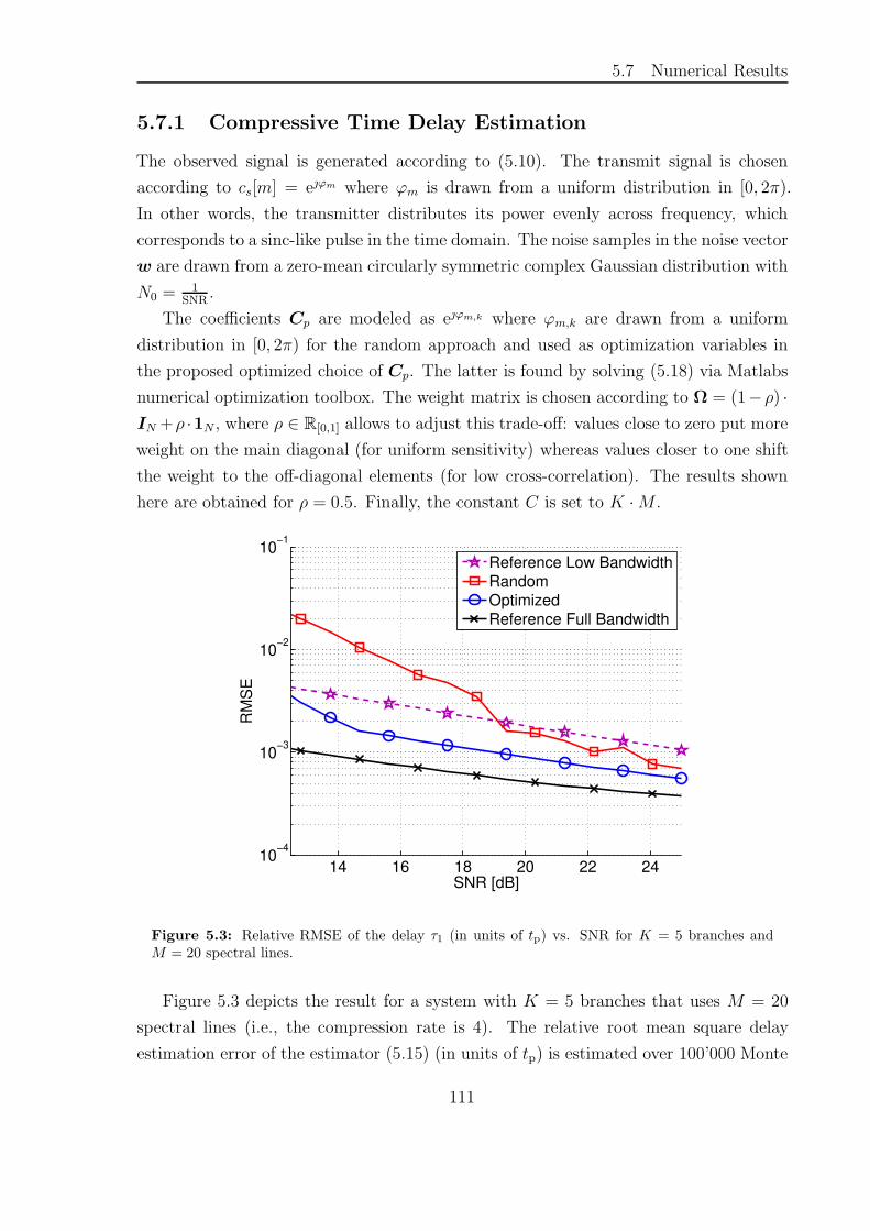
5.7 Numerical Results
5.7.1 Compressive Time Delay Estimation
The observed signal is generated according to (5.10). The transmit signal is chosen
according to cs[m] = eϕm where ϕm is drawn from a uniform distribution in [0, 2π).
In other words, the transmitter distributes its power evenly across frequency, which
corresponds to a sinc-like pulse in the time domain. The noise samples in the noise vector
w are drawn from a zero-mean circularly symmetric complex Gaussian distribution with
N0 =1
SNR.
The coefficients Cp are modeled as eϕm,k where ϕm,k are drawn from a uniform
distribution in [0, 2π) for the random approach and used as optimization variables in
the proposed optimized choice of Cp. The latter is found by solving (5.18) via Matlabs
numerical optimization toolbox. The weight matrix is chosen according to Ω = (1−ρ) ·IN +ρ ·1N , where ρ ∈ R[0,1] allows to adjust this trade-off: values close to zero put more
weight on the main diagonal (for uniform sensitivity) whereas values closer to one shift
the weight to the off-diagonal elements (for low cross-correlation). The results shown
here are obtained for ρ = 0.5. Finally, the constant C is set to K ·M .
14 16 18 20 22 2410
−4
10−3
10−2
10−1
SNR [dB]
RM
SE
Reference Low Bandwidth
Random
Optimized
Reference Full Bandwidth
Figure 5.3: Relative RMSE of the delay τ1 (in units of tp) vs. SNR for K = 5 branches andM = 20 spectral lines.
Figure 5.3 depicts the result for a system with K = 5 branches that uses M = 20
spectral lines (i.e., the compression rate is 4). The relative root mean square delay
estimation error of the estimator (5.15) (in units of tp) is estimated over 100’000 Monte
111

Chapter 5 Compressive Time Delay Estimation
Carlo trials. A single path scenario is chosen where α1 = 1 and τ1 is drawn randomly
from [0, tp). Since we have a single path, the correlation-based estimator according to
(5.14) is used to estimate the delays.
For comparison, the achievable accuracy of a traditional system that uses no com-
pression but a full-rate ADC is also shown (“Reference Full Bandwidth”) as well as the
performance of a system that uses 1/4 of the bandwidth (“Reference Low Bandwidth”).
The results demonstrate that the optimized measurement kernel outperforms the ran-
domly chosen one, in particular for lower SNRs. This behavior is mainly due to the
outliers that occur due to the sidelobes in the compressed correlation function. More-
over, the CS-based system achieves an accuracy better than a Nyquist system operating
with a reduced bandwidth / sampling rate.
To shed further light on this aspect, Figure 5.4 depicts the estimated complementary
cumulative distribution function (CCDF) of the RMSE for the same simulation at an
SNR of 13 dB. We can see that the random choice of the measurement kernels is more
prone to outliers. This behavior becomes even more pronounced for lower SNRs.
10−4
10−3
10−2
10−1
100
10−3
10−2
10−1
100
RSE
CC
DF
Reference Low Bandwidth
Random
Optimized
Reference Full Bandwidth
Figure 5.4: Histogram of the relative root squared error of τ1 for K = 5, M = 20, and an SNRof 13 dB.
Figure 5.5 shows the estimation result for a L = 6 path channel for K = 10,M = 20,
and an SNR of 30 dB, using the estimator from (5.13). The true value of delays and
amplitudes are indicated by the markers labeled “True” and compared to the proposed
112

5.7 Numerical Results
0 0.2 0.4 0.6 0.8 10
0.5
1
Delay τ/tp
Am
plit
ude
TrueReference Low BandwidthCompressedReference Full Bandwidth
Figure 5.5: Estimation of a multipath channel with L = 6 paths for K = 10, M = 20, SNR =30 dB
compressed approach (using an optimized matrix for ρ = 0.5) and the low/full band-
width reference.
The result shows that the compressed approach finds all the taps while the low
bandwidth version misses some peaks (and finds comparably strong spurious ones).
5.7.2 Compressive RBS Synchronization
We consider an OFDM signal as the opportunistic signal to be used for synchronization.
An L = 2048 sample window is recorded at each node. The reference signal is chosen
to be the first N = L/2 samples with D0 = L/4. The received signals at the kth node
and the reference node have a delay of dk = 36, and dref = 65 samples, respectively.
Therefore, the correlation peak is expected at the sample index ∆dk = D0 + dk −dref = 483. The additive noise vectors are drawn from a zero mean circularly symmetric
complex Gaussian distribution with variance PN, corresponding to a (pre-correlation)
signal to noise ratio (SNR) of 1/PN.
To implement our compressed correlation technique, we use a random compression
matrix Φ ∈ CM×N , where M is the length of the compressed signal to be communicated
throughout the network, i.e., the compressed signal has a bandwidth of MN·B = B
R, where
R = N/M denotes the compression rate. The coefficients of Φ are drawn from a zero
mean circularly symmetric complex Gaussian distribution as well where each element
has variance 1N.
Figure 5.6 shows the correlation functions computed using the proposed compressed
design for an SNR of 0 dB (for clarity, only the region around the correlation peak is
shown).
113

Chapter 5 Compressive Time Delay Estimation
472 474 476 478 480 482 484 4860
0.2
0.4
0.6
0.8
1
Sample index
Co
rre
latio
n
Full Bandwidth
Compressed R = 2
Compressed R = 4
Compressed R = 8
Figure 5.6: Comparison of the correlation function ρ(c)k [∆d] at a node k with ∆dk = 483 for
different compression rates R.
−10 −8 −6 −4 −2 00
0.2
0.4
0.6
0.8
1
Pro
babili
ty o
f success
SNR [dB]
Full Bandwidth
Compressed R = 2
Compressed R = 4
Compressed R = 8
Figure 5.7: Empirical probability of correctly detecting the main correlation peak vs. the SNRfor different compression rates R.
114

5.8 Summary
For comparison, the graph labeled “Full Bandwidth” shows the result when the
reference node sends an uncompressed (high bandwidth) copy of the opportunistic signal
to all nodes and they use that to obtain the correlation. As expected, the compressed
designs achieve almost the same accuracy as the high bandwidth system (i.e., they all
have a peak at the correct delay ∆dk = 483) at a much lower bandwidth. Figure 5.6
also shows that higher compression leads to higher side lobes.
To further analyze this behavior, we have conducted an additional experiment shown
in Figure 5.7. Here, we vary the SNR by scaling all the noise samples to variance 1/SNR.
We compute the empirical probability that the main correlation peak is identified at the
correct location, i.e., Pr[∆dk = ∆dk]. The empirical probabilities are averaged over
500 trials where each trial represents a new realization of the noise samples as well as
the compression matrix Φ. Higher compressions move the curve to higher SNRs. This
means that to achieve the same success rate a larger SNR is required when compared
to the uncompressed approach. This can be explained according to (5.26) where the
correlation between the columns of the compression matrix rises and henceΦHΦ deviates
stronger from the identity matrix, distorting the shape of the correlation function.
5.8 Summary
In this chapter, we have investigated a system architecture for delay estimation via
Compressed Sensing (CS). We propose to use a bank of K periodic functions pk(t) that
multiply the received signal and are sampled once per period. Thereby, the effective
sampling rate is reduced by a factor which depends on the period, the bandwidth, and
the number of channels K.
We then discuss the design of the functions pk(t) based on their frequency domain
representation. We propose an approach that directly optimizes the shape of the auto-
correlation function in terms of the choice of pk(t) and demonstrate that it outperforms
a random choice in terms of the delay estimation accuracy.
We have also discussed a compressed technique for temporal synchronization with
high bandwidth opportunistic signals. The main idea is to let the reference node transmit
a compressed form of the reference signal for synchronization and thus reducing the data
rate needed for communication between the nodes.
We proposed a random design of the compression matrix inspired by the compressed
sensing findings about designing measurement ensembles that preserve the information
rate of the original system. We have shown that the compression does not significantly
affect the correlation function obtained at the receiving nodes compared to the high
115

Chapter 5 Compressive Time Delay Estimation
bandwidth correlation functions obtained from the original non-compressed reference
However, the expense for the reduction in bandwidth is an increased sidelobe level
of the correlation function. This effect mirrors a degradation in the effective SNR which
means that there is a tradeoff between the bandwidth reduction and the SNR that can
be controlled by the compression ratio.
116

Chapter 6
Compressive Spatial Channel
Sounding
This chapter deals with the application of compressive arrays discussed in Chapter 4
to channel sounding. After the motivation in Section 6.1, the main channel sounding
principles are summarized in Section 6.2. In Section 6.3, the usage of compressive arrays
for spatial channel sounding is investigated and then evaluated by numerical simulations
based on a real scenario in Section 6.4. The chapter is then summarized in Section 6.5.
6.1 Motivation
Electromagnetic (EM) wave propagation between transmitter (TX) and receiver (RX)
antennas undergoes a variety of interactions with the objects of the environment leading
to multiple propagation paths that are spread in directions of departure (DoD) and
arrival (DoA), time delay and Doppler. Proper handling of this multipath diversity is
the key enabler to achieve high data rate, robust operation and ubiquitous coverage
in mobile radio. Therefore, the multidimensional structure of electromagnetic wave
propagation has to be studied, analyzed, and identified.
Multidimensional channel sounding is the key technology for experimental analysis
of electromagnetic wave propagation in mobile radio channels [235]. A channel sounder
is a multidimensional data recording system, which measures and identifies the multi-
path propagation structure in mobile radio. These measurement results are required for
experimental studies of multipath propagation, channel modeling and mobile radio sys-
tem performance prediction. If conventional Nyquist schemes are applied, the recorded
data volume is determined by the number of antenna array elements at TX and the RX,
the length of the channel impulse response and the number of the observed snapshots
117

Chapter 6 Compressive Spatial Channel Sounding
over slow time. A wide variety of high resolution parameter estimation (HRPE) is avail-
able [19] to estimate these structural parameters by fitting an appropriate data model
to the recorded data.
The number of measurements is orders of magnitude larger than the number of pa-
rameters. This suggests that there is a significant amount of redundancy (sparsity) in
the recorded signals. In this chapter, it is our goal to take advantage of compressive sens-
ing (CS) [30,31,101] to reduce the amount of data stored and the hardware complexity
without losing any relevant information but saving a huge part of resources. Moreover,
snapshot recording time (and thus repetition time) can be considerably reduced (e.g., by
minimizing the number of recorded Tx/Rx MIMO links). This allows better handling of
dynamic scenarios (i.e., increasing the Doppler range) which is still the highest challenge
in MIMO channel sounding.
The application of CS to channel sounding is hardly described in literature. A
Channel Sounding Xampler was proposed in [236] based on the sub-Nyquist Xampling
architecture [237] reducing the measurement acquisition time while simultaneously es-
timating time delays, multipath amplitudes, and angles of arrival. However, the main
focus was to reduce the sampling effort in the time-frequency domain by exploiting the
sparsity of the channel there. Otherwise, related ideas can be found in the application
of compressed sensing to MIMO radar [238] and compressive channel sensing [46].
In this chapter, we exploit the application of CS to the double-directional channel
sounder in the spatial domain that includes joint DoA/DoD estimation. In particular,
the CS paradigm can be implemented in the spatial domain by employing M antenna
elements that are combined into a smaller number of m < M active RF chains using
an analog combining network (at the transmitter, the receiver or both). Since only m
channels need to be sampled and digitized, the hardware complexity remains comparably
low while allowing us to cover a larger aperture (and thus be more selective) than a
traditional, Nyquist (λ/2) spaced m-channel antenna array. Based on the fact that
the underlying signal is sparse in the angular domain, CS theory suggests that it can
be recovered from m < M measurements, provided that the measurement kernel is
appropriately chosen.
A compressive spatial channel sounder is proposed and evaluated based on real sce-
narios showing superior advantages in terms of time, hardware complexity and resolu-
tion. In particular, the proposed approach reduces the total number of switching peri-
ods, which implies a reduced channel acquisition time and thus an improved Doppler
bandwidth. On the other hand, the compressive approach reduces the number of RF
chains, which is a very relevant advantage in terms of the overall receiver complexity,
118

6.2 Channel Sounding
the amount of data to be processed in the digital domain (e.g., FPGA), power consump-
tion, as well as RF hardware calibration. Alternatively, for the same measurement time
and/or hardware complexity, one can increase the number of array elements to cover a
larger aperture and so achieving better performance in terms of resolution.
6.2 Channel Sounding
The definition of the channel sounding data model is crucial for parameter estimation.
It has to represent the reality of wave propagation and the influence of the measurement
device. We prefer a data model comprising two components which can be handled
separately throughout the estimation procedure. The first part is deterministic and
results from specular-like reflections. The second part represents distributed diffuse
scattering which typically occurs in a complicated, multipath rich environment. We
focus on the first part and leave the second for future works (see e.g., [239] for more
details about handling diffuse scattering).
Consider measuring the channel transfer function between two points in space (nTX
for the n-th antenna array element at the transmitter and mRX for the m-th receiver
element) inside a certain bandwidth. A simplified model for the channel in the mul-
tidimensional aperture domain is given by a superposition of a discrete number of S
propagation paths [240].
Expressed in the frequency domain, we can write
h(f,mRX, nTX) =S∑
s=1
γs · e−2πfτs · gm,RX(Ωs,RX) · gn,TX(Ωs,TX), (6.1)where f
denotes the frequency, γs ∈ C and τs ∈ R are the amplitude and delay of the s-th path,
Ωs,RX and Ωs,TX denote the Direction-of-Arrival (DoA) and Direction-of-Departure
(DoD), in general in both azimuth and elevation domain, of the s-th path at the receiv-
ing and the transmitting side. Moreover, gm,RX and gn,TX denote the complex radiation
pattern of the m-th receiver and n-th transmitter element, respectively1. The complex
patterns describe the gain of the antenna itself as well as the phase shift caused by the
geometrical arrangement within the antenna array.
The temporal and frequency characteristics are measured by exciting the channel
with a well defined transmit signal. The channel impulse response is obtained by post-
processing the recorded data, depending on the type of transmit signal. Common types
of signals are pseudo-noise sequences with subsequent correlation of the measured data
1In general they will depend on frequency f as well but we assume here that the bandwidth is nottoo high.
119

Chapter 6 Compressive Spatial Channel Sounding
with the transmit sequence as well as specially designed periodic multi-tone signals. The
benefit of multi-tone signals is the easier control of the occupied bandwidth (theoretically,
it is rectangularly shaped). Furthermore, the transmit signal can be removed from the
recorded data (deconvolution of the transmit signal) by a simple division in the frequency
domain. This step can be combined with the calibration of the RF equipment resulting
in very little additional effort.
For measuring the spatial properties of the channel, MIMO channel sounders are
used. They feature antenna arrays at both the transmitter and receiver side. Specif-
ically, double-directional measurements that include joint DoA/DoD estimation allow
the separation of the directional dependent influence of the measurement antennas from
the channel measurements which is a prerequisite of antenna-independent channel char-
acterization [235].
In theory, all combinations of transmitter and receiver array elements can be mea-
sured at the same time and frequency. While this can be achieved with parallel RF
chains at the receiver, it is not meaningful to excite all transmitter elements with the
same signal at the same time, due to the inability to distinguish the different transmit-
ters at the receiver. To be able to separate TX antennas, one has to choose transmit
sequences that are at least linearly independent over the antennas (or better yet, orthog-
onal). These can be Code, Frequency, or Time Division Multiplexing (CDM or FDM
or TDM) or combinations thereof. The most established technique is Time Division
Multiplex (TDM). TDM based sounders measure the response from each TX antenna
element separately by switching. During a specific time frame, only a single transmitter
antenna element is active. For this reason, TDM only needs one TX RF chain followed
by a switch, which makes it very attractive from the hardware complexity point of view.
We therefore focus on TX TDM exclusively in this paper.
For the measurement at the receiver, we have two main options. The first is to let
all M RX antennas listen jointly which then requires M RF chains. The other option is
to apply receive switching as well. The advantage of the latter is the use of a single RF-
chain and ADC/DAC which relaxes the requirements of the RF calibration dramatically.
However, the price we pay is anM times longer measurement time. Intermediate options
between the two extremes are possible as well, which allows us to control the trade-off
between the hardware complexity and the measurement rate (which controls the Doppler
bandwidth we can cover).
At TU Ilmenau, a MIMO channel sounder is available which is designed following the
TDM principle [241, 242] at TX and RX. The RUSK-HyEff-Sounder was used through-
out numerous channel sounding campaigns where a variety of different antenna arrays
120
6.3 Compressive Spatial Channel Sounding
suitable for high resolution parameter estimation were employed. The obtained data
was used to directly evaluate the performance of different MIMO systems [243], as well
as an input for calculating parameters of the channel model [244].
6.3 Compressive Spatial Channel Sounding
The number of array elements and the choice of the antenna array geometry heavily
determines the performance of any subsequent high resolution parameter estimation
algorithm. According to the spatial sampling theory, the distance between adjacent sen-
sors should be less than or equal to half a wavelength of the impinging planar wavefronts,
otherwise it leads to grating lobes (sidelobes) in the spatial correlation function which
correspond to near ambiguities in the array manifold. At the same time, to achieve
DoA/DoD estimation with a high resolution, the receiving arrays should have a rela-
tively large aperture [28]. This implies that arrays with a large number of antennas are
needed to obtain a high resolution, which then requires complex hardware processors
and/or long measurement times. The main goal of this work is to exploit the sparsity
of the channel in the spatial domain considering only the specular-like components of
the channel towards reducing that measurement complexity (i.e., hardware and time).
Recently, compressed sensing (CS) has been widely suggested for applications that ex-
hibit sparsity in space to reduce the measurement efforts and/or improve the estimation
performance (i.e., spatial resolution). It is highlighted in [29] that if the electromagnetic
field is modeled as a superposition of a few plane waves, the DoA/DoD estimation prob-
lem can be expressed as a sparse recovery problem. Since then, many sparse recovery
algorithms became popular in the CS field for the DoA/DoD estimation problem as an
alternative to existing parameter estimation algorithms [175, 176]. On the other hand,
there has been comparably little research towards applying the CS paradigm spatially
to antenna arrays. Yet, this is an attractive idea since the sampling of RF signals is
a costly task as each receiver chain requires hardware components such as low-noise
amplifiers, filters, mixers, and A/D converters. Therefore, reducing the number of chan-
nels that have to be sampled could significantly lower the hardware complexity and the
measurement time [8,45,150]. In this work, we extend this idea to the double directional
MIMO scenario with antenna arrays at both the transmitter and the receiver. We focus
on the spatial domain where the ultimate goal is to estimate the DoAs and the DoDs.
Consider a multipath channel scenario with S paths. A MIMO channel sounder is
used with N transmit antennas and M receive antennas. For a single snapshot and
121

Chapter 6 Compressive Spatial Channel Sounding
assuming only a narrowband scenario, the channel can be written as:
h(mRX, nTX) =S∑
s=1
γs · am,RX(Θs,RX) · an,TX(Θs,TX), (6.2)
where γs ∈ C and τs ∈ R are the amplitude and delay of the s-th path, Ωs,RX and
Θs,TX denote the Direction-of-Arrival (DoA) and Direction-of-Departure (DoD) in the
azimuth domain, of the s-th path at the receiving and the transmitting side. Moreover,
am,RX and an,TX denote the array response of the m-th receiver and n-th transmitter
element, respectively.
In matrix notation, one can write
H = ATRX · Γ ·ATX, (6.3)
where H ∈ CM×N represents the channel transfer function in the spatial domain, Γ is
a diagonal matrix with the paths’ power on the main diagonal, ARX and ATX are the
array steering matrices for the receive and transmit arrays respectively.
The main idea of spatial CS is that instead of measuring each antenna separately,
we sample only a linear combination of the signals from all the antennas. Such linear
combinations can be implemented in the analog domain, e.g., via networks of power
dividers and phase shifters (see [8] for more details).
For channel sounding, we apply this idea at both the TX and the RX. For the TX,
this means that instead of transmitting from one antenna at a time and cycling through
all antennas, we transmit via a set of beams, where each beam represents a complex
weight vector applied to the TX antennas. We can write this as a sequence of transmit
signals ϕTX,k · sk, k = 1, 2, . . . , n, where ϕTX,k ∈ CN and sk are the weight vector and
the transmit symbol in the k-th TX switching period, respectively.
At the receiver, instead of measuring the antenna signals directly, we form linear
combinations via receive weight vectors denoted as ϕRX,ℓ ∈ CM , which can again be
implemented as an analog beamforming network. Here, ℓ = 1, 2, . . . , m represents the
receive measurement index. After cycling through all n TX beams and all m RX weight
vectors, we have collected a total number of n ·m compressive observations which we
can write as
Hc = ΦTRX ·AT
RX · Γ ·ATX ·ΦTX, (6.4)
whereHc ∈ Cm×n denotes the compressive spatial channel transfer function and ΦRX ∈
122

6.3 Compressive Spatial Channel Sounding
Cm×M and ΦTX ∈ Cn×N represent the RX and TX combining matrices which contain
the vectors ϕRX,ℓ and ϕTX,k, respectively.
Compared to the Nyquist approach, this reduces the total number of observations
from M · N to m · n where n < N and m < M . This implies some relevant practical
benefits. First of all, the proposed approach reduces the total number of TX switch-
ing periods to n < N , which implies a reduced channel acquisition time and thus an
improved Doppler bandwidth. For the receiver, the concrete advantage depends on the
implementation choice which was discussed in Section 6.2. If we choose to employM RX
RF chains, the compressed approach reduces the number of RF chains to m < M , which
is a very relevant advantage in terms of the overall receiver complexity, the amount of
data to be processed in the digital domain (e.g., FPGA), power consumption, as well
as RF hardware calibration. If we choose to measure the RX chains sequentially and
employ receive switching, the compressive approach reduces the number of measurement
cycles further compared to Nyquist since instead of M · N we then only require m · ncycles.
Note that another advantage of such a compressive architecture is that it allows us to
reconfigure the array on the fly without any change in the receiver hardware which can
be very advantageous in many applications. In [45] and its follow-up papers, it has been
suggested to consider measurement kernels Φ drawn from random distributions such
as Gaussian or Bernoulli distributions. Such a choice is popular due to its simplicity
and certain mathematical guarantees on the uniform support recovery, i.e., recovering
arbitrary subsets of K non-zero entries in s(t). In our recent works [4,8], we have shown
that optimizing Φ can improve the performance significantly. We will compare different
constructions of Φ via simulations and discuss their implementation.
After having the compressive measurements, the same ML-based estimators (e.g.,
The RIMAX [245]) could be applied to multidimensional channel parameter estimation
from field experiments. In this paper, our goal is to evaluate the performance of recov-
ering the channel parameters from noisy observations. To this end, the performance
metrics we consider are the conditional (deterministic) Cramer-Rao Bounds (CRBs) as
a proxy to the performance of ML-type estimators. This is done since ML estimators
are known to (asymptotically) achieve the CRB and therefore it provides an abstrac-
tion over the concrete ML implementation. Moreover, the computation of the CRBs
is much simpler allowing for larger ensembles to be considered. In addition, since the
compression is a linear operation, it is very easy to find the CRB for the compressed
model (6.4), cf. [8]. Future works would feature direct application of an ML-based esti-
mator to the compressive measurements from realistic scenarios towards obtaining the
123

Chapter 6 Compressive Spatial Channel Sounding
channel parameters.
6.4 Numerical Simulations
In this section, we present some numerical results to demonstrate the compressive spa-
tial channel sounding concept and evaluate its advantages compared to conventional
sounding. At TU Ilmenau, a MIMO channel sounder is available which is designed fol-
lowing the TDM principle at the TX and the RX. The sounder was used throughout
numerous channel sounding campaigns where a variety of different antenna arrays suit-
able for high resolution parameter estimation were employed. We consider a realistic
scenario based on a sounding campaign of the RESCUE project [246] at the campus of
TU Ilmenau. Here, a V2V-type setup was considered at the campus of the TU Ilmenau
at 2.35 GHz carrier frequency and 36 dBm transmit power. The antenna arrays used
at both the transmitter and receiver are two 16-element Stacked Polarimetric Uniform
Circular Array (SPUCA) placed on two trolleys. The main purpose is to investigate the
impact of a moving transmitter on the channel observed by the receiver. Therefore, a
grid of transmitter locations was selected where the grid points are separated by 10m on
each lane (two adjacent grid points on the same lane are 10m apart). The transmitter
was located on each of the grid points and the receiver was slowly moved on the opposite
lane. Figure 6.1 shows the grid positions of the TX and the RX where the black circle
highlights the positions we use for our simulations.
After the measurement campaign, we have ran the recorded data through the ML-
based high-resolution parameter estimation scheme RIMAX [245] to extract the param-
eters of the individual propagation paths. In particular, for each path, its DoA, DoD
(azimuth and elevation), delay, and polarimetric path weights were estimated. This al-
lows to remove (de-embed) the effect of the antenna array that was used to measure the
channel. It also allows to resynthesize the channel with a reduced number of relevant
paths to simplify its complexity.
Since this paper presents a first study on the possibility of applying spatial CS to
the sounding problem without considering all the dimensions (e.g., frequency), the main
goal of the numerical evaluation is to provide a proof of concept. We therefore simplify
the complexity of the channel significantly by considering only the four dominant paths
for a specific TX/RX position and for a single snapshot. Focusing only on the spatial
domain, we aim at estimating the DoAs and the DoDs shown in Figure 6.2. Note how
there are two paths that are very closely spaced in terms of their DoA, which makes it
challenging to resolve them.
124

6.4 Numerical Simulations
Figure 6.1: Top view of the locations of the transmitter and the receiver during the measurementcampaign considered.
-100 -50 0 50 100
DoDs
-100
-50
0
50
100
150
DoA
s
Figure 6.2: The DoAs and the DoDs of the 4 most dominant paths for the considered scenario.
125

Chapter 6 Compressive Spatial Channel Sounding
CRB Ratio
10-2
10-1
100
CC
DF
0
0.1
0.2
0.3
0.4
0.5
0.6
0.7
0.8
0.9
1
Large (M=N=32)
Gaussian (m=n=16)
Rademacher (m=n=16)
Random Phase (m=n=16)
Switching (m=n=16)
Optimized (m=n=16)
Figure 6.3: The CCDF of the mean CRB of the DoAs and DoDs for 10000 random realizationsof ΦTx and ΦRx with 4 different designs.
As mentioned earlier, the performance of the compressive sounder will be evaluated
based on the CRBs of the DoA/DoD estimation as a proxy to the performance of ML-
type estimators. Figure 6.3 studies the performance of the compressive spatial channel
sounder for DoD/DoA estimation and compare it to the uncompressed cases. For the
case where we have a full array (i.e., fully meshed with no combining network) with
16 TX array elements and 16 RX array elements, the mean CRB of the DoAs and
the DoDs is calculated and then used as a reference onward. Let’s call this CRBsmall.
The large array is the one where we have 32 elements instead of 16 which we then call
CRBlarge. The compressed case is the one where we have 32 antenna elements but only
16 measurements (and/or 16 RF channels) and this we call CRBcompressed. The mean
CRB values are calculated for both cases (i.e., the large array and the compressed one)
and then normalized to the mean CRB of the small array for comparison. We call
this the CRB Ratio where the CRBlarge and the CRBcompressed shown are normalized to
CRBsmall (e.g., CRB Ratio =CRBlarge
CRBsmall). The main advantage of this ratio is that it is
independent of the SNR. No matter what’s the SNR, we will always have this factor in
variance reduction in the CRBs.
The coefficients of the combining networks ΦTx and ΦRx are then selected according
to 5 different criteria which we name Gaussian, Rademacher, Random Phase, Switching
126

6.4 Numerical Simulations
and Optimized. The complementary cumulative distribution function (CCDF) for 10000
realizations of the random combining networks is shown (i.e., the Gaussian; the Random
Phase, the Rademacher, and the Switching). In the Gaussian case, the coefficients are
drawn from a from a zero mean circularly symmetric complex Gaussian distribution. In
the Random Phase case, a unit norm is chosen while the phases are drawn uniformly
at random from (0, 2π]. The Rademacher setup is the one where the coefficients are
drawn randomly from a Rademacher distribution with only ±1s as possible outcomes
at a 50% chance. The switching design is the one where for each measurement, one TX
and one RX antenna/port is selected at random. The optimized design is the one we
recently proposed based on optimizing the spatial correlation functions for DoD/DoA
estimation [4].
The results show that the optimized design is the best 90% of the cases while the
switching case is the worst. The Gaussian, the Random Phase and the Rademacher
constructions achieve similar performance. However, from an implementation point of
view, the switching design is the most appealing and realizable one where only a switch
is needed to construct the network (one at the TX and one at the RX). The Rademacher
design with only ±1s requires only adders and inverters (180 phase shifters) to realize,
which make them the second choice to implement. Both the Random Phase and the
Optimized cases require phase shifters with an almost continuous phase range which
make them very challenging to realize. The Gaussian case with a varying amplitude
would make the implementation even more challenging and so that is why it is better
to avoid it. We are currently investigating the optimization of the combining network
with regard to the implementation challenges as well as the estimation performance.
The figure shows that the CRB of the compressive array is not as good as that of the
full large array of 32 elements but still much better (more than 10 times better) than
that of the uncompressed, conventional 16-element array. In case of a TDM TX/RX
architecture, this means lower measurement time compared to the full 32 array case.
Instead of taking 32× 32 = 1024 measurement cycles, only 16× 16 = 256 (i.e., only 1/4
the number of measurements compared to the full array) would suffice and so increasing
the Doppler range without degrading the performance drastically. This can be of great
importance when considering fast varying channels with a large Doppler spread. In
case of a TDM TX and a linear combining compressive RX, we do 16 × 32 = 512
measurements and reduce the hardware complexity to 16 < 32 RX RF chains.
Alternatively, for the same measurement time and/or hardware complexity, one can
increase the number of array elements to cover a larger apperture and so achieve better
performance in terms of resolution. Figure 6.4 shows the improvement in the CRBs
127

Chapter 6 Compressive Spatial Channel Sounding
CRB Ratio
10-3
10-2
10-1
CC
DF
0
0.1
0.2
0.3
0.4
0.5
0.6
0.7
0.8
0.9
1
Large (M=N=32)
Compressed (M=N=32 => m=n=16)
Large (M=32,N=64)
Compressed (M=32,N=64 => m=n=16)
Large (M=32,N=128)
Compressed (M=32,N=128 =>m=n=16)
Figure 6.4: The improvement in the CRBs using larger number of array elements at the RX witha fixed number of 32 elements at the TX.
proportional to increasing the number of array elements (the Rademacher design is used
to obtain ΦTx and ΦRx). The TX has 32 elements with a combining network of only
16 measurements. The RX takes only 16 compressive measurements but the number of
elements is varied from 32 to 64 to 128 elements. The CRBs of the DoA/DoD estimation
improves (i.e., reduces) significantly while keeping the measurement complexity the same
(i.e., 16 measurements). This can be interpreted as increasing the array aperture by using
more antenna elements at the RX and so achieving a better resolution.
6.5 Summary
In this chapter, we consider the application of compressive sensing (CS) to channel
sounding in the spatial domain. We proposed a compressive spatial channel sounding
architecture where the antenna elements at the transmitter, the receiver or both are
combined into a smaller number of channels using an analog combining network. The
proposed approach reduces the total number of switching periods, which implies a re-
duced channel acquisition time and thus an improved Doppler bandwidth. On the other
hand, the number of RF chains can be reduced, which is a very relevant advantage
in terms of the overall receiver complexity, the amount of data to be processed in the
128

6.5 Summary
digital domain (e.g., FPGA), power consumption, as well as RF hardware calibration.
Alternatively, for the same measurement time and/or hardware complexity, one can in-
crease the number of array elements to cover a larger aperture and so achieving better
performance in terms of resolution. Based on a realistic scenario, we show by simulations
the superiority of the proposed compressive architecture in terms of the measurement
complexity (i.e., time and hardware) and/or estimation performance.
129

Chapter 6 Compressive Spatial Channel Sounding
130

Chapter 7
Conclusions
This chapter concludes this thesis and summarizes its main contributions.
Thesis summary
In this thesis, the application of compressive sensing (CS) to the problem of direction
of arrival (DOA) estimation has been examined and its applicability to the time delay
(TD) estimation and channel sounding has been investigated. The major objective
was to develop approaches that allow to minimize the hardware complexity in terms
of receiver costs and power consumption, while providing a desired level of estimation
accuracy and robustness in the presence of multiple sources and/or multiple paths.
We started in Chapter 2 by providing the background related to the work in this
thesis. We mainly discussed the underlying principles of CS and DOA estimation.
Chapter 3 addressed the problem of CS-based DOA estimation for off-grid sources.
We studied the spectrum in the case of off-grid sources qualitatively and found that
most of the energy of the off-grid source after reconstruction is concentrated in the
two neighboring grid points. Based on this observation, we derived the best two-term
approximation coefficients explicitly and showed that the approximation error is very
small. Moreover, we proposed a very simple scheme to estimate the grid offset based on
the observed coefficients. For multiple sources, we showed that this simple scheme still
works well when they are sufficiently spaced. For closely spaced sources, we proposed a
numerical procedure for the joint estimation of their offsets from the recovered spectra
at their neighboring grid points. Afterwards, the CS-based formulation of the DOA
estimation problem has been extended to the polarimetric model. We discussed the off-
grid problem in the polarimetric setting and proposed an estimator for the grid offset
of one source (or an isolated source) as well as a joint estimator for the grid offsets
131

Chapter 7 Conclusions
of two closely-spaced sources. Our numerical results demonstrated that the estimators
could recover the DOA regardless of the polarization state of the incoming wave and is
applicable to arbitrary arrays.
In Chapter 4 we investigated the application of CS in the spatial domain via com-
pressive arrays that aim to provide a larger aperture with a reduced hardware complexity.
We presented an architecture of such a compressive array and introduced a generic sys-
tem model that included different options for the hardware implementation. We then
focused on the choice of the coefficients in the analog combining network. We started by
demonstrating that choosing it randomly may lead to undesirable effects in the effective
CS array such as very high sidelobes. Instead of choosing them randomly, we proposed
a generic design approach for the analog combining network with the goal to obtain
an array with certain desired properties, e.g., uniform sensitivity, low cross-correlation,
or low variance in the DOA estimates. Our numerical simulations demonstrated the
superiority of the proposed optimized compressive arrays to compressive arrays with
randomly chosen combining kernels and to a sparse array of the same complexity. Also
our proposed compressive array enjoys a high degree of adaptability since the combining
weights can be altered to adjust the array to the current requirements, which is impossi-
ble for sparse arrays due to their static nature. We have also proposed a focusing design
of the compression matrix which resulted in a significant performance improvement com-
pared to the uniform design. Moreover, we proposed an extension for the combining
matrix design for 2D (elevation and azimuth) DOA estimation with compressive antenna
arrays.
Finally, we considered two other applications of the proposed approaches namely, CS
based time delay (TD) estimation and compressive channel sounding. In Chapter 5,
we investigated a CS based system architecture for TD estimation. We proposed to use a
bank ofK periodic functions pk(t) that multiply the received signal and are sampled once
per period. Thereby, the effective sampling rate is reduced by a factor which depends on
the period, the bandwidth, and the number of channels K. We then discussed the design
of the functions pk(t) based on their frequency domain representation. We proposed an
approach that directly optimizes the shape of the autocorrelation function in terms of
the choice of pk(t) and demonstrate that it outperforms a random choice in terms of the
delay estimation accuracy.
Chapter 6 considered the application of CS to channel sounding in the spatial
domain. We proposed a compressive spatial channel sounding architecture where the
antenna elements at the transmitter, the receiver or both are combined into a smaller
number of channels using an analog combining network. The proposed approach reduces
132

the total number of switching periods, which implies a reduced channel acquisition time
and thus an improved Doppler bandwidth. On the other hand, the number of RF chains
can be reduced, which is a very relevant advantage in terms of the overall receiver
complexity, the amount of data to be processed in the digital domain (e.g., FPGA),
power consumption, as well as RF hardware calibration. Alternatively, for the same
measurement time and/or hardware complexity, one can increase the number of array
elements to cover a larger aperture and so achieving better performance in terms of
resolution. Based on a realistic scenario, we showed by simulations the superiority of
the proposed compressive architecture in terms of the measurement complexity (i.e.,
time and hardware) and/or estimation performance.
Contributions
The main contributions of this thesis are:
A qualitative analysis of the model mismatch for CS based DOA estimation off
the grid based on the shape of the resulting spectrum.
A simple scheme for CS based DOA estimation off the grid for one source as well
as multiple sources based on the aforementioned analysis.
A novel polarimetric based CS based DOA estimation off the grid while polariza-
tion has been almost always ignored by state-of-the-art CS based DOA estimation
methods.
A basic architecture of a compressive array employing linear combinations in the
analog domain by means of a network of power splitters, phase shifters, and power
combiners with a generic system model that includes different options for the
hardware implementation.
An efficient design of the combining matrix to obtain an array that is suitable
for DOA estimation (i.e., minimum variance of DOA estimates and robustness in
terms of low side lobe levels or low probability of false detections).
An extension of the presented ideas to be applied in TD estimation and synchro-
nization. We mainly proposed an optimization based design for the measurement
kernels of the CS based TD estimation architectures. We also proposed a CS based
reference broadcast synchronization where the reference signal is an opportunistic
signal already in the system (e.g., FM or TV signals).
133

Chapter 7 Conclusions
A compressive spatial channel sounder is proposed and evaluated based on real
scenarios showing superior advantages in terms of time, hardware complexity and
resolution.
Closing remarks
Compressive sensing and sparse recovery techniques have opened up new horizons for
DOA estimation with sensor arrays. For almost a decade now, many CS based DOA esti-
mation approaches have been proposed that allow to minimize the hardware complexity
in terms of receiver costs, measurement time and power consumption, while providing a
superior estimation accuracy and robustness in the presence of multiple sources and/or
multiple paths.
This thesis tackled two main challenges of CS based DOA estimation, namely: the
sparse CS based recovery of offgrid sources and the design of the combining network
for compressive arrays. We have studied both problems quantitatively and proposed
efficient schemes towards solving them. We have also shown the possible extension of
these ideas to other applications, mainly: TD estimation and channel sounding.
134

Bibliography
Own Publications
[1] F. Romer, R. Alieiev, M. Ibrahim, G. Del Galdo, and R. S. Thoma. An ana-lytical study of sparse recovery algorithms in presence of an Off-Grid source. InInternational Workshop on Compressed Sensing applied to Radar, Bonn, Germany,September 2013.
[2] M. Ibrahim, F. Romer, R. Alieiev, G. Del Galdo, and R. S. Thoma. On theestimation of grid offsets in cs-based direction-of-arrival estimation. In Interna-tional Conference on Acoustics, Speech and Signal Processing (ICASSP), pages6776–6780, May 2014.
[3] F. Romer, M. Ibrahim, R. Alieiev, M. Landmann, R. S. Thoma, and G. Del Galdo.Polarimetric compressive sensing based DOA estimation. ITG Workshop on SmartAntennas (WSA), March 2014.
[4] M. Ibrahim, F. Romer, and G. Del Galdo. On the design of the measurementmatrix for compressed sensing based doa estimation. In International Conferenceon Acoustics, Speech and Signal Processing (ICASSP), pages 3631–3635, April2015.
[5] S. Skoblikov, M. Ibrahim, F. Romer, R. S. Thoma, and G. Del Galdo. Doa estima-tion with reflectarray according to single pixel camera principle. In InternationalWorkshop on Compressed Sensing Theory and its Applications to Radar, Sonarand Remote Sensing (CoSeRa), pages 268–272, Jun 2015.
[6] S. Skoblikov, M. Ibrahim, F. Romer, and R. S. Thoma. Numerical assessmentof reflectarray applicability to cs-based doa estimation. In International RadarSymposium (IRS), pages 404–409, June 2015.
[7] M. Ibrahim, F. Romer, and G. Del Galdo. An adaptively focusing measurementdesign for compressed sensing based doa estimation. In European Signal ProcessingConference (EUSIPCO), pages 859–863. IEEE, 2015.
135

[8] M. Ibrahim, V. Ramireddy, A. Lavrenko, J. Konig, F. Romer, M. Landmann,M. Grossmann, G. Del Galdo, and R. S. Thoma. Design and analysis of compres-sive antenna arrays for direction of arrival estimation. Signal Processing, 138:35 –47, 2017.
[9] A. Lavrenko, S. Pawar, M. Ibrahim, F. Romer, G. Del Galdo, and R. S. Thoma.Combining matrix design for 2d doa estimation with compressive antenna arrays.ITG Workshop on Smart Antennas (WSA), March 2017.
[10] M. Ibrahim, F. Romer, N. Hadaschik, H. M. Troger, B. Sackenreuter, N. Franke,J. Robert, and G. Del Galdo. Compressed temporal synchronization with oppor-tunistic signals. Radio Wireless Week, Nov 2015.
[11] M. Ibrahim, F. Romer, N. Hadaschik, H. M. Troger, B. Sackenreuter, N. Franke,J. Robert, and G. Del Galdo. Temporal wireless synchronization with compressedopportunistic signals. Radio Wireless Week, Jan 2016.
[12] F. Romer, M. Ibrahim, N. Franke, N. Hadaschik, A. Eidloth, B. Sackenreuter,and G. Del Galdo. Measurement matrix design for compressed sensing based timedelay estimation. In European Signal Processing Conference (EUSIPCO), pages458–462, Aug 2016.
[13] M. Ibrahim, W. Al-Aqqad, F. Romer, M. Kaske, S. Semper, R. S. Thoma, andG. Del Galdo. Compressive spatial channel sounding. In European Conference onAntennas and Propagation, London, UK, April 2018.
References by Other Authors
[14] Ericsson AB. Ericsson Mobility Report. White paper, 2017.
[15] D. H. Johnson and D. E. Dudgeon. Array Signal Processing: Concepts and Tech-niques. Simon & Schuster, Inc., New York, NY, USA, 1992.
[16] R. A. Monzingo and T. W. Miller. Introduction to adaptive arrays. Scitech Pub-lishing, 1980.
[17] M. I. Skolnik. Introduction to Radar Systems. McGraw Hill Book Co., New York,2 edition, 1980.
[18] L. C. Godara. Application of antenna arrays to mobile communications. ii.beam-forming and direction-of-arrival considerations. Proceedings of the IEEE,85(8):1195–1245, Aug 1997.
[19] H. Krim and M. Viberg. Two decades of array signal processing research: theparametric approach. IEEE Signal Processing Magazine, 13(4):67–94, Jul 1996.
136

[20] S. Valaee, B. Champagne, and P. Kabal. Parametric localization of distributedsources. IEEE Transactions on Signal Processing, 43(9):2144–2153, Sep 1995.
[21] J. C. Chen, K. Yao, and R. E. Hudson. Source localization and beamforming.IEEE Signal Processing Magazine, 19(2):30–39, Mar 2002.
[22] W. Roh, J. Y. Seol, J. Park, B. Lee, J. Lee, Y. Kim, J. Cho, K. Cheun, andF. Aryanfar. Millimeter-wave beamforming as an enabling technology for 5g cellu-lar communications: theoretical feasibility and prototype results. IEEE Commu-nications Magazine, 52(2):106–113, February 2014.
[23] R. S. Thoma, D. Hampicke, A. Richter, G. Sommerkorn, A. Schneider,U. Trautwein, and W. Wirnitzer. Identification of time-variant directional mo-bile radio channels. IEEE Transactions on Instrumentation and Measurement,49(2):357–364, Apr 2000.
[24] A. Richter, D. Hampicke, G. Sommerkorn, and R. S. Thoma. Joint estimation ofdod, time-delay, and doa for high-resolution channel sounding. In IEE VehicularTechnology Conference, volume 2, pages 1045–1049 vol.2, 2000.
[25] R. S. Thoma, M. Landmann, and A. Richter. Rimax-a maximum likelihood frame-work channel parameter estimation in multidimensional channel sounding. Inter-national Symposium on Antennas and Propagation, pages 53–56, 2004.
[26] M. Landmann, M. Kaske, and R. S. Thoma. Impact of incomplete and inaccuratedata models on high resolution parameter estimation in multidimensional channelsounding. IEEE Transactions on Antennas and Propagation, 60(2):557–573, Feb2012.
[27] W. D. Blair and M. B. Pearce. Monopulse doa estimation of two unresolvedrayleigh targets. IEEE Transactions on Aerospace and Electronic Systems,37(2):452–469, Apr 2001.
[28] H. L. Van Trees. Detection, estimation, and modulation theory. Part IV., Optimumarray processing. Wiley-Interscience, New York, 2002.
[29] D. Malioutov, M. Cetin, and A. S. Willsky. A sparse signal reconstruction per-spective for source localization with sensor arrays. IEEE Transactions on SignalProcessing, 53(8):3010–3022, Aug 2005.
[30] D. L. Donoho. Compressed sensing. IEEE Transactions on Information Theory,52(4):1289–1306, 2006.
[31] E. J. Candes and T. Tao. Near optimal signal recovery from random projections:universal encoding strategies. IEEE Transactions on Information Theory, 52:5406–5425, 2006.
137

[32] E. J. Candes, J. Romberg, and T. Tao. Robust uncertainty principles: exact signalreconstruction from highly incomplete frequency information. IEEE Transactionson Information Theory, 52(2):489–509, Feb 2006.
[33] M. B. Wakin, J. N. Laska, M. F. Duarte, D. Baron, S. Sarvotham, D. Takhar,K. F. Kelly, and R. G. Baraniuk. An architecture for compressive imaging. InInternational Conference on Image Processing, pages 1273–1276, Oct 2006.
[34] M. F. Duarte, M. A. Davenport, D. Takhar, J. N. Laska, T. Sun, K. F. Kelly,and R. G. Baraniuk. Single-pixel imaging via compressive sampling. IEEE SignalProcessing Magazine, 25(2):83–91, March 2008.
[35] M. Lustig, D. Donoho, and J. M. Pauly. Sparse mri: The application of compressedsensing for rapid mr imaging. Magnetic Resonance in Medicine, 58(6):1182–1195,2007.
[36] H. Jung, K. Sung, K. S. Nayak, E. Y. Kim, and J. C. Ye. k-t focuss: A gen-eral compressed sensing framework for high resolution dynamic mri. MagneticResonance in Medicine, 61(1):103–116, 2009.
[37] T. T. Do, Yi Chen, D. T. Nguyen, N. Nguyen, L. Gan, and T. D. Tran. Dis-tributed compressed video sensing. In International Conference on Image Pro-cessing (ICIP), pages 1393–1396, Nov 2009.
[38] J. P. Nebot, Y. Ma, and T. Huang. Distributed video coding using compressivesampling. In Picture Coding Symposium, pages 1–4, May 2009.
[39] M. Herman and T. Strohmer. Compressed sensing radar. In International Con-ference on Acoustics, Speech and Signal Processing, pages 1509–1512, Mar 2008.
[40] J. H. G. Ender. On compressive sensing applied to radar. Signal Processing,90(5):1402 – 1414, 2010. Special Section on Statistical Signal Array Processing.
[41] Potter L. C., Ertin E., Parker J. T., and Cetin M. Sparsity and compressed sensingin radar imaging. Proceedings of the IEEE, 98(6):1006–1020, 2010.
[42] J. N. Laska, S. Kirolos, M. F. Duarte, T. S. Ragheb, R. G. Baraniuk, and Y. Mas-soud. Theory and implementation of an analog-to-information converter using ran-dom demodulation. In International Symposium on Circuits and Systems, pages1959–1962, May 2007.
[43] M. F. Duarte, S. Sarvotham, D. Baron, M. B. Wakin, and R. G. Baraniuk. Dis-tributed compressed sensing of jointly sparse signals. In Asilomar ConferenceonSignals, Systems and Computers, 2005., pages 1537–1541, Oct 2005.
[44] J. Haupt, W. U. Bajwa, M. Rabbat, and R. Nowak. Compressed sensing fornetworked data. IEEE Signal Processing Magazine, 25(2):92–101, Mar 2008.
138

[45] Y. Wang, G. Leus, and A. Pandharipande. Direction estimation using compressivesampling array processing. In 2009 IEEE/SP 15th Workshop on Statistical SignalProcessing, pages 626–629. IEEE, 2009.
[46] W. U. Bajwa, J. Haupt, A. M. Sayeed, and R. Nowak. Compressed channel sensing:A new approach to estimating sparse multipath channels. Proceedings of the IEEE,98(6):1058–1076, June 2010.
[47] C. R. Berger, S. Zhou, J. C. Preisig, and P. Willett. Sparse channel estimationfor multicarrier underwater acoustic communication: From subspace methods tocompressed sensing. IEEE Transactions on Signal Processing, 58(3):1708–1721,March 2010.
[48] J. Bobin, J. L. Starck, and R. Ottensamer. Compressed sensing in astronomy.IEEE Journal of Selected Topics in Signal Processing, 2(5):718–726, Oct 2008.
[49] Y. Wiaux, L. Jacques, G. Puy, A. M. M. Scaife, and P. Vandergheynst. Com-pressed sensing imaging techniques for radio interferometry. Monthly Notices ofthe Royal Astronomical Society, 395(3):1733–1742, 2009.
[50] F. Parvaresh, H. Vikalo, S. Misra, and B. Hassibi. Recovering sparse signals usingsparse measurement matrices in compressed dna microarrays. IEEE Journal ofSelected Topics in Signal Processing, 2(3):275–285, Jun 2008.
[51] M. Hilbert and P. Lopez. The World’s Technological Capacity to Store, Commu-nicate, and Compute Information. Science, 332(6025):60–65, 2011.
[52] M. D. K. Silver. Digital Insights 2020: How the Digital Technology Revolution isChanging Business and All Our Lives. Troubador Publishing, 2014.
[53] R. G. Gallager. Principles of Digital Communication. Cambridge University Press,2008.
[54] H. Nyquist. Certain topics in telegraph transmission theory. Transactions of theAmerican Institute of Electrical Engineers, 47(2):617–644, April 1928.
[55] C. E. Shannon. Communication in the presence of noise. Proceedings of the IRE,37(1):10–21, Jan 1949.
[56] R. J. Clarke. Transform coding of images. Journal of Astrophysics, 1985.
[57] M. Vetterli, P. Marziliano, and T. Blu. Sampling signals with finite rate of inno-vation. IEEE Transactions on Signal Processing, 50(6):1417–1428, Jun 2002.
[58] W. B. Pennebaker and J. L. Mitchell. JPEG Still Image Data Compression Stan-dard. Kluwer Academic Publishers, Norwell, MA, USA, 1st edition, 1992.
[59] D. L. Donoho and J. M. Johnstone. Ideal spatial adaptation by wavelet shrinkage.Biometrika, 81(3):425–455, 1994.
139

[60] S. Mallat. A Wavelet Tour of Signal Processing. Academic Press, Boston, thirdedition edition, 2009.
[61] D. S. Taubman and M. W. Marcellin. JPEG 2000: Image Compression Fun-damentals, Standards and Practice. Kluwer Academic Publishers, Norwell, MA,USA, 2001.
[62] K. Liu, F. Romer, J. P. C. L. da Costa, J. Xiong, Y. S. Yan, W. Q. Wang, andG. Del Galdo. Tensor-based sparsity order estimation for big data applications. InEuropean Signal Processing Conference (EUSIPCO), pages 648–652, Aug 2017.
[63] M. F. Duarte and Y. C. Eldar. Structured compressed sensing: From theory toapplications. IEEE Transactions on Signal Processing, 59(9):4053–4085, Sep 2011.
[64] A. M. Tillmann and M. E. Pfetsch. The computational complexity of the restrictedisometry property, the nullspace property, and related concepts in compressedsensing. IEEE Transactions on Information Theory, 60(2):1248–1259, Feb 2014.
[65] S. G. Mallat and Z. Zhang. Matching pursuits with time-frequency dictionaries.IEEE Transactions on Signal Processing, 41(12):3397–3415, Dec 1993.
[66] Y. C Eldar and G. Kutyniok. Compressed sensing: theory and applications. Cam-bridge University Press, 2012.
[67] R. Baraniuk, M. Davenport, R DeVore, and M Wakin. A simple proof of therestricted isometry property for random matrices. Constructive Approximation,28(3):253–263, 2008.
[68] S. Mendelson, A. Pajor, and N. Tomczak-Jaegermann. Uniform uncertaintyprinciple for bernoulli and subgaussian ensembles. Constructive Approximation,28(3):277–289, Dec 2008.
[69] H. Rauhut. Compressive sensing and structured random matrices. Theoreticalfoundations and numerical methods for sparse recovery, 9:1–92, 2010.
[70] Y. Yu, A. P. Petropulu, and H. V. Poor. Measurement matrix design for com-pressive sensing-based mimo radar. IEEE Transactions on Signal Processing,59(11):5338–5352, Nov 2011.
[71] J. A. Tropp, M. B. Wakin, M. F. Duarte, D. Baron, and R. G. Baraniuk. Randomfilters for compressive sampling and reconstruction. In International Conferenceon Acoustics Speech and Signal Processing Proceedings, volume 3, May 2006.
[72] M. Elad. Optimized projections for compressed sensing. IEEE Transactions onSignal Processing, 55(12):5695–5702, Dec 2007.
[73] J. M. Duarte-Carvajalino and G. Sapiro. Learning to sense sparse signals: Simulta-neous sensing matrix and sparsifying dictionary optimization. IEEE Transactionson Image Processing, 18(7):1395–1408, July 2009.
140

[74] V. Abolghasemi, S. Sanei, S. Ferdowsi, F. Ghaderi, and A. Belcher. Segmentedcompressive sensing. In IEEE/SP Workshop on Statistical Signal Processing, pages630–633, Aug 2009.
[75] V. Abolghasemi, S. Ferdowsi, and S. Sanei. A gradient-based alternating min-imization approach for optimization of the measurement matrix in compressivesensing. Signal Processing, 92(4):999 – 1009, 2012.
[76] R. A. DeVore. Deterministic constructions of compressed sensing matrices. Journalof Complexity, 23(4):918 – 925, 2007.
[77] S. D. Howard, A. R. Calderbank, and S. J. Searle. A fast reconstruction algorithmfor deterministic compressive sensing using second order reed-muller codes. InAnnual Conference on Information Sciences and Systems, pages 11–15, March2008.
[78] R. Calderbank, S. Howard, and S. Jafarpour. Construction of a large class ofdeterministic sensing matrices that satisfy a statistical isometry property. IEEEJournal of Selected Topics in Signal Processing, 4(2):358–374, April 2010.
[79] P. Indyk. Explicit constructions for compressed sensing of sparse signals. InAnnual ACM-SIAM Symposium on Discrete Algorithms, SODA ’08, pages 30–33,Philadelphia, PA, USA, 2008. Society for Industrial and Applied Mathematics.
[80] W. Xu and B. Hassibi. Efficient compressive sensing with deterministic guaranteesusing expander graphs. In 2007 IEEE Information Theory Workshop, pages 414–419, Sept 2007.
[81] R. Berinde, A. C. Gilbert, P. Indyk, H. Karloff, and M. J. Strauss. Combininggeometry and combinatorics: A unified approach to sparse signal recovery. InAnnual Allerton Conference on Communication, Control, and Computing, pages798–805, Sept 2008.
[82] S. Jafarpour, W. Xu, B. Hassibi, and R. Calderbank. Efficient and robust com-pressed sensing using optimized expander graphs. IEEE Transactions on Infor-mation Theory, 55(9):4299–4308, Sept 2009.
[83] A. Amini and F. Marvasti. Deterministic construction of binary, bipolar, andternary compressed sensing matrices. IEEE Transactions on Information Theory,57(4):2360–2370, April 2011.
[84] L. Applebaum, S. D. Howard, S. Searle, and R. Calderbank. Chirp sensing codes:Deterministic compressed sensing measurements for fast recovery. Applied andComputational Harmonic Analysis, 26(2):283 – 290, 2009.
[85] Z. Wang, G. R. Arce, and J. L. Paredes. Variable density compressed imagesampling. In European Signal Processing Conference, pages 2022–2026, Aug 2009.
141

[86] A. Parada-Mayorga and G. R. Arce. Colored coded aperture design in compressivespectral imaging via minimum coherence. IEEE Transactions on ComputationalImaging, 3(2):202–216, June 2017.
[87] M. E. Gehm, R. John, D. J. Brady, R. M. Willett, and T. J. Schulz. Single-shotcompressive spectral imaging with a dual-disperser architecture. Opt. Express,15(21):14013–14027, Oct 2007.
[88] A. Wagadarikar, R. John, R. Willett, and D. Brady. Single disperser design forcoded aperture snapshot spectral imaging. Appl. Opt., 47(10):B44–B51, Apr 2008.
[89] B. Bouchhima, R. Amara, and M. T. H. Alouane. Design of optimal matrices forcompressive sensing: Application to environmental sounds. In European SignalProcessing Conference (EUSIPCO), pages 130–134, Aug 2015.
[90] R. Obermeier and J. A. Martinez-Lorenzo. Sensing matrix design via mutual co-herence minimization for electromagnetic compressive imaging applications. IEEETransactions on Computational Imaging, 3(2):217–229, June 2017.
[91] W. U. Bajwa, J. D. Haupt, G. M. Raz, S. J. Wright, and R. D. Nowak. Toeplitz-structured compressed sensing matrices. In IEEE/SP Workshop on StatisticalSignal Processing, pages 294–298, Aug 2007.
[92] J. Romberg. Compressive sensing by random convolution. SIAM Journal onImaging Sciences, 2(4):1098–1128, 2009.
[93] H. Rauhut, J. K. Romberg, and J. A. Tropp. Restricted Isometries for Par-tial Random Circulant Matrices. Applied and Computational Harmonic Analysis,abs/1010.1, 2010.
[94] J. Zhang, D. Zhu, and G. Zhang. Adaptive compressed sensing radar orientedtoward cognitive detection in dynamic sparse target scene. IEEE Transactions onSignal Processing, 60(4):1718–1729, April 2012.
[95] B. K. Natarajan. Sparse approximate solutions to linear systems. SIAM Journalon Computing, 24(2):227–234, 1995.
[96] D. L. Donoho and B. F. Logan. Signal recovery and the large sieve. SIAM J. Appl.Math., 52(2):577–591, April 1992.
[97] S. Chen, D. Donoho, and M. Saunders. Atomic decomposition by basis pursuit.SIAM Rev., 43(1), January 2001.
[98] S. Boyd and L. Vandenberghe. Convex Optimization. Cambridge University Press,New York, NY, USA, 2004.
[99] R. Tibshirani. Regression shrinkage and selection via the lasso. Journal of theRoyal Statistical Society, Series B, 58:267–288, 1994.
142

[100] R. Gribonval and M. Nielsen. Sparse representations in unions of bases. IEEETransactions on Information Theory, 49(12):3320–3325, Dec 2003.
[101] E. Candes, J. Romberg, and T. Tao. Stable signal recovery from incomplete andinaccurate measurements. Communications on Pure and Applied Mathematics,59(8):1207–1223, 2006.
[102] E. J. Candes. The restricted isometry property and its implications for compressedsensing. Comptes Rendus Mathematique, 346(9):589–592, 2008.
[103] M. A. T. Figueiredo, R. D. Nowak, and S. J. Wright. Gradient projection for sparsereconstruction: Application to compressed sensing and other inverse problems.IEEE Journal of Selected Topics in Signal Processing, 1(4):586–597, Dec 2007.
[104] S. J. Kim, K. Koh, M. Lustig, S. Boyd, and D. Gorinevsky. An interior-pointmethod for large-scale l1-regularized least squares. IEEE Journal of Selected Top-ics in Signal Processing, 4:606–617, Dec 2007.
[105] D. Needell and R. Vershynin. Signal recovery from incomplete and inaccurate mea-surements via regularized orthogonal matching pursuit. IEEE Journal of SelectedTopics in Signal Processing, 4(2):310–316, April 2010.
[106] Y. C. Pati, R. Rezaiifar, and P. S. Krishnaprasad. Orthogonal matching pursuit:recursive function approximation with applications to wavelet decomposition. InAsilomar Conference on Signals, Systems and Computers, pages 40–44 vol.1, Nov1993.
[107] J. A. Tropp. Greed is good: algorithmic results for sparse approximation. IEEETransactions on Information Theory, 50(10):2231–2242, Oct 2004.
[108] D. L. Donoho, Y. Tsaig, I. Drori, and J. L. Starck. Sparse solution of underde-termined systems of linear equations by stagewise orthogonal matching pursuit.IEEE Transactions on Information Theory, 58(2):1094–1121, Feb 2012.
[109] D. Needell and J.A. Tropp. Cosamp: Iterative signal recovery from incomplete andinaccurate samples. Applied and Computational Harmonic Analysis, 26:301–321,2009.
[110] T. Blumensath and M. E. Davies. Iterative hard thresholding for compressedsensing. Applied and Computational Harmonic Analysis, 27(3):265–274, 2009.
[111] S. Foucart. Hard thresholding pursuit: An algorithm for compressive sensing.SIAM Journal on Numerical Analysis, 49(6):2543–2563, 2011.
[112] M. F. Duarte and R. G. Baraniuk. Spectral compressive sensing. Applied andComputational Harmonic Analysis, 35(1):111–129, 2013.
[113] M. A. Herman and T. Strohmer. General deviants: An analysis of perturbationsin compressed sensing. IEEE Journal of Selected Topics in Signal Processing,4(2):342–349, Apr 2010.
143

[114] Y. Chi, L. L. Scharf, A. Pezeshki, and A. R. Calderbank. Sensitivity to ba-sis mismatch in compressed sensing. IEEE Transactions on Signal Processing,59(5):2182–2195, May 2011.
[115] K. Fyhn, H. Dadkhahi, and M. F. Duarte. Spectral compressive sensing withpolar interpolation. In International Conference on Acoustics, Speech and SignalProcessing, pages 6225–6229, May 2013.
[116] G. Peyre. Best basis compressed sensing. IEEE Transactions on Signal Processing,58(5):2613–2622, May 2010.
[117] C. Ekanadham, D. Tranchina, and E. P. Simoncelli. Recovery of sparse translation-invariant signals with continuous basis pursuit. IEEE Transactions on SignalProcessing, 59(10):4735–4744, Oct 2011.
[118] Z. Yang, C. Zhang, and L. Xie. Robustly stable signal recovery in compressed sens-ing with structured matrix perturbation. IEEE Transactions on Signal Processing,60(9):4658–4671, Sept 2012.
[119] H. Zhu, G. Leus, and G. B. Giannakis. Sparsity-cognizant total least-squaresfor perturbed compressive sampling. IEEE Transactions on Signal Processing,59(5):2002–2016, May 2011.
[120] O. Teke, A. C. Gurbuz, and O. Arikan. Perturbed orthogonal matching pursuit.IEEE Transactions on Signal Processing, 61(24):6220–6231, Dec 2013.
[121] Z. Yang, L. Xie, and C. Zhang. Off-grid direction of arrival estimation usingsparse bayesian inference. IEEE Transactions on Signal Processing, 61(1):38–43,Jan 2013.
[122] E. J. Candes and C. F. Granda. Towards a mathematical theory of super-resolution. Communications on Pure and Applied Mathematics, 67(6):906–956,Jun 2014.
[123] G. Tang, B. N. Bhaskar, P. Shah, and B. Recht. Compressed sensing off the grid.IEEE Transactions on Information Theory, 59(11):7465–7490, Nov 2013.
[124] V. Chandrasekaran, B. Recht, P. A. Parrilo, and A. S. Willsky. The convexgeometry of linear inverse problems. Foundations of Computational Mathematics,12(6):805–849, Dec 2012.
[125] E. J. Candes and C. F. Granda. Super-resolution from noisy data. Journal ofFourier Analysis and Applications, 19(6):1229–1254, Dec 2013.
[126] B. N. Bhaskar, G. Tang, and B. Recht. Atomic norm denoising with applicationsto line spectral estimation. IEEE Transactions on Signal Processing, 61(23):5987–5999, Dec 2013.
144

[127] Z. Yang and L. Xie. On gridless sparse methods for line spectral estimationfrom complete and incomplete data. IEEE Transactions on Signal Processing,63(12):3139–3153, June 2015.
[128] P. Stoica and P. Babu. Spice and likes: Two hyperparameter-free methods forsparse-parameter estimation. Signal Processing, 92(7):1580 – 1590, 2012.
[129] J. Bohme. Estimation of source parameters by maximum likelihood and nonlinearregression. In IEEE International Conference on Acoustics, Speech, and SignalProcessing (ICASSP), volume 9, pages 271–274, Mar 1984.
[130] A. G. Jaffer. Maximum likelihood direction finding of stochastic sources: a sep-arable solution. In International Conference on Acoustics, Speech, and SignalProcessing (ICASSP), pages 2893–2896 vol.5, Apr 1988.
[131] P. Stoica and K. C. Sharman. Maximum likelihood methods for direction-of-arrival estimation. IEEE Transactions on Acoustics, Speech, and Signal Processing,38(7):1132–1143, Jul 1990.
[132] P. Stoica and A. Nehorai. Performance study of conditional and unconditionaldirection-of-arrival estimation. IEEE Transactions on Acoustics, Speech, and Sig-nal Processing, 38(10):1783–1795, Oct 1990.
[133] B. Ottersten, M. Viberg, and T. Kailath. Analysis of subspace fitting and mltechniques for parameter estimation from sensor array data. IEEE Transactionson Signal Processing, 40(3):590–600, Mar 1992.
[134] B. D. Van Veen and K. M. Buckley. Beamforming: a versatile approach to spatialfiltering. IEEE ASSP Magazine, 5(2):4–24, April 1988.
[135] J. Capon. High-resolution frequency-wavenumber spectrum analysis. Proceedingsof the IEEE, 57(8):1408–1418, Aug 1969.
[136] G. Bienvenu and L. Kopp. Adaptivity to background noise spatial coherence forhigh resolution passive methods. In IEEE International Conference on Acoustics,Speech, and Signal Processing, volume 5, pages 307–310, Apr 1980.
[137] R. Schmidt. Multiple emitter location and signal parameter estimation. IEEETransactions on Antennas and Propagation, 34(3):276–280, Mar 1986.
[138] K. Lee and Y. Bresler. Subspace-augmented music for joint sparse recovery withany rank. In 2010 IEEE Sensor Array and Multichannel Signal Processing Work-shop, pages 205–208, Oct 2010.
[139] T. J. Shan, M. Wax, and T. Kailath. On spatial smoothing for direction-of-arrivalestimation of coherent signals. IEEE Transactions on Acoustics, Speech, andSignal Processing, 33(4):806–811, Aug 1985.
145

[140] B. Friedlander and A. J. Weiss. Direction finding using spatial smoothing withinterpolated arrays. IEEE Transactions on Aerospace and Electronic Systems,28(2):574–587, Apr 1992.
[141] A. Barabell. Improving the resolution performance of eigenstructure-baseddirection-finding algorithms. In IEEE International Conference on Acoustics,Speech, and Signal Processing, volume 8, pages 336–339, Apr 1983.
[142] B. D. Rao and K. V. S. Hari. Performance analysis of root-music. IEEE Transac-tions on Acoustics, Speech, and Signal Processing, 37(12):1939–1949, Dec 1989.
[143] R. Roy, A. Paulraj, and T. Kailath. Estimation of signal parameters via rotationalinvariance techniques - esprit. In IEEE Military Communications Conference,volume 3, pages 41.6.1–41.6.5, Oct 1986.
[144] C. P. Mathews and M. D. Zoltowski. Eigenstructure techniques for 2-d angleestimation with uniform circular arrays. IEEE Transactions on Signal Processing,42(9):2395–2407, Sep 1994.
[145] M. D. Zoltowski, M. Haardt, and C. P. Mathews. Closed-form 2-d angle estimationwith rectangular arrays in element space or beamspace via unitary esprit. IEEETransactions on Signal Processing, 44(2):316–328, Feb 1996.
[146] J. Ramos, C. P. Mathews, and M. D. Zoltowski. Fca-esprit: a closed-form 2-d angle estimation algorithm for filled circular arrays with arbitrary samplinglattices. IEEE Transactions on Signal Processing, 47(1):213–217, Jan 1999.
[147] P. Stoica and A. Nehorai. Music, maximum likelihood, and cramer-rao bound.IEEE Transactions on Acoustics, Speech, and Signal Processing, 37(5):720–741,May 1989.
[148] M. Viberg, B. Ottersten, and T. Kailath. Detection and estimation in sensorarrays using weighted subspace fitting. IEEE Transactions on Signal Processing,39(11):2436–2449, Nov 1991.
[149] M. Viberg and A. L. Swindlehurst. A bayesian approach to auto-calibrationfor parametric array signal processing. IEEE Transactions on Signal Processing,42(12):3495–3507, Dec 1994.
[150] J. F. Gu, W. P. Zhu, and M. N. S. Swamy. Compressed sensing for doa estimationwith fewer receivers than sensors. In IEEE International Symposium of Circuitsand Systems (ISCAS), pages 1752–1755, May 2011.
[151] A. C. Gurbuz, V. Cevher, and J. H. Mcclellan. Bearing estimation via spatial spar-sity using compressive sensing. IEEE Transactions on Aerospace and ElectronicSystems, 48(2):1358–1369, APRIL 2012.
146

[152] C. D. Austin, J. N. Ash, and R. L. Moses. Parameter estimation using sparsereconstruction with dynamic dictionaries. In IEEE International Conference onAcoustics, Speech and Signal Processing (ICASSP), pages 2852–2855, May 2011.
[153] C. Feng, S. Valaee, and Z. Tan. Multiple target localization using compressivesensing. In Global Telecommunications Conference, pages 1–6, Nov 2009.
[154] V. K. Jain, W. L. Collins, and D. C. Davis. High-accuracy analog measurementsvia interpolated fft. IEEE Transactions on Instrumentation and Measurement,28(2):113–122, June 1979.
[155] E. Jacobsen and P. Kootsookos. Fast, accurate frequency estimators [dsp tipstricks]. IEEE Signal Processing Magazine, 24(3):123–125, May 2007.
[156] M. Landmann and R. S. Thoma. Common pitfalls in multidimensional high reso-lution channel parameter estimation. In IEEE Digital Signal Processing Workshopand 5th IEEE Signal Processing Education Workshop, pages 314–319, Jan 2009.
[157] H. Chen, Q. Wan, Y. P. Liu, and A. M. Huang. A sparse signal reconstructionperspective for direction-of-arrive estimation with a distributed polarization sensi-tive array. In 2009 International Conference on Wireless Communications SignalProcessing, pages 1–5, Nov 2009.
[158] M. Landmann, A. Richter, and R. S. Thoma. Doa resolution limits in mimochannel sounding. In IEEE Antennas and Propagation Society Symposium, 2004.,volume 2, pages 1708–1711 Vol.2, Jun 2004.
[159] R. Clark Jones. A new calculus for the treatment of optical systemsi. descrip-tion and discussion of the calculus. Journal of the Optical Society of America,31(7):488–493, Jul 1941.
[160] Y. C. Eldar and M. Mishali. Robust recovery of signals from a structured unionof subspaces. IEEE Transactions on Information Theory, 55(11):5302–5316, Nov2009.
[161] E. van den Berg and M. P. Friedlander. SPGL1: A solver for large-scale sparsereconstruction, June 2007. http://www.cs.ubc.ca/labs/scl/spgl1.
[162] J. Fang and H. Li. Recovery of block-sparse representations from noisy observa-tions via orthogonal matching pursuit. arXiv preprint arXiv:1109.5430, 2011.
[163] M. Landmann and G. Del Galdo. Efficient antenna description for mimo channelmodelling and estimation. In European Conference on Wireless Technology, 2004.,pages 217–220, Oct 2004.
[164] R. Roy and T. Kailath. Esprit-estimation of signal parameters via rotational invari-ance techniques. IEEE Transactions on Acoustics, Speech, and Signal Processing,37(7):984–995, Jul 1989.
147

[165] P. Stoica, B. Ottersten, M. Viberg, and R. L. Moses. Maximum likelihood arrayprocessing for stochastic coherent sources. IEEE Transactions on Signal Process-ing, 44(1):96–105, Jan 1996.
[166] Y. Lo. A mathematical theory of antenna arrays with randomly spaced elements.IEEE Transactions on Antennas and Propagation, 12(3):257–268, May 1964.
[167] A. Moffet. Minimum-redundancy linear arrays. IEEE Transactions on Antennasand Propagation, 16(2):172–175, Mar 1968.
[168] W. K. Ma, T. H. Hsieh, and C. Y. Chi. Doa estimation of quasi-stationary signalsvia khatri-rao subspace. In International Conference on Acoustics, Speech andSignal Processing, pages 2165–2168, April 2009.
[169] R. L. Haupt. Thinned arrays using genetic algorithms. IEEE Transactions onAntennas and Propagation, 42(7):993–999, July 1994.
[170] A. Trucco and V. Murino. Stochastic optimization of linear sparse arrays. IEEEJournal of Oceanic Engineering, 24(3):291–299, Jul 1999.
[171] H. Gazzah and K. Abed-Meraim. Optimum ambiguity-free directional and omnidi-rectional planar antenna arrays for doa estimation. IEEE Transactions on SignalProcessing, 57(10):3942–3953, Oct 2009.
[172] P. P. Vaidyanathan and P. Pal. Sparse sensing with co-prime samplers and arrays.IEEE Transactions on Signal Processing, 59(2):573–586, Feb 2011.
[173] P. Pal and P. P. Vaidyanathan. Nested arrays: A novel approach to array process-ing with enhanced degrees of freedom. IEEE Transactions on Signal Processing,58(8):4167–4181, Aug 2010.
[174] V. Cevher, A. C. Gurbuz, J. H. McClellan, and R. Chellappa. Compressive wirelessarrays for bearing estimation. In International Conference on Acoustics, Speechand Signal Processing, pages 2497–2500, March 2008.
[175] A. Gretsistas and M. D. Plumbley. A Multichannel Spatial Compressed SensingApproach for Direction of Arrival Estimation, pages 458–465. Springer BerlinHeidelberg, Berlin, Heidelberg, 2010.
[176] P. Stoica, P. Babu, and J. Li. Spice: A sparse covariance-based estimation methodfor array processing. IEEE Transactions on Signal Processing, 59(2):629–638, Feb2011.
[177] D. Model and M. Zibulevsky. Signal reconstruction in sensor arrays using sparserepresentations. Signal Processing, 86(3):624 – 638, 2006. Sparse Approxima-tions in Signal and Image ProcessingSparse Approximations in Signal and ImageProcessing.
148

[178] K. Han, Y. Wang, B. Kou, and W. Hong. Parameters estimation using a randomlinear array and compressed sensing. In International Congress on Image andSignal Processing (CISP), volume 8, pages 3950–3954, Oct 2010.
[179] M. Rossi, A. M. Haimovich, and Y. C. Eldar. Spatial compressive sensing in mimoradar with random arrays. In Annual Conference on Information Sciences andSystems (CISS), pages 1–6, March 2012.
[180] S. Shakeri, D. D. Ariananda, and G. Leus. Direction of arrival estimation us-ing sparse ruler array design. In International Workshop on Signal ProcessingAdvances in Wireless Communications (SPAWC), pages 525–529, June 2012.
[181] M. B. Hawes and W. Liu. Compressive sensing-based approach to the design oflinear robust sparse antenna arrays with physical size constraint. IET Microwaves,Antennas Propagation, 8(10):736–746, July 2014.
[182] A. L. Swindlehurst, E. Ayanoglu, P. Heydari, and F. Capolino. Millimeter-wavemassive MIMO: The next wireless revolution. IEEE Communications Magazine,52(9):56–62, 2014.
[183] R. Zetik et al. D3.3 cost-efficient combinations of beamforming networks andantenna apertures. Technical report, H2020-ICT project SANSA (Shared AccessTerrestrial-Satellite Backhaul Network enabled by Smart Antennas), 2016.
[184] S. Kutty and D. Sen. Beamforming for millimeter wave communications: Aninclusive survey. IEEE Communications Surveys Tutorials, 18(2):949–973, Sec-ondquarter 2016.
[185] D. Ramasamy, S. Venkateswaran, and U. Madhow. Compressive tracking with1000-element arrays: A framework for multi-gbps mm wave cellular downlinks. InAnnual Allerton Conference on Communication, Control, and Computing, pages690–697, Oct 2012.
[186] D. Ntaikos et al. D2.4 requirements specification for the key enabling components.Technical report, H2020-ICT project SANSA (Shared Access Terrestrial-SatelliteBackhaul Network enabled by Smart Antennas), 2016.
[187] T T. Cai, T. Jiang, et al. Limiting laws of coherence of random matrices withapplications to testing covariance structure and construction of compressed sensingmatrices. The Annals of Statistics, 39(3):1496–1525, 2011.
[188] TriQuint Semiconductor. Phase shifters, August 2016.http://www.triquint.com/products/all/control-products/phase-shifters.
[189] H. B. Lee and M. S. Wengrovitz. Resolution threshold of beamspace music fortwo closely spaced emitters. IEEE Transactions on Acoustics, Speech, and SignalProcessing, 38(9):1545–1559, Sep 1990.
149

[190] S. Anderson. Optimal dimension reduction for sensor array signal processing. InAsilomar Conference on Signals, Systems and Computers, pages 918–922 vol.2,Nov 1991.
[191] M. D. Zoltowski, G. M. Kautz, and S. D. Silverstein. Beamspace root-music. IEEETransactions on Signal Processing, 41(1):344–, Jan 1993.
[192] Guanghan Xu, S. D. Silverstein, R. H. Roy, and T. Kailath. Beamspace esprit.IEEE Transactions on Signal Processing, 42(2):349–356, Feb 1994.
[193] M. D. Zoltowski, M. Haardt, and C. P. Mathews. Closed-form 2-d angle estimationwith rectangular arrays in element space or beamspace via unitary esprit. IEEETransactions on Signal Processing, 44(2):316–328, Feb 1996.
[194] A. B. Gershman. Direction finding using beamspace root estimator banks. IEEETransactions on Signal Processing, 46(11):3131–3135, Nov 1998.
[195] A. Hassanien, S. A. Elkader, A. B. Gershman, and K. M. Wong. Convex opti-mization based beam-space preprocessing with improved robustness against out-of-sector sources. IEEE Transactions on Signal Processing, 54(5):1587–1595, May2006.
[196] H. Hung and M. Kaveh. Focussing matrices for coherent signal-subspace process-ing. IEEE Transactions on Acoustics, Speech, and Signal Processing, 36(8):1272–1281, Aug 1988.
[197] V. Venkateswaran and A. J. van der Veen. Analog beamforming in mimo commu-nications with phase shift networks and online channel estimation. IEEE Trans-actions on Signal Processing, 58(8):4131–4143, Aug 2010.
[198] X. Huang, Y. J. Guo, and J. D. Bunton. A hybrid adaptive antenna array. IEEETransactions on Wireless Communications, 9(5):1770–1779, May 2010.
[199] J. Nsenga, A. Bourdoux, and F. Horlin. Mixed analog/digital beamforming for60 ghz mimo frequency selective channels. In IEEE International Conference onCommunications, pages 1–6, May 2010.
[200] L. C. Godara. Smart Antennas. CRC Press LLC, 2004.
[201] T. E. Bogale and L. B. Le. Beamforming for multiuser massive mimo systems:Digital versus hybrid analog-digital. In IEEE Global Communications Conference,pages 4066–4071, Dec 2014.
[202] Z. Pi and F. Khan. An introduction to millimeter-wave mobile broadband systems.IEEE Communications Magazine, 49(6):101–107, June 2011.
[203] O. E. Ayach, S. Rajagopal, S. Abu-Surra, Z. Pi, and R. W. Heath. Spatially sparseprecoding in millimeter wave MIMO systems. IEEE Transactions on WirelessCommunications, 13(3):1499–1513, March 2014.
150

[204] M. Grossmann, V. Ramireddy, J. Konig, M. Landmann, F. Romer, G. Del Galdo,and R. Perthold. Antenna array optimization strategies for robust direction finding.In European Conference on Antennas and Propagation (EuCAP), pages 1–5, April2016.
[205] T. Coleman and Y. Li. On the convergence of reflective newton methods forlarge-scale nonlinear minimization subject to bounds. Mathematical Programming,67(2):189–224, 1994.
[206] T. Coleman and Y. Li. An interior trust region approach for nonlinear minimiza-tion subject to bounds. SIAM Journal on optimization, 6(2):418–445, 1996.
[207] A. Alkhateeb, O. El Ayach, G. Leus, and R. W. Heath. Hybrid precoding formillimeter wave cellular systems with partial channel knowledge. In InformationTheory and Applications Workshop (ITA), pages 1–5, Feb 2013.
[208] G. L. Turin. Introduction to spread-spectrum antimultipath techniques and theirapplication to urban digital radio. Proc. IEEE, 68(3):328–353, March 1980.
[209] A. Quazi. An overview on the time delay estimate in active and passive systems fortarget localization. IEEE Trans. Acoust., Speech, Signal Process., 29(3):527–533,1981.
[210] T. Grun, N. Franke, D. Wolf, N. Witt, and A. Eidloth. A real-time tracking systemfor football match and training analysis. In A. Heuberger, G. Elst, and R. Hanke,editors, Microelectronic Systems, pages 199–212. Springer Berlin Heidelberg, 2011.
[211] Cauligi S. Raghavendra, Krishna M. Sivalingam, and Taieb Znati. Wireless sensornetworks. Springer Science & Business Media, 2004.
[212] S. Bjorklund. A Survey and Comparison of Time-delay Estimation Methods inLinear Systems. PhD thesis, Linkoping University, 2003.
[213] J. Elson, L. Girod, and D. Estrin. Fine-grained network time synchronizationusing reference broadcasts. SIGOPS Oper. Syst. Rev., 36(SI):147–163, Dec 2002.
[214] G. Mao, B. Fidan, and B. D. O. Anderson. Wireless sensor network localizationtechniques. Comput. Netw., 51(10):2529–2553, July 2009.
[215] Jose L Paredes, Gonzalo R Arce, and Zhongmin Wang. Ultra-wideband com-pressed sensing: channel estimation. IEEE Journal of Selected Topics in SignalProcessing, 1(3):383–395, 2007.
[216] M. Mishali and Y. C. Eldar. From theory to practice: Subnyquist sampling ofsparse wideband analog signals. IEEE Journal of Selected Topics in Signal Pro-cessing, 4(2):375–391, 2010.
[217] K. Gedalyahu and Y. C. Eldar. Time-delay estimation from low-rate samples: Aunion of subspaces approach. IEEE Transactions on Signal Processing, 58(6):3017–3031, June 2010.
151

[218] Y. M. Lu and M. N. Do. A theory for sampling signals from a union of subspaces.IEEE Transactions on Signal Processing, 56(6):2334–2345, June 2008.
[219] Y. Gu and N. A. Goodman. Compressive sensing kernel optimization for timedelay estimation. In IEEE Radar Conference, pages 1209–1213, May 2014.
[220] S. Bernhardt, R. Boyer, S. Marcos, Y. Eldar, P. Larzabal, and R. Boyer. SamplingFRI Signals with the SoS Kernel: Bounds and Optimal Kernel. In European SignalProcessing Conference (EUSIPCO’15), Nice, France, August 2015.
[221] G. Li, Z. Zhu, D. Yang, L. Chang, and H. Bai. On projection matrix optimiza-tion for compressive sensing systems. IEEE Transactions on Signal Processing,61(11):2887–2898, June 2013.
[222] R. K. Martin, J. Velotta, and J. Raquet. Multicarrier modulation as a navigationsignal of opportunity. In IEEE Aerospace Conference, pages 1–8, March 2008.
[223] M. Speth, S. Fechtel, G. Fock, and H. Meyr. Optimum receiver design for ofdm-based broadband transmission .ii. a case study. IEEE Transactions on Communi-cations, 49(4):571–578, Apr 2001.
[224] K. Shi, E. Serpedin, and P. Ciblat. Decision-directed fine synchronization in ofdmsystems. IEEE Transactions on Communications, 53(3):408–412, March 2005.
[225] P. Thevenon, O. Julien, C. Macabiau, D. Serant, S. Corazza, M. Bousquet, L. Ries,and T. Grelier. Pseudo-range measurements using ofdm channel estimation. Inter-national Technical Meeting of The Satellite Division of the Institute of Navigation,pages 481–493, Sep 2009.
[226] L. Patino-Studencka, A. Eidloth, and J. Thielecke. Modelling of free-runningclocks for a virtually synchronized microwave locating system. In Workshop onPositioning, Navigation and Communication, pages 151–155, March 2009.
[227] C. Knapp and G. Carter. The generalized correlation method for estimationof time delay. IEEE Transactions on Acoustics, Speech, and Signal Processing,24(4):320–327, Aug 1976.
[228] G. C. Carter. Coherence and time delay estimation. Proceedings of the IEEE,75(2):236–255, Feb 1987.
[229] P. Misra and P. Enge. Global positioning system: signals, measurements, andperformance. Ganga-Jamuna Press, 2006.
[230] David J Daniels. Ground penetrating radar, volume 1. IET, 2004.
[231] K. Fyhn, S. H. Jensen, and M. F. Duarte. Compressive time delay estimation usinginterpolation. In IEEE Global Conference on Signal and Information Processing,pages 624–624, Dec 2013.
152

[232] Nathan Srebro and Tommi Jaakkola. Weighted low-rank approximations. InICML, volume 3, pages 720–727, 2003.
[233] William Rey. On weighted low-rank approximation. arXiv preprintarXiv:1302.0360, 2013.
[234] H. Wang and P. Chu. Voice source localization for automatic camera pointingsystem in videoconferencing. In IEEE International Conference on Acoustics,Speech, and Signal Processing, volume 1, pages 187–190 vol.1, Apr 1997.
[235] R. S. Thoma, M. Landmann, G. Sommerkorn, and A. Richter. Multidimensionalhigh-resolution channel sounding in mobile radio. In Instrumentation and Mea-surement Technology Conference, volume 1, pages 257–262 Vol.1, May 2004.
[236] J. I. Tamir, T. S. Rappaport, Y. C. Eldar, and A. Aziz. Analog compressed sensingfor RF propagation channel sounding. In International Conference on Acoustics,Speech and Signal Processing (ICASSP), pages 5317–5320, March 2012.
[237] M. Mishali, Y. C. Eldar, and A. J. Elron. Xampling: Signal acquisition and process-ing in union of subspaces. IEEE Transactions on Signal Processing, 59(10):4719–4734, Oct 2011.
[238] M. Rossi, A. M. Haimovich, and Y. C. Eldar. Spatial compressive sensing forMIMO radar. IEEE Transactions on Signal Processing, 62(2):419–430, Jan 2014.
[239] A. Richter and R. S. Thoma. Parametric modeling and estimation of distributeddiffuse scattering components of radio channels. In COST 273, Prague, volume198, pages 24–26, Sept 2003.
[240] M. Steinbauer, A. F. Molisch, and E. Bonek. The double-directional radio channel.IEEE Antennas and Propagation Magazine, 43(4):51–63, Aug 2001.
[241] R. S. Thoma, D. Hampicke, A Richter, G. Sommerkorn, A.l Schneider,U. Trautwein, and W. Wirnitzer. Identification of time-variant directional mo-bile radio channels. IEEE Transactions on Instrumentation and Measurement,49(2):357–364, Apr 2000.
[242] R. S. Thoma, D. Hampicke, A. Richter, G. Sommerkorn, and U. Trautwein. MIMOvector channel sounder measurement for smart antenna system evaluation. Euro-pean Transactions on Telecommunications, 12(5):427–438, Sep/Oct 2001.
[243] C. Schneider and R. S. Thoma. Empirical study of higher order MIMO capacityat 2.53 GHz in urban macro cell. In European Conference on Antennas andPropagation (EuCAP), pages 477–481, April 2013.
[244] M. Narandzic, C. Schneider, W. Kotterman, and R. Thoma. Quantification ofscenario distance within generic WINNER channel model. EURASIP Journal ofAntennas and Propagation, 2013, 2013.
153

[245] R. S. Thoma, M. Landmann, and A. Richter. Rimax: A maximum likelihoodframework for parameter estimation in multidimensional channel sounding. In In-ternational Symposium on Antennas and Propagation (ISAP), pages 53–56, 2004.
[246] C. Schneider, M. Kaske, G. Sommerkorn, R. S. Thoma, A. Roivainen, J. Meinila,and V. Tervo. Directional analysis of multipath propagation in vehicle-2-vehiclechannels. In European Conference on Antennas and Propagation (EuCAP), pages1–5, April 2016.
154