applications of calculus i - the excel program · applications of calculus i ... calculus concepts...

UCF EXCELUCF EXCELUCF EXCELUCF EXCEL

Applications of Calculus I

Application of Maximum and Minimum Values and Optimization to Engineering Problems

by Dr. Manoj Chopra, P.E.


Outline

• Review of Maximum and Minimum Values in Calculus

• Review of Optimization

• Applications to Engineering

2


Maximum and Minimum Values

• You have seen these in Chapter 4• Some important applications of differential

calculus need the determination of these values

• Typically this involves finding the maximum and/or minimum values of a Function

• Two Types – Global (or Absolute) or Local (or Relative).

3


Local Maxima or Minima

• Fermat’s Theorem – If a function f(x) has a local maximum or minimum at c, and if f’(c) exists, then

• Critical Number c of a function f (x) is number such that either

or it does not exist.

0)(' =cf

0)(' =cf


Closed Interval Method

• Used to find the Absolute (Global) Maxima or Minima in a Closed Interval [a,b]– Find f at the critical numbers of f in (a,b)

– Find f at the endpoints

– Largest value is absolute maximum and smallest is the absolute minimum


Engineering - Demo

• http://www.funderstanding.com/k12/coaster/

• Highlights the importance of the following:– Understanding of Math

– Understanding of Physics

– Influence of Several Independent Variables

– Fun


Calculus Application – Graphing and Finding Maxima or MinimaSection 4.1 #66:

On May 7, 1992, the space shuttle Endeavor was launched on mission STS-49, the purpose of which was to install a new perigee kick motor in an Intelsat communications satellite. The table gives the velocity data for the shuttle between liftoff and the jettisoning of the solid rocket boosters.


Calculus Application – Graphing and Finding Maxima or Minima

Event Time (s) Velocity (ft/s)

Launch 0 0

Begin roll maneuver 10 185

End roll maneuver 15 319

Throttle to 89% 20 447



Maximum dynamic pressure 62 1445

Solid rocket booster separation 125 4151


Shuttle Video


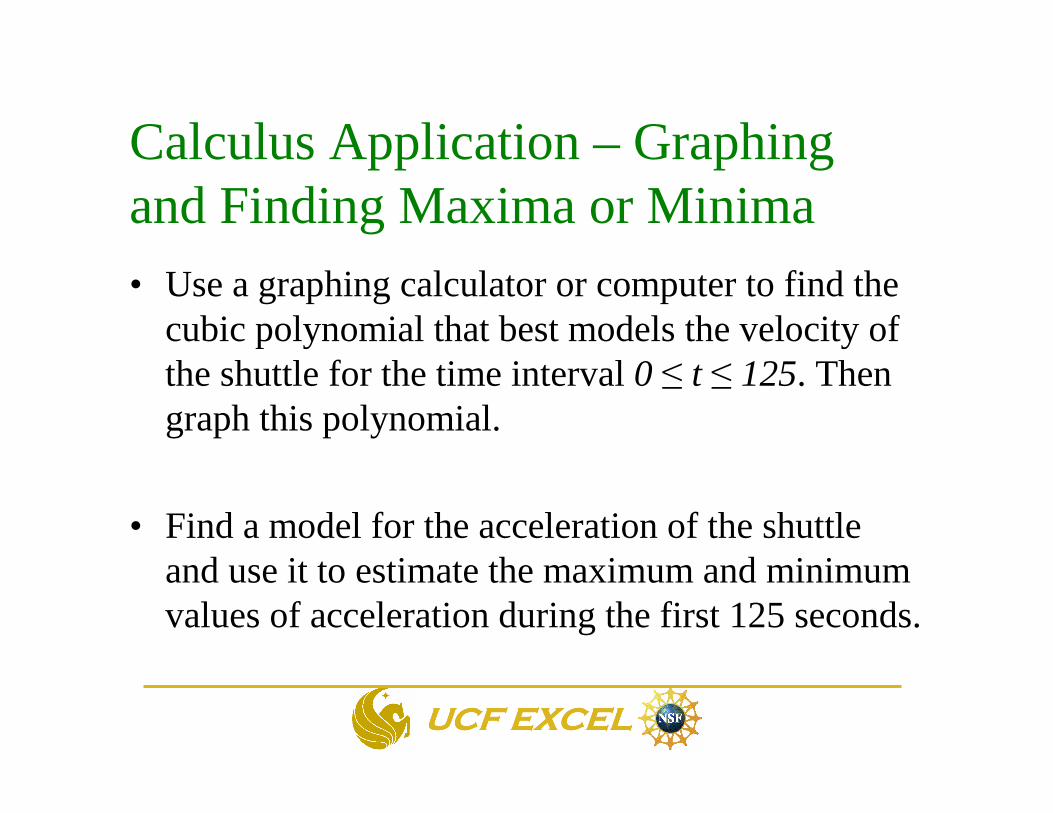
Calculus Application – Graphing and Finding Maxima or Minima• Use a graphing calculator or computer to find the

cubic polynomial that best models the velocity of the shuttle for the time interval 0 ≤ t ≤ 125. Then graph this polynomial.

• Find a model for the acceleration of the shuttle and use it to estimate the maximum and minimum values of acceleration during the first 125 seconds.


Strategy!

• Let us use a computer program (MS-EXCEL) to graph the variation of velocity with time for the first 125 seconds of flight after liftoff.

• The graph is first created as a scatter plot and then a trendline is added.

• The trendline menu allows for the selection of a polynomial fit and a cubic polynomial is picked as required in the problem description above.


Shuttle Velocity Profile

y = 0.0015x3 - 0.1155x2 + 24.982x - 21.269

-500

0

500

1000

1500

2000

2500

3000

3500

4000

4500

0 20 40 60 80 100 120 140

Time (s)

Vel

oci

ty (f

t/s)


Solution

• From the graph, the function y(x)or v(t) can be expressed as

• Acceleration is the derivative of velocity with time.

269.21982.241155.00015.0)( 23 −+−= ttttv

982.24231.00045.0)(

)( 2 +−== ttdt

tdvta


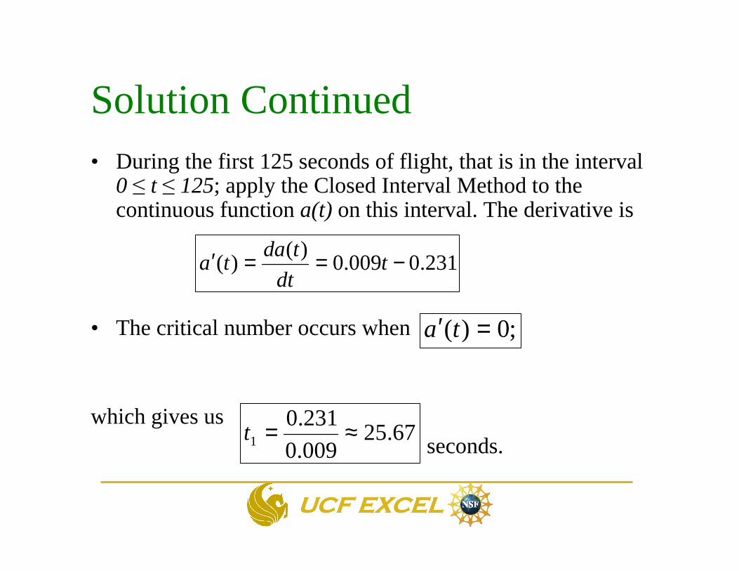
• During the first 125 seconds of flight, that is in the interval 0 ≤ t ≤ 125; apply the Closed Interval Method to the continuous function a(t) on this interval. The derivative is

• The critical number occurs when

which gives usseconds.

Solution Continued

231.0009.0)(

)( −==′ tdt

tdata

;0)( =′ ta

67.25009.0

231.01 ≈=t


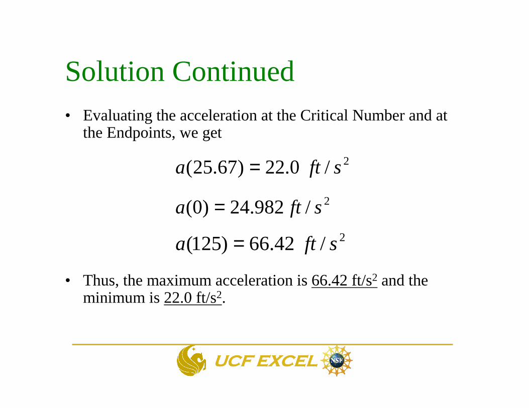
• Evaluating the acceleration at the Critical Number and at the Endpoints, we get

• Thus, the maximum acceleration is 66.42 ft/s2 and the minimum is 22.0 ft/s2.

Solution Continued

2/0.22)67.25( sfta =2/982.24)0( sfta =

2/42.66)125( sfta =


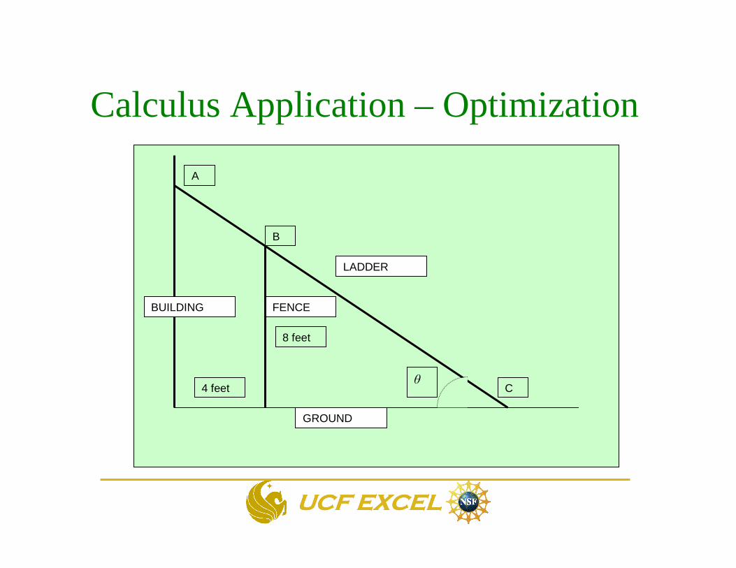
Calculus Application – Optimization

Section 4.7 #34:• A fence is 8 feet tall and runs parallel to

a tall building at a distance of 4 feet from the building.

• What is the length of the shortest ladder that will reach from the ground over the fence to the wall of the building?


Calculus Application – Optimization

θ

FENCE

B

A

C

8 feet

4 feet

LADDER

GROUND

BUILDING


Calculus Application – Strategy

• From the figure using trigonometry, the length of the ladder can be expressed as

L = AB + BC =

• Next, find the critical number for θ for which the length L of the ladder is minimum.

• Differentiating L with respect to θ and setting it equal to zero.

θθ cossin

DH +


Engineering Courses with Math

• Some future Engineering Courses at UCF that you may take are– EGN3310 – Engineering Mechanics – Statics

– EGN3321 – Engineering Mechanics – Dynamics

– EGN 3331 – Mechanics of Materials

– EML 3601 – Solid Mechanics

• and several of your engineering major courses


Use of Calculus in Engineering

• Real-world Engineering Applications that use Calculus Concepts such as Derivatives and Integrals

• Global and Local Extreme Values are often needed in optimization problems such as– Structural or Component Shape

– Optimal Transportation Systems

– Industrial Applications

– Optimal Biomedical Applications


Calculus Topics Covered

• Global and local extreme values

• Critical Number

• Closed Interval Method

• Optimization Problems using Application to Engineering Problems


Applications to Engineering

• Maximum Range of a projectile –(Mechanical and Aerospace engineering)

• Optimization of Dam location on a River (Civil engineering)

• Potential Energy and Stability of Equilibrium (Mechanical, Civil, Aerospace, Electrical Engineering)


Applications to Engineering

• Optimal Shape of an Irrigation Channel (Civil engineering)

• Overcoming Friction and other Forces to move an Object (Mechanical, Aerospace, Civil engineering)


Application to Projectile Dynamics

• Maximum Range for a Projectile

• May also be applied to Forward Pass in Football

• Goal 1: To find the Maximum Range Rof a projectile with Muzzle (Discharge) Velocity of v meters/sec

• Goal 2: Find Initial Angle of Elevation to achieve this range


Engineering Problem Solution

• Gather All Given Information

• Establish a Strategy for the Solution

• Collect the Tools (Concepts, Equations)

• Draw any Figures/Diagrams

• Solve the Equations

• Report the Answer

• Consider – Is the answer Realistic?


Given Information

• The Range R is a function of the muzzle velocity and initial angle of elevation :

• is the angle of elevation in radians and g is the acceleration due to gravity equal to 9.8 m/s2

θg

vR

θ2sin2

=


Strategy!• We need to find the maximum value of the range

Rwith respect to different angles of elevation.

• Differentiate Rwith respect to and set it to zero to find the global maxima. Note that in this case, v and g are constants.

• The end points for the interval for forward motion are 0≤ ≤ .θ

2

π

θ


Solution

g

vR

θ2sin2

= 0)2cos2(2

==g

v

d

dR θθ

02cos =θ

4,

2

1cos

01cos22cos 2

πθ

θ

θθ

=

=

=−=

or

As v and g are both non-zero,

Using trigonometric double angle formula:


And At the End PointsR(0) = 0R( ) = 0

Solution Continued

g

vR

2

)4

( =π

Evaluating the range at the Critical Value gives

2/π

Maximum range for the projectile is reached when or 45°

4

πθ =


Optimizing the Shape of Structures

• Relates to Fluid Mechanics and Hydraulics in Civil Engineering

• Civil Engineers have to design Hydraulic Systems at Optimal Locations along Rivers

• They also have to Optimize the Size of the Dam for Cost Constraints


Optimal Location of Dam

x

DAMSt. Johns River

City of Rock Springs

1020)( += xxD

)228(10)( 2 +−= xxxW

Depth of Water:

Width of River:


Example of a Dam on a River


Given Constraints and Questions• If the dam cannot be more than 310 feet wide and

130 feet above the riverbed, and the top of the dam must be 20 feet above the present river water surface, what is a range of locations that the dam can be placed (A)?

• What are the dimensions of the widest and narrowest dam(B) that can be constructed in accordance with the above constraints?

• If the cost is proportional to the product of the width and the height of the dam, where should the most economical dam be located (C)?


Strategy!

• Use the Closed Interval Method to find the widestand narrowestdam in the range of acceptable locations of the dam.

• Define the Cost Functionas proportional to the product of width and height

• Minimize Cost Function with respect to the location x measured from Rock Springs


Solution (A)

;51101020)( ≤⇒≤+= xxxD

91310)228(10)( 2 ≤≤−⇒≤+−= xxxxW

Based on the Specified Constraints

Width must be less than 310:

Depth must be less than 110

Range of locations for the Dam

50 ≤≤ x


Solution (B)

To obtain the widest (maximum W) and

narrowest (minimum W) for the dam, apply

the Closed Interval Method for the function

W(x) in the interval 50 ≤≤ x

)228(10)( 2 +−= xxxW

Differentiating: 08020)( =−= x

dx

xdW

4=xCritical Value:


Solution (B) Continued

220)0( =W70)5( =W

Corresponding width W(4)= 60 feetis the Minimum Width.Next, checking the endpoints of the interval, we obtain the following values:

feet and

Maximum Widthof the dam is 220 feetat Rock Spring (x = 0).

feet


Solution (C) Cost Minimization

)32(10302020)()( +=+=+= xxxDxH

)32)(228()( 2 ++−= xxxFxC

)6620132()( 23 ++−= xxxFxC

Height of Dam must be 20 feet HIGHERthan Depth of Water there -

Cost Function is Proportional to Product of H and W

Where F is a positive Constant; Simplifying -


Solution (C) Continued

3/10=x

0)( =

dx

xdC0)1)(103(2

)( =−−= xxFdx

xdC

3/10=x

.

To Find the Critical Number -

or

Solving for two values of x -or

Cheaper Dam is at Cost of Dam at this location = $62.30F

Checking Endpoints –at x=0, Cost = $66Fand at x = 5, Cost = $91F

MINIMUM COST = $62.30Fat 3/10=x


My Current Research Areas

• Permeable Concrete Pavements

• Soil Erosion and Sediment Control

• Slope Stability of Soil Structures and Landfills

• Modeling of Structures – Pile Foundations


Permeable Concrete Pavements


Optimization of Water Transport Channel

• Applies to Land Development and Surface Hydrological Engineering

• Such applications are common in Water and Geotechnical areas of Civil Engineering

• Part of the Overall Design of the Irrigation Channel – other areas Structural design, Fluid Flow Calculations and Location


Irrigation Water Transport Channel


Objective

h2h1 d

be1 e2

dd

Irrigation Channel

A trapezoidal channel of uniform depth d is shown below. To maintain a certain volume of flow in the channel, its cross-sectional area A is fixed at say 100 square feet. Minimize the amount of concretethat must be used to construct the lining of the channel.

is the angle of inclination of each side. The other relevant dimensions are labeled on the figure.

θ1θ

2θ


Strategy!

• Make Simplifying Assumptions (at this level) –

• Minimize the Length L of the Channel Perimeter excluding the Top (surface) Length

., 2121 eeeand ==== θθθ


Solution

21 hbhL ++=Based on Geometry:

θsin21

dhh ==

θtan

100100,

2

12100

d

de

dbor

edbdA

−=−=

+==

Since the Cross-sectional Area of the Channel must = 100 sq ft


Solution - Continued

θθ sin

2

tan

100 dd

dL +−=

Wetted length (Length in contact with water when full)

Minimizing L as a function of and d requires advancedmultivariable calculus. To simplify, let us make a DESIGN ASSUMPTION. Assume one of the two variables -

θ

3

πθ =



( ) dd

dfL 3100−==

.5984.73

10,

3

100,

03100)(

4

2

2

==

=

=+−=′= −

dor

dor

ddfdd

dL

Expression for L now is -

To get Global Minimum for L for

∞<< d0



0200

)(3

>=′′d

df in the interval ( )∞,0

Length of the Channel with d = 7.5984

322.26)5984.7( ≅f

is the Global Minimum

Since


Soil Erosion Test Laboratory


Minimizing Energy to Build Stable Systems

• Applies to both Mechanical and Civil Engineers

• Potential Energy is encountered in Mechanics and in Machine Design and Structural Analysis

• Minimizing Potential Energy maintains Equilibrium State and helps in Stability


Example - Pinned Machine Part


Given Information

Pinned Bars form the parts of a Machine

Held in place by a Spring

Each Bar weighs W and has a length of L

Spring is UNSTRETCHEDwhen and in equilibrium when

0=α°= 60α


Objective

• Find the value of the Spring Constant such that the system is in Equilibrium

• Determine if this Equilibrium Position is Stable or Unstable?


Strategy!

• Note that the “forces” that do the work to generate potential energy are – Weight of the Bars

– Force in the Spring pulling to the right

• Express Potential Energy U as a function of the angle and solve for k using α

0=αd

dU


SolutionSetting the Reference State or Datum at A –

Potential Energy = Sum of (Weight of each Bar times the Translations or movement of each Bar)


Solution - continuedDue to the two Bars – potential energy is

ααα sin)sin2

1()sin

2

1(1 WLLWLWU −=−+−=

Change in spring lengthor stretch of spring

αδ cos22 LL −=

Potential Energy due to Spring 22 )cos22(

2

1 αLLkU −=


Solution - continuedTotal Potential Energy becomes

21 UUU +=

22 )cos1(2sin αα −+−= kLWLU

or

When in Equilibrium state, Total U is in a MINIMUMstate with respect to the rotation from REST STATE

0=αd

dU


Solution - continuedDifferentiating and setting equal to 0 -

0)cos1(sin4cos 2 =−+−= αααα

kLWLd

dU

Given that the angle is °= 60α

Solving for k –

W

L

L

W

L

Wk

289.0

)60cos1(60sin4

60cos

)cos1(sin4

cos =−

=−

=αα

α


Stability Check

)60sin60cos60(cos460sin

)sincos(cos4sin

222

2222

2

+−+=

+−+=

kLWL

kLWLd

Ud ααααα

Second Derivative of Potential Energy is an INDICATOR ofStability of the System

If the Second Derivative of U is a POSITIVENumber, the System is STABLE!

As W, L and k are positive quantities, the Equilibrium Positionat is <STABLE>°= 60α


Application to Beams

• Design of Beams requires knowledge of forces inside the beam

• Two types – Shear and Bending Moment

• Design engineers PLOT the distribution along the beam axis

• Use Derivatives to determine Maximum and Minimum values and other parameters


Application of Calculus to Friction and Static Equilibrium Problem

• Friction is Important for Different Areas of Engineering – ME, AE, CE, and IE

• This example deals with a Concept you will see shortly in Engineering Mechanics Class

• Concepts Include – Free-body Diagrams, Friction, Newton’s Laws (3rd) and Equations of Equilibrium


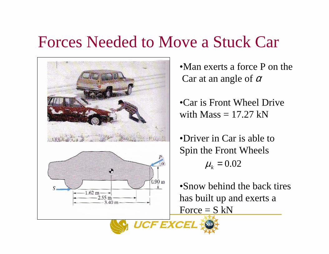
Forces Needed to Move a Stuck Car•Man exerts a force P on theCar at an angle of

•Car is Front Wheel Drivewith Mass = 17.27 kN

•Driver in Car is able to Spin the Front Wheels

•Snow behind the back tireshas built up and exerts a Force = S kN

α

02.0=kµ


Objective• Getting the Car UNSTUCK and moving

requires Overcoming a Resisting Force of S = 420 N

• What angle minimizes the force P needed to overcome the resistance due to the snow

α


Strategy!

• Draw Pictorial Representation of ALL forces on the Car – Free-Body Diagram (FBD)

• Apply Equations of Equilibrium to this FBD (will learn in PHY and use in EGN Classes)

• Express P as a function of angle of push

• Find the Global Minimum for P in the range

α

°<< 900 α


Free-body Diagram


Solution

• Equations of Equilibrium are applied to the FBD

• This implies the BALANCE of all the FORCES and MOMENTS (Rotations) on the System


Equations of Equilibrium

0)40.3(sin)90.0(cos)55.2()62.1(

0sin

0cos

=−++−=−−+

=−−

ααα

αµ

PPNW

PWNN

PNS

F

FR

Fk

)cos(1 α

µPSN

kF −=

αsinPWNN FR ++−=


Expression for Force P (angle)

0sin40.3cos90.0)cos(1

55.262.1 =−+−+− αααµ

PPPSWk

αd

dPDifferentiating, using the Chain Rule to find

and setting it equal to 0gives us the minimum value (critical) of α


Computations

0cos40.3sin40.3sin90.0cos90.0sincos55.2 =−−−+

+− ααα

ααα

αααµ

Pd

dPP

d

dPP

d

dP

k

0

cos55.2

sin40.3cos90.0

cos40.3sin90.055.2

=

−−

−

−−

=α

µαα

ααµ

α

k

k

P

d

dP


Minimum Value of Angle of Push

°=

−

=

54.1,

90.055.2

40.3tan

αµ

α

ork


The End

• You now know more about how Differential Calculus is used in Engineering!

• Good Luck!

• [email protected]

applications of calculus i - the excel program · applications of calculus i ... calculus concepts...

Documents