LAKE-GROUND WATER INTERACTION

at White Bear Lake, Minnesota

Report to the Legislative Committee

on Minnesota Resources

June 1998

Minnesota Department of Natural Resources

Waters

1

LCMR LAKE-GROUND WATER INTERACTION STUDY

at White Bear Lake, Minnesota TABLE OF CONTENTS PAGE ACKNOWLEDGMENTS 6 EXECUTIVE SUMMARY 7 SUMMARY: White Bear Lake HYDROLOGIC HISTORY: 11 General Geology/Hydrogeology Ground water Exchange Water balance Lake levels Precipitation Level Augmentation Lake Level Fluctuation Characteristics Runoff Surface outlet Evaporation Watershed Area Springs White Bear Lake TECHNICAL STUDY 29 Objectives Expanded Monitoring Climate Station Observation Wells Retrofitting White Bear Lake #3 Equipment/monitoring difficulties Outflow rating curve Mini Piezometer Outlet Rating Evaporation

2

LAKE/GROUND WATER MODELING 43 Ground Water modeling - general Modeling of Surface Water/Ground Water Interaction “MODFLOW” application to White Bear Lake "WATBUD" MODEL 52 Background Optimization/Calibration Philosophy Model Development Current Capabilities Variable SW/GW module Errors potential Future Development Document Model Application to Pickerel Lake APPLICATION OF "WATBUD" TO White Bear Lake 70 Lake Parameters Calibration GW Exchange Water Balance Future Levels CONCLUSIONS 82 BIBLIOGRAPHY 85

3

FIGURES/DRAWINGS 1. White Bear Lake Levels - Period of Record 2. Location Map 3. Geologic cross section 4. White Bear Lake-Obwell level Fluctuations 5. White Bear Lake-Obwell level Fluctuations 6. White Bear Lake Levels - Annual Precipitation 7. White Bear Lake Levels - 5-YR. Moving Average 8. Augmentation Well Geology and Construction 9. Lake level-Precipitation-Augmentation -Annual (Setterholm, 1993) 10. Lake level-Precipitation-Augmentation - monthly, 1924 thru 1934 11. Lake level-Precipitation-Augmentation - monthly, 1935 thru 1944 12. Lake level-Precipitation-Augmentation - monthly, 1945 thru 1954 13. Lake level-Precipitation-Augmentation - monthly, 1955 thru 1964 14. Lake level-Precipitation-Augmentation - monthly, 1965 thru 1974 15. Lake level-Precipitation-Augmentation - monthly, 1975 thru 1984 16. Lake level-Precipitation-Augmentation - monthly, 1985 thru 1996 17. Outlet Control History 18. Watershed - DNR Coates 19. Climate station data 20. Climate station data 21. Well locations 22. Continuous Lake/Ob Well levels 23. Recorded Precipitation - White Bear Lake levels 24. Recorded Precipitation - Hugo Obwell 25. Recorded Precipitation - Lake Jane Obwell 26. Outflow Rating Curve 27. Minipiezometer Locations 28. Minipiezometer Data 29. Evaporation - 1995 Daily 30. Evaporation - 1995 Daily 31. Evaporation - 1995 Cumulative 32. Evaporation - 1996 Daily 33. Evaporation - 1996 Cumulative 34. MODFLOW- upper layer 35. MODFLOW- lower layer 36. MODFLOW- LL heads w/o pumping 37. MODFLOW - LL heads w/ pumping 38. MODFLOW - LL heads w/o pumping- flow path 39. MODFLOW - LL heads w/ pumping- flow path 40. WATBUD - Hydrologic components 41. WATBUD - Areal components 42. WATBUD - Submodel Signatures

4

43. Pickerel Lake - Constant GWex 44. Pickerel Lake - Pumping Constant GWex 45. Pickerel Lake - Nonpumping Constant GWex 46. Pickerel Lake - Variable GWex 47. White Bear Lake - Area 48. White Bear Lake - Volume 49. White Bear Lake Future levels - Ave GWex PHOTOGRAPHS Climate Station at White Bear Lake Lake Jane observation well Goose Lake observation well Bellaire Beach observation well

5

ACKNOWLEDGMENTS Completion of this study was very much a team effort. The many involved were from Division of Waters staff, other agencies, local governments and local citizens. Division of Waters Staff having varying degrees of involvement in this LCMR project include John Linc Stine, Dave Ford, Laurel Reeves, Jim Zandlo, Greg Spoden, Jennie Leete, Sean Hunt, Jay Frischman, Chuck Revak, Brett Coleman, Fred Koestner, Julie Ekman and Corey Hanson. In addition Jerry Johnson’s AutoCAD expertise and Jim Zicopula’s desktop publishing expertise were essential in completing the project reports. The designated members of the White Bear Lake partnership and those participating in peer review meetings also provided valuable contributions towards project completion.

6

Executive Summary White Bear Lake has experienced wide fluctuations of water levels over the history of settlement and use of the lake and its shores. It has ranged in elevation from 919.89 feet (Ramsey County Datum) on February 6, 1991 to a high of 926.96 feet (Ramsey County Datum) on May 25, 1906. These wide fluctuations (exceeding seven feet) occur over a range of years and over changing annual climatic conditions (Figure 1).

During and after the recent drought period of 1988-1989, levels of White Bear Lake declined dramatically, approximately 4 feet over a three-year period. Afterward, even though the drought had dissipated and many area lakes had recovered to pre-drought levels, White Bear Lake remained well below long-term average levels. Residents, recreational users and local governments expressed concerns about this fact and asked the MN Department of Natural Resources (DNR) to investigate and report on the reasons for the continued below average lake levels. At the request and support of local communities and residents to investigate the sustained low levels, the Department sought funding for this project from the MN

7

Legislative Commission on Minnesota Resources (LCMR). LCMR asked whether the situation at White Bear Lake was unique to that particular lake. In responding, the DNR reported that White Bear Lake is not entirely unique; in fact, there are over 50 large developed lakes throughout Minnesota that are subject to wide long term level fluctuations similar to White Bear Lake. Such lakes do not have sufficient land drainage area (watershed) to sustain lake levels. White Bear Lake is one of these lakes. In further replying to the LCMR and the local community, DNR acknowledged that analyzing the causes and underlying relationships of such fluctuations would be very difficult. This lake/ground water interaction is a relatively underdeveloped branch of hydrologic analysis and modeling. Traditional forms of modeling lakes and watersheds are based on water budgets where ground water movement is generally thought to be much less significant than other factors such as precipitation, runoff and evaporation. In such situations, lake levels can be modeled by a basic inputs-and-outputs model like a checkbook balance. The rainfall and runoff are the water inputs - the outflow and evaporation are the basic water outputs. In lakes such as White Bear Lake, however, there is not enough inflow from precipitation and runoff to account for the changes in water levels. Therefore, a model was needed that also described the lake/ground water interaction. The LCMR concurred and in 1994 funded this project that is entitled, “Lake/Ground water Interactions at White Bear Lake”. LCMR funding ($175,000 over approximately three years) provided the DNR with the financial resources to accomplish these objectives. This report is the Department's final documentation of the project's results. The project was designed by the DNR with the assistance of local residents, technical peer advisers, and other units of government to enhance the technical analysis of the influence of ground water on Minnesota lakes in order to improve the understanding of lake level fluctuations and the underlying causes for such fluctuations. The project was also designed to build a technical base for making decisions about future actions that may affect water levels such as ground water pumping for municipal water supply, lake augmentation pumping, etc. The project had two basic objectives: 1. To expand and enhance an existing computer model (WATBUD, an abbreviation

for water budget), developed by the DNR in the mid-1980's, by adding a dynamic component for ground water exchange (water movement to or from the lake via ground water). The original version of WATBUD computes ground water exchange as an unchanging value in the water budget equation; this assumption is not valid at White Bear Lake. Because of the lengthy period of rainfall and water level data collected at White Bear Lake, the project also included

8

calibrating the modeled lake levels to actual experienced lake levels. This calibration would assist in determining the accuracy of the model as a predictive tool for future climate conditions, ground water pumping, etc.

2. To install necessary ground water observation wells and other scientific

equipment needed to provide accurate, continuous data on climate, lake levels, and ground water conditions for development and calibration of the WATBUD model. The additional equipment installation and the data collection efforts would allow DNR to determine how much information might be required to allow the model to be used for analysis of other similarly situated lakes across Minnesota.

The two primary benefits of the project to the citizens of Minnesota are: 1) the development of an enhanced computer model (WATBUD) to assist in answering difficult lake level and ground water level fluctuation problems for Minnesota lakes, and 2) additional observation well data for the benefit of computerized modeling of the Twin Cities regional ground water modeling efforts (underway by other agencies). During the course of the project, the DNR convened periodic meetings of interested residents, other units of government and technical experts. These meetings were held approximately twice per year and served to inform both the meeting attendees of the DNR's work on the project and the DNR of questions, comments and concerns of others. Semiannual status reports were prepared by the DNR and submitted to the LCMR and other interested individuals during the project. The following report is organized in several sections to describe the various project components including: ! description of the physical setting of White Bear Lake ! summary of earlier reports about White Bear Lake ! description of the technical details of the WATBUD computer model ! a comparison of the WATBUD model with respect to other available computer

simulation models that may be considered for analyzing lake and ground water relationships

! a discussion of the DNR's analyses and calibration efforts to test the potential

accuracy of the WATBUD model

9

As a result of this project, the DNR has developed a more useful technical analysis tool for use by other water resource professionals, units of government, lake associations, and individuals. The model allows for use of commonly available or attainable data, and it is available to anyone requesting it from the DNR. the model is written in a Windows 3.11 compatible format and contains an internal user help system similar to other Windows-based software. The following work plan products have been completed as a result of this project: ! Final report summarizing project and focusing on White Bear Lake water balance

characteristics. ! The completion and availability of “beta” version WATBUD computer model for

lake water balance computations. ! User’s manual describing basic model use. ! Detailed model documentation via software internal help files. ! Construction of 5 additional observation wells in the White Bear Lake area for

future monitoring needs. ! Retrofitted augmentation well to well code for future Mount Simon-Hinckley

monitoring needs. ! Construction of a steady state MODFLOW ground water model for White Bear

Lake covering the eastern Twin City metropolitan area. An abstract describing the WATBUD model and use was accepted and paper presented at the NALMS 1996 Annual Conference to be held in Minneapolis in November 1996. KEY CONCLUSIONS ! Historic level fluctuations have ranged as much as 7 feet. ! The watershed area is larger than previously documented. ! Augmentation has increased levels. ! Augmentation appears to increase water exchange to aquifers. ! Augmentation is not 100% efficient. ! Level increases due to augmentation are short-lived (less than a year). ! Lake fluctuations are strongly correlated to aquifer fluctuations. ! Reductions to the outlet control elevation have reduced peak lake levels.

10

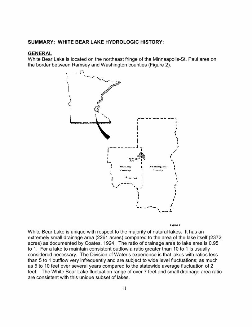
SUMMARY: WHITE BEAR LAKE HYDROLOGIC HISTORY: GENERAL White Bear Lake is located on the northeast fringe of the Minneapolis-St. Paul area on the border between Ramsey and Washington counties (Figure 2).

White Bear Lake is unique with respect to the majority of natural lakes. It has an extremely small drainage area (2261 acres) compared to the area of the lake itself (2372 acres) as documented by Coates, 1924. The ratio of drainage area to lake area is 0.95 to 1. For a lake to maintain consistent outflow a ratio greater than 10 to 1 is usually considered necessary. The Division of Water’s experience is that lakes with ratios less than 5 to 1 outflow very infrequently and are subject to wide level fluctuations; as much as 5 to 10 feet over several years compared to the statewide average fluctuation of 2 feet. The White Bear Lake fluctuation range of over 7 feet and small drainage area ratio are consistent with this unique subset of lakes.

11

GEOLOGY/HYDROGEOLOGY

Bedrock Geology White Bear Lake is underlain by St. Peter Sandstone and Prairie du Chien group bedrock units. The greatest part of the lake has St. Peter underneath it. The St. Peter Sandstone is a fine to medium grained quartz sandstone. In its lower zone, it is composed of mudstone, siltstone, and shale with interbedded coarse sandstone, which acts as a confining unit. The upper part of the Prairie du Chien Group is composed of thin-bedded dolostone with sandstone and chert. The Lower part is composed of thick-bedded dolostone. The St. Peter rests unconformably on the Prairie du Chien. Note: the Jordan Sandstone lies beneath the Prairie du Chien Group. It is a medium-grained friable quartz sandstone. It is in direct hydrologic contact with the basal Prairie du Chien. In effect, the two units act as a single aquifer. Depth to bedrock varies from less than 30 feet on the southwest shore to greater than 200 ft on the northeast shore. The majority of the lake area appears to have a thickness of surficial deposits between 50 and 150 feet thick.

Surficial Geology White Bear Lake is part of a chain of lakes that formed from blocks of ice lodging in bedrock valleys and the subsequent melting of the ice creating depressions in the landscape. On top of the bedrock units are several units of glacial origin covering the majority of the lake area. A deeply incised bedrock valley is found on the northeast end of the lake. (Figure 3)

12

The sequence of glacial deposits in the eastern portion of the lake from bottom to top are: olive brown glacial till deposits of pre-Wisconsin age; reddish-brown, sandy to loamy unsorted glacial till associated with the Superior Lobe; and, directly beneath the lake, sandy to gravely outwash associated with the Superior Lobe. The western portion of White Bear Lake is underlain, from bottom to top, by: meltwater stream deposits of medium to coarse grained sand associated with the Superior Lobe; loam textured till associated with the Grantsburg Sublobe with bands of Superior Lobe till; and, directly beneath the lake, sandy lake sediment consisting of fine to medium grained sand with silt and clay associated with the Grantsburg Sublobe. The western portion of White Bear Lake is on the edge of the southern extent of the Anoka Sand Plain that was created by outwash from the melting of the Grantsburg Sublobe of the Des Moines Lobe.

Hydrogeology The Prairie du Chien/Jordan formation are one of the two major aquifers in the Twin City area (the other is the Mount Simon). The St. Peter Sandstone also supplies water locally. Some units of the glacial material act as water table aquifers that interact with White Bear Lake. Potential yield from the St. Peter Sandstone is less than 250 gallons per minute (g.p.m.) and from the Prairie du Chien/Jordan is less than 1000 g.p.m. (1000-2000 g.p.m. at SE 1/4 of White Bear Lake)

The ground water flow direction in the water table aquifer is generally toward the west/northwest. The bedrock aquifers have higher heads at White Bear Lake than at the Mississippi River near St. Paul and their ground water flow direction is generally toward the southwest. Ground water Exchange The geology of the area, lake levels and ground water levels (heads) all affect the volume of lake-ground water exchange at any point of time. As lake and ground water levels change over time, the exchange volume also varies. The deepest part of White Bear extends to an approximate elevation of 840 ft. Observation wellheads in bedrock aquifers south and west of the lake vary from 860 to 912 ft and north of the lake from 928 to 947 ft. Comparisons of lake level graphs with ground water level graphs shows a strong correlation between the timing of highs and lows of lake levels and observation well levels (Figures 4 and 5). This is a strong indication the two are strongly hydraulically connected and therefore interact with one another Understanding the degree to which lake level fluctuations affect ground water level fluctuations and vice versa is extremely important in understanding the water balance of the lake.

13

14

15

WATER BALANCE The factors that drive the level fluctuations of White Bear Lake are the same as those that affect the levels of any other lake. They are the components of the hydrologic cycle: precipitation, runoff, surface outflow, evaporation and lake-ground water exchange. In the case of White Bear Lake another factor that has historically affected lake level fluctuations is pumped augmentation from ground water to the lake. The lake water balance equation can be used to mathematically express how the various components of the hydrologic cycle combine to affect lake levels over any time period. �L = P+RO-SO-E+GWex+PA �L = change in water level volume over period P = direct precipitation volume onto lake surface RO = runoff volume from drainage area SO = volume of outflow from surface outlet E = evaporation volume from lake surface GWex = volume of ground water exchange with lake [can be positive(+) or negative(-)] PA = volume of pumped augmentation (if any) Average Annual Water Balance Using data from generally available information sources, the average annual water balance for White Bear Lake (without accounting for augmentation and in equivalent inches over a 2400 acre lake) is: PRECIPITATION=30" 1961 to 1990 normal (NWS) RUNOFF=12.5" 1961 to 1990 normal (DNR/USGS) EVAPORATION=-36" Evaporation atlas (NOAA) To achieve “balance” the SW/GW exchange as the residual would be: GWex = -30"-12.5"+36" = -6.5 inches/year Using these data, White Bear Lake averages 6.5 inches of water exchange per year from the lake to ground water resources. If this value were positive it would indicate the opposite direction of net flow or ground water into the lake. The current area subject to runoff is 4995 acres as indicated on page 21.

16

Coates annual water balance - 1924 calendar year PRECIPITATION=25" RUNOFF=4.6" (Coates runoff area = 2261 acres) EVAPORATION=-29" LEVEL change = -6.6" GWex = -25 - 4.6 + 29 -6.6 = -7.2 inches/year DNR winter ground water exchange estimate (1993): GWex = - 5.7 inches per year LAKE LEVELS The systematic collection of White Bear Lake water levels by Ramsey County since the early 1920's and sporadic data dating back to 1901 (Figure 1) allows for a very complete picture of historic levels. The length and detail of this history are extremely important in helping to understand the significance various water balance parameters have in causing level fluctuations and also in assessing how much we don't yet understand about what drives level fluctuations at White Bear Lake. PRECIPITATION How much precipitation falls, how fast it falls and the area over which it falls are key factors that affect White Bear Lake water level fluctuations. That which falls directly on the lake immediately affects the level. Precipitation that falls on the lake's drainage area indirectly affects the levels through runoff, interflow (shallow subsurface flow) and ground water recharge. Precipitation that recharges ground water systems that affect the lake usually falls over a much greater area than the surficial drainage area. Precipitation records for Mpls-St. Paul (MSP) are available as far back as the early 1800's. However, precipitation can vary appreciably between the downtown areas and White Bear Lake and records at or very near the lake are only available since about 1960 . These more localized data are now available through volunteer monitoring networks where data acquisition and storage are coordinated through the University of Minnesota and the DNR State Climatology office. For this report, regional data are from the Minneapolis-St. Paul (MSP) airport, local data are from volunteer data collectors near the lake and site specific data are collected at the lake or within it’s watershed as part of this project. The closest available “local” data begins in the mid 1970's and has been included in the data set assembled for White Bear Lake. The site-specific data collection began in October 1994.

17

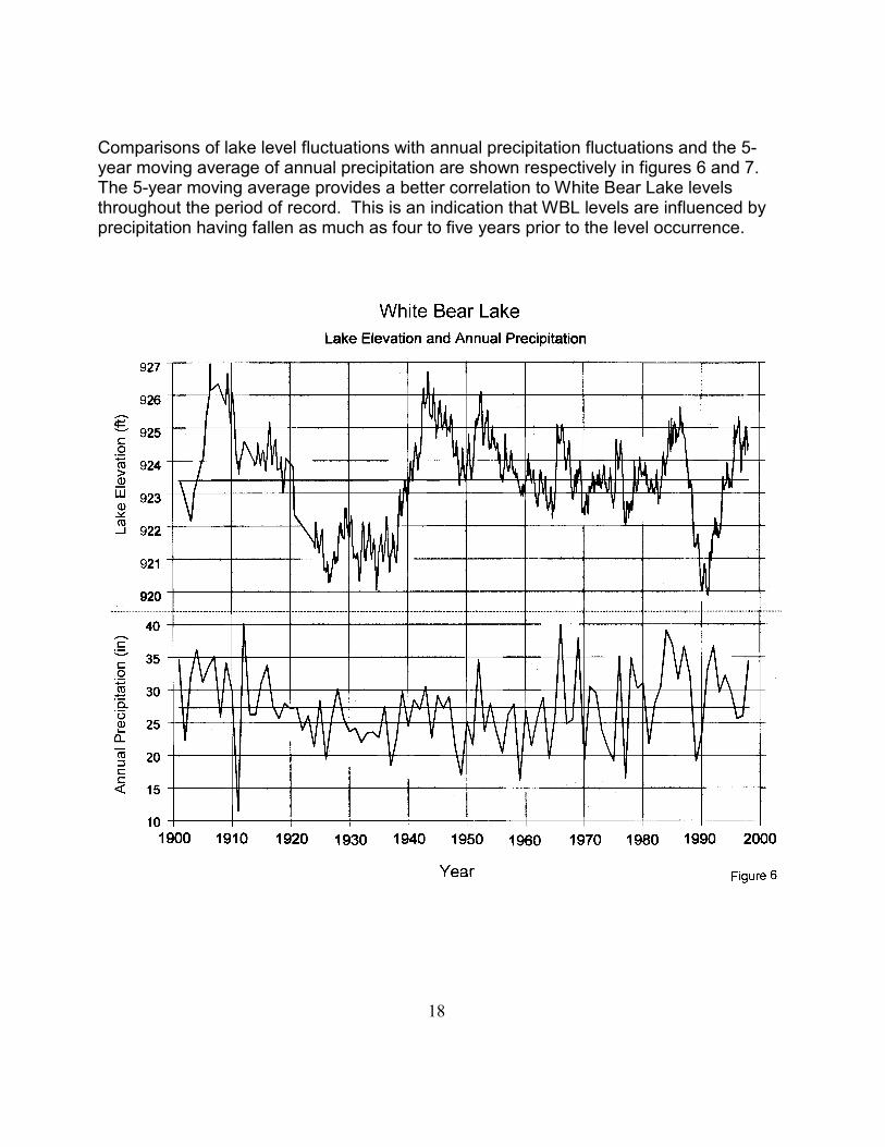
Comparisons of lake level fluctuations with annual precipitation fluctuations and the 5-year moving average of annual precipitation are shown respectively in figures 6 and 7. The 5-year moving average provides a better correlation to White Bear Lake levels throughout the period of record. This is an indication that WBL levels are influenced by precipitation having fallen as much as four to five years prior to the level occurrence.

18

LEVEL AUGMENTATION Lake level augmentation from ground water began by Ramsey County in the early 1900's and detailed records are available since 1924. Four lake level augmentation wells were installed at White Bear Lake. The locations of these wells are shown in figure 21. When all were in use, the maximum rate of augmentation was 5200 G.P.M. However, throughout any augmentation period, the rate varied significantly depending on the combination of wells and pumps used. Most periods of augmentation lasted few to as many 20 consecutive years and the rate has varied significantly throughout these periods. By documenting individual pump rates and on/off dates from Ramsey County White Bear Lake level charts the Division of Waters has developed a database of daily pumping rates beginning in 1924.

19

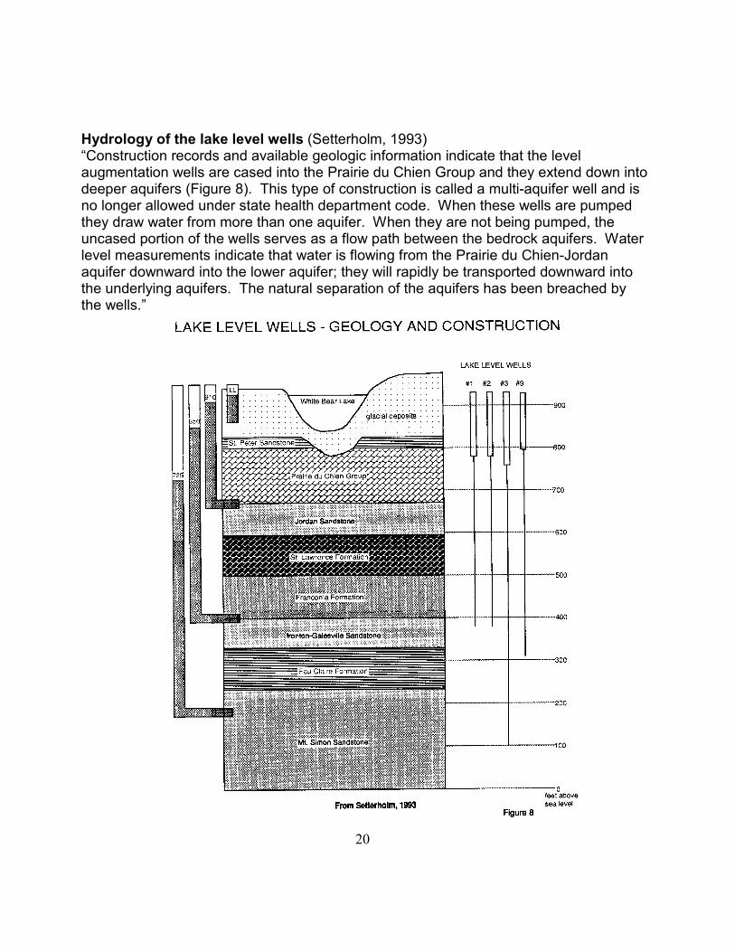
Hydrology of the lake level wells (Setterholm, 1993) “Construction records and available geologic information indicate that the level augmentation wells are cased into the Prairie du Chien Group and they extend down into deeper aquifers (Figure 8). This type of construction is called a multi-aquifer well and is no longer allowed under state health department code. When these wells are pumped they draw water from more than one aquifer. When they are not being pumped, the uncased portion of the wells serves as a flow path between the bedrock aquifers. Water level measurements indicate that water is flowing from the Prairie du Chien-Jordan aquifer downward into the lower aquifer; they will rapidly be transported downward into the underlying aquifers. The natural separation of the aquifers has been breached by the wells.”

20

Augmentation Summary No level augmentation occurred during the following years: 1943-1947, 1952-1953, 1957, 1962, 1966-1967, 1971-1976, 1978- present. Maximum pumped in any year: 2551 Million Gallons (MG) in 1932 = 7,825 acre-ft. = 3.56 ft. over 2200 acre lake Maximum pumped in any month: 250.0 MG in August, 1931 = 767.5 acre-ft. = 0.35 ft. over 2200 acre lake Maximum pumped in any Jan-Feb: 469.6 MG in 1932 = 1,441 acre-ft. = 0.66 ft. over 2200 acre lake (The lake level rose 0.67 ft and 0.24 ft of precipitation fell over period.) Total Pumped: 1924 thru 1977 = 45,480 MG = 58 feet over surface of lake (2400 acre lake) = average of 1.1 ft./yr (2400 acre lake)

21

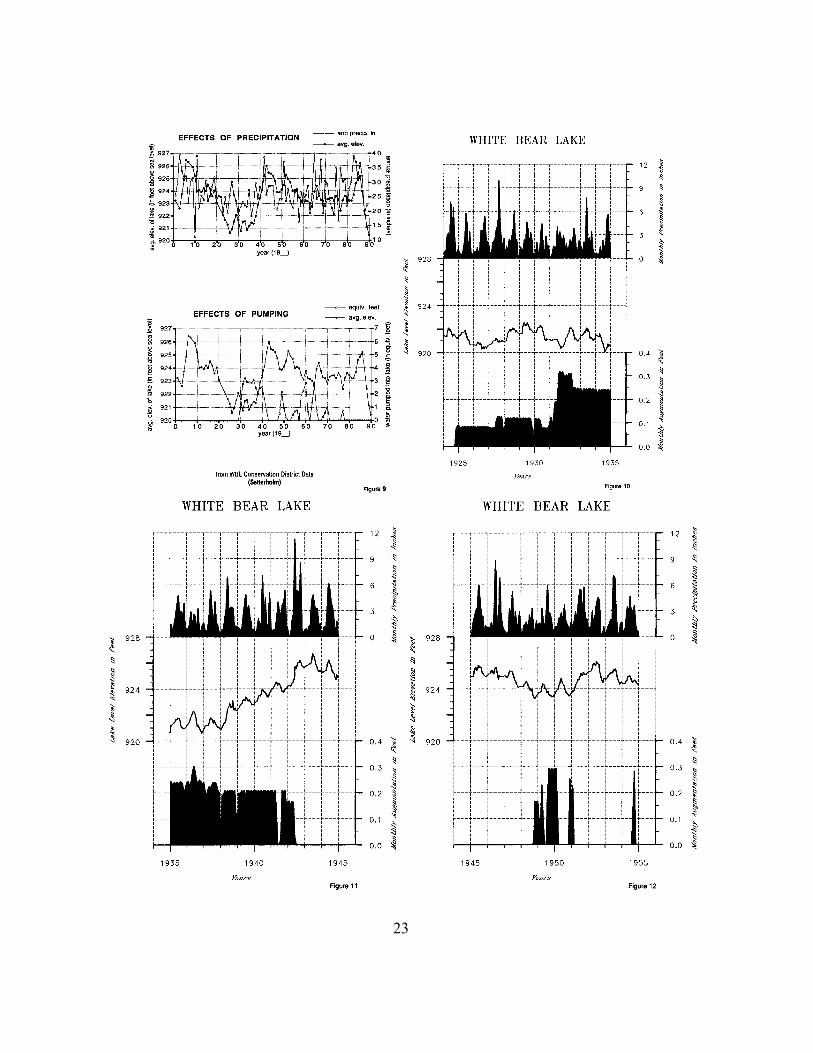
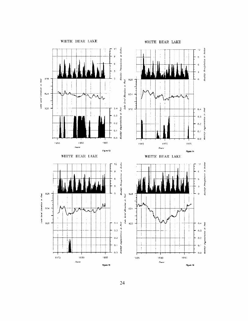
LAKE LEVEL FLUCTUATION CHARACTERISTICS Figures 9 through 16 show comparisons of lake levels, monthly precipitation and monthly pumped augmentation volume (equivalent feet over 2400 acre lake) for 10-year periods from 1924 to 1996 and are the basis for the following observations. During wet periods, summer lake level increases generally exceeded declines and during dry periods, summer declines generally exceeded increases. Years without augmentation show remarkably little winter fluctuation. This is in sharp contrast with summer levels that fluctuate significantly. Winters (Dec.-Feb.) during non-augmentation periods showed very little lake level fluctuation -- less than 0.2 feet over the 3-month period. During augmentation periods winter increases of over 0.2 feet occurred frequently. This is contrasted with maximum level declines of up to 1.0 foot during the summers of generally normal to above normal rainfall (1978-1986) and declines up to 2.0 feet during summers of less than normal precipitation (1987-1990). Winter levels during years with heavy winter augmentation often showed significant level increases of 0.5 to 1.0 feet. This occurred during all winters during the decade of the 30's with the maximum winter level increase occurring during the '31-'32 winter. Summer levels during periods of augmentation showed significant fluctuation. It appears from level graphs that during the early 80's (1983-1985) lake levels, absent augmentation, increased over winter periods indicating a net ground water flow to the lake. This is in contrast to most other non-augmentation years when level decline throughout winter periods is apparent. In late November of 1984 the lake rose 0.6 feet in two weeks. Levels then fell 0.6 feet in the subsequent two weeks. This unusual fluctuation likely was likely caused by some outlet obstruction and subsequent removal as no precipitation was recorded during that period.

22

23

24

RUNOFF Watershed topography, soils and land use, in addition to areal and temporal distribution of precipitation are key factors affecting runoff quantity. When streams or rivers feed a lake, the runoff flow can usually be measured. At White Bear Lake runoff is from the storm sewer system or overland flow and each is relatively difficult to measure directly. Because the area of the watershed is small compared to the area of the lake, this parameter is relatively small. For modeling purposes runoff is usually estimated as a mathematical function of precipitation and the lakes’ watershed characteristics. SURFACE OUTLET The current outlet of White Bear Lake functions infrequently and provides somewhat of a limit to high levels. The outlet consists of a channel and twin 30" arch culverts under the Ramsey County Beach parking lot. These culverts provide a control to outflow such that no water will flow out of the lake via the outlet channel when the lake level is below the upstream invert of these culverts. This outlet control is referred to as the "runout" and has been surveyed as part of this project to be elevation 924.3 feet above sea level, Ramsey County datum. On October 31,1906 the Ramsey County Board established the level of White Bear Lake to be 926.30 feet. This was described as “the upstream edge of sloping concrete slab in place immediately upstream of the three lines of 24" culverts”. This slab was breached in 1943 due to high water and the outlet control apparently reverted to the flowline of the culverts. As of 1981 the outlet control was described as the flowline of three lines of 30 inch diameter culverts, elevation = 925.5 feet. In the summer of 1982 Ramsey County reconstructed portions of the beach parking area that included replacing the three 24 inch culverts with the previously described twin 30-inch arch culverts. Figure 17 shows the outlet control elevation history compared to levels. The current outlet control elevation of 924.3 has reduced both the level and duration of WBL levels. Because the runout is currently 2 feet lower than existed prior to 1940, it is highly unlikely that the highest known level of 926.96 will ever again be reached. At times, a buildup of soil in the channel or debris at the culverts entrance has temporarily increased this elevation until the soil or debris is removed. A blockage of this nature or a more complete blockage of the outlet could result in artificially high levels.

25

Figure 17 EVAPORATION Variations in air temperature, water temperature, wind, humidity, and percent sunshine all affect how much evaporation will occur over any period. The inability to directly measure evaporation from a lake basin requires this element of the water balance equation to be estimated. Methods for estimating this parameter usually involve use of mathematical models incorporating one or more of these measurable components or adjusting data from an evaporation pan to compensate for differences in pan versus the lake. It is important to note that as the lake level changes so does the surface area of the lake subject to evaporation.

26

WATERSHED AREA In 1924 Coates documented the area of White Bear Lake to be 2372 acres, the basin area to be 4633 acres and the watershed area to be 2261 acres. Over the years, many have used these values to identify the watershed to lake area of 0.95 to 1. To verify or update these values for use in water balance simulation, existing DNR major and minor watershed maps and storm drainage maps from local governmental units were examined and documented. In addition field examinations were completed to verify areas of question. These efforts resulted in a basin area of 7,526 acres and a lake area (USGS quadrangle) of 2,531 acres. Using a consistent naming convention as by Coates results in a watershed of 4995 acres and a watershed to lake ratio of 1.97 to 1. Small noncontributing areas may exist in this delineation. In addition, the contributing watershed of most lakes can vary as climate regimes vary from wet to dry. Areas that are noncontributing during dry periods can fill during wet periods and the resulting outflow then contributes to the lakes water balance. The apparent increase in drainage area, between Coates and DNR delineations, is attributed to existing connections of wetlands by culverts and surface drainage that previously were separated and to existing storm sewer projects. See Figure 18 for a comparison of the Coates and the current DNR delineations.

27

SPRINGS Persons familiar with White Bear Lake often cite the existence of springs. These are described as areas of exceptionally cool water pockets noted when swimming. This is a phenomenon noticed on many lakes and is consistent with general understanding of the ground water exchange (GWex) component of a lakes water balance. In most lakes there are areas of ground water inflow and of ground water outflow. It is the sum of all inflow and outflow that is represented as the net GWex. Springs are localized areas of concentrated ground water inflow.

28

White Bear Lake TECHNICAL STUDY Objectives The technical study’s objective is to quantify the dynamic relationship of surface and ground water interaction at White Bear Lake. Examination of existing surface and ground water data indicate the timing of lake level fluctuations closely correspond to the timing of ground water level fluctuations (Figures 4 and 5). This suggests a very strong ground water influence on lake levels. It appears that surficial lake level change factors such as precipitation, runoff, evaporation and artificial augmentation (from any source) affect levels incrementally by relatively small amounts and the duration of this affect is short lived. If the amount and duration of these affects are quantified, the "efficiency" of level augmentation can be assessed in the short and long term and ultimately may be used to better balance or compare alternative solutions to identified lake needs. Detailed surface water/ ground water interaction questions to be explored through intensified monitoring and additional analysis including use of WATBUD and ground water modeling include: ! Detailed timing of lake and obwell fluctuations. ! Effect of augmentation and duration of this effect ! Expected level range and duration w/o augmentation ! Effect of high volume appropriators on levels ! Significance of site-specific data compared to local and regional data. ! Verify operation of WATBUD sub-model results with project site-specific data.

29

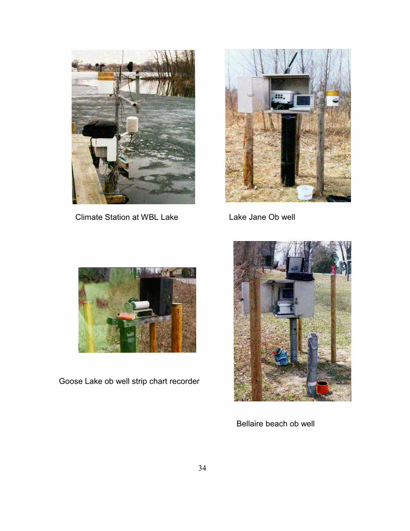
Expanded Monitoring The expanded monitoring was designed to provide site specific data for comparison with more readily available local and regional data, to better quantify the White Bear lake/ground water exchange (GWex) and to allow insight as to advantages and need of site specific data for analyses. The principal components of the intensified monitoring included deploying and maintaining continuous recording electronic data collection equipment at the lake and key observation wells in addition to constructing new observation wells for the project and future monitoring needs. By continuously recording lake level and nearby well level data as part of the White Bear Lake project, transients in water balance components can be analyzed in detail. This information would be useful in deducing the effectiveness and duration of past augmentation and in future level management decisions. The most notable hydrologic event of the monitoring period was 4.25 inches of rainfall over July 14 and 15, 1995. This resulted in a 6.0-inch lake level rise from July 14 to 16. Climate Station The climate station was setup on a private dock in the southwest corner of the lake on September 23, 1994. Parameters monitored by the station include air temperature, water temperature, lake level, precipitation, solar radiation, relative humidity, wind speed, and wind direction. Each parameter is stored on an hourly and daily basis and downloaded and processed weekly. Average daily data collected at the climate station are shown on figures 19 and 20. The climate station equipment is on loan from the Division of Waters Climatology office for the duration of the project.

30

Observation Wells The DNR-Division of Waters maintains a statewide network of water level observation wells some of which are in the vicinity of White Bear Lake. However, prior to this project only one, at the White Bear Lake Town Hall, was within close proximity the lake. To provide a better description of ground water levels in the vicinity additional wells were sited and constructed. These wells would be used in the short term to provide detailed data for the White Bear Lake technical study and in the long term as additional locations for the statewide observation well network. The locations of additional wells were chosen to fill gaps in the existing network in the area and to provide data specific to the lake. Initially, locations were sought for three wells within a few hundred feet of the lake. Other wells were to be drilled farther away in order to provide a comparison with the White Bear Lake wells. Continuous recording electronic data recorders were installed at each well to provide detailed level data. Prairie du Chien/Jordan aquifer wells were drilled at Bellaire Beach, which is north of Hugo along Hwy. 61 – at Withrow School and at Lake Jane. An additional sight was selected at Mahtomedi Beach, but access permission could not be obtained due to a conflict with proposed construction. To compensate, another location further north was selected, however, the process of obtaining access permission was so protracted that the well was not drilled because not enough data could be obtained from it to enhance this project. A water table well also was drilled adjacent to the Bellaire Beach well to assist in comparison of the lake levels and the deeper aquifer’s level.

31

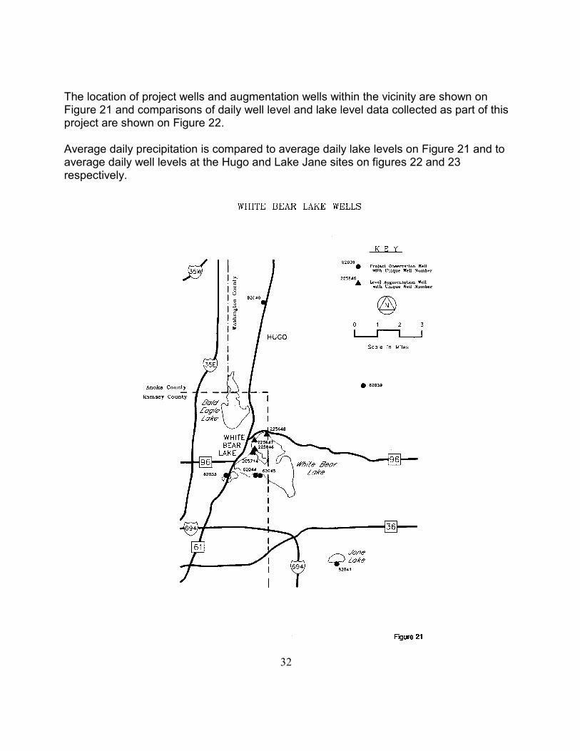
The location of project wells and augmentation wells within the vicinity are shown on Figure 21 and comparisons of daily well level and lake level data collected as part of this project are shown on Figure 22. Average daily precipitation is compared to average daily lake levels on Figure 21 and to average daily well levels at the Hugo and Lake Jane sites on figures 22 and 23 respectively.

32

33

Climate Station at WBL Lake

Goose Lake ob well strip chart recorder

34

Lake Jane Ob well

Bellaire beach ob well

Well Location/ Data Recorder Type

Well ID

T

R

S

Date Monitor-ing Started

Type of Data Collected

Bellaire-deep / CR10

62044 30N 22W 24 3/18/95 Air Temperature (F) Well Water Elevations (ft) Air Pressure (mbar)

Bellaire-shallow / CR10

62045 30N 22W 24 3/18/95 Air Temperature (F) Well Water Elevations (ft) Air Pressure (mbar)

Hugo / BDR 82040 31N 21W 8 1/6/95 Well Water Elevations (ft) Precipitation (in)

Lake Jane / CR10

82041 29N 21W 10 5/25/95 Air Temperature (F) Well Water Elevations (ft) Precipitation (in) Lake Elevation (ft)

Withrow / BDR 82039 31N 21W 36 12/19/94 Air Temperature (F) Well Water Elevation (ft)

White Bear Lake Town Hall / Stevens Chart Recorder

62038 30N 22W 23 8/8/94 Well Water Elevation (ft)

Weather Station / CR10

30N 22W 23 10/15/94 Mean Air Temperature (C & F) Vapor Pressure (kPa) Solar Radiation (langleys/days) Mean Wind Direction (Degrees from N) Wind Speed (m/s) Precipitation (in) Water Temperature (F) Lake Elevation (ft)

35

Retrofitting Ramsey County Well #3 One of the four wells used for augmentation of the lake (Figure 21), one was finished in the Mt. Simon Aquifer, the deepest aquifer actively used for water supply in the Twin Cities. All four wells are uncased allowing movement of water between aquifers. This type of construction is no longer allowed under the Water Well Construction Code and these wells could not be reactivated for any purpose without reconstruction. The statewide observation well network has very few Mt. Simon observation wells in the Twin Cities area due to the high cost of drilling such deep wells, often 800' - 1,000' deep. As demand and supply and water use patterns change, this aquifer is expected to face increased use pressure. Therefore, the possible retrofitting of Ramsey County Well #3 (#225647) was included as an option of this project. Ramsey County has made several attempts to gain knowledge of the well’s construction as a preliminary to sealing the well. They found that the well appears to have a strong bend (often deep wells are not straight caused when the drill bit is deflected by a particularly hard layer of rock). In addition a piece of pipe thought to be 20’ in length was obstructing the well at this bend although there was scant mention of this pipe in any of the 1926 construction or subsequent repair records of the well. As a follow-up of the County’s efforts, an attempt was made to place a video camera down the hole by threading it into the obstructing pipe. This effort failed. Consequently, 4" steel casing was passed through the 10" pipe. At that time a video camera was lowered to the bottom of the well at about 790' and a gamma log also was taken to verify the stratigraphy. This investigation showed that the obstruction thought to be 20' of 10" pipe was in fact 200' of 12" pipe. In order to reconstruct this well, the 4" casing was removed, the 12" pipe perforated to allow grout to fill behind it, the 4" pipe replaced and extended below the top of the Mt. Simon aquifer and the casing grouted. An extraordinary amount of grout was required indicating that the 12" pipe may have been placed to stop the sloughing of a soft formation. Unfortunately, the circulation of the grout was obstructed and the 4" casing was partially filled with grout. The well remains obstructed pending additional work. In addition, during the course of obtaining access permission, the ownership of the property was found to be clouded. The additional work has been delayed pending clarification of the property’s ownership and funding for the additional work. However, much of the work performed would have been required even if the well was to be sealed and the well no longer is allowing movement between aquifers. It is anticipated that both of these problems will be surmounted and the well added to the Observation Well Network within a year. Data from this well will add significantly to the long-term management of the region’s water supply.

36

Equipment/Monitoring Difficulties The availability of electronic data collection and monitoring equipment has substantially improved monitoring and analysis efficiency however, while more dependable than mechanical equipment, problems still occur as outlined at the sites below. All equipment was checked and data downloaded on a weekly basis to eliminate long data gaps resulting from malfunctioning equipment. Bellaire-deep well (#62044) The pressure transducer failed. It was replaced and the data was adjusted to show the actual well water elevations. Lake Jane well (#82041) Vandals cut the cable from the data collector to the pressure transducer, therefore continuous elevation data at Lake Jane was only collected from 6/9/95 to 6/28/95. No replacement of the cable was made. Withrow well (#82039) Power was lost to the data recorder because the batteries dropped below the low voltage threshold. The batteries were replaced and data during the time of the power failure was lost. White Bear Lake Town Hall well (#62038) This well is affected by nearby ground water pumping. White Bear Lake weather station 1) Sensor signal drift occurred in the lake level pressure transducer. The pressure transducer was recalibrated and data during the time of the drift was adjusted using staff gage readings taken during weekly equipment servicing. 2) The lake temperature probe data began to provide erroneous data indicating nearly complete failure, so a replacement temperature probe was installed. 3) During the late spring of 1996 the tipping bucket precipitation gage ceased recording all but major rainfall events. The gage was replaced. Hugo or Jane site precipitation will be used for missing period.

37

Outflow Rating Curve Outflow for various lake levels had been previously been computed by DNR using a computer program "HYDRP" that uses standard culvert hydraulic relationships. Field surveys and site drawings were used to further fine-tune the outlet outflow computer model. The occurrence of levels high enough to produce outflow allowed outlet flow measurements to be made. These outflow data were also used to further fine-tune the outflow rating relationship. (Figure 26)

Mini piezometer A mini-piezometer is a tool used to identify the difference in head or pressure between saturated lake bed sediments and the lake itself. If the head is higher in the sediments than the lake, the GWex flow direction is toward the lake and if higher in the lake than sediments it is out of the lake into the lake bed. Measurements were made on six days throughout the study to identify directional characteristics of GWex. Locations of measurements taken are shown in Figure 27 and data collected are summarized in figure 28.

38

39

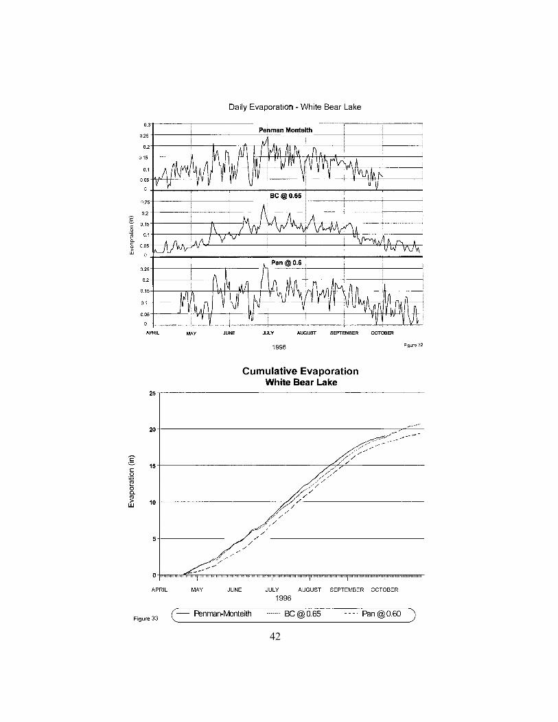
Evaporation Past Division of Waters studies have shown the Blaney Criddle model to provide good estimates of seasonal and annual mine pit evaporation. Climate data from the White Bear Lake weather station for summer 1995 were used in Penman-Monteith evaporation model to provide additional evaluation of the appropriateness of the Blaney Criddle model for use within WATBUD. A comparison of daily pan, Penman-Monteith and Blaney Criddle evaporation estimates are shown for October 1995 on figure 29 and for the 1995 open water period on figure 30. This comparison shows the Blaney Criddle daily estimate with an adjustment of 0.65 does not simulate the day-to-day variation in evaporation as well as the more data intensive Penman-Monteith estimate or the adjusted pan data. A comparison of cumulative variation in Figure 31, however shows the adjusted Blaney Criddle estimate provides similar season long estimates for the 1995 open water season as adjusted pan or Penman-Monteith method. Similar comparisons for 1996 are shown in Figures 32 and 33.

40

41

42

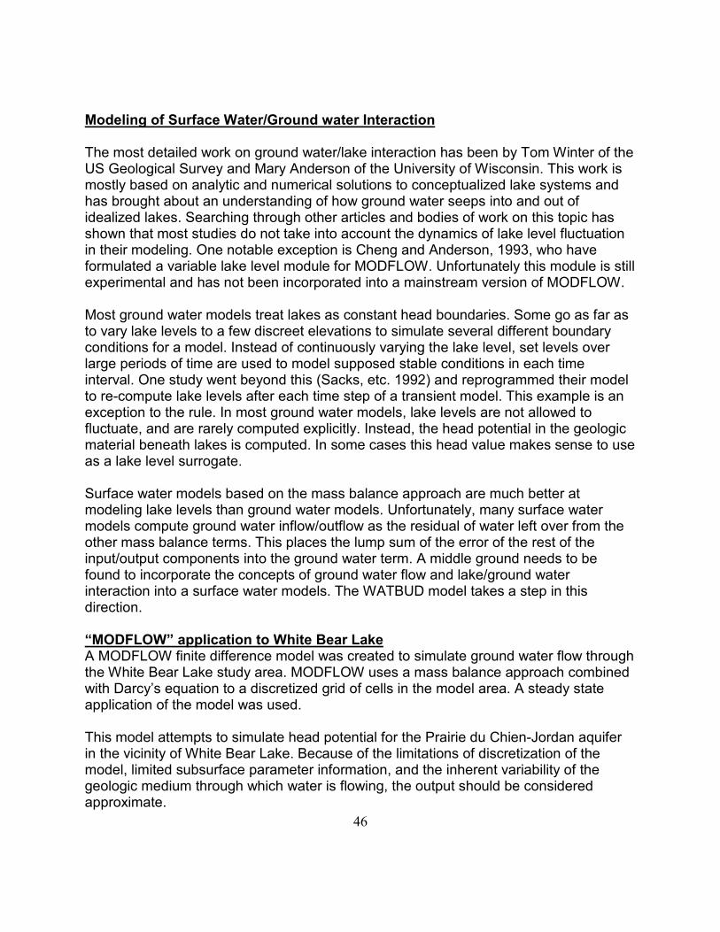
LAKE/GROUND WATER MODELING General Ground water modeling refers to the construction and operation of a model that can mimic the actual behavior of ground water in an aquifer system. There are several kinds of ground water models: physical (most physical models look like ant farms packed with layers of sand and clay), electrical analog, and mathematical. Physical models are scale models of a ground water system, typically built in aquariums or narrow Plexiglas 'ant farms' of sand, gravel, and clay or other porous materials. They directly try to mimic a natural flow system or a conceptualized system using a physical scale model. These are used mostly for demonstration purposes. Electrical analog models use the flow of electricity through a conductor as an analogy for water flowing through porous media to simulate ground water movement through an aquifer. The aquifer characteristics are scaled into the model by using resistors to represent the transmission of water and capacitors to represent the storage of water. When the model is finished, current represents the flow of water and voltage represents the hydraulic head (which can be understood as the water level in wells which penetrate the aquifer). Electrical analog models are rarely built today because other models are easier to work with. Mathematical models use a set of equations and assumptions chosen to represent to ground water system. Computer programs then solve these sets of equations. Mathematical models have replaced other types of models as the speed of computers has increased and the cost of computers has decreased. Mathematical models are derived from the physical laws that govern the situation (for example: conservation of mass, conservation of momentum, and Darcy's equation) with simplifying assumptions about the aquifer and about the edges of the modeled area. Analytical models can be used to solve very simple problems (for example, the aquifer can be assumed to be the same in every direction and only one value for each parameter is needed). Equations are set up which represent the system variables (for example hydraulic head) over the domain of the model. The resulting analytical model of ground water flow will be a set of partial differential equations that can be solved directly using calculus.

43

Graphical solution of some of the less complicated flow equations is possible. For example, flow nets combine lines that describe flow paths and lines that represent equal hydraulic head to provide a visualization of the ground water flow field. Once constructed, a flow net can be used for prediction of flow directions and amounts.

It is clear that many real world problems are not simple enough to be accurately assessed with analytical or graphical models. Where enough is known about a hydrogeologic problem to be able to characterize the system with variable aquifer parameters and detailed boundary conditions, the ground water flow equations cannot be directly solved with calculus; rather they must be approximated by systems of algebraic equations. Ground water models using this technique are termed numerical models. Calculations must be carried out repeatedly over the entire system of equations until a solution is reached. The process is repeated every time a change in any of the model data is made. The most commonly used numeric models fall into three categories: finite difference, finite element, and analytic element methods. Finite difference method The finite difference method superimposes a grid system over the study area. The method has developed to the point where the grid need not be regular. A finer mesh can be located over the area of greatest concern so that more detail can be obtained. Within each cell or aquifer segment there is a node point at which the equations are solved. The inputs and outputs of a model are considered to be uniform inside each individual cell, regardless of cell size. All water levels are calculated at the node and applied over the whole cell. To avoid a 'stair-step' effect in water levels, areas of concern should have finer meshes. The solution of the finite difference model is an iterative process. A first approximation of the head at each of the nodes is the starting point. The computer recalculates heads at each node (some nodes may have fixed heads as part of the boundary conditions), based on the heads of adjacent nodes, until the changes between successive recalculations is less than the predetermined error limit. The Modular Three-Dimensional Finite-Difference Ground-Water Flow Model (MODFLOW) developed by the U.S. Geological Survey is the most widely used finite difference model (McDonald and Harbaugh, 1988). Finite element method The finite element method divides the aquifer into polygonal elements (often triangular) by connecting irregularly placed nodes into a mesh where each element has multiple nodes. This discretization allows more accurate representation of irregular areas than does the finite difference model, even though the finite element model will usually have fewer nodes. Values of system variables are interpolated over the element by basis functions. The basis functions are specified in terms of the node coordinates and the results are combined into an integral system that is then approximated using finite difference techniques.

44

Analytic element method If you divide any ground water system into small enough pieces, you reach a point where the pieces are internally simple enough that analytical solutions can be used. Relatively uniform portions of the aquifer can be turned into model elements and because there are no restrictions on element size or shape, the model can be built with exactly the level of detail needed to meet the modeling requirements with no excess elements. The text on ground water model types was adapted from Leete, 1996.

45

Modeling of Surface Water/Ground water Interaction The most detailed work on ground water/lake interaction has been by Tom Winter of the US Geological Survey and Mary Anderson of the University of Wisconsin. This work is mostly based on analytic and numerical solutions to conceptualized lake systems and has brought about an understanding of how ground water seeps into and out of idealized lakes. Searching through other articles and bodies of work on this topic has shown that most studies do not take into account the dynamics of lake level fluctuation in their modeling. One notable exception is Cheng and Anderson, 1993, who have formulated a variable lake level module for MODFLOW. Unfortunately this module is still experimental and has not been incorporated into a mainstream version of MODFLOW. Most ground water models treat lakes as constant head boundaries. Some go as far as to vary lake levels to a few discreet elevations to simulate several different boundary conditions for a model. Instead of continuously varying the lake level, set levels over large periods of time are used to model supposed stable conditions in each time interval. One study went beyond this (Sacks, etc. 1992) and reprogrammed their model to re-compute lake levels after each time step of a transient model. This example is an exception to the rule. In most ground water models, lake levels are not allowed to fluctuate, and are rarely computed explicitly. Instead, the head potential in the geologic material beneath lakes is computed. In some cases this head value makes sense to use as a lake level surrogate. Surface water models based on the mass balance approach are much better at modeling lake levels than ground water models. Unfortunately, many surface water models compute ground water inflow/outflow as the residual of water left over from the other mass balance terms. This places the lump sum of the error of the rest of the input/output components into the ground water term. A middle ground needs to be found to incorporate the concepts of ground water flow and lake/ground water interaction into a surface water models. The WATBUD model takes a step in this direction. “MODFLOW” application to White Bear Lake A MODFLOW finite difference model was created to simulate ground water flow through the White Bear Lake study area. MODFLOW uses a mass balance approach combined with Darcy’s equation to a discretized grid of cells in the model area. A steady state application of the model was used. This model attempts to simulate head potential for the Prairie du Chien-Jordan aquifer in the vicinity of White Bear Lake. Because of the limitations of discretization of the model, limited subsurface parameter information, and the inherent variability of the geologic medium through which water is flowing, the output should be considered approximate.

46

The modeled area included all of Washington and Ramsey Counties, the southern 2/3 of Anoka County and a small portion of Hennepin County. The northern boundary is the top of Township 32 (also the northern end of Washington Co.) from the St. Croix to the Rum Rivers. The Rum and the Mississippi Rivers form the western and southern boundaries to Prescott, WI. The eastern boundary is formed by the St. Croix River. The model consists of two layers (39 rows by 32 columns) to roughly correspond to the Prairie du Chien-Jordan aquifer in the lower layer and the St. Peter and Drift/Till aquifers in the upper layer. Cell sizes are mostly one mile on a side with sides becoming 2 miles long near the periphery of the model area. Cell size in the vicinity of White Bear Lake is ½ mile on a side. The cells along the Mississippi River from Minneapolis to Prescott, WI and along the St. Croix River were modeled as constant heads in the lower layer. The Rum and the Mississippi Rivers north of Minneapolis were modeled as constant heads in the upper layer. Large lakes including White Bear Lake, Bald Eagle Lake, Forest Lake, Big Marine Lake, Lake Phalen, Pleasant Lake, and lakes in the Lino Lakes area were modeled as constant heads in the upper layer. The upper layer has a no flow boundary along the northern end of the model. The northern extent of the Prairie du Chein-Jordan aquifer is used as the northern model boundary in the lower layer. Four re-injection wells in the center of the northern end of Washington County were used to simulate flow from the outwash sands of the Anoka Sand Plain to the Prairie du Chein-Jordan system in the lower layer. Figures 34 and 35 show the upper and lower layer grid configurations. U.S. Geological Survey Water Resources Investigations Report 90-4001 (Schoenberg, 1990), which reported on a finite difference ground water flow model in the Twin Cities area, was used to help construct many of the initial hydrologic input parameters. In addition, published values for hydraulic conductivity and their ranges were consulted for starting values (Kanevetsky and Walton, 1978 and Lindgren, 1990). Interpreted lithologic well logs contributed to understanding the hydrogeologic system.

47

Model Calibration Model parameters were initially input as uniform values across the model domain. Values were modified from the starting conditions and tested for goodness of fit by comparing output results to published hydrogeology maps and observation well data. Values that produced a better fit and were within acceptable ranges were used. Next, hydraulic conductivity, storage coefficients, and recharge were varied to better represent the modeled areas. The configuration and injection rate of the northern wells were varied to produce the best output configuration. The simulation with pumping wells matched the observations wells most closely. The Hugo well had the greatest discrepancy. This may be due to its proximity to the model edge where conditions are generally not as well simulated compared to the model center. MODFLOW Modeling Results Water appropriation data for high capacity pumping wells completed in the Prairie du Chien-Jordan aquifer extracting on average greater than 10 million gallons/year were evaluated. Wells were simulated in MODFLOW using the WELL package. In MODFLOW multiple wells inside a cell are grouped together to extract water out of the

48

cell as if there were only one well. 33 cells had at least one high capacity well in the six townships surrounding White Bear Lake (T29R21, T29R22, T30R21, T30R22, T31R21, and T31R22).

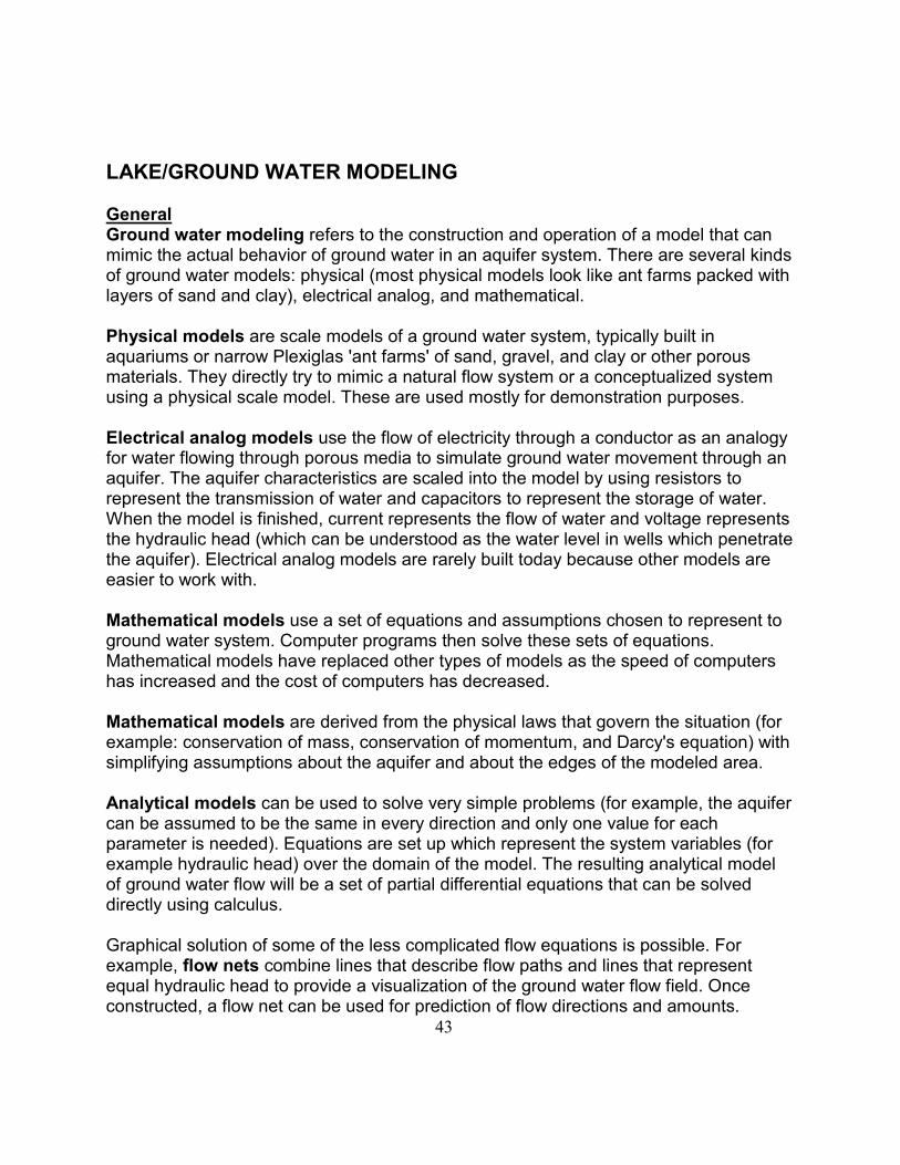
Running the model with and without the high capacity pumping wells produced changes in the head potential surface configuration of the layer representing the Prairie du Chien-Jordan aquifer. The steady state configuration without pumping wells shows heads ranging from 940 ft to 930 ft elevation in the White Bear Lake area (figure 36). With the pumping wells the head configuration ranges from 925 ft to 900 ft elevation over the same area (figure 37). The simulation with pumping wells is more realistic for modern day conditions than without pumping wells. The simulated higher heads without pumping indicates the potential exists for higher head levels in the aquifer directly below the lake. These higher levels would increase the upward water flow toward the lake. This would likely increase the moderating effect that the ground water connection has on the lake level.

The modeling of flow pathlines with and without pumping wells shows changes in fate of particles placed into the aquifer’s flow. Without pumping wells, some particles moving past White Bear Lake are captured into the upper layer and may eventually enter the lake and some particles flow past the lake to flow towards St. Paul (figure 38). With pumping wells, fewer particles move upward towards the lake and many particles are captured by the pumping wells (figure 39). It is hard to quantify these effects by this model, but the qualitative influence is seen.

49

50

51

"WATBUD" MODEL Background WATBUD is a physically based parameter model capable of optimizing and estimating selected water balance parameters by comparing simulated lake levels to known lake levels. It is intended to be useful in identifying causes of level fluctuation, whether natural or artificial, and in quantifying water balance components for use in water quality models. A key philosophy maintained in developing WATBUD is to keep it simple enough to make use of commonly available climate data and to directly use time series file formats generated by Division of Waters data systems (lake levels, precipitation, air temperature and observation well levels). WATBUD is a contraction for WATer BUDget. The basic function of the model is to simulate all inputs and outputs of water from the lake volume. The model sums all such inputs/outputs on a daily basis as depicted in figure 40 and adds the net change in volume to the total lake volume. The lake level is then determined by finding the corresponding stage in a lake volume-stage table.

Figure 40 WATBUD uses precipitation, air temperature and inflow (daily augmentation volume at White Bear Lake) time series data with physical watershed and lake basin data to simulate a time series of lake levels. Use of a historic lake level time series data allows the model to internally calibrate water balance parameter coefficients to provide a simulated lake level time series that best fits the historic level time series. WATBUD has the capability to use multiple models of precipitation, runoff or GWex to provide modeling flexibility as depicted in figure 41. Multiple models of precipitation, flow, runoff, or ground water exchange can be prescribed for any lake.

52

Figure 41

53

Optimization/Calibration Philosophy Daily level changes are simulated from daily inputs of precipitation and temperature; optional daily inputs of runoff, pan evaporation or ground water exchange; and optional internal sub model estimates of runoff, evaporation or ground water exchange.

These daily level changes are combined with one another and the starting lake level to generate a simulated level series for the computation (“run”) period. The optimization procedure compares all days of recorded levels within the period with corresponding simulated levels and systematically adjusts individual sub-model results until the RMS difference of the two is less than the convergence criteria. The systematic process used is the Simplex method of Nelder and Mead developed in 1965 (FAO, 1973).

The optimization process takes advantage of the assumption that each sub-model has a unique signature of daily flow volume throughout the run period start to end (Figure 42). Theoretically, if all sub-models properly simulate their daily contribution to level change for the entire run period then the combining of all sub-model results will produce a simulated level series that matches the recorded lake level series. The optimization procedure takes advantage of this by systematically recalibrating each sub-model signature subject to fitting, until the best fit of simulated to recorded levels, based on the convergence criteria, is found.

The balance is tested for each day a recorded level is available for the entire run period. The more recorded days per period the more rigorous the balance test. Since all daily-simulated levels are linked and the GWex is prescribed for the entire run period, this method is considered superior to computing GWex as a residual. It also provides an efficient method for evaluating the sensitivity of calibrated parameters to a range of fixed parameter values.

Several factors associated with the Simplex method can influence the goodness of fit between the WATBUD simulated levels and the recorded levels.

! convergence criteria and other fitting parameters

! initial value of parameter(s) being fit

! length of the fit period

! value of parameters not being fit

54

55

Model Development The need to develop a tool to provide a better understanding of long term lake level fluctuations was identified in the late 1970's after several lakes, most notably Big Marine in Washington County, experienced significant sustained level increases over several years resulting in flooding of shore lands and property. By 1986, the mainframe version of WATBUD had been rewritten to run on an IBM-PC. In that early incarnation, the only model inputs were the lake stage-volume table and monthly values of precipitation, lake evaporation, and channelized flow to the lake. Runoff could also be input as a time series of monthly values or it could be expressed as a fraction of the precipitation. The software code and input data were contained in a single file. All monthly values were converted to daily values by simply dividing by the number of days in a month. A constant coefficient to estimate runoff from monthly precipitation and a constant ground water exchange value were the only user adjustable ‘parameters’. The user of the program could only modify those parameters by modifying the software code itself. The WATBUD program did not have any facility to estimate the runoff fraction by using actual observations of lake level. By late in 1986, many changes had been made to the WATBUD program. Time series were no longer to be appended to the file with the lake stage-volume table but were contained in separate files. The lake stage-volume table itself was combined with information about the model inputs. Information such as names of files containing time series data, monthly ‘normal’ values, and various coefficients were grouped together into a ‘lake parameters’ file. At this stage in development, for instance, a different coefficient to convert monthly precipitation to runoff could be given for each month of the year. The use of a temperature based evaporation model (Blaney-Criddle) was added. The ability to run the program forward a short time for each year represented in the input files to generate an ‘exceedance’ curve was also added at that time. The basic structure of the ‘lake parameters’ file is much the same today as in 1986, but the number of different types of model coefficients has grown dramatically. Although the ability to use daily data was added by the end of 1986, that model version was primarily run using monthly data for a number of years. As long as the primitive single coefficient based runoff was the only way to generate runoff within the model, not much accuracy was to be gained by using daily data as input. The next major set of changes to the WATBUD model came in early 1990. At that time the SCS Runoff Curve Number method was added to simulate daily runoff volume (its use made feasible by the availability of daily precipitation electronic data systems). The SCS model brought with it a number of user adjustable coefficients. Several adjustable coefficients were added to modify the various time series inputs. The user could still manually set all such coefficients in the ‘lakes parameters’ file.

56

It was also in 1990 that the user could first indicate a lake level file to the program against which comparisons to the modeled values could be made. With such comparisons forming a ‘goodness-of-fit’ measure, an optimizing technique was added which allows a user to automatically find a set of coefficients which best emulates the lake level behavior than some initial guess at the various coefficients. That same fitting technique, the Simplex method, is still employed in current versions. Relatively minor adjustment and program fixes were made through the early 1990's. The concept of the various inputs having various methods for formation was further formalized. That concept of ‘sub-models’ allowed, for instance, several ways to estimate runoff to be possible within the program. Which sub-model was to be used was set by appropriate designations in the ‘lake parameters’ file. Unfortunately, the contents of that file were rather cryptic and thus generally only available for initial setup and modification to just a few users. Further, the only sub-model for the exchange of ground water with the lake was still essentially just a constant value.

The program was completely rewritten as a part of the LCMR Work Plan. The objective was to accelerate development to provide a model that would be usable by others. The model was rewritten to run in a Windows environment including detailed internal help files. Much of the style of the program as seen by the user was dramatically changed. For instance, the handling of the coefficients associated with the various sub-models was simplified by allowing the user to access (for setting or viewing) all coefficients in all sub-models by their English names.

Hundreds of test runs were completed as the development proceeded. Data sets from actual lakes and artificial test lakes were used to debug sub-model errors and to ensure proper operation. More than two dozen “alpha” versions were compiled and tested.

Several options for running the program are now easily accessed by the user. Graphical and tabular outputs were enhanced. Windows style context sensitive help was added. Like commercial Windows software packages, the WATBUD program can be installed on a new machine by using its SETUP command.

Several sub-model changes and additions were added to the Windows version of WATBUD. One major change is the ability to designate more than one region of runoff or ground water exchange, and more than one flow-in/out file. Perhaps the addition of most potential consequence was a variable ground water exchange sub-model based on lake and well level head differences. CURRENT CAPABILITIES: Output provides daily, monthly and yearly totals of water balance components. Internal routines (Simplex method) allow for automated optimization of coefficient

57

estimates by comparison with known historic lake levels. Precipitation from various stations can be grouped into multiple precipitation models for use by various sub-models. User assistance provided through internally accessible help files. Includes graphical and tabular output options. Developed to run under Windows 3.x using Visual Basic 3.0 language. Time series data requirements are in format written by Division of Waters data storage systems. The model is currently available as a “beta” version from the Division of Waters. The “beta” status indicates to users that the model, while extensively tested, may still contain errors or run difficulties. Beta users are expected to forward problems and errors encountered to developers. As time and priority allow, upgrades to the model will be made to meet changing Division of Waters needs, changing technology and changing data availability. With this in mind WATBUD will likely never be considered final.

58

Variable Surface Water/Ground Water module The constant ground water exchange component of "WATBUD" is perhaps the weakest link of the model in simulating long-term level changes. The model assumes a constant value for ground water exchange for the each run period. The objective was to modify the SW/GW module to include a variable SW/GW component capable of changing on a daily basis. The enhanced module would be based on the head difference between the previous day’s simulated lake level and an input ground water levels from observation well(s). Any number of wells can be represented by multiple time series data files that may consist of daily, monthly or annual data. Each well is linked to a specific hydraulic conductivity and area of lake/ground water interaction. Any number of lake/ground water interaction areas can be input. The distance of the well to the interaction area can also be an input. The variable GW/SW relationship will be incorporated into WATBUD, calibrated to known lake levels and verified by comparing to known levels independent of the calibration period.

59

Errors Potential Errors can arise within the WATBUD program from errors in the ‘physics’ of the individual and combined sub-models, from sub-model coefficients that are not set to reasonable values, from errors in the input time series, and from non-representativeness of the input time series. Detailed discussion of potential errors is presented by Winter in ”UNCERTAINTIES IN ESTIMATING THE WATER BALANCE OF LAKES”, February 1981. Within the calculations loop of the WATBUD program, the various inputs to the lake volume are read from files of time series values and/or are calculated by ‘sub-models’. The form of such sub-models themselves may be inadequate to accurately express the true values of the input being emulated. A constant value for ‘seepage’ or ground water exchange, for instance, is obviously only an approximation to an exchange that DOES vary through time. Some sub-models have coefficients to which the final water balance may be particularly sensitive. The ‘curve number’ of the SCS model for instance, if set too low by a seemingly relatively modest amount, can yield virtually no runoff. In the case where such a low initial guess is supplied for a coefficient which is being ‘fit’ by the Simplex routine, the various guesses could all yield essentially zero runoff and so convergence to a ‘good’ value for the curve number may not be possible. In general, users of the model should always endeavor to supply ‘reasonable’ values for coefficients even if they are ‘to be fit’ automatically by WATBUD. Errors made by the observer of some climate variable, or errors in putting an observed value into a computer file will cause calculated lake values to be in error. For every inch of error in a precipitation measurement, for instance, the lake level will be in error by an inch PLUS the error in calculated runoff that results. In some ways more difficult to deal with is the potential unrepresentativeness of a data set. For instance, if the precipitation being used as input was observed some tens of miles from the lake, a very different condition will LIKELY have occurred on at least some days in a long record. Since the difference in daily precipitation can be several inches in a few miles, the possibility of a significant error in the calculated values is very real. Such a problem is most severe if coefficients are being fitted using a period of data that contains such unrepresentative values.

60

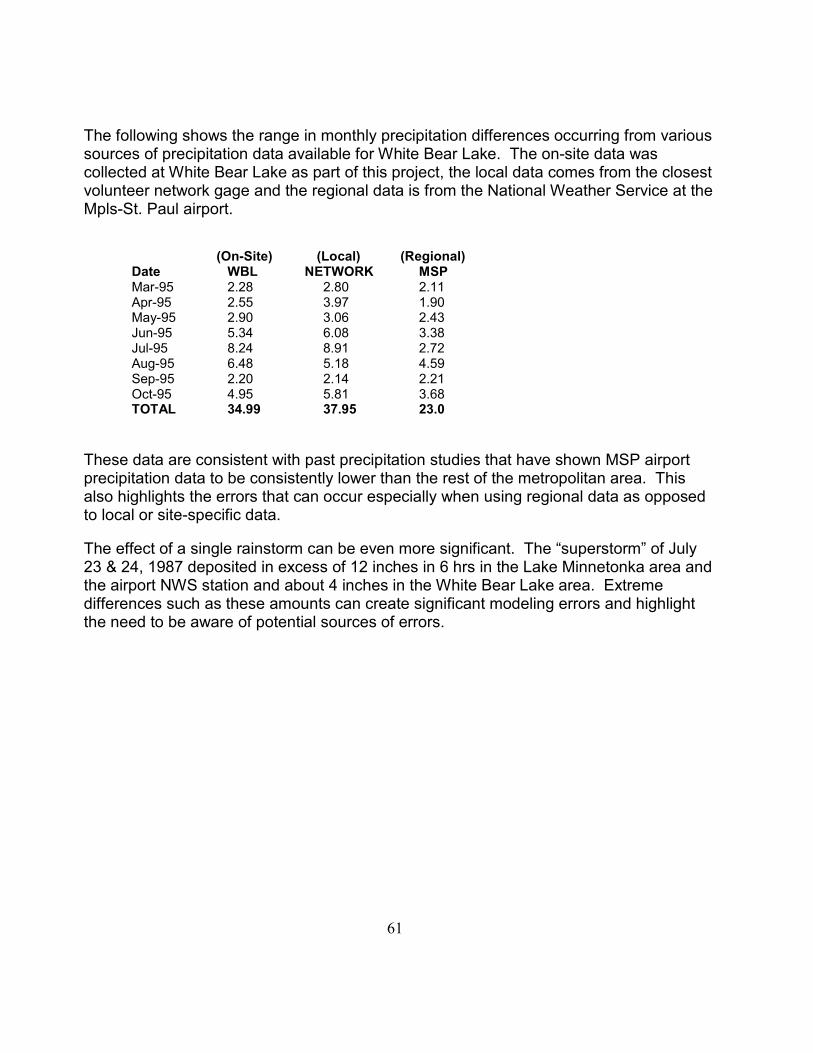
The following shows the range in monthly precipitation differences occurring from various sources of precipitation data available for White Bear Lake. The on-site data was collected at White Bear Lake as part of this project, the local data comes from the closest volunteer network gage and the regional data is from the National Weather Service at the Mpls-St. Paul airport. (On-Site) (Local) (Regional) Date WBL NETWORK MSP Mar-95 2.28 2.80 2.11 Apr-95 2.55 3.97 1.90 May-95 2.90 3.06 2.43 Jun-95 5.34 6.08 3.38 Jul-95 8.24 8.91 2.72 Aug-95 6.48 5.18 4.59 Sep-95 2.20 2.14 2.21 Oct-95 4.95 5.81 3.68 TOTAL 34.99 37.95 23.0 These data are consistent with past precipitation studies that have shown MSP airport precipitation data to be consistently lower than the rest of the metropolitan area. This also highlights the errors that can occur especially when using regional data as opposed to local or site-specific data. The effect of a single rainstorm can be even more significant. The “superstorm” of July 23 & 24, 1987 deposited in excess of 12 inches in 6 hrs in the Lake Minnetonka area and the airport NWS station and about 4 inches in the White Bear Lake area. Extreme differences such as these amounts can create significant modeling errors and highlight the need to be aware of potential sources of errors.

61

Recommendations for future development This project has provided for extensive examination of model capabilities and shortcomings. Especially the shortcomings have been documented throughout the project. Some modifications have been implemented and included in the current version and some would require much more extensive modifications and have been documented for future consideration. The WATBUD program accumulates the various input/outputs of water to a lake volume by using actual observations of such flows or by using sub-models in an attempt to emulate them. The accuracy of such models can be limited by the availability of appropriate observations. For instance, some observations may be very difficult to obtain, or the representativeness of observations may be an unresolvable question, or enhanced observations of certain types may simply be too expensive to support. For many of the flows, several alternative models exist. The alternates may use differing time series of other variables as inputs or may simply have different mathematical forms. -Enhancements to the WATBUD sub-models to improve their accuracy in emulating various physical processes should be a continuing process. For instance, the only evaporation model now available in WATBUD seems to evaporate amounts that are too small in late summer. Some evidence suggests that the real evaporation behavior could perhaps be better emulated by better use of the temperature time series data. -Alternate sub-models should be examined and/or devised which can take advantage of a range of time series data types so that whatever information is available can be fully exploited. -Ground water emulations and ground water exchange sub-models that are not dependant on well-level time series should be devised. -Improvements should be made to the data retrieval systems that are used to form the data sets used as inputs to the WATBUD model. Such retrieval capabilities should be made available 'online', for instance, on the Internet. -The SCS Curve Number method for runoff is known to underestimate runoff for rainstorms less than 12 hours duration. This isn’t as significant for lakes with small watersheds however consideration should be given to other runoff models or to at least modify the procedure for tacking and identifying antecedent runoff conditions. - Modify runoff to be appropriate for larger watersheds by distributing runoff over more than one day.

62

Document Model To make the WATBUD model usable to others in addition to its developers a User’s Manual was developed to provide basic instructions on model capability, setup and use. Detailed help on all model aspects is available through the internal software help files. Availability Effective July 1, 1997 “WATBUD”, introductory documentation and limited technical assistance will be available by contacting DNR Waters at 651-296-4800.

63

Application to PICKEREL LAKE Ottertail County (560204) Concern that pumping from recently installed irrigation wells was causing artificially lower Pickerel Lake levels was investigated by Division of Waters staff. The data collected provided an opportunity to test the usefulness of WATBUD in evaluating the effect of pumping on the water balance of Pickerel Lake. Pumping wells capable of 600 g.p.m. were installed approximately 100 feet north of the lake’s north shore in the surficial aquifer. The aquifer is considered to be fairly well connected to the lake. Data collected during 1995 as part of the Division of Waters well interference investigation were used in WATBUD to estimate effects of pumping on lake levels. The physical lake parameters were determined from the USGS quadrangle map. An estimated hydrologic curve number of 70 and evaporation coefficient of 0.8 were assumed fixed and constant ground water exchange model coefficient was fitted for pumping and non-pumping periods. The calibrated constant ground water exchange was determined to be -0.010 feet/day for the pumping period (Jun 2 to Aug 5) and to be 0.007 feet/day during the non-pumping period (Aug 6 to Sep 25). The net difference of 0.017 feet/day over the 67 day pumping period results in a net lake level reduction of 1.14 feet due to the appropriation pumping. The Observation Well (variable) ground water exchange model was also used to evaluate its capability to simulate ground water exchange transients during pumping and non-pumping periods. It was necessary to use a combination of the Observation Well and constant models to allow the ground water exchange to vary from positive to negative. However, combining the two GWex models worked very well and resulted in very similar ground water exchange volumes during the pumping and non-pumping periods as was simulated by the constant model. In addition, the simulated results of day-to-day transients in ground water - surface water exchange provided through use of the Observation Well model showed this new capability in WATBUD working as anticipated. The following graphs show results of the Pickerel Lake analysis.

64

CONSTANT - entire period (6/2/95 to 9/25/95) GWex= -0.003 ft/day

96

The grathe enteach th P

lake

leve

l

93

94

95

96

e le

vel

lak

93

94

95

J95 A95 S95

PICKERAL LAKE 56-0204 mod: PCKRLWS ts: WL560204

Figure 43

phical output in figure 43 shows the results of using the constant GWex model for ire period while figures 44 and 45 show the results of using the constant model for e pumping and non-pumping periods, respectively.

umping (6/2 to 8/5) Non-pumping (8/6 to 9/25) GWex

96

= -.007 ft/day Figure 44 GWex= 0.010 ft/day Figure 45

J95 A95

PICKERAL LAKE 56-0204 mod: PCKRLS ts: WL560204

65

l

95

lake

leve

93

94

S95

PICKERAL LAKE 56-0204 mod: PCKRLS ts: WL560204

CONSTANT + VARIABLE (6/2 to 9/25)

96

The gravariablesimulatito the u

lake

leve

l

93

94

95

J95 A95 S95

PICKERAL LAKE 56-0204 mod: PCKRLWS ts: WL560204

Figure 46

phical output in figure 46 shows the results of using both the constant and GWex models for the entire period. Note the significant improvement in on, especially during the non-pumping period (Aug 6 - Sept 25), when compared se of the constant model alone on the previous page.

66

The combined GWex (constant and variable) model results can also be generated as tabular data by WATBUD as shown in the following table: (All values are represented as equivalent feet of daily lake level change) PICKEREL LAKE 56-0204 MM/DD/YYYY Precip RO Flow Evap GWex Level Q feet cfs

06/02/95 0 0 0 -0.015 0.009 94.564 0 06/03/95 0 0 0 -0.016 -0.015 94.532 0 06/04/95 0 0 0 -0.018 -0.010 94.504 0 06/05/95 0.004 0 0 -0.017 -0.006 94.485 0 06/06/95 0 0 0 -0.017 -0.003 94.465 0 06/07/95 0.037 0 0 -0.016 0 94.486 0 06/08/95 0 0 0 -0.005 -0.003 94.478 0 06/09/95 0.008 0 0 -0.007 0.005 94.484 0 06/10/95 0.027 0 0 -0.009 0.012 94.513 0 06/11/95 0 0 0 -0.010 0.004 94.507 0 06/12/95 0 0 0 -0.012 0.003 94.499 0 06/13/95 0 0 0 -0.013 0.001 94.487 0 06/14/95 0 0 0 -0.017 -0.006 94.464 0 06/15/95 0 0 0 -0.021 -0.025 94.418 0 06/16/95 0 0 0 -0.019 -0.026 94.372 0 06/17/95 0 0 0 -0.024 -0.028 94.320 0 06/18/95 0 0 0 -0.026 -0.021 94.273 0 06/19/95 0 0 0 -0.024 -0.028 94.221 0 06/20/95 0 0 0 -0.024 -0.033 94.164 0 06/21/95 0 0 0 -0.024 -0.031 94.109 0 06/22/95 0.304 0.022 0 -0.025 0.012 94.552 0 06/23/95 0.002 0 0 -0.020 -0.004 94.530 0 06/24/95 0 0 0 -0.015 -0.013 94.502 0 06/25/95 0.049 0.002 0 -0.016 -0.007 94.544 0 06/26/95 0.008 0 0 -0.016 -0.004 94.532 0 06/27/95 0 0 0 -0.015 -0.006 94.511 0 06/28/95 0.048 0.002 0 -0.014 0.001 94.561 0 06/29/95 0 0 0 -0.013 -0.004 94.545 0 06/30/95 0.012 0 0 -0.011 0 94.545 0

06/ 1995 0.50 0.03 0 -0.48 -0.23 0

07/01/95 0 0 0 -0.014 -0.006 94.525 0 07/02/95 0.083 0 0 -0.010 0.002 94.599 0 07/03/95 0.040 0 0 -0.014 0.008 94.633 0 07/04/95 0.118 0.005 0 -0.016 0.015 94.788 0

MM/DD/YYYY Precip RO Flow Evap GWex Level Q feet cfs

07/08/95 0.005 0 0 -0.016 -0.005 94.814 0 07/09/95 0 0 0 -0.016 -0.004 94.793 0 07/10/95 0 0 0 -0.018 -0.009 94.766 0

67

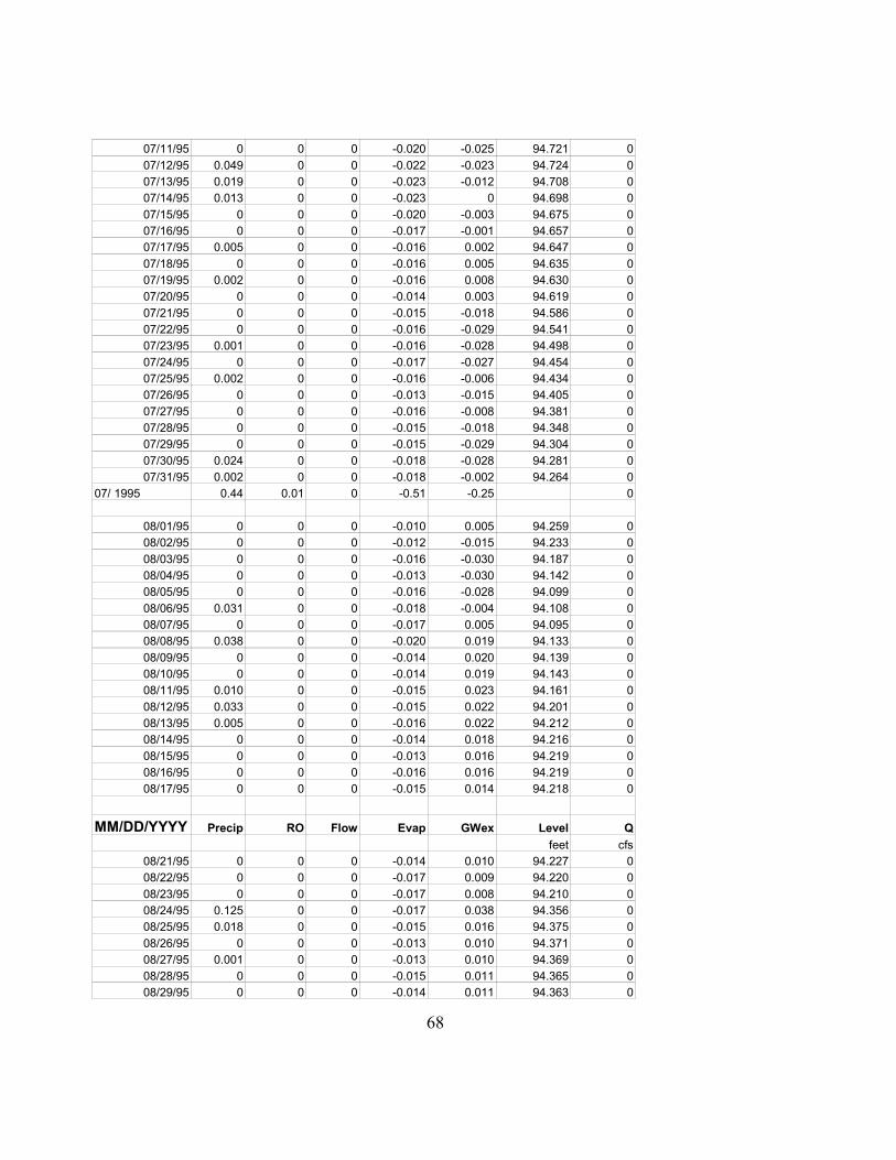
07/11/95 0 0 0 -0.020 -0.025 94.721 0 07/12/95 0.049 0 0 -0.022 -0.023 94.724 0 07/13/95 0.019 0 0 -0.023 -0.012 94.708 0 07/14/95 0.013 0 0 -0.023 0 94.698 0 07/15/95 0 0 0 -0.020 -0.003 94.675 0 07/16/95 0 0 0 -0.017 -0.001 94.657 0 07/17/95 0.005 0 0 -0.016 0.002 94.647 0 07/18/95 0 0 0 -0.016 0.005 94.635 0 07/19/95 0.002 0 0 -0.016 0.008 94.630 0 07/20/95 0 0 0 -0.014 0.003 94.619 0 07/21/95 0 0 0 -0.015 -0.018 94.586 0 07/22/95 0 0 0 -0.016 -0.029 94.541 0 07/23/95 0.001 0 0 -0.016 -0.028 94.498 0 07/24/95 0 0 0 -0.017 -0.027 94.454 0 07/25/95 0.002 0 0 -0.016 -0.006 94.434 0 07/26/95 0 0 0 -0.013 -0.015 94.405 0 07/27/95 0 0 0 -0.016 -0.008 94.381 0 07/28/95 0 0 0 -0.015 -0.018 94.348 0 07/29/95 0 0 0 -0.015 -0.029 94.304 0 07/30/95 0.024 0 0 -0.018 -0.028 94.281 0 07/31/95 0.002 0 0 -0.018 -0.002 94.264 0

07/ 1995 0.44 0.01 0 -0.51 -0.25 0

08/01/95 0 0 0 -0.010 0.005 94.259 0 08/02/95 0 0 0 -0.012 -0.015 94.233 0 08/03/95 0 0 0 -0.016 -0.030 94.187 0 08/04/95 0 0 0 -0.013 -0.030 94.142 0 08/05/95 0 0 0 -0.016 -0.028 94.099 0 08/06/95 0.031 0 0 -0.018 -0.004 94.108 0 08/07/95 0 0 0 -0.017 0.005 94.095 0 08/08/95 0.038 0 0 -0.020 0.019 94.133 0 08/09/95 0 0 0 -0.014 0.020 94.139 0 08/10/95 0 0 0 -0.014 0.019 94.143 0 08/11/95 0.010 0 0 -0.015 0.023 94.161 0 08/12/95 0.033 0 0 -0.015 0.022 94.201 0 08/13/95 0.005 0 0 -0.016 0.022 94.212 0 08/14/95 0 0 0 -0.014 0.018 94.216 0 08/15/95 0 0 0 -0.013 0.016 94.219 0 08/16/95 0 0 0 -0.016 0.016 94.219 0 08/17/95 0 0 0 -0.015 0.014 94.218 0

MM/DD/YYYY Precip RO Flow Evap GWex Level Q feet cfs

08/21/95 0 0 0 -0.014 0.010 94.227 0 08/22/95 0 0 0 -0.017 0.009 94.220 0 08/23/95 0 0 0 -0.017 0.008 94.210 0 08/24/95 0.125 0 0 -0.017 0.038 94.356 0 08/25/95 0.018 0 0 -0.015 0.016 94.375 0 08/26/95 0 0 0 -0.013 0.010 94.371 0 08/27/95 0.001 0 0 -0.013 0.010 94.369 0 08/28/95 0 0 0 -0.015 0.011 94.365 0 08/29/95 0 0 0 -0.014 0.011 94.363 0

68

08/30/95 0 0 0 -0.016 0.010 94.357 0 08/31/95 0 0 0 -0.014 0.011 94.354 0

08/ 1995 0.28 0 0 -0.47 0.28 0

09/01/95 0.001 0 0 -0.014 0.012 94.352 0 09/02/95 0 0 0 -0.014 0.007 94.345 0 09/03/95 0 0 0 -0.016 0.008 94.338 0 09/04/95 0 0 0 -0.017 0.008 94.329 0 09/05/95 0.022 0 0 -0.017 0.012 94.346 0 09/06/95 0.010 0 0 -0.015 0.014 94.356 0 09/07/95 0 0 0 -0.009 0.014 94.361 0 09/08/95 0 0 0 -0.007 0.012 94.367 0 09/09/95 0 0 0 -0.006 0.008 94.368 0 09/10/95 0 0 0 -0.007 0.006 94.367 0 09/11/95 0 0 0 -0.009 0.005 94.363 0 09/12/95 0 0 0 -0.012 0.002 94.353 0 09/13/95 0 0 0 -0.013 0.004 94.344 0 09/14/95 0 0 0 -0.009 0.005 94.341 0 09/15/95 0.047 0 0 -0.009 0.015 94.394 0 09/16/95 0 0 0 -0.012 0.007 94.390 0 09/17/95 0 0 0 -0.005 0.009 94.394 0 09/18/95 0 0 0 -0.006 0.005 94.393 0 09/19/95 0 0 0 -0.007 0.005 94.391 0 09/20/95 0 0 0 -0.004 0.007 94.394 0 09/21/95 0.006 0 0 -0.004 0.010 94.407 0 09/22/95 0 0 0 -0.002 0.003 94.407 0 09/23/95 0 0 0 -0.005 0.003 94.405 0 09/24/95 0 0 0 -0.004 0.002 94.403 0 09/25/95 0 0 0 -0.005 0.001 94.399 0

69

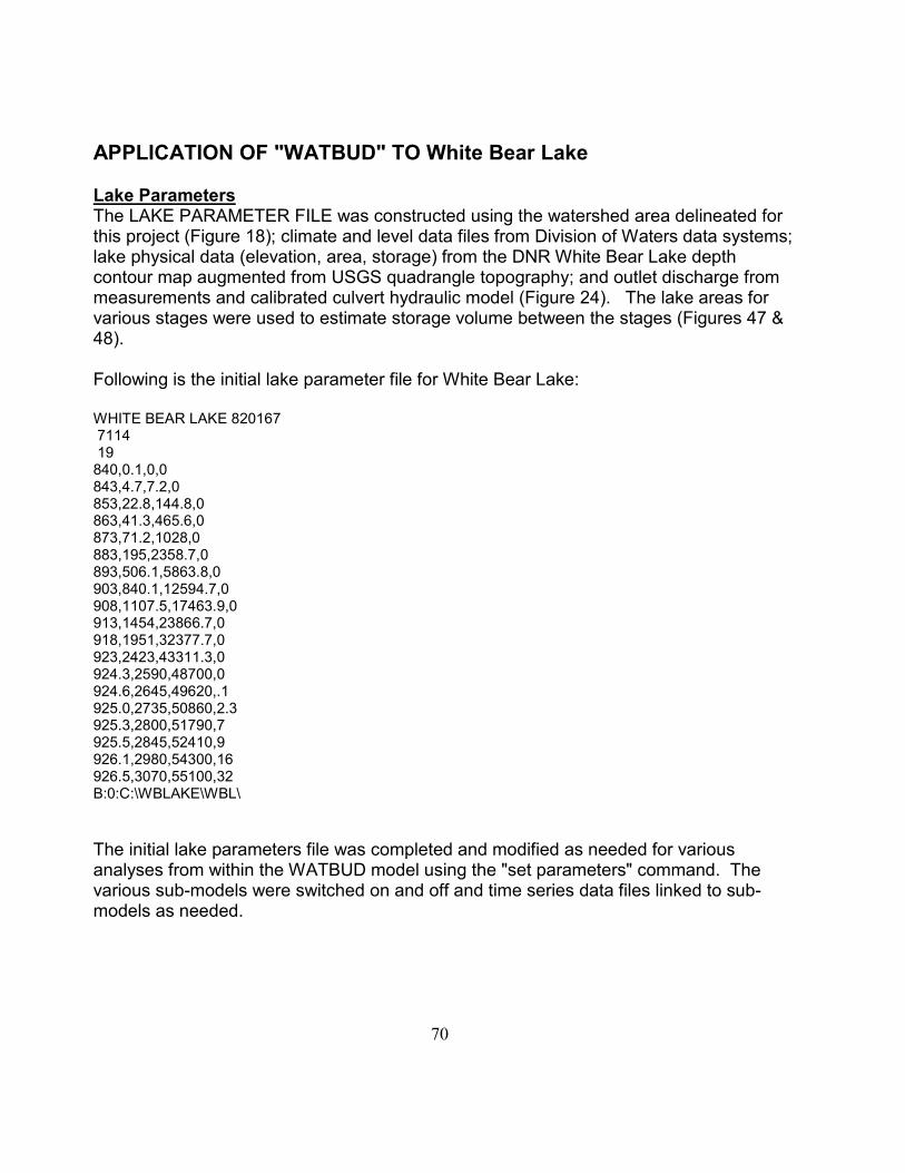
APPLICATION OF "WATBUD" TO White Bear Lake Lake Parameters The LAKE PARAMETER FILE was constructed using the watershed area delineated for this project (Figure 18); climate and level data files from Division of Waters data systems; lake physical data (elevation, area, storage) from the DNR White Bear Lake depth contour map augmented from USGS quadrangle topography; and outlet discharge from measurements and calibrated culvert hydraulic model (Figure 24). The lake areas for various stages were used to estimate storage volume between the stages (Figures 47 & 48). Following is the initial lake parameter file for White Bear Lake: WHITE BEAR LAKE 820167 7114 19 840,0.1,0,0 843,4.7,7.2,0 853,22.8,144.8,0 863,41.3,465.6,0 873,71.2,1028,0 883,195,2358.7,0 893,506.1,5863.8,0 903,840.1,12594.7,0 908,1107.5,17463.9,0 913,1454,23866.7,0 918,1951,32377.7,0 923,2423,43311.3,0 924.3,2590,48700,0 924.6,2645,49620,.1 925.0,2735,50860,2.3 925.3,2800,51790,7 925.5,2845,52410,9 926.1,2980,54300,16 926.5,3070,55100,32 B:0:C:\WBLAKE\WBL\ The initial lake parameters file was completed and modified as needed for various analyses from within the WATBUD model using the "set parameters" command. The various sub-models were switched on and off and time series data files linked to sub-models as needed.

70

71

The following WATBUD output describes sub-models, data and files used in the White

Bear Lake WATBUD analysis for the 1980 decade: WHITE BEAR LAKE 820167 Using lake parameters file C:\White Bear Lake\White Bear LakeCAL80.WTB Watershed area = 7114 acres Lake Levels Time series file: L820167E Field: ELEVATION Precipitation 1 * File: White Bear Lake Field: PRECIP accum T thresh: 30 melt T thresh: 36 melt T multip: .017 Tmin: file: White Bear Lake field: TMIN Tmax: file: White Bear Lake field: TMAX Lake Evaporation Blaney-Criddle Tmin: file: White Bear Lake field: TMIN Tmax: file: White Bear Lake field: TMAX Runoff watershed area relative weight: 1 SCS Curve numbers (D,N,W) = 65.8 82 92.2 combined precip model: 1 * File: White Bear Lake Field: PRECIP Snow Melt Abstraction abstraction: .7 CN - snowmelt: 100 Ground water exchange area (acres): 2400 (approx. feet of lake level change) feet cfs

72

Calibration Best-fit calibrations were completed for each year of decades 1981 to 1990 and 1931 to 1940 (augmentation years). Submodel coefficients were initially set based on regional experience and literature values. A May through September calibration period was used with WATBUD’s optimization routine to calibrate “summer” sub-model coefficients (SCS runoff curve number[CN], and constant ground water exchange[GWex]) and a December through March period was used to calibrate the “winter” models (snow accumulation temperature[Ta], snow melt temperature[Tm], snow melt rate[Mr], snow abstraction[Sa], snowmelt curve number[SCN] and constant ground water exchange[GWex]). Blaney - Criddle evaporation[BC] was fixed at 0.65 based on the results of the project evaporation study. The two calibrations of GWex for each year provided independent GWex values and additional insight to model variability and sensitivity. Submodel coefficients were also manually varied to provide additional insight as to sensitivity. For each decade, average values of the initial calibrated summer and winter sub-model parameters were averaged then fixed and GWex for each year computed. Results from the annual GWex final calibrations for the decade of the 1980's are as follows: 82 SCS runoff curve number[CN] 0.65 Blaney - Criddle evaporation[BC] -.0025 Constant ground water exchange[GWex] - feet/day 30 Snow accumulation temperature[Ta] 36 Snow melt temperature[Tm] 0.017 Snow melt rate[Mr] 0.7 Snow abstraction[Sabs] 100 Snowmelt curve number[SCN]

73

White Bear Lake Ground Water Exchange Constant ground water exchange is estimated with fewer errors using only winter months than when including non-winter months. Because sub-freezing temperatures, for the most part, prohibit precipitation and runoff from entering the lake and ice cover eliminates water loss due to evaporation (small amounts do however occur due to sublimation), the ground water component of a lake's water budget is the principle factor affecting level changes. Lake level augmentation by pumping into the lake from ground water sources occurred during many winters. Because these operations artificially affected level changes, it is expected these would also affect the ground water exchange of the lake during these years resulting in different rates from years or periods without augmentation. It is thought by some the augmentation increases the exchange rate by increasing lake levels and decreasing ground water levels and the increased head differential results in a greater lake volume loss to groundwater. The following table compares winter ground water exchange (lake volume loss) results for the two periods based on the calibrated or fixed parameters for each decade. With Augmentation: Without Augmentation: “1930's” (Jan 1- Mar 15) “1980's” (Jan 1- Mar 15) BC=0.65, CN=79, Ta=29, Tm=33 BC=0.65, CN=82, Ta=30, Tm=36 Mr=0.018, Sabs=.8, SCN=100 Mr=0.017, Sabs=.7, SCN=100 Year GWex Year GWex feet/day in/yr feet/day in/yr 1931 -0.0065 -28.5 1981 -0.0025 -11.0 1932 -0.0078 -34.2 1982 0.001 4.4 1933 -0.0112 -49.1 1983 0.001 4.4 1934 -0.0121 -53.0 1984 0 0.0 1935 -0.0123 -53.9 1985 -0.0007 -3.1 1936 -0.0062 -27.2 1986 -0.0017 -7.4 1937 -0.0042 -18.4 1987 -0.0024 -10.5 1938 -0.0047 -20.6 1988 -0.0024 -10.5 1939 -0.0064 -28.0 1989 -0.0011 -4.8 1940 -0.0049 -21.5 1990 -0.0026 -11.4 Avg -0.0076 -33.4 Avg -0.0011 -5.0 The identified difference in average GWex between the decade of the 80's when no augmentation occurred (-5.0 inches\year) and the 30's when continuous augmentation occurred (-33.4 inches/year) may be quantification of the impact of augmentation from groundwater. From 1931 through 1940 the average annual augmentation was 32.7 inches per year over the surface of the lake. If the difference in volume loss is exclusively due to the augmentation, then the

74

augmentation efficiency would be (32.7-28.0)/32.7= .14 or 14 percent. Very similar results are obtained when identical sub-model coefficients are used as opposed to the above, which were calibrated for each period. Groundwater levels could simply have been naturally lower during the 30's than the 80's and result in this differential. This hypothesis however is inconsistent with the lower lake levels that occurred during the 80's dry period and the likelihood of lowered ground water levels in the 80's due to increased ground water appropriation for domestic and industrial water use.

75

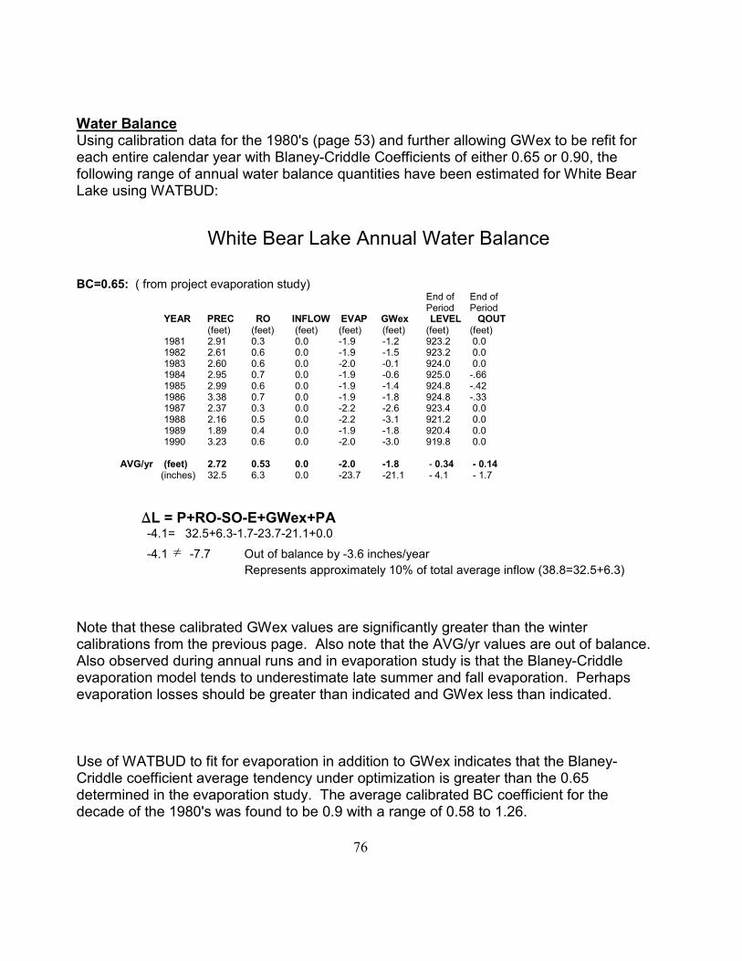
Water Balance Using calibration data for the 1980's (page 53) and further allowing GWex to be refit for each entire calendar year with Blaney-Criddle Coefficients of either 0.65 or 0.90, the following range of annual water balance quantities have been estimated for White Bear Lake using WATBUD:

White Bear Lake Annual Water Balance BC=0.65: ( from project evaporation study) End of End of Period Period YEAR PREC RO INFLOW EVAP GWex LEVEL QOUT (feet) (feet) (feet) (feet) (feet) (feet) (feet) 1981 2.91 0.3 0.0 -1.9 -1.2 923.2 0.0 1982 2.61 0.6 0.0 -1.9 -1.5 923.2 0.0 1983 2.60 0.6 0.0 -2.0 -0.1 924.0 0.0 1984 2.95 0.7 0.0 -1.9 -0.6 925.0 -.66 1985 2.99 0.6 0.0 -1.9 -1.4 924.8 -.42 1986 3.38 0.7 0.0 -1.9 -1.8 924.8 -.33 1987 2.37 0.3 0.0 -2.2 -2.6 923.4 0.0 1988 2.16 0.5 0.0 -2.2 -3.1 921.2 0.0 1989 1.89 0.4 0.0 -1.9 -1.8 920.4 0.0 1990 3.23 0.6 0.0 -2.0 -3.0 919.8 0.0 AVG/yr (feet) 2.72 0.53 0.0 -2.0 -1.8 - 0.34 - 0.14 (inches) 32.5 6.3 0.0 -23.7 -21.1 - 4.1 - 1.7 �L = P+RO-SO-E+GWex+PA -4.1= 32.5+6.3-1.7-23.7-21.1+0.0 -4.1 � -7.7 Out of balance by -3.6 inches/year Represents approximately 10% of total average inflow (38.8=32.5+6.3) Note that these calibrated GWex values are significantly greater than the winter calibrations from the previous page. Also note that the AVG/yr values are out of balance. Also observed during annual runs and in evaporation study is that the Blaney-Criddle evaporation model tends to underestimate late summer and fall evaporation. Perhaps evaporation losses should be greater than indicated and GWex less than indicated. Use of WATBUD to fit for evaporation in addition to GWex indicates that the Blaney-Criddle coefficient average tendency under optimization is greater than the 0.65 determined in the evaporation study. The average calibrated BC coefficient for the decade of the 1980's was found to be 0.9 with a range of 0.58 to 1.26.

76

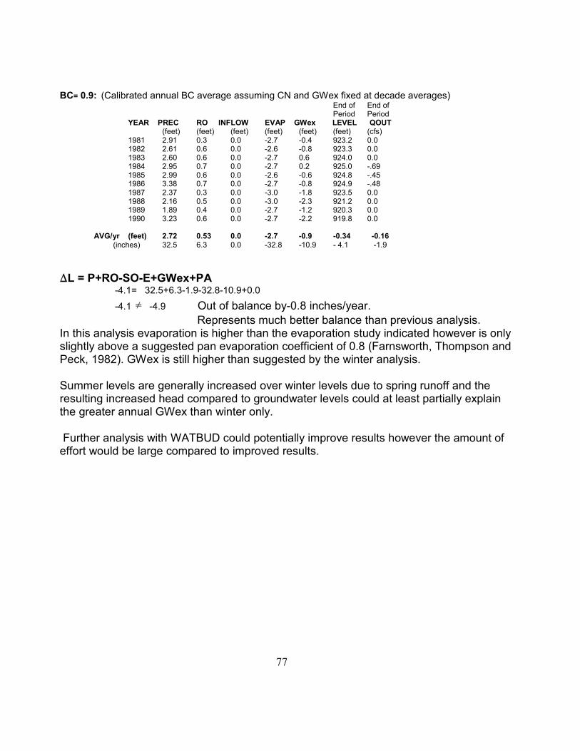
BC= 0.9: (Calibrated annual BC average assuming CN and GWex fixed at decade averages) End of End of Period Period YEAR PREC RO INFLOW EVAP GWex LEVEL QOUT (feet) (feet) (feet) (feet) (feet) (feet) (cfs) 1981 2.91 0.3 0.0 -2.7 -0.4 923.2 0.0 1982 2.61 0.6 0.0 -2.6 -0.8 923.3 0.0 1983 2.60 0.6 0.0 -2.7 0.6 924.0 0.0 1984 2.95 0.7 0.0 -2.7 0.2 925.0 -.69 1985 2.99 0.6 0.0 -2.6 -0.6 924.8 -.45 1986 3.38 0.7 0.0 -2.7 -0.8 924.9 -.48 1987 2.37 0.3 0.0 -3.0 -1.8 923.5 0.0 1988 2.16 0.5 0.0 -3.0 -2.3 921.2 0.0 1989 1.89 0.4 0.0 -2.7 -1.2 920.3 0.0 1990 3.23 0.6 0.0 -2.7 -2.2 919.8 0.0 AVG/yr (feet) 2.72 0.53 0.0 -2.7 -0.9 -0.34 -0.16 (inches) 32.5 6.3 0.0 -32.8 -10.9 - 4.1 -1.9 �L = P+RO-SO-E+GWex+PA -4.1= 32.5+6.3-1.9-32.8-10.9+0.0 -4.1 � -4.9 Out of balance by-0.8 inches/year. Represents much better balance than previous analysis. In this analysis evaporation is higher than the evaporation study indicated however is only slightly above a suggested pan evaporation coefficient of 0.8 (Farnsworth, Thompson and Peck, 1982). GWex is still higher than suggested by the winter analysis. Summer levels are generally increased over winter levels due to spring runoff and the resulting increased head compared to groundwater levels could at least partially explain the greater annual GWex than winter only. Further analysis with WATBUD could potentially improve results however the amount of effort would be large compared to improved results.

77

Future Levels WATBUD has the capability of estimating the exceedance probability of future lake levels. On landlocked lakes or those nearly landlocked as White Bear Lake is, the lake level during any year is dependent on the lake level at the beginning of that year in addition to hydrologic conditions throughout the year. Once a lakes’ sub-model coefficients are determined, the specified model is initialized with a starting lake level, that will be used as beginning level of each segment, and WATBUD will 'run forward' with segments of historic climate data to construct a family of potential end of run period lake levels. The segment length is established by start and end dates. The family of potential levels is used with statistical methods to quantify the ranking of level exceedance of the end-of-period potential levels and is displayed and saved as graphical output. Tabular output include the estimated end of period, maximum and minimum levels occurring during each segment which the user can use with external analysis methods. The maximum and minimum levels are especially useful for estimating the probability of flood or drought levels. Using White Bear Lake average sub-model coefficients from the 1980's calibration and the run-out elevation (924.3 feet) as the period initial lake level, the probability of lake levels over the ensuing year was estimated for average, maximum and minimum annual GWex values. The following graphical model output shows the probability of end-of-segment levels for the average GWex assumption. AVERAGE

927GWex Figure 49

lake

leve

l

923

924

925

926

2 11 20 29 38 47 56 65 74 83 92 101

WHITE BEAR LAKE 820167 EXCEEDANCES

78

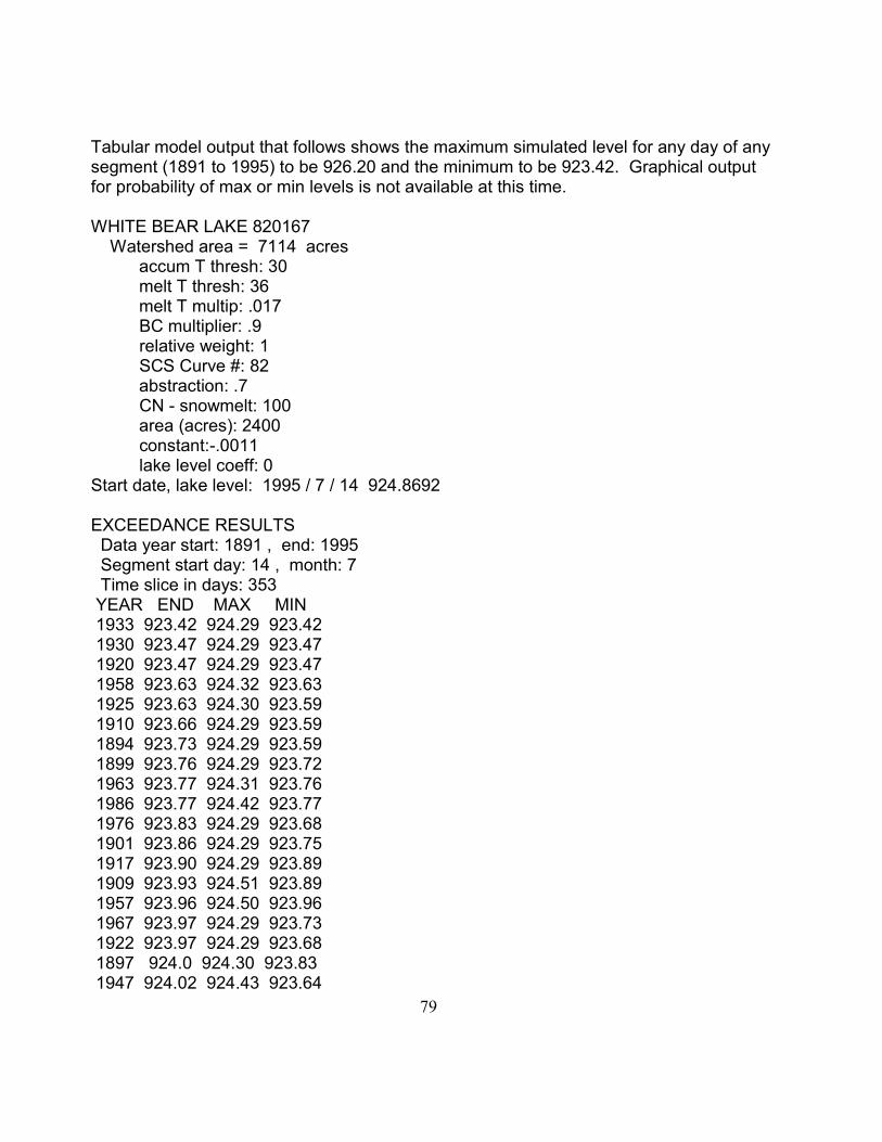
Tabular model output that follows shows the maximum simulated level for any day of any segment (1891 to 1995) to be 926.20 and the minimum to be 923.42. Graphical output for probability of max or min levels is not available at this time. WHITE BEAR LAKE 820167 Watershed area = 7114 acres accum T thresh: 30 melt T thresh: 36 melt T multip: .017 BC multiplier: .9 relative weight: 1 SCS Curve #: 82 abstraction: .7 CN - snowmelt: 100 area (acres): 2400 constant:-.0011 lake level coeff: 0 Start date, lake level: 1995 / 7 / 14 924.8692 EXCEEDANCE RESULTS Data year start: 1891 , end: 1995 Segment start day: 14 , month: 7 Time slice in days: 353 YEAR END MAX MIN 1933 923.42 924.29 923.42 1930 923.47 924.29 923.47 1920 923.47 924.29 923.47 1958 923.63 924.32 923.63 1925 923.63 924.30 923.59 1910 923.66 924.29 923.59 1894 923.73 924.29 923.59 1899 923.76 924.29 923.72 1963 923.77 924.31 923.76 1986 923.77 924.42 923.77 1976 923.83 924.29 923.68 1901 923.86 924.29 923.75 1917 923.90 924.29 923.89 1909 923.93 924.51 923.89 1957 923.96 924.50 923.96 1967 923.97 924.29 923.73 1922 923.97 924.29 923.68 1897 924.0 924.30 923.83 1947 924.02 924.43 923.64

79

1912 924.04 924.35 923.87 1975 924.04 924.54 923.81 1913 924.05 924.37 923.86 1929 924.07 924.31 923.84 1938 924.07 924.29 923.76 1937 924.09 924.39 923.72 1923 924.10 924.33 923.62 1924 924.13 924.45 924.04 1931 924.13 924.63 923.75 1969 924.15 924.51 923.55 1936 924.15 924.39 923.60 1906 924.15 924.29 923.86 1954 924.16 924.53 923.98 1939 924.18 924.30 923.77 1962 924.19 924.49 924.15 1932 924.19 924.68 923.69 1914 924.20 924.38 923.85 1943 924.23 924.49 923.91 1921 924.25 924.63 923.98 1980 924.28 924.59 924.08 1987 924.31 925.12 924.20 1940 924.36 924.78 923.74 1959 924.37 924.47 924.03 1928 924.40 924.64 924.01 1960 924.41 924.67 923.90 1935 924.43 924.85 923.75 1948 924.43 924.88 923.93 1979 924.48 924.78 924.02 1988 924.49 924.84 924.05 1956 924.50 924.64 924.10 1893 924.51 925.09 923.75 1916 924.52 924.69 923.66 1971 924.55 924.99 923.90 1891 924.56 924.64 923.81 1908 924.59 924.79 923.84 1965 924.61 925.06 924.05 1981 924.62 925.17 924.18 1946 924.62 924.88 923.90 1968 924.63 925.20 923.93 1927 924.63 925.13 923.91 1900 924.64 924.77 923.96 1945 924.67 924.78 923.95 1955 924.71 924.74 923.91

80

1911 924.74 925.32 924.24 1952 924.76 925.03 923.69 1926 924.77 924.97 924.14 1993 924.77 925.38 924.10 1972 924.77 925.12 924.26 1904 924.78 924.95 924.15 1895 924.81 925.24 923.97 1902 924.81 925.20 924.10 1918 924.82 925.40 924.08 1973 924.83 925.10 923.92 1953 924.84 924.94 923.62 1983 924.84 925.09 923.85 1978 924.86 924.94 923.82 1989 924.86 925.03 923.79 1970 924.87 925.06 923.83 1961 924.90 925.12 923.92 1995 924.92 925.26 924.29 1990 924.94 925.20 924.11 1892 924.95 925.79 924.21 1949 924.95 925.59 923.97 1934 924.95 925.25 923.79 1966 924.96 925.04 923.87 1898 924.97 925.22 923.80 1994 924.97 925.17 924.02 1942 924.97 925.31 924.16 1984 924.98 925.23 923.85 1907 925.0 925.07 924.17 1991 925.02 925.70 924.09 1903 925.03 925.34 924.16 1982 925.03 925.52 923.94 1941 925.07 925.33 923.93 1944 925.08 925.10 923.80 1915 925.11 925.33 924.06 1950 925.14 925.20 923.87 1951 925.14 925.72 924.16 1919 925.27 925.27 923.93 1992 925.29 925.31 924.13 1905 925.31 925.64 924.08 1985 925.37 925.78 924.08 1964 925.43 926.29 923.92 1896 925.43 925.68 924.0 1974 925.80 925.88 923.83 1977 926.09 926.20 924.07

81

CONCLUSIONS Augmentation increases White Bear Lake levels. Visual comparisons of lake level data during winters of no augmentation (1980's) to levels during winters with augmentation (1930's) shows significant level increases during augmentation periods and little increase during periods of no augmentation. It is also clear however that augmentation is not 100% effective and increased levels due to augmentation are only temporary.

Winter ground water exchange analyses for each year during the 1930's and 1980's were completed. The 1930's represented a period of nearly continuous augmentation and the 1980's had no augmentation. These WATBUD analyses show ground water exchange (GWex) at White Bear Lake varies from year to year.

The average estimated loss to ground water is 5 inches per year over the ten year period of 1981 to 1990, the maximum loss was 11.4 inches per year (1990) and the minimum was actually a gain of 4.4 inches per year (1982 and 1983).

During the 1930's, White Bear Lake lost an average of 33 inches per year to ground water. The maximum estimated loss is 54 inches per year in 1935 and the minimum was 18 inches per year in 1937.

Augmentation at White Bear Lake appears to increase water loss from the lake to ground water. If this increased loss from the lake is totally due to augmentation effects (increased head differential resulting from higher lake levels and lower ground water level due to augmentation pumping), then 86% of the augmentation water is lost due to the pumping-induced increased loss rate to groundwater. Put another way, the effectiveness of augmentation in terms of volume added to the lake in any year is estimated by WATBUD analysis to be 14%.

The efficiency of augmentation volume to lake level change is difficult to assess in greater detail due to lack of data (especially ground water levels) during augmentation. In fact, this efficiency likely varies with time as do several other factors of the water balance.

It is also apparent that any level increase due to augmentation is not everlasting and likely is dissipated relatively quickly. The effect of augmentation has been described as having a half-life of one year (Hill, 1993).

The ground water exchange difference (from the 1930's to the 1980's) may also be due to substantially lower ground water levels during the 1930's than existed during the 1980's. Data is not available to support or refute this potential condition. The sustained dry conditions of the 30's persisted longer than any more recent dry period and it is possible

82

ground water levels in the 1930's were lower than in the 1980's due to these conditions.

MODFLOW modeling results indicate increased use of ground water via high capacity wells for municipal water supply and commercial use has resulted in lower ground water levels.

Over the long term (years, decades), White Bear Lake levels are controlled principally by the region's ground water level fluctuations and in the short term (monthly, seasonally) by the surficial elements of the lake water balance parameters (which include precipitation, runoff and augmentation).

Because White Bear Lake levels above elevation 925 have been documented prior to the mid-1920's when Ramsey County began level augmentation via ground water, it is reasonable to assume that ground water exchange and level conditions existed at that time adequate to produce those lake levels. The key to ensuring that White Bear Lake levels can continue to at least periodically exceed elevation 924 or 925 is contingent on ensuring ground water levels do not permanently drop to levels similar to those resulting from the drought of the late 1980's.

The two-foot reduction in the outlet control elevation since 1940 has significantly reduced the height and duration of extreme high levels and likely has no significant effect on extreme low levels.

The increase in drainage area compared to that documented in 1924 will tend to generally increase levels and level duration. It will likely not affect low levels because during dry climate conditions the additional areas now draining to the lake will likely have receded to a level where they will no longer contribute drainage to the lake.

The future levels capability of WATBUD provides a unique modeling capability for estimating probabilities of flood levels on landlocked or nearly landlocked lakes.

The implemented variable ground water exchange sub-model has been shown, through the Pickerel Lake application, to simulate the surface water/ground water exchange dynamics resulting from short term ground water pumping near the lake.

During a peer review meeting, it was noted White Bear Lake might not be a good initial example to apply WATBUD due to the lake’s complex geology. Attempts at application at White Bear Lake seem to be at least partially substantiating this noted complexity. The variable ground water sub-model shows significant improvement in simulating long-term level changes at White Bear Lake than afforded by the constant ground water sub-model.

A major concern of local residents, and at least a partial reason for initiation of this

83

project, was that White Bear Lake levels would not return to normal levels following the 1988, 1989 drought. The White Bear Lake area climate caused levels to exceed elevation 923 by 1993 and levels high enough to outflow by Fall, 1995 and continued outflow into 1996. How long levels above elevation 925 or 924 or 923 will be sustained is subject to the vagaries of long-term precipitation and other factors affecting local ground water levels. These factors certainly include long-term impacts of future ground water appropriations.

Ground water or Surface water models typically in use today, with few exceptions, do not provide simulation of the dynamic characteristics of the other component. The need for models capable of simulating the dynamics of both surface water and ground water is identified in reviewed literature. In a few cases, models have been developed, however they are generally not available for use by others. WATBUD is a tool developed to assist in filling the existing void in models that do not account for surface water/ground water dynamics.

Ultimately we need to begin to consider the concept of not only the water balance of lakes or surface water systems but also that of ground water systems. To accomplish this, improved knowledge of ground water recharge and discharge in addition to the ability to model multiple layers of groundwater systems is needed. For surface and ground water systems, improved understanding is contingent on available data documenting the resource characteristics and analytical expertise. The data collected and presented in this report and analyses completed are just one step of many in this process.

84

BIBLIOGRAPHY Allred, E.R. and Manson, P.W. and Schwartz, G.M. and Golany, P. and Reinke, J.W. 1971, “Hydrology of Ponds and Small Lakes”. Baker, D.G. and Nelson, W.W. and Kuehnast, E.L. 1979. Climate of Minnesota. Brown, R.G., 1985, Hydrologic Factors Affecting Lake-Level Fluctuations in Big Marine Lake, Washington County, Minnesota. Coates, P.N., 1924. Special Report on Lake Improvement. Eckman, Julie, 1996, “The White Bear Lake Project: A Systems Approach...” . Eckman, Julie, 1996, “Hueristics used in Developing Computer Simulations for Predicting Lake Levels”. Farnsworth, R.K. and Thompson, E.S. and Peck, E.L. 1982. Evaporation Atlas for the Contiguous 48 United States. Food and Agriculture Organization for the United Nation (FAO, Clarke, R.T), 1973 Mathematical Models in Hydrology, pp 156-159. Hill, J.Stanley, “A Mathematical Model of White Bear Lake Levels”, 1991. Hill, J.Stanley, “A Study of White Bear Lake Levels”, 1993. Koestner, F. 1995. “The White Bear Lake Study”. McWhorter, D.B. and Sunada, D.K. 1977. Ground-Water Hydrology and Hydraulics. Hounam, C.E., 1973, Comparison Between Pan and Lake Evaporation. Manson, P.W. and Schwartz, G.M. and Allred, E.R. 1968, “Hydrology of Ponds and Small Lakes”. Minnesota DNR, Division of Waters, “The Effects of Lake Level Lowering on Lake- Ground Water Interaction at School Section Lake, Stearns County, Minnesota”, January 1986.

85

Setterholm, Dale, Report to White Bear Lake Conservation District: “Lake Level Controls and Pumping”, 1993. Winter, T. C. 1981. “Uncertainties in Estimating the Water Balance of Lakes”, P.s. 82-115. United States Department of Agriculture, National Engineering Handbook, Section 4 - Hydrology, March 1985. United States Department of Agriculture, 1986. “Urban Hydrology for Small Watersheds, Chapter 2: Estimating Runoff”.

86

Selected Bibliography on Ground water seepage and Modeling Almendinger, J. E. 1990. Ground water control of Closed-Basin Lake Levels Under Steady-State Conditions. Journal of Hydrology, 112: 293-318. This paper uses a steady-state, 2-D, analytic element model to look at how sensitive lake levels are to local and regional factors. Lake size, distance from a river, net surface recharge, and regional ground water recharge are considered and evaluated. Anderson, M. P., and Cheng, X. 1993. Long- and short-term transience in a ground water/lake system in Wisconsin, USA. Journal of Hydrology, 145: 1-18. This article discusses a 10 year lake study which looked at the development of ground water mounds adjacent to the shores of Crystal Lake and its affect on ground water seepage. Transient effects of greater precipitation in wet years created GW mounds which induced greater net seepage into the lake. Drier years showed a lack of GW mounding and less seepage to the lake. Anderson, M. P. and Munter, J. A. 1981. Seasonal Reversals of Ground water Flow Around Lakes and the Relevance to Stagnation Points and Lake Budgets. Water Resources Research. 17(4) : 1139-1150. Anderson, M. P. and Woessner, W. W. 1992. Applied Ground water modeling. Academic Press, Inc. 381 p. Barwell, V. K. and Lee, R.D. 1981. Determination of Horizontal-to-Vertical Hydraulic Conductivity Ratios from Seepage Measurements on Lake Beds. Water Resources Research 17(3): 565-570. Belanger, T. V. and Montgomery, M. T. 1992. Seepage meter errors. Limnology and Oceanography 27(8): 1787-1795. Belanger, T. V. and R. A. Kirkner. 1994. Ground water/Surface Water interaction in a Florida Augmentation Lake. Lake and Reservoir Management. 8(2) : 165-174. Born, S. M., Smith, S. A., and Stephenson, D. A. 1979. Hydrogeology of Glacial-Terrain Lakes, with Management and Planning Applications. Journal of Hydrology, 43: 7-43. Brown, R.G. 1985. Hydrologic Factors Affecting Lake-Level Fluctuctuations in Big Marine Lake, Washington County, Minnesota. U.S. Geological Survey. Water-Resources Investigations Report 85-4176. This report describes the physical setting and hydrogeology of Big Marine Lake. Geochemistry data of the Prairie du Chien-Jordan aquifer, drift aquifer and the lake are compared to provide insight into ground water movement. Historical trends of precipitation and stream levels are compared to historic lake levels to provide evidence of the connection of ground water to the lake. Cheng, X. and Anderson, M. P. 1993. Numerical Simulation of Ground-Water Interaction

87

with Lakes Allowing for Fluctuating Lake Levels. Ground water 31(6): 929-933. The authors describe a new module for MODFLOW that allows the simulation of steady-state and transient ground waterflow with fluctuating lake levels. Cherkauer, D. S. and Nader, D. C. 1989. Distribution of Ground water Seepage to Large Surface-Water Bodies: The Effect of Hydraulic Heterogeneities. Journal of Hydrology, 109: 151-165. Cherkauer, D. S. and Zanger, A. P. 1989. Ground waterInteraction with a Kettle-Hole Lake: Relation of Observations to Digital Simulations. Journal of Hydrology, 109: 167-184. Downing, J. A., and Peterka, J. J. 1978. Relationship of rainfall and lake ground waterseepage. Limnology and Oceanography 23(4): 821-825. Fokkens, B. and Weijenberg, J. 1968. Measuring the Hydraulic Potential of Ground water with the Hydraulic Potential Probe. Journal of Hydrology, 6: 306-313. Guswa, J. H., Siegel, D. I., and Gillies, D. C. 1982. Preliminary Evaluation of the Ground-Water-Flow System in the Twin Cities Metropolitan Area, Minnesota. U.S. Geological Survey Water Resources Investigations Report 82-44. This report examines the hydrogeology and physical setting of the main Twin Cities aquifers and uses this information to build a steady state finite difference ground water flow model (pre-MODFLOW). The model output is compared to observed potentiometric levels to devise residuals of error for each modeled cell. 1885 pre-ground water development and a 1971-1977 extensive ground water development simulations are run. The last part summarizes water chemistry of the major Twin Cities aquifers and provides concentration contour maps. Fukuo, Y. and Kaihotsu, I. 1988. A theoretical Analysis of Seepage Flow of the Confined Ground water into the Lake Bottom With a Gentle Slope. Water Resources Research, 24(11): 1949-1953. Jaquet, N. G. 1976. Ground-Water and Surface-Water Relationships in the Glacial Province of Northern Wisconsin - Snake Lake. Ground water, 14(4): 194-199. Kanavetsky, R., Walton, M. 1978. Hydrogeologic map of Minnesota - Bedrock hydrogeology, Minnesota Geological Survey, University of Minnesota. Kenoyer, G. J. and Anderson, M. P. 1989. Ground water’s Dynamic Role in Regulating Acidity and Chemistry in a Precipitation-Dominated Lake. Journal of Hydrology, 109: 287-306. Krabbenhoft, D. P., Bowser, C. J., Anderson, M.P., and Valley, J. W. 1990. Estimating Ground water exchange With Lakes 1. The Stable Isotope Mass Balance Method. Water Resources Research, 26(10): 2445-2453. Krabbenhoft, D. P., Bowser, C. J., Anderson, M.P., and Valley, J. W. 1990. Estimating Ground water exchange With Lakes 2. Calibration of a Three-Dimensional, solute

88

Transport Model to a Stable Isotope Plum. Water Resources Research, 26(10): 2455-2462. Krabbenhoft, D. P. and Anderson, M.P. 1986. Use of a Numerical Ground-Water Flow Model for Hypothesis Testing. Ground water, 24(1): 49-55. Larson, S. P., McBride, M. S., and Wolf, R. J. 1975. Digital Models of a Glacial Outwash Aquifer in the Pearl-Sallie Lakes Area, West-Central Minnesota. U.S. Geological Survey Water Resources Investigations Report 40-75. This report applies a steady-state two-dimensional ground water flow model to lakes in the Alexandria moraine complex. The 2-D areal model uses constant head nodes to model lake cells that are in good connection to the aquifer. Cells that are not in good connection used the lake level as a hydraulic head above a confined aquifer. A vertical flow model was set up using Richards’ equation. Data from seepage meters (taken by Lee, D. R.) are compared to modeled seepage rates from shore towards the interior of Lake Sallie. Lee, D. R. 1977. A Device for Measuring Seepage Flux in Lakes and Estuaries. Limnology and Oceanography 23(4): 821-825. Lee, D. R. and Cherry, J. A. 1978. A Field Exercise on Ground water flow Using Seepage Meters and Mini-piezometers. Journal of Geological Education, 27: 6-10. Lee, D. R., Cherry, J. A., and Pickens, J. F. 1980. Ground water transport of a Salt Tracer Through a Sandy Lake bed. Limnology and Oceanography 25(1): 45-61. Lee, D. R. 1985. Method for Locating Sediment Anomalies in Lakebeds That Can Be Caused By Ground water flow. Journal of Hydrology, 79: 185-193. Leete, J.H. 1996. Ground water Modeling in Health Risk Assessment. Invited Chapter in: Practical Guide to Understanding and Managing Risk Assessment Reports, to be published by Ann Arbor Press in 1996. Lindgren, R. J. 1990. Simulation of Ground-water Flow in the Prairie du Chien-Jordan and Overlying Aquifers near the Mississippi River, Fridley, Minnesota. U.S. Geological Survey. Water-Resources Investigations Report 90-4165. McDonald, M.G. and Harbaugh, A.W. 1988. A modular three-dimensional finite-difference ground-water flow model. U.S. Geological Survey. Techniques of Water-Resources Investigations. Book 6, Chapter A1, 586 p. Documentation for MODFLOW. Myette, C. F. 1980. Hydrologic Budget for Eagle Lake near Willmar, Minnesota. U.S. Geological Survey Open-File Report 80-163. This report sets up a water budget for Eagle Lake for the 1978 water year. It uses the residuals of the water budget to infer net ground-water flow from the lake. This value is compared to a flow-net analysis of net ground-water change in the lake. The two values compare favorably.

89

Munter, J. A. and Anderson, M. P. 1981. The Use of Ground-Water Flow Models for

Estimating Lake Seepage Rates. Ground water, 19(6): 608-616. Pfannkuch, H. O. and Winter, T. C. 1984. Effect of Anisotropy and Ground water system Geometry on Seepage Through Lakebeds. 1. Analog and Dimensional Analysis. Journal of Hydrology, 75: 213-237. This article discusses analog models for investigating the distribution of seepage into lakebeds. Half-lake systems of varying aquifer depth to lake length are simulated to see how the geometry of a system affects streamline crowding. Methods are developed to accommodate deep lakes where the lake bottom is modeled as sloped instead of flat. Methods are developed to deal with anisotropy. Rinaldo-Lee, M. B. and Anderson, M. P. 1981. High Water Levels in Ground-Water Dominant Lakes - A Case Study from Northwestern Wisconsin. Ground water, 18(4): 334-339. This study used a 2-D transient GW flow model to look at the interaction of Bass Lake and a nearby reservoir with the ground water system. The model simulated heads beneath the lake, not the lake level. A mass balance model for lake residual inflow/outflow was compared to a more direct computation using assumed hydraulic conductivities and hydraulic gradients. The two methods compared favorably. Rosenberry, D. O. 1990. Inexpensive Ground water monitoring Methods for Determining Hydrologic Budgets of Lakes and Wetlands. Enhancing States’ Lake/Wetland Programs. p. 123-131. Ruhl, J. F. 1994. Quality of Ground water around Vadnais Lake and in Lambert Creek Watershed, and Interaction of Ground water with Vadnais Lake, Ramsey County, Minnesota. U.S. Geological Survey. Water-Resources Investigations Report 94-4062. This report presents a the hydrogeology of the Lambert Creek Watershed including, surficial glacial-drift materials, ground water flow and a water budget for Vadnais Lake for 1988 and 1989. It discusses the hydrologic setting of Vadnais Lake and the Lambert Creek Watershed, seepage estimates of various sections of Vadnais Lake, and water chemistry studies of the ground water in the watershed. Sacks, L. A., Herman, J. S., Konikow, L. F., Vela, A. L. 1992. Seasonal dynamics of ground water-lake interactions at Doñana National Park, Spain. Journal of Hydrology, 136: 123-154. This study used the method of characteristics (MOC) finite difference and solute transport model to evaluate transient solute concentrations and ground waterseepage directions in three lakes in a stabilized dune environment. A head-dependent leakage condition with a high leakage coefficient was used to model the lakes. Lake surface and lake size were allowed to vary by defining bottom topography for each potential lake cell, recalculating lake head after each time step of the model. They found that seasonal rainfall and subsequent changes in local ground water levels influenced the flow patterns around the lakes. The modeled lake areas and solute concentrations varied sizably based on low and high rainfall years.

90

Shaw, R. D. and Prepas, E. E. 1990. Ground water-Lake Interactions: 1. Accuracy of

Seepage Meter Estimates of Lake Seepage. Journal of Hydrology, 119: 105-120. Schoenberg, M. E. 1990. Effects of Present and Projected Ground-Water Withdrawals on the Twin Cities Aquifer System, Minnesota. U.S. Geological Survey Water Resources Investigations Report 90-4001. This report sets up a MODFLOW model for the Twin Cities area then tests several different pumping scenarios to study the impact of pumping on the major aquifers. It shows the extent and characteristics of each major aquifer. Many maps of the MODFLOW grid are given to show how difference input parameters were used as model input. Siegel, D. I. and Winter, T. C. 1980. Hydrologic Setting of Williams Lake, Hubbard County, Minnesota. U.S. Geological Survey Water Resources Investigations Report 80-403. This preliminary report on the Williams Lake study area introduces the geologic setting of the lake and first few years of hydrologic information. Two-dimensional steady-state numerical flow models using preliminary and more detailed data are presented as well as the actual water table configuration. The setup of a preliminary water budget is discussed. Stauffer, R. E. and Wittchen, B. D. 1992. Hydrogeochemistry of Maine seepage lakes and related ground waters. Journal of Hydrology, 138: 559-581. This paper presents chemistry results from sampling seepage lakes in glacial deposits. Lakes with surface outlets vs. closed basin lakes are discussed. Welch, S. J. and Lee, D. R. 1989. A Method for Installing and Monitoring Piezometers in Beds of Surface Waters. Ground water, 27(1): 87-90. The paper describes a method of installing piezometers off-shore and running tubing under water to stilling basins just on-shore to measure piezometric head. Winter, T. C. 1976. Numerical simulation analysis of the interaction of lakes and ground water. U.S. Geological Survey Professional Paper 1001. Winter, T. C. 1978. Ground-water component of lake water and nutrient budgets. Verh. Int. Verein. Limnol., 20 : 438-444. This article the theoretical study of lake ground water flow systems and the effect of local/regional flow systems on lakes. The implications of stagnation points is discussed. General conclusions about flow patterns are presented based on simulations of examples lake settings. Winter, T. C. 1978. Numerical simulation of steady state three-dimensional ground water flow near lakes. Water Resources Research, 14(2) : 245-254. This article shows results of hypothetical three-dimensional ground water flow near lakes. Differing geometries of high conductivity aquifer zones beneath lakes and various placements of these zones are studied. Application of concepts learned from two-dimensional models are compared to three-dimensional models. Stagnation points found in 2-D models are likened to the stagnation zones found in 3-D models. Winter, T. C. 1981. Uncertainties in estimating the water balance of lakes. Water

91

92

Resources Bulletin, 17(1): 82-115. Winter, T. C. 1981. Effects of Water-table Configuration on Seepage through Lakebeds. Limnol. Oceanogr. 26(5): 925-934. Winter, T.C. 1983. The Interaction of Lakes With Variably Saturated Porous Media. Water Resources Research. 19(5): 1203-1218 Winter, T. C. and Pfannkuch, H. O. 1984. Effect of Anisotropy and Ground water system Geometry on Seepage Through Lakebeds. 2. Numerical Simulation Analysis. Journal of Hydrology, 75: 213-237. Winter, T. C. 1986. Effect of Ground-Water Recharge on Configuration of the Water Table Beneath Sand Dunes and on Seepage in Lakes in the Sandhills of Nebraska, USA. Journal of Hydrology, 86: 221-237. Winter, T.C., LaBaugh, J. W., and Roseberry, D. O. 1988. The design and use of a hydraulic potentiomanometer for direct measurement of differences in hydraulic head between ground water and surface water. Limnology and Oceanography, v. 33, p1209. Winter, T.C., LaBaugh, J. W., and Rosenberry, D. O. 1988. The Design and Use of a Hydraulic Potentiomanometer for Direct Measurement of Differences in Hydraulic Head Between Ground water and Surface Water. Limnology and Oceanography 33(5): 1209-1214. Winter, T. C., Eaton, J. S., and Likens, G. E. 1989. Evaluation of inflow to Mirror Lake, New Hampshire. Water Resources Bulletin, 25(5): 991-1007. Winter, T. C. and Woo, M. 1990. Hydrology of lakes and wetlands. in Wolman, M. G. and Riggs, H. C., eds., Surface water hydrology: Boulder, Colorado, Geological Society of America, The Geology of North America, O-1: 159-187. Winter, T.C. 1995. Recent advances in understanding the interaction of ground water and surface water. Reviews of Geophysics, Supplement, July 1995, p. 985-994. Woessner, W. W. and Sullivan, K. E. 1984. Results of Seepage Meter and Mini-Piezometer Study, Lake Mead, Nevada. Ground water, 22(5): 561-568. Wright, H. E. 1990. Geologic History of Minnesota Rivers. Minnesota Geological Survey Educational Series 7.