application to physiology arxiv:1608.01825v1 … · application to physiology ... the compartment...
TRANSCRIPT

Compartmental analysis of dynamic nuclear
medicine data: regularization procedure and
application to physiology
Fabrice Delbary1 and Sara Garbarino2
1 Institut fur Mathematik, Johannes Gutenberg-Universitat Mainz, Mainz2 Centre for Medical Image Computing, Department of Computer Science, University
College London, London
Abstract. Compartmental models based on tracer mass balance are extensively used
in clinical and pre-clinical nuclear medicine in order to obtain quantitative information
on tracer metabolism in the biological tissue. This paper is the second of a series of
two that deal with the problem of tracer coefficient estimation via compartmental
modelling in an inverse problem framework. While the previous work was devoted to
the discussion of identifiability issues for 2, 3 and n-dimension compartmental systems,
here we discuss the problem of numerically determining the tracer coefficients by means
of a general regularized Multivariate Gauss Newton scheme. In this paper, applications
concerning cerebral, hepatic and renal functions are considered, involving experimental
measurements on FDG–PET data on different set of murine models.
1. Introduction
Nuclear medicine imaging is a class of functional imaging modality that utilizes
radioactive tracers to investigate specific physiological processes. Such tracers are
in general short-lived isotopes that are injected in the subject’s blood and linked to
chemical compounds whose metabolism is highly significant to understand the function
or malfunction of an organ. Positron Emission Tomography (PET) [1] is the most
modern nuclear medicine technique, utilizing isotopes produced in a cyclotron and
providing dynamical images of its metabolism-based accumulation in the tissues.
Applications of PET in the clinical workflow depend on the kind of tracer employed
and on the kind of metabolism that such tracer is able to involve: in this paper we will
make use of [18 F]fluoro-2-deoxy-D-glucose–PET (FDG–PET) data. FDG is largely used
for PET, mainly in the case of oncological applications [2, 3, 4, 5].
This paper describes a very general numerical scheme for the reduction of
different compartment models of FDG metabolism, based on a regularized multivariate
Gauss Newton algorithm [6]. As many other approaches to compartmental analysis
[7, 8, 9, 10, 11, 12, 13], also this method realizes numerical optimization but in a
peculiarly effective way: the matrix differentiation step required at some stage of
the analysis is here performed analytically, thus avoiding time consuming numerical
arX
iv:1
608.
0182
5v1
[ph
ysic
s.m
ed-p
h] 5
Aug
201
6
Compartmental analysis 2
differentiation. We test the reliability of the approach in the cases of a synthetic dataset
and of three sets of experimental measurements concerned with the FDG metabolism in
the brain, in the liver, and in the kidneys, provided by a micro–PET scanner for small
animals.
The plan of the paper is as follows. Section 2 briefly recall the general n–
compartment model for FDG metabolism. Section 3 introduces the numerical method
for model reduction. Section 4 describes the FDG–PET models for the cerebral, hepatic
and renal physiology. Section 5 provides numerical and experimental validation of the
approach. Our conclusions are offered in Section 6.
In the document, R+,R−,R∗+,R∗− respectively denote the set of non-negative real
numbers, the set of non-positive real numbers, the set of positive real numbers, the set
of negative real numbers. For non-negative integers p and q, Jp, qK denotes the set of
integer larger than or equal to p and smaller than or equal to q. For a positive integer
n, the canonical basis of Rn is denoted by (ep)p∈J1,nK and Mn(R) denotes the algebra of
n×n matrices with coefficients in R. For Banach or Frechet spaces E and F , the vector
space of bounded operators from E to F is denoted by L(E,F ).
2. The n-compartment system
We introduce the more general case of an n–compartment system and then describe
the regularized Multivariate Gauss Newton algorithm. Simulation results and real data
results will be provided on the more reliable cases of two–compartment and three–
compartment models. The identifiability results of [14] insures that in the cases we
consider, we can have good expectations of robusteness and accuracy even though the
initial guess is not well–chosen, as applications can prove. However, in more general
cases, either it is known that no uniqueness holds or when no information on uniqueness
is known, the robustness and accuracy of the algorithm might greatly rely on the choice
of a good initial guess.
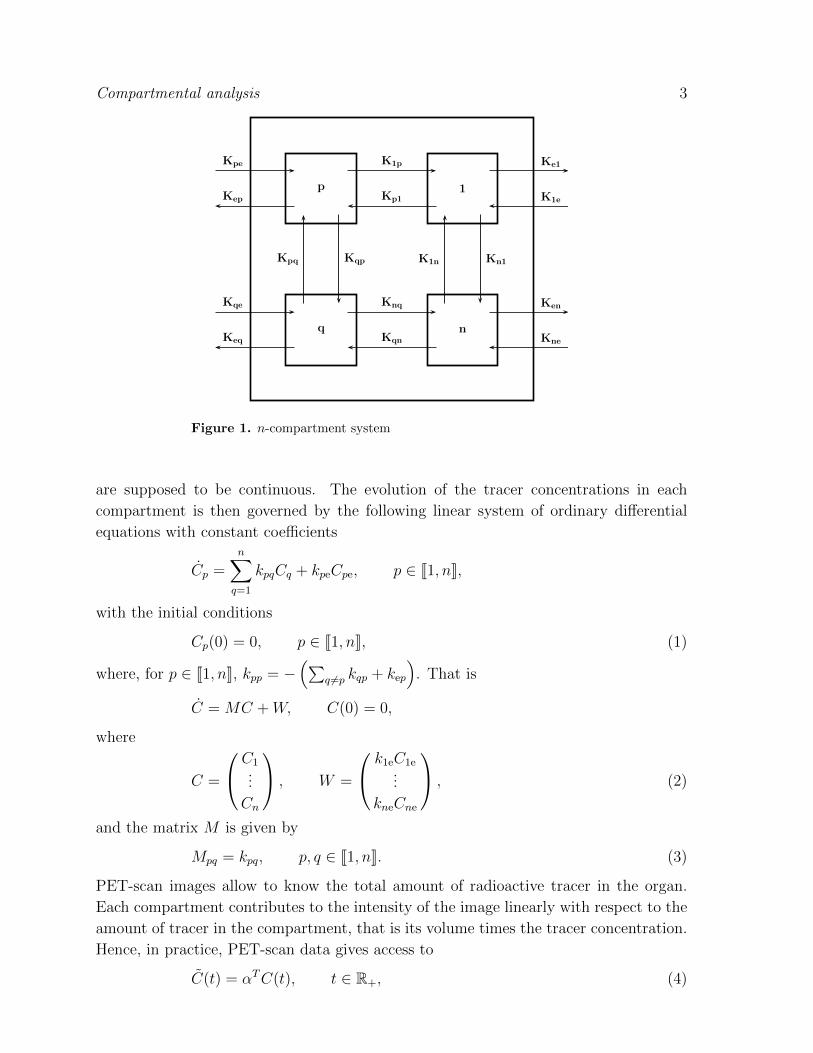
We consider a system composed of n compartments as in Figure 1, typically an
organ, where each compartment represents a functional behaviour of a tissue, or an
anatomical district. Remark that although the generic term “compartment” is used, it
does not necessary mean that each compartment is contained in a physical compartment
distinguishable from the others. In fact, this even constitutes one of the main issue in
the inverse problem of getting information on the system since each compartment can
not be individually observed. A radioactive tracer is injected to a patient and for a
compartment p ∈ J1, nK, Cp denotes the non-negative concentration function of the
tracer in the compartment. The compartment p receives the radioactive tracer from
the outside world at a constant non-negative rate kpe and a non-negative concentration
function Cpe and it excretes the tracer at a constant non-negative rate kep in the outside
world. The constant non-negative rate at which the compartment p receives the tracer
from a compartment q 6= p is denoted kpq. The concentration functions (Cpe)p∈J1,nK
Compartmental analysis 3
1p
q n
K1p
Kp1
Knq
Kqn
Kpq Kqp K1n Kn1
Kpe
Kep
Kqe
Keq
Ke1
K1e
Ken
Kne
Figure 1. n-compartment system
are supposed to be continuous. The evolution of the tracer concentrations in each
compartment is then governed by the following linear system of ordinary differential
equations with constant coefficients
Cp =n∑q=1
kpqCq + kpeCpe, p ∈ J1, nK,
with the initial conditions
Cp(0) = 0, p ∈ J1, nK, (1)
where, for p ∈ J1, nK, kpp = −(∑
q 6=p kqp + kep
). That is
C = MC +W, C(0) = 0,
where
C =
C1...
Cn
, W =
k1eC1e...
kneCne
, (2)
and the matrix M is given by
Mpq = kpq, p, q ∈ J1, nK. (3)
PET-scan images allow to know the total amount of radioactive tracer in the organ.
Each compartment contributes to the intensity of the image linearly with respect to the
amount of tracer in the compartment, that is its volume times the tracer concentration.
Hence, in practice, PET-scan data gives access to
C(t) = αTC(t), t ∈ R+, (4)
Compartmental analysis 4
where α ∈ R∗+n is a known constant vector. Thus, the inverse problem we consider is to
recover the exchange rates K ∈ Rn2+n, where
Kp =
kep, p ∈ J1, n2K, p ≡ 1 (mod n+ 1),
kp−nb p−1n c,1+b p−1
n c, p ∈ J1, n2K, p 6≡ 1 (mod n+ 1),
k(p−n2)e p ∈ Jn2 + 1, n2 + nK,
(5)
with measures of C. Note however that some exchange rates may be a priori known.
3. A Newton algorithm for the inverse problem
In the following of the document, for a positive integer n and K ∈ Rn2+n, we denote by
K ∈ Rn2the first n2 components of K and K ∈ Rn the last n components of K. For a
positive integer n, we denote by M the following linear operator
M : Rn2 → Mn(R)
H 7→ M(H),
where for all H ∈ Rn2
M(H)pq =
−H1+(n+1)(p−1) −
n∑p′ = 1p′ 6= p
Hp+n(p′−1), p, q ∈ J1, nK, p = q,
Hp+n(q−1), p, q ∈ J1, nK, p 6= q,
so that for all H ∈ Rn2
+ , M(H) is the matrix defined in (3) for the parameters H.
Consider now the linear operator Vec : Mn(R)→ Rn2stacking the columns of a matrix
A into a column vector Vec(A), that is
Vec(A)p = Ap−nb p−1n c,1+b p−1
n c, p ∈ J1, n2K. (6)
The operator VecM is linear from Rn2into itself, we denote by S ∈Mn2(R) its matrix.
It is a n2 × n2 sparse matrix with 2n2 − n non-zero elements which are equal to ±1.
More precisely, n2 − n entries of S are equal to 1 and n2 entries of S are equal to −1,
such as
Spq =
1, p, q ∈ J1, n2K, p = q, p 6≡ 1 (mod n+ 1),
−1, p, q ∈ J1, n2K, p ≡ 1 (mod n+ 1), p ≡ q (mod n),
0, otherwise.
(7)
We denote by W the following linear operator
W : C0(R+,R)n → L(Rn, C0(R+,R)n)
C 7→ W(C),
where for all C ∈ C0(R+,R)n, H ∈ Rn and p ∈ J1, nK, [W(C)(H)]p = HpCp, so that
for all vector of input concentrations functions C = (Cpe)p∈J1,nK ∈ C0(R+,R+)n and
Compartmental analysis 5
H ∈ Rn+, W(C)(H) is the vector defined in (2) for the input concentrations functions C
and the parameters H. We denote by C the following function
C : C0(R+,R)n → L(Rn2+n, C1(R+,R)n)
C 7→ C(C),
where for all C ∈ C0(R+,R)n and K ∈ Rn2+n, C = C(C)(K) ∈ C1(R+,R)n is the
unique solution to
C = MC +W, C(0) = 0,
where M = M(K) and W = W(C)(K). For α ∈ R∗+n, Cα is the function defined by
Cα : C0(R+,R)n → L(Rn2+n, C1(R+,R))
C 7→[K 7→ αT (C(C)(K))
].
3.1. Algorithm description
We consider a n-compartment system as in Figure 1 with known input concentration
functions C = (Cpe)p∈J1,nK ∈ C0(R+,R+)n and α ∈ R∗+n. We recall that the problem we
are interested in consists in recovering the exchange rates K ∈ Ω ⊂ Rn2+n, where K is
given by (5), from the knowledge of C(K), where C = Cα(C). We recall that
C(K)(t) = αTC(K)(t), t ∈ R+,
where C = C(C). The concentrations vector C(K) is the solution of the ordinary
differential equations
C(K) = M(K)C(K) +W (K), C(K)(0) = 0,
where W = W(C). The solution C(K) to the system of ordinary differential equations
is given by
C(K)(t) =
∫ t
0
exp((t− τ)M(K))W (K)(τ) dτ, t ∈ R+,
hence
C(K)(t) = αT∫ t
0
exp((t− τ)M(K))W (K)(τ) dτ, t ∈ R+.
C : Rn2+n → C1(R+,R)n can be easily seen to be differentiable and even analytic. In
order to use a Newton algorithm, we need to compute its Frechet derivative. More
precisely, considering t ∈ R+, we will compute the gradient of Ct for all t ∈ R+, with
respect to K, where for all K ∈ Rn2+n, Ct(K) = C(K)(t). For all K ∈ Rn2+n, the
Frechet derivative dCdK
(K) of C at K, bounded operator from Rn2+n to C1(R+,R) is
then given by
dC
dK(K) : Rn2+n → C1(R+,R),
H 7→[t 7→ ∇Ct(K) ·H
].

Compartmental analysis 6
For all t ∈ R+, the gradient of Ct is given by
∇Ct =
(∇KCt∇KCt
), (8)
where ∇K denotes the gradient with respect to K and ∇K denotes the gradient with
respect to K. Since Ct is linear with respect to K, we simply have for all K ∈ Rn2+n
∇KCt(K) =
(∫ t
0
C(τ) exp((t− τ)M(K)T ) dτ
)α, (9)
where denotes the Khatri-Rao product. Compute now the gradient of Ct with respect
to K. Writing Ct as
Ct(K) = αTFt(K,M(K)), K ∈ Rn2+n,
where for all K ∈ Rn2+n and N ∈Mn(R)
Ft(K,N) =
∫ t
0
exp((t− s)N)W (K)(s) ds,
we have for all K ∈ Ω and N,H ∈ Rn2
∇KCt(K) ·H = αT∂Ft∂N
((K,M(K)
);dM
dK(K;H)
),
and since M : Rn2 →Mn(R) is linear
∇KCt(K) ·H = αT∂Ft∂N
((K,M(K)
);M(H)
). (10)
Hence, to compute the gradient of Ct with respect to K, we need to compute the Frechet
derivative of Ft with respect to the second variable N ∈Mn(R). The Frechet derivative
of the exponential function can be written in this way
d exp
dN(N ;H) =
∫ 1
0
exp(τN)H exp((1− τ)N) dτ, N,H ∈Mn(R).
Hence, for all K ∈ Ω and N,H ∈Mn(R)
∂Ft∂N
((K,N
);H)
=
∫ t
0
(t− s)(∫ 1
0
exp(τ(t− s)N)H exp((1− τ)(t− s)N) dτ
)W (K)(s) ds,
that is, with the change of variables τ(t− s)→ τ
∂Ft∂N
((K,N
);H)
=
∫ t
0
(∫ t−s
0
exp(τN)H exp((t− s− τ)N) dτ
)W (K)(s) ds.
Hence
∂Ft∂N
((K,N
);H)
=
∫ t
0
(∫ t−τ
0
exp(τN)H exp((t− s− τ)N)W (K)(s) ds
)dτ,
so that making the change of variables (t− τ)→ τ , we get
∂Ft∂N
((K,N
);H)
=
∫ t
0
exp((t− τ)N)H
(∫ τ
0
exp((τ − s)N)W (K)(s) ds
)dτ.
Compartmental analysis 7
In other words
∂Ft∂N
((K,N
);H)
=
∫ t
0
exp((t− τ)N)HFτ (N) dτ.
Writing the previous formula in a more convenient way for computations, we have
∂Ft∂N
((K,N
);H)
=
(∫ t
0
Fτ (N)T ⊗ exp((t− τ)N) dτ
)Vec(H),
where ⊗ denotes the Kronecker product and the linear operator Vec : Mn(R) → Rn2,
stacking the column of a matrix into a column vector, is defined in (6). Consequently,
from (10), we have for all K ∈ Rn2+n and H ∈ Rn2
∇KCt(K) ·H = αT(∫ t
0
C(K)(τ)T ⊗ exp((t− τ)M(K)) dτ
)Vec(M(H)).
Recalling that S, defined in (7), denotes the matrix of the linear operator Vec M :
Rn2 → Rn2, we then have
∇KCt(K) ·H = αT(∫ t
0
C(K)(τ)T ⊗ exp((t− τ)M(K)) dτ
)SH,
so that
∇KCt(K) = ST(∫ t
0
C(K)(τ)⊗ exp((t− τ)M(K)T ) dτ
)α. (11)
Hence, using (8), (9), (11)
∇Ct(K) =
∫t
0
(ST(C(K)(τ)⊗ exp((t− τ)M(K)T )
)α(
C(τ) exp((t− τ)M(K)T ))α
)dτ.
In other words, for all K,H ∈ Rn2+n and t ∈ R+, we have[dC
dK(K;H)
](t) =
∫
t
0
(ST(C(K)(τ)⊗ exp((t− τ)M(K)T )
)α(
C(τ) exp((t− τ)M(K)T ))α
)dτ
H.
Consider a known function Cmeas ∈ C1(R+,R), the measures of C(Kexact) where Kexact
are the real unknown exchange rates of the compartmental system. Let K0 ∈ Ω be
an initial guess, then the Newton algorithm consists in solving the linear equation with
unknown H0 ∈ Ω[dC
dK(K0;H0)
](t) = Cmeas(t)− C(K0)(t), for all t ∈ R+. (12)
Then, increment the value K0, giving K1 = K0 +H0 and iterate the process.
Compartmental analysis 8
3.2. Implementation details
The equation (12) may have no solution, moreover, in real applications, one has only
the measured data Cmeas for a finite number of sampling time points t1, . . . , tm ∈ R+
and the data may be noisy. The discretized Newton algorithm consists in solving the
linear system (12) by Tikhonov regularization. The non-regularized discretized system
is given by [∇Ct1(K0)
]T...[
∇Ctm(K0)]TH0 =
Cmeas(t1)− Ct1(K0)...
Cmeas(tm)− Ctm(K0)
,
that is, denoting by A0 the matrix
A0 =
[∇Ct1(K0)
]T...[
∇Ctm(K0)]T ,
and by Y 0 the vector
Y 0 =
Cmeas(t1)− Ct1(K0)...
Cmeas(tm)− Ctm(K0)
,
the non-regularized discretized system can be written as
A0H0 = Y 0. (13)
Solving the system (13) by Tikhonov regularization consists in finding the solution H0
to
(rI + AT0A0)H0 = AT0 Y0,
where r is a regularization parameter. As previously described, the value K0 is
incremented, giving K1 = K0 + H0 and the process is iterated. Note that the
regularization parameter can be different at each iteration step.

Compartmental analysis 9
4. The FDG–PET models
Figure 2. 2-compartment catenary model
As already mentioned, FDG is largely used for PET, mainly in the case of oncological
applications. In fact, FDG-PET is based on the higher glycolytic activity in tumor
cells compared to healthy tissue as the cause of image contrast. This glucose–analog
behaviour implies that FDG is transported into malignant cells, which therefore exhibit
increased radioactivity. From a biochemical viewpoint, FDG may follow a two-destiny
path: in the first path FDG molecules are phosphorylated by means of a 6-phosphate
group and remain trapped within the cells while, in the second path, FDG is not
metabolized and therefore remains free in the tissue. This behaviour implies that,
from a compartmental perspective, the analysis of FDG-PET data relies on a model
made of an Input Function (in general, but not exclusively, an arterial one) and two
functional compartments describing the free tracer and the trapped, metabolized FDG-
6P, respectively.
In the two-compartment model of FDG-PET data (see Figure 2) the state variables
are the tracer concentration in compartments Cf and Cm for the free and metabolized
compartments, respectively, while the kinetic process in the system is initialized by
the Input Function (IF) Cb, representing the tracer concentration in blood. The
four constant transmission coefficients between the communicating compartments are
denoted, for sake of simplicity, as k1, k2, k3, k4. The model equations for the forward
and inverse problem are easily obtained from the general form in eq (1)–(5).
Next subsections describe three compartmental models for the FDG related to
different physiological systems.
4.1. The model of the brain
For the FDG model of the brain, we will use a two–compartment catenary
compartmental model. Indeed, even if from a functional (neuronal) viewpoint the brain
has an extremely complex behaviour, brain–glucose metabolism inside the brain can
Compartmental analysis 10
be thought as standard [15]. We are aware that recently has been shown that the
brain exchange coefficients of the compartmental systems, can vary very much according
to the spatial position in the organ. For this reason, the two–compartment catenary
compartmental system used for describing the brain physiology is modelled, applied and
reduced pixelwise [16, 17, 18]. Such compartmental models are known as parametric
compartmental models or indirect parametric imaging.
We will not discuss such parametric models, and otherwise discuss the validity and
robustness of our technique if applied to a two–compartment system, using brain data
to validate it on real imaging FDG–PET data.
4.2. The model of the liver
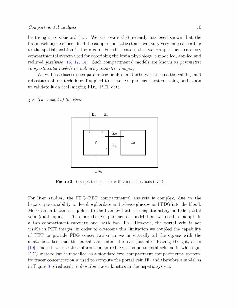
Figure 3. 2-compartment model with 2 input functions (liver)
For liver studies, the FDG–PET compartmental analysis is complex, due to the
hepatocyte capability to de–phosphorilate and release glucose and FDG into the blood.
Moreover, a tracer is supplied to the liver by both the hepatic artery and the portal
vein (dual input). Therefore the compartmental model that we need to adopt, is
a two–compartment catenary one, with two IFs. However, the portal vein is not
visible in PET images; in order to overcome this limitation we coupled the capability
of PET to provide FDG concentration curves in virtually all the organs with the
anatomical ken that the portal vein enters the liver just after leaving the gut, as in
[19]. Indeed, we use this information to reduce a compartmental scheme in which gut
FDG metabolism is modelled as a standard two–compartment compartmental system,
its tracer concentration is used to compute the portal vein IF, and therefore a model as
in Figure 3 is reduced, to describe tracer kinetics in the hepatic system.
Compartmental analysis 11
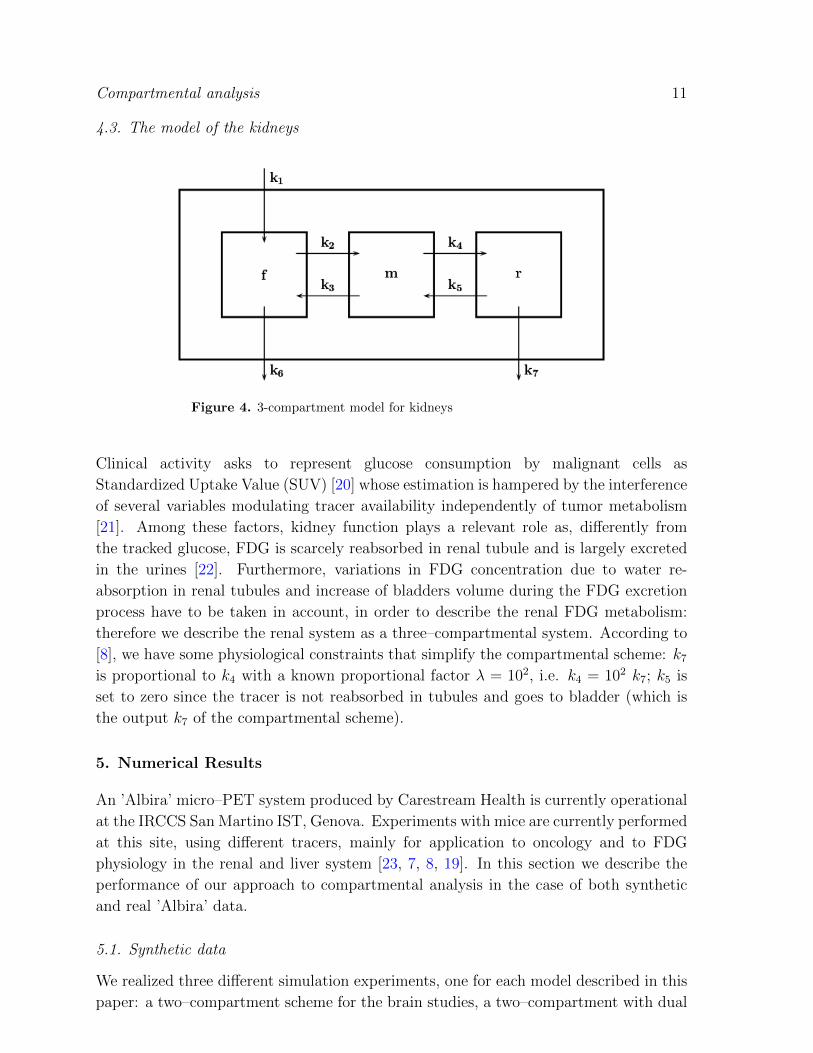
4.3. The model of the kidneys
Figure 4. 3-compartment model for kidneys
Clinical activity asks to represent glucose consumption by malignant cells as
Standardized Uptake Value (SUV) [20] whose estimation is hampered by the interference
of several variables modulating tracer availability independently of tumor metabolism
[21]. Among these factors, kidney function plays a relevant role as, differently from
the tracked glucose, FDG is scarcely reabsorbed in renal tubule and is largely excreted
in the urines [22]. Furthermore, variations in FDG concentration due to water re-
absorption in renal tubules and increase of bladders volume during the FDG excretion
process have to be taken in account, in order to describe the renal FDG metabolism:
therefore we describe the renal system as a three–compartmental system. According to
[8], we have some physiological constraints that simplify the compartmental scheme: k7
is proportional to k4 with a known proportional factor λ = 102, i.e. k4 = 102 k7; k5 is
set to zero since the tracer is not reabsorbed in tubules and goes to bladder (which is
the output k7 of the compartmental scheme).
5. Numerical Results
An ’Albira’ micro–PET system produced by Carestream Health is currently operational
at the IRCCS San Martino IST, Genova. Experiments with mice are currently performed
at this site, using different tracers, mainly for application to oncology and to FDG
physiology in the renal and liver system [23, 7, 8, 19]. In this section we describe the
performance of our approach to compartmental analysis in the case of both synthetic
and real ’Albira’ data.
5.1. Synthetic data
We realized three different simulation experiments, one for each model described in this
paper: a two–compartment scheme for the brain studies, a two–compartment with dual

Compartmental analysis 12
BRAIN k1 k2 k3 k4
g. t. 1.00 0.20 0.05 0.80
MGN 1.05± 0.04 0.20± 0.02 0.05± 0.01 0.82± 0.03
LS 1.02± 0.08 0.18± 0.05 0.05± 0.05 0.80± 0.03
Table 1. Validation with a synthetic dataset: ground–truth (g.t.) values of the
tracer coefficients compared with the reconstructions provided by multilinear fitting
with the Levenberg-Marquardt Least-Squares algorithm (LS) and by our regularized
Multivariate Gauss Newton (MGN) approach. V is set equal to 0.02.
input model for the liver (coupled with a standard two–compartment scheme for the
gut) and a three compartment model for renal studies.
In order to produce the synthetic data we initially chose realistic values for V (the
blood fraction that supplies the organ of interest) and for λ of the renal system; then
we utilized ground truth (g.t.) values for all the tracer kinetic parameters (4 in the
brain case, 4+4 in the gut–liver case and 5 in the kidneys case). With these selected
values we solved every forward problems (1)–(3) in term of C. These solutions of the
Cauchy problems are sampled in time, on a total interval [t1, tm] that corresponds to
the total acquisition time with ’Albira’ and in correspondance of time points typical of
experiments with the scanner in this application context. The Input Function Cb has
always been obtained by fitting with a gamma variate function a set of real measurements
acquired from a healthy mouse in a very controlled experiment [24]. We computed the
data C as in (4), affected the data by Poisson noise, and applied our algorithm in
order to reconstruct the exchange coefficients. The Tikhonov regularization parameter
r was optimized at each iteration using the Generalized Cross Validation technique [25].
Comparison with the g.t. values for this parameters provides limits about the reliability
of the model and of the inversion procedure.
The results of this test are given in Tables 1, 2 and 3, where mean and standard
deviations are computed over 50 runs of the same problem with different (random)
initialization vectors K(0), in a Monte Carlo approach. Iterations are stopped with a
discrepancy principle on data in combination with a tolerance on the step–size H of
the Newton Method. The computational burden is ' 10 seconds for each Monte Carlo
run (on a Intel i5 2.3GHz x 4). In Tables, we show also comparison with a standard
Levemberg–Marquardt method for the least–squares minimization [26]. Comparison
with respect to the ground–truth values and the values provided by the Levenberg-
Marquardt method, and the small values for the reconstruction uncertainties clearly
show the reliability of our approach.
5.2. Real FDG–PET data
For our experiment we consider a control group (n=10) and a group (of the same size) in
which FDG injection was performed after one month of high dose metformin treatment

Compartmental analysis 13
GUT–LIVER kG1 kG2 kG3 kG4 (= kv) ka k2 k3 k4g. t. 1.00 0.20 0.10 1.00 1.50 0.40 0.30 0.60
MGN 1.03± 0.03 0.19± 0.2 0.10± 0.01 0.99± 0.02 1.52± 0.04 0.41± 0.03 0.29± 0.02 0.59± 0.01LS 1.01± 0.07 0.23± 0.4 0.10± 0.07 1.00± 0.10 1.51± 0.12 0.39± 0.06 0.29± 0.04 0.60± 0.07
Table 2. Validation with a synthetic dataset: ground–truth (g.t.) values of the
tracer coefficients compared with the reconstructions provided by multilinear fitting
with the Levenberg-Marquardt Least-Squares algorithm (LS) and by our regularized
Multivariate Gauss Newton (MGN) approach. Simulated values of tracer coefficients,
and reconstructed values for both the gut (kGi ) and the liver coefficients. V for the
liver is set equal to 0.3; V for the gut is set equal to 0.1.
KIDNEYS k1 k2 k3 k4 k6
g. t. 0.80 0.10 0.20 1.00 0.70
MGN 0.81± 0.03 0.11± 0.01 0.20± 0.03 1.02± 0.02 0.72± 0.03
LS 0.80± 0.10 0.09± 0.03 0.21± 0.05 1.00± 0.11 0.70± 0.09
Table 3. Validation with a synthetic dataset: ground–truth (g.t.) values of the
tracer coefficients compared with the reconstructions provided by multilinear fitting
with the Levenberg-Marquardt Least-Squares algorithm (LS) and by our regularized
Multivariate Gauss Newton (MGN) approach. V is set equal to 0.3, and the
proportional factor λ is 102 (such that k7 = 1λk4).
(750 mg/Kg body weight daily). This drug reduces blood glucose concentration without
causing hypoglycemia [27], mostly by decreasing intestinal glucose absorption and
glucose delivery by the liver [23]. It follows that nuclear medicine experiments with
such kind of animal models are perfect candidates to validate a compartmental model
that has been designed in order to follow the FDG kinetics in the hepatic and renal
system in a refined fashion [8, 19].
To ensure a steady state of substrate and hormones governing glucose metabolism,
the small animal was studied after six hours fasting. Mouse was weighted and
anaesthesia was induced by intra-peritoneal administration of ketamine/xylazine (100
and 10 mg/kg, respectively). Serum glucose level was tested and animals were positioned
on the bed of the scanner, whose two–ring configuration permits to cover the whole
animal body in a single bed position. The mouse was injected with a dose of 3–4 MBq of
FDG through a tail vein soon after the start of a list mode acquisition lasting 50 minutes.
Acquisition was performed using the following framing rate: 10 × 15 sec, 5 × 30 sec, 2
× 150 sec, 6 × 300 sec, 1 × 600 sec. PET data were reconstructed using a Maximum
Likelihood Expectation Maximization method (MLEM) [28]. Thereafter, each image
dataset was reviewed by an experienced observer who recognized five Regions Of Interest
(ROIs) encompassing left ventricle, brain, gut and liver and kidneys respectively (as in
Figure 5). The ROIs over the left ventricle allowed us to compute the IF (we are aware
that the determination of IF is a challenging task in the case of mice. To accomplish
it, for each animal model we have first viewed the tracer first pass in cine mode; then,
in a frame where the left ventricle was particularly visible, we have drawn a ROI in
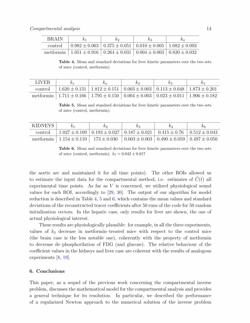
Compartmental analysis 14
BRAIN k1 k2 k3 k4
control 0.982± 0.063 0.375± 0.051 0.010± 0.005 1.082± 0.093
metformin 1.051± 0.916 0.264± 0.031 0.004± 0.003 0.820± 0.032
Table 4. Mean and standard deviations for liver kinetic parameters over the two sets
of mice (control, metformin).
LIVER kv ka k2 k3 k4
control 1.620± 0.131 1.812± 0.151 0.003± 0.003 0.113± 0.048 1.873± 0.201
metformin 1.711± 0.166 1.795± 0.150 0.004± 0.003 0.023± 0.011 1.906± 0.182
Table 5. Mean and standard deviations for liver kinetic parameters over the two sets
of mice (control, metformin).
KIDNEYS k1 k2 k3 k4 k6
control 1.027± 0.109 0.193± 0.027 0.187± 0.021 0.415± 0.76 0.512± 0.043
metformin 1.154± 0.110 173± 0.030 0.003± 0.003 0.490± 0.059 0.497± 0.050
Table 6. Mean and standard deviations for liver kinetic parameters over the two sets
of mice (control, metformin). k7 = 0.042± 0.017
the aortic arc and maintained it for all time points). The other ROIs allowed us
to estimate the input data for the compartmental method, i.e. estimates of C(t) all
experimental time points. As far as V is concerned, we utilized physiological sound
values for each ROI, accordingly to [29, 30]. The output of our algorithm for model
reduction is described in Table 4, 5 and 6, which contains the mean values and standard
deviations of the reconstructed tracer coefficients after 50 runs of the code for 50 random
initialization vectors. In the hepatic case, only results for liver are shown, the one of
actual physiological interest.
These results are physiologically plausible: for example, in all the three experiments,
values of k3 decrease in metformin–treated mice with respect to the control mice
(the brain case is the less notable one), coherently with the property of metformin
to decrease de–phosphorilation of FDG (and glucose). The relative behaviour of the
coefficient values in the kidneys and liver case are coherent with the results of analogous
experiments [8, 19].
6. Conclusions
This paper, as a sequel of the previous work concerning the compartmental inverse
problem, discusses the mathematical model for the compartmental analysis and provides
a general technique for its resolution. In particular, we described the performance
of a regularized Newton approach to the numerical solution of the inverse problem
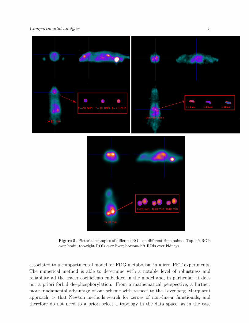
Compartmental analysis 15
Figure 5. Pictorial examples of different ROIs on different time points. Top-left ROIs
over brain; top-right ROIs over liver; bottom-left ROIs over kidneys.
associated to a compartmental model for FDG metabolism in micro–PET experiments.
The numerical method is able to determine with a notable level of robustness and
reliability all the tracer coefficients embedded in the model and, in particular, it does
not a priori forbid de–phosphorylation. From a mathematical perspective, a further,
more fundamental advantage of our scheme with respect to the Levenberg–Marquardt
approach, is that Newton methods search for zeroes of non–linear functionals, and
therefore do not need to a priori select a topology in the data space, as in the case

Compartmental analysis 16
of least–squares approaches. Results on real data verify the reliability of the method in
estimating physiologically sound values for the tracer coefficients, that are in agreement
with literature.
A Matlab prototype implementing this approach is at disposal at together with a
Graphical User Interface for user-friendly input/output processing.
References
[1] Ollinger J M and Fessler J A 1997 IEEE Signal Processing Magazine 14 43–55
[2] Antoch G, Saoudi N, Kuehl H, Dahmen G, Mueller S P, Beyer T, Bockisch A, Debatin J F and
Freudenberg L S 2004 Journal of Clinical Oncology 22 4357–4368
[3] Avril N, Menzel M, Dose J, Schelling M, Weber W, Janicke F, Nathrath W and Schwaiger M 2001
Journal of Nuclear Medicine 42 9–16
[4] Ziegler W A W S I, Thodtmann R, Hanauske A R and Schwaiger M 1999 J Nucl Med 40 1771–1777
[5] Delbeke D, Coleman R E, Guiberteau M J, Brown M L, Royal H D, Siegel B A, Townsend D W,
Berland L L, Parker J A, Hubner K et al. 2006 Journal of Nuclear Medicine 47 885–895
[6] Engl H W, Hanke M and Neubauer A 1996 Regularization of inverse problems vol 375 (Springer
Science & Business Media)
[7] Garbarino S, Caviglia G, Brignone M, Massollo M, Sambuceti G and Piana M 2013 Computational
and mathematical methods in medicine 2013
[8] Garbarino S, Caviglia G, Sambuceti G, Benvenuto F and Piana M 2014 Physics in medicine and
biology 59 2469
[9] Gunn R N, Gunn S R and Cunningham V J 2001 Journal of Cerebral Blood Flow & Metabolism
21 635–652
[10] Kamasak M E, Bouman C A, Morris E D and Sauer K 2005 Medical Imaging, IEEE Transactions
on 24 636–650
[11] Qiao H, Bai J, Chen Y and Tian J 2007 International journal of biomedical imaging 2007
[12] Schmidt K and Turkheimer F 2002 The Quarterly Journal of Nuclear Medicine and Molecular
Imaging 46 70
[13] Sourbron S and Buckley D L 2011 Physics in medicine and biology 57 R1
[14] Delbary F, Garbarino S and Vivaldi V Inverse problems, submitted
[15] Alf M F, Wyss M T, Buck A, Weber B, Schibli R and Kramer S D 2013 Journal of Nuclear
Medicine 54 132–138
[16] Karakatsanis N A, Lodge M A, Zhou Y, Wahl R L and Rahmim A 2013 Physics in medicine and
biology 58 7419
[17] Wardak M, Schiepers C, Wong K P and Huang S C 2013 Simplified reference tissue models for
kinetic analysis of dynamic flt pet imaging in patients undergoing brain tumor treatment Society
of Nuclear Medicine Annual Meeting Abstracts vol 54 (Soc Nuclear Med) p 1415
[18] Angelis G I, Matthews J C, Kotasidis F A, Markiewicz P J, Lionheart W R and Reader A J 2014
Annals of nuclear medicine 28 860–873
[19] Garbarino S, Vivaldi V, Delbary F, Caviglia G, Piana M, Marini C, Capitanio S, Calamia I,
Buschiazzo A and Sambuceti G 2015 EJNMMI Research 5 1
[20] Delbeke D, Rose D M, Chapman W C, Pinson C W, Wright J K, Shyr R D B Y and Leach S D
1999 J Nucl Med 40 1784–1791
[21] Diederichs C G, Staib L, Glatting G, Beger H G and Reske S N 1998 The Journal of Nuclear
Medicine 39 1030
[22] Shreve P D, Anzai Y and Wahl R L 1999 Radiographics 19 61–77
[23] Massollo M, Marini C, Brignone M, Emionite L, Salani B, Riondato M, Capitanio S, Fiz F,
Democrito A, Amaro A et al. 2013 Journal of Nuclear Medicine 54 259–266

Compartmental analysis 17
[24] Golish S R, Hove J D, Schelbert H R and Gambhir S S 2001 Journal of Nuclear Medicine 42
924–931
[25] Golub G H, Heath M and Wahba G 1979 Technometrics 21 215–223
[26] Nocedal J and Wright S 2006 Numerical optimization (Springer Science & Business Media)
[27] Klepser T and Kelly M 1997 American journal of health-system pharmacy 54 893–903
[28] Hudson H M and Larkin R S 1994 Medical Imaging, IEEE Transactions on 13 601–609
[29] Keiding S 2012 Journal of Nuclear Medicine 53 425–433
[30] Marzola P, Farace P, Calderan L, Crescimanno C, Lunati E, Nicolato E, Benati D, Degrassi A,
Terron A, Klapwijk J et al. 2003 International journal of cancer 104 462–468