www.efv.admin.ch

Application of the Swiss Fiscal Rule to Artifi cial Data

Working Paper No. 5 EFVEFV

The work of the FFA group of economic advisors does not necessarily refl ect the offi cial position of the offi ce or federal department or that of the Fe-deral Council. The authors themselves are respon-sible for the assumptions and any errors which may be contained in the work.

Impressum

RedaktionEidg. FinanzverwaltungAutor: Alain Geier

Layout: U. Gmür

ISSN-Nr. 1660-7937

Bern, Oktober 2004

Internet:www.efv.admin.ch/d/wirtsch/studien/berichte.htm

3

Abstract

The present notice applies the Swiss fi scal rule or «debt brake» to simulated data of economic output and fi scal revenues. It appears that the budget remains almost perfectly balanced in the medium and long term a the debt ratio does neither decrease nor increase in excess of a few points of GDP over the medium and long term. This approach therefore represents an additional indication that the debt brake is effective in terms of its primary objective of achieving a balanced budget over the medium term. The rule also performs adequately well with respect to the secondary objective of taking into account the business cycle position. In this simulation the policy stance was fairly adequate. Cases of pro-cyclical policy occur mainly near a closed output gap with a budget close to equilibrium.

5

Contents

1 Introduction 7

2 Theory of the debt brake 9

3 Simulation 10

3.1. Sinusoidal business cycles 11

3.2. Random business cycles 12

3.3. Random walk with drift 15

3.4. General remarks 15

4 Results 18

5 Conclusion 21

Literature 22

Appendix 1 : Simulation results 23

Appendix 2 : Fiscal policy stance 24

Appendix 3 : Adjustment account 25

Veröffentlichte „Working papers“ des Ökonomenteams EFV 26

7

In the context of recent discussions (such as Müller, 2003) about the Swiss Confederation’s fi scal rule —or «debt brake»1— some concerns were raised about its ability to balance the budget over the medium term. As this objective is an explicit requirement of the Federal Constitution, the question should be addressed. The present paper is one possible approach to fi nd an answer to this question. It uses long series of artifi cial data to illustrate the behaviour of the fi scal rule in the long term and test whether the objective of a balanced budget can be met. Other approaches might include a simulation on actual historical data, like Geier (2003), or the formal derivation of the rule’s properties, like Bruchez (2003a).

Given the presence of various uncertainties that accompany every budgetary process, and the fact that planned revenues and expendi-tures can change throughout the budgeted fi scal year, it seems plau-sible to imagine that the fi scal rule can only approximately balance a budget. Hence the relevant question should be whether a balanced budget can be reached within a limit of tolerance or if there are some systematic biases toward either defi cits or surpluses. The an-swer to this question must be completed by taking into account the working of the adjustment account, which is an important feature of the debt brake2. One of its functions consists precisely in ruling out systematic biases. Minor fl aws in the design can be eliminated this

1 Introduction

1 the mechanism is described in the accompanying message of the Federal Council to the amendment of the budget legislation: Botschaft zur Schuldenbremse vom 05.07.2000, Schweizer Bundesrat.2 a description of the adjustment account can be found in Bodmer (2003), in the Botschaft zur Schuldenbremse and regarding recent modifi cations to its calculation in the Botschaft zum Entlastungsprogramm 2003.

8

way. The problem therefore boils down to knowing whether re-maining biases and deviations from a perfectly balanced budget are small enough for the adjustment account to eliminate them without disrupting the budgetary process.

The present paper simulates the behaviour of the debt brake ap-plied to a modelled GDP series and tests whether budget balance is achieved in the medium term and whether debt remains within fi xed limits. After describing the Swiss debt brake (§2), we will present our simulations (§3) and results (§4). Section 5 will propose concluding remarks.

9

The debt brake formula:

with

states that for any moment of calculation (t) the maximum allowed expenditures ( ) must equal (budgeted) revenues (T), after multi-plication with the «business cycle adjustment factor» or k-factor (k). The factor k aims at stabilising expenditures around the level of cycli-cally adjusted revenues, and consists of the ratio of trend real output (Y*) and actual (real) output (Y). The proof that this formula will yield a balanced budget is not straightforward. It depends notably on the assumption that the expected value of the right hand side of equa-tion (1) ( kT ) is equal to the expected value of revenues (T) over the long run. If k and T were independent random variables the proof would be easier to establish. However, they are clearly negatively correlated as both depend in opposite ways on the real output of the economy. An automatically balanced budget is therefore not an in-tuitively necessary outcome. A further complication is introduced by a positive trend in economic growth. The consequence of this is that two consecutive business cycles do not have the same amplitude. On the other hand, economic growth tends to reduce past errors over time if the budget balance and debt are expressed in terms of GDP, since past deviations become more and more insignifi cant. More importantly, the way that revenues are forecasted probably plays an important role. However, detecting possible biases in the forecasting methods is not the purpose of these simulations. The reader will fi nd a discussion in Bodmer (2003a).

2 Theory of the debt brake

(1)

10

The present work simulates the behaviour of the debt brake ap-plied to a modelled GDP series and test whether budget balance is achieved in the medium term and whether debt remains within fi xed limits. The relevant measure for both shall not be absolute values of budget defi cits and debt, but the ratio of these fi gures with respect to GDP. As GDP is subject to a growth trend, all related variables will grow at the same pace. Therefore these values are not stationary. Taking the ratio with respect to GDP also makes values comparable for different time periods. We will consider that the budget is bal-anced if this ratio is on average close to zero.

Some attention is also given to the factor k. If the expected value of k equals one, this means, according to (3.1) that the expected value of expenditures in terms of revenues is also one. This statement does not necessarily imply a balanced budget, but it is a strong indication that the balanced budget requirement can be met.

This section analyses the effect of simulated data based on (a) sinu-soidal business cycles, (b) business cycles of variable length and (c) a random walk (with drift). The cases (b) and (c) add a complication for the statistical fi lter which is designed for specifi c periods and may show different features for different periodicities. It is therefore inter-esting to simulate the impact of a change in the period of business cycles. It can be assumed that a longer period will result in the statis-tical fi lter underestimating the cyclical component. However, from a point of view of a balanced budget this may seem desirable even if a perfectly correct representation of the output gap may thus become more diffi cult. The random walk scenario puts the test to the limit. As there are no business cycles in this scenario, the main interest in this case is to test whether the budget still remains balanced.

3 Simulation

11

3.1. Sinusoidal business cycles

The idea of this scenario is to generate a growing GDP, superseded with a cyclical component. The structural component Ys is growing at a constant rate g:

The cyclical component Yc is the structural component Ys multiplied with a sinusoidal function. Using (3.1) it can be expressed in terms of

alone:

which allows a simple expression for GDP:

(3.1)

(3.2)

12

and therefore

The parameters of this model are calibrated to meet the Swiss GDP’s estimated trend growth of around 2%, its standard deviation of also around 2%, the typical length of a business cycle (6-7 years) and the typical standard deviation of the output gap which amounts to around 2%3. This yields:

3.2. Random business cycles

This model follows an idea similar to the previous case. The differ-ence is that the cyclical component is not sinusoidal, but its length and its amplitude are random. Equations (3.4) and (3.1) also apply in this case:

The cyclical component is less straightforward, but the numerical simulation resulting from it can be achieved quite easily. The cyclical

3 It comes as no surprise that this value is close to the standard deviation of growth.

35 0.02.

(3.1)

(3.3)

(3.4)

13

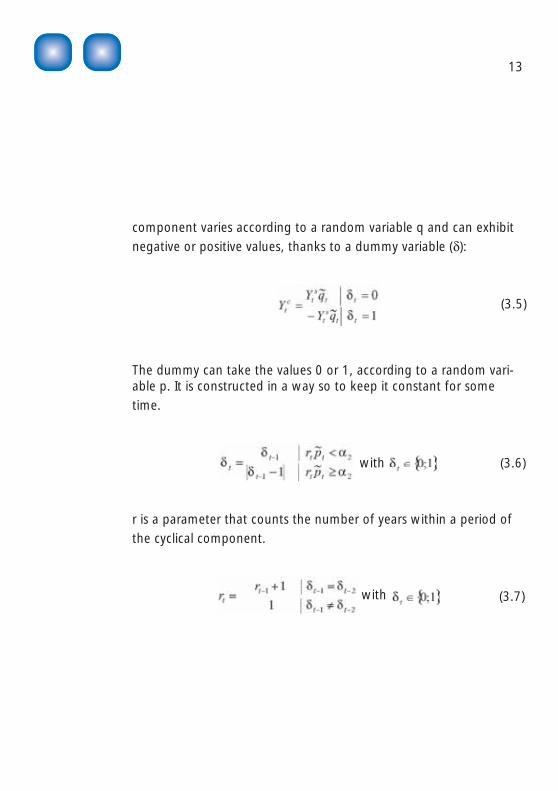
component varies according to a random variable q and can exhibit negative or positive values, thanks to a dummy variable (δ):

The dummy can take the values 0 or 1, according to a random vari-able p. It is constructed in a way so to keep it constant for some time.

r is a parameter that counts the number of years within a period of the cyclical component.

(3.7)

(3.6)

(3.5)

with

with

14

There are positive and negative periods. Two adjacent periods form a business cycle.

p and follow a uniform distribution:

uniform distribution [0;1]

Again, the parameters are calibrated to conform to the expected output gap, economic growth rate, its standard deviation and the length of a business cycle of 6-7 years. The length of half a business cycle (above trend or below trend) varies between the extreme val-ues of two and nine years. A business cycle lasts 6.8 year on average with a standard deviation of 2.3 years. This is achieved by setting the different parameters:a2 = 0.015, a3 = 30, g = 0.02.

(3.8)

15

3.3. Random walk with drift

This scenario is a straightforward random walk with drift model:

(3.9)

(3.10)

(3.11)

with std.normal distribution N (0;1)

One important feature is that it does not include a specifi cally cyclical component. Again, the model is calibrated to meet expected proper-

ties of GDP growth with 0.02 and 0.02

3.4. General remarks

The sample has a length of 10’000 periods. The fi scal revenue series have an additional overlay of a random or «irregular» variable, which should simulate its imperfect relation to GDP as is observed in the real world. The extent of this random component corresponds roughly to the observed magnitude of the irregular component of the Confederation’s revenues as it is described by Bodmer and Geier (2003).

16

Fiscal revenues are modelled the following way:

The operational defi nition of T is:

The irregular component is a random proportion to actual revenue:

with std.normal distribution N (0;1)

We assume that Tt is perfectly known at time t. A modelling of revenue forecasts is not the purpose of this paper. The conclusions of this paper should not be affected to the worse by this assumption, as revenue estimates seem to be unbiased and errors seem to favour a more anti-cyclical behaviour of the rule4.

The k-factors are calculated on effective structural values (theoretical value) as well as on trend values using a modifi ed Hodrick Prescott-fi lter5 applied recursively (calculated value). Recursively here means that each trend value is a value at the end of a rolling sample. The

4 see for instance Bodmer (2004)

(3.12)

(3.13)

(3.14)

17

length of the rolling sample is 23 periods, the same as the value used by the Federal Finance Administration for the actual calculation of the k-factor. The fi lter is applied exclusively to logarithms of GDP.

The factor k is calculated according to both true values and esti-mated values of the trend-GDP. This allows to get an indication of its accuracy in representing the position in the business cycle. The analysis of the difference of the two values gives an indication about whether the true business cycle position is met by the cyclical adjust-ment factor. In the case of the random walk, the structural value of GDP is unknown. This structural value is estimated «ex post» 13 periods6 (or years) later. The «true» k-factor is calculated on the basis of this ex post value of trend GDP.

The impact on the adjustment account is calculated by using a k factor, re-calculated the following year, and therefore using some new information on growth. Unlike the calculation of the structural value in the case of the random walk scenario, trend-GDP is still an estimate at that time. A consecutive calculation, several periods later would result in sometimes substantially revised fi gures.

5 the modifi ed version aims at reducing the end of sample bias an is described by Bruchez (2003).6 this arbitrary value (in the middle of the recursive sample) just has to be at a distant enough past, so as to avoid end of sample problems with the HP fi lter.

18

The results of the simulation are summarised in the appendices 1 and 2. The table in Appendix 1 points to the following conclusions:

• A balanced budget results in all cases with average defi cits al-ways close to nil.

• Debt remains centred around zero and does not fl uctuate much, which means that debt does not increase over time.

• The average value of k is nearly exactly one in all simulation runs. The statistical fi lter effectively allows the calculation of an output gap that is symmetrical – a precondition for a balanced budget under the debt brake rule.

• The standard deviation of k, which corresponds closely to the average deviation of GDP from its trend (= output gap), is roughly 2% on both sides of the trend. This corresponds to the effective output gap as has been obtained by calibration of parameters. Measured and actual k-factors also have about the same volatility. This means that there is no indication that the calculated k-factors would systematically underestimate the magnitude of the output gap.

• The k's are slightly positively skewed, while the values of kur-tosis indicate a somewhat platycurtic distribution (a relative scarcity of outliers). The slightly skewed distribution is consistent with the fact that the value of k is limited on the downside, as it can never reach zero. This asymmetry does not have a detect-able impact on the average values though, as the average k is not distinguishable from one.

4 Results

19

• The measurement errors of the k-factor are quite large, but cen-tred and symmetric, which is desirable in terms of a balanced budget, but might indicate a problem regarding an adequate representation of the position in the business cycle.

This last point asks for clarifi cation on the adequacy of a fi scal stance based on the k-factors.

The table in Appendix 2 shows that in the case of sinusoidal and random business cycles, fi scal policy is still mostly adequate, as it is counter-cyclical7 in around 90% of the cases. Of the remaining 10%, the politically delicate situation where the economy is below its trend and fi scal policy is running a surplus represents between 5% and 6% of all cases. This means that once every 20 years policy will be pro-cyclical and restrictive. However, a closer analysis of the data shows that this situation occurs usually when the surpluses are small and GDP is close to its trend. Hence a wrong sign of the budget balance may occur at the margin, but should not be expected during full-fl edged recessions.

The picture is very different in the case of the random walk hypoth-esis. The budget would be pro-cyclical 70% of the time. This may refl ect a problem of calibration, as trend (drift) reversals tend to hap-pen when the estimated output gap (and the budget) have settled for an opposite position in the cycle. More importantly, it should be noted that within the framework of a random walk, any attempt of adjusting for business cycles seems displaced, as, by construction,

7 «pro-cyclicality» is defi ned here as the case where GDP is below its trend and the budget is in surplus, or the opposite, while the budget would be counter-cyclical when in surplus while GDP was above its trend.

20

the fl uctuationsare no business cycles. Any critique of pro-cyclicality in that context therefore seems out of purpose.

A further analysis has been conducted on the possible strain that the rule may put on the adjustment account. Errors of the expenditure ceiling as defi ned by the rule are debited or credited to an adjust-ment account. For this purpose the expenditure ceiling is recalcu-lated at the end of a budget year, so that a comparison becomes possible. Amounts on the adjustment account that exceed 6% of expenditures must be eliminated within the budgets of the following three years. In the case of a negative balance, expenditures have to be cut, while in the case of a positive balance, this simply leads to a reduction of public debt8. The table in Appendix 3 shows that the adjustment account always remains very stable and centred around zero, never exceeding 6% of expenditures. However, this positive re-sult is only very partial, as the main source of fl uctuation arises from estimates of fi scal revenues9, not from revisions to the output gap. Revenue forecasts have not been modelled in the present work, and therefore a concluding statement about the impact of the adjust-ment account can not be made at this point. Historical simulations such as Geier (2003) and Bodmer (2004) show that the 6% limit might actually be exceeded in practice.

8 see Bodmer (2003) for a thorough discussion of the effects of the adjustment account.9 e.g. Bodmer (2003a)

21

The results show that the debt brake provides for a budget that remains almost perfectly balanced over the long term. This despite a reasonable fl uctuation of the business cycle adjustment factor, and therefore of defi cits (and surpluses) that are permissible under the debt brake rule. If the assumptions that were used to construct the data are not too far from reality, the rule will effectively contribute to stabilise the part of debt that occurs as a consequence of «regu-lar» budget defi cits10. The constitutional requirement of a budget that is «balanced» over a cycle should therefore be easily met. The additional, equalising effect of the adjustment account is not even necessary for that purpose.

The concern, that the budget rule might not allow budget defi -cits that correspond to the actual extent of the output gap, is real though. The data used in this paper points to the diffi culty of dealing with random fl uctuations of GDP. Cyclical fl uctuations are adjusted fairly well though. Errors in estimating the position in the business cycle occur, but seem to appear mostly near full-employment, where the sign of the output gap is oscillating close to zero. Obviously, a purely statistical method is bound to fail in some cases, with a certain probability. The same is also true for less mechanical ways of defi ning the fi scal policy stance though. The results merely refl ect the fact that determining the correct position in the cycle is more diffi cult task than balancing the budget, regardless of the method used. Given these diffi culties, the results presented in this paper look promising for the viability of the debt brake.

There is no indication whatsoever that a fundamental fl aw might threaten the constitutional objective of a balanced budget in the medium term.

5 Conclusion

10 In reality, new debt can occur for various reasons. The regime of the debt brake includes a provision that allows additional expenditures that are not subject to the rule, if a set of pre-defi ned conditions is met.

22

Bodmer, F. (2003), «Das Ausgleichskonto der Schuldenbremse», No-tiz des Ökonomenteams der Eidgenössiche Finanzverwaltung, Nr. 2.

Bodmer, F. (2004), «The Swiss Debt Brake: How it works and what can go wrong», mimeo, Centre for Business and Economics, Univer-sity of Basle, September 2004.

Bodmer, F. and A. Geier (2003) «Estimates for the Structural Defi cit in Switzerland, 2002 to 2007», Swiss Federal Finance Administra-tion, Working Paper no. 2003/06.

Bodmer, F., (2003a), «Eine Analyse der Einnahmenprognosen», Group of Economic Advisers, Swiss Federal Finance Administration.

Bruchez, P-A. (2003), «A Modifi cation of the HP Filter Aiming at reducing the end point bias», Working Paper 2003/3 of the Group of Economic Advisors to the Federal Finance Administration.

Bruchez, P.-A. (2003a), «Will the Swiss Fiscal Rule Lead to Stabiliza-tion of the Public Debt?», Working Paper 2003/4, Swiss Federal Finance Administration.

Botschaft zum Entlastungsprogramm 2003, Juni 2003, Schweizer Bundesrat.

Botschaft zur Schuldenbremse vom 05.07.2000, Schweizer Bun-desrat.

Colombier, C. (2003), «Eine Neubewertung der Schuldenbremse», Working Paper of the Group of Economic Advisers, Swiss Federal Finance Administration.

Geier, A. (2003) «Notiz zu rekursiven Simulationen der Schulden-bremse mit verschiedenen, auf dem HP-Filter beruhenden Glättungs-verfahren», mimeo, Eidg. Finanzverwaltung.

Müller, Ch. (2003), «Anmerkungen zur Schuldenbremse», KOF-Arbe-itspapiere / Working Papers, No. 81.

Literature

23

n=10‘000 Budget defi cit

Accrued debt

k-factor

Theoretical

(y*/y)

Measured

(yhp/y)

Absolute value of measure-

ment error

Simple measu-re-ment

erroras a % of GDP

as a % of GDP

%-pts.k*-khp

%-pts.(k*-khp)

Sinusoidal business cyclesAverage 0.00% -0.12% 1.000 1.000 0.67% -0.02%Standard deviation

0.32% 0.34%0.020 0.022 0.33% 0.75%

Skewness -0.03 0.02 0.03 0.03 -0.49 0.01Excess kurtosis

-1.48 -1.34-1.50 -1.50 -1.07 -1.50

Maximum 0.50% 0.64% 1.029 1.032 1.07% 1.05%Minimum -0.53% -0.82% 0.972 0.969 0.00% -1.07%

Variable length business cyclesAverage 0.00% -0.07% 1.000 1.000 0.80% -0.02%Standard deviation 0.20% 0.25% 0.019 0.020 0.58% 0.98%Skewness -0.04 -0.08 0.04 0.04 0.81 -0.08Excess kurtosis -0.72 -0.55 -1.19 -0.75 0.23 -0.31Maximum 0.47% 0.56% 1.034 1.055 2.78% 2.78%Minimum -0.61% -0.74% 0.968 0.954 0.00% -2.74%

Random walk with driftAverage -0.01% -0.41% 1.000 1.000 2.97% -0.01%Standard deviation 0.72% 2.31% 0.018 0.024 2.24% 3.72%Skewness -0.01 -0.12 0.06 0.01 0.96 0.03Excess kurtosis -0.01 -0.16 0.00 -0.02 0.74 -0.03Maximum 2.11% 5.21% 1.057 1.076 12.06% 11.77%Minimum -2.34% -7.01% 0.940 0.928 0.01% -12.06%

Appendix 1 : Simulation results

24

(% of total) sinusoidal business cycles

random business cycles

random walk with drift

GDP above trend 50.0% 50.0% 50.0%Surpluses 50.2% 49.8% 49.6%Counter-cyclical stance

89.2% 88.7% 30.9%

Pro-cyclical stance

10.8% 11.3% 69.1%

of which:GDP below trend and surplus at same time

5.5% 5.6%34.3%

GDP above trend and defi cit at same time

5.3% 5.8% 34.7%

Average surplus if a defi cit would have been more adequate (as a % of GDP)

0.08% 0.06% 0.64%

Appendix 2 : Fiscal policy stance

25

n=10‘000 Adjustment account

as a % of Expenditures

as a % of GDP

Sinusoidal business cycles

Average -0.05% -0.01%Standard deviation 0.66% 0.10%Skewness 0.00 -0.02Excess kurtosis -1.34 -1.34Maximum 1.47% 0.20%Minimum -1.45% -0.21%

Variable length business cycles

Average -0.08% -0.01%Standard deviation 0.76% 0.08%Skewness -0.04 -0.07Excess kurtosis -0.35 -0.38Maximum 1.99% 0.21%Minimum -2.34% -0.22%

Random walk with drift

Average 0.00% -0.01%Standard deviation 0.75% 0.23%Skewness 0.02 -0.1Excess kurtosis -0.03 -0.03Maximum 2.49% 0.68%Minimum -2.44% -0.78%

Appendix 3 : Adjustment account

26

Published „Working Papers“ of the Group of Economic Advisers, Swiss Federal Finance Administration

http://www.efv.admin.ch/d/wirtsch/studien/berichte.htm

Alte Reihe

Nr. 3/ 2002: Colombier, C., Der „Elchtest“ für den Sondersatz der Mehrwertsteuer in der Hotellerie.

Nr. 1/ 2003: Colombier, C., Eine Neubewertung der Schuldenbremse; unter Mitarbeit von: F. Bodmer, P. A. Bruchez, A. Geier, T. Haniotis, M. Himmel, U. Plavec.

Nr. 2/ 2003: Bruchez, P. A., Réexamen du calcul du coeffi cient k.

Nr. 3/ 2003: Bruchez, P. A., A modifi cation of the HP Filter aiming at reducing the end point bias.

Nr. 4/ 2003: Bruchez, P. A., Will the Swiss fi scal rule lead to stabilisa-tion of the public debt?

Nr. 5/ 2003: Colombier, C., Der Zusammenhang zwischen dem Brut-toinlandsprodukt und den Schweizer Bundeseinnahmen.

Nr. 6/ 2003: Bodmer, F. and A. Geier, Estimates for the Structural Defi cit in Switzerland 2002 to 2007.

Nr. 7/ 2003: Bodmer, F., Eine Analyse der Einnahmenschwankungen.

27

Neue Reihe (ISSN 1660-8240)

Nr. 1: Weber, W. (2004), Der “Index of Defl ation Vulnerability” des IWF – Eine Analyse für die Schweiz.

Nr. 2: Colombier, C., Eine Neubewertung der Schuldenbremse; unter Mitarbeit von: F. Bodmer, P. A. Bruchez, A. Geier, T. Haniotis, M. Him-mel, U. Plavec, überarbeitete Version.

Nr. 3: Bruchez, P.A., Gisiger, M. und W. Weber, Die Schweizer Finanz-marktinfrastruktur und die Rolle des Staates.

Nr. 4: Colombier, C., Government and Growth.