application of the sea-level affecting marshes model
TRANSCRIPT

Application of the Sea-Level Affecting Marshes Model (SLAMM 6) to Great White Heron NWR
FINAL REPORT
Prepared for
Gulf of Mexico Alliance Habitat Conservation and Restoration Priority Issue Team
Corpus Christi, TX 78411
June 6, 2011
Warren Pinnacle Consulting, Inc. PO Box 253, Warren VT, 05674
(802)-496-3476

Application of the Sea-Level Affecting Marshes Model (SLAMM 6) to Great White Heron NWR
Introduction ............................................................................................................................... 1
Model Summary ........................................................................................................................ 2
Sea Level Rise Scenarios ...................................................................................................................... 3
Temporal Aspect .................................................................................................................................. 4
Methods and Data Sources ....................................................................................................... 4
Results ..................................................................................................................................... 12
Hindcast Results ................................................................................................................................. 13
Forecast ................................................................................................................................................ 17
Erosion Maps .......................................................................................................................... 32
Elevation Uncertainty Analysis ............................................................................................... 33
Discussion ............................................................................................................................... 38
References ............................................................................................................................... 39
Appendix A: Contextual Results ............................................................................................. 41
This model application was prepared for the Gulf of Mexico Alliance through a grant from the Gulf of Mexico Foundation, Inc. to support the Habitat Conservation and Restoration Priority Issue Team, a part of the Governor’s
Gulf of Mexico Alliance.

Application of the Sea-Level Affecting Marshes Model to Great White Heron NWR
Introduction
Figure 1: Great White Heron NWR within context of the Gulf of Mexico.
Tidal marshes are among the most susceptible ecosystems to climate change, especially accelerated sea level rise (SLR). The Intergovernmental Panel on Climate Change (IPCC) Special Report on Emissions Scenarios (SRES) suggested that global sea level will increase by approximately 30 cm to 100 cm by 2100 (IPCC 2001). Rahmstorf (2007) suggests that this range may be too conservative and that the feasible range by 2100 is 50 to 140 cm. Rising sea levels may result in tidal marsh submergence (Moorhead and Brinson 1995) and habitat “migration” as salt marshes transgress landward and replace tidal freshwater and irregularly flooded marsh (R. A. Park et al. 1991). In 2010, the Gulf of Mexico Alliance Habitat Conservation and Restoration Team (HCRT), in assistance to the USFWS effort through a contract with the Gulf of Mexico Foundation, funded additional model application to six coastal refuges in the Gulf of Mexico, including the Great White Heron NWR. This study is part of a larger effort that the HCRT is undertaking with the Florida and Texas chapters of TNC to understand the Gulf-wide vulnerability of coastal natural communities to SLR and thus to identify appropriate conservation and restoration strategies and actions. This contract includes funding for two draft reports, stakeholder outreach and feedback, and a calibration of the model to historical data. This is a final report (second draft) for Great White Heron NWR as produced under this contract.
Prepared for Gulf of Mexico Alliance 1 Warren Pinnacle Consulting, Inc.

Application of the Sea-Level Affecting Marshes Model to Great White Heron NWR
Model Summary Changes in tidal marsh area and habitat type in response to sea-level rise were modeled using the Sea Level Affecting Marshes Model (SLAMM 6) that accounts for the dominant processes involved in wetland conversion and shoreline modifications during long-term sea level rise (Park et al. 1989; www.warrenpinnacle.com/prof/SLAMM). Successive versions of the model have been used to estimate the impacts of sea level rise on the coasts of the U.S. (Titus et al. 1991; Lee et al. 1992; Park et al. 1993; Galbraith et al. 2002; National Wildlife Federation & Florida Wildlife Federation 2006; Glick et al. 2007; Craft et al. 2009). Within SLAMM, there are five primary processes that affect wetland fate under different scenarios of sea-level rise:
• Inundation: The rise of water levels and the salt boundary are tracked by reducing elevations of each cell as sea levels rise, thus keeping mean tide level (MTL) constant at zero. The effects on each cell are calculated based on the minimum elevation and slope of that cell.
• Erosion: Erosion is triggered based on a threshold of maximum fetch and the proximity of the marsh to estuarine water or open ocean. When these conditions are met, horizontal erosion occurs at a rate based on site- specific data.
• Overwash: Barrier islands of under 500 meters (m) width are assumed to undergo overwash during each specified interval for large storms. Beach migration and transport of sediments are calculated.
• Saturation: Coastal swamps and fresh marshes can migrate onto adjacent uplands as a response of the fresh water table to rising sea level close to the coast.
• Accretion: Sea level rise is offset by sedimentation and vertical accretion using average or site-specific values for each wetland category. Accretion rates may be spatially variable within a given model domain or can be specified to respond to feedbacks such as frequency of flooding.
SLAMM Version 6.0 was developed in 2008/2009 and is based on SLAMM 5. SLAMM 6.0 provides backwards compatibility to SLAMM 5, that is, SLAMM 5 results can be replicated in SLAMM 6. However, SLAMM 6 also provides several optional capabilities.
• Accretion Feedback Component: Feedbacks based on wetland elevation, distance to channel, and salinity may be specified. This feedback will be used in USFWS simulations, but only where adequate data exist for parameterization.
• Salinity Model: Multiple time-variable freshwater flows may be specified. Salinity is estimated and mapped at MLLW, MHHW, and MTL. Habitat switching may be specified as a function of salinity. This optional sub-model is not utilized in USFWS simulations. Instead demarcation between habitat-types are estimated as a function of cell-elevation and tidal range.
• Integrated Elevation Analysis: SLAMM will summarize site-specific categorized elevation ranges for wetlands as derived from LiDAR data or other high-resolution data sets. This
Prepared for Gulf of Mexico Alliance 2 Warren Pinnacle Consulting, Inc.

Application of the Sea-Level Affecting Marshes Model to Great White Heron NWR
functionality is used in USFWS simulations to test the SLAMM conceptual model at each site. The causes of any discrepancies are then tracked down and reported on within the model application report.
• Flexible Elevation Ranges for land categories: If site-specific data indicate that wetland elevation ranges are outside of SLAMM defaults, a different range may be specified within the interface. In USFWS simulations, the use of values outside of SLAMM defaults is rarely utilized. If such a change is made, the change and the reason for it are fully documented within the model application reports.
• Many other graphic user interface and memory management improvements are also part of the new version including an updated Technical Documentation, and context sensitive help files.
For a thorough accounting of SLAMM model processes and the underlying assumptions and equations, please see the SLAMM 6.0 Technical Documentation (Clough et al. 2010). This document is available at http://warrenpinnacle.com/prof/SLAMM . All model results are subject to uncertainty due to limitations in input data, incomplete knowledge about factors that control the behavior of the system being modeled, and simplifications of the system (Council for Regulatory Environmental Modeling 2008). Site-specific factors that increase or decrease model uncertainty may be covered in the Discussion section of this report.
Sea Level Rise Scenarios SLAMM 6 was run using scenario A1B from the Special Report on Emissions Scenarios (SRES) – mean and maximum estimates. The A1 family of scenarios assumes that the future world includes rapid economic growth, global population that peaks in mid-century and declines thereafter, and the rapid introduction of new and more efficient technologies. In particular, the A1B scenario assumes that energy sources will be balanced across all sources. Under the A1B scenario, the IPCC WGI Fourth Assessment Report (IPCC 2007) suggests a likely range of 0.21 to 0.48 m of SLR by 2090-2099 “excluding future rapid dynamical changes in ice flow.” The A1B-mean scenario that was run as a part of this project falls near the middle of this estimated range, predicting 0.39 m of global SLR by 2100; while A1B-maximum predicts 0.69 m of global SLR by 2100. The latest literature (J. L. Chen et al. 2006; Monaghan et al. 2006) indicates that the eustatic rise in sea levels is progressing more rapidly than was previously assumed, perhaps due to the dynamic changes in ice flow omitted within the IPCC report’s calculations. A recent paper in the journal Science (Rahmstorf 2007) suggests that, taking into account possible model error, a feasible range by 2100 of 50 to 140 cm. This work was recently updated and the ranges were increased to 75 to 190 cm (Vermeer and Rahmstorf 2009). Pfeffer et al. (2008) suggests that 2 m by 2100 is at the upper end of plausible scenarios due to physical limitations on glaciological conditions. A recent US intergovernmental report states "Although no ice-sheet model is currently capable of capturing the glacier speedups in Antarctica or Greenland that have been observed over the last decade, including these processes in models will very likely show that IPCC AR4 projected sea level rises for the end of the 21st century are too low." (Clark 2009) A recent paper by Grinsted et al. (2009) states that “sea level 2090-2099 is projected to be 0.9 to 1.3 m for the A1B scenario…” Grinsted also states that there is a “low probability” that SLR will match the lower IPCC estimates.
Prepared for Gulf of Mexico Alliance 3 Warren Pinnacle Consulting, Inc.
Application of the Sea-Level Affecting Marshes Model to Great White Heron NWR
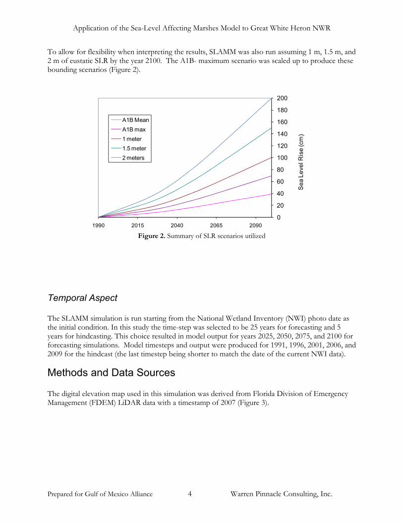
To allow for flexibility when interpreting the results, SLAMM was also run assuming 1 m, 1.5 m, and 2 m of eustatic SLR by the year 2100. The A1B- maximum scenario was scaled up to produce these bounding scenarios (Figure 2).
Figure 2. Summary of SLR scenarios utilized
0
20
40
60
80
100
120
140
160
180
200
1990 2015 2040 2065 2090
Sea
Lev
el R
ise
(cm
)
A1B MeanA1B max1 meter1.5 meter2 meters
Temporal Aspect The SLAMM simulation is run starting from the National Wetland Inventory (NWI) photo date as the initial condition. In this study the time-step was selected to be 25 years for forecasting and 5 years for hindcasting. This choice resulted in model output for years 2025, 2050, 2075, and 2100 for forecasting simulations. Model timesteps and output were produced for 1991, 1996, 2001, 2006, and 2009 for the hindcast (the last timestep being shorter to match the date of the current NWI data).
Methods and Data Sources The digital elevation map used in this simulation was derived from Florida Division of Emergency Management (FDEM) LiDAR data with a timestamp of 2007 (Figure 3).
Prepared for Gulf of Mexico Alliance 4 Warren Pinnacle Consulting, Inc.

Application of the Sea-Level Affecting Marshes Model to Great White Heron NWR
Figure 3: 2007 shade-relief elevation map of refuge and surrounding regions.
Two wetlands datasets were used in this simulation, one historical map for model hindcasting and the most current data used both for model projection and evaluation of model hindcast results. The wetlands layer used for hindcasting was produced by the NWI and was based on a 1986 photo date. While it might be preferable to have a longer hindcasting period (older NWI data) we were unable to obtain wetlands data produced prior to 1986. The wetland layer used for projection was also NWI-produced with a photo date of 2009 (Error! Reference source not found.).
Figure 4: SLAMM wetland classes from latest NWI dataset of 2009.
Prepared for Gulf of Mexico Alliance 5 Warren Pinnacle Consulting, Inc.

Application of the Sea-Level Affecting Marshes Model to Great White Heron NWR
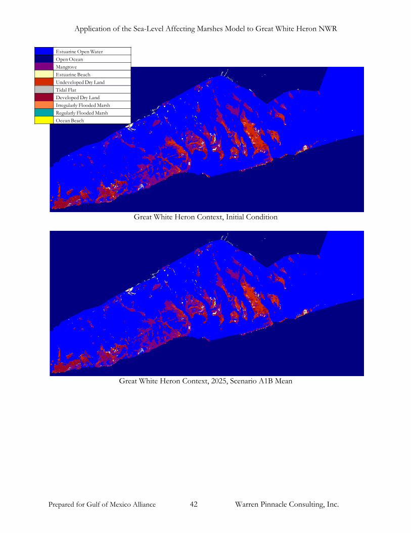
Converting the NWI survey into 10 m cells indicated that the approximately 207,600 acre refuge (approved acquisition boundary including water) is composed of the following categories:
Estuarine Open Water Estuarine Open Water 62.2% Open Ocean 32.7%
Mangrove Mangrove 4.3% Estuarine Beach Estuarine Beach 0.3% Undeveloped Dry Land Undeveloped Dry Land 0.3% Tidal Flat Tidal Flat 0.2% Developed Dry Land Developed Dry Land 0.1% Irregularly Flooded Marsh Irregularly Flooded Marsh <0.1% Regularly Flooded Marsh Regularly Flooded Marsh <0.1%
According to the National Wetland Inventory, there are no impounded or diked areas within Great White Heron NWR. The study area is located between two sites where historic sea-level rise trends have been measured: Key West to the west (2.24 mm/year) and Vaca Key to the east (2.78 mm/year). The global historic trend value was assigned an average of these two, 2.51 mm/year. The rate of sea level rise for this refuge has been slightly higher than the global average for the last 100 years (approximately 1.7 mm/year, IPCC 2007). Over 40 tide gauges were used to define the tide ranges for this site (Table 1 and Figure 5). The great diurnal tide range at this site varied from 0.31 m to 1.06 m. Tide data were spatially averaged over four “subsites” (Figure 8) as shown in the table below.
Prepared for Gulf of Mexico Alliance 6 Warren Pinnacle Consulting, Inc.

Application of the Sea-Level Affecting Marshes Model to Great White Heron NWR
Table 1: NOAA Gauges used for determining Tide Range and Salt Elevation
Station ID Site Name RelevantSubsite
Tide Range (GT in m)
Predicted Salt Elevation
8724463 Snipe Point, Snipe Keys, FL Global 0.864 0.575 8724397 Johnston Key, FL 2 0.604 0.402 8724373 Pumpkin Key, Sugarload Channel, FL Global 0.813 0.541 8724369 Sawyer Key (Inside), FL Global 0.744 0.495 8724307 Content Key, Ulf of Mexico, FL Global 1.059 0.704 8724246 Big Spanish Key, FL Global 0.980 0.652 8724209 Little Spanish Key Island, FL Global 0.878 0.584 8724172 Johnson Keys North, FL Global 0.670 0.446 8724139 Horeshoe Keys, FL 3 0.462 0.307 8724129 West Bahia Honda Key, FL 3 0.518 0.344 8724094 East Bahia Honda Key, FL 3 0.422 0.281 8724098 Cocoanut Key, FL 3 0.360 0.239 8724153 Johnson Keys South, FL 3 0.398 0.265 8724154 Little Pine Key South, FL 3 0.338 0.225 8724168 No Name Key, FL 3 0.345 0.229 8724196 Porpoise Key, FL 3 0.408 0.271 8724177 Little Pine Key North, FL 3 0.551 0.366 8724189 Water Key, Big Spanish Channel, FL 3 0.444 0.295 8724199 Crawl Key, Big Spanish Channel, FL 3 0.680 0.452 8724205 Mayo Key, FL 3 0.496 0.330 8724229 Annette Key, FL 3 0.734 0.488 8724231 Big Pine Key North End, FL 3 0.520 0.346 8724226 Big Pine Key Ne, FL 3 0.458 0.305 8724257 Howe Key Ne Point, FL Global 0.832 0.553 8724273 Water Keys South End, FL Global 0.781 0.519 8724264 Big Torch Key, West Side, FL 3 0.360 0.239 8724311 Racoon Key, FL Global 0.786 0.523 8724302 Knockemdown Key, FL Global 0.706 0.469 8724328 Cudjoe Key No. Point, FL Global 0.819 0.545 8724368 Sugarloaf Key (North End), FL Global 0.687 0.457 8724409 Inner Narrows, FL 2 0.664 0.442 8724427 Middle Narrows, FL 2 0.551 0.366 8724448 Waltz Key, FL 2 0.560 0.372 8724474 Duck Key Point, FL 2 0.626 0.416 8724485 Boca Chica, Ong Point, FL 2 0.516 0.343 8724507 Channel Key, FL 1 0.411 0.273 8724542 Sigsbee Park, Garrison Bight Channel, FL 1 0.454 0.302 8724571 Fleming Key, FL 1 0.443 0.295 8724441 Ohara Key, North Point, FL 2 0.554 0.368 8724347 Sugarloaf Key East Side, FL Global 0.554 0.368 8724227 Big Pine Key, West Side, FL 3 0.305 0.203 8724193 Bogie Channel Landing, Big Pine Key, FL 3 0.366 0.243
Prepared for Gulf of Mexico Alliance 7 Warren Pinnacle Consulting, Inc.
Application of the Sea-Level Affecting Marshes Model to Great White Heron NWR
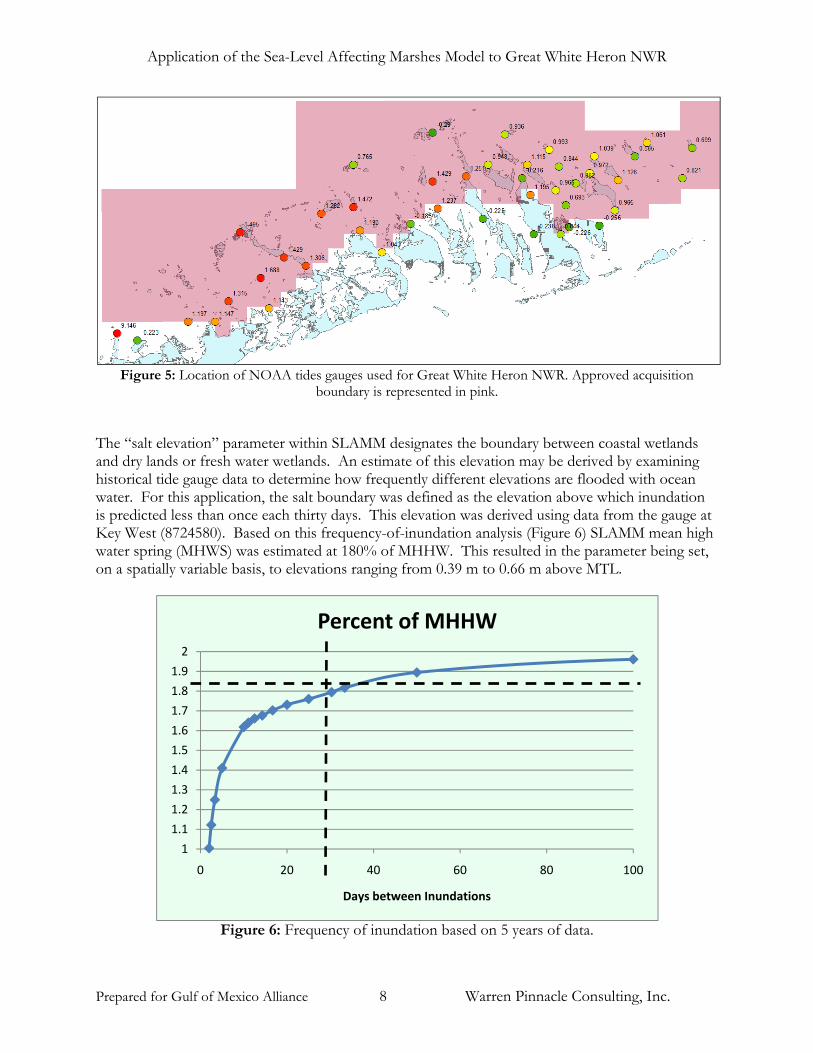
Figure 5: Location of NOAA tides gauges used for Great White Heron NWR. Approved acquisition
boundary is represented in pink. The “salt elevation” parameter within SLAMM designates the boundary between coastal wetlands and dry lands or fresh water wetlands. An estimate of this elevation may be derived by examining historical tide gauge data to determine how frequently different elevations are flooded with ocean water. For this application, the salt boundary was defined as the elevation above which inundation is predicted less than once each thirty days. This elevation was derived using data from the gauge at Key West (8724580). Based on this frequency-of-inundation analysis (Figure 6) SLAMM mean high water spring (MHWS) was estimated at 180% of MHHW. This resulted in the parameter being set, on a spatially variable basis, to elevations ranging from 0.39 m to 0.66 m above MTL.
Figure 6: Frequency of inundation based on 5 years of data.
1
1.1
1.2
1.3
1.4
1.5
1.6
1.7
1.8
1.9
2
0 20 40 60 80
Days between Inundations
Percent of MHHW
100
Prepared for Gulf of Mexico Alliance 8 Warren Pinnacle Consulting, Inc.

Application of the Sea-Level Affecting Marshes Model to Great White Heron NWR
Accretion rates for mangrove were lowered from the model default of 7.0 mm/year to 3.3 mm/year based on the results of a study performed using Cesium-137 dating in nearby Lignumvitae Key and Plantation Key (Callaway et al. 1997). The Callaway study makes a distinction between red mangrove, which grows along the lowest edges of the wetland, and black mangrove, which grows in the interior of mangrove swamps. Red mangroves are found to have higher average accretion rate than black mangrove. SLAMM does not make a distinction between black and red mangrove, so the average of red and black mangrove accretion rates was used to produce 3.3 mm/year. Beach sedimentation rates were increased from the SLAMM default of 0.5 mm/year to 1 mm/year and tidal flat erosion rates reduced from 0.5 mm/year to 0.1 mm/year. These changes were made to improve model results after initial hindcast calibrations predicted more beach loss than was observed. Predicted beach loss rates are highly uncertain as the available LiDAR data did not cover the vast majority of beach or tidal flat within the study area. For this reason, an estimation of beach and tidal flat elevations was created for both the hindcast and forecast. SLAMM elevation preprocessing produces a rough estimate of wetland elevations as a function of the tide range. For a more technical description of the elevation preprocessor, see the SLAMM 6 technical documentation (Clough et al. 2010). An analysis of wetland elevations using current LiDAR data indicated that the 5th percentile of elevation (in half-tide units ,or HTU) for mangrove is -0.63, as opposed to the model default minimum elevation of 0 (mean tide level). In other words, mangroves at this site were found to inhabit an elevation range below mean-tide level. Because this refuge is comprised mostly of mangrove habitats, the minimum elevation within the model was changed to -0.63 HTU. The MTL to NAVD88 correction was derived using NOAA’s VDATUM software. A raster of MTL to NAVD88 correction values was created for the study area using VDATUM software and applied to this simulation (Figure 7).
Figure 7: MTL-NAVD correction values (m).
Modeled U.S. Fish and Wildlife Service refuge boundaries for Florida are based on Approved Acquisition Boundaries as published on the FWS National Wildlife Refuge Data and Metadata
Prepared for Gulf of Mexico Alliance 9 Warren Pinnacle Consulting, Inc.

Application of the Sea-Level Affecting Marshes Model to Great White Heron NWR
website. The cell-size used for this analysis was 10 m by 10 m. Note that the SLAMM model will track partial conversion of cells based on elevation and slope. SUMMARY OF SLAMM INPUT PARAMETERS FOR GREAT WHITE HERON NWR
Parameter Global Subsite 1 Subsite 2 Subsite 3 Description Central Westernmost Western Eastern NWI Photo Date (YYYY) 2009 2009 2009 2009 DEM Date (YYYY) 2007 2007 2007 2007 Direction Offshore [n,s,e,w] North North North North Historic Trend (mm/yr) 2.51 2.24 2.24 2.78 MTL-NAVD88 (m) † † † † GT Great Diurnal Tide Range (m) 0.744 0.436 0.582 0.419 Salt Elev. (m above MTL) 0.66 0.39 0.52 0.37 Marsh Erosion (horz. m /yr) 1.8 1.8 1.8 1.8 Swamp Erosion (horz. m /yr) 1 1 1 1 T.Flat Erosion (horz. m /yr) 0.1 0.1 0.1 0.1 Reg. Flood Marsh Accr (mm/yr) 3.9 3.9 3.9 3.9 Irreg. Flood Marsh Accr (mm/yr) 4.7 4.7 4.7 4.7 Tidal Fresh Marsh Accr (mm/yr) 5.9 5.9 5.9 5.9 Beach Sed. Rate (mm/yr) 1 1 1 1 Freq. Overwash (years) 4 4 4 4
Use Elev Pre-processor [True,False]
Beach & T.Flat only
Beach & T.Flat only
Beach & T.Flat only
Beach & T.Flatonly
† Spatially variable raster map used in place of fixed values.
Prepared for Gulf of Mexico Alliance 10 Warren Pinnacle Consulting, Inc.

Application of the Sea-Level Affecting Marshes Model to Great White Heron NWR
Figure 8: Input subsites for model application.
Subsite 2
Subsite 1
Subsite 3
Prepared for Gulf of Mexico Alliance 11 Warren Pinnacle Consulting, Inc.

Application of the Sea-Level Affecting Marshes Model to Great White Heron NWR
Results The analysis of Great White Heron NWR included a “hindcasting” analysis. Hindcasting is performed by starting a simulation at the photo date of the oldest-available wetlands data, running it through the present day, and comparing the output to present-day NWI data. The primary goals of hindcasting are to assess the predictive capacity of a model and potentially to improve model predictions through calibration. In the case of SLAMM, hindcasting is used to determine whether or not the model is correctly predicting the effect of the observed sea level signal on the wetland types in a given study area. As with all environmental models, uncertainty within input data and model processes limit model precision. Some error within hindcast results are likely caused by the relative simplicity of the SLAMM model. Additionally, the NWI data may introduce error due to lack of horizontal precision or misclassified land coverage, while the DEM may introduce error due to limitations in LiDAR accuracy. Additional error is encountered when the DEM data and NWI data were collected during different time-periods (not temporally synoptic). Lack of precise tidal data or other spatial coverages may further reduce model accuracy. Although historical DEM data is usually not used (since older technology generally produced low-vertical-resolution data) SLAMM has two methods to compensate for a lack of historical DEM data. The first method is by utilizing the elevation pre-processor, which estimates elevation ranges as a function of tide ranges and estimated relationships between wetland types and tide ranges (Clough et al. 2010). As an alternative to using the pre-processor, the second method involves a modification of present-day, high-resolution DEM so that it reflects the historical land-cover date by reversing the estimated land uplift or subsidence which took place in the years between the NWI and DEM dates. This process ignores changes due to erosion, accretion, or sedimentation, however. Because the historical data is relatively recent, the second approach was used in analysis of Great White Heron NWR. There are two sources of error in these hindcasting analyses, the first being the minor differences predicted by SLAMM even without a SLR signal. A simulation with no SLR signal is referred to as a “time-zero” simulation in which SLAMM tries to predict the current condition. Due to local factors, DEM and NWI uncertainty, and simplifications within the SLAMM conceptual model, some cells inevitably fall below their lowest allowable elevation category and are immediately converted. These cells represent outliers on the distribution of elevations for a given land-cover type. Generally, a threshold tolerance of up to 5% change is allowed for in major land cover categories in our analyses. The second source of error would be errors in SLAMM predictions given a SLR signal. This second source of error is generally more interesting and important. We need to determine if SLAMM can accurately predict growth or loss trends for major land-cover categories. For this reason, we assess SLAMM hindcast accuracy on results after the “time-zero” model adjustment has taken place. There are several metrics that may be employed to judge the accuracy of the model based on the hindcast results. One possibility would be to see whether SLAMM can predict a given cell’s wetland type correctly. Because of the high potential for local uncertainty the method used for evaluation focuses on assessing the capability of the model to predict overall trends in land-cover over time. Additionally, assessing model accuracy on a cell-by-cell basis is a metric that has been shown to be sensitive to the cell size utilized (Chen & Pontius 2010). Prepared for Gulf of Mexico Alliance 12 Warren Pinnacle Consulting, Inc.

Application of the Sea-Level Affecting Marshes Model to Great White Heron NWR
The primary metric used to evaluate SLAMM hindcast results in this study is the percent of the land cover lost during the model simulation for the primary wetland/vegetation types. The percentage loss predicted by the model is compared to the percentage of the actual land cover lost determined by comparing the historical and contemporary NWI datasets. In addition, if there are significant spatial trends visible when comparing historical data to present-day data (e.g. the majority of marsh lost occurs in the upper-right quadrant) maps of hindcasting predictions are qualitatively assessed to ensure that these trends are also captured within the model results itself.
Hindcast Results Based on historical records, during the period between 1986 and 2009, approximately 6 cm of eustatic SLR occurred. Based on this sea-level rise signal, SLAMM predicts minor losses for about half of the land categories between 1986 and 2009. Predicted losses of estuarine beach and tidal flat were most extreme, likely due to uncertainty over initial-condition elevations for these classes (which were omitted from the LiDAR coverage for the most part).
Table 2: Hindcast results
Land Category
Study area observed in 2009 (acres)
Study area predicted by hindcast (acres)
Observed loss 1986-2009 (acres) (1)
Predicted loss 1986-2009 (acres) (1)
Estuarine Open Water 129133 129871 0 (0.0%) -213 (-0.2%)
Open Ocean 67808 67808 0 (0.0%) 0 (0.0%)
Mangrove 8850 8315 0 (0.0%) 68 (0.8%)
Estuarine Beach 592 540 0 (0.0%) 46 (7.9%)
Undeveloped Dry Land 523 402 6 (1.2%) 30 (6.9%)
Tidal Flat 452 459 0 (0.0%) 63 (12.1%)
Developed Dry Land 209 182 1 (0.2%) 6 (3.2%)
Irregularly Flooded Marsh 65 60 0 (0.0%) 0 (0.0%)
Regularly Flooded Marsh 6 6 0 (0.0%) 0 (0.0%) (1) In parenthesis percentage loss with respect of the initial land cover category considered. A negative sign indicates a gain. While the predicted study area is quite similar to the observed study area in terms of overall percentages, the percentage of land cover lost during the hindcast is somewhat greater than the percentage changes observed in the NWI data for some land cover types present in the study area. For example, beach-loss rates are predicted at 7.9% and tidal flat at 12.1%, compared with an actual loss for both land types of zero percent. More dry-land loss is predicted that observed and this may be due to uncertainty in the height at which salt elevation converts dry land to wetland or due to uncertainty in LiDAR data. Given the similarity of predicted and observed maps of dry land (red regions below) we did not pursue calibrating the model further to reduce dry-land loss rates.
Prepared for Gulf of Mexico Alliance 13 Warren Pinnacle Consulting, Inc.

Application of the Sea-Level Affecting Marshes Model to Great White Heron NWR
Great White Heron NWR, 2009, 0.54 m scenario (hindcast result)
Great White Heron NWR, (2009 NWI data)
In general, SLAMM model predictions and observed historical changes are both minimal. Looking at a map of the study area and comparing that with SLAMM simulations, few differences are obvious. Overall, the lack of appreciable difference in the historical and present-day datasets led to a less robust hindcast analysis than would have been achieved if more land-cover changes were observed (given a more significant SLR signal).
Estuarine Open WaterEstuarine Open WaterOpen Ocean
MangroveMangrove
Estuarine BeachEstuarine BeachUndeveloped Dry Land
Tidal Fla tTidal Flat
Developed Dry LandDeveloped Dry Land
Irregularly Flooded MarshIrregularly Flooded Marsh
R egularly Flooded MarshRegularly Flooded Marsh
Ocean BeachOcean Beach
Undeveloped Dry Land
Prepared for Gulf of Mexico Alliance 14 Warren Pinnacle Consulting, Inc.

Application of the Sea-Level Affecting Marshes Model to Great White Heron NWR
GWH Raster Hindcast 0.54 Meters Results in Acres
Initial Time-zero 2009
Estuarine Open Water Estuarine Open Water 129133.1 129658.6 129871.4Open Ocean 67807.6 67807.6 67807.6
Mangrove Mangrove 8849.5 8383.1 8314.8
Estuarine Beach Estuarine Beach 591.9 586.3 540.2
Undeveloped Dry Land Undeveloped Dry Land 529.2 432.0 402.4
Tidal Flat Tidal Flat 451.8 522.3 459.3
Developed Dry Land Developed Dry Land 209.0 187.9 181.9
Irregularly Flooded Marsh Irregularly Flooded Marsh 65.0 59.9 59.9
Regularly Flooded Marsh Regularly Flooded Marsh 6.3 5.5 5.5
Ocean Beach Ocean Beach 0.0 0.1 0.2
Total (incl. water) 207643.3 207643.3 207643.3
Prepared for Gulf of Mexico Alliance 15 Warren Pinnacle Consulting, Inc.

Application of the Sea-Level Affecting Marshes Model to Great White Heron NWR
Great White Heron NWR, hindcast time zero
Estuarine Open WaterEstuarine Open WaterOpen Ocean
MangroveMangrove
Estuarine BeachEstuarine BeachUndeveloped Dry Land
Tidal Fla tTidal Flat
Developed Dry LandDeveloped Dry Land
Irregularly Flooded MarshIrregularly Flooded Marsh
R egularly Flooded MarshRegularly Flooded Marsh
Ocean BeachOcean Beach
Undeveloped Dry Land
Great White Heron NWR, 2009, hindcast prediction
Prepared for Gulf of Mexico Alliance 16 Warren Pinnacle Consulting, Inc.

Application of the Sea-Level Affecting Marshes Model to Great White Heron NWR
Forecast SLAMM predicts that Great White Heron NWR will be severely impacted by sea level rise. The majority of refuge mangrove is predicted to be lost in scenarios above 0.69 m. More than 50% of refuge dry land is predicted to be lost across all SLR scenarios.
SLR by 2100 (m) 0.39 0.69 1 1.5 2 Mangrove 10% 37% 77% 95% 96% Estuarine Beach 58% 92% 98% 100% 100% Undeveloped Dry Land 56% 83% 95% 98% 98% Tidal Flat 82% 85% 88% 86% 83% Developed Dry Land 51% 84% 95% 98% 99% Irregularly Flooded Marsh 12% 74% 94% 95% 95% Regularly Flooded Marsh 40% 68% 69% 69% 69%
Predicted Loss Rates of Land Categories by 2100 Given Simulated
Scenarios of Eustatic Sea Level Rise
GWH Forecast Raster IPCC Scenario A1B-Mean, 0.39 M SLR Eustatic by 2100 Results in Acres
Initial 2025 2050 2075 2100 Estuarine Open Water
Estuarine Open Water 129133.1 129786.0 130202.9 130717.4 131117.6
Open Ocean Open Ocean 67807.6 67807.6 67807.6 67807.6 67807.7
Mangrove Mangrove 8849.5 8269.2 8255.7 8143.1 7985.9
Estuarine Beach Estuarine Beach 591.9 564.6 479.0 363.8 249.6
Undeveloped Dry Land
Undeveloped Dry Land 523.0 401.0 349.2 291.7 228.6
Tidal Flat Tidal Flat 451.8 561.9 311.9 111.2 83.4
Developed Dry Land
Developed Dry Land 208.5 182.6 166.8 138.7 103.0Irregularly Flooded Marsh
Irregularly Flooded Marsh 65.0 58.3 58.3 58.3 56.9Regularly Flooded Marsh
Regularly Flooded Marsh 6.3 5.1 5.0 4.3 3.8
Ocean Beach Ocean Beach 0.0 0.2 0.3 0.4 0.4
Total (incl. water) 207636.7 207636.7 207636.7 207636.7 207636.7
Prepared for Gulf of Mexico Alliance 17 Warren Pinnacle Consulting, Inc.

Application of the Sea-Level Affecting Marshes Model to Great White Heron NWR
Great White Heron NWR, Initial Condition, 2009
Estuarine Open WaterEstuarine Open WaterOpen Ocean
MangroveMangrove
Estuarine BeachEstuarine BeachUndeveloped Dry Land
Tidal Fla tTidal Flat
Developed Dry LandDeveloped Dry Land
Irregularly Flooded MarshIrregularly Flooded Marsh
R egularly Flooded MarshRegularly Flooded Marsh
Ocean BeachOcean Beach
Undeveloped Dry Land
Great White Heron NWR, 2025, Scenario A1B Mean
Prepared for Gulf of Mexico Alliance 18 Warren Pinnacle Consulting, Inc.
Application of the Sea-Level Affecting Marshes Model to Great White Heron NWR
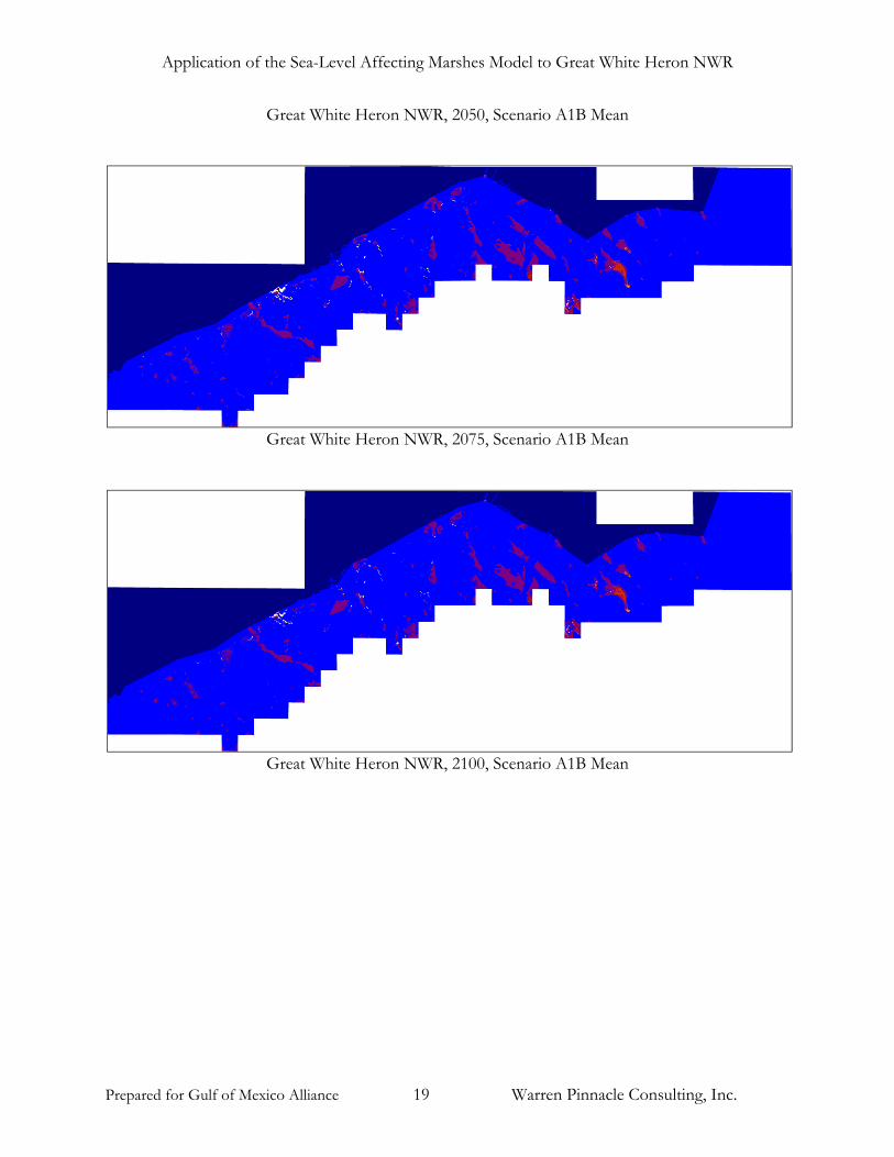
Great White Heron NWR, 2050, Scenario A1B Mean
Great White Heron NWR, 2075, Scenario A1B Mean
Great White Heron NWR, 2100, Scenario A1B Mean
Prepared for Gulf of Mexico Alliance 19 Warren Pinnacle Consulting, Inc.

Application of the Sea-Level Affecting Marshes Model to Great White Heron NWR
GWH Forecast Raster IPCC Scenario A1B-Max, 0.69 m SLR Eustatic by 2100 Results in Acres
Initial 2025 2050 2075 2100Estuarine Open Water
Estuarine Open Water 129133.1 129927.1 130827.1 132102.9 133965.7
Open Ocean Open Ocean 67807.6 67807.6 67807.6 67807.7 67807.9
Mangrove Mangrove 8849.5 8223.0 7945.0 7131.0 5604.0
Estuarine Beach Estuarine Beach 591.9 542.7 384.6 168.0 48.3
Undeveloped Dry Land
Undeveloped Dry Land 523.0 389.9 313.0 206.6 90.7
Tidal Flat Tidal Flat 451.8 502.8 152.7 89.0 66.9
Developed Dry Land
Developed Dry Land 208.5 180.1 150.0 91.1 33.9Irregularly Flooded Marsh
Irregularly Flooded Marsh 65.0 58.2 52.5 37.8 16.9Regularly Flooded Marsh
Regularly Flooded Marsh 6.3 4.9 3.7 2.3 2.0
Ocean Beach Ocean Beach 0.0 0.2 0.4 0.3 0.2
Total (incl. water) 207636.7 207636.7 207636.7 207636.7 207636.7
Prepared for Gulf of Mexico Alliance 20 Warren Pinnacle Consulting, Inc.

Application of the Sea-Level Affecting Marshes Model to Great White Heron NWR
Great White Heron NWR, Initial Condition, 2009
Estuarine Open WaterEstuarine Open WaterOpen Ocean
MangroveMangrove
Estuarine BeachEstuarine BeachUndeveloped Dry Land
Tidal Fla tTidal Flat
Developed Dry LandDeveloped Dry Land
Irregularly Flooded MarshIrregularly Flooded Marsh
R egularly Flooded MarshRegularly Flooded Marsh
Ocean BeachOcean Beach
Undeveloped Dry Land
Great White Heron NWR, 2025, Scenario A1B Maximum
Great White Heron NWR, 2050, Scenario A1B Maximum
Prepared for Gulf of Mexico Alliance 21 Warren Pinnacle Consulting, Inc.

Application of the Sea-Level Affecting Marshes Model to Great White Heron NWR
Great White Heron NWR, 2075, Scenario A1B Maximum
Great White Heron NWR, 2100, Scenario A1B Maximum
Prepared for Gulf of Mexico Alliance 22 Warren Pinnacle Consulting, Inc.

Application of the Sea-Level Affecting Marshes Model to Great White Heron NWR
GWH Forecast Raster 1 m Eustatic SLR by 2100 Results in Acres
Initial 2025 2050 2075 2100Estuarine Open Water
Estuarine Open Water 129133.1 130108.2 131563.2 134438.7 137692.1
Open Ocean Open Ocean 67807.6 67807.6 67807.6 67807.8 67808.0
Mangrove Mangrove 8849.5 8153.1 7417.4 5103.5 2025.6
Estuarine Beach Estuarine Beach 591.9 517.8 281.1 51.7 11.9
Undeveloped Dry Land
Undeveloped Dry Land 523.0 377.8 271.3 111.8 26.7
Tidal Flat Tidal Flat 451.8 434.4 125.1 67.8 55.6
Developed Dry Land
Developed Dry Land 208.5 177.0 127.5 43.7 10.8Irregularly Flooded Marsh
Irregularly Flooded Marsh 65.0 56.0 40.5 9.4 4.0Regularly Flooded Marsh
Regularly Flooded Marsh 6.3 4.5 2.5 2.0 2.0
Ocean Beach Ocean Beach 0.0 0.2 0.4 0.2 0.0
Total (incl. water) 207636.7 207636.7 207636.7 207636.7 207636.7
Prepared for Gulf of Mexico Alliance 23 Warren Pinnacle Consulting, Inc.

Application of the Sea-Level Affecting Marshes Model to Great White Heron NWR
Great White Heron NWR, Initial Condition, 2009
Estuarine Open WaterEstuarine Open WaterOpen Ocean
MangroveMangrove
Estuarine BeachEstuarine BeachUndeveloped Dry Land
Tidal Fla tTidal Flat
Developed Dry LandDeveloped Dry Land
Irregularly Flooded MarshIrregularly Flooded Marsh
R egularly Flooded MarshRegularly Flooded Marsh
Ocean BeachOcean Beach
Undeveloped Dry Land
Great White Heron NWR, 2025, 1 m
Great White Heron NWR, 2050, 1 m
Prepared for Gulf of Mexico Alliance 24 Warren Pinnacle Consulting, Inc.

Application of the Sea-Level Affecting Marshes Model to Great White Heron NWR
Great White Heron NWR, 2075, 1 m
Great White Heron NWR, 2100, 1 m
Prepared for Gulf of Mexico Alliance 25 Warren Pinnacle Consulting, Inc.

Application of the Sea-Level Affecting Marshes Model to Great White Heron NWR
GWH Forecast Raster 1.5 m Eustatic SLR by 2100 Results in Acres
Initial 2025 2050 2075 2100Estuarine Open Water
Estuarine Open Water 129133.1 130431.1 133324.8 138085.1 139273.4
Open Ocean Open Ocean 67807.6 67807.6 67807.7 67808.0 67808.0
Mangrove Mangrove 8849.5 8011.3 6004.8 1629.7 469.0
Estuarine Beach Estuarine Beach 591.9 475.1 109.9 12.0 1.3
Undeveloped Dry Land
Undeveloped Dry Land 523.0 359.6 195.3 31.6 10.9
Tidal Flat Tidal Flat 451.8 324.5 92.6 52.7 64.3
Developed Dry Land
Developed Dry Land 208.5 170.8 85.0 11.8 4.2Irregularly Flooded Marsh
Irregularly Flooded Marsh 65.0 52.3 14.1 3.7 3.5Regularly Flooded Marsh
Regularly Flooded Marsh 6.3 4.0 2.1 2.0 2.0
Ocean Beach Ocean Beach 0.0 0.3 0.3 0.0 0.0
Total (incl. water) 207636.7 207636.7 207636.7 207636.7 207636.7
Prepared for Gulf of Mexico Alliance 26 Warren Pinnacle Consulting, Inc.

Application of the Sea-Level Affecting Marshes Model to Great White Heron NWR
Great White Heron NWR, Initial Condition, 2009
Estuarine Open WaterEstuarine Open WaterOpen Ocean
MangroveMangrove
Estuarine BeachEstuarine BeachUndeveloped Dry Land
Tidal Fla tTidal Flat
Developed Dry LandDeveloped Dry Land
Irregularly Flooded MarshIrregularly Flooded Marsh
R egularly Flooded MarshRegularly Flooded Marsh
Ocean BeachOcean Beach
Undeveloped Dry Land
Great White Heron NWR, 2025, 1.5 m
Great White Heron NWR, 2050, 1.5 m
Prepared for Gulf of Mexico Alliance 27 Warren Pinnacle Consulting, Inc.

Application of the Sea-Level Affecting Marshes Model to Great White Heron NWR
Great White Heron NWR, 2075, 1.5 m
Great White Heron NWR, 2100, 1.5 m
Prepared for Gulf of Mexico Alliance 28 Warren Pinnacle Consulting, Inc.

Application of the Sea-Level Affecting Marshes Model to Great White Heron NWR
GWH Forecast Raster 2 Meters Eustatic SLR by 2100 Results in Acres
Initial 2025 2050 2075 2100Estuarine Open Water
Estuarine Open Water 129133.1 130795.6 135655.7 139100.3 139418.6
Open Ocean Open Ocean 67807.6 67807.6 67807.8 67808.0 67808.0
Mangrove Mangrove 8849.5 7829.7 3884.2 645.2 315.0
Estuarine Beach Estuarine Beach 591.9 430.3 48.4 1.4 1.8
Undeveloped Dry Land
Undeveloped Dry Land 523.0 342.3 114.8 11.4 10.3
Tidal Flat Tidal Flat 451.8 215.5 73.4 59.1 75.6
Developed Dry Land
Developed Dry Land 208.5 163.9 45.0 5.8 1.9Irregularly Flooded Marsh
Irregularly Flooded Marsh 65.0 47.9 5.1 3.5 3.5Regularly Flooded Marsh
Regularly Flooded Marsh 6.3 3.5 2.0 2.0 2.0
Ocean Beach Ocean Beach 0.0 0.3 0.2 0.0 0.0
Total (incl. water) 207636.7 207636.7 207636.7 207636.7 207636.7
Prepared for Gulf of Mexico Alliance 29 Warren Pinnacle Consulting, Inc.

Application of the Sea-Level Affecting Marshes Model to Great White Heron NWR
Great White Heron NWR, Initial Condition, 2009
Estuarine Open WaterEstuarine Open WaterOpen Ocean
MangroveMangrove
Estuarine BeachEstuarine BeachUndeveloped Dry Land
Tidal Fla tTidal Flat
Developed Dry LandDeveloped Dry Land
Irregularly Flooded MarshIrregularly Flooded Marsh
R egularly Flooded MarshRegularly Flooded Marsh
Ocean BeachOcean Beach
Undeveloped Dry Land
Great White Heron NWR, 2025, 2 m
Great White Heron NWR, 2050, 2 m
Prepared for Gulf of Mexico Alliance 30 Warren Pinnacle Consulting, Inc.

Application of the Sea-Level Affecting Marshes Model to Great White Heron NWR
Great White Heron NWR, 2075, 2 m
Great White Heron NWR, 2100, 2 m
Prepared for Gulf of Mexico Alliance 31 Warren Pinnacle Consulting, Inc.

Application of the Sea-Level Affecting Marshes Model to Great White Heron NWR
Erosion Maps Horizontal erosion of mangroves was predicted to be high (>10 m) in many locations of the refuge, as the following map illustrates (Figure 9). Not surprisingly, erosion is most extreme along low-lying coastal regions.
Figure 9: Horizontal marsh erosion (m).
Prepared for Gulf of Mexico Alliance 32 Warren Pinnacle Consulting, Inc.

Application of the Sea-Level Affecting Marshes Model to Great White Heron NWR
Elevation Uncertainty Analysis An elevation uncertainty analysis was performed for this model application in order to estimate the impact of terrain uncertainty on SLAMM outputs. This analysis took into account both the uncertainty related to the elevation data as well as the VDatum correction values. According to the vertical accuracy report associated with these data (Conner 2008), the root mean squared error (RMSE) for these LiDAR data are as follows
Land Type RMSE (ft) RMSE (m) Bare‐earth and low grass 0.19 0.058 Brush lands and low trees 0.27 0.082
Forested Area 0.13 0.040 Urban Areas 0.15 0.046
All Data Combined 0.17 0.052 In order to be conservative and to assess the full potential effects of elevation data uncertainty on these model predictions, we used the RMSE from the land-cover class that had the highest associated error “brush lands and low trees”. According the VDatum website the RMSE for the study region is 0.041 m (NOAA 2010). This value was determined by combining the uncertainty associated with the NAVD to MSL transformation (0.03 m) and MSL to MTL transformation (0.011 m). The means of evaluating elevation data uncertainty was the application of a spatially autocorrelated error field to the existing digital elevation map in the manner of Heuvelink . In this application, an error field for both the DEM uncertainty and the VDatum correction uncertainty were applied to the existing DEM. This approach uses the normal distribution as specified by the Root Mean Squared Error for the dataset and applies it randomly over the entire study area, but with spatial autocorrelation included (Figure 10). Since elevation error is generally spatially autocorrelated (Hunter and Goodchild 1997), this method provides a means to calculate a number of equally-likely elevation maps given error statistics about the data set. A stochastic analysis may then be run (running the model with each of these elevation maps) to assess the overall effects of elevation uncertainty. Heuvelink’s method has been widely recommended as an approach for assessing the effects of elevation data uncertainty (Hunter and Goodchild 1997) (Darnell et al. 2008). In this analysis, it was assumed that elevation errors were strongly spatially autocorrelated, using a “p-value” of 0.24991.
1 A p-value of zero is no spatial autocorrelation and 0.25 is perfect correlation (i.e. not possible). P-values must be less than 0.25.
Prepared for Gulf of Mexico Alliance 33 Warren Pinnacle Consulting, Inc.

Application of the Sea-Level Affecting Marshes Model to Great White Heron NWR
Figure 10: A spatially autocorrelated error field using parameters
from this model application(m). For the uncertainty analysis, 50 iterations were run for the study area representing approximately 100 hours of CPU time. The model was run with 0.69 m of eustatic SLR by 2100 in each iteration. In terms of overall acreage change, the effects of elevation uncertainty within this modeling analysis were quite limited, with the coefficient of variance (CV) remaining below 2% for refuge mangrove, which constitutes the vast majority of the refuge. These results reveal that mangrove (Figure 12) varies little with variable elevation values and, more generally, that the model is not sensitive to errors on this scale. However, for the remaining land categories the effects of elevation uncertainty were quite significant.
Table 3. Results of Elevation Uncertainty Analysis (in acres). Variable Name Min Max Deterministic St Dev CV
Mangrove 5359.6 5746.3 5604.0 84.2 1.50%
Undeveloped Dry Land 68.6 106.2 90.7 9.4 10.70%
Developed Dry Land 25.0 47.9 33.9 4.6 13.50%
Irreg. Flooded Marsh 11.4 28.1 16.9 4.1 21.10%
Regularly Flooded Marsh 2.0 2.7 2.0 0.1 6.40%
Ocean Beach 0.0 0.3 0.2 0.1 40.40%
These model results suggest that methods that uniformly apply the 95th percentile uncertainty associated with the LiDAR data across an entire surface may be overly conservative (Gesch 2009).
Prepared for Gulf of Mexico Alliance 34 Warren Pinnacle Consulting, Inc.

Application of the Sea-Level Affecting Marshes Model to Great White Heron NWR
Figure 11: The frequency of acres by 2100 for undeveloped dry land by 2100
The initial condition for undeveloped dry land was 523 acres. Given elevation uncertainty, these results suggest a loss ranging from 80% to 87% by 2100.
Prepared for Gulf of Mexico Alliance 35 Warren Pinnacle Consulting, Inc.

Application of the Sea-Level Affecting Marshes Model to Great White Heron NWR
Figure 12: The frequency of acres by 2100 for mangrove by 2100.
The initial condition for mangrove was 8849 acres. Given elevation uncertainty, these results suggest a loss ranging from 35 to 39% by 2100. Prepared for Gulf of Mexico Alliance 36 Warren Pinnacle Consulting, Inc.

Application of the Sea-Level Affecting Marshes Model to Great White Heron NWR
The variability in predicted losses due to elevation uncertainty is summarized in Table 4. Generally the range in predicted losses is relatively narrow compared with other sources of model uncertainty (e.g. different SLR scenarios).
Table 4. Predicted Range of Losses Due to Elevation Data Uncertainty
Variable Name Predicted loss
(%) Min Loss
(%) Max Loss
(%)
Mangrove 37 35 39
Undeveloped Dry Land 83 80 87
Developed Dry Land 84 77 88
Irreg. Flooded Marsh 74 57 82
Regularly Flooded Marsh 68 57 68
Prepared for Gulf of Mexico Alliance 37 Warren Pinnacle Consulting, Inc.

Application of the Sea-Level Affecting Marshes Model to Great White Heron NWR
Discussion In the SLAMM forecast of Great White Heron National Wildlife Refuge, inundation effects are severe for nearly every land category in the refuge across the SLR-scenario spectrum. Islands with relatively high land elevations, such as Little Pine Key and Howe Key, are most resilient. Many of the keys west of the Snipe Keys, including the Lower Harbor Keys and Mud Keys, fare poorly even in the moderate SLR scenarios primarily due to their relatively-low initial-condition elevations. Mangrove loss is relatively minimal in the lowest SLR scenario (0.39 m of eustatic SLR by 2100) because of mangrove accretion and mangrove expansion onto previously dry lands. Mangrove intrusion onto dry land is particularly prevalent on Little Pine Key and Porpoise Key, as well as the eastern shoreline of Raccoon Key. In higher SLR scenarios, mangrove accretion fails to keep up with sea-level rise and mangrove populations decline dramatically. SLAMM generally uses a mangrove accretion value of 7 mm/year, but this parameter was modified for this site based on local data suggesting mangrove accretion values of 4 mm/year for red mangrove and 2.7 mm/year for black mangrove. Because SLAMM averages red and black mangrove accretion rates, some additional model uncertainty is introduced. More in general, lack of mangrove accretion feedbacks, as well as a lack of spatially variable mangrove accretion rates, introduces additional uncertainty into the modeling of a refuge composed primarily of mangroves. As the overwhelming majority of tidal flat and estuarine beach lacked elevation data, the elevations of these types of land cover were estimated. This introduces significant uncertainty into model results for these categories as model elevation assumptions may not reflect current elevations for these land types.
Prepared for Gulf of Mexico Alliance 38 Warren Pinnacle Consulting, Inc.

Application of the Sea-Level Affecting Marshes Model to Great White Heron NWR
References
Callaway, J. C., DeLaune, R. D., and Jr., W. H. P. (1997). “Sediment Accretion Rates from Four Coastal Wetlands along the Gulf of Mexico.” Journal of Coastal Research, 13(1), 181-191.
Chen, H., and Pontius, R. G. (2010). “Sensitivity of a Land Change Model to Pixel Resolution and Precision of the Independent Variable.” Environmental Modeling & Assessment.
Chen, J. L., Wilson, C. R., and Tapley, B. D. (2006). “Satellite Gravity Measurements Confirm Accelerated Melting of Greenland Ice Sheet.” Science, 1129007.
Clark, P. U. (2009). Abrupt Climate Change: Final Report, Synthesis and Assessment Product 3. 4. DIANE Publishing.
Clough, J. S., Park, R., and Fuller, R. (2010). “SLAMM 6 beta Technical Documentation.” Available at http://warrenpinnacle.com/prof/SLAMM.
Conner, J. (2008). “Vertical Accuracy Report.” 3001, Inc., CH2M Hill, Inc.
Council for Regulatory Environmental Modeling. (2008). Draft guidance on the development, evaluation, and application of regulatory environmental models. Draft, Washington, DC.
Craft, C., Clough, J., Ehman, J., Joye, S., Park, R., Pennings, S., Guo, H., and Machmuller, M. (2009). “Forecasting the effects of accelerated sea-level rise on tidal marsh ecosystem services.” Frontiers in Ecology and the Environment, 7(2), 73-78.
Darnell, A. R., Tate, N. J., and Brunsdon, C. (2008). “Improving user assessment of error implications in digital elevation models.” Computers, Environment and Urban Systems, 32(4), 268-277.
Galbraith, H., Jones, R., Park, R., Clough, J., Herrod-Julius, S., Harrington, B., and Page, G. (2002). “Global Climate Change and Sea Level Rise: Potential Losses of Intertidal Habitat for Shorebirds.” Waterbirds, 25(2), 173.
Gesch, D. B. (2009). “Analysis of Lidar Elevaiton Data for Improved Identification and Delineation of Lands Vulnerable to Sea-Level Rise.” Jounral of Coastal Research, (53), 49-58.
Glick, P., Clough, J., and Nunley, B. (2007). Sea-level Rise and Coastal Habitats in the Pacific Northwest An Analysis for Puget Sound, Southwestern Washington, and Northwestern Oregon. National Wildlife Federation.
Grinsted, A., Moore, J. C., and Jevrejeva, S. (2009). “Reconstructing sea level from paleo and projected temperatures 200 to 2100 ad.” Climate Dynamics, 34(4), 461-472.
Heuvelink, G. B. M. (1998). Error propagation in environmental Modeling with GIS. Taylor & Francis.
Hunter, G. J., and Goodchild, M. F. (1997). “Modeling the uncertainty of slope and aspect estimates derived from spatial databases.” Geographical Analysis, 29(1), 35–49.
IPCC. (2001). Climate Change 2001: The Scientific Basis. Contribution of Working Group I to the Third Assessment Report of the Intergovernmental Panel on Climate Change. Cambridge University Press, Cambrdige, United Kingdom, 881.
IPCC. (2007). Climate change 2007 : the physical science basis. Cambridge university press, Cambridge.
Lee, J. K., Park, R. A., and Mausel, P. W. (1992). Application of geoprocessing and simulation modeling to estimate impacts of sea level rise on the northeast coast of Florida.
Prepared for Gulf of Mexico Alliance 39 Warren Pinnacle Consulting, Inc.

Application of the Sea-Level Affecting Marshes Model to Great White Heron NWR
Monaghan, A. J., Bromwich, D. H., Fogt, R. L., Wang, S., Mayewski, P. A., Dixon, D. A., Ekaykin, A., Frezzotti, M., Goodwin, I., Isaksson, E., Kaspari, S. D., Morgan, V. I., Oerter, H., Van Ommen, T. D., Van der Veen, C. J., and Wen, J. (2006). “Insignificant Change in Antarctic Snowfall Since the International Geophysical Year.” Science, 313(5788), 827-831.
Moorhead, K. K., and Brinson, M. M. (1995). “Response of Wetlands to Rising Sea Level in the Lower Coastal Plain of North Carolina.” Ecological Applications, 5(1), 261-271.
National Wildlife Federation, and Florida Wildlife Federation. (2006). An Unfavorable Tide: Global Warming, Coastal Habitats and Sportfishing in Florida.
NOAA. (2010). “Estimation of Vertical Uncertainties in VDatum.”
Park, R. A., Trehan, M., Mausel, P. W., and Howe, R.C. (1989). “The Effects of Sea Level Rise on U.S. Coastal Wetlands.” The Potential Effects of Global Climate Change on the United States: Appendix B - Sea Level Rise, U.S. Environmental Protection Agency, Washington, DC, 1-1 to 1-55.
Park, R. A., Lee, J. K., Mausel, P. W., and Howe, R. C. (1991). “Using remote sensing for modeling the impacts of sea level rise..” World Resources Review, 3, 184-220.
Park, R. A., Lee, J. K., and Canning, D. J. (1993). “Potential Effects of Sea-Level Rise on Puget Sound Wetlands.” Geocarto International, 8(4), 99.
Pfeffer, W. T., Harper, J. T., and O'Neel, S. (2008). “Kinematic Constraints on Glacier Contributions to 21st-Century Sea-Level Rise.” Science, 321(5894), 1340-1343.
Rahmstorf, S. (2007). “A Semi-Empirical Approach to Projecting Future Sea-Level Rise.” Science, 315(5810), 368-370.
Titus, J. G., Park, R. A., Leatherman, S. P., Weggel, J. R., Greene, M. S., Mausel, P. W., Brown, S., Gaunt, C., Trehan, M., and Yohe, G. (1991). “Greenhouse effect and sea level rise: the cost of holding back the sea.” Coastal Management, 19(2), 171–204.
Vermeer, M., and Rahmstorf, S. (2009). “Global sea level linked to global temperature.” Proceedings of the National Academy of Sciences, 106(51), 21527.
Prepared for Gulf of Mexico Alliance 40 Warren Pinnacle Consulting, Inc.

Application of the Sea-Level Affecting Marshes Model to Great White Heron NWR
Appendix A: Contextual Results
The SLAMM model does take into account the context of the surrounding lands or open water when calculating effects. For example, erosion rates are calculated based on the maximum fetch (wave action) which is estimated by assessing contiguous open water to a given marsh cell. Another example is that inundated dry lands will convert to marshes or ocean beach depending on their proximity to open ocean. For this reason, an area larger than the boundaries of the USFWS refuge was modeled. These results maps are presented here with the following caveats:
• Results were closely examined (quality assurance) within USFWS refuges but not closely examined for the larger region.
• Site-specific parameters for the model were derived for USFWS refuges whenever possible and may not be regionally applicable.
• Especially in areas where dikes are present, an effort was made to assess the probable location and effects of dikes for USFWS refuges, but this effort was not made for surrounding areas.
Great White Heron National Wildlife Refuge within simulation context (pink).
Prepared for Gulf of Mexico Alliance 41 Warren Pinnacle Consulting, Inc.
Application of the Sea-Level Affecting Marshes Model to Great White Heron NWR
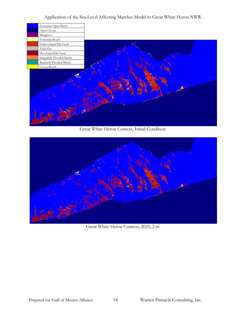
Great White Heron Context, Initial Condition
Estuarine Open WaterEstuarine Open WaterOpen Ocean
MangroveMangrove
Estuarine BeachEstuarine BeachUndeveloped Dry Land
Tidal Fla tTidal Flat
Developed Dry LandDeveloped Dry Land
Irregularly Flooded MarshIrregularly Flooded Marsh
R egularly Flooded MarshRegularly Flooded Marsh
Ocean BeachOcean Beach
Undeveloped Dry Land
Great White Heron Context, 2025, Scenario A1B Mean
Prepared for Gulf of Mexico Alliance 42 Warren Pinnacle Consulting, Inc.

Application of the Sea-Level Affecting Marshes Model to Great White Heron NWR
Great White Heron Context, 2050, Scenario A1B Mean
Great White Heron Context, 2075, Scenario A1B Mean
Prepared for Gulf of Mexico Alliance 43 Warren Pinnacle Consulting, Inc.
Application of the Sea-Level Affecting Marshes Model to Great White Heron NWR
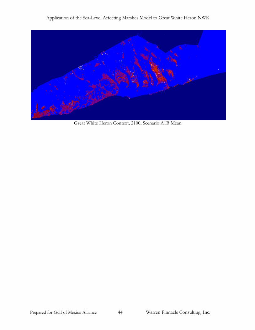
Great White Heron Context, 2100, Scenario A1B Mean
Prepared for Gulf of Mexico Alliance 44 Warren Pinnacle Consulting, Inc.

Application of the Sea-Level Affecting Marshes Model to Great White Heron NWR
Great White Heron Context, Initial Condition, 2009
Estuarine Open WaterEstuarine Open WaterOpen Ocean
MangroveMangrove
Estuarine BeachEstuarine BeachUndeveloped Dry Land
Tidal Fla tTidal Flat
Developed Dry LandDeveloped Dry Land
Irregularly Flooded MarshIrregularly Flooded Marsh
R egularly Flooded MarshRegularly Flooded Marsh
Ocean BeachOcean Beach
Undeveloped Dry Land
Great White Heron Context, 2025, Scenario A1B Maximum
Prepared for Gulf of Mexico Alliance 45 Warren Pinnacle Consulting, Inc.

Application of the Sea-Level Affecting Marshes Model to Great White Heron NWR
Great White Heron Context, 2050, Scenario A1B Maximum
Great White Heron Context, 2075, Scenario A1B Maximum
Prepared for Gulf of Mexico Alliance 46 Warren Pinnacle Consulting, Inc.

Application of the Sea-Level Affecting Marshes Model to Great White Heron NWR
Great White Heron Context, 2100, Scenario A1B Maximum
Prepared for Gulf of Mexico Alliance 47 Warren Pinnacle Consulting, Inc.

Application of the Sea-Level Affecting Marshes Model to Great White Heron NWR
Great White Heron Context, Initial Condition
Estuarine Open WaterEstuarine Open WaterOpen Ocean
MangroveMangrove
Estuarine BeachEstuarine BeachUndeveloped Dry Land
Tidal Fla tTidal Flat
Developed Dry LandDeveloped Dry Land
Irregularly Flooded MarshIrregularly Flooded Marsh
R egularly Flooded MarshRegularly Flooded Marsh
Ocean BeachOcean Beach
Undeveloped Dry Land
Great White Heron Context, 2025, 1 m
Prepared for Gulf of Mexico Alliance 48 Warren Pinnacle Consulting, Inc.

Application of the Sea-Level Affecting Marshes Model to Great White Heron NWR
Great White Heron Context, 2050, 1 m
Great White Heron Context, 2075, 1 m
Prepared for Gulf of Mexico Alliance 49 Warren Pinnacle Consulting, Inc.
Application of the Sea-Level Affecting Marshes Model to Great White Heron NWR
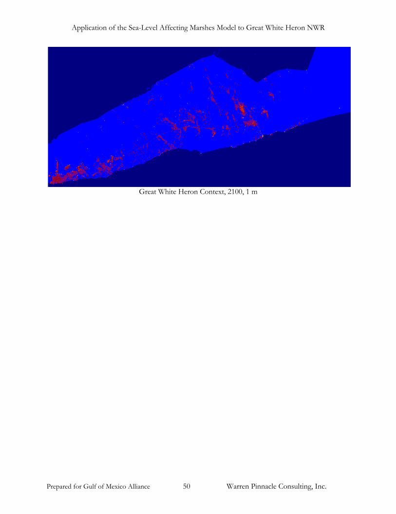
Great White Heron Context, 2100, 1 m
Prepared for Gulf of Mexico Alliance 50 Warren Pinnacle Consulting, Inc.

Application of the Sea-Level Affecting Marshes Model to Great White Heron NWR
Great White Heron Context, Initial Condition
Estuarine Open WaterEstuarine Open WaterOpen Ocean
MangroveMangrove
Estuarine BeachEstuarine BeachUndeveloped Dry Land
Tidal Fla tTidal Flat
Developed Dry LandDeveloped Dry Land
Irregularly Flooded MarshIrregularly Flooded Marsh
R egularly Flooded MarshRegularly Flooded Marsh
Ocean BeachOcean Beach
Undeveloped Dry Land
Great White Heron Context, 2025, 1.5 m
Prepared for Gulf of Mexico Alliance 51 Warren Pinnacle Consulting, Inc.

Application of the Sea-Level Affecting Marshes Model to Great White Heron NWR
Great White Heron Context, 2050, 1.5 m
Great White Heron Context, 2075, 1.5 m
Prepared for Gulf of Mexico Alliance 52 Warren Pinnacle Consulting, Inc.

Application of the Sea-Level Affecting Marshes Model to Great White Heron NWR
Great White Heron Context, 2100, 1.5 m
Prepared for Gulf of Mexico Alliance 53 Warren Pinnacle Consulting, Inc.
Application of the Sea-Level Affecting Marshes Model to Great White Heron NWR
Great White Heron Context, Initial Condition
Estuarine Open WaterEstuarine Open WaterOpen Ocean
MangroveMangrove
Estuarine BeachEstuarine BeachUndeveloped Dry Land
Tidal Fla tTidal Flat
Developed Dry LandDeveloped Dry Land
Irregularly Flooded MarshIrregularly Flooded Marsh
R egularly Flooded MarshRegularly Flooded Marsh
Ocean BeachOcean Beach
Undeveloped Dry Land
Great White Heron Context, 2025, 2 m
Prepared for Gulf of Mexico Alliance 54 Warren Pinnacle Consulting, Inc.

Application of the Sea-Level Affecting Marshes Model to Great White Heron NWR
Great White Heron Context, 2050, 2 m
Great White Heron Context, 2075, 2 m
Prepared for Gulf of Mexico Alliance 55 Warren Pinnacle Consulting, Inc.

Application of the Sea-Level Affecting Marshes Model to Great White Heron NWR
Prepared for Gulf of Mexico Alliance 56 Warren Pinnacle Consulting, Inc.
Great White Heron Context, 2100, 2 m