application of the new keynesian phillips curve inflation ... · ˜˚˛˜˝˙ˆˇ˘ˇ ˇ˝ ˙ ˜˝...

ASIAN DEVELOPMENT BANK

AsiAn Development BAnk6 ADB Avenue, Mandaluyong City1550 Metro Manila, Philippineswww.adb.org

Application of the New Keynesian Phillips Curve Inflation Model in Sri Lanka

This working paper applied the New Keynesian Phillips Curve (NKPC) framework to nonfood inflation in Sri Lanka during January 2006-April 2015. It differs from other papers on NKPC in three ways: (i) inflation defined as a month-on-month increase in the price index to avoid base effect; (ii) monthly output gap is estimated from power generation data to ensure sufficient number of data for regressions; and (iii) nominal effective exchange rate, global commodity prices, and domestic fuel prices are included into explanatory variables to capture supply-side impact on prices. With all these features, the paper confirmed that the forward-looking NKPC model is applicable to Sri Lanka.

About the Asian Development Bank

ADB’s vision is an Asia and Pacific region free of poverty. Its mission is to help its developing member countries reduce poverty and improve the quality of life of their people. Despite the region’s many successes, it remains home to the majority of the world’s poor. ADB is committed to reducing poverty through inclusive economic growth, environmentally sustainable growth, and regional integration.

Based in Manila, ADB is owned by 67 members, including 48 from the region. Its main instruments for helping its developing member countries are policy dialogue, loans, equity investments, guarantees, grants, and technical assistance.

APPLICAtIoN of the New KeyNeSIAN PhILLIPS Curve INfLAtIoN MoDeL IN SrI LANKATadateru Hayashi, Nimali Hasitha Wickremasinghe, and Savindi Jayakody

adb SOUTH aSia wOrking paper SerieS

No. 36

august 2015

.c

ADB South Asia Working Paper Series


Tadateru Hayashi

Nimali Hasitha Wickremasinghe

Savindi Jayakody

No. 36 August 2015

Tadateru Hayashi is Senior Country Economist. Nimali Hasitha Wickremasinghe is Senior Economics Officer, and Savindi Jayakody is Economics Analyst at the Sri Lanka Resident Mission of the Asian Development Bank.


Asian Development Bank 6 ADB Avenue, Mandaluyong City 1550 Metro Manila, Philippines www.adb.org © 2015 by Asian Development Bank August 2015 ISSN 2313-5867 (Print), 2313-5875 (e-ISSN) Publication Stock No. WPS157526-2 The views expressed in this publication are those of the author and do not necessarily reflect the views and policies of the Asian Development Bank (ADB) or its Board of Governors or the governments they represent. ADB does not guarantee the accuracy of the data included in this publication and accepts no responsibility for any consequence of their use. By making any designation of or reference to a particular territory or geographic area, or by using the term “country” in this document, ADB does not intend to make any judgments as to the legal or other status of any territory or area. ADB encourages printing or copying information exclusively for personal and noncommercial use with proper acknowledgment of ADB. Users are restricted from reselling, redistributing, or creating derivative works for commercial purposes without the express, written consent of ADB. Unless otherwise noted, “$” refers to US dollars. Printed on recycled paper

The ADB South Asia Working Paper Series is a forum for ongoing and recently completed research and policy studies undertaken in ADB or on its behalf. It is meant to enhance greater understanding of current important economic and development issues in South Asia, promote policy dialogue among stakeholders, and facilitate reforms and development management. The ADB South Asia Working Paper Series is a quick-disseminating, informal publication whose titles could subsequently be revised for publication as articles in professional journals or chapters in books. The series is maintained by the South Asia Department. The series will be made available on the ADB website and on hard copy.

CONTENTS

1. INTRODUCTION .................................................................................................................................................. 1

2. BACKGROUND ................................................................................................................. .................................... 1

3. NEW KEYNESIAN PHILLIPS CURVE (NKPC) ......................................................................................... 4

4. DATA AND METHODOLOGY ...................................................................................................................... 6

5. REGRESSION RESULTS .................................................................................................................................... 13

6. CONCLUSIONS AND NEXT STEPS .......................................................................................................... 17

REFERENCES ........................................................................................................................................................ 18

TABLES AND FIGURES

TABLES

1. Correlation between GDP growth and Power Generation Growth (quarterly) .............................. 9

2. Forward-Looking Model with Month-on-Month Data ......................................................................... 14

3. Backward-Looking Model with Month-on-Month Data ...................................................................... 14

4. Forward Looking Model with Year-on-Year Data ....................................................................................15

5. Backward Looking Model with Year-on-Year Data .................................................................................15

6. Detailed Regression Results of Selected Forward-looking Model ..................................................... 16

7. Detailed Regression Results of Selected Backward-looking Model .................................................. 17

FIGURES

1. Inflation in Sri Lanka (year-on-year) .............................................................................................................. 2

2. Policy Rates .............................................................................................................................................................. 3

3. Overall Inflation ...................................................................................................................................................... 7

4. Nonfood Inflation .................................................................................................................................................. 7

5. Base Effect of Permanent Shock ...................................................................................................................... 8

6. Base Effect of Temporary Shock ...................................................................................................................... 8

7. Power Generation Gap and GDP Gap ......................................................................................................... 10

8. NEER and Deviation from its Trend ............................................................................................................... 11

9. All Commodity Prices Index and Deviation from its Trend ................................................................... 11

10. Price of Lanka Auto Diesel and deviation from its Trend ...................................................................... 12

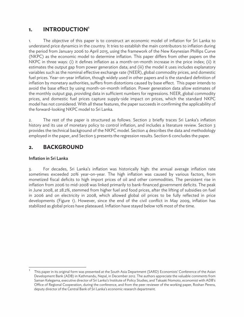
1. INTRODUCTION1 1. The objective of this paper is to construct an economic model of inflation for Sri Lanka to understand price dynamics in the country. It tries to establish the main contributors to inflation during the period from January 2006 to April 2015, using the framework of the New Keynesian Phillips Curve (NKPC) as the economic model to determine inflation. This paper differs from other papers on the NKPC in three ways: (i) it defines inflation as a month-on-month increase in the price index; (ii) it estimates the output gap from power generation data; and (iii) the model it uses includes explanatory variables such as the nominal effective exchange rate (NEER), global commodity prices, and domestic fuel prices. Year-on-year inflation, though widely used in other papers and is the standard definition of inflation by monetary authorities, suffers from distortions caused by base effect. This paper intends to avoid the base effect by using month-on-month inflation. Power generation data allow estimates of the monthly output gap, providing data in sufficient numbers for regressions. NEER, global commodity prices, and domestic fuel prices capture supply-side impact on prices, which the standard NKPC model has not considered. With all these features, the paper succeeds in confirming the applicability of the forward-looking NKPC model to Sri Lanka. 2. The rest of the paper is structured as follows. Section 2 briefly traces Sri Lanka’s inflation history and its use of monetary policy to control inflation, and includes a literature review. Section 3 provides the technical background of the NKPC model. Section 4 describes the data and methodology employed in the paper, and Section 5 presents the regression results. Section 6 concludes the paper. 2. BACKGROUND Inflation in Sri Lanka 3. For decades, Sri Lanka’s inflation was historically high: the annual average inflation rate sometimes exceeded 20% year-on-year. The high inflation was caused by various factors, from monetized fiscal deficits to high import prices of oil and other commodities. The persistent rise in inflation from 2006 to mid-2008 was linked primarily to bank-financed government deficits. The peak in June 2008, at 28.2%, stemmed from higher fuel and food prices, after the lifting of subsidies on fuel in 2006 and on electricity in 2008, which allowed global oil prices to be fully reflected in price developments (Figure 1). However, since the end of the civil conflict in May 2009, inflation has stabilized as global prices have plateaued. Inflation have stayed below 10% most of the time.

1 This paper in its original form was presented at the South Asia Department (SARD) Economists’ Conference of the Asian

Development Bank (ADB) in Kathmandu, Nepal, in December 2012. The authors appreciate the valuable comments from Saman Kelegama, executive director of Sri Lanka’s Institute of Policy Studies, and Takaaki Nomoto, economist with ADB’s Office of Regional Cooperation, during the conference, and from the peer reviewer of the working paper, Roshan Perera, deputy director of the Central Bank of Sri Lanka’s economic research department.

2 ADB South Asia Working Paper Series No. 36

4. Inflation in Sri Lanka is measured in terms of percentage changes in the Colombo Consumer Price Index (CCPI). A CCPI with 2006/2007 as base year is available for the period from January 2008 to the present, and a CCPI with a 2002 base year is available for January 2003 to May 2011. The base year was changed to reflect the development of consumer patterns, and weights for the various categories were revised accordingly. Food and nonalcoholic beverages, whose prices have been far more volatile than those of other items, have declined in significance, from 46.7% in the 2002 base-year series to 41.0% in the 2006/2007 base-year series. On the other hand, housing, water, electricity, gas, and other fuels have gained in relative importance, from 18.3% to 23.7%, as has transport, from 9.5% to 12.3%. Monetary Policy 5. Price stability is the final target of monetary policy in Sri Lanka. The Central Bank of Sri Lanka (CBSL) manages inflation within a monetary targeting framework, and it maintains price stability with reserve money as the operating target and broad money as the intermediate monetary policy target. Monetary policy instruments have gradually moved toward more market-oriented measures. They are now focused more on open market operations and less on the statutory reserve requirement. The CBSL signals its monetary policy stance through the standing deposit facility rate (formerly known as the repurchase, or repo, rate) and the standing lending facility rate (formerly, the reverse repurchase, or reverse repo, rate), while buying and selling Treasury bills (T-bills) to manage market liquidity in line with the reserve money target. During the high-inflation period from 2006 to mid-2008, the CBSL maintained a tight monetary policy stance and revised its reserve money (M0) growth targets on three occasions, making them more stringent to hold down rising inflationary pressures. The annual average reserve money growth target was brought down from 14.7% to 9.7% in three steps. The CBSL also raised policy rates (standing deposit/lending facility rates) nine times in 2005–2007 to contain the price hike (Figure 2).

Figure 1: Inflation in Sri Lanka (year-on-year)

Source: Central Bank of Sri Lanka.

Application of New Keynesian Phillips Curve Inflation Model in Sri Lanka 3

6. Supply-side shocks such as weather conditions (through agriculture product prices), domestic energy prices, and import prices (through fluctuations in international market prices and in the foreign exchange rate), in addition to demand-side factors, have had inflationary effects. The Sri Lankan rupee floats within a preannounced band, which has been increasingly broadened over the years. In January 2001, the CBSL liberalized the foreign exchange market, moving away from buying or selling foreign exchange at preannounced rates. Commercial banks were instead allowed to determine exchange rates, with the CBSL monitoring movements and reserving the right to intervene in the market to smoothing short term volatility. In 2011, the rupee came under pressure as the CBSL defended the currency despite external imbalances and lost 27% of external reserves between mid-August and end-December 2011. The CBSL changed its foreign exchange policy in February 2012 and announced that it would limit its intervention in the foreign exchange market, and move toward greater market determination of the exchange rate. Domestic energy prices (both electricity tariff and fuel prices) are administered by the government. More recently, both power tariff and fuel prices were decreased in September 2014. Fuel prices were further cut in December 2014 and again substantially in January 2015. Literature Review 7. A number of studies have investigated the determinants of inflation in Sri Lanka. Ratnasiri (2009) attempted to identify the main determinants of inflation in Sri Lanka in 1980–2005 through vector autoregressive (VAR) analysis. The study used five variables to test the impact on inflation: the output gap derived from seasonally adjusted log-form gross domestic product (GDP) using the Hodrick–Prescott (HP) filter, money supply (M2), rice price (point-to-point growth), interest rate (91-day T-bill yield), and exchange rate depreciation (quarter-on-quarter growth). Ratnasiri concluded that money supply and rice price drive inflation in the long run, while exchange rate depreciation and output gap have no statistically significant effects on inflation. In addition, using a vector error

Figure 2: Policy Rates



correction model, Ratnasiri showed that rice price is the most important determinant in the short run, but money supply growth and exchange rate are not so important. Output gap has no significant effect on short-run inflation. Since the price of rice is the most significant determinant in both the short and the long run, and food carried over 60% weight in the price index at that time, the paper recommended increasing the supply of rice to reduce inflation. 8. Amarasekara (2008) also used a VAR framework in analyzing the effects of interest rate, money growth, and movements in nominal exchange rate on real GDP growth and inflation. His study used both recursive structures and semistructural VARs with quarterly GDP, CCPI, the special drawing rights (SDR) exchange rate, reserve money, and the interbank call rate—all of them seasonally adjusted. The study confirmed that higher interest rates reduce GDP growth and inflation, and increase the exchange rate. The effect on GDP, however, contrasts with established findings when money growth and exchange rate are the policy variables. Inflation also does not decrease following a contractionary policy shock, because of a longer lag effect, according to Amarasekara. 9. Harischandra (2007) examined the effects of monetary policy and inflation performance across exchange rate regimes in Sri Lanka. The degree of inflation persistence was used as the criterion to examine inflation performance in three alternative definitions: (i) positive serial correlation in inflation (type 1 inflation persistence); (ii) lags between systematic monetary policy actions and their (peak) effects on inflation (type 2); and (iii) lagged response to nonsystematic policy actions—policy shocks (type 3). Harischandra used the autocorrelation coefficient of the price inflation process and different specifications of the Phillips curve in examining type 1 inflation persistence, correlations between monetary policy measures and consumer price inflation for type 2, and impulse response analysis for type 3. Evidence of an upward shift in inflation persistence between regimes was confirmed for type 1, and a significant lag between the peak effect on inflation and a change in monetary policy, for type 2. Inflation has been more persistent under a flexible exchange-rate regime. For type 3 inflation persistence, the assessment showed that the effects of a policy shock are less sustained under a fixed regime. Inflation response to changes in interest rate, however, provides only weak evidence. 10. Despite advances in the theoretical modeling of inflation, econometric analysis of the NKPC for Sri Lanka has been limited. Anand, Ding, and Peiris (2011) developed a forecasting model–based simultaneous equation system including NKPC. Their findings implied that open-economy inflation targeting can reduce macroeconomic volatility and anchor inflationary expectations, given the size and type of shocks faced by the economy. In addition, monetary policy rules can help guide the authority in taking the appropriate monetary stance. 3. THE NEW KEYNESIAN PHILLIPS CURVE 11. The NKPC depends on two sets of microeconomic foundations: monopolistic competitive firms and sticky prices. In monopolistic competition, each differentiated good is produced by one firm, which determines the price of the good it produces. Although the goods are different, some degree of supplementarity is assumed. Therefore, competition among goods still exists. 12. Sticky prices arise from a constraint on price adjustment by firms. Calvo (1983) assumed that only some firms are able to change the prices of their products within a given period. The likelihood of a change in price is independent of the last adjustment. The aggregate price in a given period will therefore be a weighted average of the adjusted price and the price in the previous period. This stickiness in prices is due to the cost of price adjustment (often called the “menu cost”) and long-term contracts to provide goods at fixed prices.


13. Under these assumptions, firms set the prices of their goods by adding a markup to the nominal marginal cost to maximize their medium- to long-term profits. Given the constraints on the timing of price adjustments and the availability of information needed to forecast future marginal costs, the aggregate price will be determined through the following equation:

t = Ett+n + rmct (1)

where t is the inflation rate in the period t, Ett+n is the expected inflation of period t+n in the period t, and rmct is the deviation of real marginal cost from its steady state in the period t.

14. Equation (1) describes the NKPC. The coefficient indicates the degree of price stickiness. If more firms adjust their prices, will be larger, that is, inflation will be determined to a greater extent by real marginal cost. 15. An increase or a decrease in real marginal cost is closely linked to the output gap. When monetary accommodation increase the nominal aggregate demand under full employment, since the aggregate price is sticky, real aggregate demand will increase. Firms will increase production beyond the full employment level as a result of their profit maximization behavior, and hence generate a positive output gap. Thus, if a perfect labor market (flexible nominal wage, no cost for labor adjustment, and no mismatch between labor demand and supply) were assumed, there will be a linear relationship between the output gap and the real marginal cost. In the light of this relationship, equation (1) can be transformed into equation (2) below. While some papers such as those of Galí and Gertler (1999) and Galí, Gertler, and López-Salido (2001) suggest that NKPC based on marginal cost provides a better fit than NKPC based on output gap, equation (2) is widely used in empirical studies because firms’ marginal cost data are not always available. For the same reason, this paper also uses equation (2) as the baseline model for Sri Lanka.

t = Ett+n + gapt (2)

where gapt is the output gap in period t.

16. The NKPC has been criticized for not capturing supply-side shocks, such as the impact of import prices and fuel prices. In fact, the exchange rate could affect inflation through its direct impact on import prices. Within the microeconomic framework of NKPC, supply shocks can be considered to impact the inflation through change in markup by firms. Batinia, Jackson, and Nickell (2005) provided empirical evidence that inflation in UK is explained by changes in both employment and real import prices in general, and in real oil prices in particular. Ho and McCauley (2003) suggested that the significance of the exchange rate in the evolution of domestic inflation tends to be greater for emerging market economies than for developed economies. Sahu (2013) used an open-economy model for India over the period 1996/97 to 2009/10 and found that fuel inflation, exchange rate and foreign inflation are significant determinants of India’s inflation. The supply-side shocks can be captured by additional explanatory variables representing the shocks as in equation (3).

t = Ett+n + gapt + supply-side shocks (3) 17. It is known that, for many empirical studies, the NKPC model is not always a good fit. In many instances, therefore, inflation dynamics has been alternatively defined in terms of a hybrid NKPC, where inflation is governed by a combination of forward-looking inflation expectations and lagged inflation, which represents backward-looking price-setting behavior. The hybrid NKPC adds lagged


inflation as an explanatory variable, as in equation (4).2 The challenge presented by the hybrid model stems from the fact that the microeconomic foundations under the NKPC framework do not explain the persistence of inflation. Galí and Gertler (1999) suggested that inflation inertia could result from sluggish adjustment of real marginal costs to movements in output. It was pointed out that, because of information constraints, some firms could base their marginal costs on recent aggregate price which generates the backward looking behavior. After isolating the factors that drive real marginal costs, Galí, Gertler, and López-Salido (2001) showed that labor market frictions are likely to have had a key role in the evolution of real marginal costs, both in the euro area and in the US, and suggested that those frictions may help explain inflation persistence in both cases. But in the absence of a consensus to explain the persistence of this behavior, the rationale for the hybrid approach remains largely empirical.

t = Ett+n + gapt + supply-side shocks + t-1 (4) 4. DATA AND METHODOLOGY 18. A single series of inflation was prepared for the period from January 2006 to April 2015.3 The ratio between the CCPI for base year 2006/2007 and that for base year 2002 is almost fixed at 0.63 for the period when both CCPIs exist. Therefore, the 2002 base year inflation series between January 2006 and December 2007 was multiplied by 0.63, and treated as continuous data of 2006/2007 series. Among the categories in the CCPI consumption basket, food and beverage prices are vulnerable to supply-side shocks such as weather conditions and thus fluctuate widely. But they also reflect demand-side factors, which are difficult to separate from supply-side factors. Therefore, this paper excludes the food and beverage component from the price index and deals instead with nonfood inflation. Thus, in the rest of the paper, inflation refers to nonfood inflation unless otherwise specified. 19. Inflation is calculated in two different ways: year-on-year and month-on-month. Year-on-year inflation is the standard definition of inflation and measures the increase in the CCPI over the same month the previous year. On the other hand, month-on-month inflation measures the increase in the CCPI over the previous month. To obtain month-on-month inflation, the CCPI for items was first seasonally adjusted with the help of the X13-ARIMA Seasonal Adjustment Program, and the monthly increase was then calculated. In view of the rather large fluctuations in the month-on-month inflation rate, the 3-month moving average was used for regressions in this paper.

2 The explanatory variable representing supply-side shock is not an essential part of the hybrid NKPC. 3 The starting time correspond to the available output gap proxy data (to be explained later on in this paper).


Figure 3: Overall Inflation


Figure 4: Nonfood Inflation



20. Month-on-month inflation has the advantage of avoiding disturbances from the base effect. The examples below show the base-effect distortion in the case of permanent and temporary shocks. Following a permanent downward shock in February 2015, a price index that has been increasing by 0.5% monthly, or by 6.2% annually, will undergo a parallel downward shift, and will follow its previous rising trend from March 2015 at the lower level (Figure 5). Month-on-month inflation will be lower in the month of the shock, but will go up to its previous rate in the succeeding months. Year-on-year inflation, on the other hand, will go down not only in the month of the shock but also in the next 12 months (until February 2016). This is a base effect. Note that year-on-year inflation finally rises again in March 2016, but there is no change takes place in the price index in the month. Year-on-year inflation jumps back in March 2016 only because the price index for the month is compared with that for the same month a year ago. In case of a temporary shock, as indicated in Figure 6, the price index will resume its previous trend in the next month after the shock in February 2015. Month-on-month inflation will drop in February 2015, and rebounds immediately after in March 2015, indicating that prices have again taken up their previous level. Year-on-year inflation will also goes back to the previous rate immediately in March 2015. Note that year-on-year inflation jumps after 12 months in March 2016, although there is no major surge in price level. This is also a base effect from the drop in price level a year ago.

Figure 5: Base Effect of Permanent Shock

Source: Prepared by ADB staff.

Figure 6: Base Effect of Temporary Shock



21. Inflation expectation (t+n) is represented by actual inflation in the future at the time of expectation. For example, actual inflation in December 2014 is used as 6 months ahead inflation expectation at the time of June 2014. This assumes that people can perfectly predict inflation. The letter n stands for the number of months ahead of the time when the inflation forecast is made. 22. Output gap (gapt) is the deviation of actual output from the natural (or potential) output level. At the natural level of output, it is assumed that all production input is fully used. Output gap is estimated from GDP data, but since GDP data are usually available only quarterly, the sample is often limited, and obtaining a decent regression results is a challenge. In the case of Sri Lanka, GDP data at constant 2002 prices were available only from the first quarter of 2002 to the fourth quarter of 2014 at the time this paper was prepared. Available data covered only 48 quarters. To address this issue, this paper uses power generation data in estimating the output gap. Power generation data have the advantage of being available monthly. In addition, power generation in general closely correlates with GDP, as electricity is a basic economic input. Table 1 shows that (quarterly) power generation growth in Sri Lanka has had a strong positive correlation with GDP growth (both in year-on-year) since 2006, except in 2010 when the economy slowed down. Before 2006, however, the correlation was weak. Therefore, this paper uses the monthly power generation gap since January 2006 as a proxy for output gap in this paper.

Table 1: Correlation between GDP growth and Power Generation Growth (Quarterly)

Period Correlation2003 -0.682004 -0.242005 -0.212006 0.802007 0.852008 0.742009 0.972010 -0.952011 0.682012 0.942013 0.482014 0.45

2006-2014 0.76Jul 2009-Dec 2014 0.65



23. The standard methodology to estimate output gap was applied to the power generation to calculate the output gap. First, seasonal changes were removed from the total power generation data for January 2006 to December 2014, by means of the X13-ARIMA Seasonal Adjustment Program. Then the natural log of the seasonally adjusted series was taken, and its trend was obtained with the HP filter (with = 14,400). The deviation of the natural log of the seasonally adjusted series from its trend was the estimated output gap. For comparison, the same procedure was followed in estimating the output gap from quarterly GDP data—the data were seasonally adjusted, the natural log was taken, and the difference between the natural log and its HP-filtered trend (with = 1,600) was determined. The estimated gaps are shown in Figure 7.

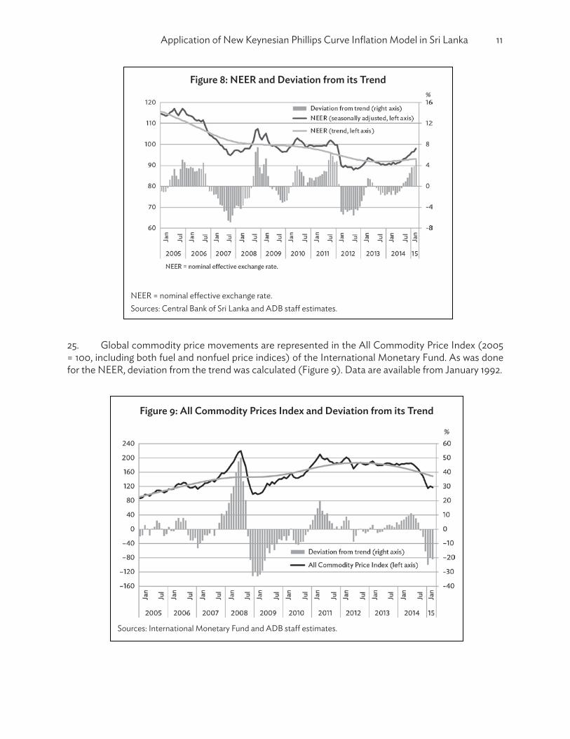
24. The nominal effective exchange rate (NEER) is an index of a weighted average of a country’s foreign exchange rates with its major trading partners. The deviation of the seasonally adjusted series from its HP-filtered trend (neert) was used as a data series to indicate supply-side shocks (Figure 8) on the assumption that large and fast movements in the foreign exchange rate can affect domestic inflation through import prices. In fact, the Sri Lankan rupee has depreciated heavily several times in the past decade, and was floated on one such occasion in early 2012. The NEER for Sri Lanka is available for the period since January 2003.

Figure 7: Power Generation Gap and GDP Gap

Note: Quarterly GDP gap is used for the corresponding months. Sources: Department of Census and Statistics, Ceylon Electricity Board, and ADB staff estimates.


25. Global commodity price movements are represented in the All Commodity Price Index (2005 = 100, including both fuel and nonfuel price indices) of the International Monetary Fund. As was done for the NEER, deviation from the trend was calculated (Figure 9). Data are available from January 1992.

Figure 8: NEER and Deviation from its Trend

NEER = nominal effective exchange rate. Sources: Central Bank of Sri Lanka and ADB staff estimates.

Figure 9: All Commodity Prices Index and Deviation from its Trend

Sources: International Monetary Fund and ADB staff estimates.


26. Sri Lanka’s domestic fuel prices are represented by the price of Lanka Auto Diesel (retail price for 1 liter). Data are available from March 1990. The price, its trend, and deviations from the trend are shown in Figure 10.

27. Finally, the hybrid NKPC model includes inflation in the past—this paper uses inflation data with a 1-month lag (t–1) in regressions. 28. The NKPC models in this paper are those obtained through equations (3) and (4).4 Regressions were undertaken for both month-on-month and year-on-year inflation as dependent variables. The regressions were generated in eight variations depending on the explanatory variables for supply-side shocks: with or without the NEER, with or without global commodity prices, and with or without domestic fuel prices. Inflation expectations ranged from 1 to 32 months ahead. Finally, 1-month lagged inflation was added as an explanatory variable to each of the above models to test the hybrid NKPC model. The regressions first used the full data set for January 2006–April 2015, and then with postconflict data for July 2009–April 2015 to check the robustness of the regression results.

4 Equation (2) and its hybrid version were also used.

Figure 10: Price of Lanka Auto Diesel and deviation from its Trend

Sources: Ceylon Petroleum Corporation and ADB staff estimates.


29. The generalized method of moments (GMM) was used in undertaking the regressions, as the NKPC model includes a lagged dependent variable as explanatory variable (lags to the future, and to the past in the case of the hybrid model). The 1-month-before data of the lagged dependent variables were used as instrumental variables, that is, t+n–1 was used as instrumental variable for t+n, and t–2 for t–1. 30. The coefficients are expected to have a positive sign for inflation expectation (t+n), output gap (gapt), backward-looking inflation (t–1), global commodity prices (gcpt), and domestic fuel prices (fuelt), and negative for the deviation of NEER from its trend (neert). 5. REGRESSION RESULTS 31. Tables below summarize the regression results for forward-looking and backward-looking models, with month-on-month inflation (Tables 2 and 3) or year-on-year inflation (Tables 4 and 5) as dependent variable. Group A does not include any variable for supply-side shocks. Group B has NEER; group C, global commodity prices; group D, domestic fuel prices; group E, NEER and global commodity prices; group F, NEER and domestic fuel prices; group G, global commodity prices and domestic fuel prices; and group H, all three supply-side variables. Each box in the tables represents a regression result. If all of the coefficients in the regression are at least at 1% significance level with the expected sign, the box is marked with “***”. If one or more coefficients is at 5% or 10% significance level, the box has a “**” or “*” mark, respectively. If the significance level of one of the coefficients is below 10%, or one of the coefficients has the wrong sign, the box is unmarked. The regression results with full data are shown at the top of the boxes. Regression results with postconflict data (July 2009 onward) are in the second row of the boxes under “sensitivity test.” If the regression with full data generated significant results, endogeneity test and weak instrument diagnostics (WID) test were performed, and the third and fourth rows were added to the boxes—the third row showing the significance level of the differences in J-statistics of the endogeneity test, and the fourth row showing a “*” if the Cragg–Donald F-statistic is larger than the Stock–Yogo critical value at 10% level. Regressions with significant results, with all the tests passed, are highlighted (three boxes in Table 2 and two boxes in Table 5).


Table 2: Forward-Looking Model with Month-on-Month Data

*** = all coefficients are significant at 1% level, with the expected sign; ** = one or more coefficients are significant at 5% level, with all coefficients having the expected sign; * = one or more coefficients are significant at 10% level, with all coefficients having the expected sign; – = no diagnostic test undertaken because regression results were not significant; WID = weak instrumental diagnostics; reg = regression. Source: ADB staff estimates.

Table 3: Backward-Looking Model with Month-on-Month Data

*** = all coefficients are significant at 1% level, with the expected sign; ** = one or more coefficients are significant at 5% level, with all coefficients having the expected sign; * = one or more coefficients are significant at 10% level, with all coefficients having the expected sign; – = no diagnostic test undertaken because regression results were not significant; WID = weak instrument diagnostics; reg = regression. Source: ADB staff estimates.











*** = all coefficients are significant at 1% level, with the expected sign; ** = one or more coefficients are significant at 5% level, with all coefficients having the expected sign; * = one or more coefficients are significant at 10% level, with all coefficients having the expected sign; – = no diagnostic test undertaken because regression results were not significant; WID = weak instrumental diagnostics; reg = regression.

Source: ADB staff estimates.

*** = all coefficients are significant at 1% level, with the expected sign; ** = one or more coefficients are significant at 5% level, with all coefficients having the expected sign; * = one or more coefficients are significant at 10% level, with all coefficients having the expected sign; – = no diagnostic test undertaken because regression results were not significant; WID = weak instrument diagnostics; reg = regression.













Table 4: Forward-Looking Model with Year-on-Year Data

*** = all coefficients are significant at 1% level, with the expected sign; ** = one or more coefficients are significant at 5% level, with all coefficients having the expected sign; * = one or more coefficients are significant at 10% level, with all coefficients having the expected sign; reg = regression. Source: ADB staff estimates.

Table 5: Backward-Looking Model with Year-on-Year Data












*** = all coefficients are significant at 1% level, with the expected sign; ** = one or more coefficients are significant at 5% level, with all coefficients having the expected sign; * = one or more coefficients are significant at 10% level, with all coefficients having the expected sign; reg = regression.












*** = all coefficients are significant at 1% level, with the expected sign; ** = one or more coefficients are significant at 5% level, with all coefficients having the expected sign; * = one or more coefficients are significant at 10% level, with all coefficients having the expected sign; – = no diagnostic test undertaken because regression results were not significant; WID = weak instrument diagnostics; reg = regression.



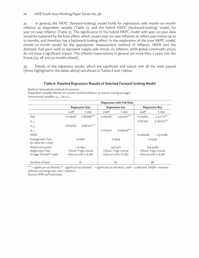
32. In general, the NKPC (forward-looking) model holds for regressions with month-on-month inflation as dependent variable (Table 2), and the hybrid NKPC (backward-looking) model, for year-on-year inflation (Table 5). The significance of the hybrid NKPC model with year-on-year data would be explained by the base effect, which causes year-on-year inflation, to reflect past events up to 12 months, and therefore has a backward-looking effect. In the exploration of the pure NKPC model, month-on-month would be the appropriate measurement method of inflation. NEER and the domestic fuel price work to represent supply-side shocks on inflation, while global commodity prices do not have a significant impact. The inflation expectations in general are more than 2 years into the future (23, 28, and 30 months ahead). 33. Details of the regression results, which are significant and robust with all the tests passed (those highlighted in the tables above) are shown in Tables 6 and 7 below.

Table 6: Detailed Regression Results of Selected Forward-looking Model Method: Generalized method of moments Dependent variable: Month-on-month nonfood inflation (3-month moving average) Instrumental variable: t+n–1 for t+n

Regression with Full Data Regression A30 Regression A31 Regression B23

coeff t-stat coeff t-stat coeff t-statGap 0.155158 3.681898*** 0.165266 3.919297*** 0.093815 2.417713**t+23 0.657501 5.139032***t+30 0.675007 3.990301*** t+31 0.703192 3.295304*** NEER –0.084286 –2.912086Endogeneity Test (p-value for J-stat)

0.0960 0.0634 0.0304

Weak Instrument Diagnostics Test (Cragg–Donald F-stat)

175.1852(Stock–Yogo critical value at 10% is 16.38)


209.9085 (Stock–Yogo critical value at 10% is 16.38)

Number of data 81 80 88

*** = significant at 1% level, ** = significant at 5% level, * = significant at 10% level, coeff = coefficient, NEER = nominal effective exchange rate, stat = statistics. Source: ADB staff estimates.


Table 7 : Detailed Regression Results of Selected Hybrid Backward-looking Model Method: Generalized method of moments Dependent variable: Year-on-year nonfood inflation (3-month moving average) Instrumental variables: t+n–1 for t+n, and t-2 for t–1.

Regression with Full Data Regression B28 Regression F28

Coeff t-stat Coeff t-stat Gap 0.152242 2.086890** 0.158456 2.270030**

t+28 0.067327 2.876811*** 0.101113 3.698220***

NEER –0.101412 –2.563490** –0.074202 –1.992298**

FUEL 0.947815 41.58477*** 0.044454 3.324648***

t-1 0.920067 47.27780***

Endogeneity Test (p-value for J-stat)

0.0392 0.0817

Weak Instrument Diagnostics Test (Cragg–DonaldF-stat)


342.9543 (Stock–Yogo critical value at 10% is 7.03)

Number of data 82 82

*** = significant at 1% level, ** = significant at 5% level, * = significant at 10% level, coeff = coefficient, FUEL = price of Lanka Auto Diesel (retail price for 1 liter) deviations from its trend, NEER = nominal effective exchange rate, stat = statistics. Source: ADB staff estimates.

6. CONCLUSIONS AND NEXT STEPS 34. This paper found that the forward-looking NKPC model holds in Sri Lanka for regressions with month-on-month inflation as dependent variable, together with output gap estimated from power generation data, and the NEER as additional explanatory variable to capture supply-side shocks. Month-on-month inflation frees the regression from the distortions caused by the base effect and this accounts for the significance of the model. The backward-looking hybrid NKPC model, on the other hand, works better with year-on-year inflation, which reflects past events through the base effect. The NEER and domestic fuel prices are significant contributors to domestic inflation. 35. The regression results show that inflation expectations are more than 2 years into the future. This period seems quite long. In fact, the use of future actual inflation as inflation expectation is based on a strong assumption that people have perfect foreknowledge. Finding a better proxy for inflation expectations is an area for further study.


REFERENCES Amarasekara, C. 2008. The Impact of Monetary Policy on Economic Growth and Inflation in Sri Lanka.

Staff Studies 38 (1, 2). Central Bank of Sri Lanka, Colombo. Anand, R., D. Ding, and S. J. Peiris. 2001. Towards Inflation Targeting in Sri Lanka. IMF Working Papers,

WP/11/81. Washington, DC. Batinia, N., B. Jackson, and S. Nickell. 2005. An Open-Economy New Keynesian Phillips Curve for the

UK. Journal of Monetary Economics 52: 1061–1071. Calvo, Guillermo A. 1983. Staggered Prices in a Utility-Maximizing Framework. Journal of Monetary

Economics 12: 383–398. Clarida, R., J. Galí, and M. Gertler. 1999. The Science of Monetary Policy: A New Keynesian

Perspective. Journal of Economic Literature 37 (December): 1661–1707. Galí, J., and M. Gertler. 1999. Inflation Dynamics: A Structural Econometric Analysis. Journal of

Monetary Economics 44: 195–222. Galí, J., M. Gertler, and J. D. López-Salido. 2001. European Inflation Dynamics. NBER Working Paper

Series. National Bureau of Economic Research, Cambridge, Massachusetts. Harischandra, P. K. G. 2007. Monetary Policy and Inflation Performance: Evidence from Exchange Rate

Regimes in Sri Lanka. Staff Studies 37 (1, 2). Central Bank of Sri Lanka, Colombo. Ho, C., and R. N. McCauley. 2003. Living with Flexible Exchange Rates: Issues and Recent Experience

in Inflation Targeting Emerging Market Economies. BIS Working Papers 130. Bank for International Settlements, Basel.

Ratnasiri, H. P. G. S. 2009. The Main Determinants of Inflation in Sri Lanka: A VAR based Analysis. Staff

Studies 39 (1, 2). Central Bank of Sri Lanka, Colombo. Sahu, J. P. 2013. Inflation Dynamics in India: A Hybrid New Keynesian Phillips Curve Approach.

Economics Bulletin 33 (4). Institute of Economic Growth, University of Delhi.


AsiAn Development BAnk6 ADB Avenue, Mandaluyong City1550 Metro Manila, Philippineswww.adb.org


This working paper applied the New Keynesian Phillips Curve (NKPC) framework to nonfood inflation in Sri Lanka during January 2006-April 2015. It differs from other papers on NKPC in three ways: (i) inflation defined as a month-on-month increase in the price index to avoid base effect; (ii) monthly output gap is estimated from power generation data to ensure sufficient number of data for regressions; and (iii) nominal effective exchange rate, global commodity prices, and domestic fuel prices are included into explanatory variables to capture supply-side impact on prices. With all these features, the paper confirmed that the forward-looking NKPC model is applicable to Sri Lanka.

About the Asian Development Bank

ADB’s vision is an Asia and Pacific region free of poverty. Its mission is to help its developing member countries reduce poverty and improve the quality of life of their people. Despite the region’s many successes, it remains home to the majority of the world’s poor. ADB is committed to reducing poverty through inclusive economic growth, environmentally sustainable growth, and regional integration.

Based in Manila, ADB is owned by 67 members, including 48 from the region. Its main instruments for helping its developing member countries are policy dialogue, loans, equity investments, guarantees, grants, and technical assistance.

APPLICAtIoN of the New KeyNeSIAN PhILLIPS Curve INfLAtIoN MoDeL IN SrI LANKATadateru Hayashi, Nimali Hasitha Wickremasinghe, and Savindi Jayakody

adb SOUTH aSia wOrking paper SerieS

No. 36

august 2015

application of the new keynesian phillips curve inflation ... · ˜˚˛˜˝˙ˆˇ˘ˇ ˇ˝ ˙ ˜˝...

Documents