1

AbstractA two-equation k-ω turbulence model has been devel-

oped and applied to a quasi-three-dimensional viscousanalysis code for blade-to-blade flows in turbomachinery.The code includes the effects of rotation, radius change,and variable stream sheet thickness. The flow equationsare given and the explicit Runge-Kutta solution scheme isdescribed. The k-ω model equations are also given andthe upwind implicit approximate-factorization solutionscheme is described. Three cases were calculated: transi-tional flow over a flat plate, a transonic compressor rotor,and a transonic turbine vane with heat transfer. Resultswere compared to theory, experimental data, and to resultsusing the Baldwin-Lomax turbulence model. The twomodels compared reasonably well with the data and sur-prisingly well with each other. Although the k-ω modelbehaves well numerically and simulates effects of transi-tion, freestream turbulence, and wall roughness, it was notdecisively better than the Baldwin-Lomax model for thecases considered here.

IntroductionA large percentage of computational fluid dynamics

(CFD) analysis codes for turbomachinery use the Bald-win-Lomax turbulence model [1]. This was evident in theresults of the blind test case for turbomachinery codessponsored by ASME/IGTI at the 39th International GasTurbine Conference held in The Hague in June of 1994.The results have not yet been published. Of the 12 partic-ipants, nine used the Baldwin-Lomax turbulence model,one used an algebraic mixing length model, and two usedk-ε models. One of the objectives of that test case was toinvestigate the effects of turbulence models. However,because of differences in grids, large variations betweenthe computed solutions, and lack of experimental mea-surements in the boundary layers, it was not possible todraw any conclusions regarding the effect of turbulencemodels.

The Baldwin-Lomax model is popular because it iseasy to implement (at least in 2-D) and works fairly wellfor predicting overall turbomachinery performance. How-ever, the model has both numerical and physical problems.Numerical problems include awkward implementation in3-D, difficulty in finding the length scale [2], and slowconvergence if the length scale jumps between grid points.Physical problems include a crude transition model andthe neglect of freestream turbulence, surface roughness,and mass injection effects which are often important inturbines. These effects are sometimes added to the Bald-win-Lomax model using techniques developed for bound-ary layer codes [3, 4]. Physical problems also includepoor prediction of separation [5], which is important incompressors, and underprediction of wake spreading [2].

A few researchers have used other turbulence modelsfor turbomachinery problems. Choi et. al. have used the q-ω model [6], Hah (who participated in the blind test case)used a k-ε model [7], and Kunz and Lakshminarayanaused an algebraic Reynolds stress k-ε model [8]. Unfortu-nately none of these researchers have used a Baldwin-Lomax model in the same code for comparison. Ameriand Arnone have compared the q-ω, k-ε, and Baldwin-Lomax models for turbine heat transfer problems [9, 10].

Two papers have compared the k-ω and Baldwin-Lomax models for turbomachinery problems. Bassi, et. al.examined a film-cooled turbine cascade [11], and Liu et.al. examined a low pressure turbine cascade [12]. Bothpapers compared the computed results primarily withexperimental pressure distributions.

In the present work the k-ω model developed by Wil-cox [13] was incorporated in the author’s quasi-three-dimensional (quasi-3-D) turbomachinery analysis code[14]. The code includes the effects of rotation, radiuschange, and stream surface thickness variation, and alsoincludes the Baldwin-Lomax turbulence model. The k-ωmodel was chosen for several reasons. First, the effects offreestream turbulence, surface roughness, and mass injec-tion are easily included in the model [13]. Second, transi-tion can be calculated using the low-Reynolds-numberversion of the model [15]. Third, Menter has shown thatthe k-ω model does well for flows with adverse pressuregradients [5 ,16]. Finally, the k-ω model should behavewell numerically since it avoids the use of the distance tothe wall and complicated damping functions.

A k-ω Turbulence Model for Quasi-Three-DimensionalTurbomachinery Flows

Rodrick V. Chima*

NASA Lewis Research CenterCleveland, Ohio 44135

*Aerospace Engineer, Associate Fellow AIAA

Copyright 1995 by AIAA, Inc. No copyright is asserted in theUnited States under Title 17, U.S. Code. The U.S. Governmenthas a royalty-free license to exercise all rights under the copy-right claimed herein for Governmental purposes. All other rightsare reserved by the copyright owner.

2

This paper describes the quasi-3-D flow equations andthe explicit Runge-Kutta scheme used to solve them. Thepaper also gives the k-ω equations written in a quasi-3-Dform, gives the boundary conditions, and describes theimplicit upwind ADI scheme used to solve the turbulencemodel equations. The model was tested on three cases andcompared to the Baldwin-Lomax model and to experimen-tal data. The cases included a flat plate boundary layerwith transition, a transonic compressor rotor, and a tran-sonic turbine vane.

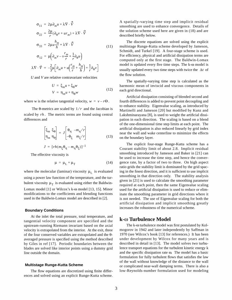
Quasi-3-D Navier-Stokes EquationsThe Navier-Stokes equations have been developed in

an coordinate system as shown in figure 1. Herem is the arc length along the surface,

(1)

and the θ-coordinate is fixed to the blade row and rotateswith angular velocity Θ.

The radius r and the thickness h of the stream surfaceare assumed to be known functions of m. The equationshave been mapped to a body-fitted coordinate system, sim-plified using the thin layer approximation, and nondimen-sionalized by arbitrary reference quantities , , and

. The Reynolds number Re and Prandtl number Pr are

defined in terms of these reference quantities. The finalequations are given in [14] and are summarized below.

(2)

where

(3)

(4)

(5)

(6)

is the total energy per unit volume,

(7)

is the pressure,

, and (8)

are derivatives of the streamtube geometry, and

(9)

The viscous fluxes are given by

(10)

is the speed of sound squared. Using Stokes’

hypothesis, , the shear stress terms are given by

m θ,( )

Figure 1. Quasi-three-dimensional stream surface for acompressor rotor.

θ

z

h(m)

r(m)

m

dm2

dz2

dr2

+=

ρ0 c0

µ0

∂tq ∂ξE ∂η F Re1–S–( )+ + K=

q J 1– ρ ρu ρvr e, , ,T=

J 1– 0 K2 0 0, , ,T

=

S J 1– 0 S2 S3 S4, , ,T

=

E J1–

ρU

ρuU ξm p+

ρvU ξθ p+( )r

e p+( )U ξθrΩp+

=

F J1–

ρV

ρuV ηm p+

ρvV ηθ p+( )r

e p+( )V ηθrΩp+

=

e ρ CvT12--- u2 v2+( )+=

p γ 1–( ) e12--- u2 v2+( )–=

rm

r------

1r---

mddr

=hm

h------

1h---

mddh

=

K2 ρv2 p Re1– σ22–+( )

rm

r------ p Re

1– σ33–( )hm

h------+=

S2 ηmσ11 ηθσ12+=

S3 ηmσ12 ηθσ22+( )r=

S4µ

γ 1–( )Pr---------------------- ηm

2 ηθ2+( )∂ηa2 uS2 vS3+ +=

a2 γ p ρ⁄=

λ 23---µ–=

3

(11)

U and V are relative contravariant velocities

(12)

where w is the relative tangential velocity, .

The θ-metrics are scaled by and the Jacobian is

scaled by . The metric terms are found using centraldifferences and

(13)

The effective viscosity is

(14)

where the molecular (laminar) viscosity is evaluated

using a power law function of the temperature, and the tur-bulent viscosity is evaluated using either the Baldwin-

Lomax model [1] or Wilcox’s k-ω model [13, 15]. Minormodifications to the coefficients and blending functionsused in the Baldwin-Lomax model are described in [2].

Boundary Conditions

At the inlet the total pressure, total temperature, andtangential velocity component are specified and theupstream-running Riemann invariant based on the axialvelocity is extrapolated from the interior. At the exit, threeof the four conserved variables are extrapolated and the θ-averaged pressure is specified using the method describedby Giles in ref [17]. Periodic boundaries between theblades are solved like interior points using a dummy gridline outside the domain.

Multistage Runge-Kutta Scheme

The flow equations are discretized using finite differ-ences and solved using an explicit Runge-Kutta scheme.

A spatially-varying time step and implicit residualsmoothing are used to enhance convergence. Details ofthe solution scheme used here are given in (18) and aredescribed briefly below.

The discrete equations are solved using the explicitmultistage Runge-Kutta scheme developed by Jameson,Schmidt, and Turkel [19]. A four-stage scheme is used.For efficiency, physical and artificial dissipation terms arecomputed only at the first stage. The Baldwin-Lomaxmodel is updated every five time steps. The k-ω model isusually updated every two time steps with twice the ofthe flow solution.

The spatially-varying time step is calculated as theharmonic mean of inviscid and viscous components ineach grid directional.

Artificial dissipation consisting of blended second andfourth differences is added to prevent point decoupling andto enhance stability. Eigenvalue scaling, as introduced byMartinelli and Jameson [20] but modified by Kunz andLakshminarayana [8], is used to weight the artificial dissi-pation in each direction. The scaling is based on a blendof the one-dimensional time step limits at each point. Theartificial dissipation is also reduced linearly by grid indexnear the wall and wake centerline to minimize the effectson the boundary layer.

The explicit four-stage Runge-Kutta scheme has aCourant stability limit of about 2.8. Implicit residualsmoothing introduced by Jameson and Baker in [21] canbe used to increase the time step, and hence the conver-gence rate, by a factor of two to three. On high aspectratio grids the stability limit is dominated by the grid spac-ing in the finest direction, and it is sufficient to use implicitsmoothing in that direction only. The stability analysisgiven in [21] is used to calculate the smoothing parameterrequired at each point, then the same Eigenvalue scalingused for the artificial dissipation is used to reduce or elim-inate the smoothing parameter in grid directions where itis not needed. The use of Eigenvalue scaling for both theartificial dissipation and implicit smoothing greatlyincreases the robustness of the numerical scheme.

k-ω Turbulence ModelThe k-ω turbulence model was first postulated by Kol-

mogorov in 1942 and later independently by Saffman in1970 (see Wilcox’s book [13] for references.) It has beenunder development by Wilcox for many years and isdescribed in detail in [13]. The model solves two turbu-lence transport equations for the turbulent kinetic energy kand the specific dissipation rate ω. The model has a basicformulation for fully turbulent flows that satisfies the lawof the wall without knowledge of the distance to the wallor complicated near-wall damping terms. There is also alow-Reynolds-number formulation used for modeling

σ11 2µ∂mu λ∇ V⋅+=

σ222µr

------ ∂θv urm+( ) λ∇ V⋅+=

σ33 2µuhm

h------ λ∇ V⋅+=

σ12 µ ∂mv vrm

r------–

1r---∂θu+

=

λ∇ V⋅ 23---µ ∂mu u

rm

r------

hm

h------+

1r---∂θv+ +–=

U ξmu ξθw+=

V ηmu ηθw+=

w v rΘ–=

1 r⁄rh

ξm ξθ

ηm ηθJ

θη mη r⁄–

θξ– mξ r⁄=

J rh mξθη mηθξ–( )[ ] 1–=

µ µL µT+=

µL

µT

∆t

4

transition [15]. Boundary conditions can be specified tosimulate mass injection or surface roughness.

Most of Wilcox’s development of the model usedboundary layer codes, but recently Menter has shown sev-eral applications to Navier-Stokes codes [16]. Menterfound that the model exhibited strong dependence onfreestream values of ω and proposed a somewhat ad hocfix. In this work many of Menter’s suggestions for numer-ical implementation of the model have been used, but hisfix for the problem of freestream dependence has not.

The quasi-3-D form of the k-equation has beenderived by writing the m- and θ-momentum equations innon-conservative form, multiplying each by its fluctuatingvelocity component, and Favre averaging. The usual tur-bulence modeling approximations are made, i. e., theBoussinesq model is used for the Reynolds stress terms,pressure work, diffusion, and dilatation are all neglected,and turbulent dissipation is taken to be proportional to

. The production term is written in terms of the vor-ticity magnitude using Menter’s suggestion [16]. Sourceterms that arise from the quasi-3-D equations areneglected. The ω-equation is derived from the k-equationby dimensional considerations. Wilcox’s constants areused without modification. The final form of the modelequations is as follows:

(15)

where

(16)

(17)

The molecular plus turbulent diffusion terms G arewritten using the thin-layer approximation giving

(18)

Menter’s form of the production terms is used [16].

(19)

where

(20)

is the vorticity. The destruction terms are given by

(21)

The baseline k-ω model has five coefficients:

, , , , ,

and the trivial constant .

The low-Reynolds-number model replaces three ofthe constants with the following bilinear functions of theturbulence Reynolds number :

, , and ,

where

(22)

with , ,

and , , .

Boundary Conditions

At the inlet the turbulence intensity Tu and turbulentviscosity are specified. Then k and ω are found from

(23)

where for the baseline model or for the

low-Reynolds-number model. Substituting equation (22)

for into equation (17) for gives a quadratic for

. The solution is

(24)

and ω may be found from

k ω×

∂tq U∂ξq V ∂ηq Re 1– Jρ---G–+ +

1ρ--- P D–( )=

q k ω,T=

µT α*ρkω------=

Gηm

2 ηθ2+( )

J-------------------------

µ σ*µT+( )∂ηk

µ σµT+( )∂ηω=

Pρ---

Re 1–µT

ρ------Ω2 2

3---k ∂mu

1r---∂

θv+

–

α α*Ω2 23---ω ∂mu

1r---∂

θv+

–

=

Ω ∂mv1r---∂θu– v

rm

r------+=

Dρ---- β*ωk

βω2=

β 3 40⁄= β* 9 100⁄= σ 1 2⁄= σ* 1 2⁄= α 5 9⁄=

α* 1=

ReT

β* 9 100⁄( )Fβ= α 5 9⁄( ) Fα Fµ⁄( )= α* Fµ=

Fβ5 18⁄ ReT Rβ⁄( )4+

1 ReT Rβ⁄( )4+-----------------------------------------------=

Fαα0 ReT Rω⁄+

1 ReT Rω⁄+----------------------------------=

Fµα0

* ReT Rk⁄+

1 ReT Rk⁄+---------------------------------=

ReTρk

µLω-----------=

α0 1 10⁄= α0* β 3⁄ 1 40⁄= =

Rβ 8= Rω 27 10⁄= Rk 6=

µT

k32---Tu2U in

2=

ω α*ρkµT------=

α* 1= α* Fµ=

α* µT

ReT

ReT12--- α0

*Rk

µT

µL------–

– α0*Rk( )2 2Rk

µT

µL------ 2 α0

*–( )++=

5

(25)

A turbulent length scale can be defined using (17) as

(26)

The effects of varying the inlet values of ω or l is dis-cussed with the results.

On solid walls k = 0, and ω is set using Wilcox’sroughness model.

(27)

where

(28)

and is the equivalent sand grain roughness height in

turbulent wall units. For all results shown here was set

to 5, giving a hydraulically smooth surface.

To avoid numerical difficulties near leading edgeswhere becomes large, an upper limit was imposed on

ω using a boundary condition suggested by Menter [16].

(29)

where is the grid spacing at the wall.

k and ω were extrapolated at the exit and treated asperiodic across trailing edge wake cut lines and betweenblade rows.

ADI Solution Scheme

An alternating direction implicit (ADI) scheme wasused to solve the k-ω equations. An implicit scheme waschosen so that the equations could be updated less oftenthan the flow equations without stability problems, andalso because the k-ω equations are dominated by complexsource terms which are evaluated only once in an ADIscheme, but potentially at every stage of a Runge-Kuttascheme.

Equation (15) may be written as

(30)

Using first-order backward Euler time differencingand linearizing the right hand side about the previous timestep gives

(31)

where primes indicate Jacobians. The advective terms areapproximated using first-order upwind differences.

(32)

The diffusive terms (18) can be written as

(33)

Since , , and the Jacobian

is simply

(34)

The diffusive terms are approximated by second-ordercentral differences.

(35)

The difference approximations (32) and (35) are diago-nally dominant and have zero row sum, which accordingto Baldwin and Barth [22], makes the implicit operator anM-type matrix with a non-negative inverse.

Menter’s linearization is used for the source terms[16]. The production terms are treated explicitly, i.e.,

. The destruction terms are linearized using

(36)

The term in the upper right corner is the only cou-pling between the k and ω equations. Here the term hasbeen neglected and the equations are solved uncoupledfrom each other and from the flow equations.

Equation (31) is solved using an approximate factor-ization.

ω ρkµLReT----------------=

µT α*ρkω------ ρ k

α* kω

------------- ρ k l= = =

ωµτ

2

ν------SR SR y∂

∂u

wall

= =

SR

50kR

+------

2kR

+ 25<

100kR

--------- kR+ 25≥

=

kR+

kR+

µτ

ωmax10Re------ 6ν

β∆y2-------------×=

∆y

∂tq U∂ξq V ∂ηq Re 1– Jρ---∂ηG

1ρ--- P D–( )––+–=

I ∆t U∂ξ V ∂η Re 1– Jρ---∂ηG′ 1

ρ--- P′ D′–( )––++

∆q

∆t U∂ξq V ∂ηq Re 1– Jρ---∂ηG

1ρ--- P D–( )––+–=

U∂ξq U+

qi j, qi 1 j,––( ) U-

qi j, qi 1 j,+–( )–≈

U± 12--- U U±( )=

Gηm

2 ηθ2+( )

J-------------------------

µ σ*µT+( )∂ηk

µ σµT+( )∂ηω

gk∂ηk

gη∂ηω= =

σ* σ 1 2⁄= = gk gω g= =

Gv′

G′∆qq∂

∂G∆q g∂η∆k

∂η∆ω= =

∂ηg∂ηk12--- gi j, 1+ gi j,+( ) ki j, 1+ ki j,–( )

gi j, 1– gi j,+( ) ki j, 1– ki j,–( )+

[

]

≈

P′ 0=

D′ρ------ β*ω β*k

0 2βω=

β*k

6

(37)

The destruction terms are included with the

streamwise operator. Treating the destruction termsimplicitly improves the diagonal dominance but gives theimplicit operator a nonzero row sum.

The Baldwin-Lomax and k-ω models have both beencoded fairly efficiently. A turbulent flow solution updatingthe Baldwin-Lomax every time step model takes 1.53times as long as a laminar solution. Past experience hasshown that it is sufficient to update the Baldwin-Lomaxmodel every five time steps, reducing the CPU time toabout 1.1 times that of a laminar solution. A solutionupdating the k-ω equations takes 1.6 times as long as alaminar solution. Some cases have been successfully com-puted updating the k-ω equations every five time steps(with five times the of the flow solution), making the k-ω model nearly as fast as the Baldwin-Lomax model.Other cases failed to converge unless the k-ω equationswere updated every other time step, and that strategy hasbeen used for all results reported here. The net result isthat a flow solution with the k-ω model takes about 1.18times as long as a solution with the Baldwin-Lomaxmodel.

I ∆t U∂ξD′ρ------+

+ I ∆t V ∂η Re 1– Jρ---∂ηGv′–

+ ∆q

∆t U∂ξq V ∂ηq Re 1– Jρ---Gv

1ρ--- P D–( )––+–=

D′ξ

∆t

Results

Flat Plate Boundary Layer

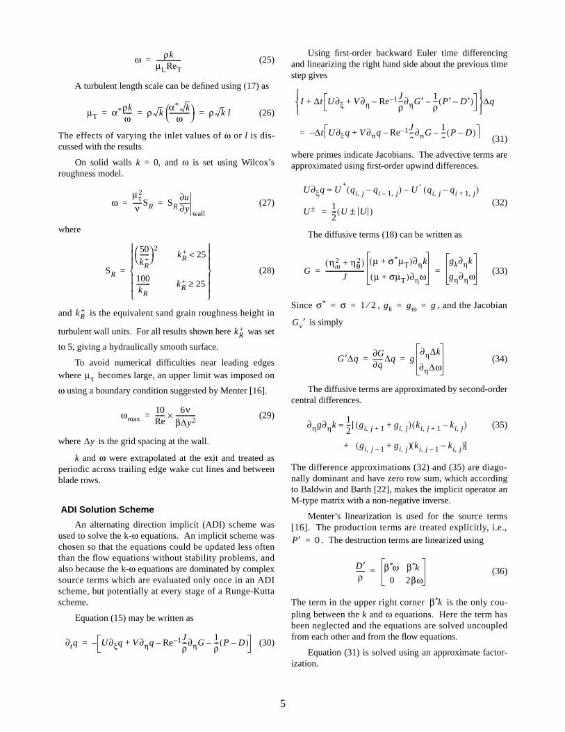
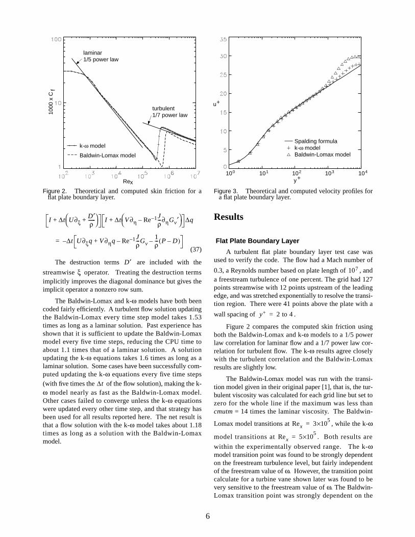
A turbulent flat plate boundary layer test case wasused to verify the code. The flow had a Mach number of

0.3, a Reynolds number based on plate length of , anda freestream turbulence of one percent. The grid had 127points streamwise with 12 points upstream of the leadingedge, and was stretched exponentially to resolve the transi-tion region. There were 41 points above the plate with a

wall spacing of .

Figure 2 compares the computed skin friction usingboth the Baldwin-Lomax and k-ω models to a 1/5 powerlaw correlation for laminar flow and a 1/7 power law cor-relation for turbulent flow. The k-ω results agree closelywith the turbulent correlation and the Baldwin-Lomaxresults are slightly low.

The Baldwin-Lomax model was run with the transi-tion model given in their original paper [1], that is, the tur-bulent viscosity was calculated for each grid line but set tozero for the whole line if the maximum was less thancmutm = 14 times the laminar viscosity. The Baldwin-

Lomax model transitions at , while the k-ω

model transitions at . Both results are

within the experimentally observed range. The k-ωmodel transition point was found to be strongly dependenton the freestream turbulence level, but fairly independentof the freestream value of ω. However, the transition pointcalculate for a turbine vane shown later was found to bevery sensitive to the freestream value of ω. The Baldwin-Lomax transition point was strongly dependent on the

107

y+ 2 to 4=

Rex 35×10=

Rex 55×10=

Rex

1000

x C

flaminar1/5 power law

turbulent1/7 power law

Baldwin-Lomax model

k-ω model

100 101 102 103 104

y+

u+

Spalding formulak-ω modelBaldwin-Lomax model

Figure 2. Theoretical and computed skin friction for aflat plate boundary layer.

Figure 3. Theoretical and computed velocity profiles fora flat plate boundary layer.

7

0.70

0.90

1.30

1.40

0.70

0.80

0.80

0.80

0.80

0.80

0.80

0.90

0.90

0.90

1.001.00

1.30

1.40

1.4

0

1.4

0

1.40

1.4

0

1.30

1.40

1.40

1.5

01.5

0

1.00

1.00

1.3

0

1.4

01.4

0

1.40

0.70

0.80

0.80

0.80

0.60

0.90

1.4

01.4

0

1.5

0

1.3

0

0.70

0.80

0.80

0.60

0.90

1.5

0

computedBaldwin-Lomax / k-ω measured

Baldwin-Lomax model k-ω model

Figure 4. Computed and measured contours of relative Mach number for a transonic compressorrotor.

Figure 5. Turbulent viscosity contours around a transonic compressor rotor.

8

0 40 80 120 160 200 percent pitch

1.0

0.8

0.6

0.4

0.2

Mre

l

experimental datak-ω modelBaldwin-Lomax model

0 40 80 120 160 200 percent pitch

1.2

1.0

0.8

0.6

0.4

Mre

l

experimental datak-ω modelBaldwin-Lomax model

Figure 6. Computed and measured near wake Machnumber profiles for a transonic compressor rotor.

Figure 7. Computed and measured far wake Machnumber profiles for a transonic compressor rotor.

value of the cutoff parameter cmutm, suggesting that thisparameter could be calibrated to simulate freestream tur-bulence effects.

Figure 3 compares computed velocity profiles locatedat the end of the plate to Spalding’s composite sublayer/law-of-the-wall profile. Both results agree closely, but theBaldwin-Lomax profile has a slightly stronger wake com-ponent.

Transonic Compressor Rotor

The transonic compressor rotor described by Suder etal. [3] was used to test the quasi-3-D effects in the model.

The rotor was tested experimentally at NASA LewisResearch Center using both laser anemometry and conven-tional aero probes.

A section of the rotor at 70 percent span was ana-lyzed. The radius was specified as a line 70 percent of theway between the hub and shroud, and the stream surfacethickness was specified as the local distance between thehub and shroud, normalized to one at the inlet. A meridi-onal view of the streamtube is shown in figure 1. A C-typegrid was used with 319 points around the blade and 45

points away from the blade. The grid spacing gaveover most of the blade. The calculations were run 2000iterations, which took about 3.25 minutes for the k-ωmodel on the Cray C-90 called eagle at NASA AmesResearch Center.

Figure 4 compares contours of relative Mach numbercomputed with the k-ω model (the Baldwin-Lomax modelgives identical contours) to contours measured experimen-tally using laser anemometry. The inlet Mach number is

about 1.4. The flow passes through a weak upstream-run-ning wave system, then through a strong normal passageshock, and leaves the rotor at about Mach 0.8. The com-puted Mach number behind the normal shock is somewhatlower than the measured values. This is partly due to theassumed stream surface but may also be partly due to theinability of either turbulence model to capture the shock-boundary layer interaction correctly.

One motivation for using a turbulent transport modelwas that algebraic models frequently fail to find the correctlength scale and thus give nonsmooth values of [2].

Occasionally nonconvergence or instability problems canbe traced to poor numerical behavior of the turbulencemodel. Figure 5 shows contours of computed using

the Baldwin-Lomax model (left) and the k-ω model(right.)

Figure 4 also shows that the computed results seri-ously underpredict the wake spreading. This is shownquantitatively in figures 6 and 7. Figure 6 compares com-puted and measured near-wake profiles about 0.28 chordsdownstream of the trailing edge while figure 7 comparesfar-wake profiles about 2 chords downstream. The twoturbulence models give surprisingly similar results, espe-cially considering the erratic behavior of the Baldwin-Lomax model seen in figure 5.

The computed wakes are both narrower and deeperthan the measured wakes. Wilcox has shown in [13] thathis model gives the best prediction for planar wake spread-ing as . This limit corresponds to ,

which seems unreasonable for an inlet value. Varying

by five orders of magnitude had very little effect on the

y+ 2<

µT

µT

ωin 0→ µT ∞→

ωin

9

computed wake spreading. The freestream turbulence wasset to three percent, and doubling it had little effect on thewake spreading.

Transonic Turbine Cascade

A transonic turbine vane tested by Arts, et al. [23] wascomputed as a third test case. The vane was tested experi-mentally in the Isentropic Light Piston Compression TubeFacility at the von Karman Institute. The facility has inde-pendent control over the exit Reynolds number , the

exit Mach number, , and the inlet turbulence inten-

sity Tu. Surface pressures were measured with static taps,and wake total pressure profiles were measured with ahigh-speed traversing probe. The vanes were initially at300 K and the freestream temperature was 415 K.Unsteady blade surface temperatures were measured dur-ing a run using platinum thin film gauges, then convertedto heat fluxes using a one-dimensional semi-infinite-bodymodel.

For the computations a C-type grid was used with 383points around the vane and 49 points away from the vane.

The grid spacing gave over most of the vane.Blade shapes and computed Mach contours for

are shown in figure 8. The flow accelerates

Re2,is

M2,is

y+ 1.5<

2,is 0.9=

from a Mach number of about 0.15 at the inlet to about 0.9at the exit.

Surface heat transfer was converged to plotting accu-racy in 3000 iterations in fully turbulent regions. Laminarparts of the flow took longer to converge, so all calcula-tions were run 5000 iterations. Solution times were abouteight minutes per case on the Cray C-90 computer. A typi-cal residual history is shown in figure 9. The k-ω calcula-tions converged monotonically, but with the Baldwin-Lomax model the maximum residual oscillated near theround trailing edge.

Computed distributions of isentropic surface Machnumber are compared to experimental data for =

0.875 and 1.02 in figure 10. The Baldwin-Lomax and k-ωmodels give identical results and are not shown separately.The subsonic results agree very well with the experimentaldata. The transonic results slightly underpredict the Machnumber on the rear (uncovered) part of the suction surface.All subsequent results are for the subsonic case.

Computed wake profiles located 43 percent of axialchord downstream of the trailing edge are compared to theexperimental data (digitized manually from [23]) in figure11. Again the computed wakes are narrower and deeperthan the measured wakes, but here the k-ω results areslightly better than the Baldwin-Lomax results.

Figures 12 - 15 show the effects of various parameters

on surface heat transfer coefficient H . In

each figure the abscissa is the arc length S [mm] along thevane surface. Figure 12 compares computations using thebaseline k-ω model, the low-Reynolds-number k-ω model,and the Baldwin Lomax model to experimental data for

2,is

W/(m2K )[ ]

.9

.8

.3.2

.9

1.

.9

.8

.9

.8

.3.2

.9

1.

.9

.8

.9

Figure 8. Computed Mach number contours for the VKIturbine vane.

Iterations

resi

dual

max.

rms

Baldwin-Lomax

k-ω

Baldwin-Lomax

k-ω

Figure 9. Residual histories for the VKI turbine vanecomputations.

10

0 20 40 60 80 100

Mis

en

2,isM expt. comp.1.020.875

S (mm)

H (

W /

m

K)

2

pressure surface suction surface

baseline k-ωlow Re k-ωBaldwin-Lomaxexpt., Tu = 4%

S (mm)

H (

W /

m

K)

2

pressure surface suction surface

expt. comp.

641

T (%)u

S (mm)

H (

W /

m

K)

2

pressure surface suction surface

l (mm) comp. in7.25e-27.25e-42.50e-46.25e-5

µ /µT,in ref 1.0e 11.0e-13.5e-29.0e-3

S (mm)

H (

W /

m

K)

2

pressure surface suction surface

Re expt. comp.2,is2. M1. M.5 M

1-P

/P

02

01

experimental dataBaldwin-Lomax modelk-ω model

Figure 10. Computed and measured distributions ofisentropic Mach number for the VKI turbine vane.

Figure 11. Computed and measured total pressure profiles0.43 chords behind the VKI turbine vane.

Figure 12. Surface heat transfer coefficient predicted bythree turbulence models.

Figure 13. Effects of inlet turbulent length scale orviscosity on predicted heat transfer coefficient.

Figure 15. Effects of Reynolds number on heat transfercoefficient

Figure 14. Effects of inlet turbulence intensity on heattransfer coefficient.

11

and Tu = 4 percent. Triangles show the

experimental data. The baseline k-ω solution is fully tur-bulent on the suction surface giving high values of H. Thepressure surface has a highly favorable pressure gradientand acts laminar over part of the chord, transitioning nearS = -20. The low-Reynolds-number k-ω solution remainslaminar on the pressure surface and transitions near themeasured transition point on the suction surface; however,the transition point was forced by choice of , as dis-

cussed later. The Baldwin-Lomax solution agrees closelywith the low-Reynolds-number k-ω solution. As dis-cussed with figure 14, the laminar parts of the flow haveaugmented heat transfer due to freestream turbulence thatnone of the models predict.

Figure 13 shows the effects of or the corre-

sponding length scale on H for the same flow condi-

tions. The inlet turbulent viscosity was varied by about 3orders of magnitude to produce solutions that ranged fromfully laminar to almost fully turbulent. Only a small rangeof values of gave transition near the measured loca-

tion. Corresponding turbulence length scales are shownon the figure. The length scale that gives the best transi-

tion location, , is about 1/1600 times the

pitch or about 7 times the grid spacing at the wall. Allsubsequent calculations were run with this length scale.Although this strong dependence on is disconcerting

since appropriate values are not known in advance, Wilcoxpoints out that transition in real flows is not simply a func-tion of Tu, but is also frequency dependent [15]. He alsosuggests that two coefficients in the low-Reynolds-numbermodel could be adjusted to better match other flows,although this has not been attempted here.

The effects of freestream turbulence intensity Tu areshown in figure 14. The effect on suction surface transi-tion location is modeled reasonably well by the low-Rey-nolds-number k-ω model. The experimental data shows astrong augmentation of heat transfer at the leading edgeand on the pressure surface as Tu is increased. Althoughthe low-Reynolds-number k-ω model depends directly onTu, in laminar regions the model gives values of turbulentviscosity that are much too small to affect the heat transfer.Boyle has added algebraic correlations to the Baldwin-Lomax model to simulate freestream turbulence effects[4]. These correlations could be added to the k-ω code,but they do involve the distance from the wall.

The effects of Reynolds number are shown in

figure 15 for Tu = 4 percent. The data shows a largeincrease in heat transfer with . The k-ω results show

qualitative agreement, but the magnitude of the heat trans-fer is underpredicted due to the failure of the model to pre-

dict freestream turbulence effects. Effects on suctionsurface transition location are overpredicted, and predictedtransition is too abrupt. The data shows transition on thepressure surface at the highest Reynolds number that is notpredicted, although a small change in does cause

pressure surface transition, as shown in figure 13.

Concluding RemarksWilcox’s k-ω turbulence model has been added to a

quasi-3-D Navier-Stokes analysis code for turbomachin-ery. The code includes the effects of rotation, radiuschange, and stream sheet convergence, and also includedthe Baldwin-Lomax turbulence model. The quasi-3-Dflow equations and boundary conditions were described.An explicit multistage Runge-Kutta scheme with spatially-varying time step and implicit residual smoothing wasused to solve the flow equations. The quasi-3-D form ofthe k-ω model equations and boundary conditions werealso described. An upwind implicit ADI scheme was usedto update the turbulence model equations uncoupled fromthe flow equations. The numerical scheme was quiterobust, but about 18 percent slower than the Baldwin-Lomax model.

Calculations were made for three test cases: a flatplate boundary layer with transition, a transonic compres-sor rotor with significant quasi-3-D effects, and a transonicturbine vane. The flat plate calculations agreed very wellwith theory for both turbulence models. Transition predic-tions were reasonable for both models and suggested thatthe Baldwin-Lomax transition model could be calibratedto simulate free stream turbulence effects. The compres-sor rotor calculations showed very close agreementbetween the two turbulence models, but both models failedto capture the measured wake spreading. The turbine cal-culations showed very good agreement with measured sur-face pressures for both turbulence models. Predicted wakeprofiles were thinner and deeper than measured profiles,although the k-ω model gave marginally better results.The Baldwin-Lomax model, the baseline k-ω model, andthe low-Reynolds-number k-ω model were compared forheat transfer calculations. The Baldwin-Lomax model didreasonably well considering the simple transition modelused. The low-Reynolds-number k-ω model showed ahigh sensitivity to inlet values of ω, expressed as an inletturbulent viscosity or length scale which are not generallyknown. The k-ω model was able to capture the effects ofinlet turbulence intensity on transition but not on augmen-tation of heat transfer in laminar regions. It may be possi-ble to model this effect with a simple algebraic model.Effects of Reynolds number were predicted qualitatively.

The k-ω model exhibited some attractive numericalproperties, but for the cases considered here, predictionswere not decisively better than those made with the Bald-win-Lomax model. Other test cases may identify areas

Re2 is, 16×10=

µT,in

µT,in

lin

µT,in

lin 3.52–×10=

µT,in

e2,is

e2,is

µT,in

12

where the k-ω model is significantly better than the Bald-win-Lomax model. Future work will extend the k-ωmodel to three dimensions where algebraic models arepoorly defined and difficult to implement.

References

1. Baldwin, B. S., and Lomax, H., “Thin-LayerApproximation and Algebraic Model for SeparatedTurbulent Flows,” AIAA Paper 78-257, Jan. 1978.

2. Chima, R. V., Giel, P. W., and Boyle, R. J., “AnAlgebraic Turbulence Model for Three-Dimen-sional Viscous Flows,” NASA TM-105931, Jan.1993.

3. Suder, K. L., Chima, R. V., Strazisar, A., J., andRoberts, W., B., ‘‘The Effect of Adding Thicknessand Roughness to a Transonic Axial CompressorRotor,’’ ASME Paper 94-GT-339, June 1994.

4. Boyle, R. J., ‘‘Navier-Stokes Analysis of TurbineBlade Heat Transfer,’’ ASME Paper 90-GT-42, June1990 (also NASA TM 102496).

5. Menter, F., R., ‘‘Performance of Popular Turbu-lence Models for Attached and Separated AdversePressure Gradient Flows,’’ AIAA Journal, Vol. 30,No. 8, Aug. 1992, pp. 2066-2071.

6. Choi, D., and Knight, C. J., “Computations of 3DViscous Flows in Rotating TurbomachineryBlades,” AIAA Paper 89-0323, Jan. 1989.

7. Hah, C., and Wennerstrom, A. J., “Three-Dimen-sional Flowfields Inside a Transonic CompressorWith Swept Blades,” ASME Paper 90-GT-359, June1990.

8. Kunz, R. F., and Lakshminarayana, B., “Computa-tion of Supersonic and Low Subsonic CascadeFlows Using an Explicit Navier-Stokes Techniqueand the k-ε Turbulence Model,” in ComputationalFluid Dynamics Symposium on Aeropropulsion,NASA CP-10045, Apr. 1990.

9. Ameri, A., and Arnone, A., “Navier-Stokes TurbineHeat Transfer Predictions Using Two-Equation Tur-bulence Closure,” AIAA Paper 92-3067, July 1992(also NASA TM-105817).

10. Ameri, A., and Arnone, A., “Prediction of TurbineBlade Passage Heat Transfer Using a Zero and aTwo-Equation Turbulence Model,” ASME Paper94-GT-122, June 1994.

11. Basi, F., Rebay, S., and Savini, M., “A Navier-Stokes Solver with Different Turbulence ModelsApplied to Film-Cooled Turbine Cascades,” in HeatTransfer and Cooling in Gas Turbines, AGARD-CP-527, Oct. 1992, pp. 41.1 to 41.16.

12. Liu, F., and Zheng, X., “Staggered Finite VolumeScheme for Solving Cascade Flow with a k-ω Tur-bulence Model,” AIAA Journal, Vol. 32, No. 8, Aug.1994, pp. 1589-1597.

13. Wilcox, D., C., Turbulence Modeling for CFD,DCW Industries, Inc., La Canada, CA, 1994.

14. Chima, Rodrick V., “Explicit Multigrid Algorithmfor Quasi-Three-Dimensional Viscous Flows inTurbomachinery,” AIAA Journal of Propulsion andPower, Vol. 3, No. 5, Sept.-Oct. 1987, pp. 397-405.

15. Wilcox, D., C., ‘‘Simulation of Transition with aTwo-Equation Turbulence Model,’’ AIAA Journal,Vol. 32, No. 2, Feb. 1994, pp. 247-255.

16. Menter, F., R., ‘‘Improved Two-Equation k-ω Tur-bulence Model for Aerodynamic Flows,’’ NASATM-103975, Oct. 1992.

17. Giles, M. B., “Nonreflecting Boundary Conditionsfor Euler Equation Calculations,” AIAA Journal,Vol. 28, No. 12, Dec. 1990, pp. 2050-2058.

18. Tweedt, D. L., and Chima, R. V., ‘‘Rapid NumericalSimulation of Viscous Axisymmetric Flow Fields,’’submitted for presentation at AIAA 34th AerospaceSciences Meeting, Jan. 15-18, 1996.

19. Jameson, A., Schmidt, W., and Turkel, E., “Numer-ical Solutions of the Euler Equations by Finite Vol-ume Methods Using Runge-Kutta Time-SteppingSchemes,” AIAA Paper 81-1259, June 1981.

20. Martinelli, L., and Jameson, A., “Validation of aMultigrid Method for the Reynolds Averaged Equa-tions,” AIAA Paper 88-0414, Jan. 1988.

21. Jameson, A., and Baker, T. J., “Solution of theEuler Equations for Complex Configurations,”AIAA Paper 83-1929, July 1983.

22. Baldwin, B. S., and Barth, T. J., ‘‘A One-EquationTurbulence Transport Model for High ReynoldsNumber Wall-Bounded Flows,’’ NASA TM102847, Aug. 1990.

23. Arts, T., Lambert de Rouvroit, M., and Rutherford,A., W., ‘‘Aero-Thermal Investigation of a HighlyLoaded Transonic Linear Turbine Guide Vane Cas-cade,’’ von Karman Institute Technical Note 174,Sep. 1990.